





1. Introduction
One of the key obstacles to the development of hypersonic vehicles has been the prediction and control of the laminar–turbulent boundary-layer transition. The performance of hypersonic vehicles may be compromised by the transition, as it would escalate skin friction and heat flux (Fedorov Reference Fedorov2011). Therefore, accurate transition prediction and effective control (or delay) technologies are crucial for the design of hypersonic vehicles, particularly regarding the thermal protection system. Transition induced by free-stream disturbances with low amplitudes usually follows four stages: receptivity (excitation of initial disturbance inside the boundary layer), linear instability (including modal and non-modal growth), nonlinear instability and parametric resonance and breakdown to turbulence (Morkovin et al. Reference Morkovin1994). Hypersonic boundary-layer transition over two-dimensional or axisymmetric models at a zero angle of attack is typically triggered by the growth of unstable modes, known as the first mode, associated with the vorticity disturbance (Smith Reference Smith1989), and the Mack second mode of acoustic nature (Mack Reference Mack1975; Fedorov Reference Fedorov2003; Ma & Zhong Reference Ma and Zhong2003; Chen, Guo & Wen Reference Chen, Guo and Wen2023a ). In realistic flight or wind tunnel conditions, these two types of instabilities tend to coexist and compete with one another.
Regarding the breakdown or parametric resonance, several scenarios have been confirmed by numerous direct numerical simulations (DNS) and experimental studies. These include the first-mode-dominated subharmonic resonance (Kosinov et al. Reference Kosinov, Semionov, Shevel’kov and Zinin1994), the first-mode-dominated oblique breakdown (Mayer, Von Terzi & Fasel Reference Mayer, Von Terzi and Fasel2011), the second-mode oblique breakdown (Hartman, Hader & Fasel Reference Hartman, Hader and Fasel2021), the second-mode-dominated fundamental resonance (Hader & Fasel Reference Hader and Fasel2019; Kennedy et al. Reference Kennedy, Jewell, Paredes and Laurence2022; Unnikrishnan & Gaitonde Reference Unnikrishnan and Gaitonde2020) and the second-mode subharmonic resonance (Bountin, Shiplyuk & Maslov Reference Bountin, Shiplyuk and Maslov2008; Franko & Lele Reference Franko and Lele2013). These conventional transition scenarios are characterised by tuned modes with frequencies that are integer times $f_{1/2}$
; here,
$f_{1/2}$
; here, $f_{1/2}$
refers to half of the frequency of the primary instability wave. The dominating transition scenario depends on the specific numerical forcing with given flow and geometric conditions. In a realistic disturbance environment, several primary instabilities can be excited simultaneously and coexist. In this case, complex mode–mode interactions emerge, and detuned modes may be pronounced (Fezer & Kloker Reference Fezer and Kloker2000). As reported by Chen et al. (Reference Chen, Zhu and Lee2017) for the flared-cone model at Peking University, multiple primary instabilities give rise to complex nonlinear interactions and significant energy transfer between low- and high-frequency components. A possible combination resonance is also indicated, which differs from that induced by a single primary instability (Franko & Lele Reference Franko and Lele2013; Hader & Fasel Reference Hader and Fasel2019). Nonetheless, direct evidence in the transitional stage was not provided. Recently, Guo et al. (Reference Guo, Hao and Wen2023a
) have demonstrated the significance of the non-conventional combination resonance associated with modal detuning in the high-speed boundary-layer transition. The nonlinear interaction between low-frequency first mode and high-frequency second mode can produce a new breakdown scenario. This multiple-primary-instabilities scenario is believed to be noteworthy, since multiple instabilities are seeded in realistic boundary layers. As an extension, the effect of flow control on the breakdown scenario is of particular interest.
$f_{1/2}$
refers to half of the frequency of the primary instability wave. The dominating transition scenario depends on the specific numerical forcing with given flow and geometric conditions. In a realistic disturbance environment, several primary instabilities can be excited simultaneously and coexist. In this case, complex mode–mode interactions emerge, and detuned modes may be pronounced (Fezer & Kloker Reference Fezer and Kloker2000). As reported by Chen et al. (Reference Chen, Zhu and Lee2017) for the flared-cone model at Peking University, multiple primary instabilities give rise to complex nonlinear interactions and significant energy transfer between low- and high-frequency components. A possible combination resonance is also indicated, which differs from that induced by a single primary instability (Franko & Lele Reference Franko and Lele2013; Hader & Fasel Reference Hader and Fasel2019). Nonetheless, direct evidence in the transitional stage was not provided. Recently, Guo et al. (Reference Guo, Hao and Wen2023a
) have demonstrated the significance of the non-conventional combination resonance associated with modal detuning in the high-speed boundary-layer transition. The nonlinear interaction between low-frequency first mode and high-frequency second mode can produce a new breakdown scenario. This multiple-primary-instabilities scenario is believed to be noteworthy, since multiple instabilities are seeded in realistic boundary layers. As an extension, the effect of flow control on the breakdown scenario is of particular interest.
Boundary-layer transition control strategies are useful in delaying the occurrence of transition. These strategies can be categorised into active methods, such as wall cooling and heating (Zhao et al. Reference Zhao, Wen, Tian, Long and Yuan2018b ; Zhou et al. Reference Zhou, Liu, Lu, Kang and Yan2022), and passive methods, such as the acoustic metasurface implemented by a porous coating (Fedorov et al. Reference Fedorov, Malmuth and Rasheed2001; Zhao et al. Reference Zhou, Liu, Lu, Kang and Yan2022). The acoustic metasurface, including the absorptive acoustic metasurface, the impedance-near-zero acoustic metasurface and the reflection-controlled acoustic metasurface, was proposed mainly to suppress the second mode of acoustic nature (Zhao et al. Reference Zhou, Liu, Lu, Kang and Yan2022). The passive approach is flexible for implementation and requires no additional energy input, which has attracted growing interest from both academia and industry. Experimental observations have shown that the porous coating can successfully postpone the transition onset (Rasheed, Hornung & Fedorov Reference Rasheed, Hornung, Fedorov and Malmuth2002; Fedorov et al. Reference Fedorov2003; Wagner et al. Reference Wagner, Kuhn, Martinez Schramm and Hannemann2013, Reference Wagner, Hannemann and Kuhn2014). However, a porous coating leads to an undesirable increment of wall friction and flux during the late stage of transitional flow. This phenomenon has been observed experimentally (Wartemann, Wagner & Kuhn Reference Wartemann, Wagner, Kuhn, Eggers and Hannemann2015) but remains poorly understood.
In the linear stability stage, the effect of the porous coating can be theoretically described and satisfactorily predicted using linear stability theory (LST) with the deduced acoustic impedance boundary condition (Fedorov et al. Reference Fedorov, Malmuth and Rasheed2001). The physical mechanism by which the porous coating influences the linear stage has been widely studied (Fedorov et al. Reference Fedorov2003; Tian & Wen Reference Tian and Wen2021; Chen et al. Reference Chen, Guo and Wen2023b ; Ji, Dong & Zhao Reference Ji, Dong and Zhao2023). It is known that viscous effects within the pores of the porous coating can dissipate the second-mode instability. Acoustic wave reflection is also linked to regimes with phase cancellation or reinforcement (Bres et al. Reference Brès, Inkman and Colonius2013). The porous coating effect in the nonlinear regime has also been the subject of early research (Tullio et al. Reference De Tullio and Sandham2010; Hader et al. Reference Hader, Brehm and Fasel2013, Reference Hader, Brehm and Fasel2014). Tullio et al. (Reference De Tullio and Sandham2010) conducted the first DNS of nonlinear breakdown with directly resolved pore-scale flow in an acoustic metasurface. Their study provided a detailed analysis of how porous coatings affect secondary instabilities for both first and second instability modes individually. Hader et al. (Reference Hader, Brehm and Fasel2013, Reference Hader, Brehm and Fasel2014) discovered that the second-mode fundamental breakdown caused a delayed transition onset. However, these investigations are restricted to single-primary-mode perturbations and the resulting typical breakdown situations, which may not accurately represent the transitional flow with broadband disturbances in wind tunnels or flight tests. Recently, Sousa et al. (Reference Sousa, Wartemann and Wagner2024) investigated the hypersonic transition delay over a broadband wall impedance using dynamic large-eddy simulation. Good agreement was observed with experimental data in the literature. The corresponding wind tunnel experiment features a high-enthalpy flow with a highly cooled wall condition, where the first mode is significantly suppressed. Consequently, the nonlinear interaction between the low-frequency first mode and the high-frequency second mode was not considered in their simulation. The resulting breakdown is more likely to be a fundamental breakdown induced by the second mode, which represents the only dominant instability under such cold-wall conditions.
Triadic interactions serve as the fundamental mechanism governing energy transfer in nonlinear flow fields, playing a well-documented role in laminar–turbulent transition. The seminal work by Craik (Reference Craik1971) established that resonant Tollmien – Schlichting wave triads can significantly accelerate transition in wall-bounded shear flows. Building on this, Rigas et al. (Reference Rigas, Sipp and Colonius2021) employed resolvent analysis incorporating nonlinear triadic interactions, demonstrating that the transition dynamics can be accurately captured using only a limited number of harmonics and their triadic couplings. To quantify such interactions, bispectral mode decomposition (BMD) proposed by Schmidt (Reference Schmidt2020) has emerged as a powerful diagnostic tool, enabling identification of dominant triads and their associated energy-transfer pathways in three-dimensional nonlinear flows. For instance, Schmidt & Oberleithner (Reference Schmidt and Oberleithner2023) applied bispectral analysis to two-phase swirling flows, revealing that triadic resonance generates a broad spectrum of secondary modes. Recent advances by Craig et al. (Reference Craig, Humble, Hofferth and Saric2019) further extended BMD to hypersonic boundary layers, where bispectral analysis of experimental data identified multiple quadratic phase-coupled sum and difference interactions. Their findings suggest that, under quiet wind tunnel conditions, the nonlinear transition mechanism is predominantly governed by high-frequency second-mode-induced fundamental breakdown. Nevertheless, this framework may not fully explain transition scenarios involving mutual interactions between low-frequency first modes and high-frequency second modes, revealing the need for further investigations on multimodal triadic coupling effects.
Even though the linear-stage stabilisation or destabilisation mechanisms are well established, how metasurfaces modulate nonlinear interactions between coexisting first and second modes – a scenario routinely encountered in practice – remains unknown. Moreover, the undesired increase of late-stage skin friction observed experimentally has yet to be explained through first-principles simulations. The current work is to examine the impact of porous coatings on the nonlinear mode–mode interaction and the resulting breakdown process. Two research objectives are included: (i) to reveal the transition delay mechanism by the acoustic metasurface subject to multiple primary instabilities; (ii) to explain why the skin friction is augmented in the late transitional stage. To this end, the effect of the metasurface is evaluated using a modelled impedance boundary condition (IBC) to avoid meshing the cavity, which can save computational costs. The time-domain impedance boundary condition (TDIBC) (Fung & Ju Reference Fung and Ju2004; Douasbin, Scalo & Selle Reference Douasbin, Scalo, Selle and Poinsot2018; Fiévet et al. Reference Fiévet, Deniau, Brazier and Piot2021; Guo, Hao & Wen Reference Guo, Liu, Zhao, Hao and Wen2023b ) can be efficiently incorporated into a Navier–Stokes solver and handle broadband disturbances. The accuracy and efficiency of TDIBC have been shown in the simulation of late transitional and turbulent boundary layers (Scalo, Bodart & Lele Reference Scalo, Bodart and Lele2015; Chen & Scalo Reference Chen and Scalo2021b ; Sousa et al. Reference Sousa, Wartemann and Wagner2024). It is anticipated that the mode–mode interaction and the resulting breakdown scenario with the acoustic metasurface will be revealed to understand why the transition onset is delayed. Moreover, regarding the enhanced skin friction in the late transition stage, which has also been observed in the experiments by Wagner et al. (Reference Wagner, Kuhn, Martinez Schramm and Hannemann2013, Reference Wagner, Hannemann and Kuhn2014), an energy budget analysis and bi-Fourier analysis are performed to explore the underlying physics.
The remainder of this paper is organised as follows. Section 2 provides an overview of the investigated model and flow parameters, the formulation of TDIBC, stability analysis tools and numerical methods for DNS. Section 3 presents the fitting results of TDIBC using a theoretical model, the results of the stability analysis and the effect of TDIBC on the linear stage. Comparative transition simulations induced by multiple disturbances with and without the acoustic metasurface are shown in §§ 4 and 5. The instantaneous and time-averaged flow fields, bi-Fourier analysis, results of BMD and energy budget analysis are included. Section 4 characterises the three-dimensional flow structure and provides statistical analysis of mean-flow properties, while § 5 investigates the nonlinear mode – mode interactions and subsequent breakdown dynamics. The principal findings and their physical implications are systematically summarised in § 6.
2. Flow condition and methodology
The free-stream flow condition investigated is based on a wind tunnel experiment by Bountin et al. (Reference Bountin, Chimitov, Maslov, Novikov, Egorov, Fedorov and Utyuzhnikov2013) at Mach 6 and unit Reynolds number $1.05 \times {10^{7}}\,{\text{m}^{ - 1}}$
. The free-stream temperature
$1.05 \times {10^{7}}\,{\text{m}^{ - 1}}$
. The free-stream temperature $T_\infty$
is 43.18 K and the isothermal wall temperature (room temperature, which approaches the adiabatic wall condition)
$T_\infty$
is 43.18 K and the isothermal wall temperature (room temperature, which approaches the adiabatic wall condition) $T_w$
= 293 K are employed. In this study, the subscripts ‘
$T_w$
= 293 K are employed. In this study, the subscripts ‘ $\infty$
’ and ‘
$\infty$
’ and ‘ $w$
’ refer to the values at free stream and on the wall, respectively. The free-stream variables are utilised for non-dimensionalisation, except that
$w$
’ refer to the values at free stream and on the wall, respectively. The free-stream variables are utilised for non-dimensionalisation, except that ${\rho _\infty }u_\infty ^2$
is utilised for pressure,
${\rho _\infty }u_\infty ^2$
is utilised for pressure, $u$
is the streamwise velocity and
$u$
is the streamwise velocity and $\rho$
is the density. Unless otherwise stated, the reference length
$\rho$
is the density. Unless otherwise stated, the reference length $L_{\textit {ref}}$
is taken as 1 mm. Without unit markings, the following physical quantities are presented in their dimensionless form.
$L_{\textit {ref}}$
is taken as 1 mm. Without unit markings, the following physical quantities are presented in their dimensionless form.
2.1. Direct numerical simulation
The governing equation for the computation of flow fields is the compressible Navier–Stokes equation in the conservation form
 \begin{align} \frac {{\partial {\boldsymbol{U}}}}{{\partial t}} + \frac {{\partial {\boldsymbol{F}}}}{{\partial x}} + \frac {{\partial {\boldsymbol{G}}}}{{\partial y}} + \frac {{\partial {\boldsymbol{H}}}}{{\partial z}} = {\unicode{x1D63D}\boldsymbol{f'}}, \end{align}
where ${\boldsymbol{U}} = (\rho , \,\rho u,\,\rho v,\,\rho w,\,\rho e)^{\textrm {T}}$
is the vector of conservative variables, and
${\boldsymbol{U}} = (\rho , \,\rho u,\,\rho v,\,\rho w,\,\rho e)^{\textrm {T}}$
is the vector of conservative variables, and $\boldsymbol{F}$
,
$\boldsymbol{F}$
, $\boldsymbol{G}$
and
$\boldsymbol{G}$
and $\boldsymbol{H}$
are the vectors of inviscid and viscous fluxes. Detailed expressions can be found in Anderson (Reference Anderson1995). Here,
$\boldsymbol{H}$
are the vectors of inviscid and viscous fluxes. Detailed expressions can be found in Anderson (Reference Anderson1995). Here, $\rho$
is density, and
$\rho$
is density, and $u$
,
$u$
, $v$
and
$v$
and $w$
are velocities in the Cartesian
$w$
are velocities in the Cartesian $x$
,
$x$
, $y$
and
$y$
and $z$
directions, respectively. Total energy per unit mass is denoted by
$z$
directions, respectively. Total energy per unit mass is denoted by $e$
. The matrix
$e$
. The matrix $\unicode{x1D63D}$
constrains the forcing vector (
$\unicode{x1D63D}$
constrains the forcing vector ( $\boldsymbol{f'}$
) to be added at a certain region, which is set to be
$\boldsymbol{f'}$
) to be added at a certain region, which is set to be $x$
= 0.04 m in this study. In the DNS, the optimal forcings obtained by resolvent analysis are employed to initiate the unsteady flow.
$x$
= 0.04 m in this study. In the DNS, the optimal forcings obtained by resolvent analysis are employed to initiate the unsteady flow.
The perfect gas model is employed with a constant specific heat ratio of 1.4. Furthermore, the dynamic viscosity is calculated using Sutherland’s law with a constant $T_s$
= 110.4 K, and the thermal conductivity coefficient is calculated based on a constant Prandtl number 0.72. The simulation constitutes two steps. In the first step, the base flow is calculated, and the right-hand side term of (2.1) is set to zero. Subsequently, the resolvent analysis or DNS is performed on the converged base flow. It is assumed that the vector of conservation variable can be decomposed into its base-flow and perturbation parts
$T_s$
= 110.4 K, and the thermal conductivity coefficient is calculated based on a constant Prandtl number 0.72. The simulation constitutes two steps. In the first step, the base flow is calculated, and the right-hand side term of (2.1) is set to zero. Subsequently, the resolvent analysis or DNS is performed on the converged base flow. It is assumed that the vector of conservation variable can be decomposed into its base-flow and perturbation parts
 \begin{align} {\boldsymbol{U}}(x,y,z,t) = {\boldsymbol{\bar U}}(x,y) + {\boldsymbol{U'}}(x,y,z,t). \end{align}
Hereafter, the overbar and prime represent mean variables and perturbation variables, respectively.
The DNS is performed using a multi-block parallel finite difference solver called OpenCFD, which has been successfully employed in high-speed transitional and turbulent simulations (Li et al. 2002, Li et al. 2009). The inviscid flux splitting is implemented by the Steger – Warming scheme, and a seven-order weight essential non-oscillation scheme is employed for the reconstruction of the split flux. The sixth-order central difference scheme is utilised for viscous flux discretisation, and a third-order Runge – Kutta method is employed for temporal integration. With regard to the boundary condition, the left boundary of the computational domain is free stream, and the wall is set to be isothermal, no slip and no penetration or with TDIBC in a certain region. Furthermore, the computational domain extends upstream to $x$
= −0.05 m with a slip-wall (inviscid symmetry) boundary condition to ensure proper inflow development and mitigate potential numerical instabilities. The upper and outer boundaries are addressed by extrapolation. The spanwise boundary is set to be periodic.
$x$
= −0.05 m with a slip-wall (inviscid symmetry) boundary condition to ensure proper inflow development and mitigate potential numerical instabilities. The upper and outer boundaries are addressed by extrapolation. The spanwise boundary is set to be periodic.
2.2. Time-domain impedance boundary condition
Direct numerical simulation with realistic metasurface microstructures can be conducted to investigate the transition control mechanism. However, it is computationally expensive to mesh numerous micro-cavities. To efficiently and simultaneously simulate the interactions between acoustic metasurfaces and multi-modal waves, the application of an IBC is recommended. The early acoustic impedance models of a metasurface were all built in the frequency domain and applied with a single disturbance frequency in hypersonic boundary-layer transition studies (Fedorov et al. Reference Fedorov, Malmuth and Rasheed2001; Möser & Michael Reference Möser2009), which means that they are not suitable for transition considering broadband disturbances. In this study, a multi-pole broadband impedance model with a piecewise linear recursive convolution technique proposed by Fung & Ju (Reference Fung and Ju2004) will be revised and incorporated into the current DNS code afterwards. This embedded boundary condition enables efficient simulations of broadband-disturbance propagation by transforming the acoustic IBC from the frequency domain into the time domain.
The reflective coefficient $\tilde R$
in the frequency domain is defined as
$\tilde R$
in the frequency domain is defined as
 \begin{align} \tilde R(\omega ) = {{{A^{\textit {out}}}(\omega )} \mathord {\left / {\vphantom {{{A^{\textit {out}}}(\omega )} {{A^{\textit {in}}}}}} \right . } {{A^{\textit {in}}}}}(\omega ), \end{align}
where $\omega$
is the angular frequency,
$\omega$
is the angular frequency, ${A^{\textit {in}}}$
and
${A^{\textit {in}}}$
and ${A^{\textit {out}}}$
are the amplitudes of ingoing and outgoing waves, respectively. The ingoing and outgoing waves are related to the physical variables of the flow field (pressure and velocity) at the wall (Fung & Ju Reference Fung and Ju2004). Their amplitudes are defined as
${A^{\textit {out}}}$
are the amplitudes of ingoing and outgoing waves, respectively. The ingoing and outgoing waves are related to the physical variables of the flow field (pressure and velocity) at the wall (Fung & Ju Reference Fung and Ju2004). Their amplitudes are defined as
 \begin{align} {A^{\textit {in}}}(t) = v'(t) - p'(t)\textit{Ma}_{\infty }\sqrt {{T_{w}}} ,\,{A^{\textit {out}}}(t)= v'(t) + p'(t)\textit{Ma}_{\infty }\sqrt {{T_{w}}}. \end{align}
where $\textit{Ma}$
is the Mach number and
$\textit{Ma}$
is the Mach number and $p$
is the pressure. The wall softness
$p$
is the pressure. The wall softness $\tilde S$
is given by
$\tilde S$
is given by
 \begin{align} \tilde S(\omega ) = 1 + \tilde R(\omega ). \end{align}
Physically $\tilde S$
= 2 and
$\tilde S$
= 2 and $\tilde S$
= 1 when the wall is totally reflective (rigid wall) and absorptive (soft wall), respectively. Combining (2.3) and (2.5) gives rise to
$\tilde S$
= 1 when the wall is totally reflective (rigid wall) and absorptive (soft wall), respectively. Combining (2.3) and (2.5) gives rise to
 \begin{align} {A^{\textit {out}}}(\omega ) = - {A^{\textit {in}}}(\omega ) + \tilde S(\omega ){A^{\textit {in}}}(\omega ). \end{align}
The softness can be approximated by a multi-oscillator model proposed by Fung & Ju (Reference Fung and Ju2004)
 \begin{align} \tilde S(s) = \mathop \sum \limits _{k = 1}^{{n_0}} \left [ {\frac {{{\mu _k}}}{{s - {p_k}}} + \frac {{\mu _k^\dagger }}{{s - p_k^\dagger }}} \right ] + {C_0},\: s = {\textrm {i}}\omega , \end{align}
where $p_k$
and
$p_k$
and $p_k^\dagger$
are poles of pole base function, and
$p_k^\dagger$
are poles of pole base function, and ${\mu _k} = {\textrm {i}} \boldsymbol{\cdot }{\textrm {Residue}} [ {\tilde S(s),{p_k}} ]$
. The superscript
${\mu _k} = {\textrm {i}} \boldsymbol{\cdot }{\textrm {Residue}} [ {\tilde S(s),{p_k}} ]$
. The superscript $\dagger$
refers to complex conjugate, and
$\dagger$
refers to complex conjugate, and $n_0$
is the total number of pole pairs. In addition,
$n_0$
is the total number of pole pairs. In addition, $C_0$
is a constant real number. The utilisation of this constant number to improve the accuracy of the model was also reported by Fiévet et al. (Reference Fiévet, Deniau, Brazier and Piot2021). Due to the requirement of the reality of the signal (Rienstra Reference Rienstra2006), the softness in the time domain must be real and
$C_0$
is a constant real number. The utilisation of this constant number to improve the accuracy of the model was also reported by Fiévet et al. (Reference Fiévet, Deniau, Brazier and Piot2021). Due to the requirement of the reality of the signal (Rienstra Reference Rienstra2006), the softness in the time domain must be real and ${\tilde S^\dagger }(s) = \tilde S( - s)$
. The values of poles and residue are obtained from a nonlinear fitting process (Douasbin et al. Reference Douasbin, Scalo, Selle and Poinsot2018) to approximate the softness calculated from a well-validated impedance model, which considers the effect of high-order diffraction (Zhao et al. Reference Zhao, Liu, Wen and Cheng2018a
). The authors have fully validated the impedance model by comparing it with the DNS result over meshed metasurface (Zhao, Wen & Long Reference Zhao, Wen, Long, Tian, Zhou and Wu2019; Guo et al. Reference Guo, Liu, Zhao, Hao and Wen2023b
). Then, the softness in the time domain can be obtained using the inverse Fourier transform
${\tilde S^\dagger }(s) = \tilde S( - s)$
. The values of poles and residue are obtained from a nonlinear fitting process (Douasbin et al. Reference Douasbin, Scalo, Selle and Poinsot2018) to approximate the softness calculated from a well-validated impedance model, which considers the effect of high-order diffraction (Zhao et al. Reference Zhao, Liu, Wen and Cheng2018a
). The authors have fully validated the impedance model by comparing it with the DNS result over meshed metasurface (Zhao, Wen & Long Reference Zhao, Wen, Long, Tian, Zhou and Wu2019; Guo et al. Reference Guo, Liu, Zhao, Hao and Wen2023b
). Then, the softness in the time domain can be obtained using the inverse Fourier transform
 \begin{align} \tilde S(t) = \frac {1}{{2\pi }}\int _{ - \infty }^\infty {\tilde S(\omega ){e^{{\textrm {i}}\omega t}}} {\rm d}\omega . \end{align}
Using the Residue theorem, one may obtain
 \begin{align} \tilde S(t) = \left ( {\mathop \sum \limits _{k = 1}^{{n_0}} {\mu _k}{e^{{p_k}t}} + \mathop \sum \limits _{k = 1}^{{n_0}} \mu _k^\dagger {e^{p_k^\dagger t}}} \right )H(t) + {C_0}\delta (t). \end{align}
Here, the Heaviside function $H$
(
$H$
( $t$
) indicates that the causality condition is satisfied, and
$t$
) indicates that the causality condition is satisfied, and $\delta$
is the Dirac delta function. Taking the inverse Fourier transform of (2.6), one may obtain
$\delta$
is the Dirac delta function. Taking the inverse Fourier transform of (2.6), one may obtain
 \begin{align} {A^{\textit {out}}}(t) = ({C_0} - 1){A^{in}}(t) + \int _0^\infty {\tilde S(\tau ){A^{in}}(t - \tau )}{\rm d} \tau . \end{align}
where $\tau$
is the dummy integration variable representing time. Substituting (2.9) into (2.10) yields
$\tau$
is the dummy integration variable representing time. Substituting (2.9) into (2.10) yields
 \begin{align} {A^{\textit {out}}}(t) = ({C_0} - 1){A^{\textit {in}}}(t) + \int _0^\infty {\mathop \sum \limits _{k = 1}^{{n_0}} \left({\mu _k}{e^{{p_k}\tau }} + \mu _k^\dagger {e^{p_k^\dagger \tau }} \right){A^{\textit {in}}}(t - \tau )} {\rm d}\tau . \end{align}
For the next time at step $t + \Delta t$
, (2.11) can be written as
$t + \Delta t$
, (2.11) can be written as
 \begin{align} {A^{\textit {out}}}(t + \Delta t) = ({C_0} - 1){A^{\textit {in}}}(t + \Delta t) + \int _0^\infty {\mathop \sum \limits _{k = 1}^{{n_0}} \left({\mu _k}{e^{{p_k}\tau }} + \mu _k^\dagger {e^{p_k^\dagger \tau }}\right){A^{\textit {in}}}(t + \Delta t - \tau )} {\rm d}\tau . \end{align}
Here, the convolution in (2.12) can be written as $G_k^{\textit {in}}$
, that is
$G_k^{\textit {in}}$
, that is
 \begin{align} G_k^{\textit {in}}(t + \Delta t) = \int _0^\infty {{\mu _k}{e^{{p_k}\tau }}{A^{\textit {in}}}(t + \Delta t - \tau )} {\rm d}\tau . \end{align}
According to Fung & Ju (Reference Fung and Ju2004), (2.13) can be calculated by a recursive scheme
 \begin{align} G_k^{\textit {in}}(t + \Delta t) = {z_k}G_k^{\textit {in}}(t) + {\mu _k}\Delta t \big[{w_{k0}}{A^{\textit {in}}}(t + \Delta t) + {w_{k1}}{A^{\textit {in}}}(t) \big]. \end{align}
Here, ${z_k} = {e^{{p_k}\Delta t}}$
, and
${z_k} = {e^{{p_k}\Delta t}}$
, and
 \begin{align} \left \{ \begin{aligned} w_{k0} &= \frac {z_k - 1}{p_k^2 \Delta t^2} - \frac {1}{p_k \Delta t}, \\ w_{k1} &= -\frac {z_k - 1}{p_k^2 \Delta t^2} + \frac {z_k}{p_k \Delta t}. \end{aligned} \right . \end{align}
With a first-order approximation (Scalo et al. Reference Scalo, Bodart and Lele2015), the ingoing wave at $t + \Delta t$
can be expressed by
$t + \Delta t$
can be expressed by
 \begin{align} {A^{\textit {in}}}(t + \Delta t) \simeq {A^{\textit {in}}}(t) + \sqrt {{T_w}} / \textit{Ma}_{\infty }\Delta t\frac {\partial }{{\partial y}}\big ( { v'(t) - \textit{Ma}_{\infty }\sqrt {{T_w}} p'(t)} \big ). \end{align}
Then, combining (2.12) and (2.16) gives rise to the fluctuating wall-normal velocity at $t + \Delta t$
 \begin{align} v'(t + \Delta t) & = \big ( {{A^{\textit {in}}}(t + \Delta t) + {A^{out}}(t + \Delta t)} \big )/2 \nonumber \\ & = {\textrm {Re}}\left ( {\mathop \sum \limits _{k = 1}^{{n_0}} G_k^{\textit {in}}(t + \Delta t)} \right ) + {C_0}{A^{\textit {in}}}(t + \Delta t). \end{align}
Finally, the pressure fluctuation at $t + \Delta t$
is
$t + \Delta t$
is
 \begin{align} p'(t + \Delta t) = {{\big [ { v'(t + \Delta t)-{A^{\textit {in}}}(t + \Delta t)} \big ]} \mathord {\left / {\vphantom {{\left [ {{A^{in}}(t + \Delta t) + v'(t + \Delta t)} \right ]} {\left ( {\textit{Ma}_{\infty }\sqrt {{T_{T_{w}}}} } \right )}}} \right . } {\big ( {\textit{Ma}_{\infty }\sqrt {{T_w}} } \big )}}. \end{align}
In the simulation where the metasurface exists locally, the pressure and normal velocity on the wall are updated based on (2.17) and (2.18) at each time step, and the incoming wave amplitude ${A^{\textit {in}}}(t)$
is initialised using (2.4). The density is calculated by the updated pressure from the equation of state for perfect gases. Although the TDIBC was derived from linear approximations, it remains valid for the nonlinear disturbance dynamics in our system due to the strongly viscous-dominated regime inside the porous medium (Chen & Scalo Reference Chen and Scalo2021a
; Sousa et al. Reference Sousa, Wartemann and Wagner2024).
${A^{\textit {in}}}(t)$
is initialised using (2.4). The density is calculated by the updated pressure from the equation of state for perfect gases. Although the TDIBC was derived from linear approximations, it remains valid for the nonlinear disturbance dynamics in our system due to the strongly viscous-dominated regime inside the porous medium (Chen & Scalo Reference Chen and Scalo2021a
; Sousa et al. Reference Sousa, Wartemann and Wagner2024).
2.3. Resolvent analysis
The resolvent analysis provides the most energetic response of the flow field due to per unit energy of external forcing. Substituting (2.2) into (2.1), and subtracting the base-flow equation yield the following form:
 \begin{align} \frac {{\partial {\boldsymbol{U'}}}}{{\partial t}} + \frac {{\partial {\boldsymbol{F'}}}}{{\partial x}} + \frac {{\partial {\boldsymbol{G'}}}}{{\partial y}} + \frac {{\partial {\boldsymbol{H'}}}}{{\partial z}} = {\unicode{x1D63D}\boldsymbol{f'}}. \end{align}
Considering a small-amplitude forcing term to study the instability, one may obtain
 \begin{align} \frac {{\partial {\boldsymbol{U'}}}}{{\partial t}} = {\boldsymbol{{\unicode{x1D63C}}U'}} + {\unicode{x1D63D}\boldsymbol{f'}}, \end{align}
where matrix $\unicode{x1D63C}$
is the Jacobian matrix constituted by the base-flow variables. The harmonic assumption is utilised for the small-amplitude perturbation vector
$\unicode{x1D63C}$
is the Jacobian matrix constituted by the base-flow variables. The harmonic assumption is utilised for the small-amplitude perturbation vector
 \begin{align} {\boldsymbol{U'}}(x,y,z,t) = {\boldsymbol{\hat U}}(x,y)\exp ({\textrm {i}}\beta z - {\textrm {i}}\omega t) + {\textrm {c}}{\textrm {.c}}., \end{align}
where $\boldsymbol{\hat U}$
is the complex eigenfunction,
$\boldsymbol{\hat U}$
is the complex eigenfunction, $\beta$
is the spanwise wavenumber,
$\beta$
is the spanwise wavenumber, $\omega$
is the angular frequency and
$\omega$
is the angular frequency and ${\textrm {c}}{\textrm {.c}}.$
denotes complex conjugate. Similarly, the harmonic forcing can be written as
${\textrm {c}}{\textrm {.c}}.$
denotes complex conjugate. Similarly, the harmonic forcing can be written as
 \begin{align} {\boldsymbol{f'}}(x,y,z,t) = {\boldsymbol{\hat f}}(x,y)\exp ({\textrm {i}}\beta z - {\textrm {i}}\omega t) + {\textrm {c}}{\textrm {.c}}., \end{align}
Substituting (2.21) and (2.22) into (2.20) gives
 \begin{align} {\boldsymbol{\hat U}} = {\unicode{x1D64D}}{\unicode{x1D63D}}\boldsymbol{\hat f},{\begin{array}{*{20}{c}} {}&{{\unicode{x1D64D}} = ( - {\textrm {i}}\omega {\unicode{x1D644}} - {\unicode{x1D63C}})} \end{array}^{\!\!\!-1}}, \end{align}
where $\unicode{x1D64D}$
represents the response matrix, indicating the relationship between the external forcing and the linear response of the system. Here, the identity operator is represented by
$\unicode{x1D64D}$
represents the response matrix, indicating the relationship between the external forcing and the linear response of the system. Here, the identity operator is represented by $\unicode{x1D644}$
. In resolvent analysis, the maximal amplification of the energy, i.e. the optimal gain
$\unicode{x1D644}$
. In resolvent analysis, the maximal amplification of the energy, i.e. the optimal gain $\sigma ^2$
, is sought in the parameter space of (
$\sigma ^2$
, is sought in the parameter space of ( $\omega$
,
$\omega$
, $\beta$
). The optimal gain is defined by the energy ratio of the output (response) to the input (forcing) of the system
$\beta$
). The optimal gain is defined by the energy ratio of the output (response) to the input (forcing) of the system
 \begin{align} {\sigma ^2}(\beta ,\omega ) = \mathop {\max }\limits _{{\boldsymbol{\hat f}}} \frac {{{{\big \| {{\boldsymbol{\hat U}}} \big \|}_E}}}{{{{\big \| {{\unicode{x1D63D}\boldsymbol{\hat f}}} \big \|}_E}}}. \end{align}
In this study, Chu’s energy (Chu & Kovasznay Reference Chu and Kovásznay1958) is employed to calculate the energy norm
 \begin{align} {\big \| {{\boldsymbol{\hat U}}} \big \|_E} = \iint \limits _{\varOmega } {{{\boldsymbol{U}}^\bot }{\unicode{x1D648}\boldsymbol{\hat U}}}{\rm d}x{\rm d}y, \end{align}
where $\varOmega$
represents the computational domain for resolvent analysis, the superscript
$\varOmega$
represents the computational domain for resolvent analysis, the superscript $ \bot$
refers to the conjugate transpose and
$ \bot$
refers to the conjugate transpose and $\unicode{x1D648}$
is the weight operator given by Bugeat et al. (Reference Bugeat, Chassaing, Robinet and Sagaut2019). A local energy integral in a dimensionless form is defined by
$\unicode{x1D648}$
is the weight operator given by Bugeat et al. (Reference Bugeat, Chassaing, Robinet and Sagaut2019). A local energy integral in a dimensionless form is defined by
 \begin{align} {E_{\textit{Chu}}}(x) = \frac {1}{2}\int _0^\infty {\left [ {\bar \rho \big({{u'}^2} + {{v'}^2} + {{w'}^2} \big) + \frac {{\bar T}}{{\gamma \textit{Ma}_\infty ^2\bar \rho }}{{\rho '}^2} + \frac {{\bar \rho }}{{\gamma (\gamma - 1)Ma_\infty ^2\bar T}}{{T'}^2}} \right ]} \,{\rm d}y. \end{align}
The optimisation problem in (2.24) can be transformed into an eigenvalue problem with respect to $\sigma ^2$
, as demonstrated by Sipp & Marquet (Reference Sipp and Marquet2013). The resulting discrete eigenvalue problem is solved using ARPACK software for given values of
$\sigma ^2$
, as demonstrated by Sipp & Marquet (Reference Sipp and Marquet2013). The resulting discrete eigenvalue problem is solved using ARPACK software for given values of $\beta$
and
$\beta$
and $\omega$
associated with the regular mode (Sorensen et al. Reference Sorensen, Lehoucq, Yang and Maschhoff1996). Additional details regarding the resolvent analysis solver and the associated validation cases can be found in Hao et al. (Reference Hao, Cao and Guo2023) and Guo et al. (Reference Guo, Liu, Zhao, Hao and Wen2023b
).
$\omega$
associated with the regular mode (Sorensen et al. Reference Sorensen, Lehoucq, Yang and Maschhoff1996). Additional details regarding the resolvent analysis solver and the associated validation cases can be found in Hao et al. (Reference Hao, Cao and Guo2023) and Guo et al. (Reference Guo, Liu, Zhao, Hao and Wen2023b
).
2.4. Linear stability theory and parabolised stability equation
To identify transient growth and modal growth captured by resolvent analysis, LST and parabolised stability equation (PSE) are employed. The PSE further considers the non-parallel effect compared with LST. Specifically, the LST provides the initial inlet profiles (eigenfunctions) for the PSE, and the PSE can obtain the non-local evolution of eigenmodes, including the first and second modes of interest here. In PSE, the disturbance $\boldsymbol{\psi '}$
is expressed by
$\boldsymbol{\psi '}$
is expressed by
 \begin{align} {\boldsymbol{\psi '}}(x,y,z,t) = {\boldsymbol{\hat \psi }}(x,y)\exp \left ( {{\textrm {i}}\int _{{x_0}}^x {\alpha {\rm d}\tilde x} + {\textrm {i}}\beta z - {\textrm {i}}\omega t} \right )+ {\textrm {c}}{\textrm {.c}}., \end{align}
where the vector ${\boldsymbol{\psi }} = {(\rho ,u,v,w,T)^{\textrm {T}}}$
,
${\boldsymbol{\psi }} = {(\rho ,u,v,w,T)^{\textrm {T}}}$
, $\boldsymbol{\hat \psi }$
and
$\boldsymbol{\hat \psi }$
and $\alpha$
are the shape function and the complex streamwise wavenumber, respectively, and
$\alpha$
are the shape function and the complex streamwise wavenumber, respectively, and $x_0$
is the initialisation location of PSE marching. Substituting (2.27) into (2.19) and dropping the forcing terms give rise to the PSE governing equation
$x_0$
is the initialisation location of PSE marching. Substituting (2.27) into (2.19) and dropping the forcing terms give rise to the PSE governing equation
 \begin{align} ({{\unicode{x1D647}}_0} + {{\unicode{x1D647}}_1}){\boldsymbol{\hat \psi }} + {{\unicode{x1D647}}_2}\frac {{\partial {\boldsymbol{\hat \psi }}}}{{\partial x}} + \frac {{\partial \alpha }}{{\partial x}}{{\unicode{x1D647}}_3}{\boldsymbol{\hat \psi }} = \boldsymbol{0}. \end{align}
The effects of the locally parallel flow, the non-parallel base flow, the non-local shape function and the streamwise-varying wavenumber are absorbed in the base-flow-related operators ${\unicode{x1D647}}_0$
,
${\unicode{x1D647}}_0$
, ${\unicode{x1D647}}_1$
,
${\unicode{x1D647}}_1$
, ${\unicode{x1D647}}_2$
and
${\unicode{x1D647}}_2$
and ${\unicode{x1D647}}_3$
, respectively. Detailed expressions of these operators can be found in Paredes (Reference Paredes2014). An eigenvalue problem is solved in LST when keeping only the local operator
${\unicode{x1D647}}_3$
, respectively. Detailed expressions of these operators can be found in Paredes (Reference Paredes2014). An eigenvalue problem is solved in LST when keeping only the local operator ${\unicode{x1D647}}_0$
in (2.28). The calculation is performed by an in-house code CHASES, which integrates the LST, linear parabolised stability equation (LPSE), nonlinear parabolised stability equation and sensitivity analyses. The code has been validated by a series of cases for LST and LPSE compared with both theoretical (Guo et al. Reference Guo, Gao and Jiang2020, Guo et al. Reference Guo, Gao and Jiang2021, Guo et al. Reference Guo, Shi, Gao, Jiang, Lee and Wen2022b) and DNS (Cao, Hao & Guo Reference Cao, Hao, Guo, Wen and Klioutchnikov2023; Hao et al. Reference Hao, Cao and Guo2023; Guo et al. Reference Guo, Hao and Wen2023a
) results. The detailed formulation and the numerical method can be found in the references (Paredes Reference Paredes2014; Guo et al. Reference Guo, Hao and Wen2023a
).
${\unicode{x1D647}}_0$
in (2.28). The calculation is performed by an in-house code CHASES, which integrates the LST, linear parabolised stability equation (LPSE), nonlinear parabolised stability equation and sensitivity analyses. The code has been validated by a series of cases for LST and LPSE compared with both theoretical (Guo et al. Reference Guo, Gao and Jiang2020, Guo et al. Reference Guo, Gao and Jiang2021, Guo et al. Reference Guo, Shi, Gao, Jiang, Lee and Wen2022b) and DNS (Cao, Hao & Guo Reference Cao, Hao, Guo, Wen and Klioutchnikov2023; Hao et al. Reference Hao, Cao and Guo2023; Guo et al. Reference Guo, Hao and Wen2023a
) results. The detailed formulation and the numerical method can be found in the references (Paredes Reference Paredes2014; Guo et al. Reference Guo, Hao and Wen2023a
).
2.5. Case initialisation for direct numerical simulation
To explore the effect of the acoustic metasurface in hypersonic transitional flows, three cases subject to the same forcing yet different wall boundary conditions are considered here. In the present Mach 6 state, Guo et al. (Reference Guo, Hao and Wen2023a ) reported two dominant optimal disturbances: a low-frequency oblique wave and a high-frequency planar wave. These two types of forcing are considered in the transition simulation. The mathematical form of the forcing in DNS is given by
 \begin{align} {\boldsymbol{f'}}({x_0},y,z,t) = {\boldsymbol{f'}_{\!p}}({x_0},y,z,t) + {\boldsymbol{f'}_{\!o}}({x_0},y,z,t), \end{align}
where $x_0$
= 0.04 m is the specified forcing location, and subscripts ‘
$x_0$
= 0.04 m is the specified forcing location, and subscripts ‘ $p$
’ and ‘
$p$
’ and ‘ $o$
’ represent the optimal planar wave and oblique wave obtained by resolvent analysis, respectively. According to our previous study (Guo et al. Reference Guo, Hao and Wen2023a
), the additional background noise term produces a neglectable effect on the flow field, which is thus not considered here. The planar-wave forcing is detailed as
$o$
’ represent the optimal planar wave and oblique wave obtained by resolvent analysis, respectively. According to our previous study (Guo et al. Reference Guo, Hao and Wen2023a
), the additional background noise term produces a neglectable effect on the flow field, which is thus not considered here. The planar-wave forcing is detailed as
 \begin{align} {\boldsymbol{f'}_{\!p}}({x_0},y,z,t) = {\varepsilon _{_p}}{{{\boldsymbol{\hat f}}}_{\!p}}({x_0},y)\exp ({\textrm {i}}{\beta _p}z - {\textrm {i}}{\omega _p}t) + {\textrm {c}}{\textrm {.c}}., \end{align}
where $\varepsilon$
is the amplitude coefficient, and
$\varepsilon$
is the amplitude coefficient, and $\beta _p = 0$
for the planar wave employed . A pair of oblique waves with an opposite spanwise wavenumber is employed, which is expressed by
$\beta _p = 0$
for the planar wave employed . A pair of oblique waves with an opposite spanwise wavenumber is employed, which is expressed by
 \begin{align} {\boldsymbol{f'}_{\!o}}({x_0},y,z,t) = {\varepsilon _{_o}}\big [ {{{{\boldsymbol{\hat f}}}_o}({x_0},y)\exp ({\textrm {i}}{\beta _o}z - {\textrm {i}}{\omega _o}t) + {{{\boldsymbol{\hat f}}}_{\!-o}}({x_0},y)\exp ( - {\textrm {i}}{\beta _o}z - {\textrm {i}}{\omega _o}t)} \big ] + {\textrm {c}}{\textrm {.c}}, \end{align}
In all transition simulation cases, the initial amplitude $(\rho u)'_{\textit{max}}$
= 0.002 remains the same for planar wave
$(\rho u)'_{\textit{max}}$
= 0.002 remains the same for planar wave $({\omega _p},{\beta _p})$
and a pair of oblique waves
$({\omega _p},{\beta _p})$
and a pair of oblique waves $({\omega _o}, \pm {\beta _o})$
at
$({\omega _o}, \pm {\beta _o})$
at $x$
= 0.045 m. This set-up excites the first mode and second mode of equal importance near the forcing. In this case, strong mutual interactions can occur with the presence of two primary instabilities. As reported by Guo et al. (Reference Guo, Hao and Wen2023a
), the resulting nonlinear mechanism (combination resonance) is independent of both the initial amplitude ratio and the absolute amplitude of the oblique and planar waves. Therefore, this study focuses on one specified set-up of wave amplitudes without loss of generality.
$x$
= 0.045 m. This set-up excites the first mode and second mode of equal importance near the forcing. In this case, strong mutual interactions can occur with the presence of two primary instabilities. As reported by Guo et al. (Reference Guo, Hao and Wen2023a
), the resulting nonlinear mechanism (combination resonance) is independent of both the initial amplitude ratio and the absolute amplitude of the oblique and planar waves. Therefore, this study focuses on one specified set-up of wave amplitudes without loss of generality.
The wall boundary conditions for DNS cases are presented in table 1. The boundary condition is of primary interest in this study. In case 1, only the solid-wall boundary condition is employed. For case 2 with the acoustic metasurface, TDIBC is employed starting from $x$
= 0.115 m to the end of the computational domain, i.e.
$x$
= 0.115 m to the end of the computational domain, i.e. $x$
= 0.6 m. It is important to note that
$x$
= 0.6 m. It is important to note that $x = 0.115$
m corresponds to the neutral point of the optimal plane wave (10, 0), downstream of which the modal growth begins. In case 3, during the late stage of the transitional flow (
$x = 0.115$
m corresponds to the neutral point of the optimal plane wave (10, 0), downstream of which the modal growth begins. In case 3, during the late stage of the transitional flow ( $x$
>0.34m), the TDIBC is replaced by solid walls to mitigate undesirable higher wall friction and flux in the late transitional stage. The selection of
$x$
>0.34m), the TDIBC is replaced by solid walls to mitigate undesirable higher wall friction and flux in the late transitional stage. The selection of $x$
= 0.34 m in case 3 also considers the modal growth region of the second mode. As illustrated in figure 2 (
$x$
= 0.34 m in case 3 also considers the modal growth region of the second mode. As illustrated in figure 2 ( $b$
), the modal growth of the optimal plane wave (10, 0) terminates at approximately
$b$
), the modal growth of the optimal plane wave (10, 0) terminates at approximately $x$
= 0.34 m. A detailed discussion and explanation will be provided in the subsequent sections.
$x$
= 0.34 m. A detailed discussion and explanation will be provided in the subsequent sections.
Streamwise range of different wall boundary conditions for transitional DNS cases.

In the DNS, the computational domain ranges from $x$
= 0 to
$x$
= 0 to $x$
= 0.6 m. The number of the grid points is
$x$
= 0.6 m. The number of the grid points is $3060 \times 260 \times 60$
, denoting the grid numbers in the streamwise, wall-normal and spanwise directions, respectively. The corresponding dimensionless grid spacings are
$3060 \times 260 \times 60$
, denoting the grid numbers in the streamwise, wall-normal and spanwise directions, respectively. The corresponding dimensionless grid spacings are $\Delta {x^ + \approx }$
3.13,
$\Delta {x^ + \approx }$
3.13, $\Delta z^ + \approx$
5.9 and
$\Delta z^ + \approx$
5.9 and $\Delta y_{\textit{min}}^ + \approx$
0.30, which are evaluated based on the procedure described by Guo et al. (Reference Guo, Shi, Gao, Jiang, Lee and Wen2022a
, Reference Guo, Hao and Wen2023a
). Grid convergence of the amplitude evolution of the optimal disturbances has been confirmed (Guo et al. Reference Guo, Hao and Wen2023a
). A good agreement is also reached between the DNS and the stability analysis.
$\Delta y_{\textit{min}}^ + \approx$
0.30, which are evaluated based on the procedure described by Guo et al. (Reference Guo, Shi, Gao, Jiang, Lee and Wen2022a
, Reference Guo, Hao and Wen2023a
). Grid convergence of the amplitude evolution of the optimal disturbances has been confirmed (Guo et al. Reference Guo, Hao and Wen2023a
). A good agreement is also reached between the DNS and the stability analysis.
2.6. Bispectral mode decomposition
Based on the DNS data, bi-Fourier analysis and bispectral analysis are performed. Bi-Fourier analysis demonstrates the significant amplitude evolution for multiple disturbances, while bi-spectral decomposition reveals the energy-transfer mechanism. The BMD method developed by Schmidt (Reference Schmidt2020) is employed to elucidate the triadic interactions arising from quadratic nonlinearities in the Navier–Stokes equations, which govern energy transfer between scales in the flow. As shown in Schmidt (Reference Schmidt2020), BMD examines triadic interactions originating from the quadratic nonlinearity inherent in the Navier–Stokes equations. The perturbation dynamics about a base flow is governed by
 \begin{align} \frac {\partial \boldsymbol{q}'}{\partial t} = \unicode{x1D647}\boldsymbol{q}' + \unicode{x1D64C} \big(\boldsymbol{q}',\boldsymbol{q}'\big), \end{align}
where $\boldsymbol{q}'(\boldsymbol{x},t)$
represents the flow perturbation (typically velocity components or pressure fluctuations),
$\boldsymbol{q}'(\boldsymbol{x},t)$
represents the flow perturbation (typically velocity components or pressure fluctuations), $\unicode{x1D647}$
is the linear operator and
$\unicode{x1D647}$
is the linear operator and $\unicode{x1D64C}(\boldsymbol{\cdot },\boldsymbol{\cdot })$
denotes the quadratic nonlinearity arising from terms like
$\unicode{x1D64C}(\boldsymbol{\cdot },\boldsymbol{\cdot })$
denotes the quadratic nonlinearity arising from terms like $(\boldsymbol{u}' \boldsymbol{\cdot }\boldsymbol{\nabla })\boldsymbol{u}'$
in the convective term.
$(\boldsymbol{u}' \boldsymbol{\cdot }\boldsymbol{\nabla })\boldsymbol{u}'$
in the convective term.
The expectation operator $E[\boldsymbol{\cdot }]$
, central to BMD’s statistical formulation, performs ensemble averaging over independent flow realisations. Specifically, BMD identifies phase-coupled frequency triads
$E[\boldsymbol{\cdot }]$
, central to BMD’s statistical formulation, performs ensemble averaging over independent flow realisations. Specifically, BMD identifies phase-coupled frequency triads $\{f_k, f_l, f_m\}$
satisfying
$\{f_k, f_l, f_m\}$
satisfying $f_m = f_k \pm f_l$
through the bispectrum. The bispectrum is defined as the double Fourier transform of the third-order moment
$f_m = f_k \pm f_l$
through the bispectrum. The bispectrum is defined as the double Fourier transform of the third-order moment $E[q(t)q(t-{\tau _k})q(t-{\tau _l})]$
 \begin{align} S_{\textit{qqq}}(f_k, f_l) = \lim _{\mathcal{T} \to \infty } \frac {1}{\mathcal{T}} E \big [ \hat {q}^{\dagger }(f_k) \hat {q}^{\dagger }(f_l) \hat {q}(f_k + f_l) \big ], \end{align}
where $\hat {\boldsymbol{q}}(\boldsymbol{x},f)$
is the Fourier transform of
$\hat {\boldsymbol{q}}(\boldsymbol{x},f)$
is the Fourier transform of ${\boldsymbol{q}}(\boldsymbol{x},f)$
and
${\boldsymbol{q}}(\boldsymbol{x},f)$
and $\dagger$
indicates complex conjugate. The classical bispectrum
$\dagger$
indicates complex conjugate. The classical bispectrum $S_{\textit{qqq}}$
serves as a conceptual foundation for detecting quadratic phase coupling. Its spatial generalisation, the mode bispectrum
$S_{\textit{qqq}}$
serves as a conceptual foundation for detecting quadratic phase coupling. Its spatial generalisation, the mode bispectrum $\phi$
, is achieved by replacing the temporal expectation
$\phi$
, is achieved by replacing the temporal expectation $E[\boldsymbol{\cdot }]$
with a spatially weighted ensemble average over Fourier realisations, thereby extending pointwise statistics to coherent structures. For multidimensional datasets, BMD constructs the bispectral density tensor
$E[\boldsymbol{\cdot }]$
with a spatially weighted ensemble average over Fourier realisations, thereby extending pointwise statistics to coherent structures. For multidimensional datasets, BMD constructs the bispectral density tensor
 \begin{align} \unicode{x1D63F} = \frac {1}{N_{\textit{blk}}} \hat {\unicode{x1D64C}}_{k \circ l}^H \unicode{x1D652} \hat {\unicode{x1D64C}}_{k+l}, \end{align}
with $\unicode{x1D652}$
containing spatial quadrature weights,
$\unicode{x1D652}$
containing spatial quadrature weights, $N_{\textit{blk}}$
the number of data blocks and
$N_{\textit{blk}}$
the number of data blocks and $\hat {\unicode{x1D64C}}_{k \circ l} = \hat {\unicode{x1D64C}}_k \circ \hat {\unicode{x1D64C}}_l$
being the Hadamard product of Fourier realisations. Here, superscript
$\hat {\unicode{x1D64C}}_{k \circ l} = \hat {\unicode{x1D64C}}_k \circ \hat {\unicode{x1D64C}}_l$
being the Hadamard product of Fourier realisations. Here, superscript $H$
denotes the Hermitian transpose (conjugate transpose). The matrix
$H$
denotes the Hermitian transpose (conjugate transpose). The matrix $\unicode{x1D64C}$
organises the Fourier coefficients of
$\unicode{x1D64C}$
organises the Fourier coefficients of $\boldsymbol{q}'(\boldsymbol{x},t)$
in a block form, where each column contains a realisation of
$\boldsymbol{q}'(\boldsymbol{x},t)$
in a block form, where each column contains a realisation of $\hat {\boldsymbol{q}}(\boldsymbol{x},f)$
for spectral estimation. The dominant triadic interactions are identified by maximising the numerical radius of
$\hat {\boldsymbol{q}}(\boldsymbol{x},f)$
for spectral estimation. The dominant triadic interactions are identified by maximising the numerical radius of $\unicode{x1D63F}$
, which involves solving the eigenvalue problem for the Hermitian matrix
$\unicode{x1D63F}$
, which involves solving the eigenvalue problem for the Hermitian matrix $\unicode{x1D643}(\theta ) = {1}/{2}(e^{i\theta } \unicode{x1D63F} + e^{-i\theta } \unicode{x1D63F}^H)$
.The complex mode bispectrum
$\unicode{x1D643}(\theta ) = {1}/{2}(e^{i\theta } \unicode{x1D63F} + e^{-i\theta } \unicode{x1D63F}^H)$
.The complex mode bispectrum $\phi (f_k, f_l)$
, which is defined as the maximum numerical radius of
$\phi (f_k, f_l)$
, which is defined as the maximum numerical radius of $\unicode{x1D63F}$
, quantifies the triad interaction strength through its magnitude
$\unicode{x1D63F}$
, quantifies the triad interaction strength through its magnitude $|\phi |$
. The magnitude of the mode bispectrum scales with the product of the absolute amplitudes of the triad components. This preserves the energy-transfer scaling inherent to quadratic nonlinearities.
$|\phi |$
. The magnitude of the mode bispectrum scales with the product of the absolute amplitudes of the triad components. This preserves the energy-transfer scaling inherent to quadratic nonlinearities.
The BMD method and open-source code proposed by Schmidt (Reference Schmidt2020) were employed in this study, and a detailed introduction for the formulation and definition can be found in Schmidt (Reference Schmidt2020).
2.7. A summary of analytical techniques
The present analysis framework systematically combines existing techniques to elucidate the effects of the metasurface across different transition stages. The investigation progresses from linear mechanisms, in which the resolvent analysis identifies optimal disturbances and LST/PSE quantifies modal growth rates, to the nonlinear transition dynamics captured via DNS visualisations of vortex formation and bi-Fourier quantifications of mode evolutions with or without the metasurface. The complete energy pathway is resolved through BMD of triadic interactions and energy budget diagnosis of dissipation mechanisms. Crucially, DNS visualisations provide physical grounding for spectral analyses, with instantaneous flow structures associated with BMD-detected triadic interactions and streak spacing matching bi-Fourier analysis. This represents the first coupled application of BMD and hypersonic DNS to resolve metasurface-modified triads while maintaining a direct correlation between flow structures and spectral-space dynamics.
3. Linear instability stage
In this section, the linear stage of the dominant primary instabilities and the effect of the acoustic metasurface are of interest. The multi-pole fitting result is used in the TDIBC to model the acoustic metasurface. The correctness of the embedded TDIBC code is examined in comparison with the result obtained by directly meshing the cavities. The resolvent analysis is employed to capture the optimal response of the boundary layer. The effect of the metasurface on single-frequency disturbances in the low- and high-frequency ranges is demonstrated. The preferred starting location of TDIBC is further discussed.
3.1. Fitting result of softness and validation of TDIBC
In this study, the acoustic metasurface consists of uniformly distributed spanwise rectangular cavities. The geometric parameters of these cavities were optimised (Zhao et al. Reference Zhao, Liu, Wen and Cheng2018a
) to maximise acoustic absorption performance. Regarding the parameters employed, the dimensionless half-width $b/{L_{\textit {ref}}} = 0.196$
, the unit-cell periods are
$b/{L_{\textit {ref}}} = 0.196$
, the unit-cell periods are $s/{L_{\textit {ref}}} = 0.52$
and depth
$s/{L_{\textit {ref}}} = 0.52$
and depth $H/{L_{\textit {ref}}} = 1.642$
are all consistent with those in Zhao et al. (Reference Zhao, Wen, Long, Tian, Zhou and Wu2019). The geometric setting corresponds to a porosity of
$H/{L_{\textit {ref}}} = 1.642$
are all consistent with those in Zhao et al. (Reference Zhao, Wen, Long, Tian, Zhou and Wu2019). The geometric setting corresponds to a porosity of $\varphi = {{2b} \mathord {\left /{\vphantom {{2b} s}} \right .} s} = 0.75$
. These parameters were designed to control the second mode and have demonstrated their evident effectiveness in both LST and two-dimensional DNS (Zhao et al. Reference Zhao, Wen, Long, Tian, Zhou and Wu2019). Figure 1 compares the softness derived from a fitting procedure based on the theoretical model, which considers high-order diffraction (Zhao et al. Reference Zhao, Liu, Wen and Cheng2018a
). The fitting result was based on the method proposed by Douasbin et al. (Reference Douasbin, Scalo, Selle and Poinsot2018) using (2.7), which employs
$\varphi = {{2b} \mathord {\left /{\vphantom {{2b} s}} \right .} s} = 0.75$
. These parameters were designed to control the second mode and have demonstrated their evident effectiveness in both LST and two-dimensional DNS (Zhao et al. Reference Zhao, Wen, Long, Tian, Zhou and Wu2019). Figure 1 compares the softness derived from a fitting procedure based on the theoretical model, which considers high-order diffraction (Zhao et al. Reference Zhao, Liu, Wen and Cheng2018a
). The fitting result was based on the method proposed by Douasbin et al. (Reference Douasbin, Scalo, Selle and Poinsot2018) using (2.7), which employs $C_0$
= −0.05 and the poles and residues shown in Appendix A. It is indicated that the fitting result agrees well with the theoretical model within a broadband frequency domain. This agreement enables the accurate simulation subject to both high- and low-frequency disturbances using the acoustic metasurface. The comparison among the cases with TDIBC, with meshed cavities and with a constant wall impedance model (
$C_0$
= −0.05 and the poles and residues shown in Appendix A. It is indicated that the fitting result agrees well with the theoretical model within a broadband frequency domain. This agreement enables the accurate simulation subject to both high- and low-frequency disturbances using the acoustic metasurface. The comparison among the cases with TDIBC, with meshed cavities and with a constant wall impedance model ( $v' = Ap'$
, and
$v' = Ap'$
, and $A$
is a constant acoustic admittance), can be found in Appendix B. A good agreement is reached, validating the reliability of the TDIBC code in this study.
$A$
is a constant acoustic admittance), can be found in Appendix B. A good agreement is reached, validating the reliability of the TDIBC code in this study.
Comparison of wall softness between the reference impedance model (Zhao et al. Reference Zhao, Liu, Wen and Cheng2018a ) and the multi-pole fitting results (present).

( $a$
) Contours of optimal gain in the parameter space of the spanwise wavenumber and the angular frequency, where
$a$
) Contours of optimal gain in the parameter space of the spanwise wavenumber and the angular frequency, where ${\omega _0}{L_{\textit {ref}}}/{u_\infty }$
= 0.1 and
${\omega _0}{L_{\textit {ref}}}/{u_\infty }$
= 0.1 and ${\beta _0}{L_{\textit {ref}}}$
= 0.8. (
${\beta _0}{L_{\textit {ref}}}$
= 0.8. ( $b$
) Comparison of
$b$
) Comparison of $N$
-factors between PSE and resolvent analysis. Here,
$N$
-factors between PSE and resolvent analysis. Here, $N$
-factor curves of PSE are shifted to be compared with resolvent analysis.
$N$
-factor curves of PSE are shifted to be compared with resolvent analysis.

3.2. Result of stability analysis
In resolvent analysis, the interval 0–0.5 m is utilised for the optimisation problem, and the forcing is introduced at $x_0$
= 0.04 m. The
$x_0$
= 0.04 m. The $N$
-factor is defined by
$N$
-factor is defined by $N = 0.5\log ({{{E_{\textit{Chu}}}} \mathord {\left /{\vphantom {{{E_{\textit{Chu}}}} {{E_{\textit {Chu,0}}}}}} \right .} {{E_{Chu,0}}}})$
, where
$N = 0.5\log ({{{E_{\textit{Chu}}}} \mathord {\left /{\vphantom {{{E_{\textit{Chu}}}} {{E_{\textit {Chu,0}}}}}} \right .} {{E_{Chu,0}}}})$
, where ${E_{\textit {Chu,0}}}$
is measured at
${E_{\textit {Chu,0}}}$
is measured at $x$
=
$x$
= $x_0$
and
$x_0$
and $N$
is 0 at
$N$
is 0 at $x_0$
.
$x_0$
.
The gain contour for a wide range of spanwise wavenumbers and angular frequencies is shown in figure 2( $a$
). Clearly, the low-frequency oblique wave related to the first mode (
$a$
). Clearly, the low-frequency oblique wave related to the first mode ( $\omega /{\omega _0}$
,
$\omega /{\omega _0}$
, $\beta /{\beta _0}$
) = (3, 1) and the high-frequency planar wave related to the second mode (
$\beta /{\beta _0}$
) = (3, 1) and the high-frequency planar wave related to the second mode ( $\omega /{\omega _0}$
,
$\omega /{\omega _0}$
, $\beta /{\beta _0}$
) = (10, 0) are prominent in the gain contour. In this study,
$\beta /{\beta _0}$
) = (10, 0) are prominent in the gain contour. In this study, $\omega /{\omega _0}$
= 10 corresponds to a dimensional frequency of 125.8 kHz, which has also been shown to be the peak frequency in the energy spectrum under the considered experiment condition (Bountin, Chimitov & Maslov Reference Bountin, Chimitov, Maslov, Novikov, Egorov, Fedorov and Utyuzhnikov2013). For brevity, the optimal response for a Fourier mode with
$\omega /{\omega _0}$
= 10 corresponds to a dimensional frequency of 125.8 kHz, which has also been shown to be the peak frequency in the energy spectrum under the considered experiment condition (Bountin, Chimitov & Maslov Reference Bountin, Chimitov, Maslov, Novikov, Egorov, Fedorov and Utyuzhnikov2013). For brevity, the optimal response for a Fourier mode with $\omega /{\omega _0}$
= 10 and
$\omega /{\omega _0}$
= 10 and $\beta /{\beta _0}$
= 0 is referred to as mode (10, 0), and the same applies to other optimal disturbances. In the following DNS, the three-dimensional transition to turbulence will be initiated using the optimal forcings determined by resolvent analysis. As shown in figure 2(
$\beta /{\beta _0}$
= 0 is referred to as mode (10, 0), and the same applies to other optimal disturbances. In the following DNS, the three-dimensional transition to turbulence will be initiated using the optimal forcings determined by resolvent analysis. As shown in figure 2( $b$
), the optimal response captured by resolvent analysis undergoes a transient growth downstream of the forcing location, which cannot be captured in PSE when a purely modal profile is introduced at the inlet. The transient-growth region is between the forcing location and the position where the growth rate
$b$
), the optimal response captured by resolvent analysis undergoes a transient growth downstream of the forcing location, which cannot be captured in PSE when a purely modal profile is introduced at the inlet. The transient-growth region is between the forcing location and the position where the growth rate ${{\rm d}N} \mathord {\left /{\vphantom {{{\rm d}N} {{\rm d}x}}} \right .} {{\rm d}x}$
from the resolvent analysis converges with that from the PSE. For instance, the interval
${{\rm d}N} \mathord {\left /{\vphantom {{{\rm d}N} {{\rm d}x}}} \right .} {{\rm d}x}$
from the resolvent analysis converges with that from the PSE. For instance, the interval $x$
$x$ $ \in$
[0.04 m, 0.115 m] corresponds to the transient-growth region of Fourier mode (10, 0). The PSE results indicate that modal growth begins at approximately
$ \in$
[0.04 m, 0.115 m] corresponds to the transient-growth region of Fourier mode (10, 0). The PSE results indicate that modal growth begins at approximately $x$
= 0.115 m and ends at approximately
$x$
= 0.115 m and ends at approximately $x$
= 0.34 m for (10, 0), as shown in figure 2(
$x$
= 0.34 m for (10, 0), as shown in figure 2( $b$
). As for the optimal oblique wave (3, 1), its
$b$
). As for the optimal oblique wave (3, 1), its $N$
-factor exceeds that of the planar wave (10, 0) downstream. This is due to a longer growth region of (3, 1), despite a lower maximum growth rate.
$N$
-factor exceeds that of the planar wave (10, 0) downstream. This is due to a longer growth region of (3, 1), despite a lower maximum growth rate.
In the numerical simulation, both modal and non-modal growths are included. Given the broadband nature of free-stream disturbances in wind tunnels and at realistic flight conditions, both the first and second modes should be considered in the investigation of hypersonic boundary-layer instability and transition. In this study, optimal disturbances $({\omega _p}, {\beta _p})$
= (10, 0) and
$({\omega _p}, {\beta _p})$
= (10, 0) and $({\omega _o}, {\beta _o})$
= (3, 1) were utilised to initiate the unsteady flow for cases listed in table 1. These disturbances enable complicated nonlinear mode–mode interactions and spectral broadening rapidly (Guo et al. Reference Guo, Hao and Wen2023a
). The two are also representative building blocks of the various primary instabilities with different frequencies and wavenumbers. The selection of only two of them enables the fundamental observation of the excited secondary instabilities downstream.
$({\omega _o}, {\beta _o})$
= (3, 1) were utilised to initiate the unsteady flow for cases listed in table 1. These disturbances enable complicated nonlinear mode–mode interactions and spectral broadening rapidly (Guo et al. Reference Guo, Hao and Wen2023a
). The two are also representative building blocks of the various primary instabilities with different frequencies and wavenumbers. The selection of only two of them enables the fundamental observation of the excited secondary instabilities downstream.
3.3. The TDIBC for single-frequency disturbance
In this section, a single-frequency disturbance with small amplitude is introduced in a precursor simulation to study its linear evolution individually. The verification of initialisation for the optimal forcing in the DNS is depicted in Appendix C.
Figure 3 compares the evolution of the Fourier modes (10, 0) with a solid wall and TDIBC, starting from $x$
= 0.04 or
$x$
= 0.04 or $x$
= 0.115 m. The acoustic metasurface is observed to suppress the modal growth of the second mode while enhancing the transient growth, based on the definitions of transient-growth regions in § 3.2. Note that
$x$
= 0.115 m. The acoustic metasurface is observed to suppress the modal growth of the second mode while enhancing the transient growth, based on the definitions of transient-growth regions in § 3.2. Note that $x$
= 0.115 m is the starting point of the modal growth of Fourier mode (10, 0), according to the PSE result in figure 2(
$x$
= 0.115 m is the starting point of the modal growth of Fourier mode (10, 0), according to the PSE result in figure 2( $b$
). When TDIBC is employed in the range of 0.04–0.2 m, the total Chu’s energy is augmented at around
$b$
). When TDIBC is employed in the range of 0.04–0.2 m, the total Chu’s energy is augmented at around $x$
= 0.1m, while the wall pressure fluctuation is suppressed there in figure 3(
$x$
= 0.1m, while the wall pressure fluctuation is suppressed there in figure 3( $b$
). This indicates that the wall pressure fluctuation may not reflect the overall impact of the metasurface. The result agrees with the numerical simulation of Wang & Zhong (Reference Wang and Zhong2012) and the wind tunnel experiment of Lukashevich et al. (Reference Lukashevich, Morozov and Shiplyuk2016), which reported that the acoustic metasurface is effective only within the unstable region of the second mode. The detailed effect of the acoustic metasurface on each primitive variable downstream and upstream of the synchronisation point of the second mode is compared in figure 4.
$b$
). This indicates that the wall pressure fluctuation may not reflect the overall impact of the metasurface. The result agrees with the numerical simulation of Wang & Zhong (Reference Wang and Zhong2012) and the wind tunnel experiment of Lukashevich et al. (Reference Lukashevich, Morozov and Shiplyuk2016), which reported that the acoustic metasurface is effective only within the unstable region of the second mode. The detailed effect of the acoustic metasurface on each primitive variable downstream and upstream of the synchronisation point of the second mode is compared in figure 4.
( $a$
) The
$a$
) The $N$
-factor evolution and (
$N$
-factor evolution and ( $b$
) dimensionless wall pressure fluctuation for different wall boundary conditions subject to the optimal forcing of mode (10, 0).
$b$
) dimensionless wall pressure fluctuation for different wall boundary conditions subject to the optimal forcing of mode (10, 0).

Comparison of dimensionless r.m.s. magnitude between linear-stage cases using solid wall (solid line) and TDIBC (dash dot-dot line) at ( $a$
)
$a$
) $x$
= 0.08 m and (
$x$
= 0.08 m and ( $b$
)
$b$
) $x$
= 0.16 m initialised by optimal mode (10, 0). The TDIBC is applied within the range of 0.04–0.2 m.
$x$
= 0.16 m initialised by optimal mode (10, 0). The TDIBC is applied within the range of 0.04–0.2 m.

Figure 4 compares the root-mean-square (r.m.s.) values of primitive variables between the results with a solid wall and the acoustic metasurface (realised by TDIBC). It illustrates that the r.m.s. of the wall pressure fluctuation is lower with TDIBC at $x$
= 0.08 m, which agrees with figure 3(
$x$
= 0.08 m, which agrees with figure 3( $b$
). However, the density and temperature are significantly enhanced near the boundary-layer edge (around
$b$
). However, the density and temperature are significantly enhanced near the boundary-layer edge (around $y/{L_{\textit {ref}}}$
= 2). This leads to a higher total energy of the planar wave (10, 0) in this region, namely a larger
$y/{L_{\textit {ref}}}$
= 2). This leads to a higher total energy of the planar wave (10, 0) in this region, namely a larger $N$
-factor shown in figure 3(
$N$
-factor shown in figure 3( $a$
). Downstream of the neutral point of the second mode, the disturbances are completely suppressed regarding both the total energy and the wall pressure fluctuation, as shown in figure 4(
$a$
). Downstream of the neutral point of the second mode, the disturbances are completely suppressed regarding both the total energy and the wall pressure fluctuation, as shown in figure 4( $b$
).
$b$
).
On the contrary, the acoustic metasurface slightly destabilises the oblique optimal disturbance (3, 1), as shown in figure 5.
Comparison of dimensionless pressure fluctuation at the wall for the optimal wave (3, 1) between solid-wall condition and TDIBC in the linear stage.

Based on the above finding, the starting location of TDIBC for both case 2 and case 3 was selected as $x$
= 0.115 m to avoid unnecessary amplification of unstable waves. Besides, TDIBC ends at
$x$
= 0.115 m to avoid unnecessary amplification of unstable waves. Besides, TDIBC ends at $x$
= 0.34 m in case 3 because the second mode is stable downstream of
$x$
= 0.34 m in case 3 because the second mode is stable downstream of $x$
= 0.34 m (see figure 2
$x$
= 0.34 m (see figure 2 $b$
). It should be noted that no prior reports have examined the impact of the metasurface in the transient-growth stage. More research is necessary to determine how the metasurface affects the Orr/lift-up processes that underpin the transient growth. More importantly, it is not yet understood how the transition initiated by the first and second modes responds to the acoustic metasurface. In the next section, the effect of the acoustic metasurface in combination resonance (Guo et al. Reference Guo, Hao and Wen2023a
) is focused on, which requires the involvement of both first and second modes.
$b$
). It should be noted that no prior reports have examined the impact of the metasurface in the transient-growth stage. More research is necessary to determine how the metasurface affects the Orr/lift-up processes that underpin the transient growth. More importantly, it is not yet understood how the transition initiated by the first and second modes responds to the acoustic metasurface. In the next section, the effect of the acoustic metasurface in combination resonance (Guo et al. Reference Guo, Hao and Wen2023a
) is focused on, which requires the involvement of both first and second modes.
4. Three-dimensional flow field and mean statistics
Following the verification of the initialisation of optimal responses and the embedded TDIBC code, the nonlinear interaction between the low-frequency and high-frequency components and the resulting transition process with the acoustic metasurface are of concern. In this section, optimal disturbances with two prominent frequencies and the same amplitude are applied to initiate the transition. Three cases with different wall boundary conditions listed in table 1 are simulated and compared. The effect of the acoustic metasurface on the combination resonance will be evaluated in detail for statistical average and instantaneous flow fields, especially for mode–mode interaction mechanisms using bi-Fourier analysis and energy budget analysis.
The comparison of vortex structures between case 1 and case 2 is depicted in figure 6. The spanwise-aligned structure observed in case 1 (figure 6 $a$
), representing the planar-wave mode (10, 0), vanishes in case 2 (figure 6
$a$
), representing the planar-wave mode (10, 0), vanishes in case 2 (figure 6 $b$
) due to the presence of the acoustic metasurface. This indicates that mode (10, 0) is highly suppressed by the acoustic metasurface. Further downstream, the staggered structure appears later in case 2 than in case 1, which is caused by the oblique wave
$b$
) due to the presence of the acoustic metasurface. This indicates that mode (10, 0) is highly suppressed by the acoustic metasurface. Further downstream, the staggered structure appears later in case 2 than in case 1, which is caused by the oblique wave $(3, \pm 1)$
. Additionally, the hairpin vortex, indicating the late stage of transition, is also delayed regarding its appearance in case 2 compared with case 1. By the end of the computational domain, the vortex structure in case 1 has broken down into small-scale structures, indicating fully developed turbulence. This is consistent with the result of the skin friction coefficient illustrated in figure 7, in which the curve of case 1 collapses into the van Driest correlation near the end of the computational domain.
$(3, \pm 1)$
. Additionally, the hairpin vortex, indicating the late stage of transition, is also delayed regarding its appearance in case 2 compared with case 1. By the end of the computational domain, the vortex structure in case 1 has broken down into small-scale structures, indicating fully developed turbulence. This is consistent with the result of the skin friction coefficient illustrated in figure 7, in which the curve of case 1 collapses into the van Driest correlation near the end of the computational domain.
The $Q$
-criterion iso-surface
$Q$
-criterion iso-surface ${({L_{\textit {ref}}}/{u_\infty })^2}Q = 0.005$
coloured by the dimensionless streamwise velocity in the range of 0.2 <
${({L_{\textit {ref}}}/{u_\infty })^2}Q = 0.005$
coloured by the dimensionless streamwise velocity in the range of 0.2 < $x$
<0.4 m for (
$x$
<0.4 m for ( $a$
) case 1 and (
$a$
) case 1 and ( $b$
) case 2, and of 0.4 <
$b$
) case 2, and of 0.4 < $x$
<0.6 m for (
$x$
<0.6 m for ( $c$
) case 1 and (
$c$
) case 1 and ( $d$
) case 2.
$d$
) case 2.

Quantitative results of spanwise- and time-averaged skin friction coefficient and the van Driest II formula for $C_f$
. The van Driest II formula is applied following the procedure of Guo et al. (Reference Guo, Shi, Gao, Jiang, Lee and Wen2022a
).
$C_f$
. The van Driest II formula is applied following the procedure of Guo et al. (Reference Guo, Shi, Gao, Jiang, Lee and Wen2022a
).

Figure 7 shows the spanwise- and time-averaged skin friction coefficient for three cases, accompanied by the van Driest II correlation. The increment of the skin friction coefficient is delayed for case 2 and case 3 compared with case 1. By estimating the transition onset location based on the minimum skin friction coefficient, the transition onset occurs at approximately $x_{\textit {onset}}$
= 0.22 m in case 1, while it shifts downstream to around
$x_{\textit {onset}}$
= 0.22 m in case 1, while it shifts downstream to around $x_{\textit {onset}}$
= 0.24 m in case 2 and case 3. The transition ends at around
$x_{\textit {onset}}$
= 0.24 m in case 2 and case 3. The transition ends at around $x$
= 0.57 for case 1 and case 3, as the skin friction coefficient collapses to van Driest II correlation. The transition delay efficiency is evaluated by
$x$
= 0.57 for case 1 and case 3, as the skin friction coefficient collapses to van Driest II correlation. The transition delay efficiency is evaluated by $\eta$
, which is defined by
$\eta$
, which is defined by
 \begin{align} \eta = \frac {{{x_{\textit {onset,Case 2 or 3}}} - {x_{\textit {onset,Case 1}}}}}{{{x_{\textit {onset,Case 1}}}}}. \end{align}
The transition delay efficiency is approximately $9.1\,\%$
based on the onset location for cases 2 and 3 with the acoustic metasurface. This value is not prominent compared with the wind tunnel experiment of Wagner et al. (Reference Wagner, Kuhn, Martinez Schramm and Hannemann2013), where the second mode is dominant under a cooling wall condition at Mach 7.5 with the first mode highly suppressed. Nevertheless, this finding confirms the effectiveness of the acoustic metasurface in delaying the transition induced jointly by the low-frequency first mode and the high-frequency second mode. However, in case 2, the skin friction coefficient is higher than its counterpart in case 1 in the late transitional region, which starts at around
$9.1\,\%$
based on the onset location for cases 2 and 3 with the acoustic metasurface. This value is not prominent compared with the wind tunnel experiment of Wagner et al. (Reference Wagner, Kuhn, Martinez Schramm and Hannemann2013), where the second mode is dominant under a cooling wall condition at Mach 7.5 with the first mode highly suppressed. Nevertheless, this finding confirms the effectiveness of the acoustic metasurface in delaying the transition induced jointly by the low-frequency first mode and the high-frequency second mode. However, in case 2, the skin friction coefficient is higher than its counterpart in case 1 in the late transitional region, which starts at around $x$
= 0.34 m. This phenomenon was also reported in the wind tunnel experiment in the German Aerospace Center conducted by Wagner et al. (Reference Wagner, Kuhn, Martinez Schramm and Hannemann2013, Reference Wagner, Hannemann and Kuhn2014, Reference Wartemann, Wagner, Kuhn, Eggers and Hannemann2015). The reason for higher skin friction in the late transitional region is of general interest and will be explored using bi-Fourier analysis and energy budget equation later. In case 3, the undesirable increase in wall friction is eliminated when the wall boundary condition reverts to a solid wall downstream of
$x$
= 0.34 m. This phenomenon was also reported in the wind tunnel experiment in the German Aerospace Center conducted by Wagner et al. (Reference Wagner, Kuhn, Martinez Schramm and Hannemann2013, Reference Wagner, Hannemann and Kuhn2014, Reference Wartemann, Wagner, Kuhn, Eggers and Hannemann2015). The reason for higher skin friction in the late transitional region is of general interest and will be explored using bi-Fourier analysis and energy budget equation later. In case 3, the undesirable increase in wall friction is eliminated when the wall boundary condition reverts to a solid wall downstream of $x$
= 0.34 m. The comparative study demonstrates that positioning the acoustic metasurface within the unstable region of the second mode is more effective in controlling flow transition.
$x$
= 0.34 m. The comparative study demonstrates that positioning the acoustic metasurface within the unstable region of the second mode is more effective in controlling flow transition.
Figure 8 provides the contour of the time-averaged skin friction coefficient. The streak spacing corresponds to the spanwise wavenumber of the steady streamwise mode (0, 2), which can be nonlinearly produced by the interaction of the forced oblique waves $(3, \pm 1)$
. It is evident that, compared with the solid-wall case, the appearance of streaks is delayed in the cases with TDIBC. Meanwhile, the maximum skin friction induced by streaks is more pronounced for case 2, which is consistent with the spanwise-averaged result shown in figure 7. Compared with the results of case 1, case 3 exhibits a purely delayed effect in the contour of time-averaged skin friction. Meanwhile, these two cases converge to fully developed turbulence nearly at the same location, as shown in figure 7. Interestingly, the skin friction drops slightly where the acoustic metasurface is replaced by the solid-wall condition at
$(3, \pm 1)$
. It is evident that, compared with the solid-wall case, the appearance of streaks is delayed in the cases with TDIBC. Meanwhile, the maximum skin friction induced by streaks is more pronounced for case 2, which is consistent with the spanwise-averaged result shown in figure 7. Compared with the results of case 1, case 3 exhibits a purely delayed effect in the contour of time-averaged skin friction. Meanwhile, these two cases converge to fully developed turbulence nearly at the same location, as shown in figure 7. Interestingly, the skin friction drops slightly where the acoustic metasurface is replaced by the solid-wall condition at $x$
= 0.34 m. Further downstream, it gradually develops into a result consistent with case 1. This indicates that the acoustic metasurface only produces a local effect. The undesirable increment of wall friction in case 2 downstream of
$x$
= 0.34 m. Further downstream, it gradually develops into a result consistent with case 1. This indicates that the acoustic metasurface only produces a local effect. The undesirable increment of wall friction in case 2 downstream of $x$
= 0.34 m is thus caused by the acoustic metasurface. The underlying physics may relate to the strengthened mean shear near the wall, as reported in the permeable wall over the supersonic boundary layer (Chen & Scalo Reference Chen and Scalo2021a
, Reference Chen and Scalo2021b
). This issue will be discussed later.
$x$
= 0.34 m is thus caused by the acoustic metasurface. The underlying physics may relate to the strengthened mean shear near the wall, as reported in the permeable wall over the supersonic boundary layer (Chen & Scalo Reference Chen and Scalo2021a
, Reference Chen and Scalo2021b
). This issue will be discussed later.
Contour of time-averaged skin friction coefficient for ( $a$
) case 1, (
$a$
) case 1, ( $b$
) case 2 and (
$b$
) case 2 and ( $c$
) case 3.
$c$
) case 3.

In the late transitional and turbulent regions, skin friction and heat transfer are usually closely related (Franko & Lele Reference Franko and Lele2013; Guo et al. Reference Guo, Shi, Gao, Jiang, Lee and Wen2022a
). The wall heat transfer is directly determined by the transport of internal energy. To better understand the effect of the acoustic metasurface, the transport of internal energy is of interest (Zhu, Zhang & Chen Reference Zhu, Zhang, Chen, Yuan, Wu, Chen, Lee and Gad-el-Hak2016). The influence of the acoustic metasurface on the energy budget terms is analysed. The viscous dissipation (which is decomposed into the contributions induced by shear $\varPhi _\varpi$
and by dilatation
$\varPhi _\varpi$
and by dilatation $\varPhi _\vartheta$
) and pressure dilatation work (
$\varPhi _\vartheta$
) and pressure dilatation work ( $T_p$
) near the wall are analysed herein. The expressions of
$T_p$
) near the wall are analysed herein. The expressions of $\varPhi _\varpi$
and
$\varPhi _\varpi$
and $\varPhi _\vartheta$
are
$\varPhi _\vartheta$
are
 \begin{align} {\varPhi _\varpi } = \left \langle {\overline {\mu {\varpi _k}{\varpi _k}} } \right \rangle ,\: \,{\varPhi _\vartheta } = \left \langle {\overline {\frac {4}{3}\mu {{(\frac {{\partial u}}{{\partial x}} + \frac {{\partial v}}{{\partial y}} + \frac {{\partial w}}{{\partial z}})}^2}} } \right \rangle \! . \end{align}
In this subsection, $\overline {( \boldsymbol{\cdot })}$
and
$\overline {( \boldsymbol{\cdot })}$
and $\overline {\left \langle \boldsymbol{\cdot }\right \rangle }$
denote time and spanwise averaging, respectively. For a Cartesian coordinate system, the vorticity component
$\overline {\left \langle \boldsymbol{\cdot }\right \rangle }$
denote time and spanwise averaging, respectively. For a Cartesian coordinate system, the vorticity component ${\varpi _k}$
is expressed as
${\varpi _k}$
is expressed as
 \begin{align} {\varpi _1} = \frac {{\partial w}}{{\partial y}} - \frac {{\partial v}}{{\partial z}},\:\,{\varpi _2} = \frac {{\partial u}}{{\partial z}} - \frac {{\partial w}}{{\partial x}},\:\,{\varpi _3} = \frac {{\partial v}}{{\partial x}} - \frac {{\partial u}}{{\partial y}}. \end{align}
Subsequently, the shear-induced dissipation is decomposed into four parts ${\varPhi _\varpi } = {\varPhi _{\varpi 0}} + {\varPhi _{\varpi 1}} + {\varPhi _{\varpi 2}} + {\varPhi _{\varpi 3}}$
, representing the effects of the time-and spanwise-averaged field, the second-order moment of the cross-correlation between the fluctuations in dynamic viscosity and vorticity, the second-order moment of the vorticity self-correlation and the third-order moment, respectively. The specific expressions of these four terms are given by
${\varPhi _\varpi } = {\varPhi _{\varpi 0}} + {\varPhi _{\varpi 1}} + {\varPhi _{\varpi 2}} + {\varPhi _{\varpi 3}}$
, representing the effects of the time-and spanwise-averaged field, the second-order moment of the cross-correlation between the fluctuations in dynamic viscosity and vorticity, the second-order moment of the vorticity self-correlation and the third-order moment, respectively. The specific expressions of these four terms are given by
 \begin{align} \begin{array}{l} {\varPhi _{\varpi 0}} = \left \langle {\overline \mu } \right \rangle \left \langle {\overline {{\varpi _k}} } \right \rangle \left \langle {\overline {{\varpi _k}} } \right \rangle ,\:\,{\varPhi _{\varpi 1}} = 2\left \langle {\overline {{\varpi _k}} } \right \rangle \left \langle {\overline {\mu '{{\varpi '}_k}} } \right \rangle \! ,\\[1.5ex] {\varPhi _{\varpi 2}} = \left \langle {\overline \mu } \right \rangle \big \langle {\overline {{{\varpi '}_k}{{\varpi '}_k}} } \big \rangle ,\:\,{\varPhi _{\varpi 3}} = \big \langle {\overline {\mu '{{\varpi '}_k}{{\varpi '}_k}} } \big \rangle . \end{array} \end{align}
The dimensionless time- and spanwise-averaged pressure dilatation term ( $T_p$
) is written as
$T_p$
) is written as
 \begin{align} {T_p} = - \left \langle {\bar p} \right \rangle \left \langle {\overline {\frac {{\partial {u_i}}}{{\partial {x_i}}}} } \right \rangle - \left \langle {\overline {p'\frac {{\partial {{u'}_i}}}{{\partial {x_i}}}} } \right \rangle . \end{align}
The instantaneous quantity is expressed as $\phi = \langle {\overline \phi } \rangle + \phi '$
, where
$\phi = \langle {\overline \phi } \rangle + \phi '$
, where $\langle {\overline \phi } \rangle$
represents the base flow superimposed by mean-flow distortion (MFD), and
$\langle {\overline \phi } \rangle$
represents the base flow superimposed by mean-flow distortion (MFD), and $\phi '$
denotes the disturbance excluding MFD. By incorporating MFD into the base flow, the formulation reflects the overall effect of the time- and spanwise-averaged field in the transitional stage.
$\phi '$
denotes the disturbance excluding MFD. By incorporating MFD into the base flow, the formulation reflects the overall effect of the time- and spanwise-averaged field in the transitional stage.
Figure 9 provides the comparison of the streamwise development of the aforementioned terms among cases 1, 2 and 3. The magnitude of the shear-induced dissipation $\varPhi _\varpi$
of case 2 is evidently higher than the other cases downstream of
$\varPhi _\varpi$
of case 2 is evidently higher than the other cases downstream of $x$
= 0.34 m. The most prominent contribution originates from
$x$
= 0.34 m. The most prominent contribution originates from $\varPhi _{\varpi 2}$
(shown in figure 9
$\varPhi _{\varpi 2}$
(shown in figure 9 $b$
), which refers to the second-order moment of the vorticity self-correlation
$b$
), which refers to the second-order moment of the vorticity self-correlation $\langle {\overline \mu } \rangle \langle {\overline {{{\varpi '}_k}{{\varpi '}_k}} } \rangle$
. Moreover, the reinforcement of time- and spanwise-averaged dissipation
$\langle {\overline \mu } \rangle \langle {\overline {{{\varpi '}_k}{{\varpi '}_k}} } \rangle$
. Moreover, the reinforcement of time- and spanwise-averaged dissipation ${\varPhi _{\varpi 0}} = \left \langle {\overline \mu } \right \rangle \left \langle {\overline {{\varpi _k}} } \right \rangle \left \langle {\overline {{\varpi _k}} } \right \rangle$
is significant downstream of
${\varPhi _{\varpi 0}} = \left \langle {\overline \mu } \right \rangle \left \langle {\overline {{\varpi _k}} } \right \rangle \left \langle {\overline {{\varpi _k}} } \right \rangle$
is significant downstream of $x$
= 0.4 m, as shown in figure 9(
$x$
= 0.4 m, as shown in figure 9( $a$
). The other two terms are not displayed due to their negligible contributions. Furthermore, the dissipation induced by dilatation (
$a$
). The other two terms are not displayed due to their negligible contributions. Furthermore, the dissipation induced by dilatation ( $\varPhi _\vartheta$
) is suppressed by the acoustic metasurface upstream of
$\varPhi _\vartheta$
) is suppressed by the acoustic metasurface upstream of $x$
= 0.34 m, as illustrated by figure 9(
$x$
= 0.34 m, as illustrated by figure 9( $c$
). However, the magnitude of
$c$
). However, the magnitude of $\varPhi _\vartheta$
is significantly lower than that of the shear-induced dissipation (
$\varPhi _\vartheta$
is significantly lower than that of the shear-induced dissipation ( $\varPhi _\varpi$
). These results suggest that the shear-induced dissipation plays a dominant role in the internal energy transport, and that the first-mode oblique breakdown may be crucial in the late-stage transitional flow. As reported in § 5, the oblique breakdown is strengthened by the acoustic metasurface in case 2. This finding aligns with the transition simulation by Tullio et al. (2010), who directly resolved the flow within the pores of the acoustic metasurface and demonstrated that the first mode was promoted. As for case 3, the magnitude of energy budget terms gradually agrees with that in case 1 downstream of
$\varPhi _\varpi$
). These results suggest that the shear-induced dissipation plays a dominant role in the internal energy transport, and that the first-mode oblique breakdown may be crucial in the late-stage transitional flow. As reported in § 5, the oblique breakdown is strengthened by the acoustic metasurface in case 2. This finding aligns with the transition simulation by Tullio et al. (2010), who directly resolved the flow within the pores of the acoustic metasurface and demonstrated that the first mode was promoted. As for case 3, the magnitude of energy budget terms gradually agrees with that in case 1 downstream of $x$
= 0.34 m, as the boundary shifts from the acoustic metasurface to a solid-wall condition.
$x$
= 0.34 m, as the boundary shifts from the acoustic metasurface to a solid-wall condition.
Comparison of energy budget terms of ( $a$
)
$a$
) $\varPhi _{\varpi 0}$
, (
$\varPhi _{\varpi 0}$
, ( $b$
)
$b$
) $\varPhi _{\varpi 2}$
, (
$\varPhi _{\varpi 2}$
, ( $c$
)
$c$
) $\varPhi _\vartheta$
and (
$\varPhi _\vartheta$
and ( $d$
)
$d$
) $T_p$
in the internal energy transport equation on the wall among case 1, case 2 and case 3. Here,
$T_p$
in the internal energy transport equation on the wall among case 1, case 2 and case 3. Here, $\varPhi _{\varpi 1}$
and
$\varPhi _{\varpi 1}$
and $\varPhi _{\varpi 3}$
are not shown due to their negligible amplitude in comparison with those of
$\varPhi _{\varpi 3}$
are not shown due to their negligible amplitude in comparison with those of $\varPhi _{\varpi 0}$
and
$\varPhi _{\varpi 0}$
and $\varPhi _{\varpi 2}$
.
$\varPhi _{\varpi 2}$
.

The terms associated with dilatational work, including dilatation-induced dissipation in figure 9( $c$
) and pressure dilatation work shown in figure 9(
$c$
) and pressure dilatation work shown in figure 9( $d$
), are suppressed significantly by the acoustic metasurface at around
$d$
), are suppressed significantly by the acoustic metasurface at around $x$
= 0.2 m. The underlying physics probably relates to the second mode of acoustic nature (Zhu et al. Reference Zhu, Chen, Wu, Chen, Lee and Gad-el Hak2018; Chen et al. Reference Chen, Guo and Wen2023a
), whose main energy source near the wall is dilatational work and can be suppressed by the acoustic metasurface.
$x$
= 0.2 m. The underlying physics probably relates to the second mode of acoustic nature (Zhu et al. Reference Zhu, Chen, Wu, Chen, Lee and Gad-el Hak2018; Chen et al. Reference Chen, Guo and Wen2023a
), whose main energy source near the wall is dilatational work and can be suppressed by the acoustic metasurface.
In summary, dilatation-related budget terms are suppressed while the shear-related terms are strengthened in cases with the acoustic metasurface. The results of the statistical energy budget analysis agree with the energy source analysis using the relative phase analysis (Chen et al. Reference Chen, Guo and Wen2023b ). In our previous works (Tian & Wen Reference Tian and Wen2021; Chen et al. Reference Chen, Guo and Wen2023b ), we have concluded that the acoustic metasurface stabilises the second mode by suppressing the dilatation near the wall while destabilising the first mode by strengthening the mean shear.
While the energy budget here focuses on spatially averaged terms to highlight global trends, future work could decompose these budgets by wavenumber pairs to explicitly resolve triad interactions. Nevertheless, the current analysis suffices to demonstrate that the metasurface’s trade-off – between suppressing dilatational work (stabilising the second mode) and amplifying shear dissipation (probably related to destabilising detuned modes, see following analysis) – is the key driver of higher skin friction in the late transitional stage.
5. Nonlinear mode–mode interaction and breakdown
This section serves to facilitate our understanding of the dominant nonlinear interaction mechanism and to explore the reason why transition onset is delayed by acoustic metasurface, as well as why wall friction is higher in the late transitional stage with an acoustic metasurface (see case 2 in figure 7).
5.1. Evolution and contribution of the Fourier mode
The instantaneous skin friction coefficient $C_f$
is plotted in figure 10. The streamwise wavelengths of the planar wave
$C_f$
is plotted in figure 10. The streamwise wavelengths of the planar wave $\lambda _{x,\,p}$
, the oblique wave
$\lambda _{x,\,p}$
, the oblique wave $\lambda _{x,\,o}$
and large-scale
$\lambda _{x,\,o}$
and large-scale $\varLambda \hbox{-}$
vortices related to the detuned mode
$\varLambda \hbox{-}$
vortices related to the detuned mode $\lambda _{x,{\textrm { (2,2)}}}$
can be clearly identified in case 1, as shown in figure 10(
$\lambda _{x,{\textrm { (2,2)}}}$
can be clearly identified in case 1, as shown in figure 10( $a$
). Notably, the aligned structure of the second mode (at around
$a$
). Notably, the aligned structure of the second mode (at around $x$
= 0.2 m) loses its signature in case 2 and case 3 due to the suppression effect of the acoustic metasurface. The detuned mode (2, 2) is generated through
$x$
= 0.2 m) loses its signature in case 2 and case 3 due to the suppression effect of the acoustic metasurface. The detuned mode (2, 2) is generated through
 \begin{align} \begin{array}{l} (3,\,1) + (3,\, - 1) \to (6,{\textrm { 0}}),\\[0.8ex] (10,{\textrm { 0}}) - (3,\, - 1) \to (7,{\textrm { 1}}),\\[0.8ex] (7,\,1) - (6,{\textrm { 0}}) \to (1,{\textrm { 1}}),\\[0.8ex] (1,\,1) + (1,\,1) \to (2,{\textrm { 2}}). \end{array} \end{align}
Instantaneous skin friction coefficient $C_f$
for (
$C_f$
for ( $a$
) case 1, (
$a$
) case 1, ( $b$
) case 2 and (
$b$
) case 2 and ( $c$
) case 3, where
$c$
) case 3, where $x_{\textit {onset}}$
refers to the evaluated starting location of the transition.
$x_{\textit {onset}}$
refers to the evaluated starting location of the transition.

The generation of detuned mode (2, 2) is confirmed by wave vectors $({\alpha _r},\,\beta )$
of the considered triads (Fezer & Kloker Reference Fezer and Kloker2000), and details can be seen in Appendix D.
$({\alpha _r},\,\beta )$
of the considered triads (Fezer & Kloker Reference Fezer and Kloker2000), and details can be seen in Appendix D.
The detuned mode, manifested as large-scale $\varLambda \hbox{-}$
vortices (Guo et al. Reference Guo, Hao and Wen2023a
), can also be observed in case 3. This observation indicates that the flow field can be recovered as the wall boundary reverts to the solid-wall condition and that the acoustic metasurface only produces a local effect. In contrast, the detuned-mode-related
$\varLambda \hbox{-}$
vortices (Guo et al. Reference Guo, Hao and Wen2023a
), can also be observed in case 3. This observation indicates that the flow field can be recovered as the wall boundary reverts to the solid-wall condition and that the acoustic metasurface only produces a local effect. In contrast, the detuned-mode-related $\varLambda \hbox{-}$
structures disappear in case 2, where the metasurface persists in the whole domain. In case 2, the distinct spanwise-aligned structure near
$\varLambda \hbox{-}$
structures disappear in case 2, where the metasurface persists in the whole domain. In case 2, the distinct spanwise-aligned structure near $x$
= 0.45 m indicates the importance of planar wave (2, 0), as later demonstrated by figure 12(
$x$
= 0.45 m indicates the importance of planar wave (2, 0), as later demonstrated by figure 12( $b$
). Furthermore, the spanwise scale approaches
$b$
). Furthermore, the spanwise scale approaches $0.5{\lambda _{z,\,o}}$
, which is identical to the spanwise wavelength of the detuned mode (2, 2). The enhanced pattern related to detuned modes may be responsible for the increment of skin friction in the late transitional stage with the acoustic metasurface (see case 2 in figure 7). A further decomposition of skin friction is needed to identify the dominant contributor. In the subsequent investigation, temporal and spanwise bi-Fourier analysis and energy budget analysis will be applied to highlight the key contribution to wall friction.
$0.5{\lambda _{z,\,o}}$
, which is identical to the spanwise wavelength of the detuned mode (2, 2). The enhanced pattern related to detuned modes may be responsible for the increment of skin friction in the late transitional stage with the acoustic metasurface (see case 2 in figure 7). A further decomposition of skin friction is needed to identify the dominant contributor. In the subsequent investigation, temporal and spanwise bi-Fourier analysis and energy budget analysis will be applied to highlight the key contribution to wall friction.
The Chu energy integral in the wall-normal direction includes kinetic and internal energy. Its streamwise evolution of multiple Fourier modes can comprehensively reflect the dominant modes in the transitional stage, which already include the effect of the nonlinear interaction. As depicted in figure 11, the growth of Chu’s energy of the second-mode-related mode (10, 0) is suppressed by the acoustic metasurface downstream of $x$
= 0.115 m. Meanwhile, the first mode is slightly promoted near
$x$
= 0.115 m. Meanwhile, the first mode is slightly promoted near $x$
= 0.2 m, which is consistent with previous theoretical and simulation research (Fedorov et al. Reference Fedorov2003; Wang & Zhong Reference Wang and Zhong2012). In case 1, the planar wave (10, 0) saturates at around
$x$
= 0.2 m, which is consistent with previous theoretical and simulation research (Fedorov et al. Reference Fedorov2003; Wang & Zhong Reference Wang and Zhong2012). In case 1, the planar wave (10, 0) saturates at around $x$
= 0.18 m, and its amplitude begins to decrease due to energy transfer via nonlinear interaction with modes (5, 1), (10, 2) and (2, 2) or (2, 0) through the subharmonic resonance, the fundamental resonance and the combination resonance, respectively. The oblique breakdown associated with mode (3, 1), the fundamental resonance associated with mode (10, 0) and the subharmonic resonance associated with mode (10, 0) are attributable to the nonlinear interactions
$x$
= 0.18 m, and its amplitude begins to decrease due to energy transfer via nonlinear interaction with modes (5, 1), (10, 2) and (2, 2) or (2, 0) through the subharmonic resonance, the fundamental resonance and the combination resonance, respectively. The oblique breakdown associated with mode (3, 1), the fundamental resonance associated with mode (10, 0) and the subharmonic resonance associated with mode (10, 0) are attributable to the nonlinear interactions
 \begin{align} \begin{array}{l} (3,\,1) - (3,\, - 1) \to (0,{\textrm { 2}}),\\[0.8ex] (10,{\textrm { 0}}) + (0,{\textrm { 2}}) \to (10,{\textrm { 2}}),\\[0.8ex] (10,{\textrm { 0}}) - (5,{\textrm { 1}}) \to (5,{ - 1}), \end{array} \end{align}
respectively. The aforementioned modes other than modes $(3, \pm 1)$
and (10, 0), known as secondary instabilities, undergo a rapid growth process and make the flow develop into the late stage of transition and breakdown. The specific nonlinear mode–mode interaction mechanism was systematically studied and reported by Guo et al. (Reference Guo, Hao and Wen2023a
). In this study, the effect of the acoustic metasurface is focused on. In figure 11(
$(3, \pm 1)$
and (10, 0), known as secondary instabilities, undergo a rapid growth process and make the flow develop into the late stage of transition and breakdown. The specific nonlinear mode–mode interaction mechanism was systematically studied and reported by Guo et al. (Reference Guo, Hao and Wen2023a
). In this study, the effect of the acoustic metasurface is focused on. In figure 11( $a$
), one can see that the second-mode-related mode (10, 0) in case 2 (dashed line) grows gradually to nearly the same amplitude as that in case 1 (solid line), but saturates further downstream. Meanwhile, the secondary growth of the primary oblique wave (3, 1) shows a lower growth rate (i.e. slope) in case 2 at around
$a$
), one can see that the second-mode-related mode (10, 0) in case 2 (dashed line) grows gradually to nearly the same amplitude as that in case 1 (solid line), but saturates further downstream. Meanwhile, the secondary growth of the primary oblique wave (3, 1) shows a lower growth rate (i.e. slope) in case 2 at around $x$
= 0.28 m than in case 1. This result is somewhat consistent with the study of Chen et al. (Reference Chen, Zhu and Lee2017), where the amplitude of the second mode saturates and then the ‘phase lock’ sets in. This phase lock supports a secondary growth stage of the primary low-frequency mode. Meanwhile, the second mode decays due to energy transfer to the rapidly growth secondary modes. Regarding the metasurface effect in this paper, it suppresses the first-mode-related (3, 1) when the nonlinearity is considered. This finding differs from the linear case in figure 5, which is probably due to less energy being transferred from the attenuated mode (10, 0) with the metasurface. Another interesting finding is that, the dominant detuned modes (2, 0) are apparently more energetic in case 2 and case 3, compared with the solid-wall case. In addition, the low-frequency modes generated in the later transitional stage, such as (1, 0), are also more evident than their counterparts in the solid-wall case.
$x$
= 0.28 m than in case 1. This result is somewhat consistent with the study of Chen et al. (Reference Chen, Zhu and Lee2017), where the amplitude of the second mode saturates and then the ‘phase lock’ sets in. This phase lock supports a secondary growth stage of the primary low-frequency mode. Meanwhile, the second mode decays due to energy transfer to the rapidly growth secondary modes. Regarding the metasurface effect in this paper, it suppresses the first-mode-related (3, 1) when the nonlinearity is considered. This finding differs from the linear case in figure 5, which is probably due to less energy being transferred from the attenuated mode (10, 0) with the metasurface. Another interesting finding is that, the dominant detuned modes (2, 0) are apparently more energetic in case 2 and case 3, compared with the solid-wall case. In addition, the low-frequency modes generated in the later transitional stage, such as (1, 0), are also more evident than their counterparts in the solid-wall case.
Comparison of streamwise development of Chu’s energy: ( $a$
) and (
$a$
) and ( $b$
) for case 1 and case 2, and (
$b$
) for case 1 and case 2, and ( $c$
) and (
$c$
) and ( $d$
) for case 1 and case 3. The modes in case 1 are represented by solid lines with filled symbols, and modes in case 2 and case 3 are represented by dotted lines with open symbols.
$d$
) for case 1 and case 3. The modes in case 1 are represented by solid lines with filled symbols, and modes in case 2 and case 3 are represented by dotted lines with open symbols.

Comparison of maximum absolute modal contribution to the instantaneous skin friction coefficient $C_f$
: (
$C_f$
: ( $a$
) and (
$a$
) and ( $b$
) for case 1 and case 2, and (
$b$
) for case 1 and case 2, and ( $c$
) and (
$c$
) and ( $d$
) for case 1 and case 3. The modes in case 1 are represented by solid lines with filled symbols, and modes in case 2 and case 3 are represented by dotted lines with open symbols.
$d$
) for case 1 and case 3. The modes in case 1 are represented by solid lines with filled symbols, and modes in case 2 and case 3 are represented by dotted lines with open symbols.

We intend to identify the dominant Fourier mode contributing to the increment of higher skin friction in case 2. To this end, the maximum absolute contribution from mode ( $m$
,
$m$
, $n$
) to the instantaneous skin friction is defined by
$n$
) to the instantaneous skin friction is defined by
 \begin{align} \Delta {C_{f,(m,n)}}(x) = \mathop {\max }\limits _{(z,t)} \left | {{C_{f,(m,n),\textit {unsteady}}} - {C_{f,\textit {laminar}}}} \right | \!, \end{align}
where $C_{f,(m,n),\textit {unsteady}}$
and
$C_{f,(m,n),\textit {unsteady}}$
and $C_{f,\textit {laminar}}$
are the instantaneous skin friction induced by the laminar flow plus mode (
$C_{f,\textit {laminar}}$
are the instantaneous skin friction induced by the laminar flow plus mode ( $m$
,
$m$
, $ \pm n$
) and by the laminar flow alone, respectively. This indicator is defined to highlight the Fourier modes which are the source contributors to the skin friction in figure 10. Figure 12 compares the maximum absolute modal contribution to the instantaneous skin friction coefficient
$ \pm n$
) and by the laminar flow alone, respectively. This indicator is defined to highlight the Fourier modes which are the source contributors to the skin friction in figure 10. Figure 12 compares the maximum absolute modal contribution to the instantaneous skin friction coefficient $C_f$
between cases with (case 2 and case 3) and without (case 1) the acoustic metasurface. Apparently, the second mode (10, 0) is suppressed in both case 2 and case 3 with the acoustic metasurface, which agrees with the disappearence of the aligned structure in the vortex visualisation (shown in figure 6) and the instantaneous wall friction (shown in figure 10). As displayed in figure 12(
$C_f$
between cases with (case 2 and case 3) and without (case 1) the acoustic metasurface. Apparently, the second mode (10, 0) is suppressed in both case 2 and case 3 with the acoustic metasurface, which agrees with the disappearence of the aligned structure in the vortex visualisation (shown in figure 6) and the instantaneous wall friction (shown in figure 10). As displayed in figure 12( $b$
), the detuned modes (2, 2) and (2, 0) demonstrate a considerably higher contribution, indicating a significantly strengthened combination resonance. In addition, the subharmonic-related mode (5, 1) and oblique mode (3, 1) in case 2 also show a more pronounced contribution than those in case 1. This result indicates the promotion of these two nonlinear interaction mechanisms (combination and subharmonic resonance) using the acoustic metasurface. Note that there are some differences between the wall friction contributions and the integrated Chu energy, which resembles the linear case in § 3.3. For example, the Chu energies of modes (2, 2) and (2, 0) are decreased and increased by the metasurface in figure 11, respectively. However, the contributions to
$b$
), the detuned modes (2, 2) and (2, 0) demonstrate a considerably higher contribution, indicating a significantly strengthened combination resonance. In addition, the subharmonic-related mode (5, 1) and oblique mode (3, 1) in case 2 also show a more pronounced contribution than those in case 1. This result indicates the promotion of these two nonlinear interaction mechanisms (combination and subharmonic resonance) using the acoustic metasurface. Note that there are some differences between the wall friction contributions and the integrated Chu energy, which resembles the linear case in § 3.3. For example, the Chu energies of modes (2, 2) and (2, 0) are decreased and increased by the metasurface in figure 11, respectively. However, the contributions to $C_f$
of both modes are notably augmented by the metasurface. This implies that the wall quantity and the integrated energy across the boundary layer may have different performances. To quantitatively evaluate the effect of the metasurface, the difference of
$C_f$
of both modes are notably augmented by the metasurface. This implies that the wall quantity and the integrated energy across the boundary layer may have different performances. To quantitatively evaluate the effect of the metasurface, the difference of $\Delta C_f$
is calculated between case 1 and case 2. The result serves to identify the main contributor to the strengthened skin friction in the late transitional region in case 2. The overall integral effect is calculated by
$\Delta C_f$
is calculated between case 1 and case 2. The result serves to identify the main contributor to the strengthened skin friction in the late transitional region in case 2. The overall integral effect is calculated by
 \begin{align} {\delta _{(m,\:n)}} = \int _{{x_1}}^{{x_2}} {\left ( {\Delta {C_{f,\:(m,n),\:\textit {Case 2}}} - \Delta {C_{f,\:(m,n),\:\textit {Case 1}}}} \right )\,{\rm d}x}, \end{align}
where ${x_1}$
= 0.34 m and
${x_1}$
= 0.34 m and ${x_2}$
= 0.6 m. The comparison of
${x_2}$
= 0.6 m. The comparison of $\delta _{(m,\:n)}$
, normalised by
$\delta _{(m,\:n)}$
, normalised by $\delta _{(0,\:0)}$
, among different Fourier modes is presented in figure 13. The results indicate that the dominant contributor is the detuned planar mode (2, 0), which aligns with the predominant planar structure observed at approximately
$\delta _{(0,\:0)}$
, among different Fourier modes is presented in figure 13. The results indicate that the dominant contributor is the detuned planar mode (2, 0), which aligns with the predominant planar structure observed at approximately $x$
= 0.45 m in figure 10(
$x$
= 0.45 m in figure 10( $b$
). The above analysis answers the question raised by the second research objective in the Introduction.
$b$
). The above analysis answers the question raised by the second research objective in the Introduction.
Comparison of $\delta _{(m,\; n)}$
among different Fourier modes. The value
$\delta _{(m,\; n)}$
among different Fourier modes. The value $\delta _{(0, \:0)}$
is utilised for normalisation.
$\delta _{(0, \:0)}$
is utilised for normalisation.

Regarding the question of why transition onset is delayed, the increasing contribution of the MFD (0, 0) should be discussed. In the range $x \in [0.25, 0.32]$
m where the transition begins in figure 7, the presence of the metasurface leads to the postponed growing contribution of (0, 0) in figure 12(
$x \in [0.25, 0.32]$
m where the transition begins in figure 7, the presence of the metasurface leads to the postponed growing contribution of (0, 0) in figure 12( $a$
). In this range, only the streak mode (0, 2) is notable in terms of the magnitude. As a result, the delayed transition onset can be attributed to the postponed growth of mode (0, 2). This finding is interesting because the manifested control effect by the metasurface does not lie in the second mode directly. Given the nonlinearity, the Fourier mode (0, 2) is the direct contributor to the delayed transition onset instead. Upstream of
$a$
). In this range, only the streak mode (0, 2) is notable in terms of the magnitude. As a result, the delayed transition onset can be attributed to the postponed growth of mode (0, 2). This finding is interesting because the manifested control effect by the metasurface does not lie in the second mode directly. Given the nonlinearity, the Fourier mode (0, 2) is the direct contributor to the delayed transition onset instead. Upstream of $x$
= 0.3 m, the contributions of other secondary modes are not evident in figure 12(
$x$
= 0.3 m, the contributions of other secondary modes are not evident in figure 12( $a$
). As a result, the delayed (0, 2) is mainly caused by the suppressed oblique-wave resonance (see the first interaction equation in (5.2)) via the relatively large-amplitude primary instability wave (3, 1). As interpreted in the discussion of figure 11, mode (3, 1) is stabilised by the metasurface in the nonlinear stage, which is probably achieved by the less energy received from the suppressed Mack second mode. Therefore, the second mode plays an indirect role in the transition delay mechanism of the acoustic metasurface.
$a$
). As a result, the delayed (0, 2) is mainly caused by the suppressed oblique-wave resonance (see the first interaction equation in (5.2)) via the relatively large-amplitude primary instability wave (3, 1). As interpreted in the discussion of figure 11, mode (3, 1) is stabilised by the metasurface in the nonlinear stage, which is probably achieved by the less energy received from the suppressed Mack second mode. Therefore, the second mode plays an indirect role in the transition delay mechanism of the acoustic metasurface.
5.2. Mode–mode interaction
Through complementary spectral analyses, the bi-Fourier decomposition quantifies disturbance amplitude development, while the bispectral analysis elucidates the underlying energy-transfer pathways governing these evolutionary patterns. To clarify the energy-transfer mechanism, BMD was performed on the mid- $xy$
plane of the computational domain, where the dominant triadic interactions are clearly discernible through the bispectrum value distribution. As illustrated in figure 14, the bispectrum maps at various streamwise sections reveal distinct nonlinear interaction patterns, with the magnitude of bispectrum values
$xy$
plane of the computational domain, where the dominant triadic interactions are clearly discernible through the bispectrum value distribution. As illustrated in figure 14, the bispectrum maps at various streamwise sections reveal distinct nonlinear interaction patterns, with the magnitude of bispectrum values $\phi$
directly correlating with the strength of triadic coupling. The upper half- and lower half-planes of each map correspond to sum and difference triadic interactions, respectively. The coordinates (
$\phi$
directly correlating with the strength of triadic coupling. The upper half- and lower half-planes of each map correspond to sum and difference triadic interactions, respectively. The coordinates ( $k$
,
$k$
, $l$
) and (
$l$
) and ( $m$
, -
$m$
, - $l$
) represent the sum interaction (
$l$
) represent the sum interaction ( ${\omega _k} + {\omega _l} \to {\omega _m}$
) and the difference interaction (
${\omega _k} + {\omega _l} \to {\omega _m}$
) and the difference interaction ( ${\omega _m} - {\omega _l} \to {\omega _k}$
). Here, the subscripts
${\omega _m} - {\omega _l} \to {\omega _k}$
). Here, the subscripts $k$
,
$k$
, $l$
,
$l$
, $m$
denote non-dimensional angular frequencies (e.g.
$m$
denote non-dimensional angular frequencies (e.g. $\omega _{10}$
represents Fourier modes of
$\omega _{10}$
represents Fourier modes of $\omega$
= 10, equivalent to the physical frequency
$\omega$
= 10, equivalent to the physical frequency $f$
= 125.8 kHz) and satisfy the triad resonant condition
$f$
= 125.8 kHz) and satisfy the triad resonant condition $k + l = m$
. Diagonal dashed lines demarcate triadic interactions generating constant frequencies, as annotated by their respective angular frequencies
$k + l = m$
. Diagonal dashed lines demarcate triadic interactions generating constant frequencies, as annotated by their respective angular frequencies $\omega$
. These dashed lines in the figures cover all the triad interactions that generate the mode with the corresponding angular frequency
$\omega$
. These dashed lines in the figures cover all the triad interactions that generate the mode with the corresponding angular frequency $\omega$
. The initial stage exhibits prominent interactions between the high-frequency component (
$\omega$
. The initial stage exhibits prominent interactions between the high-frequency component ( $\omega _{10}$
) and low-frequency mode (
$\omega _{10}$
) and low-frequency mode ( $\omega _{3}$
), generating
$\omega _{3}$
), generating $\omega _{7}$
and
$\omega _{7}$
and $\omega _{13}$
modes through difference (
$\omega _{13}$
modes through difference ( ${\omega _{10}} - {\omega _3} \to {\omega _7}$
) and sum (
${\omega _{10}} - {\omega _3} \to {\omega _7}$
) and sum ( ${\omega _{10}} + {\omega _3} \to {\omega _{13}}$
) triadic interactions, respectively, as displayed in figure 14(
${\omega _{10}} + {\omega _3} \to {\omega _{13}}$
) triadic interactions, respectively, as displayed in figure 14( $a{-}b$
). Concurrently, sum-self-interaction of
$a{-}b$
). Concurrently, sum-self-interaction of $\omega _{3}$
produces its harmonic
$\omega _{3}$
produces its harmonic $\omega _{6}$
, while subsequent difference interaction between
$\omega _{6}$
, while subsequent difference interaction between $\omega _{7}$
and
$\omega _{7}$
and $\omega _{3}$
yields
$\omega _{3}$
yields $\omega _{4}$
. Downstream evolution demonstrates progressive attenuation of high-frequency components accompanied by amplification of low-frequency modes, particularly the detuned
$\omega _{4}$
. Downstream evolution demonstrates progressive attenuation of high-frequency components accompanied by amplification of low-frequency modes, particularly the detuned $\omega _{2}$
and
$\omega _{2}$
and $\omega _{1}$
modes generated through
$\omega _{1}$
modes generated through ${\omega _{3}} - {\omega _1} \to {\omega _2}$
and
${\omega _{3}} - {\omega _1} \to {\omega _2}$
and ${\omega _{3}} - {\omega _2} \to {\omega _1}$
interactions (see figure 14
${\omega _{3}} - {\omega _2} \to {\omega _1}$
interactions (see figure 14 $f$
). The late transitional region (
$f$
). The late transitional region ( $x \in [0.55, 0.575]$
) exhibits emergent near-zero-frequency components with the absence of dominant spectral peaks, indicative of fully developed turbulent flows. This energy-transfer pathway, where triadic interactions mediate progressive energy transfer from high- to low-frequency modes culminating in near-zero-frequency components, contrasts with previous hypersonic boundary-layer studies employing bicoherence analysis. While Craig et al. (Reference Craig, Humble, Hofferth and Saric2019) and Zhang & Shi (Reference Zhang and Shi2022) reported dominant self-sum interactions of the second mode (
$x \in [0.55, 0.575]$
) exhibits emergent near-zero-frequency components with the absence of dominant spectral peaks, indicative of fully developed turbulent flows. This energy-transfer pathway, where triadic interactions mediate progressive energy transfer from high- to low-frequency modes culminating in near-zero-frequency components, contrasts with previous hypersonic boundary-layer studies employing bicoherence analysis. While Craig et al. (Reference Craig, Humble, Hofferth and Saric2019) and Zhang & Shi (Reference Zhang and Shi2022) reported dominant self-sum interactions of the second mode ( $\omega _{10}$
) and its harmonic in quiet wind tunnel conditions, the present results highlight stronger detuned mechanisms involving first-mode interactions. This discrepancy likely stems from the relative suppression of second-mode self-sum interactions under the current configuration and flow condition, combined with enhanced first-mode activity that is typically attenuated in the quiet wind tunnel experimental environments.
$\omega _{10}$
) and its harmonic in quiet wind tunnel conditions, the present results highlight stronger detuned mechanisms involving first-mode interactions. This discrepancy likely stems from the relative suppression of second-mode self-sum interactions under the current configuration and flow condition, combined with enhanced first-mode activity that is typically attenuated in the quiet wind tunnel experimental environments.
Magnitude of mode bispectrum of case 1 for various streamwise regions ( $a$
) 0.2–0.225, (
$a$
) 0.2–0.225, ( $b$
) 0.25–0.275, (
$b$
) 0.25–0.275, ( $c$
) 0.3–0.325, (
$c$
) 0.3–0.325, ( $d$
) 0.35–0.375, (
$d$
) 0.35–0.375, ( $e$
) 0.4–0.425, (
$e$
) 0.4–0.425, ( $f$
) 0.45–0.475, (
$f$
) 0.45–0.475, ( $g$
) 0.5–0.525 and (
$g$
) 0.5–0.525 and ( $h$
) 0.55–0.575 m at
$h$
) 0.55–0.575 m at $z$
=
$z$
= $z_0$
/2, where
$z_0$
/2, where $z_0$
is the spanwise width of the computational domain.
$z_0$
is the spanwise width of the computational domain.

To confirm the spanwise wavenumber for the dominant triadic interactions, the spatial structure of bispectral modes was revealed using BMD. Figure 15 presents the $xz$
-plane bispectral modes characterised by density at three characteristic wall-normal positions: the wall surface (
$xz$
-plane bispectral modes characterised by density at three characteristic wall-normal positions: the wall surface ( $y$
= 0 mm), an intermediate layer (
$y$
= 0 mm), an intermediate layer ( $y$
= 1.6 mm) and the boundary-layer edge vicinity (
$y$
= 1.6 mm) and the boundary-layer edge vicinity ( $y$
= 3.2 mm). The results reveal that the triadic interaction associated with detuned modes (corresponding to
$y$
= 3.2 mm). The results reveal that the triadic interaction associated with detuned modes (corresponding to $\omega _{1}$
and
$\omega _{1}$
and $\omega _{2}$
) exhibits high energy density near the wall, whereas the first mode (
$\omega _{2}$
) exhibits high energy density near the wall, whereas the first mode ( $\omega _{3}$
) and its harmonic (
$\omega _{3}$
) and its harmonic ( $\omega _{6}$
) are more energetic in the off-wall region (based on the bispectrum map at three characteristic wall-normal positions, not shown here). This spatial distribution is consistent with both the vortical structure characteristics of the first instability mode near the boundary-layer edge and the dominant influence of detuned modes on skin friction generation during late transitional stages, as documented in Guo et al. (Reference Guo, Hao and Wen2023a
). Notably, the spanwise bispectral mode distribution serves as an effective indicator of the dominant spanwise wavenumber for specific frequencies. For instance, modes (1, 1), (3, 1), (6, 0) and (7, 1) are identified as primary contributors to
$\omega _{6}$
) are more energetic in the off-wall region (based on the bispectrum map at three characteristic wall-normal positions, not shown here). This spatial distribution is consistent with both the vortical structure characteristics of the first instability mode near the boundary-layer edge and the dominant influence of detuned modes on skin friction generation during late transitional stages, as documented in Guo et al. (Reference Guo, Hao and Wen2023a
). Notably, the spanwise bispectral mode distribution serves as an effective indicator of the dominant spanwise wavenumber for specific frequencies. For instance, modes (1, 1), (3, 1), (6, 0) and (7, 1) are identified as primary contributors to $\omega _{1}$
,
$\omega _{1}$
, $\omega _{3}$
,
$\omega _{3}$
, $\omega _{6}$
and
$\omega _{6}$
and $\omega _{7}$
, respectively. Modes (2, 2) and (2, 0) jointly govern
$\omega _{7}$
, respectively. Modes (2, 2) and (2, 0) jointly govern $\omega _{2}$
formation, with (2, 0) exhibiting greater dominance due to the weak spanwise periodicity (see figure 15
$\omega _{2}$
formation, with (2, 0) exhibiting greater dominance due to the weak spanwise periodicity (see figure 15 $j$
). These detuned modes are further responsible for the large-scale Lambda structures observed near
$j$
). These detuned modes are further responsible for the large-scale Lambda structures observed near $x$
= 0.4 m in figure 15. In summary, the BMD successfully resolves the dominant spanwise features of the transitional flow dynamics, involving both primary (first and second) instability modes as well as secondary modes. The triadic interaction mechanisms are quantitatively elucidated during the transition process.
$x$
= 0.4 m in figure 15. In summary, the BMD successfully resolves the dominant spanwise features of the transitional flow dynamics, involving both primary (first and second) instability modes as well as secondary modes. The triadic interaction mechanisms are quantitatively elucidated during the transition process.
Bispectral mode (real part of density component) marked with the associated sum and difference triadic interactions at $y$
= 3.2 (
$y$
= 3.2 ( $a{-}c$
),
$a{-}c$
), $y$
= 1.6 (
$y$
= 1.6 ( $d{-}h$
) and
$d{-}h$
) and $y$
= 0 mm (
$y$
= 0 mm ( $i{-}k$
).
$i{-}k$
).

Figure 16 presents the bispectrum distribution at different streamwise locations for case 2. To highlight the influence of the acoustic metasurface on nonlinear mode–mode interactions, the colour bar levels are maintained consistent with the solid-wall case in figure 14 for a direct comparison. The introduction of the acoustic metasurface (case 2) leads to a pronounced suppression of second-mode-dominated triadic interactions in the region $x \in [0.25\,\mathrm{m}, 0.275\,\mathrm{m}]$
(see figure 16
$x \in [0.25\,\mathrm{m}, 0.275\,\mathrm{m}]$
(see figure 16 $b$
, compared with figure 14
$b$
, compared with figure 14 $b$
). This suppression subsequently weakens the triadic interaction between
$b$
). This suppression subsequently weakens the triadic interaction between $\omega _{6}$
and
$\omega _{6}$
and $\omega _{3}$
in
$\omega _{3}$
in $x \in [0.3\,\mathrm{m}, 0.325\,\mathrm{m}]$
(see figure 16
$x \in [0.3\,\mathrm{m}, 0.325\,\mathrm{m}]$
(see figure 16 $c$
, compared with figure 14
$c$
, compared with figure 14 $c$
), owing to reduced energy transfer from
$c$
), owing to reduced energy transfer from $\omega _{10}$
. This observation also echoes with the deduction in § 5.1. As the generation triad for
$\omega _{10}$
. This observation also echoes with the deduction in § 5.1. As the generation triad for $\omega _3$
is suppressed, the resulting stationary streak mode is less energetic and the MFD growth and transition onset in figure 12 are thus delayed by the metasurface. Further downstream, the amplified presence of
$\omega _3$
is suppressed, the resulting stationary streak mode is less energetic and the MFD growth and transition onset in figure 12 are thus delayed by the metasurface. Further downstream, the amplified presence of $\omega _{1}$
and
$\omega _{1}$
and $\omega _{2}$
(see figure 16
$\omega _{2}$
(see figure 16 $e{-}g$
, compared with figure 14
$e{-}g$
, compared with figure 14 $e{-}g$
) indicates stronger nonlinear interactions involving detuned modes with the presence of the metasurface. In other words, the metasurface effect on the low-frequency dynamics is evidently different, where the low-frequency mode interactions are enhanced in the controlled case. This finding is consistent with the elevated skin friction observed for case 2 beyond
$e{-}g$
) indicates stronger nonlinear interactions involving detuned modes with the presence of the metasurface. In other words, the metasurface effect on the low-frequency dynamics is evidently different, where the low-frequency mode interactions are enhanced in the controlled case. This finding is consistent with the elevated skin friction observed for case 2 beyond $x = 0.34\,\mathrm{m}$
(figure 7). The enhanced triadic interactions generating the detuned modes result in an increased contribution to the skin friction coefficient, as shown in figure 12. This effect may originate from the shear-induced dissipation observed in figure 9 from the perspective of mean-flow statistics. Notably, the underlying triadic interaction mechanism remains unaltered, as low-frequency detuned modes (
$x = 0.34\,\mathrm{m}$
(figure 7). The enhanced triadic interactions generating the detuned modes result in an increased contribution to the skin friction coefficient, as shown in figure 12. This effect may originate from the shear-induced dissipation observed in figure 9 from the perspective of mean-flow statistics. Notably, the underlying triadic interaction mechanism remains unaltered, as low-frequency detuned modes ( $\omega _{2}$
and
$\omega _{2}$
and $\omega _{1}$
) continue to emerge in later transitional stages. Interestingly, residual light points persist in the triadic maps for case 2 (figure 16
$\omega _{1}$
) continue to emerge in later transitional stages. Interestingly, residual light points persist in the triadic maps for case 2 (figure 16 $h$
), suggesting that the flow in the controlled case may not yet be fully developed by the end of the computational domain. Further analysis of the flow state will be provided in subsequent sections.
$h$
), suggesting that the flow in the controlled case may not yet be fully developed by the end of the computational domain. Further analysis of the flow state will be provided in subsequent sections.
Magnitude) of mode bispectrum of case 2 for various streamwise regions ( $a$
) 0.2–0.225, (
$a$
) 0.2–0.225, ( $b$
) 0.25–0.275, (
$b$
) 0.25–0.275, ( $c$
) 0.3–0.325, (
$c$
) 0.3–0.325, ( $d$
) 0.35–0.375, (
$d$
) 0.35–0.375, ( $e$
) 0.4–0.425, (
$e$
) 0.4–0.425, ( $f$
) 0.45–0.475, (
$f$
) 0.45–0.475, ( $g$
) 0.5–0.525 and (
$g$
) 0.5–0.525 and ( $h$
) 0.55–0.575 m at
$h$
) 0.55–0.575 m at $z$
=
$z$
= $z_0$
/2, where
$z_0$
/2, where $z_0$
is the spanwise width of the computational domain.
$z_0$
is the spanwise width of the computational domain.

5.3. Paths to turbulent flow
In this section, the spanwise- and time-averaged flow field is focused on and analysed. To evaluate the flow state and its progression, the van-Driest-transformed velocity (Van Reference Van and Edward1951) $U_{{\textit{VD}}}^ +$
profiles for three cases at various streamwise stations are plotted in figure 17. The influence of mean density variations due to the effect of compressibility can be removed by van Driest transformation for the mean velocity
$U_{{\textit{VD}}}^ +$
profiles for three cases at various streamwise stations are plotted in figure 17. The influence of mean density variations due to the effect of compressibility can be removed by van Driest transformation for the mean velocity
 \begin{align} U_{{\textit{VD}}}^ + = \int _0^{{{\bar u}^ + }} {\sqrt {\frac {{\bar \rho }}{{{{\bar \rho }_w}}}} } {\rm d}{\bar u^ + }(y), \end{align}
where the friction velocity $\bar u_\tau$
is utilised for normalisation
$\bar u_\tau$
is utilised for normalisation
 \begin{align} {\bar u^ + } = \frac {{\bar u}}{{{{\bar u}_\tau }}}, \: \,{\bar u_\tau } = \sqrt {\frac {{{{\bar \tau }_w}}}{{{{\bar \rho }_w}}}}. \end{align}
Van Driest velocity profiles for case 1, case 2 and case 3 at ( $a$
)
$a$
) $x$
= 0.2, (
$x$
= 0.2, ( $b$
)
$b$
) $x$
= 0.3, (
$x$
= 0.3, ( $c$
)
$c$
) $x$
= 0.4, (
$x$
= 0.4, ( $d$
)
$d$
) $x$
= 0.5, (
$x$
= 0.5, ( $e$
)
$e$
) $x$
= 0.55, (
$x$
= 0.55, ( $f$
)
$f$
) $x$
= 0.6 m.
$x$
= 0.6 m.

The viscous sublayer law ( ${u^ + } = {y^ + }$
) and the log-layer law (
${u^ + } = {y^ + }$
) and the log-layer law ( ${u^ + } = 5.8 + {1 \mathord {\left /{\vphantom {1 \kappa }} \right .} \kappa }\ln {y^ + }$
,
${u^ + } = 5.8 + {1 \mathord {\left /{\vphantom {1 \kappa }} \right .} \kappa }\ln {y^ + }$
, $\kappa$
= 0.4) are given as references, as black dashed lines. The intercept 5.8 is larger than the incompressible counterpart 5.0, which has been reported by Guo et al. (Reference Guo, Shi, Gao, Jiang, Lee and Wen2022a
). At
$\kappa$
= 0.4) are given as references, as black dashed lines. The intercept 5.8 is larger than the incompressible counterpart 5.0, which has been reported by Guo et al. (Reference Guo, Shi, Gao, Jiang, Lee and Wen2022a
). At $x$
= 0.2 m, the result of the three cases agrees well with the reference, showing a consistent and well-resolved viscous sublayer. Downstream
$x$
= 0.2 m, the result of the three cases agrees well with the reference, showing a consistent and well-resolved viscous sublayer. Downstream $x$
= 0.3 m, case 1 shows its initial establishment of the log layer, while in case 2 and case 3, velocity profiles just begin to deviate from sublayer reference at around
$x$
= 0.3 m, case 1 shows its initial establishment of the log layer, while in case 2 and case 3, velocity profiles just begin to deviate from sublayer reference at around $y^ +$
= 10. Starting from
$y^ +$
= 10. Starting from $x$
= 0.55 m, the velocity profile gradually approaches the reference log-layer law, and the transformed velocity profile is nearly the same for case 1 and case 3 at
$x$
= 0.55 m, the velocity profile gradually approaches the reference log-layer law, and the transformed velocity profile is nearly the same for case 1 and case 3 at $x$
= 0.6 m. The observations indicate that fully developed turbulence is established, even if the slope shows a little difference due to the high Mach number. A similar difference was also reported in supersonic/hypersonic simulation by Zhou et al. (Reference Zhou, Liu, Lu and Yan2023) and Guo et al. (Reference Guo, Shi, Gao, Jiang, Lee and Wen2022a
). As for case 2, the near-wall slope (
$x$
= 0.6 m. The observations indicate that fully developed turbulence is established, even if the slope shows a little difference due to the high Mach number. A similar difference was also reported in supersonic/hypersonic simulation by Zhou et al. (Reference Zhou, Liu, Lu and Yan2023) and Guo et al. (Reference Guo, Shi, Gao, Jiang, Lee and Wen2022a
). As for case 2, the near-wall slope ( ${{\rm d}U_{{\textit{VD}}}^ + } \mathord {\left /{\vphantom {{dU_{{\textit{VD}}}^ + } {d{y^ + }}}} \right .} {{\rm d}{y^ + }}$
) remains lower due to the acoustic metasurface utilised, compared with the solid-wall case downstream
${{\rm d}U_{{\textit{VD}}}^ + } \mathord {\left /{\vphantom {{dU_{{\textit{VD}}}^ + } {d{y^ + }}}} \right .} {{\rm d}{y^ + }}$
) remains lower due to the acoustic metasurface utilised, compared with the solid-wall case downstream $x$
= 0.3 m (see figure 17
$x$
= 0.3 m (see figure 17 $c{-}f$
). This is qualitatively consistent with the permeable-wall effect on the supersonic boundary layer studied by Chen & Scalo (Reference Chen and Scalo2021a
, Reference Chen and Scalo2021b
).
$c{-}f$
). This is qualitatively consistent with the permeable-wall effect on the supersonic boundary layer studied by Chen & Scalo (Reference Chen and Scalo2021a
, Reference Chen and Scalo2021b
).
Owing to the augmented near-wall shear-induced dissipation in the late transitional region for case 2, the van-Driest-transformed velocity profiles deviate from the viscous law near the wall. To evaluate the flow state, the PSD of wall pressure fluctuations at the downstream location is analysed. As illustrated in figure 18, a good agreement is reached with the reference-scale law for case 1 at $x$
= 0.6 m, indicating the establishment of a fully developed turbulent state. In contrast, the comparison with the
$x$
= 0.6 m, indicating the establishment of a fully developed turbulent state. In contrast, the comparison with the $\omega ^{ - 5/3}$
law in the inertial subrange for case 2 shows less consistency compared with case 1. Moreover, the peak frequency (
$\omega ^{ - 5/3}$
law in the inertial subrange for case 2 shows less consistency compared with case 1. Moreover, the peak frequency ( $f$
= 25.2 kHz) corresponding to detuned modes (2, 0) and (2, 2) is observed at
$f$
= 25.2 kHz) corresponding to detuned modes (2, 0) and (2, 2) is observed at $x$
= 0.6 m for case 2. This indicates that spectral broadening is incomplete at this location, and fully developed turbulence has not yet been established.
$x$
= 0.6 m for case 2. This indicates that spectral broadening is incomplete at this location, and fully developed turbulence has not yet been established.
Power spectral density (PSD) of wall pressure fluctuation at $x$
= 0.45 m for (
$x$
= 0.45 m for ( $a$
) case 1 and (
$a$
) case 1 and ( $b$
) case 2, and at
$b$
) case 2, and at $x$
= 0.6 m for (
$x$
= 0.6 m for ( $c$
) case 1 and (
$c$
) case 1 and ( $d$
) case 2, in comparison with the law of
$d$
) case 2, in comparison with the law of $\omega ^{ - 5/3}$
in the inertial subrange and the law of
$\omega ^{ - 5/3}$
in the inertial subrange and the law of $\omega ^{ - 7}$
in the dissipation scale. The green dash-dot-dot line marks the frequency corresponding to detuned modes (2, 0) and (2, 2).
$\omega ^{ - 7}$
in the dissipation scale. The green dash-dot-dot line marks the frequency corresponding to detuned modes (2, 0) and (2, 2).

In summary, the transition onset is delayed by the acoustic metasurface, and fully developed turbulence, as observed in the solid-wall case, does not appear to have been established within the computational domain using the acoustic metasurface in case 2.
6. Concluding remarks and discussions
Hypersonic boundary-layer transition control using a promising passive technique, i.e. the acoustic metasurface, is investigated. The purpose of this work is to elucidate the mechanism of transition delay by the acoustic metasurface subject to multiple primary instabilities and to explain the enhancement of skin friction during the late transitional stage. The TDIBC, which models the effect of the acoustic metasurface in the time domain, is successfully incorporated into the Navier–Stokes solver OpenCFD. The resolvent analysis is performed to obtain the optimal disturbances of the boundary layer, and both the low-frequency first mode and the high-frequency second mode are involved in the primary instabilities. Several analytical tools are employed in this study, including resolvent analysis, DNS visualisation, BMD, bi-Fourier analysis and energy budget analysis. The diverse physical questions addressed by these methods are synthesised in table 2, demonstrating how their combined use advances our understanding of the transition mechanism affected by the metasurface.
A combined framework where each tool targets specific physical questions.

For the transition induced jointly by the first and second modes, the effectiveness of the metasurface in delaying the onset of transition has been demonstrated through our DNS. The vortex visualisation indicates that the spanwise-aligned structure associated with the second mode disappears when the acoustic metasurface is employed. The staggered and hairpin structures, as well as the streamwise streak, are postponed with the presence of the metasurface. The fully developed turbulence observed in the solid-wall case seems to be not yet established when the acoustic metasurface is utilised. Notably, the acoustic metasurface induces higher wall friction during the late transitional stage, which can be mitigated by replacing the acoustic impedance boundary with a solid-wall condition in this region. A bi-Fourier analysis of wall friction is conducted to elucidate the role of the acoustic metasurface in delaying the transition onset and increasing the late-stage skin friction. It turns out that the saturation of the second mode is delayed in cases involving the acoustic metasurface, which consequently attenuates the secondary growth of the first mode and the growth of the resulting streamwise streak. Eventually, the transition onset is delayed due to the postponed contribution of MFD. Figure 19 briefly summarises the effect of the acoustic metasurface (marked in dashed rectangular box) in the linear and nonlinear mode–mode interaction and breakdown processes.
A schematic diagram revealing the effect of the acoustic metasurface (marked in dashed rectangular box) in the linear and nonlinear mode–mode interaction and breakdown of hypersonic boundary layers.

Next, we briefly summarise the main contributions of this study:
-
(i) Regarding the reinforced skin friction in the late stage, different secondary modes participate in the physical process. Among them, the detuned modes primarily contribute to the increased wall friction with the metasurface. The mean internal energy transport suggests that the dilatational work is weaker prior to the transition, whereas the dissipation induced by shear is stronger in the cases with the acoustic metasurface. The latter is responsible for the higher wall friction from the perspective of the energy budget. The comparative study implies that the strategic placement of the acoustic metasurface is significant in minimising the skin friction and probably also the heat flux.
-
(ii) Bispectral mode decomposition quantifies the energy-transfer process: from primary disturbances to low-frequency detuned modes during the transition to turbulence, through intermediate modes generated directly by sum and difference triadic interactions of primary modes. The comparative analysis indicates that the acoustic metasurface significantly suppresses second-mode-related triadic interactions, while enhancing triadic interactions related to the detuned mode generation process. The affected second mode is in the early stage, which is related to the transition onset delay. The affected detuned mode leads to elevated mean skin friction in late transitional stages. This dual mechanism explains the experimentally observed trade-off between transition delay and late-stage friction penalties.
-
(iii) Unlike previous works that typically focused on single-mode scenarios, we demonstrate how metasurfaces modify the complete transition process through nonlinear triadic interactions between these competing instabilities (evidenced via bispectral analysis), revealing a previously unreported mechanism where second-mode suppression indirectly weakens first-mode growth. Notably, the DNS result reveals that the metasurface’s stabilisation effect in multi-mode transition is indirect: by attenuating the second mode, it reduces energy transfer to the first mode, thereby delaying streak formation – a fundamentally different mechanism from single-mode control reported by Tullio et al. (2010) and Hader et al. (Reference Hader, Brehm and Fasel2013, Reference Hader, Brehm and Fasel2014). Moreover, the coupled DNS-TDIBC framework provides the first first-principles explanation for experimentally observed higher skin friction (Wagner, Kuhn & Martinez Schramm Reference Wagner, Kuhn, Martinez Schramm and Hannemann2013, Reference Wagner, Hannemann and Kuhn2014) on the metasurface by linking it to enhanced combination resonance or shear-induced dissipation, while the derived design guidelines offer solutions for achieving transition delay without late-stage penalties.
While natural transition typically involves broadband wave packets with random spatio-temporal distributions, our study employs controlled monochromatic wave excitation to isolate and elucidate the combination resonance control mechanism. As the identified resonance mechanism – being independent of absolute initial amplitude or their ratios – suggests robustness against disturbance variations (Guo et al. Reference Guo, Hao and Wen2023 a), the conclusions derived in this study should have broader implications for natural transition control using the acoustic metasurface. The present nonlinear interaction scenario may constitute a building block in a natural transition with a wide and continuous frequency range, i.e. with significantly increased Fourier components. However, the presence of intermittent turbulent spots or wave packets may further complicate or add to the interaction mechanisms.
Acknowledgements.
We would like to express our sincere appreciation to Professor X.L. Li for his generosity in providing the direct numerical simulation code, and we sincerely thank Professor J.A. Hao for his kind provision of the resolvent analysis code. We are grateful to Dr X.B. Li for insightful discussions and valuable suggestions regarding the BMD methodology.
Funding.
This study was supported by the National Natural Science Foundation of China (NSFC Grants No. 12272049) and the Research Grants Council, Hong Kong, under Contract Nos 15216621, and 15203724.
Declaration of interests.
The authors report no conflict of interest.
Appendix A. Poles and residues for pole base functions
Table 3 lists the 20 pairs of dimensionless poles and residues employed to calculate softness using (2.9) with $C_0$
= −0.05. The reference length is 1 m here. The resulting softness, dependent on the frequency, is illustrated in figure 1.
$C_0$
= −0.05. The reference length is 1 m here. The resulting softness, dependent on the frequency, is illustrated in figure 1.
Conjugate pairs of dimensionless poles and residues.

Appendix B. Verification of TDIBC code
The contours of pressure and wall-normal velocity fluctuations are compared between the results of the meshed metasurface simulation and the TDIBC for broadband disturbances in figure 20. The parametric set-up for broadband disturbances is the same as that in Guo et al. (Reference Guo, Shi, Gao, Jiang, Lee and Wen2023b). It is indicated that the TDIBC-embedded solver can reproduce nearly the same flow structure and amplitude (see figure 21 $a$
). Therefore, TDIBC can serve as an efficient tool in studying the effect of metasurface on broadband disturbances. This is because TDIBC avoids directly meshing the cavity, thus reducing the computational cost. For three-dimensional simulations with oblique waves, the result between a constant admittance model (
$a$
). Therefore, TDIBC can serve as an efficient tool in studying the effect of metasurface on broadband disturbances. This is because TDIBC avoids directly meshing the cavity, thus reducing the computational cost. For three-dimensional simulations with oblique waves, the result between a constant admittance model ( $v' = Ap'$
) and TDIBC for oblique wave (3.8, 1.25) is plotted in figure 21(
$v' = Ap'$
) and TDIBC for oblique wave (3.8, 1.25) is plotted in figure 21( $b$
), where the admittance
$b$
), where the admittance $A$
= (−17.041809, −2.57
$A$
= (−17.041809, −2.57 $ \times {10^{ - 4}}$
) at this frequency. Mode (3.8, 1.25) is representative as it approaches the peak of the oblique wave in the gain contour of figure 2(
$ \times {10^{ - 4}}$
) at this frequency. Mode (3.8, 1.25) is representative as it approaches the peak of the oblique wave in the gain contour of figure 2( $a$
). Note that the constant admittance model has been verified in previous research and utilised for simulations with single-frequency disturbances (Egorov et al. Reference Egorov, Fedorov, Novikov and Soudakov2007; Zhao et al. Reference Zhao, Wen, Long, Tian, Zhou and Wu2019). The good agreement indicates the accuracy of TDIBC in modelling the effect of the acoustic metasurface on oblique waves in three-dimensional simulations.
$a$
). Note that the constant admittance model has been verified in previous research and utilised for simulations with single-frequency disturbances (Egorov et al. Reference Egorov, Fedorov, Novikov and Soudakov2007; Zhao et al. Reference Zhao, Wen, Long, Tian, Zhou and Wu2019). The good agreement indicates the accuracy of TDIBC in modelling the effect of the acoustic metasurface on oblique waves in three-dimensional simulations.
Comparison of ( $a$
) dimensionless pressure fluctuations and (
$a$
) dimensionless pressure fluctuations and ( $b$
) wall-normal velocity fluctuations between the results using the meshed cavity (contour) and modelled TDIBC (solid line) subject to broadband disturbances.
$b$
) wall-normal velocity fluctuations between the results using the meshed cavity (contour) and modelled TDIBC (solid line) subject to broadband disturbances.

Comparison of dimensionless wall pressure fluctuation between results ( $a$
) using meshed cavity and modelled TDIBC subject to broadband disturbances, and (
$a$
) using meshed cavity and modelled TDIBC subject to broadband disturbances, and ( $b$
) between results of using
$b$
) between results of using $v = Ap'$
and TDIBC for Fourier mode (3.8, 1.25).
$v = Ap'$
and TDIBC for Fourier mode (3.8, 1.25).

Appendix C. Verification of initialisation of OpenCFD
The evolutions of optimal responses between the result of resolvent analysis and the Navier–Stokes solver agree well with each other in the density fluctuation and the integrated $N$
-factor of the Chu energy density, as shown in figure 22.
$N$
-factor of the Chu energy density, as shown in figure 22.
Comparison of ( $a$
) dimensionless density fluctuation and (
$a$
) dimensionless density fluctuation and ( $b$
)
$b$
) $N$
-factor between the results of resolvent analysis (contour) and OpenCFD (solid line) for optimal mode (10, 0). No acoustic metasurface is applied.
$N$
-factor between the results of resolvent analysis (contour) and OpenCFD (solid line) for optimal mode (10, 0). No acoustic metasurface is applied.

Appendix D. The resonant state
The resonant state can be examined by plots of wave vectors of the Fourier modes. The resonance condition is satisfied when three wave vectors $({\alpha _r},\,\beta )$
of the considered triad constitute a closed form (Craik Reference Craik1971)
$({\alpha _r},\,\beta )$
of the considered triad constitute a closed form (Craik Reference Craik1971)
 \begin{align} {\chi _1} + {\chi _2} = {\chi _3},\,\chi = {\alpha _r},\,\beta ,\,\omega . \end{align}
The streamwise wavenumber is obtained via ${\alpha _{r,(m,n)}} = {{\partial {\theta _{(m,n)}}} \mathord {\left /{\vphantom {{\partial {\theta _{(m,n)}}} {\partial x}}} \right .} {\partial x}}$
, where
${\alpha _{r,(m,n)}} = {{\partial {\theta _{(m,n)}}} \mathord {\left /{\vphantom {{\partial {\theta _{(m,n)}}} {\partial x}}} \right .} {\partial x}}$
, where ${\theta _{(m,n)}}$
is the phase angle of Fourier transform of the wall pressure for mode (
${\theta _{(m,n)}}$
is the phase angle of Fourier transform of the wall pressure for mode ( $m$
,
$m$
, $n$
) using DNS data. Figure 23 depicts the wave vectors of the four interactions in (5.1) at
$n$
) using DNS data. Figure 23 depicts the wave vectors of the four interactions in (5.1) at $x$
= 0.27 m for case 1 and case 2. The resonance condition for the generation of detuned mode (2, 2) is generally fulfilled at
$x$
= 0.27 m for case 1 and case 2. The resonance condition for the generation of detuned mode (2, 2) is generally fulfilled at $x$
= 0.27 m for both case 1 and case 2.
$x$
= 0.27 m for both case 1 and case 2.
Wave vectors $({\alpha _r},\,\beta )$
of the modes in (5.1) at
$({\alpha _r},\,\beta )$
of the modes in (5.1) at $x$
= 0.27 m for (
$x$
= 0.27 m for ( $a$
) case 1 and (
$a$
) case 1 and ( $b$
) case 2.
$b$
) case 2.


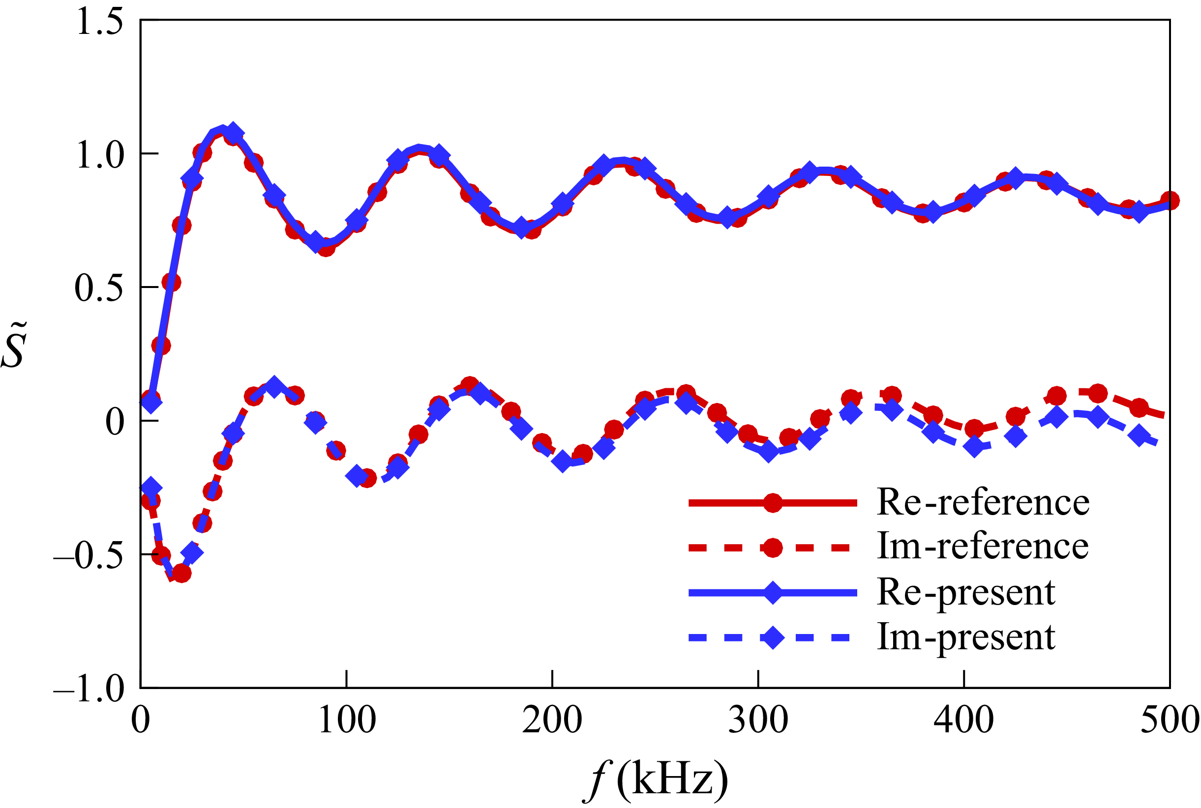


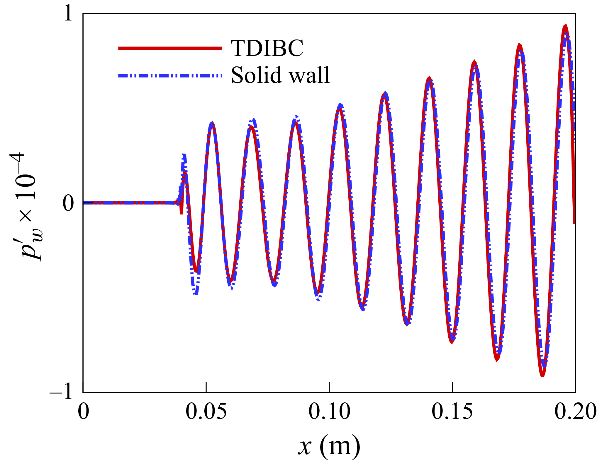


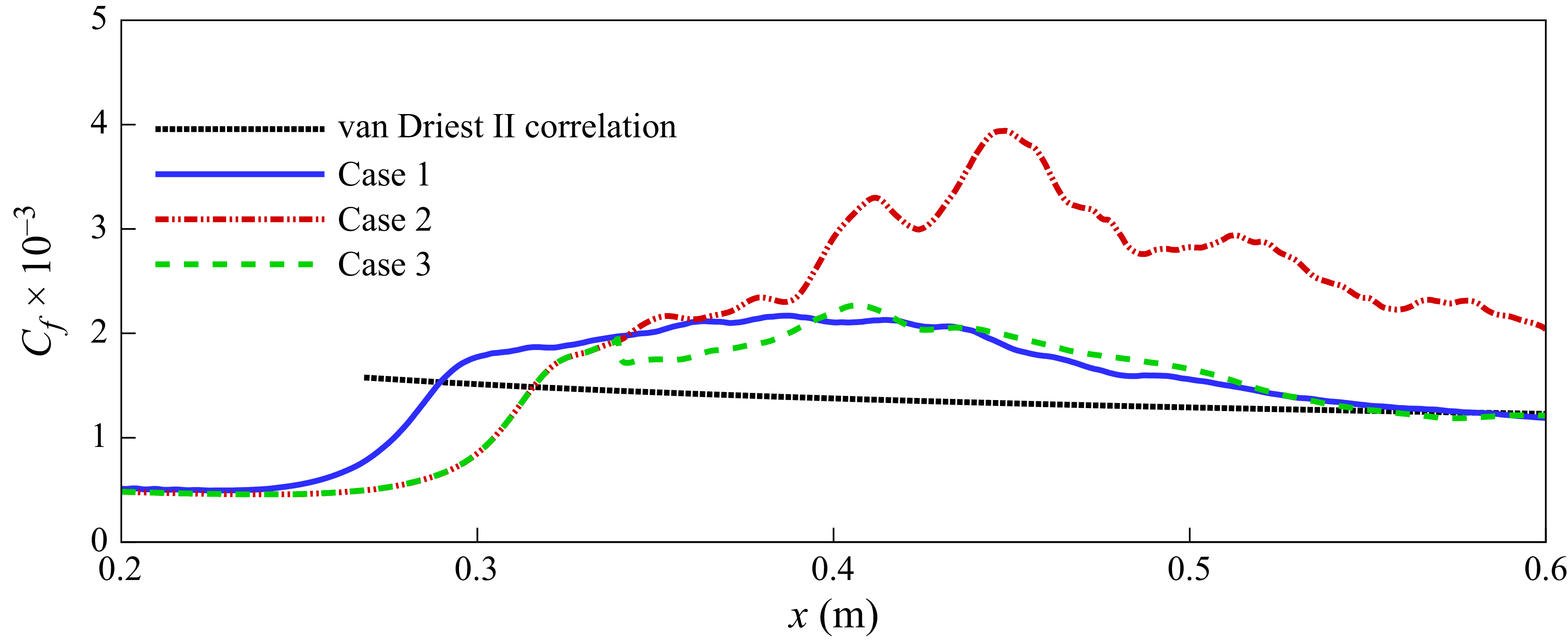


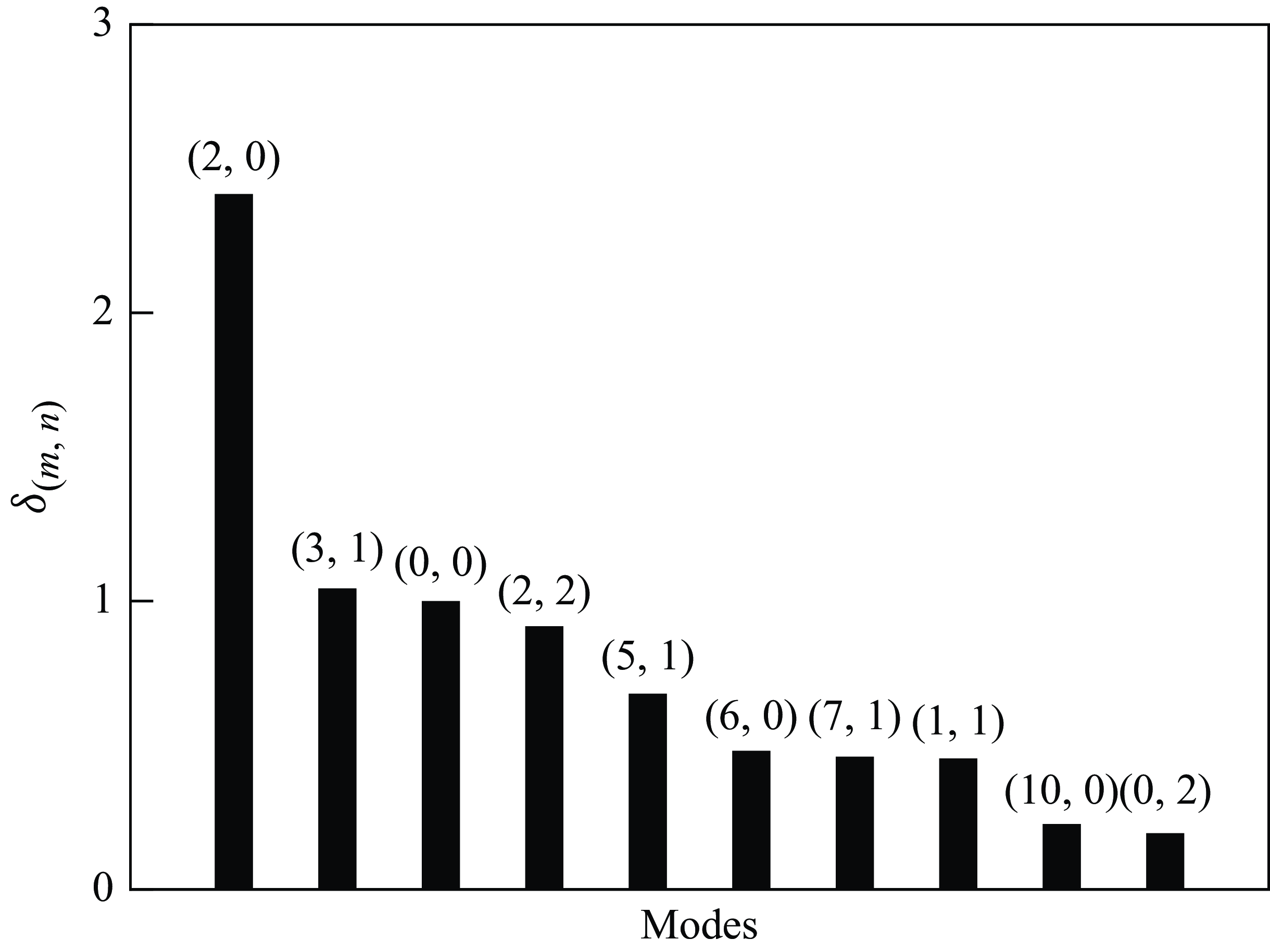


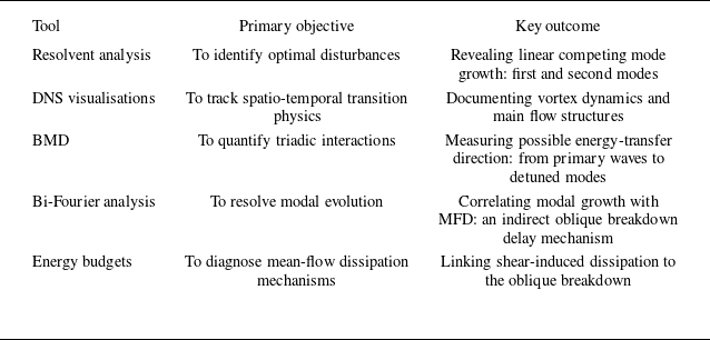
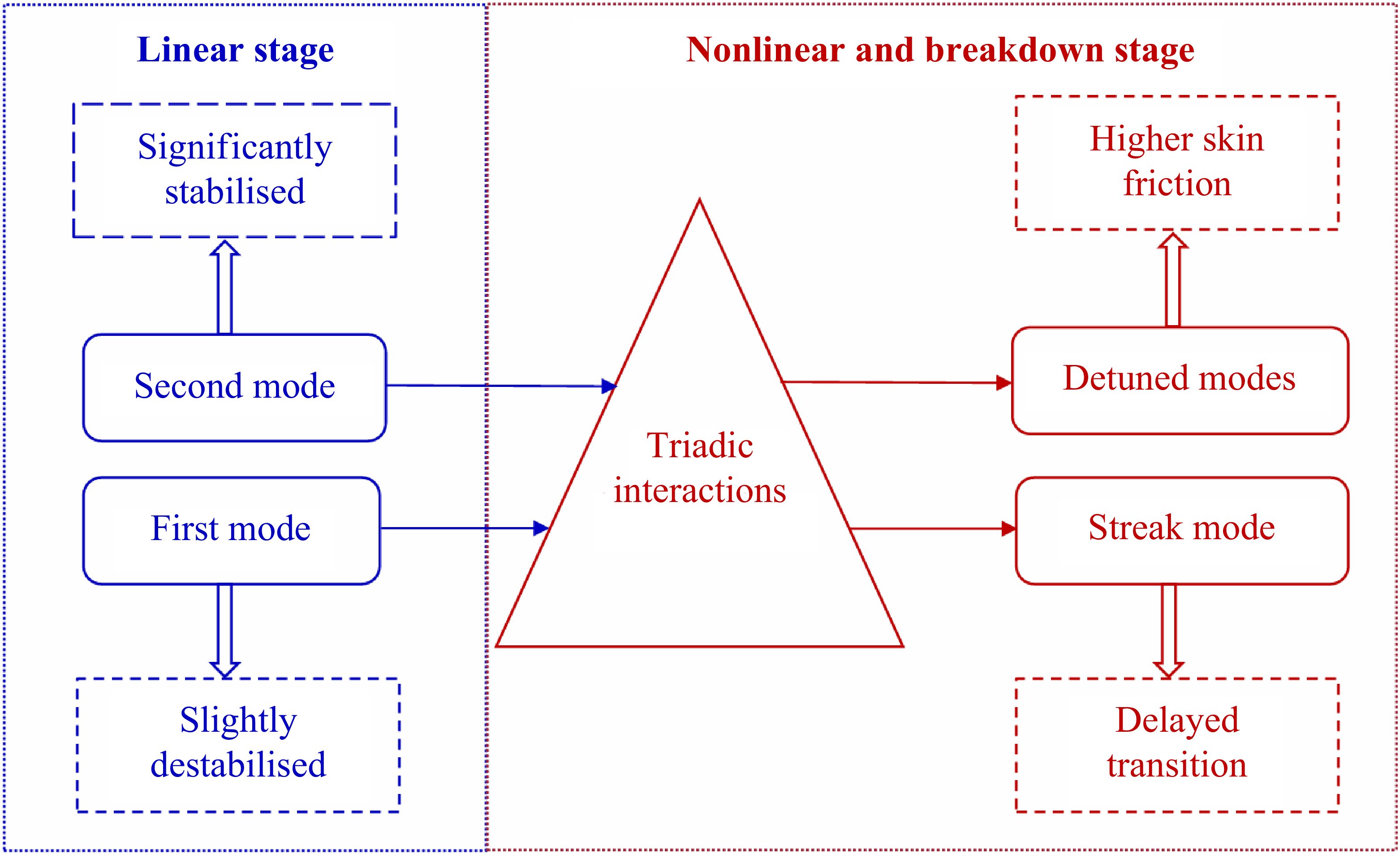
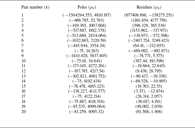
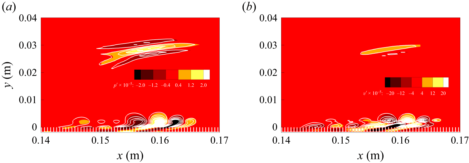


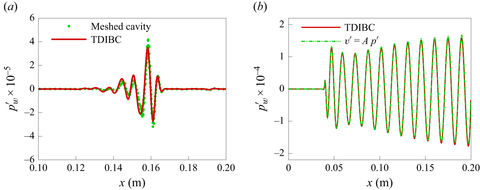


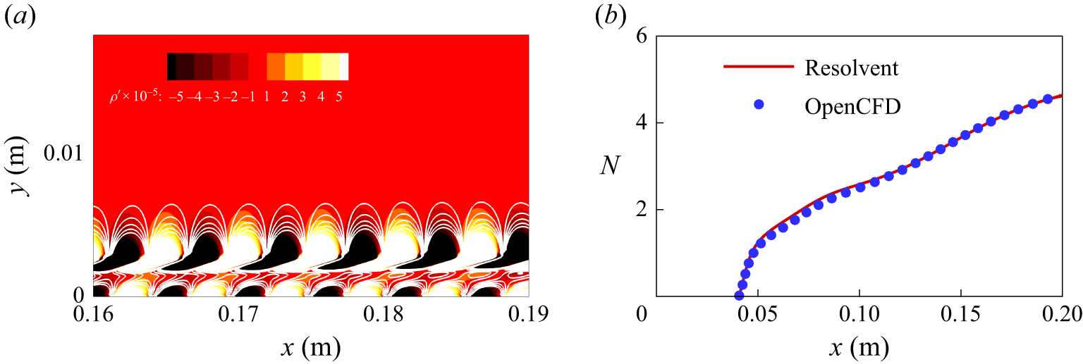


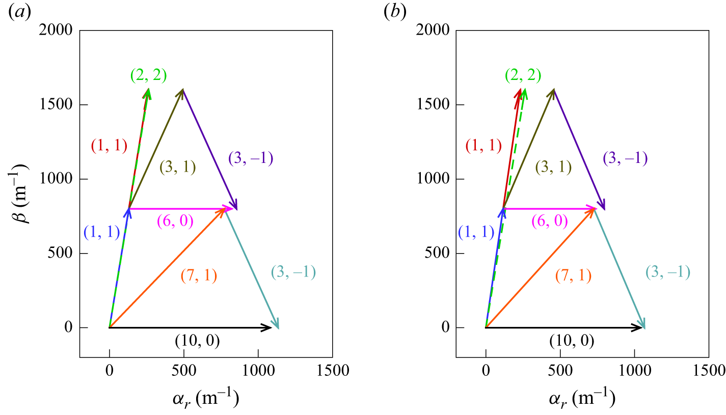


 Open access

