3.1. Qualitative behaviour of the multiphase flow

We start our discussion by looking at the qualitative structure of the flow in the statistically steady state that develops when the initial transient – required to absorb the initial conditions – is finished. Figure 1 shows a map of the TKE, $\text {TKE}= u'_i u'_i/2$, on a cross-section of the channel ($y$–$z$) located at $x=L_x/2$. Each panel refers to a different case: single phase (a), $\lambda =0.25$ (b), $\lambda =0.50$ (c), $\lambda =1.00$ (d), $\lambda =2.00$ (e) and $\lambda =4.00$ (f). The position of the interface (iso-level $\phi =0$) is indicated by a white line.

Figure 1.

Contour plot of turbulent kinetic energy (TKE) on a cross-section of the channel ($y$–$z$) located at $x=L_x/2$. Each panel refers to a different case: (a), single phase; (b), $\lambda =0.25$; (c), $\lambda =0.50$; (d), $\lambda =1.00$; (e), $\lambda =2.00$, (f), $\lambda =4.00$. The position of the interface is explicitly rendered via the thin white line. The different flow behaviour inside the thin lubricating layer, ranging from sustained turbulence ($\lambda <1$) to completely suppressed turbulence ($\lambda >1$), can be appreciated.

The qualitative results presented here confirm and extend our previous observations (Roccon et al. Reference Roccon, Zonta and Soldati2019). To discuss the flow modifications induced by the thin lubricating layer on the overall flow behaviour, we conveniently keep the single-phase case (figure 1a), for which classical near-wall turbulence structures are observed near the top and bottom boundaries, as reference. We immediately observe that, for all the viscosity stratified cases, the symmetry about the channel centre is broken, and the top and bottom boundaries behave differently based on the specific value of $\lambda$. We will focus on the bottom wall first, on the top wall later.

At the bottom wall ($z/h=-1$) the turbulence structure for all viscosity stratified cases (figure 1b–f) is similar to that of the single-phase case (figure 1a). The thin lubricating layer is too far to influence the near-wall turbulence regeneration cycle at the bottom wall (Lam & Banerjee Reference Lam and Banerjee1992; Jiménez Reference Jiménez2013). Nevertheless, a slight enhancement of the turbulence activity is observed for $\lambda =0.25$, $\lambda =0.50$ and $\lambda =1.00$. We anticipate here, but it will become clear later by looking at the fluid statistics, that this increase can be traced back to the larger gradients of the mean velocity profile and to the associated enhancement of the TKE production (Mansour, Kim & Moin Reference Mansour, Kim and Moin1988; Zonta et al. Reference Zonta, Marchioli and Soldati2012a).

At the top wall the situation is completely different and depends on the specific value of $\lambda$. For ease of discussion, we focus first on $\lambda =1.00$. Results for this case, which are given in figure 1(d), clearly show that turbulence is almost completely suppressed in the lubricating layer. This result, which confirms the observations made in our previous work (Roccon et al. Reference Roccon, Zonta and Soldati2019), can be directly attributed – as will be shown below – to the lubricating layer being too thin (or, alternatively to the local Reynolds number being too small) to sustain the near-wall turbulence cycle (Jiménez & Moin Reference Jiménez and Moin1991; Jiménez & Pinelli Reference Jiménez and Pinelli1999; Jiménez Reference Jiménez2013; Roccon et al. Reference Roccon, Zonta and Soldati2019). From a physical viewpoint, turbulence suppression is in this case due to the presence of the liquid–liquid interface – an elasticity element with the corresponding surface tension – that limits the wall-normal vertical transport of momentum and decouples the dynamics of the primary layer from that of the lubricating layers, which is then too thin to sustain turbulence itself. Mild velocity fluctuations might appear occasionally, and are induced by the motion of the liquid–liquid interface. The turbulence suppression process observed in the lubricating layer for $\lambda = 1.00$ appears magnified for $\lambda \ge 1$ (figure 1e,f), since the effect of the larger viscosity of the lubricating layer sums up with the action of the surface tension forces (Roccon et al. Reference Roccon, De Paoli, Zonta and Soldati2017). By contrast, for $\lambda =0.25$ and $\lambda =0.50$ (figure 1b,c), the viscosity in the lubricating layer is small enough – and the corresponding local Reynolds number large enough (Pecnik & Patel Reference Pecnik and Patel2017) – to sustain turbulence in the lubricating layer.

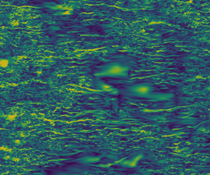
To appreciate better the different flow structures in the lubricating layer, we turn now our attention to the distribution of TKE on a $x-y$ horizontal plane located in the proximity of the top wall, at distance $d/h=0.03$. Results are shown in figure 2 and each panel refers to a different case: single phase (a), $\lambda =0.25$ (b), $\lambda =0.50$ (c) and $\lambda =1.00$ (d). Note that results for $\lambda =2.00$ and $\lambda =4.00$ are not shown since velocity fluctuations are largely suppressed and are therefore not visible. For the single-phase case (figure 2a), we recover the classical near-wall turbulence structure in which elongated high and low speed streaks appear side by side and line up along the streamwise direction (Lam & Banerjee Reference Lam and Banerjee1992; Schoppa & Hussain Reference Schoppa and Hussain2002; Chernyshenko & Baig Reference Chernyshenko and Baig2005). The picture changes quite significantly for the lubricated channel. In particular, for $\lambda =1.00$ (figure 2d), we see no evidence of turbulence activity, as turbulence is almost completely suppressed by the presence of the interface (Verschoof et al. Reference Verschoof, van der Veen, Sun and Lohse2016; Roccon et al. Reference Roccon, Zonta and Soldati2019). For $\lambda =0.25$ and $\lambda =0.50$ (figure 2b,c) turbulence appears reactivated in the lubricating layer. Yet, compared to the single-phase case, turbulence is less homogeneous, with the presence of banded structures of turbulent–laminar patches closely recalling those observed in other important flow instances (for example in thermally stratified turbulence, see García-Villalba & Del Álamo Reference García-Villalba and Del Álamo2011; Zonta, Onorato & Soldati Reference Zonta, Onorato and Soldati2012b; Zonta & Soldati Reference Zonta and Soldati2018). The coexistence of turbulent and laminar patches seems to be due to the deformation of the underneath interface separating the primary and the lubricating layer: crests and troughs (see appendix C for details) that naturally develop at the interface sometimes make the lubricating layer thin enough to locally suppress the turbulence activity. As a side observation – but we will not further comment on it – we report the change of size of turbulence structures at the wall, which appear smaller for smaller viscosity (i.e. larger local Reynolds number).

Figure 2.

Contour plot of TKE on a $x-y$ plane located at $z/h=0.97$ (i.e. taken inside the lubricating layer, at a distance $d/h=0.03$ from the top wall). (a) Refers to the single-phase case, (b) to the case $\lambda =0.25$, (c) to $\lambda =0.50$ and (d) to $\lambda =1.00$.

From a quantitative viewpoint, the presence of two distinct flow regimes (laminar/turbulent) in the lubricating layer can be justified using a semi-local scaling (Pecnik & Patel Reference Pecnik and Patel2017; Roccon et al. Reference Roccon, Zonta and Soldati2019) and computing the thickness of the lubricating layer in wall units (w.u.)

(3.1)\begin{equation} h_1^+=h_1 \frac{Re_\tau}{\lambda} \sqrt{\frac{2 |\tau_{w,1}|}{|\tau_{w,1}| + |\tau_{w,2}|}}, \end{equation}

where $h_1$ is the lubricating layer thickness in outer units, $Re_\tau$ is the equivalent shear Reynolds number (approximately $300$ here) and $\tau _{w,1}$ and $\tau _{w,2}$ are the wall-shear stresses at the top and bottom wall, respectively. In the present case, $h_1^+\simeq 30$ w.u. for $\lambda =1.00$, while it increases up to $h_1^+= 138$ w.u. for $\lambda =0.25$. These results suggest that the lubricating layer is too small to sustain turbulence for $\lambda =1.00$, whereas it becomes large enough to sustain turbulence for $\lambda <1$. Note that Jiménez & Pinelli (Reference Jiménez and Pinelli1999) established that the minimum dimensionless channel height to maintain a self-sustained near-wall turbulence cycle is $h^+\simeq 60$ w.u.

3.2. Flow rates and pressure gradient

The qualitative flow changes observed above naturally reflect into corresponding changes of the macroscopic flow parameters. Here, we focus on the time-averaged flow rate through the entire cross-section, $[Q_t]$, on the time-averaged flow rate of the primary layer, $[Q_2]$, and on the time-averaged mean pressure gradient, $[p_x]$. These results, which are represented in figure 3, are normalized by the corresponding values for the single-phase case, $[Q_{sp}]$ and $[p_{x}^{sp}]$, respectively. The region coloured in light grey in the diagram refers to flow configurations for which the viscosity of the lubricating layer is smaller than that of the primary layer (i.e. $\lambda <1$), while the region coloured in dark grey refers to flow configurations for which the viscosity of the lubricating layer is larger than that of the primary layer (i.e. $\lambda > 1$).

Figure 3.

Volume flow rate through the entire channel $[Q_t]$ (filled circles), volume flow rate of the primary layer $[Q_2]$ (empty circles), and mean pressure gradient $[p_x]$ (filled squares) as a function of the viscosity ratio $\lambda$. All results are normalized by the corresponding single-phase value. Note the non-monotonic behaviour of the different quantities which, for the cases here tested, reach an optimum (maximum flow rates and minimum pressure gradient, i.e. maximum DR) for $\lambda =1.00$. For $\lambda =4.00$, we report a marginal drag increase.

We immediately observe that, for $\lambda \leq 2.00$, $[Q_2]/[Q_{sp}]>1$ (empty circles) and $[Q_t]/[Q_{sp}]>1$ (filled circles). In other words, by keeping the applied power constant, the transferred flow rate is increased. This is a clear indication of DR, which is maximum for $\lambda =1.00$ (${\simeq }13\,\%$ of flow-rate increase), and is only slightly reduced for $\lambda = 0.50$ and $\lambda = 0.25$ (${\simeq }11\,\%$ of flow-rate increase). The reduction appears more intense for $\lambda = 2.00$ (${\simeq }5\,\%$ of flow-rate increase). When the viscosity of the lubricating layer is increased beyond $\lambda > 2$, we observe a drop of the flow rate that, giving $[Q_2]/[Q_{sp}]< 1$ for $\lambda = 4.00$ (${\simeq }5\,\%$ of flow-rate decrease), marks the occurrence of a drag increase.

Consistently with the previous observations, for $\lambda \leq 2.00$ the normalized pressure gradient is $[p_{x}]/[p_{x}^{sp}]<1$, so as to balance the increased flow rate and to keep the total power – product between the flow rate and the applied pressure gradient, in physical units – constant. The pressure gradient, which attains a minimum for $\lambda = 1.00$ ($[p_{x}]/[p_{x}^{sp}]\simeq 0.86$), increases only slightly for $\lambda <1$ ( $[p_{x}]/[p_{x}^{sp}]\simeq 0.9$ for $\lambda = 0.5$ and $\lambda = 0.25$); on the other hand, it increases more vigorously for $\lambda >1$, up to the point at which, for $\lambda = 4.00$, it becomes slightly larger than unity.

Note that, since simulations are performed at slightly different power Reynolds numbers (see table 1), the product between the total flow rate and the mean pressure gradient, which is by construction constant in physical units, is slightly different when considered in dimensionless units.

3.3. Mean velocity profiles

Linked to the previous analysis on the flow-rate and pressure gradient modulations in the lubricated channel, we focus now on the behaviour of the mean streamwise velocity profile, $[ u_x ]$, as a function of the wall-normal coordinate. Results are shown in figure 4 according to the following colour code: red is used for $\lambda =0.25$, yellow for $\lambda =0.50$, green for $\lambda =1.00$, light blue for $\lambda =2.00$ and dark blue $\lambda =4.00$. The single-phase case is represented by the thin black line, while the reference position of the interface ($z/h=0.85$) is identified by the vertical dashed black line. As expected, the shape of the mean velocity profile appears skewed by the presence of the liquid–liquid interface.

Figure 4.

Wall-normal behaviour of the mean streamwise velocity, $[ u_x ]$. The different cases of lubricated channel considered in the present study are reported using different colours: $\lambda =0.25$ (red), $\lambda =0.50$ (yellow), $\lambda =1.00$ (green), $\lambda =2.00$ (blue) and $\lambda =4.00$ (dark blue). The single-phase case (thin black line) is also shown for reference. The nominal position of the interface ($z/h=0.85$) is given by a dashed vertical black line.

In the primary layer, and consistently with the previous analysis on the overall flow rate, the behaviour of $[ u_x ]$ is non-monotonic and is maximized for $\lambda =1.00$. A reduction of the viscosity ratio from $\lambda =1.00$ to $\lambda =0.50$ and $\lambda =0.25$ – which almost overlap – induces only a small decrease of $[ u_x ]$. On the other hand, an increase of $\lambda$ beyond unity, $\lambda > 1.00$, produces stronger modification. For $\lambda = 2.00$, the mean velocity profile appears largely reduced – although in any case well above the single-phase limit – compared to $\lambda =1.00$. Moving to $\lambda = 4.00$, we reach a condition at which the velocity profile is very close to that of the single-phase case in a large proportion of the primary layer, but suddenly drops in the proximity of the interface.

In the lubricating layer, $0.85 < z/h < 1.00$, the trend of the mean velocity turns out to be monotonic with the viscosity ratio $\lambda$: $[u_x]$ increases consistently with decreasing $\lambda$. A similar behaviour characterizes the mean velocity gradient that, being minimum for $\lambda =4.00$ and maximum for $\lambda =0.25$, reflects the different flow structure in the lubricating layer – with turbulence progressively suppressed for increasing $\lambda$ (see also figures 1 and 2). To have a classical view of the velocity profiles, they must be rescaled with the local friction velocity (i.e. evaluated at the corresponding wall). This comparison is offered in appendix D.

3.4. Energy box: preliminary concepts

To provide a sound characterization of the energy fluxes in the lubricated channel, we decide to use the so-called energy-box technique (Ricco et al. Reference Ricco, Ottonelli, Hasegawa and Quadrio2012; Gatti et al. Reference Gatti, Cimarelli, Hasegawa, Frohnapfel and Quadrio2018). This technique, starting from the mean and TKE balance equations, provides a thorough and meaningful representation of the energy fluxes in the system. Note that, and precisely because of the adoption of a CPI approach, all simulations are performed driving the system with the same physical power input $P_p$. Therefore, a direct comparison between the different cases is possible (Hasegawa et al. Reference Hasegawa, Quadrio and Frohnapfel2014).

To compute the energy budget, the total kinetic energy of the flow is decomposed into mean kinetic energy (MKE), $\text {MKE}=\frac {1}{2}\langle u_i \rangle \langle u_i \rangle$, and TKE, $\text {TKE} =\frac {1}{2}u'_i u'_i$. In the following, and building on top of the MKE and TKE definitions, we will present and discuss the energy-box technique for single and multiphase flows.

3.5. Energy box for a single-phase flow

The starting points of the energy-box technique are the MKE and TKE transport equations, obtained multiplying the Navier–Stokes equations by the mean velocity field – MKE balance equation – and by the fluctuating velocity field – TKE balance equation (Mansour et al. Reference Mansour, Kim and Moin1988; Kasagi, Tomita & Kuroda Reference Kasagi, Tomita and Kuroda1992; Iwamoto, Suzuki & Kasagi Reference Iwamoto, Suzuki and Kasagi2002). For the reference single-phase case, the ensemble average balance equation for the MKE becomes

(3.2)\begin{align} \frac{\textrm{D} [ \text{MKE} ]}{\textrm{D} t}&= \underbrace{ - [ \langle u_i \rangle \langle p_x \rangle ]}_{\varPi_m} +\underbrace{ \left[ \langle u'_i u'_j \rangle \frac{\partial \langle u_i \rangle }{\partial x_j} \right]}_{P_k} -\underbrace{ \left[ \frac{\partial (\langle u'_i u'_j \rangle \langle u_i \rangle) }{\partial x_j} \right]}_{T_m} \nonumber\\ &\quad +\underbrace{\left[ \frac{1}{2Re_{\varPi}} \frac{\partial^2 \langle u_i \rangle^2 }{\partial x_j^2} \right]}_{D_m} \underbrace{ - \left[ \frac{1}{Re_{\varPi}} \frac{\partial \langle u_i \rangle}{\partial x_j}\frac{\partial \langle u_i \rangle}{\partial x_j} \right]}_{\epsilon_m}, \end{align}

where $\langle u'_i u'_j \rangle$ are the Reynolds stresses. While the left-hand side represents the material rate of change of MKE, the different terms on the right-hand side represent the power injected in the system via the mean pressure gradient, $\varPi _m$, the production of TKE, $P_k$, the work done by the Reynolds stresses, $T_m$, the viscous diffusion of MKE, $D_m$, and the mean flow viscous dissipation, $\epsilon _m$.

The ensemble-averaged balance equation for the TKE reads as

(3.3)\begin{align} \frac{\textrm{D} [ \text{TKE} ]}{\textrm{D} t}&= \underbrace{- \left[ \frac{ \partial \langle p'u'_i \rangle}{\partial x_i} \right]}_{\varPi_k} -\underbrace{ \left[ \langle u'_i u'_j \rangle \frac{\partial \langle u_i \rangle }{\partial x_j} \right]}_{P_k} \underbrace{- \left[ \frac{1}{2}\frac{\partial \langle u'_i u'_i u'_j \rangle }{\partial x_j} \right]}_{T_k} \nonumber\\ &\quad +\underbrace{\left[ \frac{1}{2Re_{\varPi}} \frac{\partial^2 \langle u'_i u'_i \rangle}{\partial x_j^2} \right]}_{D_k} \underbrace{- \left[ \frac{1}{Re_{\varPi}} \frac{\partial u'_i }{\partial x_j}\frac{\partial u'_i }{\partial x_j} \right]}_{\epsilon_k}. \end{align}

The left-hand side represents the material rate of change of TKE. The terms on the right-hand side represent the pressure diffusion, $\varPi _k$, the production of TKE, $P_k$, the turbulent diffusion, $T_k$, the viscous diffusion of TKE, $D_k$, and the turbulent viscous dissipation, $\epsilon _k$.

We can now proceed to discuss the different terms of each equation from a physical point of view. For (3.2) – MKE balance – the left-hand side is zero, since the flow is statistically steady. On the right-hand side, the power input, $\varPi _m$, is a source term and represents the power injected in the system via the mean pressure gradient. This power is then partially dissipated by the mean flow viscous dissipation, $\epsilon _m$, and partially used to generate turbulent fluctuations via the production term, $P_k$. Therefore, $\epsilon _m$ and $P_k$ represent a sink of energy in the MKE balance equation. The two remaining terms, the energy transport by the Reynolds stress, $T_m$, and the viscous diffusion, $D_m$, redistribute the energy across the channel and thus act only as internal transport mechanisms that do not bear a net contribution. In other words, they are neither sinks nor sources.

Considering (3.3) – TKE balance – the left-hand side is also zero, always in light of the statistically steady condition. On the right-hand side, the TKE production term, $P_k$, accounts for the generation of velocity fluctuations via mean shear. This term, which was a sink in the MKE equation, represents a source in the TKE equation. The power injected via $P_k$ is entirely dissipated by the turbulent dissipation, $\epsilon _k$, which is the only sink term in (3.3). The pressure diffusion, $\varPi _k$, the turbulent diffusion, $T_k$, and the viscous diffusion, $D_k$, are redistribution terms with no net contribution.

To evaluate the overall importance of the different terms, we compute the integral of the two balance equations along the wall-normal direction. With reference to a generic term $A_{m/k}$, and using an overbar to indicate the integral over the wall-normal direction $z$, we obtain

(3.4)\begin{equation} \overline{A_{m/k}}=\int^{z/h=+1}_{z/h=-1} [A_{m/k} ]\, \textrm{d} z .\end{equation}

Clearly, this integral is zero for the internal transport (redistribution) terms, while it is positive (respectively negative) for the source (respectively sink) terms. Therefore, the integral counterparts of the MKE and TKE balance equations, (3.2) and (3.3), read as

(3.5)\begin{gather} \overline{{P}_k} + \overline{\varPi_m}+ \overline{\epsilon_m} =0 , \end{gather}

(3.6)\begin{gather}- \overline{{P}_k}+ \overline{\epsilon_k}=0 , \end{gather}

respectively. Combining (3.5) and (3.6), we obtain a balance equation for the total kinetic energy

(3.7)\begin{equation} \overline{\varPi_m}+\overline{\epsilon_m} + \overline{\epsilon_k}=0 ,\end{equation}

which states that the entire power injected into the system, $\overline {\varPi _m}$, is ultimately dissipated by viscosity, both via the viscous dissipation term of the mean field, $\overline {\epsilon _m}$, and via the viscous dissipation term of the fluctuating field, $\overline {\epsilon _k}$. We can now visualize the energy fluxes in the present configuration using the energy-box representation, as shown in figure 5.

Figure 5.

Energy-box representation for the single-phase reference case. The left box represents the MKE of the flow, while the right box identifies the TKE of the flow. Each arrow refers to a different energy flux, whose magnitude is normalized by the value of the injected power, $\overline {\varPi _m}$, represented by a green arrow. The mean flow viscous dissipation, $\overline {\epsilon _m}$, and the turbulent dissipation, $\overline {\epsilon _k}$, are represented by a red arrow – leaving the left and right box, respectively – while the TKE production, $\overline {P_k}$, is represented by a blue arrow.

The two adjacent boxes represent the MKE (left) and TKE (right) content of the flow, respectively. Arrows are used to represent energy source (green), energy exchange (blue) and energy sink (red). The magnitude of each contribution, normalized by the power input, is given near the corresponding arrow. By looking at the left box, it is apparent that the applied power, $\overline {\varPi _m}$, which is injected into the mean flow (MKE), is in part (${\simeq }54\,\%$) dissipated by the mean flow itself, $\overline {\epsilon _m}$, and in part (${\simeq }46\,\%$) transferred to TKE, $\overline {P_k}$. The power transferred to TKE is then dissipated by turbulent dissipation, $\overline {\epsilon _k}$. When lumped together, the MKE and TKE boxes represent the energy balance of the total kinetic energy, (3.7).

3.6. Energy box for the lubricated channel

We now extend the energy-box representation to the case of a lubricated channel. As done before, to derive the modified energy balance equations, we multiply the Navier–Stokes equations by the mean and fluctuating velocity field and we average the resulting equations in space and time. For the MKE, we get

(3.8)\begin{align} \frac{\textrm{D} [ \text{MKE} ]}{\textrm{D} t}&= \underbrace{ \left[ \langle u'_i u'_j \rangle \frac{\partial \langle u_i \rangle }{\partial x_j} \right]}_{P_k} \underbrace{ - [ \langle u_i \rangle \langle p_x \rangle ]}_{\varPi_m} -\underbrace{ \left[ \frac{\partial (\langle u'_i u'_j \rangle \langle u_i \rangle) }{\partial x_j} \right]}_{T_m} \nonumber\\ & \quad +\underbrace{\left[ \frac{1}{2Re_{\varPi}} \frac{\partial }{\partial x_j} \left( \langle \eta (\phi) \rangle \frac{\partial \langle u_i \rangle^2}{\partial x_j} \right) \right]}_{D_m} \underbrace{ - \left[ \frac{\langle \eta (\phi) \rangle}{Re_{\varPi}} \frac{\partial \langle u_i \rangle}{\partial x_j}\frac{\partial \langle u_i \rangle}{\partial x_j} \right]}_{\epsilon_m} \nonumber\\ & \quad +\underbrace{\left[ \langle u_i \rangle \frac{3 Ch}{\sqrt{8} We_\varPi} \frac{\partial \langle \tau^c_{ij} \rangle }{\partial x_j} \right]}_{\psi_m} , \end{align}

where we can observe the appearance of an additional term, $\psi _m$, which represents the work of the surface tension forces on the mean flow.

For the TKE, we get

(3.9)\begin{align} \frac{\textrm{D} [ \text{TKE} ]}{\textrm{D} t}&= -\underbrace{ \left[ \langle u'_i u'_j \rangle \frac{\partial \langle u_i \rangle }{\partial x_j} \right]}_{P_k} \underbrace{- \left[ \frac{ \partial \langle p'u'_i \rangle}{\partial x_i} \right]}_{\varPi_k} \underbrace{- \left[ \frac{1}{2}\frac{\partial \langle u'_i u'_i u'_j \rangle }{\partial x_j} \right]}_{T_k} \nonumber\\ &\quad +\underbrace{\left[ \frac{1}{2Re_{\varPi}} \frac{\partial }{\partial x_j} \left( \eta (\phi) \frac{\partial \langle u'_i u'_i \rangle}{\partial x_j} \right) \right]}_{D_k} \underbrace{- \left[ \frac{\eta(\phi)}{Re_{\varPi}} \frac{\partial u'_i }{\partial x_j}\frac{\partial u'_i }{\partial x_j} \right]}_{\epsilon_k} +\underbrace{\left[ u'_i \frac{3 Ch}{\sqrt{8} We_\varPi} \frac{\partial \tau'^{c}_{ij}}{\partial x_j} \right]}_{\psi_k} . \end{align}

Even in this case, there is an additional term, $\psi _k$, which represents the work exchanged, via the surface tension forces, between the interface and the fluctuating field (Li & Jaberi Reference Li and Jaberi2009).

To derive the macroscopic balance equations for the lubricate channel and hence to set the corresponding energy-box representation, we integrate over the wall-normal direction the obtained MKE/TKE balance equations. For the MKE, we have

(3.10)\begin{equation} \overline{{P}_k} + \overline{\varPi_m}+ \overline{\epsilon_m} + \overline{\psi_m} =0 ,\end{equation}

while for the TKE, we have

(3.11)\begin{equation} - \overline{{P}_k}+ \overline{\epsilon_k} + \overline{\psi_k}=0 .\end{equation}

At this point, it is worth further elaborating on the energetics associated with the presence of an interface – an elasticity element – inside the flow. Following Joseph (Reference Joseph1976, p. 242), and under the assumption of constant and uniform surface tension, we can obtain an energy balance equation for the liquid–liquid interface (see appendix E for details)

(3.12)\begin{equation} -\frac{1}{L_x L_y} \frac{1}{We_{\varPi}} \left[ \frac{\textrm{d} A}{\textrm{d} t } \right]=\overline{\psi_m} + \overline{\psi_k} =0, \end{equation}

which states that an increase of the interfacial area (i.e. an increase of the interfacial energy) must correspond to a negative work of the surface tension forces (i.e. velocity and surface tension forces act in opposite directions). In statistically steady state conditions, the average value of the interfacial area remains constant and thus

(3.13)\begin{equation} \overline{\psi_m} + \overline{\psi_k} =0,\end{equation}

indicating that the total power – sum of mean and fluctuating contributions – absorbed/released by the surface tension forces is null (Joseph Reference Joseph1976; Aris Reference Aris1989; Dodd & Ferrante Reference Dodd and Ferrante2016). Equation (3.13) highlights the pure elastic behaviour of the interface and thus the absence of net energy dissipation associated with its deformation. Combining (3.13) with (3.10) and (3.11), we get the balance equation for the total kinetic energy

(3.14)\begin{equation} \overline{\varPi_m}+\overline{\epsilon_m} + \overline{\epsilon_k}=0 .\end{equation}

Therefore, very much like the TKE production term, surface tension forces act as a transfer of energy between MKE and TKE. We anticipate here that the surface tension contribution is a sink term in the MKE equation, and a source term in the TKE equation. However, it must be also mentioned that as customary when a one-fluid approach is employed to analyse a multiphase system (Prosperetti & Tryggvason Reference Prosperetti and Tryggvason2009; Popinet Reference Popinet2018), and precisely because the surface tension forces are smeared out on a thin interfacial layer, the two interfacial contributions do not exactly match and $|\overline {\psi _{m}}| \geq |\overline {\psi _{k}}|$. Nevertheless, for the cases presented here, this difference is always smaller (in the worst condition) than $0.4\,\%$ of the total power injected in the system. For ease of notation, in the energy-box representation reported below, the surface tension contribution is conventionally identified by the value of $\overline {\psi _{m}}$. A mechanistic view of the role of the surface tension forces on the energy transfer between the main and the lubricating layer is given in appendix F.

The energy-box representation for the lubricated channel is shown in figure 6. Each panel refers to a different viscosity ratio: $\lambda =0.25$ (a), $\lambda =1.00$ (b) and $\lambda =4.00$ (c). The results for $\lambda =0.50$ and $\lambda =2.00$ are not shown since they represent only intermediate cases that do not add to the discussion. As set above, source terms are represented by green arrows, transport terms by blue arrows and sink terms by red arrows. The additional contribution of the interfacial terms is rendered by a yellow arrow connecting the MKE box to the TKE box via an additional box that represents the interface and its dynamics – an elastic component absorbing and releasing energy.

Figure 6.

Ensemble-averaged energy box for the different cases of the lubricated channel: $\lambda =0.25$ (a), $\lambda =1.00$ (b) and $\lambda =4.00$ (c). Note that $\lambda =0.50$ and $\lambda =2.00$ are not shown since they do not add to the present discussion. The left box refers to the MKE of the flow while the right box refers to the TKE of the flow. The power injected into the system, $\overline {\varPi _m}$, is represented by a green arrow. The mean flow viscous dissipation, $\overline {\epsilon _m}$, is represented by a red arrow (left box); the TKE production, $\overline {P_k}$, and the surface tension contribution, $\overline {\psi _{m}}$, are represented by a blue and a yellow arrow, respectively. Finally, the turbulent dissipation, $\overline {\epsilon _k}$, is represented by a red arrow (right box).

We will discuss the case $\lambda =1.00$ (figure 6b) first, the case $\lambda =0.25$ (figure 6a) and $\lambda =4.00$ (figure 6c) later. This strategy helps explicating the impact of surface tension and viscosity ratio on the energy fluxes in a more systematic way, focusing on the contribution of each single property one independently to each other. For $\lambda =1.00$, and compared to the single-phase case, we observe an increase of the mean flow viscous dissipation, $\overline {\epsilon _m}$, from 54 % up to 58 %. This result indicates that the reduced velocity gradients in the lubricating layer, which are due to the documented turbulence suppression therein (see § 3.1), are completely compensated by the increased velocity gradients at the bottom wall.

In addition, and precisely because of the observed turbulence suppression in the lubricating layer, we notice a significant decrease of TKE production, $\overline {P_k}$, which goes from 46 % (single phase) down to 39 % ($\lambda =1.00$). The contribution of the surface tension forces, $\overline {\psi _{m}}$, is in this case rather small (${\simeq }2\,\%$). The sum of the TKE production and of the interfacial contribution gives the amount of power used to generate TKE, which is ultimately dissipated via turbulent dissipation, $\overline {\epsilon _k}$. Examined under this perspective, the DR turns out to be induced by the surface tension forces that, blocking the wall-normal transfer of momentum, promote the laminarization of the lubricating layer (which is characterized by a small thickness, hence a small local Reynolds number) and induce a sharp decrease of the overall turbulence production. As a consequence, the power injected in the system is more efficiently used to drive the motion of the two liquid layers.

Moving to $\lambda =0.25$ (figure 6a), we now observe remarkable differences. The mean flow viscous dissipation, $\overline {\epsilon _m}$, reduces to 48 %, while the TKE production increases up to 49 %. Accordingly, and considering that the contribution of the interfacial term, $\overline {\psi _{m}}$, remains rather small (${\simeq }3\,\%$), we notice a corresponding increase of the turbulent dissipation up to 51 %. Present results, reporting a decrease of $\overline {\epsilon _m}$ and an increase of $\overline {\epsilon _k}$, seem to be in contrast to the observed DR. Note indeed that, in the framework of the CPI approach and using passive DR techniques, DR is usually associated with an increase of $\overline {\epsilon _m}$ and a decrease of $\overline {\epsilon _k}$ (although, strictly speaking, this latter conclusion is based on the specific procedure used in Gatti et al. (Reference Gatti, Cimarelli, Hasegawa, Frohnapfel and Quadrio2018) to model the wall-normal behaviour of the wall-shear stress). To reconcile present results with previous predictions, an extended version of the energy-box technique –as will be discussed in § 3.8 – must be introduced.

For $\lambda =4.00$ (figure 6c), the energy box is similar to that observed for $\lambda =1.00$ (figure 6a), with an increase of the mean flow dissipation up to 57 %, and a decrease of the TKE production down to 38 % – again due to the turbulence suppression in the lubricating layer. Interestingly, we also report a slight increase of the contribution of the interfacial term, $\overline {\psi _{m}}$, which becomes ${\simeq }5\,\%$. This latter observation seems to be related to the dynamics of interfacial waves: when the viscosity of the lubricating layer is increased, the larger shear rate induces a larger deformation of the interface and this leads to a larger $\overline {\psi _{m}}$ (see also appendix F). The increase of $\overline {\psi _{m}}$ (in magnitude) is also reflected by the release of TKE near the interface: increasing the viscosity of the lubricating layer, the liquid–liquid interface becomes less and less compliant and behaves almost like a solid wavy interface that promotes the generation of velocity fluctuations (Breugem, Boersma & Uittenbogaard Reference Breugem, Boersma and Uittenbogaard2006; Rosti & Brandt Reference Rosti and Brandt2017) (see also the higher TKE levels close to the interface – on the primary layer side – shown in figure 1f). Overall, for $\lambda =4.00$, the analysis of the energy budgets seems to indicate DR (increasing $\overline {\epsilon _m}$ and decreasing $\overline {\epsilon _k}$), which it is in fact not observed in practice (see § 3.2).

Altogether, these results for $\lambda \ne 1$ show that the original energy-box technique, when applied straightforwardly to a multiphase flow, leads to conclusions which seem to be in contrast with previous findings (Gatti et al. Reference Gatti, Cimarelli, Hasegawa, Frohnapfel and Quadrio2018). To overcome these limitations, the energy-box technique must be extended – and a phase discrimination procedure must be included – to account for the multiphase nature of the system. This is the objective of the next sections.

3.7. Virtually lubricated channel

Before proceeding with the derivation of the phase-averaged approach applied to the lubricated channel, and precisely to evaluate a representative reference case against which current results can be conveniently compared, we introduce the concept of a virtually lubricated channel. A virtually lubricated channel is a single-phase flow that is a posteriori split – using a virtual interface located at a distance $0.15h$ far from the top wall. This virtual interface has no surface tension and therefore does not have any effects on the velocity field, since the flow is obtained by the solution of the Navier–Stokes equations in a single-phase system with uniform density and viscosity. The energy-box representation for the virtually lubricated channel is given in figure 7. Since the different terms refer now to a specific subregion of the domain (lubricating or primary layer), an additional subscript is used to distinguish between the virtual lubricating layer – subscript 1 – and the virtual primary layer – subscript 2 – contributions. Note also the presence of dark blue arrows, which identify the energy fluxes (transport/redistribution terms, referred to as $\overline {F_m}$ and $\overline {F_k}$) exchanged between the two virtual fluid layers – redistribution terms are indeed null only when integrated over the entire volume.

Figure 7.

Energy box for the virtually lubricated channel, namely a single-phase case virtually separated into a lubricating and a primary layer. The virtual separation is located at the nominal position of the interface (distance $0.15~\textrm {h}$ from top wall). The left dashed box represents the MKE of the flow while the right box represents the TKE of the flow. Inside each dashed box, the top and bottom rectangles identify the (virtual) lubricating and primary layers, respectively. Each arrow refers to a different energy flux, whose magnitude is reported (near the arrow) normalized by the power input value. Compared to the previous energy boxes (ensemble averaged), an additional subscript is used to distinguish between the lubricating and primary layer contributions. The power injected in the system, $\overline {\varPi _m}$, is represented by a green arrow; the mean flow viscous dissipations, $\overline {\epsilon _{m,1}}$ and $\overline {\epsilon _{m,2}}$, by red arrows (left), and the TKE production terms, $\overline {P_{k,1}}$ and $\overline {P_{k,2}}$, by blue arrows. Finally, the turbulent dissipations, $\overline {\epsilon _{k,1}}$ and $\overline {\epsilon _{k,2}}$, are represented with red arrows (right). Note the appearance of dark blue arrows, identifying energy fluxes exchanged between the primary and the lubricating layer, $\overline {F_m}$ and $\overline {F_k}$.

By looking at figure 7 we notice that the viscous dissipation of MKE has a similar value in both layers, $\overline {\epsilon _{m,1}}\simeq \overline {\epsilon _{m,2}}$, while there is a sharp difference in the viscous dissipation of TKE, $\overline {\epsilon _{k,1}} \ne \overline {\epsilon _{k,2}}$. This representation gives a clearcut idea of the energy that is transferred and dissipated in the region virtually corresponding to the primary layer of the channel, and favours the introduction of an energy transfer efficiency, which we conveniently define as

(3.15)\begin{equation} \mathcal{H}_{sp}=\frac{\overline{\epsilon_{m,2}}}{( \overline{\epsilon_{m,2}}+ \overline{\epsilon_{k,2}})}=0.456. \end{equation}

This parameter represents the ratio between the mean energy dissipation in the primary layer, and the total energy dissipation, i.e. after deduction of the energy transferred to the lubricating layer, in the primary layer.

In the following, we will make specific reference to this configuration.

3.8. Phase-averaged energy box for viscosity stratified flow

Based on the above discussion (see § 3.6), it is apparent that the original energy-box technique must be properly extended to analyse the case of a lubricated channel. Because of the multiphase nature of the flow, an averaging procedure applied to the entire volume – such as the one employed above – does not provide a separation between the primary and the lubricating layer contributions and, more importantly, does not grant access to the evaluation of the energy fluxes between these two layers.

To investigate these aspects, we compute the energy budget for each layer in isolation (Dodd & Ferrante Reference Dodd and Ferrante2016; Rosti et al. Reference Rosti, Ge, Jain, Dodd and Brandt2019). The obtained results are then represented in an opportunely modified energy box. To derive the phase-averaged MKE/TKE balance equations, we use the phase-field variable $\phi$ and we define a local concentration, $0 \le c_l \le 1$, for each liquid layer

(3.16a,b)\begin{equation} c_1=\frac{1+\phi}{2}, \quad c_2=\frac{1-\phi}{2}, \end{equation}

where, as anticipated before, the subscript $l=1,2$ is used to identify the lubricating and primary layer local concentrations, respectively. Multiplying MKE and TKE balance equations by the two local concentrations, and averaging in space ($x,y$) and in time as explained in § 3.6, we obtain the energy balance equations for each liquid layer. In particular, the phase-averaged MKE for each layer $l$, $[\text {MKE}]_l$ – counterpart of (3.8) – becomes

(3.17)\begin{align} \frac{\textrm{D} [ \text{MKE} ]_l}{\textrm{D} t}&= \underbrace{ \left[ c_l \langle u'_i u'_j \rangle \frac{\partial \langle u_i \rangle }{\partial x_j} \right]}_{P_{k,l}} \underbrace{ - \left[ c_l \langle u_i \rangle \left\langle p_x \right\rangle \right]}_{\varPi_{m,l}} -\underbrace{ \left[ c_l \frac{\partial (\langle u'_i u'_j \rangle \langle u_i \rangle) }{\partial x_j} \right]}_{T_{m,l}} \nonumber\\ &\quad +\underbrace{\left[ \frac{c_l}{2Re_{\varPi}} \frac{\partial }{\partial x_j} \left( \langle \eta (\phi) \rangle \frac{\partial \langle u_i \rangle^2}{\partial x_j} \right) \right]}_{D_{m,l}} \underbrace{ - \left[ c_l \frac{\langle \eta (\phi) \rangle}{Re_{\varPi}} \frac{\partial \langle u_i \rangle}{\partial x_j}\frac{\partial \langle u_i \rangle}{\partial x_j} \right]}_{\epsilon_{m,l}} \nonumber\\ &\quad +\underbrace{\left[ c_l \langle u_i \rangle \frac{3 Ch}{\sqrt{8}We_\varPi} \frac{\partial \langle \tau^c_{ij} \rangle}{\partial x_j} \right]}_{\psi_{m,l}} . \end{align}

Similarly, the phase-averaged TKE for each liquid layer $l$, $[\text {TKE}]_l$ – counterpart of (3.9) – becomes

(3.18)\begin{align} \frac{\textrm{D} [ \text{TKE} ]_l}{\textrm{D} t}&= -\underbrace{ \left[ c_l \langle u'_i u'_j \rangle \frac{\partial \langle u_i \rangle }{\partial x_j} \right]}_{P_{k,l}} \underbrace{- \left[ c_l \frac{ \partial \langle p'u'_i \rangle}{\partial x_i} \right]}_{\varPi_{k,l}} \underbrace{- \left[ \frac{c_l}{2}\frac{\partial \langle u'_i u'_i u'_j \rangle }{\partial x_j} \right]}_{T_{k,l}} \nonumber\\ &\quad +\underbrace{\left[ \frac{c_l}{2Re_{\varPi}} \frac{\partial }{\partial x_j} \left( \eta (\phi) \frac{\partial \langle u'_i u'_i \rangle}{\partial x_j} \right) \right]}_{D_{k,l}} \underbrace{- \left[ c_l \frac{\eta(\phi)}{Re_{\varPi}} \frac{\partial u'_i }{\partial x_j}\frac{\partial u'_i }{\partial x_j} \right]}_{\epsilon_{k,l}} +\underbrace{\left[ c_l u'_i \frac{3Ch}{\sqrt{8}We_\varPi} \frac{\partial \tau'^c_{ij}}{\partial x_j} \right]}_{\psi_{k,l}} . \end{align}

From a physical point of view, the meaning of the different MKE/TKE terms remains unchanged. However, the contributions refer now to a specific layer; for instance, $P_{k,1}$ is the TKE production in the lubricating layer, while $P_{k,2}$ is the TKE production in the primary layer.

Upon integration of the MKE/TKE balance equations along the wall-normal direction, a set of macroscopic balance equations is obtained for each liquid layer. For the MKE, we get

(3.19)\begin{gather} \overline{P_{k,1}} + \overline{\varPi_{m,1}} + \overline{T_{m,1} } + \overline{D_{m,1}} + \overline{\epsilon_{m,1}} + \overline{\psi_{m,1}} =0, \end{gather}

(3.20)\begin{gather}\overline{P_{k,2}} + \overline{\varPi_{m,2}} + \overline{T_{m,2}} + \overline{D_{m,2}} + \overline{\epsilon_{m,2}} +\overline{ \psi_{m,2}} =0, \end{gather}

in the lubricating and in the primary layer, respectively. We recall that, compared to (3.10), the integral of the work done by the Reynolds stress, $\overline {T_{m,l}}$, and the integral of the viscous diffusion, $\overline {D_{m,l}}$, is not anymore zero since these contributions are now evaluated only in a portion of the domain (Dodd & Ferrante Reference Dodd and Ferrante2016; Rosti et al. Reference Rosti, Ge, Jain, Dodd and Brandt2019). Combining (3.19) and (3.20), and taking into account that the contribution of the internal transport terms – which represent the energy fluxes between the two phases – cancels out, we have

(3.21)\begin{equation} \underbrace{\overline{P_{k,1} }+ \overline{P_{k,2}}}_{\overline{P_k}} + \underbrace{\overline{\varPi_{m,1}}+ \overline{\varPi_{m,2}}}_{\overline{\varPi_m}}+ \underbrace{ \overline{\epsilon_{m,1}} + \overline{\epsilon_{m,2}}}_{\overline{\epsilon_{m}}} + \underbrace{\overline{\psi_{m,1}}+ \overline{ \psi_{m,2}}}_{\overline{\psi_m}} =0 , \end{equation}

from which, employing mass conservation $c_1+c_2=1$, we recover the total MKE balance, (3.8).

In a similar fashion, for the TKE, we get

(3.22)\begin{gather} -\overline{P_{k,1}} + \overline{\varPi_{k,1}} + \overline{T_{k,1} } + \overline{D_{k,1}} + \overline{\epsilon_{k,1}} + \overline{\psi_{k,1}} =0, \end{gather}

(3.23)\begin{gather}-\overline{P_{k,2}} + \overline{\varPi_{k,2}} + \overline{T_{k,2}} + \overline{D_{k,2}} + \overline{\epsilon_{k,2}} +\overline{ \psi_{k,2}} =0, \end{gather}

in the lubricating and in the primary layer, respectively. Even in this case, the integral of the pressure diffusion, $\overline {\varPi _{k,l}}$, turbulent diffusion, $\overline {T_{k,l}}$, and viscous diffusion, $\overline {D_{m,l}}$, is not anymore zero since it is evaluated only in a portion of the domain. Naturally, combining (3.22) and (3.23), these contributions cancel out and we have

(3.24)\begin{equation} \underbrace{-\overline{P_{k,1} }- \overline{P_{k,2}}}_{- \overline{P_k}} + \underbrace{ \overline{\epsilon_{k,1}} + \overline{\epsilon_{k,2}}}_{\overline{\epsilon_{k}}} + \underbrace{\overline{\psi_{k,1}}+ \overline{ \psi_{k,2}}}_{\overline{\psi_k}} =0 , \end{equation}

which represents the phase-averaged counterpart of the global TKE balance, (3.9).

The resulting energy-box representation is given in figure 8. Each panel refers to a different case: $\lambda =0.25$ (a), $\lambda =1.00$ (b) and $\lambda =4.00$ (c). As done for figure 6, the cases $\lambda = 0.50$ and $\lambda = 2.00$ are not shown since they are intermediate configurations that do not add to the discussion. For completeness, we briefly recall the convention used in this representation. The left dashed rectangle refers to the MKE flow content, while the right dashed rectangle refers to the TKE flow content. The surface tension contribution is represented by a yellow arrow connecting the MKE box to the TKE box via an additional box (interface). The power input, which is in part injected into the primary layer, and in part injected into the lubricating layer, is represented by green arrows. The mean flow and turbulent dissipations of each layer are represented by red arrows, while the TKE production terms are represented by blue arrows. Vertical arrows, coloured in dark blue, connect the lubricating and primary layer boxes and identify the mean and TKE fluxes between the two phases (Dodd & Ferrante Reference Dodd and Ferrante2016; Rosti et al. Reference Rosti, Ge, Jain, Dodd and Brandt2019). Specifically, for the MKE box (left), these arrows account for the work done by the Reynolds stress and the MKE viscous diffusion – lumped together into the quantity $\overline {F_m}$ – while, for the TKE box (right), they account for the energy fluxes due to pressure, viscous and turbulent diffusion – lumped together into the quantity $\overline {F_k}$.

Figure 8.

Phase-averaged energy boxes for the different cases of lubricated channel: $\lambda =0.25$ (a), $\lambda =1.00$ (b) and $\lambda =4.00$ (c). The left dashed box represents the MKE of the flow while the right one represents the TKE of the flow. Inside each dashed box, the top and bottom rectangles identify the lubricating and the primary layer, respectively. The power injected in the system, $\overline {\varPi _m}$, is represented by a green arrow. The mean flow viscous dissipations, $\overline {\epsilon _{m,1}}$ and $\overline {\epsilon _{m,2}}$, and turbulent dissipations, $\overline {\epsilon _{k,1}}$ and $\overline {\epsilon _{k,2}}$, are represented by red arrows, and the TKE production terms, $\overline {P_{k,2}}$ and $\overline {P_{k,1}}$, by blue arrows. Finally, surface tension contribution, $\overline {\psi _{m}}$, is represented by a yellow arrow. The dark blue arrows linking the lubricating and the primary layer boxes (inside each dashed box) represent the energy fluxes of MKE and TKE exchanged between the two layers, $\overline {F_m}$ and $\overline {F_k}$, respectively.

As was explicitly discussed at the end of § 3.6, the value of the energy fluxes in the primary and in the lubricating layer cannot be directly compared with that observed in the canonical single-phase flow, since the latter is characterized by a different volume. Yet, they can be conveniently compared to those of the virtually lubricated channel, the conceptual framework in which the virtual (primary and lubricating) layers are characterized by the same nominal volume as the actual layers in the lubricated channel.

We consider first the case $\lambda =1.00$ (figure 8b). Not surprisingly, most of the injected energy goes into the primary layer (${\simeq }96\,\%$) while only a small amount of it goes into the lubricating layer (${\simeq }4\,\%$). Focusing on the primary layer, we observe that a larger proportion of the injected power is dissipated by the mean flow (${\simeq }41\,\%$). As expected in case of sustained turbulence, production of TKE is also large (${\simeq }38\,\%$) and is entirely dissipated by viscous dissipation (${\simeq }39\,\%$). In the lubricating layer the situation changes completely. While the mean flow dissipation remains very important (${\simeq }17\,\%$), the production of TKE drops down drastically (${\simeq }1\,\%$), as does TKE viscous dissipation (${\simeq }2\,\%$). These results are consistent with the turbulence suppression mechanism observed in the lubricating layer (see also figures 1d and 2d). The contribution of the interfacial terms is rather small (${\simeq }2\,\%$), whereas the contribution of the energy redistribution terms (dark blue arrows), in particular for the MKE, is not negligible (${\simeq }8\,\%$). These observations confirm our previous intuition that, for $\lambda =1.00$ and thanks to the action of the surface tension forces, the lubricating layer becomes laminar and reduces the irreversible energy dissipation. As a consequence, a larger amount of energy is available for the transportation of the primary layer (surface tension-driven DR).

For the case $\lambda =0.25$ (figure 8a), and compared to the case $\lambda =1.00$, in the primary layer we do not observe significant differences in the energy transfer rates, which appear only slightly reduced. What does change significantly is the energy transfer in the lubricating layer, which is characterized by slightly smaller mean flow dissipation (${\simeq }13\,\%$) but a definitely larger TKE production (${\simeq }14\,\%$), and TKE viscous dissipation (${\simeq }14\,\%$). This clearly indicates a sustained turbulence activity in the lubricating layer. As for the case $\lambda =1.00$, the interfacial term is rather small (${\simeq }3\,\%$), whereas the energy redistribution – in particular for the MKE – becomes progressively significant (${\simeq }15\,\%$). This latter observation, which is particularly important, suggests that a considerable fraction of the total energy is removed from the primary layer, and spent into the lubricating layer. In this case, DR decreases compared to $\lambda =1.00$.

We turn now to the case $\lambda =4.00$ (figure 8c). While in the primary layer the dynamics does not change much, and the amount of mean flow dissipation, TKE production and TKE dissipation are only slightly different compared to $\lambda =0.25$, in the lubricating layer the situation changes drastically, becoming somehow similar to that observed for $\lambda =1.00$. Indeed, and consistently with a situation in which turbulence is almost entirely suppressed, in the lubricating layer the mean flow dissipation is very large (${\simeq }25\,\%$) while the TKE production and dissipation are very small (${\simeq }1\,\%$) and (${\simeq }4\,\%$), respectively. The interfacial terms are only slightly larger (${\simeq }5\,\%$), whereas the energy redistribution – in particular for the MKE – becomes important (${\simeq }16\,\%$). Despite the fact that the distribution of energy fluxes for $\lambda =4.00$ is seemingly close to that for $\lambda =1.00$, the final outcome of these two cases is completely different, with the case $\lambda =4.00$ being characterized by drag increase rather than DR.

A physically sound interpretation of these results can only be given upon comparison with the virtually lubricated channel (see figure 7 and corresponding discussion). Recalling the transfer efficiency parameter defined before, $\mathcal {H}=\epsilon _{m,2}/( \epsilon _{m,2}+ \epsilon _{k,2})$, and applying it for $\lambda =1.00$, $\lambda =0.25$ and $\lambda =4.00$, we obtain: $\mathcal {H}_{\lambda =1.00}/ \mathcal {H}_{sp}=1.11$, $\mathcal {H}_{\lambda =0.25}/ \mathcal {H}_{sp}=1.06$ and $\mathcal {H}_{\lambda =4.00}/ \mathcal {H}_{sp}=0.99$. Written in these terms, previous results can be interpreted as follows. For $\lambda =1.00$, and precisely because of the combined effect of the turbulence suppression in the lubricating layer, and of the small energy fraction transferred from the primary to the lubricating layer, the amount of energy that remains available in the primary layer is larger compared to the virtually lubricated channel. DR is therefore observed. For $\lambda =0.25$, the lubricating layer becomes turbulent, and the associated TKE production and dissipation increase. However, the viscosity of the lubricating layer is smaller, and the corresponding energy transfer from the primary to the lubricating layer remains small enough so that DR can still be observed. For $\lambda =4.00$, turbulence is suppressed in the lubricating layer, with corresponding increase of the mean dissipation and decrease of TKE production and dissipation. However, in this case, the energy extracted from the primary layer to help driving the motion of the more viscous lubricating layer becomes important to such an extent that a slight drag increase is observed, and the overall energy loss is marginally larger than that observed for the single-phase case.

3.9. Theoretical prediction of the DR performance

Before moving to the conclusions, we would like to present a simplified theoretical approach that can be used to predict the effects of the control parameters – lubricating layer thickness, Reynolds number and viscosity ratio – on the DR performance. To this aim, we can consider a simplified version of (3.1), which gives an estimate of the lubricating layer thickness in wall units

(3.25)\begin{equation} h_1^+=h_1 \frac{Re_\tau}{\lambda},\end{equation}

where $h_1$ is the lubricating layer thickness in outer units, $Re_\tau$ the equivalent shear Reynolds number and $\lambda$ the viscosity ratio. Comparing the value obtained from (3.25) with the minimum value require to generate a self-sustained near-wall turbulence cycle ($h_1^+ \simeq 60~w.u.$, Jiménez & Moin Reference Jiménez and Moin1991; Jiménez & Pinelli Reference Jiménez and Pinelli1999), we can predict the flow regime in the lubricating layer and thus the DR performance.

For $\lambda <1$ (viscosity-driven DR), increasing $h_1$ or the Reynolds number (or both), the lubricating layer remains large enough ($h_1^+ > 60~w.u.$) to sustain turbulence. As a result, the main driving mechanism for the DR is the viscosity difference between the two fluids, and large modifications of the DR are not expected. It must be also noted that the larger inertial forces that characterize the flow at larger Reynolds numbers can lead to the breakage of the thin lubricating layer and to a consequent loss of the DR performance. By contrast, decreasing $h_1$ or the Reynolds number (Ahmadi et al. Reference Ahmadi, Roccon, Zonta and Soldati2018a,Reference Ahmadi, Roccon, Zonta and Soldatib), we expect a partial laminarization of the lubricating layer and thus an increase of the lubricating layer velocity. This can potentially lead to a further improvement of the DR performance.

For $\lambda \ge 1$ (surface tension-driven DR), increasing $h_1$ or the Reynolds number (or both), the lubricating layer could at some point become turbulent. The transition to turbulence – or the presence of turbulence patches – will be more pronounced for $\lambda =1.00$ and less pronounced for the larger viscosity ratios. Overall, this can lead to a weakening of the surface tension-driven DR mechanism and thus to a reduction of the DR performance. Decreasing $h_1$ or the Reynolds number, we do not expect large modifications of the DR performance since the flow in the lubricating layer will remain laminar.

Finally, note that decreasing the thickness of the lubricating layer – which is in principle a good strategy to improve the DR performances – might have some drawbacks, since the waves generated at the liquid/liquid interface could reach the top wall, thereby destroying the lubricating layer configuration and the possibility of having DR.