

I. INTRODUCTION
Automatic generation of visually pleasant texture that resembles exemplary texture has been studied for several decades since it is of theoretical interest in texture analysis and modeling. Research in texture generation benefits texture analysis and modeling research [Reference Tuceryan and Jain1–Reference Zhang, Chen, Zhang, Wang and Kuo7] by providing a perspective to understand the regularity and randomness of textures. Texture generation finds broad applications in computer graphics and computer vision, including rendering textures for 3D objects [Reference Wang, Zhong, Li, Zhang and Wei5, Reference Oechsle, Mescheder, Niemeyer, Strauss and Geiger8], image or video super-resolution [Reference Hsu, Kang and Lin9], etc.
Early works of texture generation generates textures in pixel space. Based on exemplary input, texture can be generated pixel-by-pixel [Reference De Bonet10–Reference Wei and Levoy12] or patch-by-patch [Reference Efros and Freeman13–Reference Kwatra, Schödl, Essa, Turk and Bobick16], starting from a small unit and gradually growing to a larger image. These methods, however, suffer from slow generation time [Reference Efros and Leung11, Reference Liang, Liu, Xu, Guo and Shum14] or limited diversity of generated textures [Reference Efros and Freeman13, Reference Cohen, Shade, Hiller and Deussen15, Reference Kwatra, Essa, Bobick and Kwatra17]. Later works transform texture images to a feature space with kernels and exploit the statistical correlation of features for texture generation. Commonly used kernels include the Gabor filters [Reference Heeger and Bergen18] and the steerable pyramid filter banks [Reference Portilla and Simoncelli19]. This idea is still being actively studied with the resurgence of neural networks. Various deep learning (DL) models, including Convolutional Neural Networks (CNNs) and Generative Adversarial Networks (GANs), yieldvisually pleasing results in texture generation. Compared to traditional methods, DL-based methods [Reference Gatys, Ecker and Bethge20–Reference Shi and Qiao26] learn weights and biases through end-to-end optimization. Nevertheless, these models are usually large in model size, difficult to explain in theory, and computationally expensive in training. It is desired to develop a new generation method that is small in model size, mathematically transparent, efficient in training and inference, and able to offer high-quality textures at the same time. Along this line, we propose the TGHop (Texture Generation PixelHop) method in this work.
TGHop consists of four steps. First, given an exemplary texture, TGHop crops numerous sample patches out of it to form a collection of sample patches called the source. Second, it analyzes pixel statistics of samples from the source and obtains a sequence of fine-to-coarse subspaces for these patches by using the PixelHop++ framework [Reference Chen, Rouhsedaghat, You, Rao and Kuo27]. Third, to generate realistic texture patches, it begins with generating samples in the coarsest subspace, which is called the core, by matching the distribution of real and generated samples, and attempts to generate spatial pixels given spectral coefficients from coarse to fine subspaces. Last, texture patches are stitched to form texture images of a larger size. Extensive experiments are conducted to show that TGHop can generate texture images of superior quality with a small model size, at a fast speed, and in an explainable way.
It is worthwhile to point out that this work is an extended version of our previous work in [Reference Lei, Zhao and Kuo28], where a method called NITES was presented. Two works share the same core idea, but this work provides a more systematic study on texture synthesis task. In particular, a spatial Principal Component Analysis (PCA) transform is included in TGHop. This addition improves the quality of generated textures and reduces the model size of TGHop as compared with NITES. Furthermore, more experimental results are given to support our claim on efficiency (i.e., a faster computational speed) and lightweight (i.e., a smaller model size).
The rest of the paper is organized as follows. Related work is reviewed in Section II. A high-level idea of successive subspace analysis and generation is described in Section III. The TGHop method is detailed in Section IV. Experimental results are shown in Section V. Finally, concluding remarks and future research directions are given in Section VI.
II. RELATED WORK
A) Early work on texture generation
Texture generation (or synthesis) has been a long-standing problem of great interest. The methods for it can be categorized into two types. The first type generates one pixel or one patch at a time and grows synthesized texture from small to large regions. Pixel-based method synthesizes a center pixel conditioned on its neighboring pixels. Efros and Leung [Reference Efros and Leung11] proposed to synthesize a pixel by randomly choosing from the pixels that have similar neighborhood as the query pixel. Patch-based methods [Reference Efros and Freeman13–Reference Kwatra, Schödl, Essa, Turk and Bobick16] usually achieve higher quality than pixel-based methods [Reference De Bonet10–Reference Wei and Levoy12]. They suffer from two problems. First, searching the whole space to find a matched patch is slow [Reference Efros and Leung11, Reference Liang, Liu, Xu, Guo and Shum14]. Second, the methods [Reference Efros and Freeman13, Reference Cohen, Shade, Hiller and Deussen15, Reference Kwatra, Essa, Bobick and Kwatra17] that stitching small patches to form a larger image sustain limited diversity of generated patches, though they are capable of producing high-quality textures at a fast speed. A certain pattern may repeat several times in these generated textures without sufficient variations due to lack of understanding the perceptual properties of texture images. The second type addresses this problem by analyzing textures in feature spaces rather than pixel space. A texture image is first transformed to a feature space with kernels. Then, statistics in the feature space, such as histograms [Reference Heeger and Bergen18] and handcrafted summary [Reference Portilla and Simoncelli19], is analyzed and exploited for texture generation. For the transform, some pre-defined filters such as Gabor filters [Reference Heeger and Bergen18] or steerable pyramid filter banks [Reference Portilla and Simoncelli19] were adopted in early days. The design of these filters, however, heavily relies on human expertise and lack adaptivity. With the recent advances of deep neural networks, filters from a pre-trained networks such as VGG provide a powerful transformation for analyzing texture images and their statistics [Reference Gatys, Ecker and Bethge20, Reference Li, Fang, Yang, Wang, Lu and Yang24].
B) DL-based texture generation
DL-based methods often employ a texture loss function that computes the statistics of the features. Fixing the weights of a pre-trained network, the method in [Reference Gatys, Ecker and Bethge20] applies the Gram matrix as the statistical measurement and iteratively optimizes an initial white-noise input image through back-propagation. The method in [Reference Li, Fang, Yang, Wang, Lu and Yang24] computes feature covariances of white-noise image and texture image, and matches them through whitening and coloring. The method in [Reference Ulyanov, Lebedev, Vedaldi and Lempitsky29] trained a generator network using a loss based on the same statistics as [Reference Gatys, Ecker and Bethge20] inside a pre-trained descriptor network. Its training is sensitive to hyper-parameters choice varying with different textures. These three methods utilized a VGG-19 network pre-trained on the Imagenet to extract features. The method in [Reference Ustyuzhaninov, Brendel, Gatys and Bethge25] abandons the deep VGG network but adopts only one convolutional layer with random filter weights. Although these methods can generate visually pleasant textures, the iterative optimization process (i.e. backpropagation) is computationally expensive. There is a lot of follow-ups to [Reference Gatys, Ecker and Bethge20] using the Gram matrix as the statistics measurement such as incorporating other optimization terms [Reference Liu, Gousseau and Xia21, Reference Risser, Wilmot and Barnes22] and improving inference speed [Reference Li, Fang, Yang, Wang, Lu and Yang23, Reference Shi and Qiao26]. However, there is a price to pay. The former aggravates the computational burden while the latter increases the training time. Another problem of these methods lies in the difficulty of explaining the usage of a pre-trained network. The methods in [Reference Gatys, Ecker and Bethge20, Reference Li, Fang, Yang, Wang, Lu and Yang24] develop upon a VGG-19 network pre-trained on the Imagenet dataset. The Imagenet dataset is designed for understanding the semantic meaning of a large number of natural images. Textures, however, mainly contain low-level image characteristics. Although shallow layers (such as conv_1) of VGG are known to capture low-level characteristics of images, generating texture only with shallow layers does not give a good results in [Reference Gatys, Ecker and Bethge20]. It is hard to justify whether the VGG feature contains redundancy for textures or ignores some texture-specific information. Lack of explainability also raises the challenge of inspecting the methods when unexpected generation results occurred. There are some advances in explainable DL research. Visual Analytics systems are utilized for in-depth model understanding and diagnoses [Reference Choo and Liu30]. Algorithm unrolling technique was developed to help connect neural networks and iterative algorithms [Reference Monga, Li and Eldar31]. Although they are beneficial tools to alleviate the issue, more work needs to be done to thoroughly understand the mechanism of networks. Thus, these drawbacks motivate us to design a method that is efficient, lightweight, and dedicated to texture.
C) Successive subspace learning
To reduce the computational burden in training and inference of DL-based methods, we adopt spatial-spectral representations for texture images based on the successive subspace learning (SSL) framework [Reference Kuo32–Reference Kuo, Zhang, Li, Duan and Chen34]. To implement SSL, PixelHop [Reference Chen and Kuo35] and PixelHop++ [Reference Chen, Rouhsedaghat, You, Rao and Kuo27] architectures have been developed. PixelHop consists of multi-stage Saab transforms in cascade. PixelHop++ is an improved version of PixelHop by replacing the Saab transform with the channel-wise (c/w) Saab transform, exploiting weak correlations among spectral channels. Both the Saab transform and the c/w Saab transform are data-driven transforms, which are variants of the PCA transform. PixelHop++ offers powerful hierarchical representations and plays a key role of dimension reduction in TGHop. SSL-based solutions have been proposed to tackle quite a few problems, including [Reference Chen, Rouhsedaghat, Ghani, Hu, You and Kuo36–Reference Rouhsedaghat, Monajatipoor, Azizi and Kuo45]. In this work, we present an SSL-based texture image generation method. The main idea of the method is demonstrated in the next section.
III. SUCCESSIVE SUBSPACE ANALYSIS AND GENERATION
In this section, we explain the main idea behind the TGHop method, successive subspace analysis, and generation, as illustrated in Fig. 1. Consider an input signal space denoted by $\tilde {S}_0$ , and a sequence of subspaces denoted by $\tilde {S}_1, \ldots , \tilde {S}_n$
 . Their dimensions are denoted by $\tilde {D}_0$
 , $\tilde {D}_1, \ldots , \tilde {D}_n$
 . They are related with each other by the constraint that any element in $\tilde {S}_{i+1}$
 is formed by an affine combination of elements in $\tilde {S}_{i}$
 , where $i=0, \ldots , n-1$
 .
.
Illustration of successive subspace analysis and generation, where a sequence of subspace $S_1,\dots , S_n$ is constructed from source space, $S_0$
 , through a successive process indicated by blue arrows while red arrows indicate the successive subspace generation process.

An affine transform can be converted to a linear transform by augmenting vector $\tilde {\textbf {a}}$ in $\tilde {S}_{i}$
 via $\textbf {a}=(\tilde {\textbf {a}}^T, 1)^T$
 . We use $S_i$
 to denote the augmented space of $\tilde {S}_{i}$
 and $D_i=\tilde {D}_i+1$
 . Then, we have the following relationship

and

We use texture analysis and generation as an example to explain this pipeline. To generate homogeneous texture, we collect a number of texture patches cropped out of exemplary texture as the input set. Suppose that each texture patch has three RGB color channels, and a spatial resolution $P\times P$ . The input set then has a dimension of $3 P^2$
 and its augmented space $S_0$
 has a dimension of $D_0=3 P^2 + 1$
 . If $P=32$
 , we have $D_0=3073$
 which is too high to find an effective generation model directly.
To address this challenge, we build a sequence of subspaces $S_0$ , $S_1, \ldots , S_n$
 with decreasing dimensions. We call $S_0$
 and $S_n$
 the “source” space and the “core” subspace, respectively. We need to find an effective subspace $S_{i+1}$
 from $S_i$
 , and such an analysis model is denoted by $E_i^{i+1}$
 . Proper subspace analysis is important since it determines how to decompose an input space into the direct sum of two subspaces in the forward analysis path. Although we choose one of the two for further processing and discard the other one, we need to record the relationship of the two decomposed subspaces so that they are well-separated in the reverse generation path. This forward process is called fine-to-coarse analysis.
In the reverse path, we begin with the generation of samples in $S_n$ by studying its own statistics. This is accomplished by generation model $G_n$
 . The process is called core sample generation. Then, conditioned on a generated sample in $S_{i+1}$
 , we generate a new sample in $S_{i}$
 through a generation model denoted by $G_{i+1}^i$
 . This process is called coarse-to-fine generation. In Fig. 1, we use blue and red arrows to indicate analysis and generation, respectively. This idea can be implemented as a non-parametric method since we can choose subspaces $S_1, \ldots , S_n$
 , flexibly in a feedforward manner. One specific design is elaborated in the next section.
IV. TGHop METHOD
The TGHop method is proposed in this section. An overview of the TGHop method is given in Section A). Next, the forward fine-to-coarse analysis based on the two-stage c/w Saab transforms is discussed in Section B). Afterwards, sample generation in the core is elaborated in Section C). Finally, the reverse coarse-to-fine pipeline is detailed in Section D).
A) System overview
An overview of the TGHop method is given in Fig. 2. The exemplary color texture image has a spatial resolution of $256 \times 256$ and three RGB channels. We would like to generate multiple texture images that are visually similar to the exemplary one. By randomly cropping patches of size $32 \times 32$
 out of the source image, we obtain a collection of texture patches serving as the input to TGHop. The dimension of these patches is $32 \times 32 \times 3=3072$
 . Their augmented vectors form source space $S_0$
 . The TGHop system is designed to generate texture patches of the same size that are visually similar to samples in $S_0$
 . This is feasible if we can capture both global and local patterns of these samples. There are two paths in Fig. 2. The blue arrows go from left to right, denoting the fine-to-coarse analysis process. The red arrows go from right to left, denoting the coarse-to-fine generation process. We can generate as many texture patches as desired using this procedure. In order to generate a texture image of a larger size, we perform image quilting [Reference Efros and Freeman13] based on synthesized patches.
An overview of the proposed TGHop method. A number of patches are collected from the exemplary texture image, forming source space $S_0$ . Subspaces $S_1$
 and $S_2$
 are constructed through analysis models $E_0^1$
 and $E_1^2$
 . Input filter window sizes to Hop-1 and Hop-2 are denoted as $I_0$
 and $I_1$
 . Selected channel numbers of Hop-1 and Hop-2 are denoted as $K_1$
 and $K_2$
 . A block of size $I_i \times I_i$
 of $K_i$
 channels in space/subspace $S_i$
 is converted to the same spatial location of $K_{i+1}$
 channels in subspace $S_{i+1}$
 . Red arrows indicate the generation process beginning from core sample generation followed by coarse-to-fine generation. The model for core sample generation is denoted as $G_2$
 and the models for coarse-to-fine generation are denoted as $G_2^1$
 and $G_1^0$
 .
.

B) Fine-to-coarse analysis
The global structure of an image (or an image patch) can be well characterized by spectral analysis, yet it is limited in capturing local detail such as boundaries between regions. Joint spatial-spectral representations offer an ideal solution to the description of both global shape and local detail information. Analysis model $E_0^1$ finds a proper subspace, $S_1$
 , in $S_0$
 while analysis model $E_1^2$
 finds a proper subspace, $S_2$
 , in $S_1$
 . As shown in Fig. 2, TGHop applies two-stage transforms. They correspond to $E_0^1$
 and $E_1^2$
 , respectively. Specifically, we can apply the c/w Saab transform in each stage to conduct the analysis. In the following, we provide a brief review on the Saab transform [Reference Kuo, Zhang, Li, Duan and Chen34] and the c/w Saab transform [Reference Chen, Rouhsedaghat, You, Rao and Kuo27].
We partition each input patch into non-overlapping blocks, each of which has a spatial resolution of $I_0 \times I_0$ with $K_0$
 channels. We flatten 3D tensors into 1D vectors, and decompose each vector into the sum of one Direct Current (DC) and multiple Alternating Current (AC) spectral components. The DC filter is a all-ones filter weighted by a constant. AC filters are obtained by applying the PCA to DC-removed residual tensor. By setting $I_0=2$
 and $K_0=3$
 , we have a tensor block of dimension $2 \times 2 \times 3=12$
 . Filter responses of PCA can be positive or negative. There is a sign confusion problem [Reference Kuo32, Reference Kuo33] if both of them are allowed to enter the transform in the next stage. To avoid sign confusion, a constant bias term is added to all filter responses to ensure that all responses become positive, leading to the name of the “subspace approximation with adjusted bias (Saab)” transform. The Saab transform is a data-driven transform, which is significantly different from traditional transforms (e.g. Fourier and wavelet transforms) which are data independent. We partition AC channels into two low- and high-frequency bands. The energy of high-frequency channels (shaded by gray color in Fig. 2) is low and they are discarded for dimension reduction without affecting the performance much. The energy of low-frequency channels (shaded by blue color in Fig. 2) is higher. For a tensor of dimension 12, we have one DC and 11 AC components. Typically, we select $K_1=6$
 to 10 leading AC components and discard the rest. Thus, after $E_0^1$
 , one 12-D tensor becomes a $K_1$
 -D vector, which is illustrated by dots in subspace $S_1$
 . The $K_1$
 -D response vectors are fed into the next stage for another transform.
The channel-wise (c/w) Saab transform [Reference Chen, Rouhsedaghat, You, Rao and Kuo27] exploits the weak correlation property between channels so that the Saab transform can be applied to each channel separately (see the middle part of Fig. 2). The c/w Saab transform offers an improved version of the standard Saab transform with a smaller model size.
One typical setting used in our experiments is shown below.
• Dimension of the input patch ($\tilde {D}_0$
 ): $32\times 32\times 3=3072$;
• Dimension of subspace $\tilde {S}_1$
($\tilde {D}_1$): $16\times 16\times 10=2560$ (by keeping 10 channels in Hop-1);• Dimension of subspace $\tilde {S}_2$
($\tilde {D}_2$): $8\times 8\times 27=1728$ (by keeping 27 channels in Hop-2).


Note that the ratio between $\tilde {D}_1$ and $\tilde {D}_0$
 is 83.3% while that between $\tilde {D}_2$
 and $\tilde {D}_1$
 is 67.5%. We are able to reduce the dimension of the source space to that of the core subspace by a factor of 56.3%. In the reverse path indicated by red arrows, we need to develop a multi-stage generation process. It should also be emphasized that users can flexibly choose channel numbers in Hop-1 and Hop-2. Thus, TGHop is a non-parametric method.
The first-stage Saab transform provides the spectral information on the nearest neighborhood, which is the first hop of the center pixel. By generalizing from one to multiple hops, we can capture the information in the short-, mid-, and long-range neighborhoods. This is analogous to increasingly larger receptive fields in deeper layers of CNNs. However, filter weights in CNNs are learned from end-to-end optimization via backpropagation while weights of the Saab filters in different hops are determined by a sequence of PCAs in a feedforward unsupervised manner.
C) Core sample generation
In the generation path, we begin with sample generation in core $S_n$ which is denoted by $G_n$
 . In the current design, $n=2$
 . We first characterize the sample statistics in the core, $S_2$
 . After two-stage c/w Saab transforms, the sample dimension in $S_2$
 is less than 2000. Each sample contains $K_2$
 channels of spatial dimension $8\times 8$
 . Since there exist correlations between spatial responses in each channel, PCA is adopted for further Spatial Dimension Reduction (SDR). We discard PCA components whose variances are lower than threshold $\gamma$
 . The same threshold applies to all channels. SDR can help reduce the model size and improve the quality of generated textures. For example, we compare a generated grass texture with and without SDR in Fig. 3. The quality with SDR significantly improves.
Generated grass texture image with and without spatial dimension reduction (SDR). (a) Without SDR, (b) with SDR.

After SDR, we flatten the PCA responses of each channel and concatenate them into a 1D vector denoted by $\mathbf {z}$ . It is a sample in $S_2$
 . To simplify the distribution characterization of a high-dimensional random vector, we group training samples into clusters and transform random vectors in each cluster into a set of independent random variables. We adopt the K-Means clustering algorithm to cluster training samples into $N$
 clusters, which are denoted by $\{C_i\}$
 , $i=0,\ldots ,N-1$
 . Rather than modeling probability $P(\mathbf {z})$
 directly, we model condition probability $P(\mathbf {z}\mid \mathbf {z}\in C_i)$
 with a fixed cluster index. The probability, $P(\mathbf {z})$
 , can be written as

where $P(\mathbf {z}\in C_i)$ is the percentage of data points in cluster $C_i$
 . It is abbreviated as $p_i$
 , $i=0,\dots ,N-1$
 (see the right part of Fig. 2).
Typically, a set of independent Gaussian random variables is used for image generation. To do the same, we convert a collection of correlated random vectors into a set of independent Gaussian random variables. To achieve this objective, we transform random vector $\mathbf {z}$ in cluster $C_i$
 into a set of independent random variables through independent component analysis (ICA), where non-Gaussianity serves as an indicator of statistical independence. ICA finds applications in noise reduction [Reference Hyvärinen, Hoyer and Oja46], face recognition [Reference Bartlett, Movellan and Sejnowski47], and image infusion [Reference Mitianoudis and Stathaki48]. Our implementation is detailed below.
(i) Apply PCA to $\mathbf {z}$
in cluster $C_i$ for dimension reduction and data whitening.(ii) Apply FastICA [Reference Hyvärinen and Oja49], which is conceptually simple, computationally efficient, and robust to outliers, to the PCA output.
(iii) Compute the cumulative density function (CDF) of each ICA component of random vector $\mathbf {z}$
in each cluster based on its histogram of training samples.(iv) Match the CDF in Step 3 with the CDF of a Gaussian random variable (see the right part of Fig. 2), where the inverse CDF is obtained by resampling between bins with linear interpolation. To reduce the model size, we quantize N-dimensional CDFs, which have $N$
bins, with vector quantization and store the codebook of quantized CDFs.


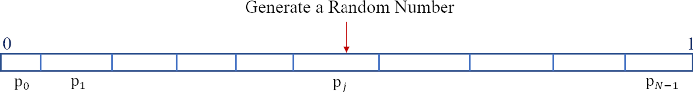
We encode $p_i$ in Eq. (3) using the length of a segment in $[0,1]$
 . All segments are concatenated in order to build the unit interval. The segment index is the cluster index. These segments are called the interval representation as shown in Fig. 4. To draw a sample from subspace $S_2$
 , we use the uniform random number generator to select a random number from interval $[0,1]$
 . This random number indicates the cluster index on the interval representation.
Illustration of the interval representation, where the length of a segment in the unit interval represents the probability of a cluster, $p_i$ . A random number is generated in the unit interval to indicate the cluster index.
To generate a new sample in $S_2$ , we perform the following steps:
(i) Select a random number from the uniform random number generator to determine the cluster index.
(ii) Draw a set of samples independently from the Gaussian distribution.
(iii) Match histograms of the generated Gaussian samples with the inverse CDFs in the chosen cluster.
(iv) Repeat Steps 1–3 if the generated sample of Step 3 has no value larger than a pre-set threshold.
(v) Perform the inverse transform of ICA and the inverse transform of PCA.
(vi) Reshape the 1D vector into a 3D tensor and this tensor is the generated sample in $S_2$
.

The above procedure is named Independent Components Histogram Matching (ICHM). To conclude, there are two main modules in core sample generation: spatial dimension reduction (SDR) and independent components histogram matching as shown in Fig. 2.
D) Coarse-to-fine generation
In this section, we examine generation model $G_{i+1}^i$ , whose role is to generate a sample in $S_i$
 given a sample in $S_{i+1}$
 . Analysis model, $E_i^{i+1}$
 , transforms $S_i$
 to $S_{i+1}$
 through the c/w Saab transform in the forward path. In the reverse path, we perform the inverse c/w Saab transform on generated samples in $S_{i+1}$
 to $S_i$
 . We take generation model $G_2^1$
 as an example to explain the generation process from $S_2$
 and to $S_1$
 . A generated sample in $S_2$
 can be partitioned into $K_1$
 groups as shown in the left part of Fig. 5. Each group of channels is composed of one DC channel and several low-frequency AC channels. The $k$
 th group of channels in $S_2$
 , whose number is denoted by $K_2^{(k)}$
 , is derived from the $k$
 th channel in $S_1$
 . We apply the inverse c/w Saab transform to each group individually. The inverse c/w Saab transform converts the tensor at the same spatial location across $K_2^{(k)}$
 channels (represented by white dots in Fig. 5) in $S_2$
 into a block of size $I_i \times I_i$
 (represented by the white parallelogram in Fig. 5) in $S_1$
 , using the DC and AC components obtained in the fine-to-coarse analysis. After the inverse c/w Saab transform, the Saab coefficients in $S_1$
 form a generated sample in $S_1$
 . The same procedure is repeated between $S_1$
 and $S_0$
 .
.
Illustration of the generation process.

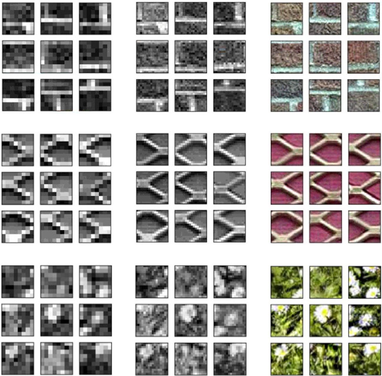
Examples of several generated textures in core $S_2$ , intermediate subspace $S_1$
 , and source $S_0$
 are shown in Fig. 6. The DC channels generated in the core offer gray-scale low-resolution patterns of a generated sample. More local details are added gradually from $S_2$
 to $S_1$
 and from $S_1$
 to $S_0$
 .
.
Examples of generated DC maps in core $S_2$ (first column), generated samples in subspace $S_1$
 (second co-lumn), and the ultimate generated textures in source $S_0$
 (third column).
V. EXPERIMENTS
A) Experimental setup
The following hyper parameters (see Fig. 2) are used in our experiments.
• Input filter window size to Hop-1: $I_0=2$
,• Input filter window size to Hop-2: $I_1=2$
,• Selected channel numbers in Hop-1 ($K_1$
): $6\sim 10$,• Selected channel numbers in Hop-2 ($K_2$
): $20\sim 30$.


The window size of the analysis filter is the same as the generation window size. All windows are non-overlapping with each other. The actual channel numbers $K_1$ and $K_2$
 are texture-dependent. That is, we examine the energy distribution based on the PCA eigenvalues and choose the knee point where the energy becomes flat.
B) An example: brick wall generation
We show generated brick_wall patches of size $32\times 32$ and $64\times 64$
 in Figs 7(a) and 7(c). We performed two-stage c/w Saab transforms on $32\times 32$
 patches and three-stage c/w Saab transforms on $64\times 64$
 patches, whose core subspace dimensions are 1728 and 4032, respectively. Patches in these figures were synthesized by running the TGHop method in 100rounds. Randomness in each round primarily comes from two factors: (1) random cluster selection, and (2) random seed vector generation.
Examples of generated $brick\_wall$ texture patches and stitched images of larger sizes, where the image in the bottom-left corner is the exemplary texture image and the patches highlighted by red squared boxes are unseen patterns. (a) Synthesized $32\times 32$
 patches. (b) Stitched images with $32\times 32$
 patches. (c) Synthesized $64\times 64$
 patches. (d) Stitched images with $64\times 64$
 patches.
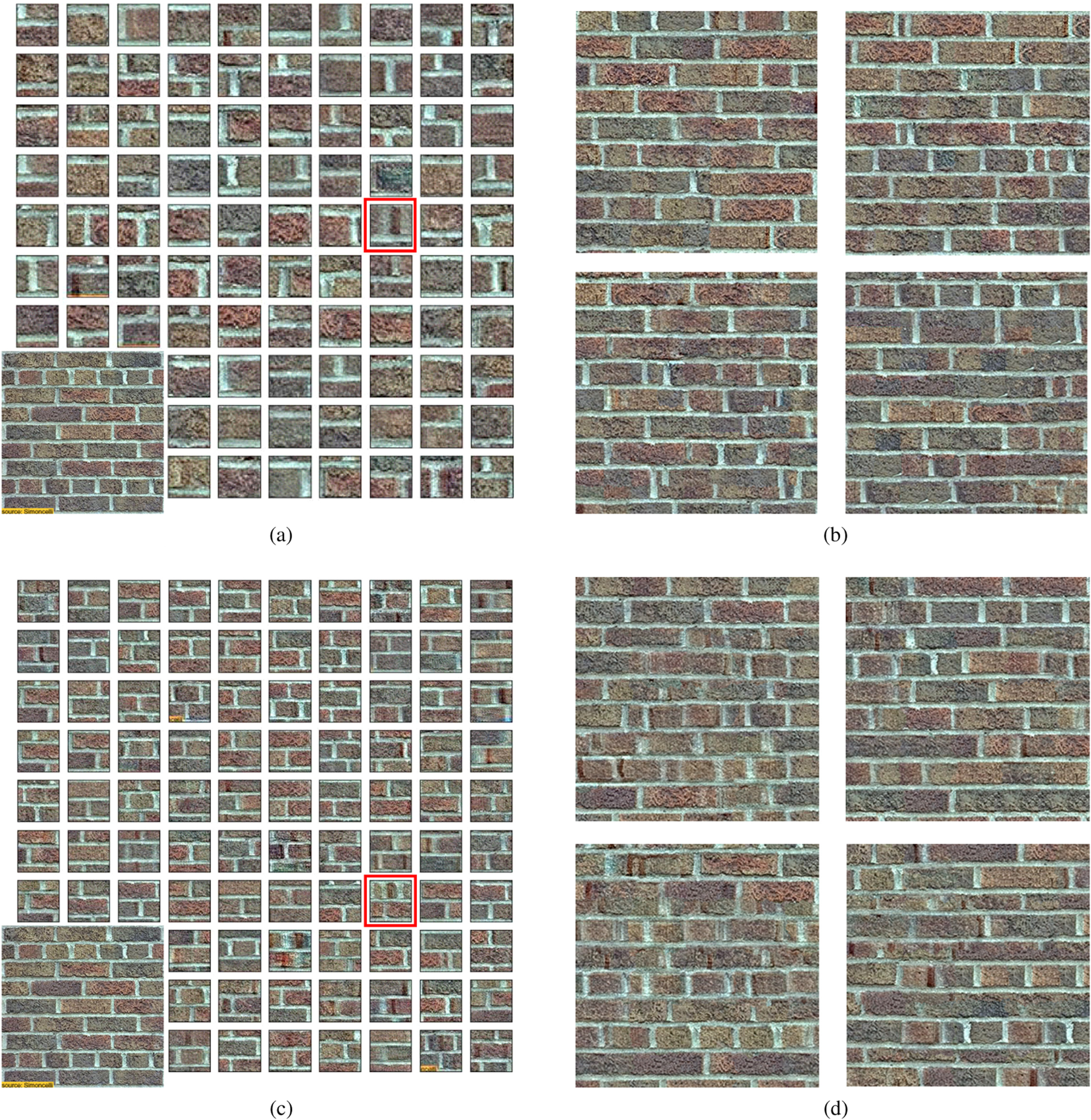
Generated patches retain the basic shape of bricks and the diversity of brick texture. We observe some unseen patterns generated by TGHop, which are highlighted by red squared boxes in Figs 7(a) and 7(c). As compared with generated $32\times 32$ patches, generated $64\times 64$
 patches were sometimes blurry (e.g., the one in the upper right corner) due to a higher source dimension.
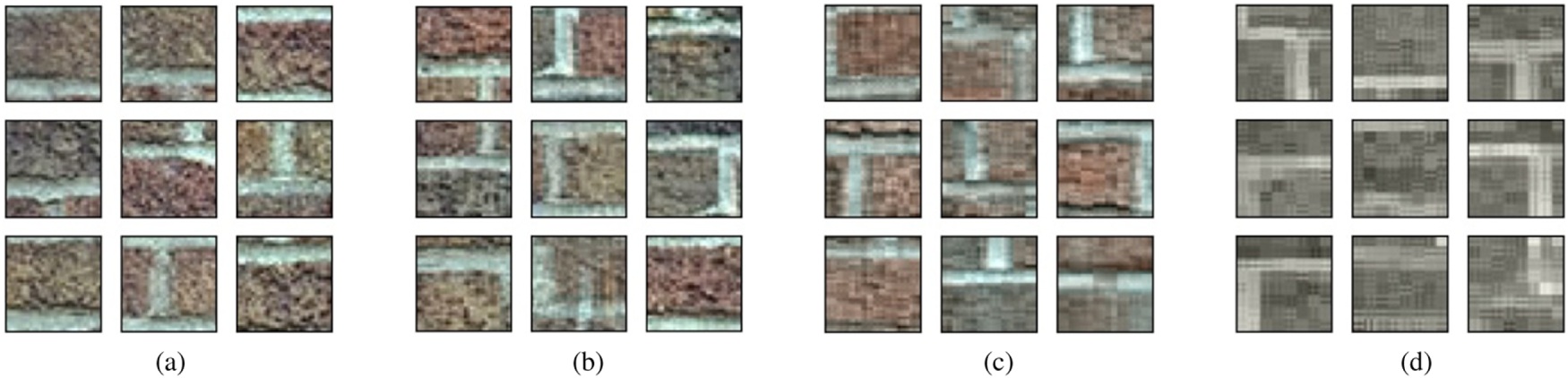
As a non-parametric model, TGHop can choose multiple settings under the same pipeline. For example, it can select different channel numbers in $\tilde {S}_1$ and $\tilde {S}_2$
 to derive different generation results. Four settings are listed in Table 1. The corresponding generation results are shown in Fig. 8. Dimensions decrease faster from (a) to (d). The quality of generated results becomes poorer due to smaller dimensions of the core subspace, $\tilde {S}_2$
 , and the intermediate subspace, $\tilde {S}_1$
 .
.
The settings of four generation models.

Generated patches using different settings, where the numbers below the figure indicates the dimensions of $S_0$ , $S_1$
 , and $S_2$
 , respectively. (a) $3072\rightarrow 2560\rightarrow 2048$
 . (b) $3072\rightarrow 1536\rightarrow 768$
 . (c) $3072\rightarrow 1280\rightarrow 512$
 . (d) $3072\rightarrow 768\rightarrow 192$
 .
.
To generate larger texture images, we first generate 5000 texture patches and perform image quilting [Reference Efros and Freeman13] with them. The results after quilting are shown in Figs 7(b) and 7(d). All eight images are of the same size, i.e., $256\times 256$ . They are obtained using different initial patches in the image quilting process. By comparing the two sets of stitched images, the global structure of the brick wall is better preserved using larger patches (i.e. of size $64 \times 64$
 ) while its local detail is a little bit blurry sometimes.
C) Performance benchmarking with DL-based methods
C.1 Visual quality comparison
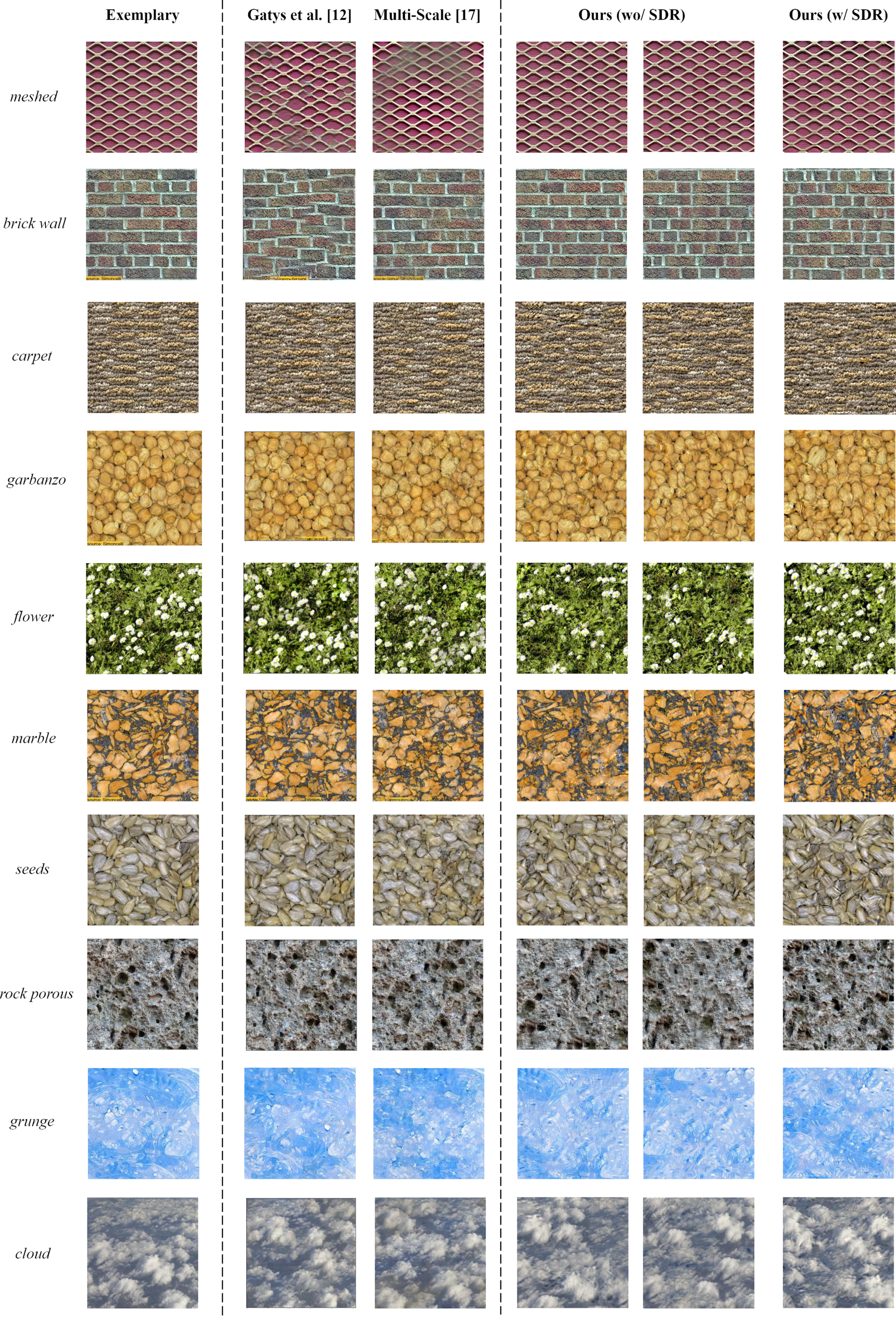
The quality of generated texture is usually evaluated by human eyes. Subjective user study is not a common choice for texture synthesis because different people have different standards to judge the quality of generated texture images. Evaluation metrics such as Inception Score [Reference Salimans, Goodfellow, Zaremba, Cheung, Radford and Chen50] or Fréchet Inception Distance [Reference Heusel, Ramsauer, Unterthiner, Nessler and Hochreiter51] are proposed for natural image generation. These metrics however demand sufficient number of samples to evaluate the distributions of generated images and real images, which are not suitable for texture synthesis containing only one image for reference. The value of loss function was used to measure texture quality or diversity for CNN-based methods [Reference Li, Fang, Yang, Wang, Lu and Yang23, Reference Shi and Qiao26]. A lower loss however does not guarantee better generation quality. Since TGHop dose not have a loss function, we show generated results of two DL-based methods and TGHop side by side in Fig. 9 for 10 input texture images collected from [Reference Portilla and Simoncelli19, Reference Gatys, Ecker and Bethge20, Reference Ustyuzhaninov, Brendel, Gatys and Bethge25] or the Internet. The benchmarking DL methods were proposed by Gatys et al. [Reference Gatys, Ecker and Bethge20] and Ustyuzhaninov et al. [Reference Ustyuzhaninov, Brendel, Gatys and Bethge25]. By running their codes, we show their results in the second and third columns of Fig. 9, respectively, for comparison. These results are obtained by default iteration numbers; namely, 2000 in [Reference Gatys, Ecker and Bethge20] and 4000 in [Reference Gatys, Ecker and Bethge20]. The results of TGHop are shown in the last three columns. The left two columns are obtained without SDR in two different runs while the last column is obtained with SDR. There is little quality degradation after dimension reduction of $S_2$ with SDR. For meshed and cloud textures, the brown fog artifact in [Reference Gatys, Ecker and Bethge20, Reference Ustyuzhaninov, Brendel, Gatys and Bethge25] is apparent. In contrast, it does not exist in TGHop. More generated images using TGHop are given in Fig. 10. As shown in Figs 9 and 10, TGHop can generate high-quality and visually pleasant texture images.
Comparison of texture images generated by two DL-based methods and TGHop (from left to right): exemplary texture images, texture images generated by [Reference Gatys, Ecker and Bethge20], by [Reference Ustyuzhaninov, Brendel, Gatys and Bethge25], two examples by TGHop without spatial dimension reduction (SDR) and one example by TGHop with SDR.
More texture images generated by TGHop.

C.2 Comparison of generation time
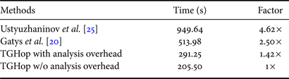
We compare the generation time of different methods in Table 2. All experiments were conducted on the same machine composed of 12 CPUs (Intel Core i7-5930K CPU at 3.50GHz) and 1 GPU (GeForce GTX TITAN X). GPU was needed in two DL-based methods but not in TGHop. We set the iteration number to 1000 for [Reference Gatys, Ecker and Bethge20] and 100 for [Reference Ustyuzhaninov, Brendel, Gatys and Bethge25]. TGHop generated 10K $32\times 32$ patches for texture quilting. For all three methods, we show the time needed in generating one image of size $256\times 256$
 in Table 2, TGHop generates one texture image in 291.25 s while Gatys’ method and Ustyuzhaninov's method demand 513.98 and 949.64 s, respectively. TGHop is significantly faster.
Comparison of time needed to generate one texture image.
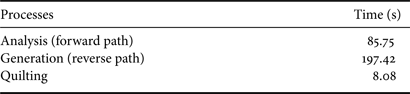
We break down the generation time of TGHop into three parts: (1) successive subspace analysis (i.e. the forward path), (2) core and successive subspace generation (i.e. the reverse path), and (3) the quilting process. The time required for each part is shown in Table 3. They demand 85.75, 197.42, and 8.08 s, respectively. To generate multiple images from the same exemplary texture, we run the first part only once, which will be shared by all generated texture images, and the second and third parts multiple times (i.e. one run for a new image). As a result, we can view the first part as a common overhead and count the last two parts as the time for single texture image generation. This is equal to 205.5 s. The two DL benchmarks do not have such a breakdown and need to go through the whole pipeline to generate one new texture image.
The time of three processes in our method.
D) Comparison of model sizes
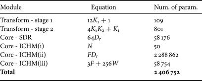
The model size is measured by the number of parameters. The size of TGHop is calculated below.
• Two-stage c/w Saab Transforms
The forward analysis path and the reverse generation path share the same two-stage c/w Saab transforms. For an input RGB patch, the input tensor of size $2\times 2 \times 3=12$
is transformed into a $K_1$-D tensor in the first-stage transform, leading a filter size of $12 K_1$ plus one shared bias. For each of $K_1$ channels, the input tensor of size $2\times 2$ is transformed into a tensor in the second stage transform. The sum of the output dimensions is $K_2$. The total parameter number for all $K_1$ channels is $4 K_1 K_2$ plus $K_1$ biases. Thus, the total number of parameters in the two-stage transforms is $13K_1+4K_1K_2+1$.• Core Sample Generation
Sample generation in the core contains two modules: SDR and ICHM. For the first module, SDR is implemented by $K_2$
PCA transforms, where the input of size $8\times 8=64$ and the output is a $K_{r_i}$ dimensional vector, yielding the size of each PCA transformation matrix to be $64\times K_{r_i}$. The total number of parameters is $64\times \sum _{i=1}^{K_2}{K_{r_i}}=64D_r$, where $D_r$ is the dimension of the concatenated output vector after SDR. For the second module, it has three components:
• Interval representation $p_0,\ldots ,p_{N-1}$
$N$ parameters are needed for $N$ cluster.• Transform matrices of FastICAIf the input vector is of dimension $D_r$
and the output dimension of FastICA is $K_{c_{i}}$ for the $i$th cluster, $i=1, \ldots ,N$, the total parameter number of all transform matrices is $D_r F$, where $F=\sum _{i=1}^{N}{K_{c_i}}$ is the number of CDFs.• Codebook size of quantized CDFsThe codebook contains the index, the maximum and the minimum values for each CDF. Furthermore, we have $W$
clusters of CDF, where all CDFs in each cluster share the same bin structure of 256 bins. As a result, the total parameter number is $3F+256W$.
.


The above equations are summarized and an example is given in Table 4 under the experiment setting of $N=50$ , $K_1=9$
 , $K_2=22$
 , $D_r=909$
 , $F=2518$
 , and $W=200$
 . The model size of TGHop is 2.4M. For comparison, the model sizes of [Reference Gatys, Ecker and Bethge20] and [Reference Ustyuzhaninov, Brendel, Gatys and Bethge25] are 0.852 and 2.055M, respectively. A great majority of TGHop model parameters comes from ICHM(ii). Further model size reduction without sacrificing generated texture quality is an interesting extension of this work.
The number of parameters of TGHop, under the setting of $\gamma =0.01$ , $N=50$ $K_1=9$
 , $K_2=22$
 , $D_r=909$
 , $F=2,518$
 and $W=200$
 .
.
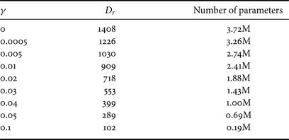
As compared with [Reference Lei, Zhao and Kuo28], SDR is a new module introduced in this work. It helps remove correlations of spatial responses to reduce the model size. We examined the impact of using different threshold $\gamma$ in SDR on texture generation quality and model size with brick_wall texture. The same threshold is adopted for all channels to select PCA components. The dimension of reduced space, $D_r$
 , and the cluster number, $N$
 , are both controlled by threshold $\gamma$
 , used in SDR. $\gamma =0$
 represents all 64 PCA components are kept in SDR. We can vary the value of $\gamma$
 to get a different cluster number and the associated model size. The larger the value of $\gamma$
 , the smaller $D_r$
 and $N$
 and, thus, the smaller the model size as shown in Table 5. The computation given in Table 4 is under the setting of $\gamma =0.01$
 .
.
The reduced dimension, $D_r$ , and the model size as a function of threshold $\gamma$
 used in SDR.
A proper cluster number is important since too many clusters lead to larger model sizes while too few clusters result in bad generation quality. To give an example, consider the brick_wall texture image of size $256\times 256$ , where the dimension of $S_2$
 is $8\times 8 \times 22=1408$
 with $K_2=22$
 . We extract 12 769 patches of size $32\times 32$
 (with stride 2) from this image. We conduct experiments with $N=$
 50, 80, 110, and 200 clusters and show generated patches in Fig. 11. As shown in (a), 50 clusters were too few and we see the artifact of over-saturation in generated patches. By increasing $N$
 from 50 to 80, the artifact still exists but is less apparent in (b). The quality improves furthermore when $N=100$
 as shown in (c). We see little quality improvement when $N$
 goes from 100 to 200. Furthermore, patches generated using different thresholds $\gamma$
 are shown in Fig. 12. We see little quality degradation from (a) to (f) while the dimension is reduced from 1408 to 553. Image blur shows up from (g) to (i), indicating that some details were discarded along with the corresponding PCA components.
Generated brick_wall patches using different cluster numbers in independent component histogram matching. (a) 50 clusters. (b) 80 clusters. (c) 110 clusters. (d) 200 clusters.

Generated brick_wall patches using different threshold $\gamma$ values in SDR. (a) $\gamma =0$
 . (b) $\gamma =0.0005$
 . (c) $\gamma =0.005$
 . (d) $\gamma =0.01$
 . (e) $\gamma =0.02$
 . (f) $\gamma =0.03$
 . (g) $\gamma =0.04$
 . (h) $\gamma =0.05$
 . (i) $\gamma =0.1$
 .
.

VI. CONCLUSION AND FUTURE WORK
An explainable, efficient, and lightweight texture generation method, called TGHop, was proposed in this work. Texture can be effectively analyzed using the multi-stage c/w Saab transforms and expressed in the form of joint spatial-spectral representations. The distribution of sample texture patches was carefully studied so that we can generate samples in the core. Based on generated core samples, we can go through the reverse path to increase its spatial dimension. Finally, patches can be stitched to form texture images of a larger size. It was demonstrated by experimental results that TGHop can generate texture images of superior quality with a small model size and at a fast speed.
Future research can be extended in several directions. Controlling the growth of dimensions of intermediate subspaces in the generation process appears to be important. Is it beneficial to introduce more intermediate subspaces between the source and the core? Can we apply the same model for the generation of other images such as human faces, digits, scenes, and objects? Is it possible to generalize the framework to image inpainting? How does our generation model compare to GANs? These are all open and interesting questions for further investigation.
ACKNOWLEDGEMENTS
This research was supported by a gift grant from Mediatek. Computation for the work was supported by the University of Southern California's Center for High Performance Computing (hpc.usc.edu).
Xuejing Lei received the B.E. degree in Automation from Xi'an Jiaotong University, Xi'an, China, in 2016, and the M.S. degree in Electrical Engineering from the University of Southern California, Los Angeles, USA, in 2018. She is currently pursuing the Ph.D. degree in Electrical and Computer Engineering from the University of Southern California, Los Angeles, USA. Her research interests lie in machine learning and computer vision including video segmentation and tracking, image generative modeling, and 3D object reconstruction.
Ganning Zhao received her B.E. degree in Automation from Guangdong University of Technology, Guangzhou, China, in 2019. She is currently pursuing the Ph.D. degree in Electrical Engineering from the University of Southern California, Los Angeles, USA. Her research interests lie in machine learning and computer vision including image generative modeling and 3D point cloud.
Kaitai Zhang received the B.S. degree in Physics from Fudan University, Shanghai, China, in 2016, and the Ph.D. degree in Electrical and Computer Engineering from the University of Southern California (USC), Los Angeles, USA, in 2021. He was fortunate enough to join the Media Communication Lab at USC and have Prof. C.-C. Jay Kuo as his Ph.D. advisor, and his research interests include image processing, computer vision, and machine learning.
C.-C. Jay Kuo (F’99) received the B.S. degree in Electrical Engineering from the National Taiwan University, Taipei, Taiwan, in 1980, and the M.S. and Ph.D. degrees in Electrical Engineering from the Massachusetts Institute of Technology, Cambridge, in 1985 and 1987, respectively. He is currently the Director of the Multimedia Communications Laboratory and a Distinguished Professor of electrical engineering and computer science at the University of Southern California, Los Angeles. His research interests include digital image/video analysis and modeling, multimedia data compression, communication and networking, and biological signal/image processing. He is a co-author of 310 journal papers, 970 conference papers, 30 patents, and 14 books. Dr. Kuo is a Fellow of the American Association for the Advancement of Science (AAAS) and The International Society for Optical Engineers (SPIE).


 Open access