





1. Introduction
A predictive understanding of turbulent transport in magnetised fusion plasmas relies largely on first-principles gyrokinetic (GK) simulations, whose five-dimensional phase-space resolution is computationally demanding. This computational cost limits, for example, the rapid exploration of the parameter space of fusion devices, ultimately hindering their development. Moment-based formulations of the GK model (Jorge, Ricci & Loureiro Reference Jorge, Ricci and Loureiro2017; Mandell, Dorland & Landreman Reference Mandell, Dorland and Landreman2018; Frei et al. Reference Frei, Jorge and Ricci2020, Reference Frei, Ulbl, Trilaksono and Jenko2025) recast the velocity-space dependence into a hierarchy of coupled Hermite–Laguerre moments, which we refer to as gyromoments (GMs). In practice, simulation and theoretical results show that substantially fewer moments than grid points are often needed for comparable accuracy (Frei, Hoffmann & Ricci Reference Frei, Hoffmann and Ricci2022; Hoffmann et al. Reference Hoffmann, Frei and Ricci2023b ; Frei et al. Reference Frei, Ulbl, Trilaksono and Jenko2025).
The GM hierarchy requires a closure because the evolution equation for each moment is coupled to higher-order moments, a consequence of phase-mixing and finite-Larmor-radius effects (Grant & Feix Reference Grant and Feix1967; Jorge et al. Reference Jorge, Ricci and Loureiro2017). Closure schemes for moment hierarchies have a long history in plasma turbulence research. Earlier closures of gyrofluid models (Hammett & Perkins Reference Hammett and Perkins1990; Dorland & Hammett Reference Dorland and Hammett1993; Snyder, Hammett & Dorland Reference Snyder, Hammett and Dorland1997; Waltz et al. Reference Waltz, Staebler, Dorland, Hammett, Kotschenreuther and Konings1997), despite showing very close agreement with full GK simulations in linear growth rates and Landau damping, often struggled to accurately capture nonlinear turbulence saturation levels and the zonal-flow (ZF) dynamics (Dimits et al. Reference Dimits2000). More recently, a naive truncation closure, i.e. setting all moments above a certain cutoff to zero, showed very good agreement once the number of retained moments was sufficiently large (Frei et al. Reference Frei, Hoffmann, Ricci, Brunner and Tecchioll2023; Hoffmann et al. Reference Hoffmann, Frei and Ricci2023a ). However, when the number of moments retained is comparable to that of gyrofluid models, such a truncation breaks conservation properties, leading to erroneous transport predictions. At the same time, approaches inspired by large-eddy-simulation techniques have been explored in GKs, using truncation and/or selective damping of higher-order moments to reduce computational cost while maintaining physical fidelity (Morel et al. Reference Morel, Navarro, Albrecht-Marc, Carati, Merz, Görler and Jenko2011; Bañón Navarro et al. Reference Bañón Navarro, Teaca, Jenko, Hammett and Happel2014). Despite these advances, an effective and systematically justified closure that preserves nonlinear regulation mechanisms when only a reduced number of GMs is retained to minimise computational cost remains an open issue and motivates the present work.
Asymptotic limits provide one possible route to formulating a closure for the GM model. Applying the hot-electron limit (HEL), that is, considering the ion-to-electron temperature ratio $\tau \ll 1$
, to the local
$\tau \ll 1$
, to the local $\delta f$
GK system (Beer, Cowley & Hammett Reference Beer, Cowley and Hammett1995), with
$\delta f$
GK system (Beer, Cowley & Hammett Reference Beer, Cowley and Hammett1995), with $\mathcal{O}(\tau )$
corrections retained only where needed to preserve leading dynamical couplings, yields a three-field fluid model for density, parallel velocity and parallel temperature, as derived by Ivanov et al. (Reference Ivanov, Schekochihin, Dorland, Field and Parra2020, Reference Ivanov, Schekochihin and Dorland2022). We refer to this model as the Ivanov model, which is shown to successfully reproduce a Dimits shift and ZF features in a Z-pinch geometry (with adiabatic electrons). Despite these promising results in a simplified geometry, to our knowledge, the Ivanov model has not yet been systematically benchmarked against GK simulations, leaving the scope and limits of its validity uncertain. This calls for further investigation of the HEL closure to understand, for instance, whether the Ivanov model appears within the GM hierarchy under the same ordering and whether a GK code can reproduce HEL results using a suitably small
$\mathcal{O}(\tau )$
corrections retained only where needed to preserve leading dynamical couplings, yields a three-field fluid model for density, parallel velocity and parallel temperature, as derived by Ivanov et al. (Reference Ivanov, Schekochihin, Dorland, Field and Parra2020, Reference Ivanov, Schekochihin and Dorland2022). We refer to this model as the Ivanov model, which is shown to successfully reproduce a Dimits shift and ZF features in a Z-pinch geometry (with adiabatic electrons). Despite these promising results in a simplified geometry, to our knowledge, the Ivanov model has not yet been systematically benchmarked against GK simulations, leaving the scope and limits of its validity uncertain. This calls for further investigation of the HEL closure to understand, for instance, whether the Ivanov model appears within the GM hierarchy under the same ordering and whether a GK code can reproduce HEL results using a suitably small $\tau$
parameter. In addition, the application of the closure to tokamak geometry and the comparison with finite-
$\tau$
parameter. In addition, the application of the closure to tokamak geometry and the comparison with finite- $\tau$
GK results remain open issues.
$\tau$
GK results remain open issues.
In this paper, we address these points by deriving the HEL of the GM model through a proper expansion in $\tau$
. A set of fluid equations (density, parallel velocity, parallel temperature and perpendicular temperature) is obtained. We show analytically the equivalence of this model the Ivanov model in a Z-pinch geometry, and we confirm numerically that the GM hierarchy yields a closed four-moment system that reproduces the linear and nonlinear results of the Ivanov model to good accuracy in the small-
$\tau$
. A set of fluid equations (density, parallel velocity, parallel temperature and perpendicular temperature) is obtained. We show analytically the equivalence of this model the Ivanov model in a Z-pinch geometry, and we confirm numerically that the GM hierarchy yields a closed four-moment system that reproduces the linear and nonlinear results of the Ivanov model to good accuracy in the small- $\tau$
regime. In particular, our numerical study benchmarks linear Z-pinch ion temperature gradient (ITG) growth-rate convergence against previous results (Ivanov et al. Reference Ivanov, Schekochihin, Dorland, Field and Parra2020, Reference Ivanov, Schekochihin and Dorland2022). Nonlinear simulations accurately recover heat flux levels and reproduce bursty or blow-up behaviour at low collisionality, capturing the transition where ZF reinforcement weakens, as also shown by Ivanov et al. (Reference Ivanov, Schekochihin, Dorland, Field and Parra2020, Reference Ivanov, Schekochihin and Dorland2022). A detailed analysis of turbulence prediction in the Z-pinch geometry is then presented. Next, we extend the HEL GM model to more complex geometries. Specifically, we focus on the tokamak
$\tau$
regime. In particular, our numerical study benchmarks linear Z-pinch ion temperature gradient (ITG) growth-rate convergence against previous results (Ivanov et al. Reference Ivanov, Schekochihin, Dorland, Field and Parra2020, Reference Ivanov, Schekochihin and Dorland2022). Nonlinear simulations accurately recover heat flux levels and reproduce bursty or blow-up behaviour at low collisionality, capturing the transition where ZF reinforcement weakens, as also shown by Ivanov et al. (Reference Ivanov, Schekochihin, Dorland, Field and Parra2020, Reference Ivanov, Schekochihin and Dorland2022). A detailed analysis of turbulence prediction in the Z-pinch geometry is then presented. Next, we extend the HEL GM model to more complex geometries. Specifically, we focus on the tokamak $s{-}\alpha$
geometry for Cyclone Base Case (CBC) parameters (Lin et al. Reference Lin, Hahm, Lee, Tang and Diamond1999), a standard test case considered by many GK codes (Dimits et al. Reference Dimits2000). The HEL GM model predicts an ITG-like instability and qualitatively accurate heat-flux levels in comparison with GK simulations. This indicates that the HEL closure can be applied outside its formal range of validity. On the other hand, the HEL GM model overpredicts transport when approaching marginal stability. For instance, we do not observe a Dimits shift in the HEL model when considering the tokamak geometry, which indicates that the HEL closure does not overcome the limitations of the lowest-order moment truncation observed in Hoffmann et al. (Reference Hoffmann, Frei and Ricci2023a
). This shortfall indicates that higher-order moments beyond the four retained in the HEL closure play an essential role in sustaining ZF regulation closer to marginal stability. This comparison also highlights the more favourable conditions for ZF activity in a Z-pinch geometry.
$s{-}\alpha$
geometry for Cyclone Base Case (CBC) parameters (Lin et al. Reference Lin, Hahm, Lee, Tang and Diamond1999), a standard test case considered by many GK codes (Dimits et al. Reference Dimits2000). The HEL GM model predicts an ITG-like instability and qualitatively accurate heat-flux levels in comparison with GK simulations. This indicates that the HEL closure can be applied outside its formal range of validity. On the other hand, the HEL GM model overpredicts transport when approaching marginal stability. For instance, we do not observe a Dimits shift in the HEL model when considering the tokamak geometry, which indicates that the HEL closure does not overcome the limitations of the lowest-order moment truncation observed in Hoffmann et al. (Reference Hoffmann, Frei and Ricci2023a
). This shortfall indicates that higher-order moments beyond the four retained in the HEL closure play an essential role in sustaining ZF regulation closer to marginal stability. This comparison also highlights the more favourable conditions for ZF activity in a Z-pinch geometry.
The numerical results presented here are obtained with Gyacomo (Hoffmann et al. Reference Hoffmann, Frei and Ricci2023a
), a numerical simulation code that solves the local $\delta f$
GK equation using the GM approach. The code uses field-aligned coordinates and a Fourier representation in the perpendicular plane, allowing for efficient simulations of plasma turbulence in both Z-pinch and tokamak geometries. The HEL GM model is implemented in Gyacomo by retaining only the four lowest-order moments and scaling the gradients and collisionality according to the HEL ordering.
$\delta f$
GK equation using the GM approach. The code uses field-aligned coordinates and a Fourier representation in the perpendicular plane, allowing for efficient simulations of plasma turbulence in both Z-pinch and tokamak geometries. The HEL GM model is implemented in Gyacomo by retaining only the four lowest-order moments and scaling the gradients and collisionality according to the HEL ordering.
The remainder of this paper is organised as follows. Section 2 presents the GM hierarchy, its HEL closure and its simplification in the Z-pinch geometry. Section 3 reports benchmarks against existing results. Section 4 examines nonlinear Z-pinch turbulence in two and three dimensions. Section 5 extends the application of the HEL closure to the $s$
–
$s$
– $\alpha$
geometry and finite
$\alpha$
geometry and finite $\tau$
. Finally, § 6 summarises our findings and outlines possible extensions of the moment closure.
$\tau$
. Finally, § 6 summarises our findings and outlines possible extensions of the moment closure.
2. Gyrokinetic model
We model ion-scale turbulence in a magnetised plasma using the local, electrostatic, $\delta f$
GK framework with an adiabatic electron response (Catto Reference Catto1978). The model evolves the perturbed ion distribution function
$\delta f$
GK framework with an adiabatic electron response (Catto Reference Catto1978). The model evolves the perturbed ion distribution function $g_i(x,y,z,s_{\parallel },w_{\perp },t)$
in field-aligned coordinates (Beer et al. Reference Beer, Cowley and Hammett1995), where
$g_i(x,y,z,s_{\parallel },w_{\perp },t)$
in field-aligned coordinates (Beer et al. Reference Beer, Cowley and Hammett1995), where $x$
represents the direction perpendicular to the magnetic flux surface,
$x$
represents the direction perpendicular to the magnetic flux surface, $y$
the field-line label,
$y$
the field-line label, $z$
the coordinate aligned with the magnetic field,
$z$
the coordinate aligned with the magnetic field, $s_{\parallel }$
the velocity parallel to the magnetic field,
$s_{\parallel }$
the velocity parallel to the magnetic field, $w_{\perp }$
the magnetic moment and
$w_{\perp }$
the magnetic moment and $t$
the time. The perturbed distribution function satisfies the gyrokinetic equation, which, in normalised units (see table 1), is given by Frei et al. (Reference Frei, Hoffmann and Ricci2022) and Hoffmann et al. (Reference Hoffmann, Frei and Ricci2023a
)
$t$
the time. The perturbed distribution function satisfies the gyrokinetic equation, which, in normalised units (see table 1), is given by Frei et al. (Reference Frei, Hoffmann and Ricci2022) and Hoffmann et al. (Reference Hoffmann, Frei and Ricci2023a
)
 \begin{align} \partial _t g_i & + \{\langle \phi \rangle , g_i\}_{xy} + \sqrt {2\tau } s_\parallel \hat C_\parallel h_i - \frac {\sqrt {2}}{2}\sqrt {\tau } w_\perp \hat C_\parallel \ln B \partial _{s_\parallel } h_i + \frac {\tau }{q_i}(2 s_\parallel ^2+w_\perp ) \hat C_{\perp } h_i \nonumber \\[5pt] & +\left [R_N + \left (s_\parallel ^2+w_\perp -\frac {3}{2}\right ) R_T\right ]\partial _y \langle \phi \rangle = C_{i}. \end{align}
Dimensionless variables used throughout the paper. For a dimensionless variable $A$
, its equivalent in physical units is explicitly denoted as
$A$
, its equivalent in physical units is explicitly denoted as $A^{ph}$
. We introduce the sound velocity
$A^{ph}$
. We introduce the sound velocity $c_{s}=\sqrt {T_{e0}/m_s}$
, the ion thermal velocity
$c_{s}=\sqrt {T_{e0}/m_s}$
, the ion thermal velocity $v_{th i} = \sqrt {T_{i0}/m_i}$
, the magnetic moment
$v_{th i} = \sqrt {T_{i0}/m_i}$
, the magnetic moment $\mu$
, the reference electron temperature
$\mu$
, the reference electron temperature $T_{e0}$
, the reference ion temperature
$T_{e0}$
, the reference ion temperature $T_{i0}$
, the ion thermal Larmor radius
$T_{i0}$
, the ion thermal Larmor radius $\rho _s = c_{s}/\varOmega _i$
, with
$\rho _s = c_{s}/\varOmega _i$
, with $\varOmega _i = q_i^{ph} B_0/m_i$
the ion cyclotron frequency, the reference length scale
$\varOmega _i = q_i^{ph} B_0/m_i$
the ion cyclotron frequency, the reference length scale $R_0$
, the reference magnetic field
$R_0$
, the reference magnetic field $B_0$
, the density and temperature gradient length scales
$B_0$
, the density and temperature gradient length scales $L_N$
and
$L_N$
and $L_T$
, respectively, and the equilibrium Maxwellian distribution function
$L_T$
, respectively, and the equilibrium Maxwellian distribution function $F_{i0}$
.
$F_{i0}$
.

In (2.1), we introduce the gyroaveraged electrostatic potential $\langle \phi \rangle$
, the Jacobian of the field-aligned coordinate system
$\langle \phi \rangle$
, the Jacobian of the field-aligned coordinate system $J_{xyz}$
and the non-adiabatic part of the normalised ion distribution function,
$J_{xyz}$
and the non-adiabatic part of the normalised ion distribution function, $h_i = g_i - \langle \phi \rangle$
. The parameter
$h_i = g_i - \langle \phi \rangle$
. The parameter $\tau = T_i/T_e$
denotes the ion-to-electron temperature ratio, while
$\tau = T_i/T_e$
denotes the ion-to-electron temperature ratio, while $R_N$
and
$R_N$
and $R_T$
represent the density and temperature gradient parameters, respectively. The Poisson bracket
$R_T$
represent the density and temperature gradient parameters, respectively. The Poisson bracket $\{f_1,f_2\}_{xy}=\partial _x f_1 \partial _y f_2 - \partial _y f_1 \partial _x f_2$
arises from the nonlinear
$\{f_1,f_2\}_{xy}=\partial _x f_1 \partial _y f_2 - \partial _y f_1 \partial _x f_2$
arises from the nonlinear $\boldsymbol E\times \boldsymbol B$
drift term, while
$\boldsymbol E\times \boldsymbol B$
drift term, while
 \begin{equation} \hat{C}_{\parallel} = \frac {R_0}{J_{xyz}\hat{B}}\frac {\partial }{\partial z} \end{equation}
denotes the magnetic parallel operator, with $R_0$
being a reference length scale, and where
$R_0$
being a reference length scale, and where
 \begin{equation} \hat C_{\perp}= -\left(\partial_y \ln B + \frac{G_2}{G_1}\partial_z \ln B \right)\frac{\partial}{\partial x} + \left(\partial_x \ln B - \frac{G_3}{G_1}\partial_z \ln B \right)\frac{\partial}{\partial y}\end{equation}
is the magnetic perpendicular operator, where $G_1=g^{xx}g^{yy} - (g^{xy})^2$
,
$G_1=g^{xx}g^{yy} - (g^{xy})^2$
, $G_2=g^{xx}g^{yz} - g^{xy}g^{xz}$
and
$G_2=g^{xx}g^{yz} - g^{xy}g^{xz}$
and $G_3=g^{xy}g^{yz} - g^{yy}g^{xz}$
, and where
$G_3=g^{xy}g^{yz} - g^{yy}g^{xz}$
, and where $g^{ij}=\boldsymbol{\nabla }i \boldsymbol{\cdot }\boldsymbol{\nabla }j$
are the metric coefficients for
$g^{ij}=\boldsymbol{\nabla }i \boldsymbol{\cdot }\boldsymbol{\nabla }j$
are the metric coefficients for $i,j \in \{x,y,z\}$
(D’haeseleer et al. Reference D’haeseleer, Hitchon, Callen and Shohet1991; Beer et al. Reference Beer, Cowley and Hammett1995; Frei et al. Reference Frei, Hoffmann and Ricci2022). The collision term is represented by
$i,j \in \{x,y,z\}$
(D’haeseleer et al. Reference D’haeseleer, Hitchon, Callen and Shohet1991; Beer et al. Reference Beer, Cowley and Hammett1995; Frei et al. Reference Frei, Hoffmann and Ricci2022). The collision term is represented by $C_i$
. The electrostatic potential is determined from the quasi-neutrality condition, assuming an adiabatic electron response
$C_i$
. The electrostatic potential is determined from the quasi-neutrality condition, assuming an adiabatic electron response
 \begin{equation} \left (1 + \frac {q_i}{\tau }\left [ 1 - \varGamma _0 \right ]\right )\phi = q_i n_i + \bar \phi _{yz}, \end{equation}
where $\varGamma _0 = I_0(\rho _i^2\boldsymbol{\nabla} _\perp ^2)e^{-\rho _i^2\boldsymbol{\nabla} _\perp ^2}$
, with
$\varGamma _0 = I_0(\rho _i^2\boldsymbol{\nabla} _\perp ^2)e^{-\rho _i^2\boldsymbol{\nabla} _\perp ^2}$
, with $I_0$
being the modified Bessel function of the first kind,
$I_0$
being the modified Bessel function of the first kind, $\rho _i$
the ion Larmor radius,
$\rho _i$
the ion Larmor radius, $\boldsymbol{\nabla} _\perp$
the perpendicular Laplacian,
$\boldsymbol{\nabla} _\perp$
the perpendicular Laplacian, $n_i$
the ion density fluctuation and
$n_i$
the ion density fluctuation and $\bar \phi _{yz}$
the potential averaged over the
$\bar \phi _{yz}$
the potential averaged over the $y$
and
$y$
and $z$
directions. Details of the GK model can be found in Hoffmann et al. (Reference Hoffmann, Frei and Ricci2023a
).
$z$
directions. Details of the GK model can be found in Hoffmann et al. (Reference Hoffmann, Frei and Ricci2023a
).
2.1. Moment-based approach
To solve the GK Boltzmann equation, we adopt a moment-based approach, projecting the ion GK distribution function onto a basis of Fourier–Hermite–Laguerre modes (Mandell et al. Reference Mandell, Dorland and Landreman2018; Frei et al. Reference Frei, Hoffmann, Ricci, Brunner and Tecchioll2023; Hoffmann et al. Reference Hoffmann, Frei and Ricci2023a ,Reference Hoffmann, Frei and Ricci b ; Mandell et al. Reference Mandell, Dorland, Abel, Gaur, Kim, Martin and Qian2023). We denote these modes as GMs and express them as
 \begin{equation} N_i^{pj}(k_x,k_y,z,t) = \iint \mathrm{d} x \,\mathrm{d} y \iint \mathrm{d}w_{\perp } \,\mathrm{d}s_{\parallel } g_i \,H_p(s_{\parallel })\,L_j(w_{\perp })\, e^{-i(k_x x + k_y y)}, \end{equation}
where $k_x$
is the radial wavenumber,
$k_x$
is the radial wavenumber, $k_y$
the binormal wavenumber,
$k_y$
the binormal wavenumber, $H_p$
the normalised physicist’s Hermite polynomial of order
$H_p$
the normalised physicist’s Hermite polynomial of order $p$
and
$p$
and $L_j$
the Laguerre polynomial of order
$L_j$
the Laguerre polynomial of order $j$
.
$j$
.
In this framework, the gyro-averaging operator can be expressed in terms of Laguerre polynomials as
 \begin{equation} \langle \phi \rangle = \sum _{n=0}^\infty \hat K_n(\ell _\perp )\,L_n(w_{\perp })\phi , \end{equation}
where $\ell _\perp = k_\perp ^2/2$
and
$\ell _\perp = k_\perp ^2/2$
and $k_\perp ^2 = g^{xx}k_x^2 \,+\,2\, g^{xy}k_xk_y \,+\, g^{yy}k_y^2$
. The functions
$k_\perp ^2 = g^{xx}k_x^2 \,+\,2\, g^{xy}k_xk_y \,+\, g^{yy}k_y^2$
. The functions
 \begin{equation} \hat K_n(\ell _\perp ) = \frac {(\tau \ell _\perp )^n}{n!} \, e^{-\tau \ell _\perp } \end{equation}
serve as kernels that separate the configuration- and velocity-space dependencies.
By projecting the local $\delta f$
GK Boltzmann equation onto the Hermite–Laguerre basis, one obtains the following set of GM equations (Hoffmann et al. Reference Hoffmann, Frei and Ricci2023a
):
$\delta f$
GK Boltzmann equation onto the Hermite–Laguerre basis, one obtains the following set of GM equations (Hoffmann et al. Reference Hoffmann, Frei and Ricci2023a
):
 \begin{equation} \partial _t N_i^{pj} + \mathcal S^{pj} + \mathcal M_{\parallel }^{pj} + \mathcal M_{\perp }^{pj} + \mathcal D_{T}^{pj} + \mathcal D_{N}^{pj} = \mathcal C_i^{pj}. \end{equation}
In (2.8), the nonlinear $\boldsymbol E\times \boldsymbol B$
drift term is
$\boldsymbol E\times \boldsymbol B$
drift term is
 \begin{equation} \mathcal S^{pj} = \sum _{n=0}^{\infty }\left \{\hat K_i^n\phi ,\sum _{s=0}^{n+j}d_{njs} N_i^{ps}\right \}_{k_x,k_y}, \end{equation}
where the Poisson bracket in Fourier space, $\left \{\boldsymbol{\cdot },\boldsymbol{\cdot }\right \}_{k_x,k_y}$
, and the Laguerre convolution coefficients,
$\left \{\boldsymbol{\cdot },\boldsymbol{\cdot }\right \}_{k_x,k_y}$
, and the Laguerre convolution coefficients, $d_{njs}$
, such that
$d_{njs}$
, such that $L_nL_j=\sum _{s=0}^{n+j}d_{njs}L_s$
(Gillis & Weiss Reference Gillis and Weiss1960). The trapping and Landau damping term is
$L_nL_j=\sum _{s=0}^{n+j}d_{njs}L_s$
(Gillis & Weiss Reference Gillis and Weiss1960). The trapping and Landau damping term is
 \begin{align} \mathcal M_{\parallel }^{pj} &= \sqrt {\tau } \left \{\hat C_{\parallel }\aleph _i^{p\pm 1,j} - C_\parallel ^B \left [(j+1)\aleph _i^{p\pm 1,j}-j\aleph _i^{p\pm 1,j-1}\right ]\right \}\nonumber \\ &\quad+\sqrt {\tau }C_\parallel ^{B}\sqrt {p}\left[(2j+1)n_i^{p-1,j} -(j+1)n_i^{p-1,j+1} - j n_i^{p-1,j-1}\right ]\!, \end{align}
with $\aleph _i^{p\pm 1,j}=\sqrt {p+1} n_i^{p+1,j} + \sqrt {p} n_i^{p-1,j}$
defined in terms of the non-adiabatic GMs
$\aleph _i^{p\pm 1,j}=\sqrt {p+1} n_i^{p+1,j} + \sqrt {p} n_i^{p-1,j}$
defined in terms of the non-adiabatic GMs
 \begin{equation} n_i^{pj}=N_i^{pj}+q_i/\tau \hat K_i^j\phi \delta _{p0}. \end{equation}
The magnetic centrifugal and perpendicular gradient drift term is
 \begin{align} \mathcal M_{\perp }^{pj} &= \frac {\tau }{q_i} \hat C_{\perp } \left [\sqrt {(p+1)(p+2)} n_i^{p+2,j} + (2p+1)n_i^{pj} + \sqrt {p(p-1)}n_i^{p-2,j}\right ] \end{align}
 \begin{align} &\quad + \frac {\tau }{q_i} \hat C_{\perp } \left [(2j+1)n_i^{pj} - (j+1)n_i^{p,j+1}-jn_i^{p,j-1}\right ], \end{align}
while the diamagnetic temperature and density gradient drift terms are given by
 \begin{equation} \mathcal D_T^{pj} = R_T ik_y\left \{\hat K_i^j\left [\frac {1}{\sqrt {2}}\delta _{p2} -\delta _{p0}\right ]+ \left [(2j+1)\hat K_i^j-(j+1)\hat K_i^{j+1}-j\hat K_i^{j-1}\right ]\delta _{p0}\right \}\phi , \end{equation}
and
 \begin{equation} \mathcal D_N^{pj} = R_N ik_y \hat K_a^j \phi \delta _{p0}, \end{equation}
respectively. Finally, $\mathcal C_i^{pj}$
denotes the projection of the ion–ion collision term.
$\mathcal C_i^{pj}$
denotes the projection of the ion–ion collision term.
When considering an adiabatic electron response, the GM equations are closed by the quasi-neutrality relation
 \begin{equation} \Bigg [1 + \frac {q_i^2}{\tau }\bigg (1-\!\!\sum _{n=0}^{\infty }\hat K_n^2\bigg )\Bigg ]\,\phi - \bar \phi _{yz} = q_i\,\sum _{n=0}^{\infty }\hat K_n\, N_i^{0n}, \end{equation}
where the relation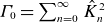 $\varGamma _0 = \sum _{n=0}^{\infty }\hat K_n^2$
is used (Frei, Jorge & Ricci Reference Frei, Jorge and Ricci2020).
$\varGamma _0 = \sum _{n=0}^{\infty }\hat K_n^2$
is used (Frei, Jorge & Ricci Reference Frei, Jorge and Ricci2020).
We refer to the system of (2.8) and (2.16) as the GM model. It describes the evolution of the GMs, $N_i^{pj}$
, and is equivalent to the local GK model in the limit of an infinite number of GMs being retained (
$N_i^{pj}$
, and is equivalent to the local GK model in the limit of an infinite number of GMs being retained ( $p,j\to \infty$
).
$p,j\to \infty$
).
To solve the GM system, we use the Gyacomo codeFootnote
1
(Hoffmann et al. Reference Hoffmann, Frei and Ricci2023a
,Reference Hoffmann, Frei and Ricci
b
, Reference Hoffmann, Balestri and Ricci2025), which uses a Fourier approach for the spatial directions and a fourth-order explicit Runge–Kutta scheme for time integration. The nonlinear term is treated with a $2/3$
-dealiasing method (Orszag Reference Orszag1971). The evolved Fourier modes have perpendicular wavenumbers
$2/3$
-dealiasing method (Orszag Reference Orszag1971). The evolved Fourier modes have perpendicular wavenumbers $k_x = 2\pi m N_x/L_x$
and
$k_x = 2\pi m N_x/L_x$
and $k_y = 2\pi n N_y/L_y$
, for
$k_y = 2\pi n N_y/L_y$
, for $m = -N_x/2+1,\ldots ,N_x/2$
, and
$m = -N_x/2+1,\ldots ,N_x/2$
, and $n = 1\ldots ,N_y/2$
, where
$n = 1\ldots ,N_y/2$
, where $N_x$
and
$N_x$
and $N_y$
represent the radial and binormal resolutions, and
$N_y$
represent the radial and binormal resolutions, and $L_x$
and
$L_x$
and $L_y$
are the radial and binormal box lengths, respectively. A hyperdiffusion damping term of the form
$L_y$
are the radial and binormal box lengths, respectively. A hyperdiffusion damping term of the form $\mu _{hd} (k_\perp /k_{\perp ,max})^4 N_i^{pj}$
, where
$\mu _{hd} (k_\perp /k_{\perp ,max})^4 N_i^{pj}$
, where $\mu _{hd}$
is the hyperdiffusion parameter and
$\mu _{hd}$
is the hyperdiffusion parameter and $k_{\perp ,max}$
is the maximum perpendicular wavenumber in the simulation, is added in the perpendicular direction to dissipate high-frequency modes, as is often done in nonlinear simulations (Jenko, Dorland & Kotschenreuther Reference Jenko, Dorland and Kotschenreuther2000; Hoffmann et al. Reference Hoffmann, Frei and Ricci2023b
). Derivatives along the parallel direction, which has length
$k_{\perp ,max}$
is the maximum perpendicular wavenumber in the simulation, is added in the perpendicular direction to dissipate high-frequency modes, as is often done in nonlinear simulations (Jenko, Dorland & Kotschenreuther Reference Jenko, Dorland and Kotschenreuther2000; Hoffmann et al. Reference Hoffmann, Frei and Ricci2023b
). Derivatives along the parallel direction, which has length $L_z$
, are discretised using a second-order finite-difference scheme on a uniform grid with resolution
$L_z$
, are discretised using a second-order finite-difference scheme on a uniform grid with resolution $N_z$
. Gyacomo supports both tokamak and Z-pinch geometries: in the tokamak geometry, twist-and-shift periodic parallel boundary conditions are applied (Beer et al. Reference Beer, Cowley and Hammett1995), while in the Z-pinch geometry, standard periodic parallel boundary conditions are used (Hoffmann et al. Reference Hoffmann, Frei and Ricci2023b
). For the tokamak geometry, the flux tube length is given by
$N_z$
. Gyacomo supports both tokamak and Z-pinch geometries: in the tokamak geometry, twist-and-shift periodic parallel boundary conditions are applied (Beer et al. Reference Beer, Cowley and Hammett1995), while in the Z-pinch geometry, standard periodic parallel boundary conditions are used (Hoffmann et al. Reference Hoffmann, Frei and Ricci2023b
). For the tokamak geometry, the flux tube length is given by $L_z = 2\pi N_{pol} R_0$
, where
$L_z = 2\pi N_{pol} R_0$
, where $R_0$
is the magnetic axis radius and
$R_0$
is the magnetic axis radius and $N_{pol}$
is the number of poloidal turns. In the Z-pinch geometry,
$N_{pol}$
is the number of poloidal turns. In the Z-pinch geometry, $L_z = 2\pi L_B$
, with
$L_z = 2\pi L_B$
, with $L_B$
as the reference magnetic field length scale, corresponding to the major radius in the tokamak geometry or the pinch radius in the Z-pinch geometry. For the purpose of comparing the two geometries, we set
$L_B$
as the reference magnetic field length scale, corresponding to the major radius in the tokamak geometry or the pinch radius in the Z-pinch geometry. For the purpose of comparing the two geometries, we set $R_0 = L_B$
so that
$R_0 = L_B$
so that $N_{pol}$
can be interpreted as the number of times the field line wraps around the Z-pinch axis. In previous publications (Hoffmann et al. Reference Hoffmann, Frei and Ricci2023a
,
Reference Hoffmann, Frei and Riccib
, Reference Hoffmann, Balestri and Ricci2025), the Gyacomo code evolves the GM model using a truncation closure, setting all GMs with
$N_{pol}$
can be interpreted as the number of times the field line wraps around the Z-pinch axis. In previous publications (Hoffmann et al. Reference Hoffmann, Frei and Ricci2023a
,
Reference Hoffmann, Frei and Riccib
, Reference Hoffmann, Balestri and Ricci2025), the Gyacomo code evolves the GM model using a truncation closure, setting all GMs with $(p,j)\gt (p_{\max },j_{\max })$
, where
$(p,j)\gt (p_{\max },j_{\max })$
, where $p_{\max }$
and
$p_{\max }$
and $j_{\max }$
are the maximum degrees considered for the Hermite–Laguerre basis. In this work, we use a single maximal-degree truncation closure, i.e. we set all GMs with
$j_{\max }$
are the maximum degrees considered for the Hermite–Laguerre basis. In this work, we use a single maximal-degree truncation closure, i.e. we set all GMs with $p+2j \gt d_{\max }$
to vanish, where
$p+2j \gt d_{\max }$
to vanish, where $d_{\max }$
is the maximum moment degree considered. This truncation reflects the structure of fluid models, where the moments are evolved up to a certain velocity-polynomial degree, e.g.
$d_{\max }$
is the maximum moment degree considered. This truncation reflects the structure of fluid models, where the moments are evolved up to a certain velocity-polynomial degree, e.g. $d_{\max }=2$
for a Braginskii-type model (Braginskii Reference Braginskii1965).
$d_{\max }=2$
for a Braginskii-type model (Braginskii Reference Braginskii1965).
2.2. Hot-electron closure
In this subsection, we consider the GM hierarchy up to order $d_{\max }=2$
. This corresponds to evolving the four GMs
$d_{\max }=2$
. This corresponds to evolving the four GMs $N_i^{00}$
,
$N_i^{00}$
, $N_i^{10}$
,
$N_i^{10}$
, $N_i^{20}$
and
$N_i^{20}$
and $N_i^{01}$
in the limit
$N_i^{01}$
in the limit $\tau \ll 1$
for a single-charge ion species (
$\tau \ll 1$
for a single-charge ion species ( $q_i=1$
). In the following, we first write our equations conserving all terms up to a certain power of
$q_i=1$
). In the following, we first write our equations conserving all terms up to a certain power of $\tau$
, without assessing whether these terms are dominant or negligible. The ordering of the different terms will be discussed in the next subsection, where the equivalence with the Ivanov model is established. We expand the kernel functions
$\tau$
, without assessing whether these terms are dominant or negligible. The ordering of the different terms will be discussed in the next subsection, where the equivalence with the Ivanov model is established. We expand the kernel functions $\hat K_n$
, (2.7), for small
$\hat K_n$
, (2.7), for small $\tau$
, namely,
$\tau$
, namely,
 \begin{align} \hat K_0 &= 1 - \ell _\perp \,\tau + \frac 12\,\ell _\perp ^2\,\tau ^2 + \mathcal O(\tau ^3), \end{align}
 \begin{align} \hat K_1 &= \ell _\perp \,\tau - \ell _\perp ^2\,\tau ^2 + \mathcal O(\tau ^3), \end{align}
 \begin{align} \hat K_2 &= \frac 12\,\ell _\perp ^2\,\tau ^2 + \mathcal O(\tau ^3). \end{align}
The non-adiabatic parts of the ion GMs, (2.11), can be written for $(p,j)=(0,0),\,(0,1),\,(0,2)$
as
$(p,j)=(0,0),\,(0,1),\,(0,2)$
as
 \begin{align} n_i^{00} &= N_i^{00} + \Bigl (\tau ^{-1}-\ell _\perp + \frac 12\,\ell _\perp ^2\,\tau \Bigr )\,\phi + \mathcal O(\tau ^2), \end{align}
 \begin{align} n_i^{01} &= N_i^{01} + \bigl (\ell _\perp - \ell _\perp ^2\,\tau \bigr )\,\phi + \mathcal O(\tau ^2), \end{align}
 \begin{align} n_i^{02} &= N_i^{02} + \frac 12\,\ell _\perp ^2\,\tau \,\phi + \mathcal O(\tau ^2), \end{align}
while $n_i^{p,j} = N_i^{p,j} + \mathcal O(\tau ^2)$
for all
$n_i^{p,j} = N_i^{p,j} + \mathcal O(\tau ^2)$
for all $p\gt 0$
and
$p\gt 0$
and $j\gt 2$
. We note that one may be concerned that the expansion of
$j\gt 2$
. We note that one may be concerned that the expansion of $n_i^{00}$
has a
$n_i^{00}$
has a $\tau ^{-1}$
term, which would imply that
$\tau ^{-1}$
term, which would imply that $n_i^{00}$
scales as
$n_i^{00}$
scales as $\mathcal{O}(\tau ^{-1})$
. However, this will be cancelled out by the renormalisation of
$\mathcal{O}(\tau ^{-1})$
. However, this will be cancelled out by the renormalisation of $\phi$
when the equivalence with the Ivanov model is established in the next subsection.
$\phi$
when the equivalence with the Ivanov model is established in the next subsection.
Next, we identify the low-order GMs as pseudo-fluid moments
 \begin{align} n^*=N_i^{00},\quad u_{\parallel }^*=N_i^{10},\quad T_{\parallel }^*=N_i^{20},\quad T_{\perp }^*=N_i^{01},\quad q_\parallel ^*=N_i^{30},\quad q_\perp ^*=N_i^{11}, \end{align}
and
 \begin{align} P_\parallel ^{\parallel *}=N_i^{40},\quad P_\parallel ^{\perp *}=N_i^{21},\quad P_\perp ^{\perp *}=N_i^{02}. \end{align}
These differ slightly from standard fluid moments because the Hermite–Laguerre basis does not match the usual polynomial basis used to evaluate the velocity moments. We assume that all the pseudo-fluid moments scale comparably,
 \begin{align} n^*\sim u_{\parallel }^* \sim T_{\parallel }^* \sim T_{\perp }^* \sim q_\parallel ^* \sim q_\perp ^* \sim P_\parallel ^{\parallel *} \sim P_\parallel ^{\perp *} \sim P_\perp ^{\perp *} \sim \mathcal{O}(1). \end{align}
We now substitute these expansions into the GM hierarchy, (2.8), considering contributions up to $\mathcal O(\tau ^2)$
. This yields a system of equations composed of the density equation,
$\mathcal O(\tau ^2)$
. This yields a system of equations composed of the density equation, $(p,j)=(0,0)$
,
$(p,j)=(0,0)$
,
 \begin{align} \partial _t n^* + \left \{\phi ,n^*\right \} + \tau \,\left \{\ell _\perp \,\phi ,\,T_{\perp }^*-n^*\right \} + \sqrt {\tau }\,\bigl (\hat C_{\parallel } - C_\parallel ^B\bigr )\,u_{\parallel }^* \nonumber \\[6pt] + \tau \,\hat C_{\perp }\,\bigl (\sqrt {2}\,T_{\parallel }^* + 2\,n^* - T_{\perp }^*\bigr ) + \bigl (2\,\hat C_{\perp } + R_N\,i\,k_y\bigr )\,\phi \nonumber \\[-3pt] - \tau [3\hat{C}_{\perp } + (R_N+R_T)ik_y]\ell _\perp \,\phi = \mathcal C_i^{00} + \mathcal O(\tau ^2), \end{align}
the parallel velocity equation, $(p,j)=(1,0)$
,
$(p,j)=(1,0)$
,
 \begin{align} \partial _t u_{\parallel }^* + \left \{\phi ,u_{\parallel }^*\right \} + \tau \,\left \{\ell _\perp \,\phi ,\,q_\perp ^* - u_{\parallel }^*\right \} + \sqrt {\tau }\,\Bigl [\bigl (\hat C_{\parallel } - C_\parallel ^B\bigr )\sqrt {2}\,T_{\parallel }^* + \hat C_{\parallel }\,n^* \nonumber \\[-3pt] - C_\parallel ^B\,T_{\perp }^*\Bigr ] + \frac {1}{\sqrt \tau }\,\hat C_{\parallel }\,\phi - \sqrt \tau \,(\hat C_{\parallel }+C_\parallel ^B)\,\ell _\perp \,\phi + \tau \,\hat C_{\perp }\,\bigl (\sqrt 6\,q_\parallel ^* + 4\,u_{\parallel }^* - q_\perp ^*\bigr ) \nonumber \\[-3pt] = \mathcal C_i^{10} + \mathcal O\left (\tau ^{2}\right )\!, \end{align}
the parallel temperature equation, $(p,j)=(2,0)$
,
$(p,j)=(2,0)$
,
 \begin{align} \partial _t T_{\parallel }^* + \left \{\phi ,T_{\parallel }^*\right \} + \tau \,\left \{\ell _\perp \,\phi ,\,P_\parallel ^{\perp *}-T_{\parallel }^*\right \} + \sqrt {\tau }\,\Bigl [\sqrt {3}\,\bigl (\hat C_{\parallel } - C_\parallel ^B\bigr )\,q_\parallel ^* + \sqrt 2\,\hat C_{\parallel }\,u_{\parallel }^*\Bigr ] \nonumber \\[-3pt] + \tau \,\hat C_{\perp }\,\Bigl (\sqrt {12}\,P_\parallel ^{\parallel *}+6\,T_{\parallel }^* + \sqrt {2}\,n^*\,-\,P_{\parallel }^{\perp *}\Bigr ) + (1-\tau \,\ell _\perp)\bigg(\sqrt 2\,\hat C_{\perp } + \frac {\sqrt 2}{2}\,R_T\,i\,k_y\bigg )\,\phi \nonumber \\[-3pt] = \mathcal C_i^{20} + \mathcal O(\tau ^2),\nonumber \\& \end{align}
and the perpendicular temperature equation, $(p,j)=(0,1)$
,
$(p,j)=(0,1)$
,
 \begin{align} \partial _t T_{\perp }^* + \left \{\phi ,T_{\perp }^*\right \} + \tau \,\left \{\ell _\perp \,\phi ,\,n^* - 2\,T_{\perp }^* + 2\,P_\perp ^{\perp *}\right \} + \sqrt {\tau }\,\hat C_{\parallel }\,q_\perp ^* \nonumber \\[-3pt] + \sqrt {\tau }\,C_\parallel ^B\,u_{\parallel }^* + \tau \,\hat C_{\perp }\,\bigl (\sqrt 2\,P_\parallel ^{\perp *} + 4\,T_{\perp }^* - n^* - 2\,P_\perp ^{\perp *}\bigr ) \nonumber \\[-3pt] - (\hat C_{\perp } + R_T\,i\,k_y)\,\phi + \tau \big[5\,\hat C_{\perp } + (R_T+3\,R_N)\,i\,k_y\big]\,\ell _\perp \,\phi = \mathcal C_i^{01} + \mathcal O(\tau ^2). \end{align}
In addition, assuming adiabatic electrons, the GK quasi-neutrality equation reduces to
 \begin{equation} \big[1 - 2\,\big(\ell _\perp - \tau \,\ell _\perp ^2\big )\big]\,\phi - \langle \phi \rangle _{y z} = n^* + \tau \,\ell _\perp \,\bigl (T_{\perp }^* - n^*\bigr ) + \mathcal O(\tau ^2). \end{equation}
Equations (2.26)–(2.29), together with (2.30), contain higher-order GMs (such as $q_\parallel ^*$
,
$q_\parallel ^*$
, $q_\perp ^*$
, etc.), thus requiring additional assumptions for closure. To close the system, we adopt a mixed-order truncation strategy: we retain
$q_\perp ^*$
, etc.), thus requiring additional assumptions for closure. To close the system, we adopt a mixed-order truncation strategy: we retain $\mathcal O(\tau )$
terms in the density equation while dropping
$\mathcal O(\tau )$
terms in the density equation while dropping $\mathcal O(\tau )$
terms in the higher-order moment equations (parallel velocity, parallel and perpendicular temperatures). Specifically, by dropping
$\mathcal O(\tau )$
terms in the higher-order moment equations (parallel velocity, parallel and perpendicular temperatures). Specifically, by dropping $\mathcal O(\tau )$
terms in the parallel velocity, parallel temperature and perpendicular temperature equations, we obtain
$\mathcal O(\tau )$
terms in the parallel velocity, parallel temperature and perpendicular temperature equations, we obtain
 \begin{align} & \partial _t u_{\parallel }^* + \left \{\phi ,u_{\parallel }^*\right \} + \sqrt {\tau }\,\Bigl [\bigl (\hat C_{\parallel } - C_\parallel ^B\bigr )\sqrt 2\,T_{\parallel }^* + \hat C_{\parallel }\,n^* - C_\parallel ^B\,T_{\perp }^*\Bigr ]\nonumber \\ &\qquad + \frac {1}{\sqrt \tau }\,\hat C_{\parallel }\,\phi - \sqrt \tau \,(\hat C_{\parallel } + C_\parallel ^B)\,\ell _\perp \,\phi = \mathcal{C}_i^{10} + \mathcal O\left (\tau \right )\!, \end{align}
 \begin{align} & \partial _t T_{\parallel }^* + \left \{\phi ,T_{\parallel }^*\right \} + \bigg (\sqrt 2\,\hat C_{\perp } + \frac {\sqrt 2}{2}\,R_T\,i\,k_y \bigg)\,\phi = \mathcal C_i^{20} + \mathcal O(\tau ^{1/2}), \end{align}
 \begin{align} & \partial _t T_{\perp }^* + \left \{\phi ,T_{\perp }^*\right \} - \bigl (\hat C_{\perp } + R_T\,i\,k_y\bigr )\,\phi = \mathcal C_i^{01} + \mathcal O(\tau ^{1/2}). \end{align}
To account for collisions, we consider the gyro-averaged Dougherty operator projected over the Hermite–Laguerre basis (Dougherty Reference Dougherty1964; Frei et al. Reference Frei, Hoffmann and Ricci2022). In the HEL, the collision operator terms are given by
 \begin{align} \mathcal C_i^{00} &= -\,\nu \,\frac {2}{3}\,\tau \,\ell _\perp \,\Bigl (\sqrt 2\,T_{\parallel }^* + T_{\perp }^* + 5\,\ell _\perp \,\phi \Bigr ) + \mathcal O(\tau ^2), \end{align}
 \begin{align} \mathcal C_i^{10} &= \nu \,\mathcal O\left (\tau \right )\!, \end{align}
 \begin{align} \mathcal C_i^{20} &= -\,\nu \,\frac {2}{3}\,\Bigl (2\,T_{\parallel }^* + \sqrt 2\,T_{\perp }^* + 2\sqrt 2\,\ell _\perp \,\phi \Bigr ) + \mathcal O\left (\tau \right )\!, \end{align}
 \begin{align} \mathcal C_i^{01} &= -\,\nu \,\frac {2}{3}\,\Bigl (\sqrt 2\,T_{\parallel }^* + T_{\perp }^* + 2\,\ell _\perp \,\phi \Bigr ) + \mathcal O\left (\tau \right )\!, \end{align}
where $\nu$
is the normalised ion–ion collision frequency. Note that the Landau-based collision operator used in Ivanov et al. (Reference Ivanov, Schekochihin, Dorland, Field and Parra2020) differs from the Dougherty model used here. As a consequence, one should expect slight differences in the small-
$\nu$
is the normalised ion–ion collision frequency. Note that the Landau-based collision operator used in Ivanov et al. (Reference Ivanov, Schekochihin, Dorland, Field and Parra2020) differs from the Dougherty model used here. As a consequence, one should expect slight differences in the small- $\tau$
limit. In the following, we refer to (2.26), (2.31)–(2.33), along with the quasi neutrality condition (2.30), as the HEL–GM model.
$\tau$
limit. In the following, we refer to (2.26), (2.31)–(2.33), along with the quasi neutrality condition (2.30), as the HEL–GM model.
The mixed-order closure employed in the HEL–GM model is an ad hoc truncation strategy designed to demonstrate that the Ivanov model emerges naturally from the GM hierarchy when appropriate limits are taken. This approach allows us to establish that the Ivanov fluid model is embedded within the more general GM hierarchy, thereby demonstrating that appropriate closure choices can recover existing reduced models while retaining the flexibility to extend beyond their original scope of validity.
2.3. Analytical equivalence with the Ivanov model in Z-pinch geometry
We now illustrate that the HEL–GM model recovers the Ivanov model when considering the Z-pinch magnetic geometry ( $R_N=0$
,
$R_N=0$
, $\hat C_{\perp }=-\,i\,k_y$
,
$\hat C_{\perp }=-\,i\,k_y$
, $\hat C_{\parallel }=1$
,
$\hat C_{\parallel }=1$
, $C_\parallel ^B=0$
). Since the Ivanov model does not express the gyroaveraging operator in terms of Bessel functions, we directly expand the gyroaveraged distribution function
$C_\parallel ^B=0$
). Since the Ivanov model does not express the gyroaveraging operator in terms of Bessel functions, we directly expand the gyroaveraged distribution function $g_i(\boldsymbol R)$
(in gyrocentre coordinates
$g_i(\boldsymbol R)$
(in gyrocentre coordinates $\boldsymbol R$
) for small
$\boldsymbol R$
) for small $\tau$
in terms of the distribution function in particle coordinates
$\tau$
in terms of the distribution function in particle coordinates $f_i(\boldsymbol x)$
 \begin{align} g_i(\boldsymbol R) &= \Bigl \langle \,f_i(\boldsymbol x) - \boldsymbol \rho \boldsymbol{\cdot }\boldsymbol{\nabla }\,f_i(\boldsymbol x) + \frac 12\,\boldsymbol \rho \,\boldsymbol \rho : \boldsymbol{\nabla }\boldsymbol{\nabla }\,f_i(\boldsymbol x)\Bigr \rangle + \mathcal O(\tau ^2)\nonumber \\ &= g_i(\boldsymbol x) + \frac {\tau }{2}\,w_{\perp }\,\boldsymbol{\nabla} _\perp ^2\,g_i(\boldsymbol x) + \mathcal O(\tau ^2), \end{align}
where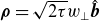 $\boldsymbol \rho = \sqrt {2\tau }w_{\perp }\hat {\boldsymbol b}$
is the gyrocentre displacement vector, with
$\boldsymbol \rho = \sqrt {2\tau }w_{\perp }\hat {\boldsymbol b}$
is the gyrocentre displacement vector, with $\hat {\boldsymbol b}$
the unit vector along the magnetic field and
$\hat {\boldsymbol b}$
the unit vector along the magnetic field and $\boldsymbol{\nabla} _\perp ^2$
, the perpendicular Laplacian operator. Recalling that the gyro-averaging operator,
$\boldsymbol{\nabla} _\perp ^2$
, the perpendicular Laplacian operator. Recalling that the gyro-averaging operator, $\langle \,\boldsymbol{\cdot }\,\rangle$
, satisfies
$\langle \,\boldsymbol{\cdot }\,\rangle$
, satisfies $\langle \boldsymbol \rho \rangle =0$
and
$\langle \boldsymbol \rho \rangle =0$
and $\langle \boldsymbol \rho \,\boldsymbol \rho \rangle = \tau \,w_{\perp }\,\mathbf{I}_\perp$
, with
$\langle \boldsymbol \rho \,\boldsymbol \rho \rangle = \tau \,w_{\perp }\,\mathbf{I}_\perp$
, with $\mathbf{I}_\perp$
the perpendicular projection operator, a pseudo-fluid moment, e.g.
$\mathbf{I}_\perp$
the perpendicular projection operator, a pseudo-fluid moment, e.g. $n^*$
, can be expressed in the particle coordinate system via
$n^*$
, can be expressed in the particle coordinate system via
 \begin{align} n^*(\boldsymbol R) &= \iint \Bigl [g_i(\boldsymbol x) + \frac {\tau }{2}\,w_{\perp }\,\boldsymbol{\nabla} _\perp ^2\,g_i(\boldsymbol x)\Bigr ] \,\mathrm{d}w_{\perp }\,\mathrm{d}s_{\parallel } + \mathcal O(\tau ^2) \nonumber \\ &=n^*(\boldsymbol x) + \frac {\tau }{2}\,\boldsymbol{\nabla} _\perp ^2\bigl (n^* - T_\perp ^*\bigr )(\boldsymbol x) + \mathcal O(\tau ^2), \end{align}
where we assume commutation between the velocity-space integration and the perpendicular Laplacian operator. This assumption is valid in the local approximation, where the perpendicular gradients are considered constant over a Larmor radius. The gyrocentre-to-particle coordinate transformation does not affect the higher-order GMs, as the HEL–GM scaling neglects the $\mathcal O(\tau )$
terms in the parallel velocity, parallel temperature and perpendicular temperature equations.
$\mathcal O(\tau )$
terms in the parallel velocity, parallel temperature and perpendicular temperature equations.
The Ivanov model is then obtained by rewriting the HEL–GM model, (2.26) and (2.31)–(2.33), for the following fluid moments:
 \begin{equation} n(\boldsymbol x) = n^*(\boldsymbol x), \quad u_\parallel (\boldsymbol x) = \frac {\sqrt 2}{2}\,u_{\parallel }^*(\boldsymbol x), \quad T(\boldsymbol x) = \frac {1}{2} \big[\sqrt {2} T_{\parallel }^*(\boldsymbol x) - T_{\perp }^*(\boldsymbol x)\big] - n^*(\boldsymbol x), \end{equation}
and considering a Z-pinch geometry $(\hat C_{\perp }=-\,i\,k_y,\,\hat C_{\parallel }=1,\,C_\parallel ^B=0)$
and
$(\hat C_{\perp }=-\,i\,k_y,\,\hat C_{\parallel }=1,\,C_\parallel ^B=0)$
and $\ell _\perp =\boldsymbol{\nabla} _\perp ^2/2$
. To obtain analytical equivalence with the Ivanov model, it is necessary to rescale the variables with the asymptotically small parameter
$\ell _\perp =\boldsymbol{\nabla} _\perp ^2/2$
. To obtain analytical equivalence with the Ivanov model, it is necessary to rescale the variables with the asymptotically small parameter $\tau$
. Consequently, this procedure modifies the orderings between the evolved moments, which is justified considering the high-collisionality, long-wavelength and large aspect ratio limits used in the Ivanov model. Specifically, the rescaling is defined as
$\tau$
. Consequently, this procedure modifies the orderings between the evolved moments, which is justified considering the high-collisionality, long-wavelength and large aspect ratio limits used in the Ivanov model. Specifically, the rescaling is defined as $\hat z = 2z$
,
$\hat z = 2z$
, $\hat \phi =\tau \phi /2$
,
$\hat \phi =\tau \phi /2$
, $\hat u_\parallel =u_\parallel /\tau$
,
$\hat u_\parallel =u_\parallel /\tau$
, $\hat T = \tau T/2$
and
$\hat T = \tau T/2$
and $\kappa _T=\tau R_T/2$
. Finally, the collisionality parameter of the Ivanov model is linked to the HEL–GM collision frequency parameter
$\kappa _T=\tau R_T/2$
. Finally, the collisionality parameter of the Ivanov model is linked to the HEL–GM collision frequency parameter $\nu$
using the relation
$\nu$
using the relation
 \begin{equation} \chi = c_f\tfrac {2}{3}\tau \nu , \end{equation}
where we introduce an empirical factor $c_f$
to account for the differences between the collision models. This empirical value is determined by a direct comparison of linear growth rates and nonlinear saturation levels between our HEL–GM system and the results reported in Ivanov, Schekochihin & Dorland (Reference Ivanov, Schekochihin and Dorland2022), ensuring quantitative agreement across the relevant parameter space. We set
$c_f$
to account for the differences between the collision models. This empirical value is determined by a direct comparison of linear growth rates and nonlinear saturation levels between our HEL–GM system and the results reported in Ivanov, Schekochihin & Dorland (Reference Ivanov, Schekochihin and Dorland2022), ensuring quantitative agreement across the relevant parameter space. We set $c_f=4$
for the rest of this work (see figure 5).
$c_f=4$
for the rest of this work (see figure 5).
In summary, in the present work, we consider three models: (i) the GK model, (2.8) and (2.16), solved using the GM approach and a Dougherty collision model, which provides the most complete description of the plasma dynamics considered here; (ii) the HEL–GM model, consisting of (2.26), (2.31)–(2.33) and (2.30), which is the GM hierarchy closed by the HEL using a mixed-order closure (i.e. $\mathcal{O}(\tau )$
terms are retained only in the density equation, while higher-moment equations are truncated at a reduced order for consistency); and (iii) the Ivanov fluid model in a Z-pinch geometry (see (2.4–2.6) in Ivanov et al. (Reference Ivanov, Schekochihin and Dorland2022)), which considers HEL moments of the Landau collision operator. In § 3, we show that the Gyacomo code can effectively retrieve the HEL–GM model when considering a sufficiently small temperature ratio
$\mathcal{O}(\tau )$
terms are retained only in the density equation, while higher-moment equations are truncated at a reduced order for consistency); and (iii) the Ivanov fluid model in a Z-pinch geometry (see (2.4–2.6) in Ivanov et al. (Reference Ivanov, Schekochihin and Dorland2022)), which considers HEL moments of the Landau collision operator. In § 3, we show that the Gyacomo code can effectively retrieve the HEL–GM model when considering a sufficiently small temperature ratio $\tau$
and when the gradient and collisionality parameters are scaled accordingly. These simulations are referred to as HEL Gyacomo simulations (HEGS), as they do not solve the HEL–GM system directly but asymptotically from the GM equations (2.8).
$\tau$
and when the gradient and collisionality parameters are scaled accordingly. These simulations are referred to as HEL Gyacomo simulations (HEGS), as they do not solve the HEL–GM system directly but asymptotically from the GM equations (2.8).
3. Verification of the HEL–GM closure
The goal of this section is to demonstrate that a GK code, such as Gyacomo, can recover Ivanov’s reduced fluid model when considering the appropriate parameter regime. We highlight this point through three main verification steps. First, we evaluate the growth rates of the instabilities present in the two-dimensional Z-pinch geometry with the Gyacomo code, varying the temperature ratio and the number of evolved GMs to show proper convergence to the HEL–GM limit. Second, we compare Gyacomo results with the linear results of Ivanov et al. (Reference Ivanov, Schekochihin, Dorland, Field and Parra2020) and Ivanov et al. (Reference Ivanov, Schekochihin and Dorland2022) to verify that the same closed set of equations is obtained when considering $\tau \ll 1$
. Third, we benchmark our three-dimensional simulations against the results of Ivanov et al. (Reference Ivanov, Schekochihin and Dorland2022). In addition, we assess the impact of the Dougherty collision operator on the linear growth rates.
$\tau \ll 1$
. Third, we benchmark our three-dimensional simulations against the results of Ivanov et al. (Reference Ivanov, Schekochihin and Dorland2022). In addition, we assess the impact of the Dougherty collision operator on the linear growth rates.
We start by focusing on the linear predictions. The HEL–GM system exhibits several instabilities in the Z-pinch geometry, including the slab ITG (sITG) and curvature-driven ITG (cITG) modes (Rudakov & Sagdeev Reference Rudakov and Sagdeev1961; Pogutse Reference Pogutse1968). On the other hand, the entropy mode (Ricci et al. Reference Ricci, Rogers, Dorland and Barnes2006b
; Kobayashi & Gürcan Reference Kobayashi and Gürcan2015; Hoffmann et al. Reference Hoffmann, Frei and Ricci2023b
) is not present due to the adiabatic electron assumption. The cITG mode arises from the presence of curvature or a perpendicular gradient of the local magnetic field, developing primarily in the poloidal direction with negligible parallel dependence. When $k_\parallel \neq 0$
, sITG modes emerge due to the coupling between density, parallel velocity and temperature fluctuations, propagating predominantly in the parallel direction.
$k_\parallel \neq 0$
, sITG modes emerge due to the coupling between density, parallel velocity and temperature fluctuations, propagating predominantly in the parallel direction.
Two-dimensional Z-pinch ITG linear growth rates with respect to the $\tau$
parameter obtained with Gyacomo for
$\tau$
parameter obtained with Gyacomo for $d_{\max }=2$
,
$d_{\max }=2$
, $\kappa _T=0.36$
and
$\kappa _T=0.36$
and $\chi =0.1$
.
$\chi =0.1$
.

The ITG growth rates obtained with Gyacomo in two-dimensional Z-pinch geometry for $d_{\max }=4$
(crosses),
$d_{\max }=4$
(crosses), $d_{\max }=2$
(circles),
$d_{\max }=2$
(circles), $d_{\max }=2$
without
$d_{\max }=2$
without $N_i^{20}$
(down triangles) and
$N_i^{20}$
(down triangles) and $d_{\max }=2$
without
$d_{\max }=2$
without $N_i^{01}$
(up triangles), using
$N_i^{01}$
(up triangles), using $\tau =10^{-1}$
(blue) and
$\tau =10^{-1}$
(blue) and $\tau =10^{-3}$
(red). The gradient and collision are set to
$\tau =10^{-3}$
(red). The gradient and collision are set to $\kappa _T=1.0$
, and
$\kappa _T=1.0$
, and $\chi =0$
, respectively.
$\chi =0$
, respectively.

We evaluate the linear growth rate of the Z-pinch instabilities using the Gyacomo code as a function of $\tau$
and for different GM sets. The Gyacomo temperature gradient parameter is scaled accordingly:
$\tau$
and for different GM sets. The Gyacomo temperature gradient parameter is scaled accordingly: $R_T=\tau \kappa _T$
, where
$R_T=\tau \kappa _T$
, where $\kappa _T$
is Ivanov’s temperature gradient parameter. Figure 1 illustrates the dependence of the ITG linear growth rates on
$\kappa _T$
is Ivanov’s temperature gradient parameter. Figure 1 illustrates the dependence of the ITG linear growth rates on $\tau$
, setting
$\tau$
, setting $d_{\max }=2$
(4 GMs). We observe that the growth rates become independent of
$d_{\max }=2$
(4 GMs). We observe that the growth rates become independent of $\tau$
for
$\tau$
for $\tau \lesssim 10^{-2}$
, despite an increasing temperature gradient
$\tau \lesssim 10^{-2}$
, despite an increasing temperature gradient $R_T$
, which indicates that the system is reaching the HEL–GM limit. Furthermore, figure 2 shows that identical results are obtained when the number of GMs is increased from 4 GMs (
$R_T$
, which indicates that the system is reaching the HEL–GM limit. Furthermore, figure 2 shows that identical results are obtained when the number of GMs is increased from 4 GMs ( $d_{\max }=2$
) to 9 GMs (
$d_{\max }=2$
) to 9 GMs ( $d_{\max }=4$
), when considering a sufficiently small value of
$d_{\max }=4$
), when considering a sufficiently small value of $\tau$
. We also report that considering a smaller GM set, i.e. fewer than 4 GMs (
$\tau$
. We also report that considering a smaller GM set, i.e. fewer than 4 GMs ( $d_{\max }\lt 2$
), does not reproduce the same growth rates, highlighting the importance of retaining the
$d_{\max }\lt 2$
), does not reproduce the same growth rates, highlighting the importance of retaining the $N_i^{20}$
and
$N_i^{20}$
and $N_i^{01}$
GMs in the HEL–GM closure. These points demonstrate that the
$N_i^{01}$
GMs in the HEL–GM closure. These points demonstrate that the $N_i^{00}$
,
$N_i^{00}$
, $N_i^{10}$
,
$N_i^{10}$
, $N_i^{20}$
and
$N_i^{20}$
and $N_i^{01}$
GM system is a closed set of equations when
$N_i^{01}$
GM system is a closed set of equations when $\tau$
is sufficiently small and when the temperature gradient is scaled accordingly. Following this analysis, we choose
$\tau$
is sufficiently small and when the temperature gradient is scaled accordingly. Following this analysis, we choose $\tau =10^{-3}$
and
$\tau =10^{-3}$
and $d_{\max }=2$
in the HEGS presented hereafter.
$d_{\max }=2$
in the HEGS presented hereafter.
The ITG growth rates vs. poloidal wavenumber in two-dimensional Z-pinch geometry obtained with the HEL–GM linear solver (solid lines), Gyacomo with $d_{\max }=2$
and
$d_{\max }=2$
and $\tau =10^{-3}$
(circles) and by Ivanov et al. (Reference Ivanov, Schekochihin, Dorland, Field and Parra2020) (stars) for three parameter sets:
$\tau =10^{-3}$
(circles) and by Ivanov et al. (Reference Ivanov, Schekochihin, Dorland, Field and Parra2020) (stars) for three parameter sets: $\kappa _T=1$
,
$\kappa _T=1$
, $\chi =1$
(green);
$\chi =1$
(green); $\kappa _T=0.36$
,
$\kappa _T=0.36$
, $\chi =0.1$
(red);
$\chi =0.1$
(red); $\kappa _T=0.36$
,
$\kappa _T=0.36$
, $\chi =0$
(blue).
$\chi =0$
(blue).

The ITG linear growth rates in the three-dimensional Z-pinch geometry for $\kappa _T=1$
and
$\kappa _T=1$
and $\chi =0.1$
obtained with HEGS (setting
$\chi =0.1$
obtained with HEGS (setting $(P,J)=(2,1)$
and
$(P,J)=(2,1)$
and $\tau =10^{-3}$
in Gyacomo), and comparison with the stability limit obtained in Ivanov et al. (Reference Ivanov, Schekochihin and Dorland2022) (dashed line).
$\tau =10^{-3}$
in Gyacomo), and comparison with the stability limit obtained in Ivanov et al. (Reference Ivanov, Schekochihin and Dorland2022) (dashed line).

We now compare the growth rates obtained by HEGS with those from Ivanov et al. (Reference Ivanov, Schekochihin, Dorland, Field and Parra2020) in figure 3. Good agreement is observed, particularly at lower collisionalities, suggesting that the collision operator is the primary source of discrepancy between the two models. To further examine the impact of using the Dougherty operator, which retains higher-order $\tau$
terms in Gyacomo, we solve the eigenvalue problem associated with the HEL–GM linear system, which contains an
$\tau$
terms in Gyacomo, we solve the eigenvalue problem associated with the HEL–GM linear system, which contains an $\mathcal O(\tau )$
Dougherty model. The eigenvalues of the HEL–GM model exhibit closer agreement with Ivanov et al. (Reference Ivanov, Schekochihin, Dorland, Field and Parra2020) than the HEGS (see figure 3) for finite collisionalities, suggesting that the differences arise primarily from the HEGS collision model. When considering a collisionless case, not explored in Ivanov et al. (Reference Ivanov, Schekochihin, Dorland, Field and Parra2020), we find perfect agreement between the HEL–GM solver and the HEGS, confirming that the higher-order terms of the Dougherty operator are indeed the source of the observed discrepancies.
$\mathcal O(\tau )$
Dougherty model. The eigenvalues of the HEL–GM model exhibit closer agreement with Ivanov et al. (Reference Ivanov, Schekochihin, Dorland, Field and Parra2020) than the HEGS (see figure 3) for finite collisionalities, suggesting that the differences arise primarily from the HEGS collision model. When considering a collisionless case, not explored in Ivanov et al. (Reference Ivanov, Schekochihin, Dorland, Field and Parra2020), we find perfect agreement between the HEL–GM solver and the HEGS, confirming that the higher-order terms of the Dougherty operator are indeed the source of the observed discrepancies.
Finally, we explore the linear sITG and cITG instabilities in figure 4 by examining the growth rates for different radial and parallel mode numbers, considering $\kappa _T=1$
and
$\kappa _T=1$
and $\chi =0.1$
, and introducing
$\chi =0.1$
, and introducing $L_\parallel =2L_z$
because of the different normalisation considered by the HEL–GM and the Ivanov models. The results show close agreement with those of Ivanov et al. (Reference Ivanov, Schekochihin and Dorland2022), with discrepancies observed at large
$L_\parallel =2L_z$
because of the different normalisation considered by the HEL–GM and the Ivanov models. The results show close agreement with those of Ivanov et al. (Reference Ivanov, Schekochihin and Dorland2022), with discrepancies observed at large $k_y$
, which are similar to those seen in the two-dimensional case, and at large
$k_y$
, which are similar to those seen in the two-dimensional case, and at large $k_z$
, which may be attributed to the finite-difference scheme used in Gyacomo in the parallel direction.
$k_z$
, which may be attributed to the finite-difference scheme used in Gyacomo in the parallel direction.
We now turn to nonlinear simulations. We first consider two-dimensional simulations on a domain of size $L_x=100$
and
$L_x=100$
and $L_y=150$
, with a resolution of
$L_y=150$
, with a resolution of $N_x=N_y=256$
. We set the temperature gradient values to
$N_x=N_y=256$
. We set the temperature gradient values to $\kappa _T=0.36$
,
$\kappa _T=0.36$
, $1$
and
$1$
and $2$
, and collision frequencies between
$2$
, and collision frequencies between $\chi =10^{-3}$
and
$\chi =10^{-3}$
and $10^1$
. The hyperdiffusion parameter is set to
$10^1$
. The hyperdiffusion parameter is set to $\mu _{hd}=1.0$
, ensuring, for each simulation, that the linear growth rates of the cITG instability are not affected by the hyperdiffusion.
$\mu _{hd}=1.0$
, ensuring, for each simulation, that the linear growth rates of the cITG instability are not affected by the hyperdiffusion.
Saturated heat flux obtained with HEGS (circles) and from Ivanov et al. (Reference Ivanov, Schekochihin, Dorland, Field and Parra2020) (stars) for $\kappa _T=0.36$
(blue),
$\kappa _T=0.36$
(blue), $\kappa _T=1$
(red) and
$\kappa _T=1$
(red) and $\kappa _T=2$
(green), in the two-dimensional Z-pinch geometry.
$\kappa _T=2$
(green), in the two-dimensional Z-pinch geometry.

Figure 5 compares the heat fluxes obtained in the HEGS with the results from Ivanov et al. (Reference Ivanov, Schekochihin and Dorland2022). We report excellent quantitative agreement for all considered temperature gradients, confirming that the HEGS captures the same nonlinear physics as the Ivanov model. In the high-collisionality regime, the turbulent heat flux saturates to a value that increases with the temperature gradient, reflecting the linear growth-rate dependence. The heat flux is significantly reduced with the decrease of collisionality, up to a threshold value below which fully developed cITG turbulence fails to saturate, due to the absence of three-dimensional effects (Barnes, Parra & Schekochihin Reference Barnes, Parra and Schekochihin2011).
We finally aim to verify if the HEGS can reproduce the results of Ivanov et al. (Reference Ivanov, Schekochihin and Dorland2022) when simulating turbulence in a three-dimensional Z-pinch geometry. We use the Gyacomo code, setting $L_x=L_y=80$
with a resolution of
$L_x=L_y=80$
with a resolution of $N_x=N_y=128$
. We set the parallel resolution to
$N_x=N_y=128$
. We set the parallel resolution to $N_z=16 \lceil N_{pol}\rceil$
for
$N_z=16 \lceil N_{pol}\rceil$
for $\kappa _T=0.36$
,
$\kappa _T=0.36$
, $N_z=50 \lceil N_{pol}\rceil$
for
$N_z=50 \lceil N_{pol}\rceil$
for $\kappa _T=0.8$
and
$\kappa _T=0.8$
and $N_z=100 \lceil N_{pol}\rceil$
for
$N_z=100 \lceil N_{pol}\rceil$
for $\kappa _T=3.0$
. Here,
$\kappa _T=3.0$
. Here, $\lceil N_{pol}\rceil$
denotes rounding
$\lceil N_{pol}\rceil$
denotes rounding $N_{pol}$
up to the nearest integer. It is worth noting that the higher considered temperature gradient leads to unsaturated turbulence in the two-dimensional system (see § 4), which is mitigated by the excitation of sITG modes at a finite parallel wavenumber
$N_{pol}$
up to the nearest integer. It is worth noting that the higher considered temperature gradient leads to unsaturated turbulence in the two-dimensional system (see § 4), which is mitigated by the excitation of sITG modes at a finite parallel wavenumber $k_z$
(see figure 4).
$k_z$
(see figure 4).
Figure 6 shows that the HEGS predictions are quantitatively close to those of Ivanov et al. (Reference Ivanov, Schekochihin and Dorland2022), but with a slightly higher transport level for almost all $L_\parallel$
values considered. This difference may stem from different tuning of numerical diffusion parameters, discrepancies in the collision operators, but also from the different representations of the parallel direction. Gyacomo does not use a spectral representation of
$L_\parallel$
values considered. This difference may stem from different tuning of numerical diffusion parameters, discrepancies in the collision operators, but also from the different representations of the parallel direction. Gyacomo does not use a spectral representation of $z$
, in contrast to the method used in Ivanov et al. (Reference Ivanov, Schekochihin and Dorland2022). Despite this discrepancy, we observe a stabilisation of the heat-flux value around the same parallel length of the domain, indicating an agreement in capturing the main features of the turbulence dynamics.
$z$
, in contrast to the method used in Ivanov et al. (Reference Ivanov, Schekochihin and Dorland2022). Despite this discrepancy, we observe a stabilisation of the heat-flux value around the same parallel length of the domain, indicating an agreement in capturing the main features of the turbulence dynamics.
Saturated heat-flux level with respect to the length of the flux tube domain in the parallel direction for $\kappa _T=0.8$
(left) and
$\kappa _T=0.8$
(left) and $\kappa _T=3.0$
(right), setting
$\kappa _T=3.0$
(right), setting $\chi =0.1$
. We compare the results from the HEGS (blue) and Ivanov et al. (Reference Ivanov, Schekochihin and Dorland2022) (red).
$\chi =0.1$
. We compare the results from the HEGS (blue) and Ivanov et al. (Reference Ivanov, Schekochihin and Dorland2022) (red).

(a) The Z velocity averaged along the binormal direction, $\langle v_{Ex}\rangle _y$
, for
$\langle v_{Ex}\rangle _y$
, for $\kappa _T=1.2$
, obtained by setting
$\kappa _T=1.2$
, obtained by setting $\chi =0.16$
at a restart of a
$\chi =0.16$
at a restart of a $\chi =0.2$
simulation. (b) Linear growth rates of the ITG instability for
$\chi =0.2$
simulation. (b) Linear growth rates of the ITG instability for $\chi =0.20$
(blue) and
$\chi =0.20$
(blue) and $\chi =0.16$
(red), setting
$\chi =0.16$
(red), setting $\kappa _T=1.2$
and the hyperdiffusion
$\kappa _T=1.2$
and the hyperdiffusion $\mu _{hd}=1$
, used in the nonlinear case. The black curve corresponds to the
$\mu _{hd}=1$
, used in the nonlinear case. The black curve corresponds to the $\chi =0.16$
case with a
$\chi =0.16$
case with a $20\,\%$
increase in the hyperdiffusion parameter
$20\,\%$
increase in the hyperdiffusion parameter $\mu _{hd}$
.
$\mu _{hd}$
.

4. Nonlinear transport physics in Z-pinch configurations
In this section, we analyse the HEGS nonlinear results, focusing on the Z-pinch geometry, first in two dimensions and then in three.
Two-dimensional simulations show that the level of transport increases with the strength of the temperature gradient and, most interestingly, blows up at low collisionality. To understand the mechanisms that lead to a blow up, we consider a simulation in its steady state with parameters $\kappa _T=1.2$
and
$\kappa _T=1.2$
and $\chi =0.2$
. We then restart the simulation, introducing a
$\chi =0.2$
. We then restart the simulation, introducing a $20\,\%$
reduction in the collisionality value. This leads to a destabilisation of the ZFs and a blow-up of the heat flux (see figure 7
a). We note that this collisionality decrease barely affects the linear growth rates of the cITG instability, as shown in figure 7(b). (We confirm that the differences in the growth rate have a negligible effect by carrying out nonlinear simulations where the value of hyperdiffusion is increased so that the linear growth rate of the low-collisionality case matches that of the higher-collisionality simulation, while a blow up state is still observed.) Similarly, we note that the HEL–GM eigenvalue solver reports a negligible effect of collisionality on the subdominant eigenvalues. However, a blow-up of the transport is observed when the collisionality value is reduced. Hence, we conclude that the blow-up is not due to a change in the linear properties of the driving instability but is rather the result of a change in the nonlinear saturation mechanism of the driving instability.
$20\,\%$
reduction in the collisionality value. This leads to a destabilisation of the ZFs and a blow-up of the heat flux (see figure 7
a). We note that this collisionality decrease barely affects the linear growth rates of the cITG instability, as shown in figure 7(b). (We confirm that the differences in the growth rate have a negligible effect by carrying out nonlinear simulations where the value of hyperdiffusion is increased so that the linear growth rate of the low-collisionality case matches that of the higher-collisionality simulation, while a blow up state is still observed.) Similarly, we note that the HEL–GM eigenvalue solver reports a negligible effect of collisionality on the subdominant eigenvalues. However, a blow-up of the transport is observed when the collisionality value is reduced. Hence, we conclude that the blow-up is not due to a change in the linear properties of the driving instability but is rather the result of a change in the nonlinear saturation mechanism of the driving instability.
At a collisionality just above the blow-up threshold, the turbulence presents a bursty behaviour, with intermittent phases of high and low transport reminiscent of a predator–prey cycle, where ZFs (the ‘predator’) suppress turbulence (the ‘prey’), and weakened ZFs allow turbulence to grow again. This cyclical interaction is typical of ZF turbulence dynamics (Kobayashi, Gürcan & Diamond Reference Kobayashi, Gürcan and Diamond2015; Ivanov et al. Reference Ivanov, Schekochihin, Dorland, Field and Parra2020; Hoffmann et al. Reference Hoffmann, Frei and Ricci2023b ). On the other hand, at larger collisionality, the bursty behaviour is replaced by a turbulence-dominated state where the ZF amplitude is significantly reduced in comparison with the fluctuation amplitude.
The sudden increase in heat flux when collisionality is below a threshold value is in agreement with the results of Ivanov et al. (Reference Ivanov, Schekochihin, Dorland, Field and Parra2020). At low collisionality, Ivanov et al. (Reference Ivanov, Schekochihin, Dorland, Field and Parra2020) report a negative turbulent viscosity value, which implies that turbulence no longer strengthens the ZFs, thus removing the saturation mechanism for the growth of the primary instability. While the agreement between the HEGS and Ivanov et al. (Reference Ivanov, Schekochihin, Dorland, Field and Parra2020) suggests that the HEGS captures the same physics, this mechanism may be limited to the HEL model, as it does not agree with more complete GK models. Ricci et al. (Reference Ricci, Rogers and Dorland2006a ), Hallenbert & Plunk (Reference Hallenbert and Plunk2022) and Hoffmann et al. (Reference Hoffmann, Frei and Ricci2023b ) show a steady increase of transport with respect to increasing collisionality in two-dimensional Z-pinch GK simulations and do not report a blow-up state at low collisionality. Additionally, Sarazin et al. (Reference Sarazin2021) demonstrate, by using GK simulations carried out with the Gysela code (Grandgirard et al. Reference Grandgirard2016), that a transition to fully developed turbulence can be observed at low collisionality without a change of sign of the turbulent viscosity.
The three-dimensional geometry allows for the presence of modes with $k_\parallel \neq 0$
, enabling turbulent eddies to lose correlation along the parallel direction. This decorrelation reduces the parallel extension of an eddy and, as a consequence, its ability to transport energy radially. On the other hand, the extension of the parallel length can increase the heat flux by destabilising
$k_\parallel \neq 0$
, enabling turbulent eddies to lose correlation along the parallel direction. This decorrelation reduces the parallel extension of an eddy and, as a consequence, its ability to transport energy radially. On the other hand, the extension of the parallel length can increase the heat flux by destabilising $k_\parallel \neq 0$
modes. This is observed in Volčokas et al. (Reference Volčokas, Ball and Brunner2023), where the relationship between parallel domain length and heat flux is investigated by considering CBC GENE simulations at low magnetic shear. When considering an adiabatic electron response, Volčokas et al. (Reference Volčokas, Ball and Brunner2023) reports that the eddy correlation length in the parallel direction is strongly reduced. In addition, a monotonic decrease of the heat flux is observed when the parallel elongation of the domain is extended.
$k_\parallel \neq 0$
modes. This is observed in Volčokas et al. (Reference Volčokas, Ball and Brunner2023), where the relationship between parallel domain length and heat flux is investigated by considering CBC GENE simulations at low magnetic shear. When considering an adiabatic electron response, Volčokas et al. (Reference Volčokas, Ball and Brunner2023) reports that the eddy correlation length in the parallel direction is strongly reduced. In addition, a monotonic decrease of the heat flux is observed when the parallel elongation of the domain is extended.
The saturated transport level is reduced by increasing the parallel length until it reaches an asymptotic value. This behaviour, observed in figure 6, recalls the findings of Volčokas et al. (Reference Volčokas, Ball and Brunner2023), indicating that the HEGS captures the main features of the parallel decorrelation mechanism. When the parallel extension of the simulation domain is short, turbulent eddies can self-interact, i.e. interact with themselves through the periodic boundary conditions imposed along the parallel direction, allowing them to span the entire parallel extent of the domain. This leads to a higher transport level, closely resembling the two-dimensional limit where $k_\parallel =0$
is imposed. As the parallel extension of the domain approaches the typical eddy correlation length,
$k_\parallel =0$
is imposed. As the parallel extension of the domain approaches the typical eddy correlation length, $L_\parallel \sim 32$
, finite
$L_\parallel \sim 32$
, finite $k_\parallel$
fluctuations emerge. Once the parallel dimension exceeds several correlation lengths, eddies are no longer able to self-interact, and their extension along
$k_\parallel$
fluctuations emerge. Once the parallel dimension exceeds several correlation lengths, eddies are no longer able to self-interact, and their extension along $z$
saturates, as does the heat-flux level.
$z$
saturates, as does the heat-flux level.
Figure 8 illustrates the decorrelation mechanism by comparing snapshots of the temperature fluctuations in simulations with domains of different extensions along the parallel direction in the weak turbulence regime ( $\kappa _T=0.36$
). In the case of a short parallel length (
$\kappa _T=0.36$
). In the case of a short parallel length ( $L_\parallel =8$
), turbulent eddies extend along the entire domain, indicating strong correlation along the magnetic field line. On the other hand, in a longer parallel domain (
$L_\parallel =8$
), turbulent eddies extend along the entire domain, indicating strong correlation along the magnetic field line. On the other hand, in a longer parallel domain ( $L_\parallel =32$
), the eddies lose phase coherence along
$L_\parallel =32$
), the eddies lose phase coherence along $z$
and break into shorter, partially decorrelated structures. As soon as the domain exceeds a few parallel correlation lengths, further increases of
$z$
and break into shorter, partially decorrelated structures. As soon as the domain exceeds a few parallel correlation lengths, further increases of $L_\parallel$
only weakly affect the time-averaged heat flux, which approaches its asymptotic value. In this regime, the dynamics transitions from isolated, domain-filling transport bursts to a superposition of smaller, spatially separated bursts and quiescent patches at different
$L_\parallel$
only weakly affect the time-averaged heat flux, which approaches its asymptotic value. In this regime, the dynamics transitions from isolated, domain-filling transport bursts to a superposition of smaller, spatially separated bursts and quiescent patches at different $z$
locations; their temporal dephasing smooths the global response while yielding a comparable average heat flux.
$z$
locations; their temporal dephasing smooths the global response while yielding a comparable average heat flux.
Snapshots of the temperature fluctuations during a burst of transport in Z-pinch ITG turbulence simulations for $L_\parallel = 4$
(top) and
$L_\parallel = 4$
(top) and $L_\parallel = 128$
(bottom) obtained with Gyacomo, setting
$L_\parallel = 128$
(bottom) obtained with Gyacomo, setting $\kappa _T=0.36$
,
$\kappa _T=0.36$
, $\chi =0.1$
and
$\chi =0.1$
and $\tau =10^{-3}$
. The dashed lines indicate the intersection between the three planes of the same row.
$\tau =10^{-3}$
. The dashed lines indicate the intersection between the three planes of the same row.

Snapshots of the temperature fluctuations during a burst of transport in Z-pinch ITG turbulence simulations for $\kappa _T=0.36$
(top) and
$\kappa _T=0.36$
(top) and $\kappa =0.8$
(bottom) obtained with Gyacomo, setting
$\kappa =0.8$
(bottom) obtained with Gyacomo, setting $L_\parallel =32$
,
$L_\parallel =32$
, $\chi =0.1$
and
$\chi =0.1$
and $\tau =10^{-3}$
. The dashed lines indicate the intersection between the three planes of the same row.
$\tau =10^{-3}$
. The dashed lines indicate the intersection between the three planes of the same row.

Finally, we compare the simulations that display weak and strong turbulence (specifically, $\kappa _T=0.38$
and
$\kappa _T=0.38$
and $\kappa _T=0.8$
). Figure 9 presents snapshots of the turbulent temperature fluctuations for these two cases, setting
$\kappa _T=0.8$
). Figure 9 presents snapshots of the turbulent temperature fluctuations for these two cases, setting $\chi =0.1$
and
$\chi =0.1$
and $L_\parallel =32$
. Small parallel scale turbulence develops along the parallel direction for
$L_\parallel =32$
. Small parallel scale turbulence develops along the parallel direction for $\kappa _T = 0.8$
as a result of the excitation of sITG modes, in contrast to the weak turbulence regime. These modes are responsible for the decorrelation of the turbulent eddies along the magnetic field line, reducing their parallel correlation length significantly compared with the weakly turbulent case. These sITG modes are marginal in the weakly turbulent regime, where two-dimensional cITG modes with high parallel correlation dominate the dynamics. We note that the saturated turbulent heat-flux level is highly sensitive to the parallel resolution, highlighting the importance of accurately resolving the small parallel scales associated with the sITG modes (see figure 10). When considering a larger temperature gradient, a larger parallel resolution is required to reach a saturated state, as the maximal unstable parallel mode number increases (see figure 4).
$\kappa _T = 0.8$
as a result of the excitation of sITG modes, in contrast to the weak turbulence regime. These modes are responsible for the decorrelation of the turbulent eddies along the magnetic field line, reducing their parallel correlation length significantly compared with the weakly turbulent case. These sITG modes are marginal in the weakly turbulent regime, where two-dimensional cITG modes with high parallel correlation dominate the dynamics. We note that the saturated turbulent heat-flux level is highly sensitive to the parallel resolution, highlighting the importance of accurately resolving the small parallel scales associated with the sITG modes (see figure 10). When considering a larger temperature gradient, a larger parallel resolution is required to reach a saturated state, as the maximal unstable parallel mode number increases (see figure 4).
Convergence of the heat flux with respect to the parallel resolution in the three-dimensional Z-pinch geometry for $\kappa _T=0.8$
(blue) and
$\kappa _T=0.8$
(blue) and $\kappa _T=3.0$
(red), setting
$\kappa _T=3.0$
(red), setting $\chi =0.1$
and
$\chi =0.1$
and $L_\parallel =2$
.
$L_\parallel =2$
.

5. Tokamak geometry and finite temperature ratio
We now investigate the accuracy of the HEL closure in a tokamak geometry. We perform simulations using Gyacomo in two different ways: (i) with the parameters identified in the previous sections to reach the Ivanov fluid model using the HEL, i.e. the HEGS, and (ii) with Gyacomo GK simulations evolving higher-order moments and setting $\tau =1$
. The GK simulations are performed setting
$\tau =1$
. The GK simulations are performed setting $d_{\max }=4$
, as Hoffmann et al. (Reference Hoffmann, Frei and Ricci2023a
) show that this is sufficient for the numerical convergence of the results. The resolution of the simulations is
$d_{\max }=4$
, as Hoffmann et al. (Reference Hoffmann, Frei and Ricci2023a
) show that this is sufficient for the numerical convergence of the results. The resolution of the simulations is $(N_x,N_y,N_z)=(128,64,24)$
with a domain size of
$(N_x,N_y,N_z)=(128,64,24)$
with a domain size of $L_x=L_y=120$
and
$L_x=L_y=120$
and $L_z=2\pi$
.
$L_z=2\pi$
.
We consider the parameters of the CBC, a standard test case for GK codes (Lin et al. Reference Lin, Hahm, Lee, Tang and Diamond1999; Dimits et al. Reference Dimits2000), using the tokamak $s-\alpha$
geometry with a safety factor
$s-\alpha$
geometry with a safety factor $q_0=1.4$
, a local magnetic shear
$q_0=1.4$
, a local magnetic shear $\hat s = 0.8$
and an inverse aspect ratio
$\hat s = 0.8$
and an inverse aspect ratio $\epsilon =0.18$
. The ion temperature gradient is set to
$\epsilon =0.18$
. The ion temperature gradient is set to $\kappa _T = 3.5$
, which corresponds to
$\kappa _T = 3.5$
, which corresponds to $R_T=7$
for
$R_T=7$
for $\tau =1$
, and a finite collision parameter
$\tau =1$
, and a finite collision parameter $\chi = 0.02$
is used to facilitate the convergence of the GM hierarchy (Hoffmann et al. Reference Hoffmann, Frei and Ricci2023b
). These parameters are based on a DIII-D tokamak discharge in the core plasma region (Greenfield et al. Reference Greenfield, Deboo, Osborne, Perkins, Rosenbluth and Boucher1997), where the electron-to-ion temperature ratio is typically of order
$\chi = 0.02$
is used to facilitate the convergence of the GM hierarchy (Hoffmann et al. Reference Hoffmann, Frei and Ricci2023b
). These parameters are based on a DIII-D tokamak discharge in the core plasma region (Greenfield et al. Reference Greenfield, Deboo, Osborne, Perkins, Rosenbluth and Boucher1997), where the electron-to-ion temperature ratio is typically of order $\tau \sim 1$
, which does not satisfy the HEL assumption. We explore the HEL as an alternative to the truncation closure scheme, which has limited accuracy when considering a small number of GMs (Hoffmann et al. Reference Hoffmann, Frei and Ricci2023a
).
$\tau \sim 1$
, which does not satisfy the HEL assumption. We explore the HEL as an alternative to the truncation closure scheme, which has limited accuracy when considering a small number of GMs (Hoffmann et al. Reference Hoffmann, Frei and Ricci2023a
).
Linear growth rates of ITG simulations in the $s-\alpha$
geometry with the GK simulations (solid) and HEGS (dashed).
$s-\alpha$
geometry with the GK simulations (solid) and HEGS (dashed).

Time traces of the radial heat flux of the CBC with the GK simulations (solid) and HEGS (dashed).

The CBC turbulence is ITG-driven and exhibits a Dimits shift when $\kappa _T$
is reduced (Dimits et al. Reference Dimits2000). The linear results (figure 11) show that the HEGS growth rates are consistently higher than those of the GK simulations, peaking at
$\kappa _T$
is reduced (Dimits et al. Reference Dimits2000). The linear results (figure 11) show that the HEGS growth rates are consistently higher than those of the GK simulations, peaking at $(k_y\rho _s,\gamma L_B/c_{s})\approx (0.75,0.9)$
versus
$(k_y\rho _s,\gamma L_B/c_{s})\approx (0.75,0.9)$
versus $(0.5,0.25)$
. The HEGS also sustains a broader unstable spectrum, similar to the trends seen with a low
$(0.5,0.25)$
. The HEGS also sustains a broader unstable spectrum, similar to the trends seen with a low $d_{\max }$
truncation (Hoffmann et al. Reference Hoffmann, Frei and Ricci2023a
). The nonlinear heat-flux time traces (figure 12) likewise show higher transport for the HEGS, but the relative increase is smaller than the linear growth-rate discrepancies, suggesting a limited sensitivity of the saturated flux to the additional small-scale linear drive. The temporal correlations are comparable, indicating a qualitatively similar turbulence dynamics.
$d_{\max }$
truncation (Hoffmann et al. Reference Hoffmann, Frei and Ricci2023a
). The nonlinear heat-flux time traces (figure 12) likewise show higher transport for the HEGS, but the relative increase is smaller than the linear growth-rate discrepancies, suggesting a limited sensitivity of the saturated flux to the additional small-scale linear drive. The temporal correlations are comparable, indicating a qualitatively similar turbulence dynamics.
Mixing length estimate $\gamma /k^2$
of the maximal growth rate (blue) and the saturated heat-flux level (red) for different temperature gradient values. We compare the HEGS (solid) with the GK simulations (dashed).
$\gamma /k^2$
of the maximal growth rate (blue) and the saturated heat-flux level (red) for different temperature gradient values. We compare the HEGS (solid) with the GK simulations (dashed).

We now investigate the capability of the HEGS in predicting a Dimits shift, comparing it with the GK simulations in figure 13. We evaluate the mixing length estimate $\gamma /k^2$
of the maximal growth rate and compare it with the saturated heat-flux level for different temperature gradient values. While the GK simulations exhibit a clear Dimits shift, the HEGS does not, as a non-vanishing heat-flux level is observed very close to the linear threshold. Instead, bursts of transport are observed with a periodicity that increases when approaching the linear threshold (
$\gamma /k^2$
of the maximal growth rate and compare it with the saturated heat-flux level for different temperature gradient values. While the GK simulations exhibit a clear Dimits shift, the HEGS does not, as a non-vanishing heat-flux level is observed very close to the linear threshold. Instead, bursts of transport are observed with a periodicity that increases when approaching the linear threshold ( $T\gtrsim 10^3$
), which is qualitatively different from Dimits shift dynamics. This recalls the observations in Hoffmann et al. (Reference Hoffmann, Frei and Ricci2023a
), where the Dimits shift is not observed when considering
$T\gtrsim 10^3$
), which is qualitatively different from Dimits shift dynamics. This recalls the observations in Hoffmann et al. (Reference Hoffmann, Frei and Ricci2023a
), where the Dimits shift is not observed when considering $d_{\max }=2$
, suggesting that the HEL closure scheme may not be sufficient to compensate for the absence of higher-order kinetic effects. Since the Dimits shift results from the formation of ZFs, this suggests that the HEGS lacks mechanisms favourable to ZF formation. This observation provides further evidence that these mechanisms are embedded in the higher-order GMs, particularly in the parallel and perpendicular heat fluxes moments,
$d_{\max }=2$
, suggesting that the HEL closure scheme may not be sufficient to compensate for the absence of higher-order kinetic effects. Since the Dimits shift results from the formation of ZFs, this suggests that the HEGS lacks mechanisms favourable to ZF formation. This observation provides further evidence that these mechanisms are embedded in the higher-order GMs, particularly in the parallel and perpendicular heat fluxes moments, $q_\parallel$
and
$q_\parallel$
and $q_\perp$
, and the energy-weighted pressure tensor (Beer et al. Reference Beer, Cowley and Hammett1995) related to GMs such that
$q_\perp$
, and the energy-weighted pressure tensor (Beer et al. Reference Beer, Cowley and Hammett1995) related to GMs such that $p\gt 2$
and
$p\gt 2$
and $j\gt 1$
. At the same time, our results also suggest that a higher-order gyrofluid system of equations may be able to reproduce the Dimits shift in the tokamak geometry, as it would include the higher-order moments that are responsible for ZF formation.
$j\gt 1$
. At the same time, our results also suggest that a higher-order gyrofluid system of equations may be able to reproduce the Dimits shift in the tokamak geometry, as it would include the higher-order moments that are responsible for ZF formation.
We can now leverage the capability of Gyacomo to perform GK simulations in both tokamak and Z-pinch geometries to isolate the impact of the geometry from the kinetic effects missing in the HEL limit. We consider the same parameters as in the tokamak case and compare the Z-pinch linear and nonlinear results in figures 14 and 15. The discrepancies between the GK simulations and the HEGS observed in the linear growth rates are of the same nature as those observed in the tokamak case, where the unstable mode amplitude and spectrum are increased when considering the HEGS. In the nonlinear case, both GK and HEGS yield a ZF dominated system. The GK simulations predict a suppression of the transport, whereas the HEGS allows for a finite transport level, which can be attributed to the $k_\parallel$
turbulence observed in § 4. The conclusion from this experiment is threefold. First, it points out that the discrepancies between the HEGS and GK simulations are not solely due to the geometry. Second, it indicates that weak turbulence regimes are harder to capture in the HEL than strongly turbulent regimes. Third, it demonstrates that the Z-pinch geometry is more favourable to ZF formation than the
$k_\parallel$
turbulence observed in § 4. The conclusion from this experiment is threefold. First, it points out that the discrepancies between the HEGS and GK simulations are not solely due to the geometry. Second, it indicates that weak turbulence regimes are harder to capture in the HEL than strongly turbulent regimes. Third, it demonstrates that the Z-pinch geometry is more favourable to ZF formation than the $s-\alpha$
geometry, regardless of the model used, as the Z-pinch simulations show a lower transport level despite larger linear growth rates.
$s-\alpha$
geometry, regardless of the model used, as the Z-pinch simulations show a lower transport level despite larger linear growth rates.
Linear growth rates of ITG simulations in the Z-pinch geometry with the GK simulations (solid) and HEGS (dashed). The hybrid geometry (green) is obtained with the $s-\alpha$
geometry setting
$s-\alpha$
geometry setting $q_0=100$
,
$q_0=100$
, $\epsilon =0.001$
and
$\epsilon =0.001$
and $\hat s =0$
.
$\hat s =0$
.

Time traces of the radial heat flux in the Z-pinch geometry with the GK simulations (solid) and HEGS (dashed).

To interpret this geometry dependence, we propose a simplified physical picture based on the role of curvature uniformity in ZF generation. In the framework of plasma instability theory (Rogers & Dorland Reference Rogers and Dorland2005; Ricci et al. Reference Ricci, Rogers and Dorland2006a
), ZFs are driven by a secondary instability arising from the nonlinear interaction of primary ITG modes. The dominant ZF radial wavenumber $k_x^{\mathrm{ZF}}$
is thus set by the primary instability spectrum. In the Z-pinch geometry, the curvature is uniformly unfavourable along the field line, yielding a
$k_x^{\mathrm{ZF}}$
is thus set by the primary instability spectrum. In the Z-pinch geometry, the curvature is uniformly unfavourable along the field line, yielding a $z$
-independent primary growth-rate spectrum,
$z$
-independent primary growth-rate spectrum, $\partial _z \gamma _{\mathrm{ITG}} = 0$
. This parallel coherence promotes a secondary instability that is uniform in the parallel direction, which drives a single dominant ZF mode across the entire domain. As a result, the energy extracted from the primary instability is channelled efficiently into one coherent ZF structure that can grow to a large amplitude and effectively suppress turbulence. In contrast, the tokamak geometry features a
$\partial _z \gamma _{\mathrm{ITG}} = 0$
. This parallel coherence promotes a secondary instability that is uniform in the parallel direction, which drives a single dominant ZF mode across the entire domain. As a result, the energy extracted from the primary instability is channelled efficiently into one coherent ZF structure that can grow to a large amplitude and effectively suppress turbulence. In contrast, the tokamak geometry features a $z$
-dependent curvature that modulates the local ITG drive along the field line,
$z$
-dependent curvature that modulates the local ITG drive along the field line, $\partial _z \gamma _{\mathrm{ITG}} \neq 0$
. Different poloidal locations may therefore favour different ZF radial scales,
$\partial _z \gamma _{\mathrm{ITG}} \neq 0$
. Different poloidal locations may therefore favour different ZF radial scales, $k_x^{\mathrm{ZF}} = k_x^{\mathrm{ZF}}(z)$
, leading to potentially destructive interference among competing zonal structures and ultimately reducing the ZF amplitude and turbulence suppression efficiency. Since the tokamak geometry reduces to a Z-pinch geometry in the
$k_x^{\mathrm{ZF}} = k_x^{\mathrm{ZF}}(z)$
, leading to potentially destructive interference among competing zonal structures and ultimately reducing the ZF amplitude and turbulence suppression efficiency. Since the tokamak geometry reduces to a Z-pinch geometry in the $\epsilon \to 0$
,
$\epsilon \to 0$
, $q_0 \to \infty$
limit (see figure 14), increasing the aspect ratio or the safety factor could lead to an improvement of the confinement. It is worth noting that this simplified picture neglects several potentially important effects: (i) three-dimensional instabilities, (ii) the role of magnetic shear in modulating ZF coherence along the field line and (iii) tertiary instabilities that may limit the ZF amplitude, particularly in the Z-pinch geometry, where stronger ZF shear makes them more susceptible to breakdown. A quantitative assessment of these mechanisms is left for future work.
$q_0 \to \infty$
limit (see figure 14), increasing the aspect ratio or the safety factor could lead to an improvement of the confinement. It is worth noting that this simplified picture neglects several potentially important effects: (i) three-dimensional instabilities, (ii) the role of magnetic shear in modulating ZF coherence along the field line and (iii) tertiary instabilities that may limit the ZF amplitude, particularly in the Z-pinch geometry, where stronger ZF shear makes them more susceptible to breakdown. A quantitative assessment of these mechanisms is left for future work.
6. Conclusions
We study an HEL asymptotic closure of the GM hierarchy, establishing a pathway from a GK formulation to a reduced fluid representation. By expanding the Hermite–Laguerre gyroaveraging kernels in $\tau = T_i/T_e$
and retaining the minimal
$\tau = T_i/T_e$
and retaining the minimal $\mathcal{O}(\tau )$
contributions required for consistency, we derive the HEL–GM system and demonstrate its analytical equivalence with the Ivanov Z-pinch fluid model with an empirically calibrated collisionality parameter. This derivation implies that the Ivanov model is an analytical limit of the GM approach, thus opening a new route to deriving reduced models.
$\mathcal{O}(\tau )$
contributions required for consistency, we derive the HEL–GM system and demonstrate its analytical equivalence with the Ivanov Z-pinch fluid model with an empirically calibrated collisionality parameter. This derivation implies that the Ivanov model is an analytical limit of the GM approach, thus opening a new route to deriving reduced models.
Our numerical simulations with the Gyacomo code yield several principal results. Closure verification in linear Z-pinch simulations confirms that four retained GMs, corresponding to density, parallel velocity and parallel and perpendicular temperatures, form a closed set in the $\tau \ll 1$
limit. The introduction of an empirical constant factor (
$\tau \ll 1$
limit. The introduction of an empirical constant factor ( $c_f=4$
) is sufficient to reconcile our Dougherty collision model with the published Landau-based operator (Ivanov et al. Reference Ivanov, Schekochihin, Dorland, Field and Parra2020). This result indicates that most of the kinetic effects captured in the Landau operator, such as the velocity-space dependence of the collision frequency, are lost when considering the
$c_f=4$
) is sufficient to reconcile our Dougherty collision model with the published Landau-based operator (Ivanov et al. Reference Ivanov, Schekochihin, Dorland, Field and Parra2020). This result indicates that most of the kinetic effects captured in the Landau operator, such as the velocity-space dependence of the collision frequency, are lost when considering the $\tau \ll 1$
limit. Previous nonlinear simulation results of Z-pinch turbulence are reproduced. In particular, HEGS retrieve the heat-flux levels quantitatively and the bursty or blow-up behaviour at low collisionality, capturing the transition where ZFs weaken. Parallel domain elongation studies yield asymptotic transport plateaus consistent with previous analyses (Ivanov et al. Reference Ivanov, Schekochihin and Dorland2022; Volčokas et al. Reference Volčokas, Ball and Brunner2023).
$\tau \ll 1$
limit. Previous nonlinear simulation results of Z-pinch turbulence are reproduced. In particular, HEGS retrieve the heat-flux levels quantitatively and the bursty or blow-up behaviour at low collisionality, capturing the transition where ZFs weaken. Parallel domain elongation studies yield asymptotic transport plateaus consistent with previous analyses (Ivanov et al. Reference Ivanov, Schekochihin and Dorland2022; Volčokas et al. Reference Volčokas, Ball and Brunner2023).
Extending the HEL to the tokamak $s{-}\alpha$
geometry, we compare its results with
$s{-}\alpha$
geometry, we compare its results with $\tau =1$
GK simulations. The HEGS overpredict linear growth rates and spectral broadening, yet preserves the qualitative heat-flux temporal structure. At the same time, the HEGS show a reduced or absent Dimits shift, indicating that higher-order moments (parallel and perpendicular heat fluxes and pressure-tensor components) have a crucial role in ZF amplification in tokamak configurations and are not recoverable within the lowest-order HEL truncation.
$\tau =1$
GK simulations. The HEGS overpredict linear growth rates and spectral broadening, yet preserves the qualitative heat-flux temporal structure. At the same time, the HEGS show a reduced or absent Dimits shift, indicating that higher-order moments (parallel and perpendicular heat fluxes and pressure-tensor components) have a crucial role in ZF amplification in tokamak configurations and are not recoverable within the lowest-order HEL truncation.
Finally, the impact of geometry on ZF formation is assessed. The Z-pinch geometry presents stronger ZF mitigation of transport with respect to the CBC tokamak geometry. This effect can be linked to the Z-pinch bad curvature, which allows coherent ZF layers to span the entire domain and persist, hence suppressing turbulence more effectively despite higher linear growth rates. In contrast, the tokamak geometry’s varying curvature along field lines induces competing zonal modes, which can disrupt ZF coherence and weaken their regulatory effect on turbulence.
The findings presented here underline the physical effects retained and those lost under the HEL reduction. The model retains the turbulence drive mechanisms, the ZF saturation mechanism in a uniform-curvature geometry such as that of the Z-pinch and the parallel decorrelation effects governing three-dimensional saturation in a turbulence-dominated regime. However, the absence of higher-order kinetic moments, including parallel and perpendicular heat fluxes and pressure-tensor components, prevents the HEL model from accurately reproducing phenomena such as the Dimits shift in tokamak geometries.
Applying the $\tau \ll 1$
limit to the GM hierarchy offers a new closure scheme that, at first order, is able to qualitatively reproduce transport in turbulence-dominated regimes for both Z-pinch and tokamak geometries, even when the hot-electron assumption is violated. It is now possible to systematically extend this closure scheme to higher-order moments by retaining higher-order
$\tau \ll 1$
limit to the GM hierarchy offers a new closure scheme that, at first order, is able to qualitatively reproduce transport in turbulence-dominated regimes for both Z-pinch and tokamak geometries, even when the hot-electron assumption is violated. It is now possible to systematically extend this closure scheme to higher-order moments by retaining higher-order $\tau$
contributions and higher-order GM equations. Our results suggest that the resulting higher-order fluid model should be able to capture the Dimits shift in the tokamak geometry, extending the range of applicability of the HEL–GM model.
$\tau$
contributions and higher-order GM equations. Our results suggest that the resulting higher-order fluid model should be able to capture the Dimits shift in the tokamak geometry, extending the range of applicability of the HEL–GM model.
Acknowledgements
The authors gratefully acknowledge helpful discussions with A. Volčokas, S. Brunner, J. Ball and T. Adkins.
Editor Alex Schekochihin thanks the referees for their advice in evaluating this article.
Funding
The simulations presented herein were carried out in part on the CINECA Marconi supercomputer under Project TSVVT422 and in part at the CSCS (Swiss National Supercomputing Center). This work was carried out within the framework of the EUROfusion Consortium, via the Euratom Research and Training Programme (Grant Agreement No. 101052200-EUROfusion), and was funded by the Swiss State Secretariat for Education, Research and Innovation (SERI). The views and opinions expressed herein are, however, those of the author(s) only and do not necessarily reflect those of the European Union, the European Commission, or SERI. Neither the European Union, the European Commission nor SERI can be held responsible for them.
Declaration of interests
The authors report no conflicts of interest.
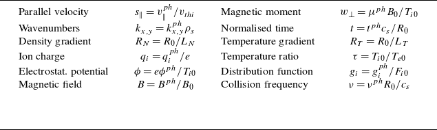


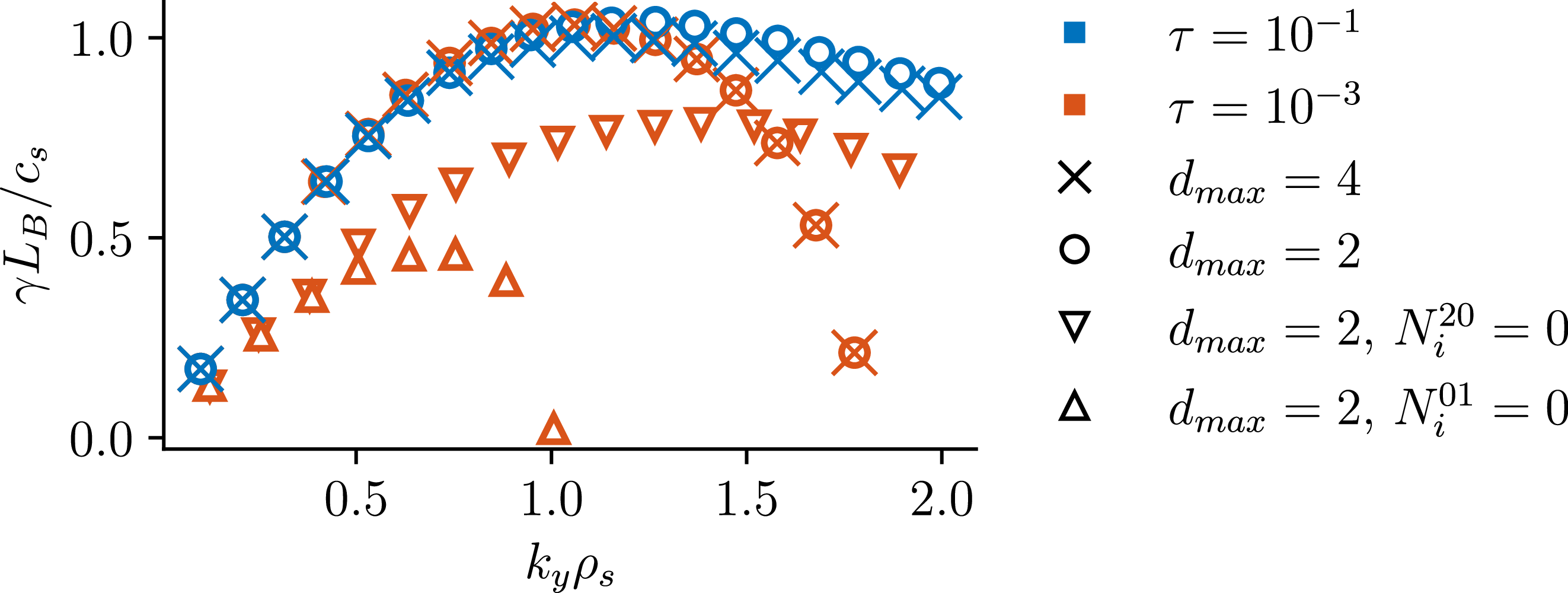


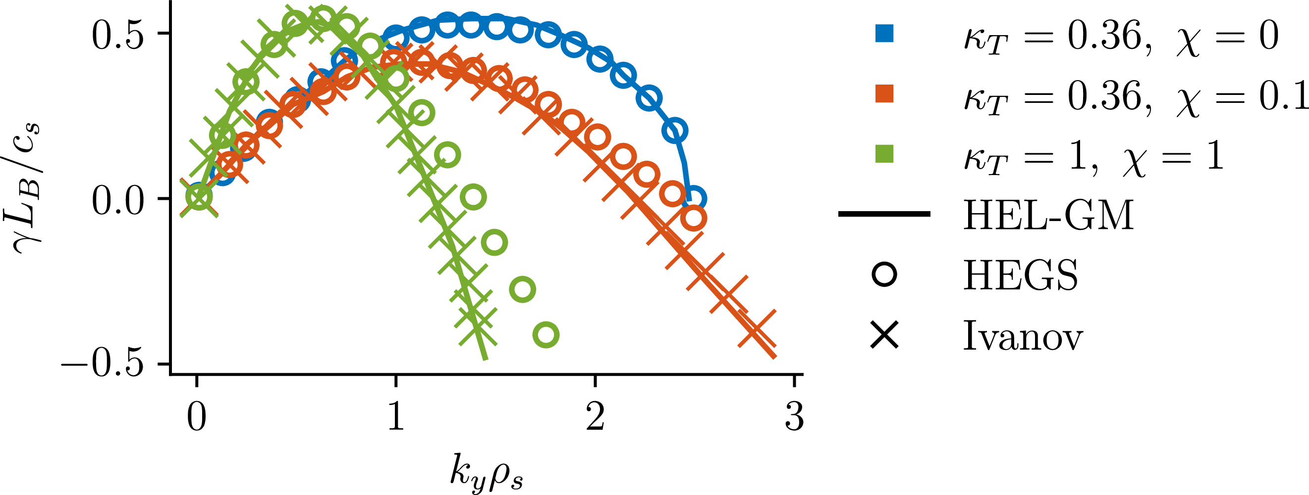


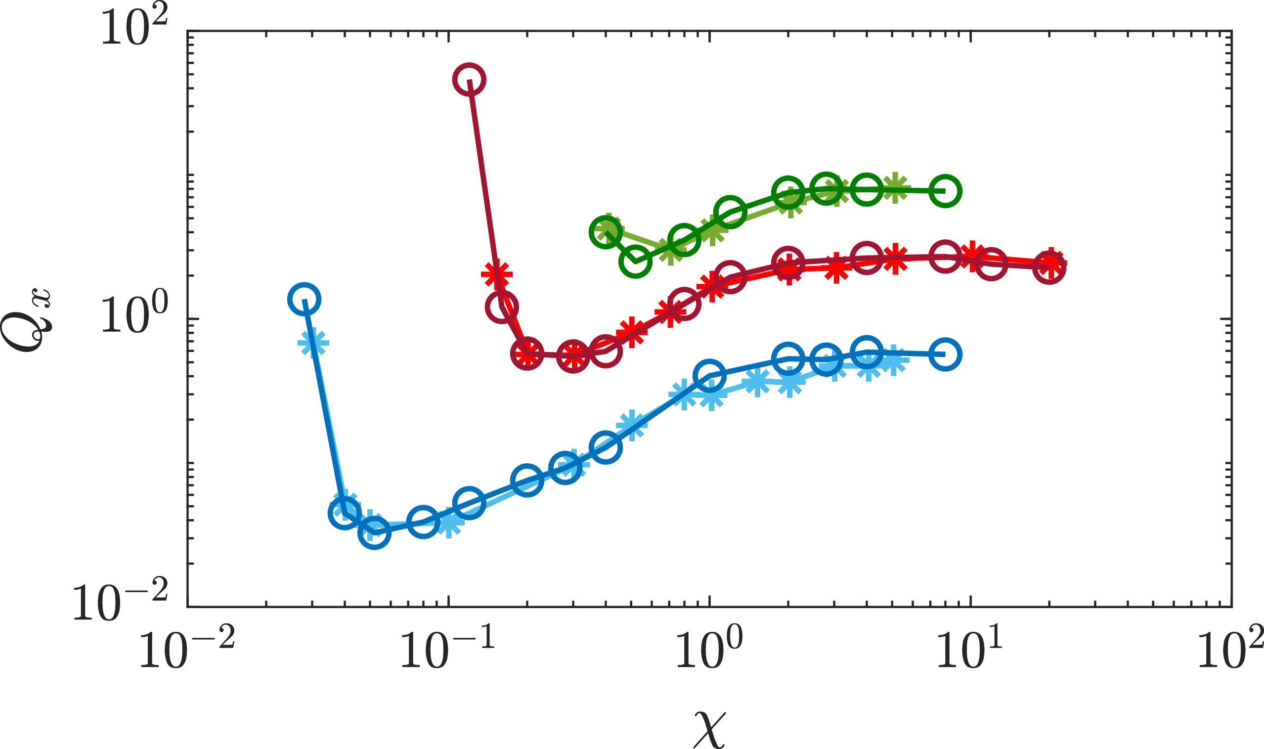


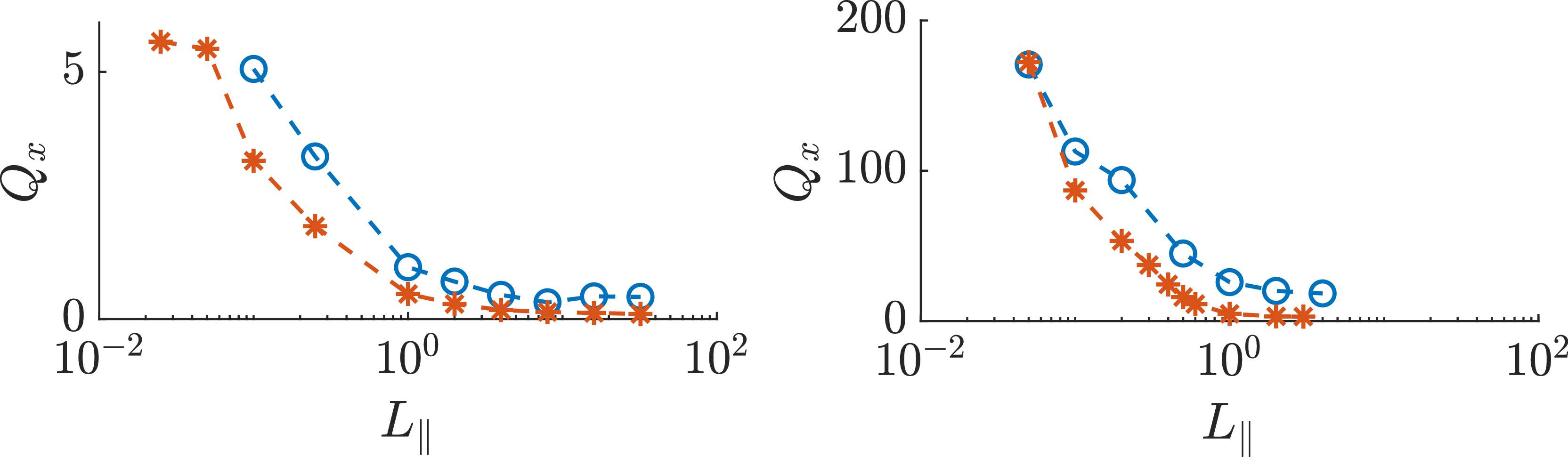


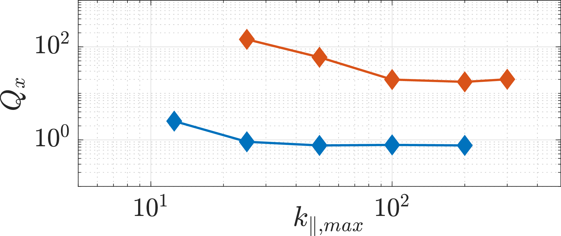


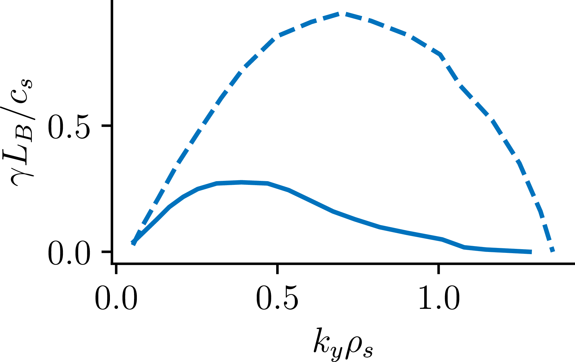

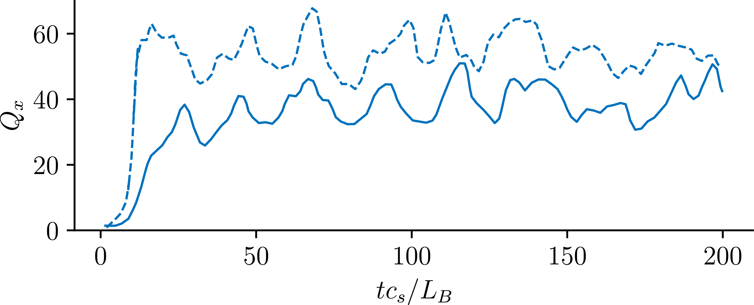
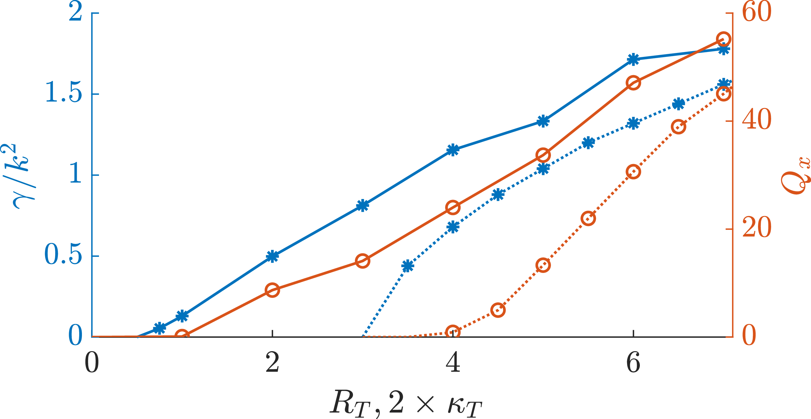

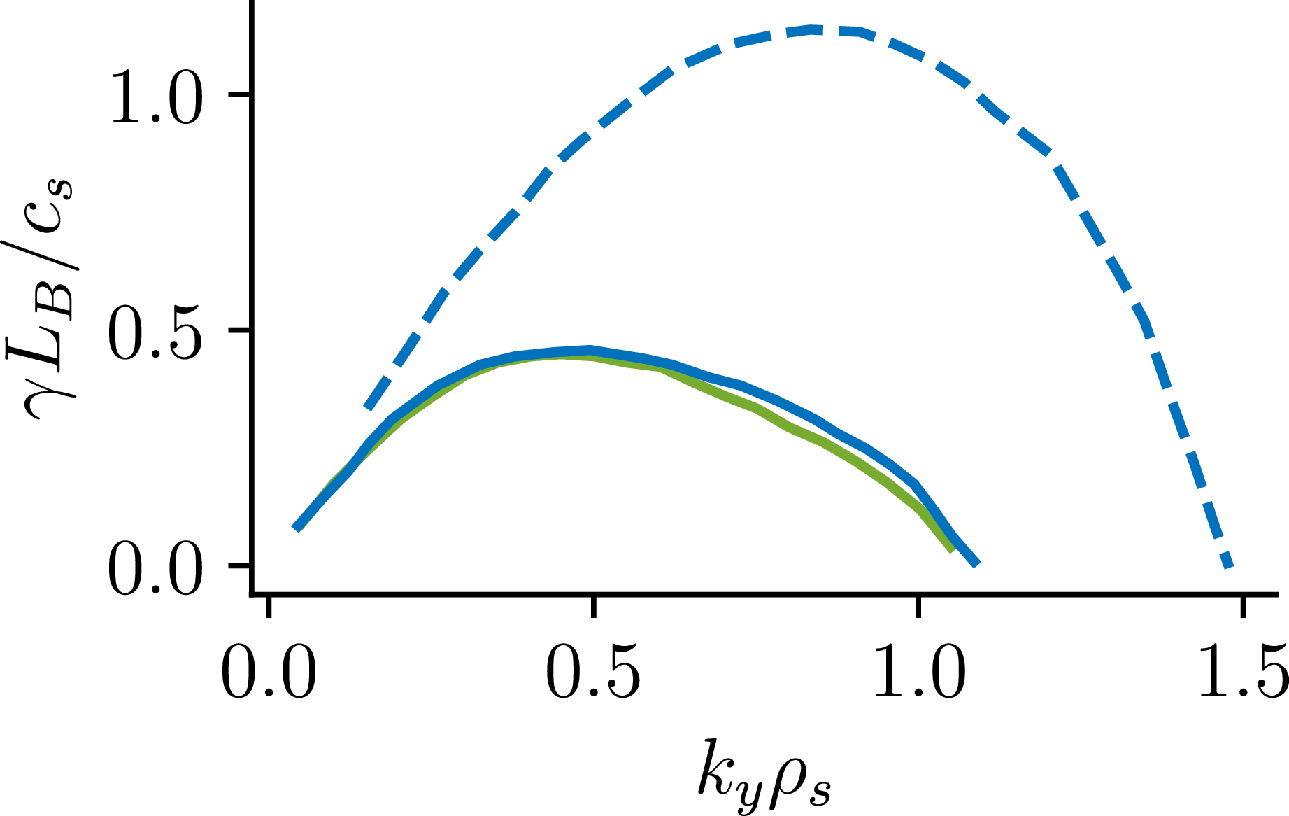


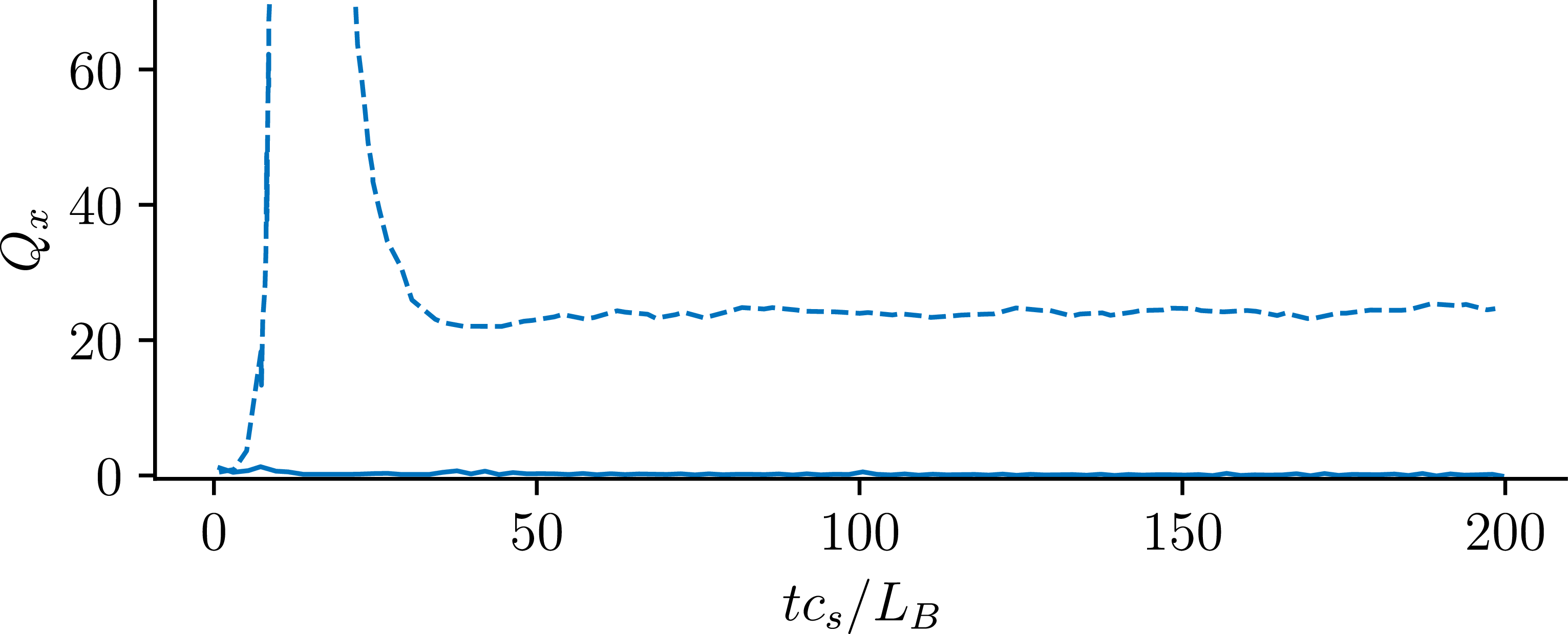

 Open access

