2.1. Experimental set-up

A schematic representation of the experimental apparatus is shown in figure 1. Figure 1(a) gives an overview of all the main components, including the measurement set-up (discussed later, in § 2.2), while figure 1(b) focuses on the near-field flow region of the mixing layer, i.e. immediately after the nozzle exit section, which is located at $x=0$. A water stream flows along the streamwise direction ($x$) below a parallel faster air stream, the two fluids being separated initially by a stainless steel splitter plate with thickness $e=2$ mm (figure 1b). The shapes of the water and air channels are the same. The walls are made from Plexiglas, with cross-sectional area (in the $yz$ plane) initially $100\,\text {mm}\times 100\,\text {mm}$ (where $y$ and $z$ are the normal-to-flow and spanwise coordinates, respectively). Then a two-dimensional converging nozzle reduces the channel height from 100 mm to $H_g = H_l = 20$ mm at $x=0$ (see table 1), where the flows issue into a test section. Three-dimensional effects due to the lateral confinement of the test section walls on the liquid jet are negligible in the near-field region of the flow, where the two-dimensional PIV measurements are realized.

Figure 1.

(a) Overall schematic representation and (b) two-dimensional sketch close to the nozzle exit section of the experimental set-up. In (b), the PIV measurement region of interest is highlighted in green.

Table 1.

Relevant geometrical quantities of the experimental set-up (see also figure 1b).

An overflow tank (figure 1a) positioned 1.5 m above the splitter plate drives the liquid flow by gravity, and is filled up continuously by a pump (T.I.P. TVX 12 000 Dompelpomp), thus realizing a closed-loop circuit for the water stream. At the end of the test section, the liquid flow spills out into a water collector. The flow rate, which is kept constant during each experiment, is regulated by means of a valve located upstream of the water channel entry; different values measured by a LVB-25-A vortex flowmeter are obtained, corresponding to liquid inlet velocities in the range $U_l \in [0.10,0.30]$ m s$^{-1}$. For each liquid flow rate value, the height of the water stream at the splitter plate edge (i.e. at $x=0$) is kept constant (equal to $H_l$) by adjusting the height of a gate placed at the end of the test section ($x=500$ mm), before the liquid is dispensed into a collector. In this way, air ingestion into the water channel at the splitter plate edge is avoided for all the testing conditions.

The air stream is generated by a blowing machine (Rück Ventilatoren RS315LEC) allowing us to obtain injection velocities in the range $U_g \in [2,15]$ m s$^{-1}$, as measured by a Pitot tube located at the gas nozzle exit section midpoint (i.e. at $x=0$, $y = 10$ mm), and cross-checked by static pressure probes positioned at the inlet ($x=-250$ mm) and outlet ($x=0$) sections of the convergent nozzle. Flow conditioners are used in both the liquid and gas channels to damp velocity fluctuations; two aluminum honeycombs (aluNID from Alucoat) with 50 mm long hexagonal cells are employed in the liquid phase, while a combination of the same honeycomb and mesh screens is used in the air channel.

Particular care is taken in designing the flow conditioners for the gas phase to control its turbulence intensity level, which has been shown to affect the mixing layer development in both experimental (Matas et al. Reference Matas, Marty, Dem and Cartellier2015) and numerical (Jiang & Ling Reference Jiang and Ling2020,  Reference Jiang and Ling2021) studies, and that depends strongly on screen geometrical properties and relative streamwise spacing in a multiple screens configuration (see, for example, the works by Mehta & Bradshaw Reference Mehta and Bradshaw1979; Marshall Reference Marshall1985; Groth & Johansson Reference Groth and Johansson1988). Following Groth & Johansson (Reference Groth and Johansson1988), we chose a combination of metal meshes (figure 1b), with mesh size decreasing progressively from $1$ mm (coarse screen) to $0.5$ mm (fine), and constant relative spacing $d=20$ mm, while a distance $D_g = 50$ mm was selected between the honeycomb and the first (i.e. located more upstream) coarse screen (see table 1). This configuration gives a turbulence intensity level below 1 % for all the testing conditions, as reported in figure 2(a). The turbulence intensity is quantified in terms of root mean square (rms) of the gas velocity fluctuation $u^\prime (t)= u(t) - \bar {u}$, where $u(t)$ is the streamwise velocity component measured (in absence of liquid stream) by a hot wire located at the gas nozzle exit section midpoint, and $\bar {u}$ its time-averaged value. Note that the values of the gas turbulence intensity reported here are close to the lowest value ($u^\prime _{rms}/\bar {u} = 0.8\,\%$) found by Matas et al. (Reference Matas, Marty, Dem and Cartellier2015) in their experimental analysis of the gas turbulence effect on the dynamics of an air–water mixing layer. Moreover, Matas et al. (Reference Matas, Marty, Dem and Cartellier2015) found that the peak frequency of the air–water interface oscillations was influenced by the gas turbulence only for values $u^\prime _{rms}/\bar {u} > 3.5\,\%$. Therefore, we can assert that results reported in the present work are not influenced by the turbulence intensity level of the gaseous phase.

Figure 2.

(a) Air flow turbulence intensity level $u^\prime _{rms}/\bar {u}$, and (b) inlet gas vorticity thickness $\delta _g$, varying with gas Reynolds number $Re_{H_g}$. Comparisons with past works are also reported in (b). (c) An overview of the testing conditions in terms of dynamic pressure ratio $M$ values as a function of the gas velocity $U_g$ at different liquid velocities $U_l$.

Reynolds number values reported in figure 2(a) correspond to $U_g = 2, 5, 7, 10, 12,$ $15$ m s$^{-1}$, the Reynolds number here being defined as $Re_{H_g} = \rho _g U_g H_g / \mu _g$, where $\rho _g$ and $\mu _g$ are respectively the gas density and dynamic viscosity. The inlet gas vorticity thickness $\delta _g$, which is defined as $\delta _g = {\rm \Delta} \bar {u}/({\rm d} \bar {u}/{{\rm d}y})|_{max}$ (${\rm \Delta} \bar {u} = \bar {u}(y=H_g/2)-\bar {u}(y=e/2)$) and is known to play a crucial role in the mixing layer instability selection mechanisms (Matas et al. Reference Matas, Marty and Cartellier2011; Fuster et al. Reference Fuster, Matas, Marty, Popinet, Hoepffner, Cartellier and Zaleski2013), has also been measured by positioning the hot wire at a downstream distance $x=e/2$. The obtained values are reported in figure 2(b) as a function of $Re_{H_g}$, revealing a good agreement with the scaling law $\delta _g / H_g = 5.2/ \sqrt {Re_{H_g}}$ proposed by Fuster et al. (Reference Fuster, Matas, Marty, Popinet, Hoepffner, Cartellier and Zaleski2013). An overview of the testing conditions considered in this work is summarized in figure 2(c), where liquid and gas injection velocities are reported together with the corresponding dynamic pressure ratio $M = \rho _g U^2_g/(\rho _l U^2_l)$ values.

2.2. Measurement technique

The single-laser single-camera measurement system designed to achieve the TR-PIV characterization of the flow simultaneously in the two phases is shown schematically in figure 1(a). As discussed in the Introduction, performing this type of measurement is challenging, and other strategies such as combining PIV with laser-induced fluorescence (Buckley & Veron Reference Buckley and Veron2017) or employing multi-camera multi-laser configurations (Kosiwczuk et al. Reference Kosiwczuk, Cessou, Trinitè and Lecordier2005; Ayati et al. Reference Ayati, Kolaas, Jensen and Johnson2014) have been explored to date. The major issues are related to the laser light reflection and refraction across the interface, and to the high velocity difference between the two phases (about two orders of magnitude).

In the present work, to enlighten simultaneously air and water flows overcoming light reflections at the interface, a Continuum Mesa PIV 532-120M laser operated at 2 kHz double pulse rate (pulse energy 18 mJ) is used to generate a light beam, which is then separated into two beams by a prism. The first beam goes through a combination of two spherical and one cylindrical lenses and a mirror, thus becoming a thin sheet enlightening the liquid phase. The second beam is rotated horizontally by a mirror, and is transformed into an analogous sheet for the air flow by the same combination of lenses and mirror. A high-speed (2 kHz repetition rate in double exposure mode) camera (Photron, Fastcam SA-1, $1024\times 1024$ pixels), whose axis is orthogonal to the laser sheets plane, and a programmable timing unit (LaVision, HSC, not shown in figure 1), complete the measurement set-up. Atomized droplets (mean diameter $1\,\mathrm {\mu } \text {m}$) are seeded in the air channel by a fog generator (SAFEX, Fog 2010+) using a working fluid of water–glycol mixture, while a $20\,\mathrm {\mu }\text {m}$ polyamide Vestosint powder is used to seed the liquid phase.

A field of view $[-18,108] \times [-21,21]\,\text {mm}^2$ (shown qualitatively in green in figure 1b) is imaged by mounting a 105 mm objective (Nikon, Micro-Nikkor) on the high-speed camera, thus giving a two-dimensional region of interest within the $xy$ plane positioned midway from the channel side walls. By adjusting the camera focus, particle images approximately 2–3 px in diameter are obtained in both liquid and gas phases, as shown in the raw image reported in figure 3(a). An algorithm written in MATLAB is used to pre-process the raw images (figure 3b) and separate air and water phases (figures 3c,d), which are then post-processed separately through LaVision DaVis 10. An iterative multi-grid cross-correlation scheme with window deformation (Scarano & Riethmuller Reference Scarano and Riethmuller2000) is used to compute velocity fields, and results are post-processed with the universal outlier detection algorithm (Westerweel & Scarano Reference Westerweel and Scarano2005). The time delay between two successive frames in air is adjusted from ${\rm \Delta} t_g=200\,\mathrm {\mu }$s to ${\rm \Delta} t_g=70\,\mathrm {\mu }$s for $U_g \in [2, 15]$ m s$^{-1}$, while values ranging from ${\rm \Delta} t_l=10.5$ ms to ${\rm \Delta} t_l=1.2$ ms are employed for cross-correlation in water ($U_l \in [0.10, 0.30]$ m s$^{-1}$), to guarantee a peak particle displacement of approximately 10 pixels in both phases. For each pair of $U_g$ and $U_l$ values, the time delay ${\rm \Delta} t_l$ for cross-correlation in water is adjusted simply by skipping the number of frames necessary to achieve the same peak particle displacement as in air, i.e. $U_l\, {\rm \Delta} t_l = U_g\,{\rm \Delta} t_g$. In the final pass of the cross-correlation operation, the interrogation window size and the overlapping ratio are $16\,{\rm px} \times 16\,{\rm px}$ and 50 %, respectively, leading to spatial resolution 1 mm per vector. Mean quantities are estimated based on $N_t=8000$ realizations, with average measurement uncertainty on the streamwise and normal-to-flow velocity components respectively in the ranges $[0.62, 9.43]$ % and $[0.71, 6.28]$ % of the injection velocities (increasing value moving towards walls).

Figure 3.

Single-laser single-camera PIV measurement workflow: (a) acquired raw image, (b) pre-processing, and (c,d) phase separations.

The PIV measurements allow us to complement the air stream characterization in terms of inflow conditions as shown in figure 4. In particular, the mean streamwise velocity component profile $\bar {u}$ is shown at three different streamwise stations upstream of the injection section: $x/H_g = -1$ (figure 4a), $x/H_g = -0.5$ (figure 4b) and $x/H_g = -0.1$ (figure 4c). Note that the normal-to-flow coordinate $y$ has been shifted by $e/2$ ($y^\star = y -e/2$), such that $\bar {u} = 0$ at $y^\star = 0$, and $\bar {U}_g$ denotes the mean velocity at each station. Three velocity profiles are reported in each panel, corresponding to $Re_{H_g} = 6.7\times 10^{3}$ (black curves), $9.6\times 10^{3}$ (red curves) and $16.2\times 10^{3}$ (blue curves), and the numerical solution of the fully developed turbulent channel flow obtained by Kim et al. (Reference Kim, Moin and Moser1987) at Reynolds number 13 750 is also reported for comparison (green curve). The velocity profile tends to the fully developed turbulent channel flow solution as $Re_g$ increases, thus highlighting a transition towards turbulent inflow conditions. This occurrence seems to be confirmed by the trend of the turbulence intensity reported in figure 2(a), showing an initially increasing behaviour followed by a plateau. Of course, each velocity profile is not symmetric with respect to the $y$ direction, due to the intrinsic shape of the exit nozzle, limited by the flat splitter plate and the converging lateral wall (where the boundary layer is thinner).

Figure 4.

Velocity profile in air at different streamwise stations upstream of the injection section by varying the Reynolds number: $Re_{H_g} = 6.7\times 10^{3}$ (black curves), $Re_{H_g}=9.6\times 10^{3}$ (red curves), $Re_{H_g} = 16.2\times 10^{3}$ (blue curves). The numerical solution of the fully developed turbulent channel flow obtained by Kim, Moin & Moser (Reference Kim, Moin and Moser1987) at Reynolds number 13 750 is also reported for comparison (green curve).

3.1. The REF case

The time-averaged velocity magnitude $\bar {V}$ contour is shown in figure 5(a) together with the velocity vectors distribution, and a zoom around the splitter plate immediately downstream of the nozzle exit section is provided in figure 5(b). For all cases discussed within this work, the mean quantities $\bar {u}$ and $\bar {v}$ are computed over a total of 8000 temporal realizations of the flow.

Figure 5.

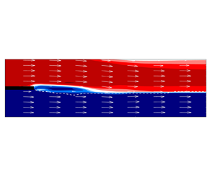
(a) Time-averaged velocity magnitude $\bar {V}/U_g$ contour, with (b) zoom next to the nozzle exit section. The splitter plate is highlighted in black, the time-averaged interface location is represented as a white dashed line, and velocity vectors are also reported. REF case of table 3.

Note that in figure 5, the velocity magnitude has been scaled with respect to $U_g$, the spatial coordinates have been made dimensionless by means of the splitter plate thickness, i.e. $\tilde {x} = x/e$ and $\tilde {y} = y/e$, and the time-averaged interface location has been represented as a white dashed line. Moreover, here as elsewhere, velocity vectors in the liquid phase have been magnified by a factor of ${O}(10^2)$.

After issuing from the injection section ($\tilde {x}=0$), the air and water flows meet downstream of the splitter plate. By moving along the streamwise direction, two distinct regions can be detected: a wake ($0<\tilde {x}<\tilde {x}_w$) and a pure mixing layer ($\tilde {x} > \tilde {x}_w$) region, with $\tilde {x}_w = x_w/e = 17.5$. The wake region length $\tilde {x}_w$ has been calculated as the last streamwise station (starting from $\tilde {x}=0$) where $\bar {u}(\tilde {y}) < 0$ (i.e. $\bar {u} > 0$ for $\tilde {x} > \tilde {x}_w$). The spatial development of the mixing layer is more clearly quantified in figure 6, which reports $\bar {u}(\tilde {y})$ profiles at different streamwise stations spanning both air and water streams, together with the corresponding average measurement uncertainty. The reverse flow component within the wake region is highlighted by the negative values of $\bar {u}$ for $\tilde {y}$ around zero. Far from $\tilde {y}=0$, the velocity profile is characterized by an almost uniform distribution in both air ($\tilde {y} > 2$) and water ($\tilde {y} < -1.1$) streams, while it undergoes strong spatial variations within the region $-1.1<\tilde {y} < 2$. Downstream of the wake region, the velocity profile is influenced by the air–air mixing layer forming between the injected gas stream and the external still ambient, with consequent reduction of the local $\bar {u}$ value by increasing $\tilde {y}$ (phenomenon of jet expansion; see Descamps et al. Reference Descamps, Matas and Cartellier2008).

Figure 6.

Time-averaged streamwise $\bar {u}(\tilde {y})/U_g$ velocity component profiles at different $\tilde {x}$ stations: $0.55$ (black circles), $10.88$ (red diamonds), $21.76$ (blue squares), $32.10$ (black stars), $42.98$ (red triangles), $53.31$ (blue circles). The dashed and dotted lines represent the values $\bar {u}/U_g = 0$ and $1$, respectively, and error bars denote the average measurement uncertainty, while green circles highlight the interface location. REF case of table 3.

By moving along $\tilde {x}$, the momentum exchange between the faster gas and the slower water stream leads to the progressive reduction of the velocity deficit, which is the difference between the minimum and the free-stream local liquid velocities ($\bar {u}_{min} - U_l$). This aspect is clarified in figure 7, which shows the velocity profile at three selected downstream stations, respectively inside ($\tilde {x} = 0.55$, black curve), just outside ($\tilde {x} = 20.13$, red curve) and far from ($\tilde {x} = 53.31$, blue curve) the wake region (figures 7a,b), and the velocity deficit streamwise distribution (figure 7c), together with the corresponding average measurement uncertainty.

Figure 7.

(a) Time-averaged streamwise $\bar {u}(\tilde {y})/U_g$ velocity component profiles at different $\tilde {x}$ stations, with (b) zoom near the liquid phase, and (c) velocity deficit $(\bar {u}_{min} - U_l)/U_g$ streamwise distribution. In (c), the vertical red line denotes the wake region length $\tilde {x}_w$, the horizontal blue dashed line denotes the zero, and error bars represent the average measurement uncertainty. REF case of table 3.

The different regions characterizing the flow topology are further highlighted by $\bar {u}(\tilde {x})$ and $\bar {v}(\tilde {x})$ velocity profiles, shown respectively in figures 8(a,b), for normal-to-flow stations spanning both air and water streams. The distribution $\bar {u}(\tilde {x},\tilde {y}=0)$ highlights the strong spatial variation characterizing the flow field in the wake region (blue curve in figure 8a), while $\bar {v}(\tilde {x})$ profiles reveal the downward deviation of the gas stream (i.e. negative values of $\bar {v}(\tilde {x})$) in the near-field region, as a result of the combination of water jet contraction (Agbaglah et al. Reference Agbaglah, Chiodi and Desjardins2017) and air recirculation within the wake.

Figure 8.

(a) Time-averaged streamwise $\bar {u}(\tilde {x})/U_g$ and (b) normal-to-flow $\bar {v}(\tilde {x})/U_g$ velocity component profiles at different $\tilde {y}$ stations. REF case of table 3.

Figures 9 and 10 show the Reynolds stress tensor components $\overline {u^\prime u^\prime }$, $\overline {v^\prime v^\prime }$ and $\overline {u^\prime v^\prime }$ in terms of contour representations and $\tilde {y}$ profiles, respectively. The $\tilde {x}$ velocity component fluctuation is evaluated as $u^\prime = u - \bar {u}$, and the same applies for $v^\prime$. The $\overline {u^\prime u^\prime }(\tilde {y})$ distribution (figures 9a and 10a) is characterized by larger peaks than the others (figures 9b,c and 10b,c), as also found by Ling et al. (Reference Ling, Fuster, Tryggvason and Zaleski2019) by means of three-dimensional direct numerical simulations. Moreover, all the distributions are peaked in correspondence with the maximum momentum exchange locations, namely at the air–water and air–air mixing layers (the latter on the image top), as already evidenced in discussing figure 6 (see also Jiang & Ling Reference Jiang and Ling2021). Similarly, the streamwise $\overline {u^\prime u^\prime }(\tilde {x})$ distribution reported in figure 10(d) reveals two peaks, the first immediately downstream of the splitter plate, and the second at $\tilde {x}_w = 17.5$, namely at the end of the recirculation region. It is also possible to appreciate that for each $\tilde {y}$ location, a constant value is approached asymptotically as $\tilde {x}$ increases, revealing that the mixing layer progressively achieves a self-similar state moving far from the wake region (Mehta Reference Mehta1991).

Figure 9.

Contours of (a) $\overline {u^\prime u^\prime }/U^2_g$, (b) $\overline {v^\prime v^\prime }/U^2_g$ and (c) $\overline {u^\prime v^\prime }/U^2_g$. The splitter plate is highlighted in black, while the white dashed line denotes the time-averaged interface location. REF case of table 3.

Figure 10.

Profiles of (a) $\overline {u^\prime u^\prime }/U^2_g$, (b) $\overline {v^\prime v^\prime }/U^2_g$ and (c) $\overline {u^\prime v^\prime }/U^2_g$ at different streamwise stations $\tilde {x}$: $0.55$ (black circles), $21.76$ (red diamonds), $53.31$ (blue triangles). (d) Profiles of $\overline {u^\prime u^\prime }/U^2_g$ at different $\tilde {y}$ stations. REF case of table 3.

The analysis of the REF case is concluded by reporting a comparison between the measured velocity profiles and the theoretical base flows proposed by Otto et al. (Reference Otto, Rossi and Boeck2013) and Fuster et al. (Reference Fuster, Matas, Marty, Popinet, Hoepffner, Cartellier and Zaleski2013) in the context of the local stability analysis. The comparison is performed at two distinct streamwise stations: the first inside the wake region ($\tilde {x} < \widetilde {x_w}$, figures 11a,b), and the second just outside it ($\tilde {x} > \widetilde {x_w}$, figures 11c,d). Note that the measured profiles (black curves) have been represented by employing the shifted coordinate $y^\star$, defined previously in § 2.2, to facilitate the comparisons with theoretical formulae (red curves) provided hereafter.

Figure 11.

Theoretical–experimental comparison of velocity profiles (a,b) inside ($\tilde {x}=0.55$) and (c,d) outside ($\tilde {x}=20.13$) the wake region of length $\tilde {x}_w=17.5$. REF case of table 3.

The analytical velocity profile used in figures 11(c,d) reads as

(3.2) \begin{equation} \frac{u^+}{U_m} = \begin{cases} -\dfrac{U_l}{U_m}\,\text{erf} \left(\dfrac{y^\star}{\delta_l}\right) + \dfrac{\bar{u}_0}{U_m} \left[1 + \text{erf} \left(\dfrac{y^\star}{\delta_d}\right)\right], & y^\star{\leq} 0,\\ \dfrac{U_g}{U_m}\,\text{erf} \left(\dfrac{y^\star}{\delta_g}\right) + \dfrac{\bar{u}_0}{U_m} \left[1 - \text{erf} \left(\dfrac{y^\star}{\delta_d}\right)\right], & y^\star{\geq} 0, \end{cases} \end{equation}

which is the same as that reported by Fuster et al. (Reference Fuster, Matas, Marty, Popinet, Hoepffner, Cartellier and Zaleski2013) once small notational differences are rectified, while a modified version (discontinuous at $y^\star =0$) is adopted for comparisons in the wake region (figures 11a,b),

(3.3) \begin{equation} \frac{u^-}{U_m} = \begin{cases} -\dfrac{U_l}{U_m}\,\text{erf} \left(\dfrac{y^\star}{\delta_l}\right) + \dfrac{\bar{u}_0}{U_m} \left[1 + \text{erf} \left(\dfrac{y^\star}{\delta_d}\right)\right], & y^\star{\leq} 0,\\ \dfrac{U_g}{U_m}\,\text{erf} \left(\dfrac{y^\star{-}y^\star_{min}}{\delta_g}\right) + \dfrac{\bar{u}_{min}}{U_m} \left[1 - \text{erf} \left(\dfrac{y^\star{-}y^\star_{min}}{\delta_d}\right)\right], & y^\star{>} 0. \end{cases}\end{equation}

In (3.2)–(3.3), the error function $\text {erf}(y^\star )$ is employed, $U_m = (U_g + U_l)/2$, $\bar {u}_0$ is the measured velocity at the air–water interface (an analytical estimation based on continuity of shear stresses across the interface was used by Fuster et al. Reference Fuster, Matas, Marty, Popinet, Hoepffner, Cartellier and Zaleski2013), $\bar {u}_{min}$ is the minimum (negative) measured value within the wake region (at the location $y^\star = y^\star _{min}$), and $\delta _d$ is an adjustable parameter introduced by Otto et al. (Reference Otto, Rossi and Boeck2013) to mimic experimental velocity profiles in the near-field region of the mixing layer.

Results of the comparison reveal a strict agreement between the measured and theoretical velocity profiles, both inside (i.e. negative value of velocity deficit) and outside the wake region. Values of the ratio $\delta _d/\delta _g$ giving the best match with experimental data are respectively $0.75$ (for $\tilde {x} < \tilde {x}_w$) and $0.78$ ($\tilde {x} > \tilde {x}_w$). In agreement with Otto et al. (Reference Otto, Rossi and Boeck2013), we have $\delta _d/\delta _g < 1$ in both cases, due to the presence of a velocity deficit in the mean flow profile.

3.2. Effect of liquid Reynolds number

The effect of the liquid Reynolds number $Re_l$ variation on the two-phase flow topology at fixed $Re_g$ is investigated by modifying the injection velocity $U_l$. Results are shown in figure 12, where $\bar {u}(\tilde {y})$ distributions at different streamwise stations are reported for the REF and L3 cases, and in figure 13 in terms of time-averaged velocity magnitude contours and vectors distribution. The liquid Reynolds number varies between $Re_l=302$ (L1 case) and $Re_l = 807$ (L3 case), while the gas Reynolds number is $Re_g = 493$, as in the REF case discussed previously.

Figure 12.

Liquid Reynolds number $Re_l$ effect on the time-averaged streamwise $\bar {u}(\tilde {y})/U_g$ velocity component at different $\tilde {x}$ stations: $0.55$ (black circles), $21.76$ (red diamonds), $53.31$ (blue triangles). Cases (a) REF and (b) L3 of table 3.

Figure 13.

Liquid Reynolds number $Re_l$ effect on the time-averaged velocity magnitude $\bar {V}/U_g$. The mean interface location is represented as a white dashed line, and velocity vectors are also reported. Cases (a) L1, (b) REF, (c) L2 and (d) L3 of table 3.

The velocity maps reported in figure 13 show that the recirculation region characterizing the flow immediately downstream of the injection section progressively reduces as $Re_l$ increases, until it vanishes in the last (L3) case. The increase in inlet velocity of the liquid phase produces a shear effect at the interface, which accelerates locally the (transitional) gas flow and determines the progressive absorption of the wake. For the L3 case, the absence of the wake flow component determines an almost unperturbed air–water interface at the splitter plate edge. As a consequence, the two-phase mixing layer flow becomes spatially invariant along the streamwise direction up to $\tilde {y}=5$ (see figure 12b), where differences among the streamwise-spaced velocity profiles are due to the presence of the air–air mixing layer, as observed previously in § 3.1.

It is important to note that when no wake is present due to a high $Re_l$ value, the liquid velocity field is basically not influenced by the co-flowing gaseous phase, developing parallel to the streamwise direction and to the injected air stream (figure 13d). This aspect will be highlighted further in § 3.3, where the effect of the gas Reynolds number on the variation of the flow topology will be presented and compared with the present discussion. A complete parametric trend of the wake length as a function of $Re_l$ for various $Re_g$ values will also be shown in § 3.3.

3.3. Effect of gas Reynolds number

Results of the investigation performed by varying the gas Reynolds number are first shown in figures 14 and 15, respectively in terms of velocity magnitude contours with superposed vectors distributions, and $\bar {u}(\tilde {y})$ profiles at different streamwise locations; the liquid velocity is kept constant and equal to that of the REF case, so that $Re_l = 454$.

Figure 14.

Gas Reynolds number $Re_g$ effect on the time-averaged velocity magnitude $\bar {V}/U_g$. The mean interface location is represented as a white dashed line, and velocity vectors are also reported. Cases (a) G1, (b) REF, (c) G3 and (d) G4 of table 3.

Figure 15.

Gas Reynolds number $Re_g$ effect on the time-averaged streamwise $\bar {u}(\tilde {y})/U_g$ velocity component at different $\tilde {x}$ stations: (a) $0.55$, (b) $21.76$, (c) $53.31$. Cases G1 (black circles), REF (red diamonds), G3 (blue triangles) and G4 (green squares) of table 3.

By looking at the two-dimensional flow fields in figures 14(a–c) and the velocity profiles in figure 15(a), it can be seen that the wake region shortens progressively by increasing $Re_g$ from the G1 to the G3 case, with $\tilde {x}_w$ decreasing from $21.2$ to $9.8$. Accordingly, the peak of the Reynolds stress component $\overline {u^\prime u^\prime }$ is shifted towards lower $\tilde {x}$ values, and it achieves its maximum at $Re_g=704$ (G2 case of table 3), as reported in figure 16. Due to the sudden change of the shear boundary condition downstream of the plate, the liquid velocity relaxes, and the water jet accelerates progressively and contracts along the streamwise direction $x$ (Tillett Reference Tillett1968), as can be appreciated by looking at figures 14(a,b,c) in turn. Moreover, outside the wake region, the gas jet goes down progressively as $Re_g$ increases (see also Agbaglah et al. Reference Agbaglah, Chiodi and Desjardins2017). The momentum flux difference in the air–air mixing layer also increases by increasing $Re_g$, leading to a reduction in $\bar {u}(\tilde {y})$ moving towards the top of the domain, as shown by the evolution of velocity profiles in figures 15(b,c).

Figure 16.

Profiles of $\overline {u^\prime u^\prime }/U^2_g$ at $\tilde {y} = 0$ for different values of the gas Reynolds number, for cases REF (black curve), G2 (red curve) and G4 (blue curve) of table 3.

For the highest value of gas Reynolds number considered (G4 case, see figure 14(d) and green curves in figure 15), the wake region vanishes, i.e. $\tilde {x}_w = 0$. As a consequence, no peak in the Reynolds stress component $\overline {u^\prime u^\prime }$ distribution is detected (blue curve in figure 16). It is important to note that when $\tilde {x}_w = 0$ due to a high $Re_g$ value, the flow topology is significantly different from the case $\tilde {x}_w = 0$ at high $Re_l$ discussed previously in § 3.2, as can be appreciated by comparing figures 14(d) and 13(d). As a matter of fact, the momentum exchanged by shear at the interface between the gas and liquid jets as $Re_g$ increases accelerates the liquid, which then has to contract to conserve the mass flow rate (figure 14d). As a consequence, the flow is no longer spatially invariant along the streamwise direction, as instead it has been observed at high $Re_l$ value (figure 13d).

An overall picture of the wake extension variation with $Re_l$ and $Re_g$ parameters is given in figure 17, where the trend $\tilde {x}_w(Re_l)$ is reported for different values of the gas Reynolds number $Re_g$, corresponding to the flow fields shown in figures 13 and 14. Note that additional cases characterized by a lower gas Reynolds number ($Re_g=256$) have also been reported (black curve in figure 17). It can be seen that the progressive decreasing of the recirculation region with $Re_l$ is enhanced by increasing the gas Reynolds number. At $Re_g = 768$, no wake is detected for any value greater than $Re_l=302$ (orange curve in figure 17). The trend $\tilde {x}_w(Re_l)$ is qualitatively the same for all the other $Re_g$ values: it is approximately constant up to $Re_l = 454$, then it decreases, reaching zero value for $Re_l = 807$.

Figure 17.

Liquid Reynolds number $Re_l$ effect on the wake region length $\tilde {x}_w$ at different $Re_g$ values.

3.4. Effect of gas-to-liquid dynamic pressure ratio

Finally, the trend of the wake length as a function of the gas-to-liquid dynamic pressure ratio $M$ is summarized in figure 18, for different values of the gas Reynolds number. It can be seen that for a fixed $Re_g$, relatively low $M$ values (high liquid velocities) promote a reduction of the wake, which vanishes eventually. This is analogous to the $Re_l$ effect outlined in figure 17 and by the velocity contours reported in figure 13. Moreover, the $M$ value denoting the transition from a wake regime to a pure mixing layer regime increases with $Re_g$. Therefore, only at relatively high values of the gas Reynolds number does the flow behave as a pure mixing layer in a wide range of liquid injection velocities (i.e. wide range of $M$ values).

Figure 18.

Dynamic pressure ratio $M$ effect on the wake region length $\tilde {x}_w$ at different values of the gas Reynolds number $Re_g$.

As a first summary of the results concerning the mean (time-averaged) flow analysis, a comprehensive characterization of the flow fields in both the phases has been described, including velocity profiles in various streamwise stations, Reynolds stress tensor components, and wake size. The measured velocity profiles agree well with analytical formulae proposed in past works for locally parallel flows in spatio-temporal stability analysis. The transition from a mixed wake mixing layer to a pure mixing layer regime as a function of the governing parameters has been highlighted. In § 4, which reports the unsteady flow characteristics, the dominant flow oscillations will be interpreted in connection with the velocity profiles and the overall flow topology analysed here, giving insights into the global dynamics of the gas–liquid interface.

4.1. Proper orthogonal decomposition and interfacial dynamics

To elucidate in more depth the spatio-temporal flow topology in presence of synchronized velocity oscillations, the analysis of the G5 case is broadened by performing a modal decomposition analysis, namely the POD of momentum fluctuations $\rho v^\prime$:

(4.1)\begin{equation} \rho\,v^\prime(\tilde{x},\tilde{y},t)= \rho\,v(\tilde{x},\tilde{y},t)- \overline{\rho v}\,(\tilde{x},\tilde{y}) =\sum_{j=1}^{\infty}a_j(t)\,\varphi_j(\tilde{x},\tilde{y}), \end{equation}

where the density $\rho$ is equal to $\rho _l$ ($\rho _g$) in the liquid (gas) phase (see table 2 in § 3). The gappy POD iterative algorithm (Everson & Sirovich Reference Everson and Sirovich1995; Venturi & Karniadakis Reference Venturi and Karniadakis2004; Gunes, Sirisup & Karniadakis Reference Gunes, Sirisup and Karniadakis2006) is applied to de-noise the data and extract the leading modes, with a spatial weight matrix (defining the state vector norm) accounting for the different densities of gas and liquid phases. The POD analysis is carried out in the spatial region $x \in [-5,30] \times y \in [-10,5]$, i.e. around the gas–liquid interface.

Results are reported in figure 24 in terms of energy distribution (figure 24a) and the topology of the leading five modes (figures 24b–f), and in figure 25, which shows the PSD of the corresponding temporal coefficients $a_i$. The first mode has a 23 % energy content and represents a normal-to-flow flapping motion of the interface (figure 24b). The PSD of the associated temporal coefficient $a_1$ reveals a peak frequency $f \delta _g/U_g = 2.8 \times 10^{-4}$ (figure 25), which is the same value found in the local spectral analyses shown previously in figure 22. This finding reveals that the synchronized velocity oscillations measured within the gas and liquid phases are determined by a flapping mode of the gas–liquid interface, which therefore rules the whole flow field dynamics. The other leading modes are associated with different flow coherent structures. In particular, the pair of 2nd and 3rd modes (containing 8.5 % and 7.2 % energy, respectively) and 4th and 5th modes (containing 5.4 % and 4.0 % energy, respectively) represent interfacial travelling waves advected along the streamwise direction, each couple being characterized by the typical shift of modes along the $\tilde {x}$ axis (figure 24c–f).

Figure 24.

POD analysis of the G5 case of table 3. (a) POD modes energy distribution (%). (b–f) Leading modes (1st to 5th, respectively, each scaled with respect to its maximum). In each plot, the splitter plate is highlighted in grey, and the mean interface location is denoted by the white dashed line.

Figure 25.

The PSD of the temporal coefficients $a_i$ associated with the leading POD modes shown in figure 24. The vertical red dashed lines denote the peak frequency $f \delta _g/U_g=2.8 \times 10^{-4}$ and its first super-harmonic $f \delta _g/U_g = 5.6\times 10^{-4}$.

To obtain an estimate of the order of magnitude of the flapping mode frequency, literature data measured in analogous flow configurations of separated flows past a backward facing ramp (Chiatto, luca & Grasso Reference Chiatto, de Luca and Grasso2021), or more generally in the presence of a separation bubble (Kiya & Sasaki Reference Kiya and Sasaki1983), have been considered, although these data were taken for bubbles forming in single phase flows. Following Chiatto et al. (Reference Chiatto, de Luca and Grasso2021), who expressed the Strouhal number in terms of the flow reattachment length, in the present context it has been assumed that the length of the flapping interface coincides with practically the entire length of the test section, i.e. $\lambda =250e$. As a consequence, it has been found that $St = f \lambda /U_g = {O}(10^{-1})$, which agrees well with values reported in the studies cited above.

It is interesting to note that multiplying the second POD mode wavelength $\lambda = 25 e$ (figure 24c) by the secondary peak frequency of the PSD ($a_2$), $f \delta _g/U_g = 5.6 \times 10^{-4}$ (figure 25), one can infer the dimensional velocity of the travelling disturbance wave, i.e. ${U}= \lambda f = 0.55$ m s$^{-1}$. This value is in close agreement with the interfacial wave propagation speed given by Dimotakis (Reference Dimotakis1986), $U_D = 0.59$ m s$^{-1}$ (relative spread 6.78 % for $U_l = 0.1$ m s$^{-1}$ and $U_g = 15$ m s$^{-1}$, corresponding to the G5 case analysed here), which was obtained assuming the gas and liquid dynamic pressures to be in balance in a reference frame moving with the wave speed. Moreover, the mode wavelength is of the same order as the gas injector size, namely $\lambda /H_g = 2.5$.

The synchronized velocity oscillations associated with the flapping mode in the G5 case are retrieved also in the G4 case, whose time-averaged flow shows no wake (as shown previously in figure 14d). This can be appreciated by looking at figures 26(a,b), respectively showing the flapping modes of the G5 and G4 cases (the modes energy distributions of the two cases are reported in figure 27, red and blue curves, respectively). Observe also that for the G4 case, the interface flapping is not associated with the presence of any wake. In general, the flapping mode occurs only at high $Re_g$ and $M$ values; as a matter of fact, none of the cases analysed here below the threshold value $M \approx 3$ exhibits this mode. Figure 27 shows also that both cases G5 and G4 feature a low-order behaviour. In summary, at high $Re_g$ values, independently of the presence of the wake, the dominant global flow structure is represented by the flapping mode of the interface, with oscillations synchronized in all the stations.

Figure 26.

The first POD modes of the cases (a) G5, (b) G4 and (c) REF of table 3. (d) The second POD mode of the REF case. In each plot, the splitter plate is highlighted in grey, the mean interface location is denoted by the white dashed line, and each mode is scaled with respect to its maximum.

Figure 27.

The POD modes energy distribution of the G5 (red curve), G4 (blue curve) and REF (black curve) cases of table 3.

For lower values of $Re_g$, the dominant structures are represented by a sort of fingers shedding, oscillating at higher frequency. This is shown for the REF case in figures 26(c,d) (the corresponding modes energy distribution is reported in figure 27, black curve). The pair of 1st and 2nd modes of the REF case represents a shedding mode of the gas phase, which is characterized by a dimensionless frequency $f \delta _g / U_g = {O}(10^{-2})$, significantly higher than the flapping dynamics frequency $f \delta _g / U_g = 2.8 \times {O}(10^{-4})$ identified previously. As a more general result, the low $Re_g$ regimes feature the presence of the wake, and the shedding of finger structures represents the dominant modes oscillating at higher frequency. For the REF case reported here, figure 27 indicates that the low-order behaviour is no longer valid, the energy being distributed almost evenly among the modes.