2. Guiding-centre motion in the presence of an Alfvénic perturbation

The guiding-centre motion, $\boldsymbol {R}(t)$, is described by the Lagrangian (Littlejohn Reference Littlejohn1983)

(2.1)\begin{equation} L(\boldsymbol{R},\dot{\boldsymbol{R}},v_{\|}) = q\left(\boldsymbol{A} + \frac{M v_{\|}}{q B}\boldsymbol{B} \right) \boldsymbol{\cdot} \dot{\boldsymbol{R}} - \frac{M v_{\|}^2}{2} - \mu B - q\varPhi, \end{equation}

where $q$ is the charge, $M$ is the mass, $v_{\|}$ is the velocity in the direction of the magnetic field, $\mu$ is the magnetic moment, $\varPhi$ is the electrostatic potential, and $\boldsymbol{A}$ is the vector potential. We assume the magnetic field is comprised of an equilibrium field, $\boldsymbol {B}_0$, and a shear Alfvénic perturbation (White et al. Reference White, Goldston, McGuire, Boozer, Monticello and Park1983),

(2.2)\begin{equation} \boldsymbol{B} = \boldsymbol{B}_0 + \boldsymbol{\nabla} \times (\alpha \boldsymbol{B}_0 ),\end{equation}

for parameter $\alpha $ while the scalar potential vanishes in the equilibrium, $\varPhi = \delta \varPhi$. With the reduced magnetohydrodynamic (MHD) assumption (Kruger, Hegna & Callen Reference Kruger, Hegna and Callen1998) – $k_{\|}/k_{\perp } \ll 1$, where $k_{\|}$ is the characteristic parallel wavenumber and $k_{\perp }$ is the characteristic perpendicular wavenumber associated with perturbed quantities – the form of the perturbed field (2.2) implies that the linear perturbation to the field strength vanishes, $\delta B = 0$. Under the ideal MHD assumption, the corresponding scalar potential must satisfy $\boldsymbol {B}_0 \boldsymbol {\cdot }\delta \boldsymbol {E} =0$, which implies

(2.3)\begin{equation} \nabla_{\|} \delta \varPhi ={-} B_0\frac{\partial{\alpha}}{\partial{t}}.\end{equation}

The perturbed fields could be computed from a global AE solver such as AE3D (Spong, D'azevedo & Todo Reference Spong, D'azevedo and Todo2010). For the fundamental studies here, we instead assume a single harmonic perturbation of the form

(2.4)\begin{equation} \delta \varPhi = \hat{\varPhi}(\psi) \sin(\omega t + m \theta - n \zeta), \end{equation}

where $(\psi,\theta,\zeta )$ are Boozer coordinates such that the unperturbed magnetic field is expressed as

(2.5)\begin{equation} \left. \begin{array}{c@{}} \boldsymbol{B}_0 = \boldsymbol{\nabla} \psi \times \boldsymbol{\nabla} \theta - \iota(\psi) \boldsymbol{\nabla} \psi \times \boldsymbol{\nabla} \zeta, \\ \boldsymbol{B}_0 = G(\psi) \boldsymbol{\nabla} \zeta + I(\psi) \boldsymbol{\nabla} \theta + K(\psi,\theta,\zeta) \boldsymbol{\nabla} \psi, \end{array} \right\} \end{equation}

where $m$ is the poloidal mode number, $n$ is the toroidal mode number and $\omega$ is the frequency. We define the phase variable $\eta = \omega t + m \theta - n \zeta$. The corresponding expression for $\alpha$ is then obtained from (2.3), which we write schematically as

(2.6)\begin{equation} \alpha = \hat{\alpha}(\psi) \sin(\eta).\end{equation}

We impose $\hat {\varPhi }$ and compute $\hat {\alpha }$ so that a magnetic differential equation need not be inverted, which can give rise to singular solutions on rational surfaces.

Since $M v_{\|}/(qB_0)$ is small in comparison with the characteristic length scale of the equilibrium and $\delta B=0$, the perturbed Lagrangian reads (Littlejohn Reference Littlejohn1985)

(2.7)\begin{equation} L(\boldsymbol{R},\dot{\boldsymbol{R}},v_{\|}) = q\left(\boldsymbol{A}_0 + \alpha \boldsymbol{B}_0 + \frac{Mv_{\|}}{qB_0} \boldsymbol{B}_0 \right) \boldsymbol{\cdot} \dot{\boldsymbol{R}} - \frac{M v_{\|}^2}{2} - \mu B_0 - q\delta \varPhi. \end{equation}

The resulting equations of motion are integrated in Boozer coordinates using the SIMSOPT stellarator optimization and modelling package (Landreman et al. Reference Landreman, Medasani, Wechsung, Giuliani, Jorge and Zhu2021).

To compare Alfvénic perturbations across configurations with different mode numbers, we will express the strength of the perturbation in terms of its normalized radial magnetic field

(2.8)\begin{equation} \frac{\delta \boldsymbol{B} \boldsymbol{\cdot} \boldsymbol{\nabla} \psi}{B_0 |\boldsymbol{\nabla} \psi|} \approx \frac{\boldsymbol{\nabla} \alpha \times \boldsymbol{B}_0 \boldsymbol{\cdot} \boldsymbol{\nabla} \psi}{r B_0^2} = \frac{\hat{\alpha} (m G -n I)}{r (G + \iota I)} \cos(\eta). \end{equation}

Here, we have assumed that the gradient scale length of the perturbed field is larger than that of the equilibrium. Since $G \gg I$ for stellarator equilibria, we define the parameter $\delta \hat {B}^{\psi } = m \hat {\alpha }/r \sim \delta \boldsymbol {B} \boldsymbol {\cdot } \boldsymbol {\nabla } \psi /(B_0 |\boldsymbol {\nabla } \psi |)$ to compare equilibria with respect to the strength of the perturbed radial field.

3. Resonance theory

We assume a quasisymmetric equilibrium for which the unperturbed field strength can be expressed as $B_0(\psi,\chi )$, where $\chi = \theta - N \zeta$ is the symmetry angle and $N$ is an integer representing the symmetry helicity ($N = 0$ for quasiaxisymmetry and $N \ne 0$ for quasihelical symmetry). Each equilibrium we consider in § 4 is sufficiently close to QS that such an assumption provides valuable insight into the resulting dynamics.

The radial drift over the unperturbed trajectories is analysed in the presence of an Alfvénic perturbation in Appendix A, generalizing the theory of Mynick (Reference Mynick1993b) to quasisymmetric configurations and moderate frequency perturbations. At moderate frequencies, the electrostatic potential enters the guiding-centre equations of motion. Because $\boldsymbol {B}_0 \boldsymbol {\cdot } \delta \boldsymbol {E} = 0$, particles continue to follow perturbed field lines to lowest order in the gyroradius but experience an additional $\boldsymbol {E} \times \boldsymbol {B}$ drift. Under the assumption of QS and stellarator symmetry, the unperturbed equations of motion can be written schematically as

(3.1)\begin{equation} \left. \begin{array}{c@{}} \displaystyle \dot{\chi} = \omega_{\chi} + \sum_{j\ne 0} \chi_j \cos(j\chi), \\ \displaystyle \dot{\zeta} = \omega_{\zeta} + \sum_{j\ne 0} \zeta_j \cos(j\chi), \end{array} \right\} \end{equation}

where $\omega _{\chi } = \langle \dot {\chi } \rangle$ and $\omega _{\zeta } = \langle \dot {\zeta } \rangle$ are the averaged drifts in the $\chi$ and $\zeta$ directions. The overdot represents a time derivative, and the average is performed over many toroidal transits, $\langle A \rangle = \int _0^T \, \textrm {d} t A /T$. The summations represent the periodic contributions from the drifts.

For an Alfvénic perturbation of the form (2.4) to provide a net radial drift, a resonance condition must be satisfied

(3.2)\begin{equation} \varOmega_l = (m+l)\omega_{\chi} - (n - Nm)\omega_{\zeta} + \omega = 0. \end{equation}

As discussed in Appendix A, the integer $l$ arises due to coupling through the $\chi$ dependence of the magnetic drifts. If the drift dynamics (3.1) is dominated by a particular cosine harmonic with integer $j'$, then $l$ is assumed to be an integer multiple of $j'$. To simplify the analysis, the $j' = 1$ harmonic of the field strength is assumed to be dominant, which holds near the magnetic axis (Garren & Boozer Reference Garren and Boozer1991) and for the equilibria of interest. More general expressions are provided in Appendix A. Under the assumption that the characteristic frequencies are approximately flux functions, the full island width associated with a given resonance is given by

(3.3)\begin{equation} w^{\psi}_{l} = 2\sqrt{\left | \frac{\psi_{l}}{\varOmega_{l}'(\psi)} \right |} \approx 2\sqrt{\left | \frac{\psi_{l\ne 0}}{(m + l) \omega_{\theta}'(\psi)} \right |},\end{equation}

where $\psi _l$ is a cosine harmonic of the radial perturbed drift and we have made the approximation $h'(\psi )\approx \omega _{\theta }'(\psi )/\omega _{\zeta }$. The perturbed radial drift, $\delta \dot {\psi }$, can be evaluated along the unperturbed trajectory and expressed as a cosine series in $\cos (\varOmega _l t + \eta ^0)$ and $\cos (\varOmega _l t + \eta ^0 \mp \chi ^0)$ with coefficients given by $\psi _l^0$ and $\psi _l^{\pm }$; see (A5). Here, $\eta ^0 = m \theta ^0 - n \zeta ^0$ is the initial phase. The scaling of these coefficients with the magnitude of the magnetic drifts, mode numbers and perturbed radial field is summarized as

(3.4)\begin{equation} \left. \begin{array}{c@{}} \psi_{0}^0 \sim (\iota - \omega_{\theta}/\omega_{\zeta}) J_0(\eta_{1}) \delta \hat{B}^{\psi}, \\ \psi_l^0 \sim J_l(\eta_{1})\delta \hat{B}^{\psi}, \\ \psi_{l}^{{\pm}} \sim J_{l\pm 1}(\eta_{1}) \zeta_{1} \delta \hat{B}^{\psi}, \end{array} \right\} \end{equation}

where $J_l$ are the Bessel functions of the first kind, $\eta _{1} = (m\chi _{1}- (n-Nm)\zeta _{1})/\omega _{\chi }$ with $\chi _1$ and $\zeta _1$ defined through (3.1), and $\omega _{\theta } = \langle \dot {\theta } \rangle$. The full expressions for general $j'$ are provided in Appendix A.

When considering the dependence of the island width on the magnetic drifts in the small argument limit of the Bessel functions, the most significant radial transport will arise from $\psi _0^0$, $\psi _{\pm 1}^0$ or $\psi _{\mp 1}^{\pm }$. In the limit of large mode numbers, $\psi _{\pm 1}^0$ will dominate due to its dependence on $\eta _1$. Considering the small argument limit of the Bessel function, the island width scales with $\sqrt {\eta _1^{|l|}/(m+1)}$ for fixed $\delta \hat {B}^{\psi }$, thus increasing the island width for quasihelical configurations due to the dependence of $\eta _1$ on the helicity $N$. Given the scaling of $\eta _1$ with the mode numbers, the island width will roughly scale independently of $m$ for $|l| =1$ but will scale with $m^{(|l|-1)/2}$ for $|l|>1$. Finally, the island width decreases strongly with increasing $|l|$.

Defining the passing orbital helicity as $h = \omega _{\theta }/\omega _{\zeta }$, resonances occur where

(3.5)\begin{equation} h = \frac{n - Nm - \omega/\omega_{\zeta}}{m + l}+N.\end{equation}

For a given primary resonance $l$ at $h = h_0$, additional sideband resonances may be excited for other drift harmonics $l'$ corresponding to neighbouring periodic orbits. The spacing between the $l$ and $l+1$ resonances is given by

(3.6)\begin{equation} (\Delta \psi)_l = \frac{1}{h'(\psi)}\frac{h_0 - N}{m + l+1}. \end{equation}

The ratio between the island width and the resonance spacing

(3.7)\begin{equation} \frac{w_l^{\psi}}{(\Delta \psi)_l} \approx \frac{m + l + 1}{(h_0 - N)\omega_{\zeta}}\sqrt{\left | \frac{\psi_l \omega_{\theta}'(\psi)}{m + l} \right |}, \end{equation}

provides a conservative estimate for the island overlap criterion, $w_l^{\psi }/(\Delta \psi )_l \gtrsim 1$. Given the scaling of $\psi _l$ (3.4), the potential for island overlap increases with $m$ and decreases with $N$ for fixed $\delta \hat {B}^{\psi }$. In this way, quasihelical configurations are advantageous for preventing the transition to phase-space chaos. Finally, while shear in the transit frequency, $\omega _{\theta }'(\psi )$, reduces individual island widths, it promotes island overlap if multiple resonances are present.

4. Resonance analysis

We consider four equilibria optimized to be close to QS: $\beta = 2.5\,\%$ quasihelical (QH) and quasiaxisymmetric (QA) equilibria with self-consistent bootstrap current (Landreman et al. Reference Landreman, Buller and Drevlak2022), a vacuum equilibrium with precise levels of quasiaxisymmetry (Landreman & Paul Reference Landreman and Paul2022) and the QA NCSX li383 equilibrium (Mynick, Pomphrey & Ethier Reference Mynick, Pomphrey and Ethier2002; Koniges et al. Reference Koniges, Grossman, Fenstermacher, Kisslinger, Mioduszewski, Rognlien, Strumberger and Umansky2003). Each equilibrium considered is scaled to the minor radius (1.70 m) and the field strength (5.86 T) of ARIES-CS (Najmabadi et al. Reference Najmabadi, Raffray, Abdel-Khalik, Bromberg, Crosatti, El-Guebaly, Garabedian, Grossman, Henderson and Ibrahim2008). The rotational transform profiles and QS error

(4.1)\begin{equation} f_{\rm QS}(s) = \frac{\sqrt{\displaystyle \sum_{Mn\ne Nm} (B_{m,n}^c(s))^2}}{\sqrt{(B_{0,0}^c(s))^2}},\end{equation}

are shown in figure 1, where the unperturbed field strength in Boozer coordinates is $B_0(s,\theta,\zeta ) = \sum _{m,n}B_{m,n}^c(s) \cos (m \theta - n \zeta )$.

Figure 1. (a) Rotational transform and (b) QS error (4.1) profiles for the four equilibria under consideration.

We first identify the low-order periodic passing orbits present in the equilibrium to determine the impact of a potential resonant perturbation on the guiding-centre losses. Fusion-born alpha particles are initialized with equally spaced pitch angle and radius values and followed for 500 toroidal transits. The net change in the poloidal angle, $\Delta \theta$, and transit time, $\Delta t$, are computed for each toroidal transit. In the integrable case, the average of the characteristic frequencies over many transits, denoted $\omega _{\zeta } = 2{\rm \pi} / \langle \Delta t \rangle$, and $\omega _{\theta } = \langle \Delta \theta \rangle /\langle \Delta t \rangle$, converges quickly with respect to the number of toroidal transits (Das et al. Reference Das, Saiki, Sander and Yorke2016). In this way, we obtain $\omega _{\zeta }$ and $\omega _{\theta }$ in the two-dimensional space $(s,\mu )$, where $s = \psi /\psi _0$ is the normalized toroidal flux and $\psi _0$ is the value of the toroidal flux on the boundary. All non-symmetric modes are artificially suppressed for this frequency analysis so that all trajectories lie on Kolmogorov-Arnold-Moser (KAM) surfaces.

For the subsequent analysis, resonant perturbations are intentionally imposed, satisfying the condition (3.2) for a resonant surface near mid-radius. As many potential Alfvénic perturbations exist that resonate with a given periodic orbit, a comparison is made between $m = 1$, 15 and 30 perturbations. The perturbation with the highest mode number is chosen such that $m \approx a/\rho _{EP}$ for the ARIES-CS reactor parameters, where $a$ is the effective minor radius and $\rho _{EP}$ is the energetic particle orbit width. With this choice, the radial width of the AE eigenstructure is predicted to be comparable to the EP orbit width, and the growth rate is maximized (Gorelenkov, Pinches & Toi Reference Gorelenkov, Pinches and Toi2014). The smaller values of $m$ are more typical for current experiments such as LHD (Varela et al. Reference Varela, Spong and Garcia2017). We choose perturbation amplitudes in the range $\delta \hat {B}^{\psi } \sim 10^{-4}\unicode{x2013} 10^{-3}$, consistent with LHD modelling (Nishimura et al. Reference Nishimura, Todo, Spong, Suzuki and Nakajima2013) and experimental measurements from TFTR and (Nazikian et al. Reference Nazikian, Fu, Batha, Bell, Bell, Budny, Bush, Chang, Chen and Cheng1997) and NSTX (Crocker et al. Reference Crocker, Fredrickson, Gorelenkov, Peebles, Kubota, Bell, Diallo, LeBlanc, Menard and Podesta2013). In analysis of the impact of toroidal Alfvén eigenmodes (TAEs) on guiding-centre confinement in tokamaks, alpha orbit stochasticity is typically present for $\delta \hat {B}^{\psi } \sim 10^{-3}$, while for $\delta \hat {B}^{\psi } < 10^{-4}$ the losses are insignificant (Sigmar et al. Reference Sigmar, Hsu, White and Cheng1992). Although the eigenfunction typically depends on the mode number, we choose a radially uniform mode structure for a conservative analysis.

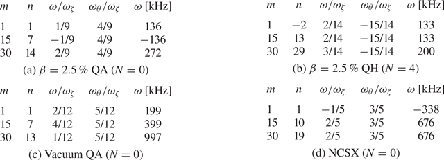
Given a $\omega _{\theta }/\omega _{\zeta } = p/q$ periodic orbit and poloidal mode number $m$, the resonant wave frequency satisfying (3.2) can be expressed as $\omega /\omega _{\zeta } = p'/q$ for some integer $p'$. The toroidal mode number $n$ and the frequency parameter $p'$ are chosen to satisfy the $l = 1$ resonance condition (3.2), given that the $l = \pm 1$ resonance is predicted to give rise to the most substantial radial transport as described in § 3. The value of $n$ is chosen to yield small magnitudes of $|p'|$, corresponding with lower-frequency perturbations. The mode parameters are summarized in table 1.

Table 1. Alfvénic perturbation mode parameters chosen to satisfy the resonance condition (3.2).

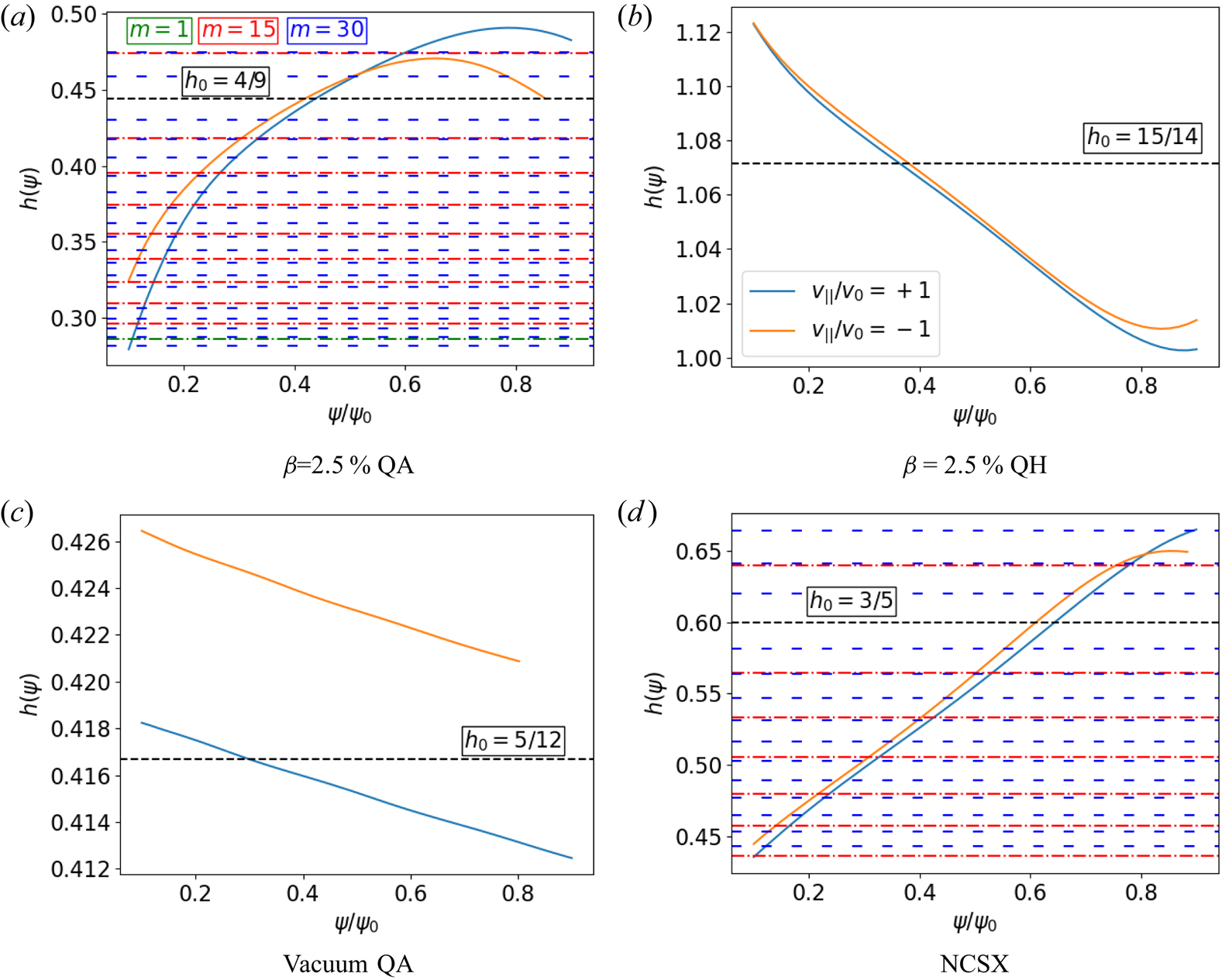
For each configuration, the profile of the effective orbit helicity $h$ (3.5) is shown in figure 2 for co- and counter-passing orbits (blue and orange, respectively). While the helicity profile does not change substantially between co- and counter-passing orbits, the resonance condition (3.5) is modified since the sign and magnitude of $\omega _{\zeta }$ differs. Although the choice of pitch angle will impact the resonance condition, for the following calculations, we focus on co-passing orbits, $v_{\|}/v_0 = +1$. The horizontal black lines in the figures indicate the chosen resonant surface for the co-passing orbits. For the $\beta = 2.5\,\%$ QA and NCSX equilibria, the nearby resonant surfaces corresponding to other values of $l$ are indicated by the coloured horizontal lines. As $m$ increases, the resonance spacing decreases according to (3.6). For the vacuum QA equilibrium, the magnetic shear is very low, see figure 1, and no sideband resonances exist. Although the shear is moderate for the $\beta = 2.5\,\%$ QH equilibrium, sideband resonances are not present due to the factor of $N$ in the resonance spacing expression.

Figure 2. The characteristic orbit helicity, $h = \omega _{\theta }/\omega _{\zeta }$, is computed for co-passing ($v_{\|}/v_0 = +1$, blue) and counter-passing orbits ($v_{\|}/v_0 = -1$, orange). A low-order periodic orbit is selected near the mid-radius, denoted by the horizontal dashed black line. Alfvénic perturbations with several mode numbers $m$ are chosen to resonate with this orbit periodicity. Sideband resonances are excited in the $\beta = 2.5\,\%$ QA and NCSX equilibria due to the angular dependence of the drifts, denoted by the coloured horizontal lines. Because of the increased distance between resonances, no sidebands are excited for in the vacuum QA or $\beta = 2.5\,\%$ QH equilibria for the mode numbers chosen; (a) $\beta = 2.5\,\%$ QA, (b) $\beta = 2.5\,\%$ QH, (c) vacuum QA and (d) NCSX.

5. Kinetic Poincaré plots

Given a magnetic field with exact QS, a kinetic Poincaré plot can be constructed analogously to the case of axisymmetric magnetic fields (Sigmar et al. Reference Sigmar, Hsu, White and Cheng1992). Given a quasisymmetric field $B_0(\psi,\chi =\theta -N\zeta )$ in the absence of a perturbation, the canonical angular momentum

(5.1)\begin{equation} P_{\zeta} = (G + N I) \left(\frac{m v_{\|}}{B_0} + q \alpha \right) + q ( N\psi - \psi_P), \end{equation}

and energy

(5.2)\begin{equation} E = \frac{m v_{\|}^2}{2} + \mu B_0 + q \delta \varPhi, \end{equation}

are conserved. When an Alfvénic perturbation is applied with single mode numbers $n$ and $m$, neither $P_{\zeta }$ nor $E$ are conserved, but a conserved quantity is obtained by moving with the wave frame

(5.3)\begin{equation} \bar{E}_n = (n - N m)E - \omega P_{\zeta}.\end{equation}

Given the velocity-space parameters – $\mu$, $\bar {E}_n$, and $\textrm {sign}(v_{\|})$ – and specification of the position in space and time – $t$, $s$, $\theta$ and $\zeta$ – (5.3) provides a nonlinear equation for $v_{\|}$ (Hsu & Sigmar Reference Hsu and Sigmar1992).

Given the form for the phase factor of the perturbation (2.4), the resulting equations of motion depend on $(s,\chi,\zeta - \bar {\omega }_n t, v_{\|})$, where $\bar {\omega }_n = \omega /(n - N m)$. The resulting motion is generally four-dimensional. If purely passing particles are considered, then ${sign}(v_{\|})$ is fixed, $v_{\|}$ can be computed from the other coordinates as described above, and the resulting motion becomes three-dimensional. For a fixed value of $\bar {E}_n$ and $\mu$, a kinetic Poincaré map $M(s,\chi ) \rightarrow (s',\chi ')$ is constructed by moving with the wave frame to eliminate the time dependence. Guiding-centre trajectories are followed until they intersect a plane of constant $\zeta - \bar {\omega }_nt$. Therefore, the resulting Poincaré section is two-dimensional.

When QS is broken in the equilibrium, $\bar {E}_n$ is no longer precisely conserved. Nonetheless, if the QS errors are sufficiently small, the kinetic Poincaré analysis provides insight into the resulting transport. The non-quasisymmetric modes are artificially suppressed when constructing the kinetic Poincaré plots to aid the analysis. The impact of QS-breaking modes will be assessed in the following section.

In figure 3, kinetic Poincaré plots are displayed for particles with $\textrm {sign}(v_{\|}) = +1$, $\mu = 0$, $E = 3.52$ MeV and Alfvénic perturbations with parameters given in table 1. The amplitude $\hat {\varPhi }$ is chosen such that $\delta \hat {B}^{\psi } = 10^{-3}$ on the $s = 1$ surface. Periodic orbits that satisfy the resonance condition $\varOmega _l = 0$ appear as $n/(m+l)$ periodic orbits in the kinetic Poincaré plots.

Figure 3. Kinetic Poincaré plots are constructed using the mode parameters in table 1 with the perturbation amplitude $\delta \hat {B}^{\psi }= 10^{-3}$. All QS-breaking harmonics of the equilibrium field are artificially suppressed for this analysis; (a) $m = 1$, $\beta = 2.5\,\%$ QA, (b) $m = 15$, $\beta = 2.5\,\%$ QA, (c) $m = 30$, $\beta = 2.5\,\%$ QA, (d) $m = 1$, $\beta = 2.5\,\%$ QH, (e) $m = 15$, $\beta = 2.5\,\%$ QH, ( f) $m = 30$, $\beta = 2.5\,\%$ QH, (g) $m = 1$, vacuum QA, (h) $m = 15$, vacuum QA, (i) $m = 30$, vacuum QA, (j) $m = 1$, NCSX, (k) $m = 15$, NCSX and (l) $m = 30$, NCSX.

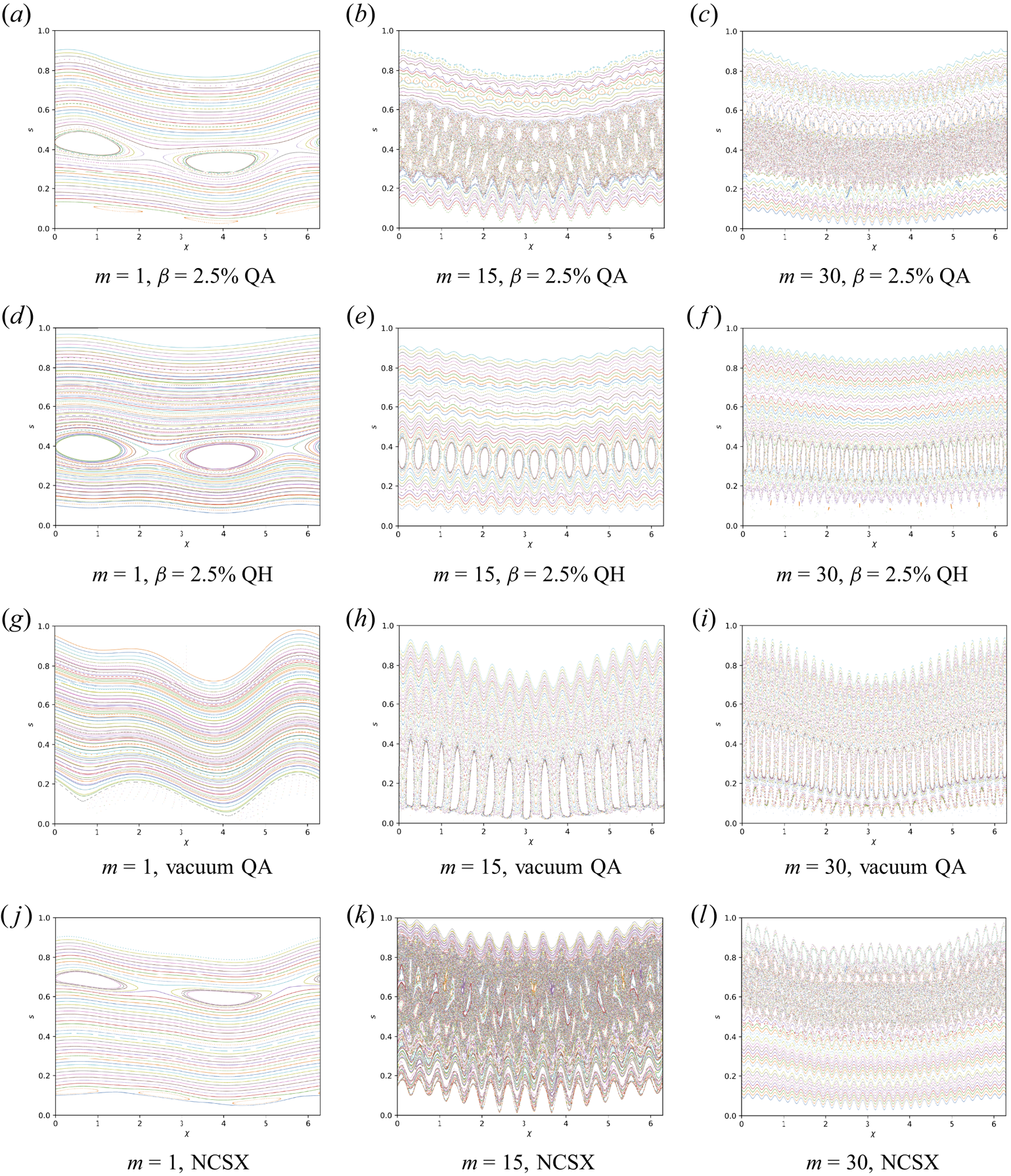
For the NCSX and $\beta = 2.5\,\%$ QA configurations, a clear $l = 1$ island chain is apparent in the presence of the $m = 1$ perturbation. For the vacuum QA equilibrium, the perturbation shifts the orbit helicity slightly, moving the resonance outside the equilibrium due to the low magnetic shear. The resonance reappears by increasing the perturbation frequency by 8 %, see figure 4. In the $\beta = 2.5\,\%$ QA equilibria, in addition to the primary $l = 1$ resonance, the $l = 2$ resonance is apparent near $s = 0.1$. However, the island width is small due to the reduced magnitude of the $J_2(\eta _1)$ coupling parameter. As indicated by the resonance plots, figure 2, none of the other equilibria contain the $m=1$, $l =2$ resonance.

Figure 4. (a) In the presence of the resonant perturbation of amplitude $\delta \hat {B}^{\psi } = 10^{-4}$, the characteristic frequencies $\omega _{\theta }$ and $\omega _{\zeta }$ shift, causing the resonance defined by $\varOmega _l = 0$ to move outside the equilibrium due to the low shear, see figure 3(g). By increasing the mode frequency by 8 %, the resonance re-enters. (b) The kinetic Poincaré plot of amplitude $\delta \hat {B}^{\psi } = 10^{-4}$ with the shifted frequency ($\omega = 2.15$ kHz) reveals the corresponding $l = 1$ island on the shifted resonant surface.

As the mode number increases from $m = 15$ to $m = 30$, the $l = 1$ island width stays roughly the same for the $\beta = 2.5\,\%$ QH configuration, as indicated by the scaling of the island width formula (3.3) and (3.4) for fixed $\delta \hat {B}^{\psi }$. For the vacuum QA configuration, the $l = 1$ resonance reappears for the $m = 15$ and $m = 30$ perturbations, its width being especially wide due to the low magnetic shear of the configuration. For both the vacuum QA and $\beta = 2.5\,\%$ QH configurations with the $m = 15$ and $m = 30$ perturbations, the island chain is wide enough to lead to visible destruction of nearby KAM surfaces and the formation of secondary island chains.

In the $\beta = 2.5\,\%$ QA equilibrium, overlap between the $l = 0$, 1, 2 and 3 resonances is observed with the $m = 15$ perturbation. Substantial island overlap is also observed in the NCSX equilibrium with the $m = 15$ perturbation. In the presence of the $m = 30$ perturbation, strong island overlap is observed in the $\beta = 2.5\,\%$ QA and NCSX equilibria. However, the phase-space volume over which island overlap occurs is narrowed. As seen in figure 2, the resonances become more closely spaced for the $m = 30$ perturbation compared with the $m = 15$ perturbation. However, because the island width scales as $\sqrt {\eta _1^{|l|}}$ with $\eta _1 \ll 1$, island overlap does not occur for the large $|l|$ resonant surfaces. This island width scaling effectively reduces the non-integrable volume as $m$ increases.

The impact of these phase-space features on the resulting transport will be discussed in § 6.

5.1. Impact of QS deviations

We now investigate the impact of the finite QS deviations, quantified in figure 1, on the kinetic Poincaré analysis. When QS deviations are present, the motion of passing particles becomes four-dimensional $(s,\chi,\zeta,t)$, and the Poincaré section becomes three-dimensional, $M(s,\chi,\zeta ) \rightarrow (s',\chi ',\zeta ')$. Nonetheless, we can still visualize the Poincaré map in the $(s,\chi )$ plane to assess the structure of phase space.

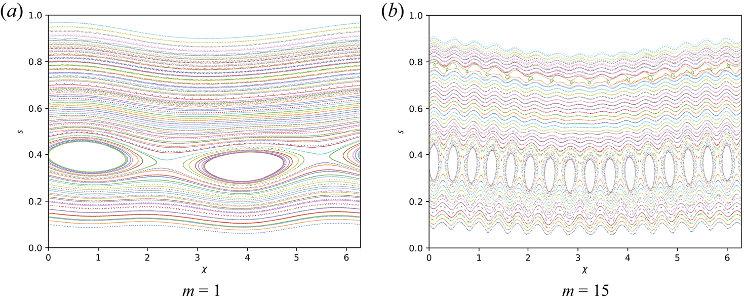
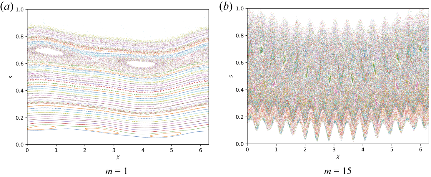
In figures 5 and 6, we show a selection of the kinetic Poincaré plots constructed with the same parameters as those in figure 3, but without the suppression of the QS-breaking modes. For the case of the $\beta = 2.5\,\%$ QH equilibrium, the phase-space structure remains mostly unchanged, with the addition of small-scale mixing. In the case of the NCSX equilibrium, the amplitude of the phase-space mixing is amplified due to the enhanced symmetry breaking. The gross phase-space structure remains mostly unchanged in the presence of the $m = 1$ perturbation. In the presence of the $m = 15$ perturbation, the effective diffusion due to the non-integrability of the orbits destroys many of the remaining KAM surfaces and island chains, leading to a wide region of phase-space chaos. We conclude that most large-scale phase space structure is preserved by adding QS deviations, especially for equilibria close to QS, $f_\textrm {QS} \sim 10^{-3}$. This finding does not quantitatively agree with recent results (White & Duarte Reference White and Duarte2023), indicating substantial diffusive losses in an equilibrium very close to QH ($f_\textrm {QS} \sim 10^{-4}$) with an Alfvénic perturbation as small as $\delta \hat {B}^{\psi } \sim 10^{-6}$.

Figure 5. The $\beta = 2.5\,\%$ QH kinetic Poincaré plots with the same parameters as figure 3, but without the suppression of the QS-breaking modes; (a) $m = 1$ and (b) $m = 15$.

Figure 6. The NCSX kinetic Poincaré plots with the same parameters as figure 3, but without the suppression of the QS-breaking modes; (a) $m = 1$ and (b) $m = 15$.

6. Monte Carlo analysis

To assess the impact of the phase-space structure on the resulting transport, we perform Monte Carlo collisionless guiding-centre tracing simulations. We initialize 5000 particles uniformly in pitch angle and volume for $s \in [0.25, 0.75]$. This initial spatial distribution was chosen to avoid effects related to the coordinate singularity. Particles are followed for $10^{-3}$ seconds or until they are considered lost when they cross through $s = 0$ or $s= 1$.Footnote ¹ Figures 7 and 8 display results of tracing performed with the true equilibria (solid curves, ‘equilibrium’) as well as with the QS-breaking modes artificially filtered out (dashed curves, ‘perfect QS’). Calculations are carried out without Alfvénic perturbations ($\hat {\alpha } = 0$) and for the $m = 1$, 15 and 30 perturbations indicated in table 1.

Figure 7. The loss fraction as a function of time is shown. Monte Carlo tracing is performed in the presence of a $\delta \hat {B}^{\psi } = 10^{-3}$ perturbation with parameters described in table 1. Guiding-centre trajectories of fusion-born alpha particles are followed for $10^{-3}$ seconds or until they cross through $s=0$ or $s=1$. A comparison is made between the actual equilibrium and the equilibrium for which the QS-breaking modes are suppressed, ‘perfect QS’; (a) $\beta = 2.5\,\%$ QA, (b) $\beta = 2.5\,\%$ QH, (c) vacuum QA and (d) NCSX.

Figure 8. Distribution of radial displacement, $|\Delta s|$, between $t=0$ and the final recorded time among Monte Carlo samples for the same calculation presented in figure 7; (a) $\beta = 2.5\,\%$ QA, (b) $\beta = 2.5\,\%$ QH, (c) vacuum QA and (d) NCSX.

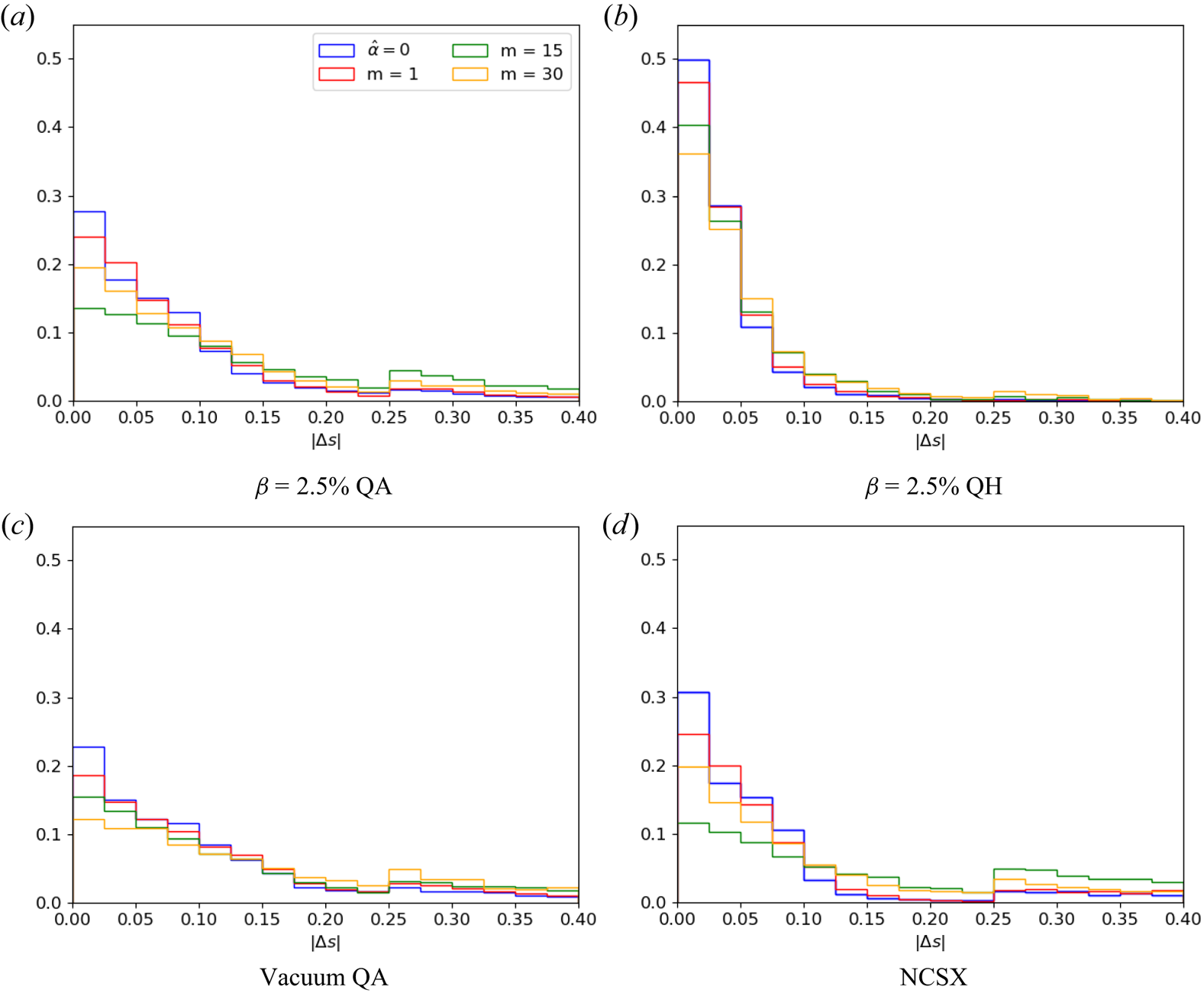
In figure 8, the effective transport is quantified by the distribution of the radial displacement, $|\Delta s|$, between $t = 0$ and the final recorded time (after $10^{-3}$ or when a particle is considered lost). By initializing with a uniform distribution over $s$ in a fixed interval, flattening of the distribution function is not as apparent. On the other hand, the distribution of $|\Delta s|$ allows us to identify the net displacement of trajectories due to phase-space islands or chaos. The double maximum structure reflects the confined trajectories, centred around $|\Delta s| = 0$, and lost trajectories, for which $|\Delta s| \ge 0.25$. The loss fraction as a function of time is also shown in figure 7. A summary of the results is presented in table 2. When comparing the equilibrium and perfect QS cases, we see slight transport enhancement due to QS-breaking modes in the $\beta = 2.5\,\%$ QA and QH and vacuum QA equilibria. The enhancement of transport becomes much more pronounced in the NCSX equilibrium, given its more substantial deviations from QS; see figure 1.

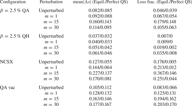
Table 2. Summary of transport properties for Monte Carlo calculations in the presence of Alfvénic perturbations with mode parameters described in table 1 and amplitude $\delta \hat {B}^{\psi } = 10^{-3}$. The mean radial displacement along a trajectory, $\textrm {mean}|\Delta s|$, and total loss fraction after $10^{-3}$ s are compared between the actual equilibrium, ‘equil’, and the equilibrium for which the QS-breaking modes are suppressed, ‘perfect QS’.

In the equilibria that do not exhibit island overlap in figure 3, the vacuum QA and $\beta = 2.5\,\%$ QH equilibria, the total loss fraction increases monotonically with $m$. This result matches the observations in figure 3, which indicate that although the island width remains roughly the same, the destruction of nearby KAM surfaces increases with increasing mode number. On the other hand, in equilibria that exhibit strong resonance overlap in figure 3, NCSX and $\beta = 2.5\,\%$ QA, the transport increases monotonically with $m$ until $m = 15$, then decreases for $m = 30$. This characteristic is explained in terms of the kinetic Poincaré plots in figure 3, which indicate that the effective volume of non-integrability is decreased for $m = 30$ compared with $m = 15$ due to the reduction in island width for large $l$ perturbations.

Overall, the total induced transport is the lowest for the $\beta = 2.5\,\%$ QH configuration, for which the total losses remain less than $10\,\%$ in the presence of the Alfvénic perturbations. The losses are also less prompt for this configuration, with most beginning around $10^{-4}$ seconds, rather than around $10^{-5}$ seconds for the other configurations. This reduction in transport is due to the increased resonance spacing of QH configurations and its increased magnetic shear compared with the vacuum QA equilibria, see figure 1.

6.1. Transition to phase-space chaos

We now study the transition to phase-space chaos and global transport with increasing perturbation amplitude in the $\beta = 2.5\,\%$ QA equilibria. We focus on the $m = 30$ perturbation, given that this is the expected mode number at reactor scales. Kinetic Poincaré plots for co-passing particles resonant with the Alfvénic perturbation are shown in figure 9. The $l = -1$, 0, 1, 2 and 3 islands are visible at the smallest perturbation amplitude, corresponding to $\delta \hat {B}^{\psi } = 3.14 \times 10^{-4}$. As the amplitude is increased to $\delta \hat {B}^{\psi } = 5.58 \times 10^{-4}$, a band of island overlap appears near the resonant surface. The region of destroyed KAM surfaces increases with increasing perturbation amplitude, with only a few remnant islands present at $\delta \hat {B}^{\psi } = 1.76 \times 10^{-3}$.

Figure 9. Kinetic Poincaré plots for co-passing orbits in the $\beta = 2.5\,\%$ QA in the presence of an $m = 30$ perturbation with parameters described in table 1.

Monte Carlo calculations, as described above, are performed for the same Alfvénic perturbations to distinguish the impact of the phase-space structure on transport. The loss fraction as a function of time, initial and final distribution function, and net radial displacement $|\Delta s|$ are shown in figure 10. We note a sudden increase in the loss fraction above $\delta \hat {B}^{\psi } = 5.58\times 10^{-4}$, the value for which island overlap is seen to occur in figure 9. This behaviour is analogous to the observation of critical gradient behaviour on DIII-D, for which the fast-ion transport suddenly becomes stiff above a critical gradient threshold. Similar to our results, the critical gradient behaviour on DIII-D arises due to phase-space stochastization (Collins et al. Reference Collins, Heidbrink, Podestà, White, Kramer, Pace, Petty, Stagner, Van Zeeland and Zhu2017). The initial losses scale approximately as $t^2$, as expected for quasilinear diffusion. As the radial distribution of particles evolves, we see enhanced flattening near the primary resonance surface with increasing perturbation amplitude.

Figure 10. Monte Carlo guiding-centre tracing calculations are performed for the $\beta = 2.5\,\%$ QA configuration in the presence of an $m = 30$ perturbation with parameters described in table 1. The perturbation amplitude is increased to study the impact of island overlap, as illustrated in figure 9, on transport. (a) The loss fraction as a function of time. (b) The distribution of the total radial displacement, $|\Delta s|$, between the initial time and final recorded time. (c) The initial and final radial distribution of particles. (d) The increase in losses of different trajectory classes is plotted as a function of the perturbation amplitudes. The trapped and passing categorization is based on a comparison of the trapping parameter $\lambda = v_{\perp }^2/(v^2B)$ with the maximum field strength on the magnetic surface where a given trajectory is initialized or lost.

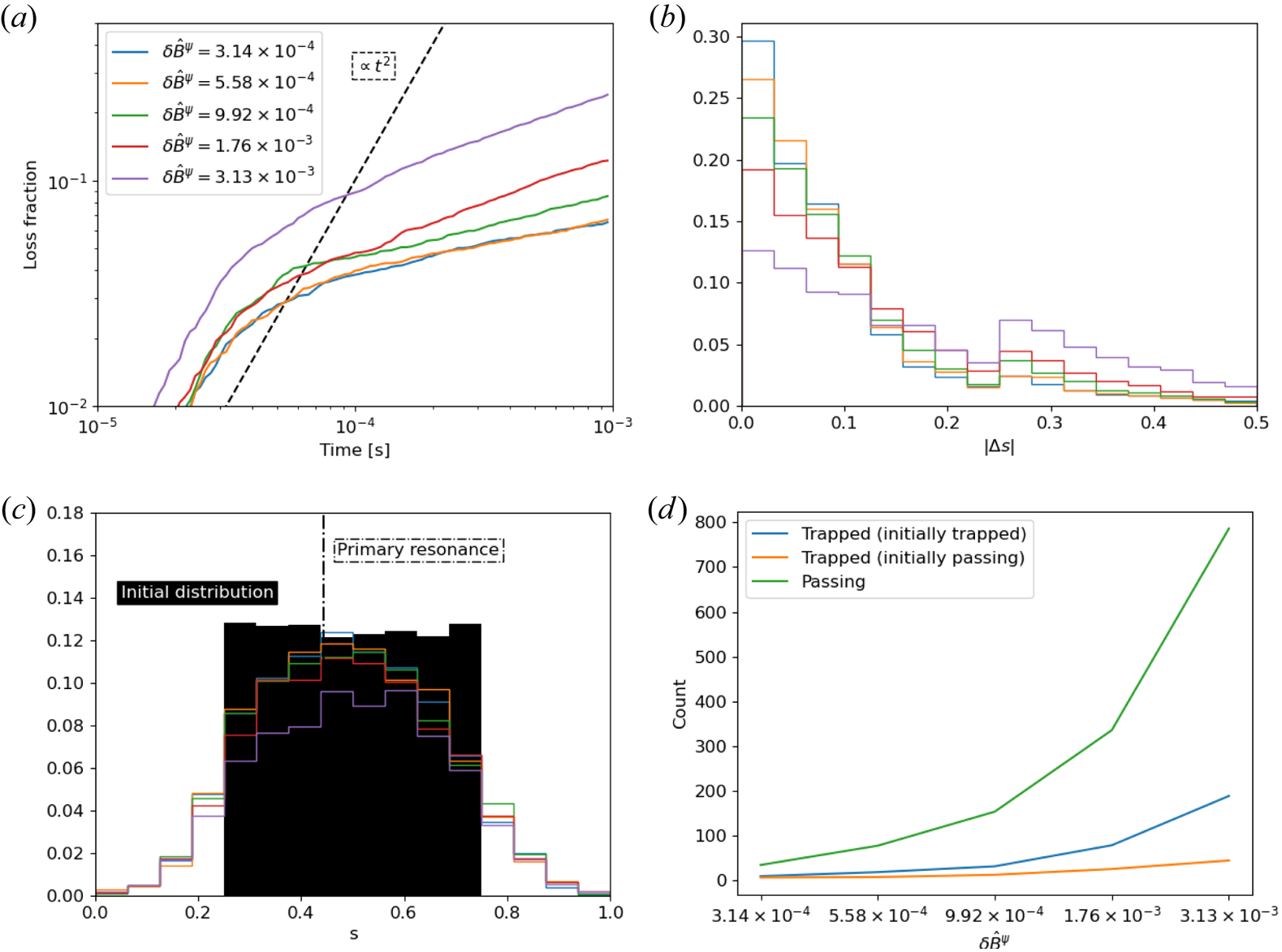
Figure 10(d) displays the trapping state of lost trajectories as a function of the perturbation amplitude. The trapped and passing status at $t = 0$ and the time of loss are assessed by comparing the trapping parameter $\lambda = v_{\perp }^2/(v^2B)$ with the maximum field strength on the initial and final magnetic surfaces. In order to focus on the losses due to the Alfvénic perturbation rather than symmetry-breaking or wide banana orbits, we subtract the count in each category from the losses without an Alfvénic perturbation. As expected, the majority of the loss increase is due to passing orbits. There are additional losses of initially passing orbits that transition to trapped orbits. This loss type can arise from diffusion in the constant of motion space, leading to transformation from a passing orbit to a barely trapped banana orbit with a large radial width (Hsu & Sigmar Reference Hsu and Sigmar1992; Sigmar et al. Reference Sigmar, Hsu, White and Cheng1992). Finally, there are losses of trapped particles that do not originate as passing. Further analysis is needed to understand the responsible loss mechanisms. Overall, we conclude that the kinetic Poincaré analysis provides insight into transport characteristics, even for these configurations with finite deviations from QS.