


1. Introduction
The aerodynamic performance of high-speed vehicles is dominated by boundary layer (BL) physics. Turbulent BLs cause elevated heat transfer and skin friction drag, which are detrimental to the survivability of high-speed aircraft. Thus, from an engineering perspective, extending the laminar flow over the aircraft is beneficial, as it leads to reduced aerodynamic heating and drag, and helps control the weight of the thermal protection systems (Glass Reference Glass2008). The present work aims to understand the mechanisms governing second-mode dominated turbulent transition in hypersonic flows, which is expected to support the engineering of efficient flow control strategies (Chou, Marineau & Smith Reference Chou, Marineau and Smith2023).
1.1. Transition to turbulence in high-speed flows
Transition to turbulence in external flows is typically caused by the BL receiving various types of external disturbances from the free-stream or internal disturbances from surface irregularities on the aircraft body (Reshotko Reference Reshotko1994). This receptivity mechanism is affected by several factors, including the mean flow, vehicle geometry and the amplitude and frequency content of free-stream disturbances. For high-speed flows, the amplification of dominant instabilities can occur through several mechanisms, as depicted by Morkovin, Reshotko & Herbert (Reference Morkovin, Reshotko and Herbert1994), which can be broadly classified into three paths. For low-amplitude disturbances, the BL encourages the growth of specific unstable eigenmodes. For moderate-level disturbances, transient growth may occur, where otherwise stable BL eigenmodes couple due to mutual non-orthogonality and exhibit short-duration algebraic growth $({\sim} \textit{te}^{-t})$
(Reshotko Reference Reshotko2001). Both of these pathways eventually lead to nonlinear mechanisms, i.e. intermodal interactions and sub- or super-harmonic resonances, once a critical amplitude level is surpassed. Finally, for higher-amplitude disturbances, bypass mechanisms dominate the transition process as the modal growth pathway is entirely skipped (Morkovin Reference Morkovin1985).
$({\sim} \textit{te}^{-t})$
(Reshotko Reference Reshotko2001). Both of these pathways eventually lead to nonlinear mechanisms, i.e. intermodal interactions and sub- or super-harmonic resonances, once a critical amplitude level is surpassed. Finally, for higher-amplitude disturbances, bypass mechanisms dominate the transition process as the modal growth pathway is entirely skipped (Morkovin Reference Morkovin1985).
The current work focuses on the first path – the amplification of unstable BL eigenmodes. In free-flight conditions, hypersonic vehicles encounter a low-disturbance free-stream, making the modal growth pathway practically relevant (Schneider Reference Schneider2004) especially on slender geometries at low angles of attack. The modal amplification is the precursor to several types of other multi-mode interactions, which eventually cause transition to turbulence. Such nonlinear interactions can involve K-type resonances (Bake, Meyer & Rist Reference Bake, Meyer and Rist2002), where two oblique waves at equal and opposite angles interact with the dominant mode, or H-type resonances (Herbert Reference Herbert1988), where sub-harmonic oblique modes interact with the primary mode.
1.2. Kinematics and mechanics of hypersonic boundary layer transition
Boundary layer instabilities can be broadly categorised into the following: streamwise-convective or longitudinal, cross-flow, centrifugal (Görtler) or of the attachment-line type (Saric, Reshotko & Arnal Reference Saric, Reshotko and Arnal1998). Streamwise-travelling instabilities are the most prominent in BLs over sharp, slender geometries and at low angles of attack. For higher Mach numbers (Ma $\gt$
5), instability mechanisms are dominated by compressibility effects rather than viscous effects. Consequently, acoustic-like, dilatational instabilities play a more prominent role in high-speed transition under such canonical conditions.
$\gt$
5), instability mechanisms are dominated by compressibility effects rather than viscous effects. Consequently, acoustic-like, dilatational instabilities play a more prominent role in high-speed transition under such canonical conditions.
Lees & Lin (Reference Lees and Lin1946) extended the application of Rayleigh’s incompressible inflection point criterion $(\partial ^2 u_0/\partial y^2=0)$
to the compressible regime, with
$(\partial ^2 u_0/\partial y^2=0)$
to the compressible regime, with $u_0$
denoting the base flow streamwise velocity. They proposed the presence of a generalised inflection point
$u_0$
denoting the base flow streamwise velocity. They proposed the presence of a generalised inflection point $ (\partial /\partial y (\rho _0 \partial u_0/\partial y )=0 )$
as a sufficient condition for the onset of first-mode instabilities, which are dominant in supersonic flows. Here,
$ (\partial /\partial y (\rho _0 \partial u_0/\partial y )=0 )$
as a sufficient condition for the onset of first-mode instabilities, which are dominant in supersonic flows. Here, $\rho_0$
denotes the base flow density. These were observed to be most unstable when oblique, in contrast to the planar Tollmien-Schlichting waves. Lees (Reference Lees1957) then predicted the first modes to be destabilised by wall heating, whereas cooling was predicted to remove the inflection point from the BL and hence, eradicate the first-mode instabilities. Later, Mack (Reference Mack1969) used compressible linear stability theory (LST) to prove the existence of a new family of instability modes, in addition to the first modes. Stability theory suggested that the existence of these modes only requires a region of supersonic flow relative to the disturbance propagation speed, and does not require the presence of a generalised inflection point. These were identified as acoustic-type instabilities trapped within the BL, which are destabilised by wall cooling instead. The fundamental harmonic of this family, the second-mode wave, is most destabilised when planar (or two-dimensional) and is the most dominant instability in the hypersonic transition process under canonical conditions. Our analysis here shows that the generalised inflection point, denoted as
$\rho_0$
denotes the base flow density. These were observed to be most unstable when oblique, in contrast to the planar Tollmien-Schlichting waves. Lees (Reference Lees1957) then predicted the first modes to be destabilised by wall heating, whereas cooling was predicted to remove the inflection point from the BL and hence, eradicate the first-mode instabilities. Later, Mack (Reference Mack1969) used compressible linear stability theory (LST) to prove the existence of a new family of instability modes, in addition to the first modes. Stability theory suggested that the existence of these modes only requires a region of supersonic flow relative to the disturbance propagation speed, and does not require the presence of a generalised inflection point. These were identified as acoustic-type instabilities trapped within the BL, which are destabilised by wall cooling instead. The fundamental harmonic of this family, the second-mode wave, is most destabilised when planar (or two-dimensional) and is the most dominant instability in the hypersonic transition process under canonical conditions. Our analysis here shows that the generalised inflection point, denoted as $y=y_i$
throughout this manuscript, plays an important role in facilitating the trapping of acoustic waves in the BL and initiating second-mode resonance.
$y=y_i$
throughout this manuscript, plays an important role in facilitating the trapping of acoustic waves in the BL and initiating second-mode resonance.
1.2.1. Kinematics of second modes and geometrical acoustics applications
In hypersonic BLs, a region exists where the instability waves propagate supersonically relative to the local mean flow, delineated by the relative sonic line $(y=y_r)$
. The prevailing notion in the literature is that disturbances can establish standing wave-like patterns within this region
$(y=y_r)$
. The prevailing notion in the literature is that disturbances can establish standing wave-like patterns within this region $(y\lt y_r)$
, which acts as an acoustic waveguide trapping a discrete family of modes (Mack Reference Mack1984). To the authors’ knowledge, the first schematic of this process was presented by Morkovin (Reference Morkovin1987, figure 3), which was later redrawn by Saric et al. (Reference Saric, Reshotko and Arnal1998, figure 4). They showed the streamwise-convecting second modes to be trapped underneath
$(y\lt y_r)$
, which acts as an acoustic waveguide trapping a discrete family of modes (Mack Reference Mack1984). To the authors’ knowledge, the first schematic of this process was presented by Morkovin (Reference Morkovin1987, figure 3), which was later redrawn by Saric et al. (Reference Saric, Reshotko and Arnal1998, figure 4). They showed the streamwise-convecting second modes to be trapped underneath $y=y_r$
, which was later highlighted in the schematic shown by Fedorov & Tumin (Reference Fedorov and Tumin2011, figure 2). More recently, Knisely & Zhong (Reference Knisely and Zhong2019, figure 1) provided a detailed schematic of the second-mode instabilities demonstrating them to have a double-deck structure with acoustic waves trapped below the relative sonic line and subsonic rope-like structures at the critical layer above. In the current work, we use the ray-tracing approach to show that acoustic waves get trapped underneath the generalised inflection point
$y=y_r$
, which was later highlighted in the schematic shown by Fedorov & Tumin (Reference Fedorov and Tumin2011, figure 2). More recently, Knisely & Zhong (Reference Knisely and Zhong2019, figure 1) provided a detailed schematic of the second-mode instabilities demonstrating them to have a double-deck structure with acoustic waves trapped below the relative sonic line and subsonic rope-like structures at the critical layer above. In the current work, we use the ray-tracing approach to show that acoustic waves get trapped underneath the generalised inflection point $(y=y_i)$
, rather than the relative sonic line
$(y=y_i)$
, rather than the relative sonic line $(y=y_r)$
.
$(y=y_r)$
.
One of the first works considering geometrical acoustics for wall shear flows was by Kriegsmann & Reiss (Reference Kriegsmann and Reiss1983), where trapped waves were shown to form caustics inside the BL and a method for analysing such caustic fields was presented. Later, Parziale et al. (Reference Parziale, Shepherd and Hornung2015) analysed the second-mode waves using the ray-tracing approach and showed that cooled walls lead to higher wave trapping in the BL. Kuehl (Reference Kuehl2018) suggested the second-mode trapping to be caused by a fluid layer of higher density, and thus higher specific impedance, residing near the BL edge. Inspired by these findings, we use the ray-tracing approach to analyse the kinematics of acoustic wave trapping and its dependency on the wall temperature. We observe the important role played by the generalised inflection line and discuss the competing effects of density and wall-normal velocity gradient in facilitating the trapping.
1.2.2. Mechanics of second-mode instabilities
Kuehl (Reference Kuehl2018) provided an alternative interpretation of the second modes as thermoacoustically driven instabilities, attributing the resonance formation to the presence of an impedance well between the bottom hard wall and the higher-impedance region near the BL edge. Using an inviscid disturbance energy equation, resonance was shown to be sustained through the term $-\partial /\partial y ( \rho _0 T'v' + \rho 'T_0v' )$
, denoted a thermoacoustic Reynolds stress production term in the study. In the manuscript, we denote all laminar base flow quantities as
$-\partial /\partial y ( \rho _0 T'v' + \rho 'T_0v' )$
, denoted a thermoacoustic Reynolds stress production term in the study. In the manuscript, we denote all laminar base flow quantities as $(\cdot)_0$
and fluctuations as
$(\cdot)_0$
and fluctuations as $(\cdot)'$
, with
$(\cdot)'$
, with $p,T,\rho,u,v$
denoting the pressure, temperature, density, streamwise and wall-normal velocities. In our previous study (Roy & Scalo Reference Roy and Scalo2025), we derived a second-order disturbance energy equation without neglecting viscous and thermal diffusion, demonstrating closure of the second-mode energy budgets. The total disturbance energy production is due to the term
$p,T,\rho,u,v$
denoting the pressure, temperature, density, streamwise and wall-normal velocities. In our previous study (Roy & Scalo Reference Roy and Scalo2025), we derived a second-order disturbance energy equation without neglecting viscous and thermal diffusion, demonstrating closure of the second-mode energy budgets. The total disturbance energy production is due to the term $-v's'\partial s_0/\partial y$
with
$-v's'\partial s_0/\partial y$
with $s^\prime =f(T^\prime ,p^\prime ,T_0,p_0)$
denoting the entropy fluctuations. It peaks at the inflection layer
$s^\prime =f(T^\prime ,p^\prime ,T_0,p_0)$
denoting the entropy fluctuations. It peaks at the inflection layer $(y=y_i)$
, which lies below the critical layer
$(y=y_i)$
, which lies below the critical layer $(y_i\lt y_c)$
for cool walls
$(y_i\lt y_c)$
for cool walls $(\Theta=T_w/T_{ad}\lt1)$
, and coincides
$(\Theta=T_w/T_{ad}\lt1)$
, and coincides $(y_i\simeq y_c)$
at near-adiabatic conditions. We also showed that thermoacoustic effects, as defined by the coordinated action of pressure and heat flux fluctuations (Rayleigh Reference Rayleigh1894), act as a sink (and not production) for the disturbance energy.
$(y_i\simeq y_c)$
at near-adiabatic conditions. We also showed that thermoacoustic effects, as defined by the coordinated action of pressure and heat flux fluctuations (Rayleigh Reference Rayleigh1894), act as a sink (and not production) for the disturbance energy.
This prompted us to analyse the relative phasing between fluctuating variables in this work, attempting to understand how disturbance energy is produced or dissipated. A similar study was performed by Tian & Wen (Reference Tian and Wen2021), in which the relative phasing between individual terms in the linearised governing equations was examined for a Mach 6 adiabatic flat plate. However, the dependency on the wall-cooling ratio was not analysed. A term involving the wall-normal velocity fluctuations, $-v'/T_0 \partial T_0/\partial y$
, and a fluctuating conduction term,
$-v'/T_0 \partial T_0/\partial y$
, and a fluctuating conduction term, $\partial ^2 T'/\partial y^2$
, were observed to drive the temporal rate of change of internal energy at the critical layer. Additionally, the near-wall pressure dilatation was found to be driven by the thermal conduction from the wall. They concluded that the second-mode resonance is analogous to the thermoacoustic mechanisms in a Rijke tube. However, the phase analysis conducted in the current study demonstrates that temperature fluctuations initially induce thermal dilatations away from the wall, which then drive near-wall mechanical dilatation through wall-normal flux transport. Thermoacoustic effects, if any, cause absorption of disturbance energy, rather than production.
$\partial ^2 T'/\partial y^2$
, were observed to drive the temporal rate of change of internal energy at the critical layer. Additionally, the near-wall pressure dilatation was found to be driven by the thermal conduction from the wall. They concluded that the second-mode resonance is analogous to the thermoacoustic mechanisms in a Rijke tube. However, the phase analysis conducted in the current study demonstrates that temperature fluctuations initially induce thermal dilatations away from the wall, which then drive near-wall mechanical dilatation through wall-normal flux transport. Thermoacoustic effects, if any, cause absorption of disturbance energy, rather than production.
1.3. Wall-temperature effects on second-mode growth
The effects of wall cooling on supersonic/hypersonic transition have been considered in numerous investigations (Mack Reference Mack1975; Watson Reference Watson1977; Lysenko & Maslov Reference Lysenko and Maslov1984; Blanchard Reference Blanchard1995; Fedorov et al. Reference Fedorov, Soudakov, Egorov, Sidorenko, Gromyko, Bountin, Polivanov and Maslov2015; Oddo et al. Reference Oddo, Hill, Reeder, Chin, Embrador, Komives, Tufts, Borg and Jewell2021), and it is well known that cooled walls destabilise the second modes. To the best of our knowledge, most studies have focused on combining experimental observations with stability analysis, while first-principles-based mechanistic explanations of varying wall temperatures remain limited.
A detailed investigation of the second-mode structure is performed by Unnikrishnan & Gaitonde (Reference Unnikrishnan and Gaitonde2019) using the momentum potential theory by Doak (Reference Doak1989), which decomposes a flow field into the fluid-thermodynamic modes (acoustic, vortical, and thermal modes). The transition in a Mach 6 flat plate was considered, and the effect of surface cooling was studied. The acoustic and thermal components were demonstrated to stay trapped between the wall and the critical layer, while the vorticity, being the dominant component, stayed concentrated near the generalised inflection line. Later, the study was extended to consider a broader range of wall temperatures, as variations in the structure of the second modes were examined (Unnikrishnan & Gaitonde Reference Unnikrishnan and Gaitonde2021), accounting for three-dimensional mechanisms and free-stream radiation by supersonic modes.
The stronger growth rate observed in cooled walls is commonly attributed to the reduction of thermal and hydrodynamic BL heights. In this work, our goal is to provide a description of the mechanics underlying this relationship. Specifically, by employing the disturbance energy framework (Roy & Scalo Reference Roy and Scalo2025), we assess the influence of the wall temperature on the different components of the total disturbance energy, showing where they are generated, and how they are redistributed within the BL via wall-normal fluxes.
1.4. Manuscript outline
The effect of wall temperature on the second-mode structure is the primary focus of this work. Boundary layer-resolved direct numerical simulations (DNS) and LST analysis are performed, offering the supporting dataset for the theoretical investigations.
The manuscript is structured as follows. In § 2, the flow conditions and the DNS set-up are described, and the spectral LST solver is formulated. In § 3, an overview is given of the fundamental questions we consider in this study, and the theoretical tools used to address the questions. Section 4 demonstrates acoustic wave trapping in the BL from two frames of reference, one stationary and another in the frame of the convecting instabilities. Section 5 analyses the eigenstructure of the instabilities via a phase analysis, serving as a precursor to the following sections, where the disturbance energy flux transport and production mechanisms sustaining the second-mode resonance are studied, and the influence of wall temperature is discussed. The findings are summarised in § 6.
Free-stream and wall-temperature conditions considered in this study.

2. Flow conditions and computational set-up
2.1. Base flow definition
The current work considers a transitional hypersonic BL over a slender, sharp-tipped, circular cone of half-angle $3^\circ$
, spanning
$3^\circ$
, spanning $L_x=1.2$
m in the streamwise direction (see figure 1). The cone is exposed to a Mach
$L_x=1.2$
m in the streamwise direction (see figure 1). The cone is exposed to a Mach $6$
flow at
$6$
flow at $0^\circ$
angle of attack with a free-stream unit Reynolds number
$0^\circ$
angle of attack with a free-stream unit Reynolds number $( \textit{Re}_{\infty}=\rho_{\infty} U_{\infty} / \mu_{\infty} )$
of
$( \textit{Re}_{\infty}=\rho_{\infty} U_{\infty} / \mu_{\infty} )$
of $11.3\times 10^6\,\textrm{m}^{-1}$
. The free-stream conditions, given in table 1, are inspired by the experimental set-up (Miller et al. Reference Miller, Jantze, Redmond, Scalo and Jewell2023) at Purdue’s Mach 6 Quiet Tunnel facility, BAM6QT.
$11.3\times 10^6\,\textrm{m}^{-1}$
. The free-stream conditions, given in table 1, are inspired by the experimental set-up (Miller et al. Reference Miller, Jantze, Redmond, Scalo and Jewell2023) at Purdue’s Mach 6 Quiet Tunnel facility, BAM6QT.
Schematic of the flow problem comprising a $\psi _c=3^\circ$
half-angle axisymmetric cone subjected to a hypersonic free-stream flow (see table 1). The table above shows the free-stream Mach number
$\psi _c=3^\circ$
half-angle axisymmetric cone subjected to a hypersonic free-stream flow (see table 1). The table above shows the free-stream Mach number $(M_\infty)$
, unit Reynolds number
$(M_\infty)$
, unit Reynolds number $(Re_\infty)$
, pressure
$(Re_\infty)$
, pressure $(p_\infty)$
, temperature
$(p_\infty)$
, temperature $(T_\infty)$
, density
$(T_\infty)$
, density $(\rho_\infty)$
, velocity
$(\rho_\infty)$
, velocity $(U_\infty)$
and dynamic viscosity
$(U_\infty)$
and dynamic viscosity $(\mu_\infty)$
.
$(\mu_\infty)$
. $(u_e)$
represents the BL edge velocity.
$(u_e)$
represents the BL edge velocity. $\Theta$
is the ratio between the wall temperature
$\Theta$
is the ratio between the wall temperature $(T_w)$
and the adiabatic wall temperature
$(T_w)$
and the adiabatic wall temperature $(T_{ad})$
. In this work,
$(T_{ad})$
. In this work, $T_w$
is varied uniformly above and below
$T_w$
is varied uniformly above and below $T_{ad}$
.
$T_{ad}$
.

The cone wall temperature is isothermal and set by varying the ratio between the wall temperature and the adiabatic (recovery) temperature, $\varTheta =T_w/T_{\textit{ad}}$
. The different ratios considered in this work are shown in figure 2. The recovery temperature for a laminar flow can be estimated as
$\varTheta =T_w/T_{\textit{ad}}$
. The different ratios considered in this work are shown in figure 2. The recovery temperature for a laminar flow can be estimated as $T_{\textit{ad}} = T_e ( 1 + \sqrt {\textit{Pr}} \, (\gamma-1)/2 M_e^2 )$
, with ‘e’ denoting the BL edge quantities (White Reference White2006). In the current work, we assume a Taylor–Maccoll flow over the cone to obtain the BL edge quantities used to calculate the recovery temperature. The resulting wall temperatures are shown in figure 2. Additionally, an adiabatic wall is also considered for comparison with the isothermal
$T_{\textit{ad}} = T_e ( 1 + \sqrt {\textit{Pr}} \, (\gamma-1)/2 M_e^2 )$
, with ‘e’ denoting the BL edge quantities (White Reference White2006). In the current work, we assume a Taylor–Maccoll flow over the cone to obtain the BL edge quantities used to calculate the recovery temperature. The resulting wall temperatures are shown in figure 2. Additionally, an adiabatic wall is also considered for comparison with the isothermal $(\varTheta =1.0)$
case; the former imposes the Neumann conditions on the temperature perturbations
$(\varTheta =1.0)$
case; the former imposes the Neumann conditions on the temperature perturbations $(\partial T'/\partial y=0)$
, while the latter imposes a homogeneous Dirichlet condition
$(\partial T'/\partial y=0)$
, while the latter imposes a homogeneous Dirichlet condition $(T'=0)$
.
$(T'=0)$
.
Base flow profiles at different wall-temperature ratios. The top row shows the temperature and density profiles, while the bottom row shows the velocity profiles along with the speed of sound. The dashed line represents the adiabatic wall results, and the solid lines represent isothermal walls at temperatures $T_w=\varTheta \, T_{\textit{ad}}$
. The values of
$T_w=\varTheta \, T_{\textit{ad}}$
. The values of $\varTheta$
are given in the table above. The profiles are plotted at
$\varTheta$
are given in the table above. The profiles are plotted at $x=0.9$
m (see figure 1).
$x=0.9$
m (see figure 1).

Figure 2 shows the temperature, streamwise velocity, density and sonic speed profiles of the laminar BL, along with the first and second derivatives of the temperature and velocity. The temperature gradient at the wall is positive, zero and negative for the cooled, adiabatic and heated wall cases, respectively. The magnitude of the velocity and temperature gradients at the wall is higher for colder walls than for hotter walls, resulting in significant thermal loading at the wall, as depicted by the highly negative value of $\partial ^2 T_0/\partial y^2$
at the wall. For sufficiently cold walls, the density profiles reveal a lighter fluid region trapped between two denser fluid regions at the wall and at the BL edge. These features of the mean flow profiles play a crucial role in controlling the second-mode growth, as examined in this work.
$\partial ^2 T_0/\partial y^2$
at the wall. For sufficiently cold walls, the density profiles reveal a lighter fluid region trapped between two denser fluid regions at the wall and at the BL edge. These features of the mean flow profiles play a crucial role in controlling the second-mode growth, as examined in this work.
2.2. Governing equations
The hypersonic BL is simulated by numerically solving the fully compressible Navier–Stokes equations, which in index notation, read
 \begin{align} \frac {\partial \rho }{\partial t} + \frac {\partial }{\partial x_{\kern-1pt j}} \left ( \rho u_{\kern-1pt j} \right ) = 0, \\[-28pt] \nonumber \end{align}
 \begin{align} \frac {\partial \left ( \rho u_i \right )}{\partial t} + \frac {\partial }{\partial x_{\kern-1pt j}} \left ( \rho u_i u_{\kern-1pt j} + p\delta _{\textit{ij}} - \tau _{\textit{ji}} \right ) = 0, \\[-28pt] \nonumber \end{align}
 \begin{align} \frac {\partial \left ( \rho E \right )}{\partial t} + \frac {\partial \left ( \rho u_{\kern-1pt j} E \right )}{\partial x_{\kern-1pt j}} = \frac {\partial }{\partial x_{\kern-1pt j}} \left ( \frac {\mu C_p}{\textit{Pr}} \frac {\partial T}{\partial x_{\kern-1pt j}} \right ) -\frac {\partial \left (u_i p\delta _{\textit{ij}}\right )}{\partial x_{\kern-1pt j}} + \frac {\partial \left (u_i \tau _{\textit{ji}} \right )}{\partial x_{\kern-1pt j}} , \\[2pt] \nonumber \end{align}
where $(x_1,x_2,x_3) = (X,Y,Z)$
denotes the Cartesian system. The system
$(x_1,x_2,x_3) = (X,Y,Z)$
denotes the Cartesian system. The system $(x,y)$
denotes the two-dimensional, BL-attached coordinate system (see figure 3). The effect of gravity is ignored, and other source terms are not present in the problem considered. The total energy (per unit mass),
$(x,y)$
denotes the two-dimensional, BL-attached coordinate system (see figure 3). The effect of gravity is ignored, and other source terms are not present in the problem considered. The total energy (per unit mass), $E$
, is the sum of specific internal energy,
$E$
, is the sum of specific internal energy, $e$
, and specific kinetic energy,
$e$
, and specific kinetic energy, $E=e + V^2/2$
, where
$E=e + V^2/2$
, where $V=u_{\kern-1pt j}u_{\kern-1pt j}$
. The viscous stress tensor
$V=u_{\kern-1pt j}u_{\kern-1pt j}$
. The viscous stress tensor $\tau _{\textit{ji}}$
is given as
$\tau _{\textit{ji}}$
is given as $\mu ( \partial u_{\kern-1pt j}/\partial x_i + \partial u_i/\partial x_{\kern-1pt j} ) + \lambda (\partial u_k/\partial x_k) \delta _{\textit{ij}}$
, where
$\mu ( \partial u_{\kern-1pt j}/\partial x_i + \partial u_i/\partial x_{\kern-1pt j} ) + \lambda (\partial u_k/\partial x_k) \delta _{\textit{ij}}$
, where $\delta _{\textit{ij}}$
is the Kronecker delta and
$\delta _{\textit{ij}}$
is the Kronecker delta and $\lambda =-2/3\mu$
is used assuming that bulk viscosity
$\lambda =-2/3\mu$
is used assuming that bulk viscosity $\mu _b=0$
(Stokes’ hypothesis). The above equations are written in terms of the total fluid variables, which can be decomposed into a laminar mean state and a perturbation about the mean, as
$\mu _b=0$
(Stokes’ hypothesis). The above equations are written in terms of the total fluid variables, which can be decomposed into a laminar mean state and a perturbation about the mean, as $(.)=(.)_0+(.)'$
. Hereafter, we use these notations to denote the mean and the perturbation components.
$(.)=(.)_0+(.)'$
. Hereafter, we use these notations to denote the mean and the perturbation components.
The stagnation temperature of the chosen flow remains much below the ionisation point of air. Thus, air has been modelled as an ideal, calorically perfect gas following $p=\rho \textit{RT}$
, with a specific gas constant,
$p=\rho \textit{RT}$
, with a specific gas constant, $R=287$
J kg
$R=287$
J kg $^{-1}$
K
$^{-1}$
K $^{-1}$
, specific heat ratio,
$^{-1}$
, specific heat ratio, $\gamma =1.4$
, specific heat capacity,
$\gamma =1.4$
, specific heat capacity, $C_p=\gamma R / (\gamma - 1)$
, and Prandtl number,
$C_p=\gamma R / (\gamma - 1)$
, and Prandtl number, $ \textit{Pr}=0.707$
. Viscosity is modelled as a function of temperature, using the low-temperature correction on Sutherland’s law, as given by Mack (Reference Mack1965).
$ \textit{Pr}=0.707$
. Viscosity is modelled as a function of temperature, using the low-temperature correction on Sutherland’s law, as given by Mack (Reference Mack1965).
2.3. Set-up for axisymmetric direct numerical simulations
The numerical simulations are performed using CFDSU, a Fortran-based finite difference solver originally developed by Nagarajan, Lele & Ferziger (Reference Nagarajan, Lele and Ferziger2003) that has been consistently developed and maintained at Purdue University. The solver has been used for various types of flow applications previously, including Large Eddy Simulation modelling (Chen & Scalo Reference Chen and Scalo2021), vortex dynamics (Chapelier, Wasistho & Scalo Reference Chapelier, Wasistho and Scalo2018; Zhao & Scalo Reference Zhao and Scalo2021), hypersonic transitional (Sousa et al. Reference Sousa, Wartemann, Wagner and Scalo2024) and turbulent flows (Toki et al. Reference Toki, Sousa, Chen and Scalo2024). CFDSU solves the Navier–Stokes equations in a structured curvilinear grid using the staggered arrangement. Several time integration and spatial discretisation schemes are available in CFDSU. For the present purposes, a low-storage, fourth-order accurate, 6-stage Runge–Kutta scheme (Allampalli et al. Reference Allampalli, Hixon, Nallasamy and Sawyer2009) and the compact sixth-order scheme by Visbal & Gaitonde (Reference Visbal and Gaitonde2002) are used for time integration and spatial discretisation, respectively. This numerical strategy is expected to achieve spectral-like numerical accuracy with low numerical dissipation, which is required for simulating a transitional hypersonic BL.
Summary of the computational set-up for high-order DNS calculations: (a) a low-order precursor run resolving the shock $(\psi _s=9.808^\circ )$
is used to drive (b) embedded high-order DNS on a near-wall, BL-focused domain. A grid-independent pseudorandom noise is imposed at the wall to trigger turbulent transition in the embedded DNS calculations.
$(\psi _s=9.808^\circ )$
is used to drive (b) embedded high-order DNS on a near-wall, BL-focused domain. A grid-independent pseudorandom noise is imposed at the wall to trigger turbulent transition in the embedded DNS calculations.

It is known that the second modes, which are the dominant instabilities for hypersonic transition, are predominantly two-dimensional in nature. Over axisymmetric bodies, they evolve into azimuthal streaks due to mean flow distortion (Chynoweth et al. Reference Chynoweth, Schneider, Hader, Fasel, Batista, Kuehl, Juliano and Wheaton2019) before the eventual three-dimensional turbulent breakdown. The present investigation focuses on the initial modal amplification stage of the transition process, which is the primary destabilisation pathway for BL flow under low free-stream disturbance levels. For these purposes, axisymmetric DNS is deemed sufficient. The DNS set-up used here comprises the following three steps, taking special care in removing spurious numerical artefacts:
-
(i) Low-order precursor – the DNS solver requires an initial laminar base flow to start the simulations. For this, we combine the Taylor–Maccoll (TM) inviscid flow approximation for the region between the shock and the BL edge, and the compressible Blasius similarity approximation for the near-wall, BL viscous flow. This is imposed on the left boundary of the computational domain (see figure 3 a). A low-order calculation, using a second-order finite differencing scheme with a centralised stencil, then propagates the TM + Blasius solution downstream. This allows the pressure adjustments that occur due to precision mismatch between the TM + Blasius Ordinary Differential Equation (ODE) solver and the low-order DNS to wash off, leading to a more accurate laminar base flow. The precursor simulations are performed on a larger computational domain, resolving the shock. The shock was captured using the Localised-artificial diffusivity method by Kawai & Lele (Reference Kawai and Lele2008), relying on the addition of artificial bulk and dynamic viscosity, and conductivity to the governing equations. Care is taken not to add artificial diffusion near the wall to avoid contaminating the BL solution.
-
(ii) High-order stationary base flow – the statistically stationary laminar flow from the low-order precursor run is then used to initialise BL-focused high-order DNS calculations (see figure 3 b) that use a quasi-spectral sixth-order scheme in a compact stencil (Visbal & Gaitonde (Reference Visbal and Gaitonde2002)). Additionally, we use a sixth-order Pade filter with filter coefficient $\alpha =0.49$
to remove spurious high-frequency wavenumbers. As the numerical transients wash off downstream, the thus-obtained stationary flow represents the quiet laminar hypersonic flow solution over the cone, which is used as the base flow for our LST analysis.
$\alpha =0.49$
to remove spurious high-frequency wavenumbers. As the numerical transients wash off downstream, the thus-obtained stationary flow represents the quiet laminar hypersonic flow solution over the cone, which is used as the base flow for our LST analysis. -
(iii) Artificial noise – a controlled perturbation is required to initiate transitional waves in an otherwise numerically quiet laminar flow. Its spectral signature is modulated so that the artificial forcing is independent of the computational grid used. This is achieved by filtering a discretely sampled field in the Legendre spectral space to remove features above a chosen cutoff wavenumber. The analytical form of the noise, resulting from the spectral projection, ensures that the discrete sampling at the grid points remains consistent across different levels of grid refinement. The imposed velocity fluctuations at the wall are given as
(2.2)where
\begin{align} v'_w (x, y=0, t) = A_0 \sum _{m=0}^{m_f-1} a(f_m) \textrm{Re} \left ( \bar {\phi }_m(x) e^{-2\pi i f_m t} \right )\!, \end{align}
$A_0$
is a dimensional coefficient controlling the overall signal amplitude,
$a(f_m)\in [-1,1]$
is a frequency-dependent normalised amplitude modulation and
$\bar {\phi }_m(x)\in [-1,1]$
is the spatially filtered one-dimensional field. A total of
$m_f$
such fields, one for each discrete frequency,
$f_m$
, are imposed simultaneously. The forcing has been applied over the time span
$t \in [0,n_{c}/f_0 ]$
in the simulations, where
$f_0$
is the lowest frequency considered and
$n_{c}$
represents a certain number of periodic cycles. The forcing is introduced in the region
$x\in [0.255,0.301]$
m for all cases considered in this work. Discrete frequencies in the range of
$f_m\in [60{-}200]$
kHz at intervals of
$10$
kHz are used. In all the DNS runs, the forcing is applied over
$n_c=5$
cycles of the lowest frequency,
$60$
kHz, starting from
$t=0$
, with the amplitude
$A_0= (10^{-3},\,10^{-2} )$
(m s−1), which corresponds to
$p^\prime _w/p_\infty =5.5\times (10^{-6},\,10^{-5} )$
. For the temporal spectra modulation function,
$a(f_m)$
, an inverse-frequency dependence (pink noise) is used, mimicking the free-stream noise present in supersonic/hypersonic wind tunnels (Duan et al. Reference Duan2019). Further details regarding the implementation of the forcing function and the rationale behind the choice for
$n_c$
are discussed in Roy & Scalo (Reference Roy and Scalo2025).


2.4. Laguerre–Galerkin spectral linear stability theory
A companion linear stability analysis is performed to support the DNS results and complement the phase relationship analysis between the flow variables. Linear stability theory involves representing the fluctuating flow variables as normal modes, which, upon plugging into the linearised governing equations, form an eigenvalue problem. For the LST analysis, the fluctuating modes are assumed to be locally parallel, meaning that the mode shapes are functions of the wall-normal coordinate only. LST, however, does not account for the inter-modal interactions and non-parallel effects, i.e. the effect of the BL growth. The non-parallel effects are more prominent near the leading edge, where the BL height increases rapidly. This study concentrates on the linear amplification stage away from the leading edge, where the non-parallel effects are not significant. In fact, excellent agreement is shown between DNS and the present LST formulation by Roy & Scalo (Reference Roy and Scalo2025) for the current free-stream flow conditions at a wall temperature of 300 K $(\varTheta \approx 0.85)$
.
$(\varTheta \approx 0.85)$
.
Considering the two-dimensional, BL-attached coordinate system $(x,y)$
(see figure 3), the ansatz used is
$(x,y)$
(see figure 3), the ansatz used is $\psi '=\hat {\psi }(y)e^{i(\alpha x-\omega t)}$
, where
$\psi '=\hat {\psi }(y)e^{i(\alpha x-\omega t)}$
, where $\psi '=(p',T',u',v')$
represents the fluctuating variables. The density perturbation terms in the governing equations can be recast in terms of
$\psi '=(p',T',u',v')$
represents the fluctuating variables. The density perturbation terms in the governing equations can be recast in terms of $p'$
and
$p'$
and $T'$
using the equation of state. When the governing (2.1) are decomposed into mean and fluctuating states and the above ansatz is substituted in, the resulting system of equations takes the following form:
$T'$
using the equation of state. When the governing (2.1) are decomposed into mean and fluctuating states and the above ansatz is substituted in, the resulting system of equations takes the following form:
 \begin{align} L\frac {{\rm d}^2 \hat {\psi }}{{\rm d}y^2} + M\frac {{\rm d} \hat {\psi }}{{\rm d}y} + N \hat {\psi } = 0, \end{align}
where $L, M$
and
$L, M$
and $N$
are matrices dependent on the base flow
$N$
are matrices dependent on the base flow $\psi _0(x,y)$
, the wavenumber
$\psi _0(x,y)$
, the wavenumber $(\alpha )$
and the angular frequency
$(\alpha )$
and the angular frequency $(\omega )$
. We note that here we are considering a local one-dimensional linear stability problem, where (2.3) represents a separate stability problem to be solved for each
$(\omega )$
. We note that here we are considering a local one-dimensional linear stability problem, where (2.3) represents a separate stability problem to be solved for each $x$
location.
$x$
location.
The wall-normal derivatives can be discretised by any finite differencing schemes, as outlined by Malik (Reference Malik1990). When discretised on $n$
points in
$n$
points in $y$
, the
$y$
, the $L,M,N$
matrices have the shape
$L,M,N$
matrices have the shape $4n\times 4n$
, representing the four conservation equations for mass, x- and y-momenta and energy. Here, a spectral Galerkin approach is used for the spatial discretisation (Shen, Tang & Wang Reference Shen, Tang and Wang2011), in which the mode shapes are expanded using a suitable spectral basis as
$4n\times 4n$
, representing the four conservation equations for mass, x- and y-momenta and energy. Here, a spectral Galerkin approach is used for the spatial discretisation (Shen, Tang & Wang Reference Shen, Tang and Wang2011), in which the mode shapes are expanded using a suitable spectral basis as $\hat {\psi }(y)=\sum _{k=0}^n \tilde {\psi }_k\phi _k(y)$
. Here,
$\hat {\psi }(y)=\sum _{k=0}^n \tilde {\psi }_k\phi _k(y)$
. Here, $\phi _k$
represents mutually orthogonal, globally smooth basis functions and
$\phi _k$
represents mutually orthogonal, globally smooth basis functions and $\tilde {\psi }_k$
the associated weights. The global nature of spectral methods imparts a much superior accuracy than local discretisation schemes. The Galerkin approach to solve for the unknown weights
$\tilde {\psi }_k$
the associated weights. The global nature of spectral methods imparts a much superior accuracy than local discretisation schemes. The Galerkin approach to solve for the unknown weights $\tilde {\psi }_k$
involves taking an inner product of (2.3) on the spectral space spanned by the basis functions outlined in the following section. The mutual orthogonality of the functions allows the inner product operation to form separate equations for the unknown weights, which can be solved for. The resulting equation from this operation, representing the projection of (2.3) on the spectral space, reads
$\tilde {\psi }_k$
involves taking an inner product of (2.3) on the spectral space spanned by the basis functions outlined in the following section. The mutual orthogonality of the functions allows the inner product operation to form separate equations for the unknown weights, which can be solved for. The resulting equation from this operation, representing the projection of (2.3) on the spectral space, reads
 \begin{align} \sum _{k=0}^{n-1} \left [ \big ( L D^2\phi _k, \phi _j \big )_w + \left ( \textit{MD}\phi _k, \phi _j \right )_w + \big ( N \phi _k, \phi _j \big )_w \right ]\tilde {\psi }_k = 0, \quad \forall \,0 \leqslant j \leqslant n, \end{align}
where $D$
denotes the derivative operator
$D$
denotes the derivative operator $d/dy$
, and
$d/dy$
, and $(.,.)_w$
denotes the weighted inner product of two functions. At this point, two types of eigenvalue problems can be formulated – spatial or temporal – depending on whether
$(.,.)_w$
denotes the weighted inner product of two functions. At this point, two types of eigenvalue problems can be formulated – spatial or temporal – depending on whether $\omega$
or
$\omega$
or $\alpha$
is considered real, respectively. For the second-mode waves, which are convective instabilities, the spatial and temporal theory results are interrelated (Gaster & Grant Reference Gaster and Grant1975), and solving one or the other imparts the relevant BL stability characteristics. In the present study, the spatial stability eigenvalue problem is solved, which involves finding the complex eigenvalue
$\alpha$
is considered real, respectively. For the second-mode waves, which are convective instabilities, the spatial and temporal theory results are interrelated (Gaster & Grant Reference Gaster and Grant1975), and solving one or the other imparts the relevant BL stability characteristics. In the present study, the spatial stability eigenvalue problem is solved, which involves finding the complex eigenvalue $\alpha =\alpha _r+i\alpha _i$
for each real frequency
$\alpha =\alpha _r+i\alpha _i$
for each real frequency $\omega$
. As per the ansatz convention used,
$\omega$
. As per the ansatz convention used, $-\alpha _i$
represents the amplification rate of the modes.
$-\alpha _i$
represents the amplification rate of the modes.
It is to be noted that the spatial problem involves solving an equation of the form $\sum _{k=0}^{n-1} (\alpha ^2 M + \alpha C + K)\tilde {\psi }_k=0$
, which results in a quadratic eigenvalue problem for
$\sum _{k=0}^{n-1} (\alpha ^2 M + \alpha C + K)\tilde {\psi }_k=0$
, which results in a quadratic eigenvalue problem for $\alpha$
. One way to solve this problem is by extending the definition of
$\alpha$
. One way to solve this problem is by extending the definition of $\tilde {\psi }_k$
to
$\tilde {\psi }_k$
to $ ( \tilde {\psi }_k, \alpha \tilde {\psi }_k )^T$
so that a generalised eigenvalue problem is recovered of the form,
$ ( \tilde {\psi }_k, \alpha \tilde {\psi }_k )^T$
so that a generalised eigenvalue problem is recovered of the form, $\alpha B\boldsymbol{v}=A\boldsymbol{v}$
. Upon solving, the eigenvalues
$\alpha B\boldsymbol{v}=A\boldsymbol{v}$
. Upon solving, the eigenvalues $\alpha$
will provide the exponential growth rates
$\alpha$
will provide the exponential growth rates $(-\alpha _i)$
and wavenumbers
$(-\alpha _i)$
and wavenumbers $(\alpha _r)$
. The eigenvectors
$(\alpha _r)$
. The eigenvectors $\boldsymbol{v}=(\tilde {p}, \tilde {T}, \tilde {u}, \tilde {v})$
, representing the weights of the spectral expansion, ultimately define the wall-normal mode shapes
$\boldsymbol{v}=(\tilde {p}, \tilde {T}, \tilde {u}, \tilde {v})$
, representing the weights of the spectral expansion, ultimately define the wall-normal mode shapes $\hat {\psi }(y)$
.
$\hat {\psi }(y)$
.
2.4.1. Choice of spectral basis
The present work focuses on the stability of a semi-infinite flow problem, for which the generalised Laguerre functions are a suitable expansion basis (Shen et al. Reference Shen, Tang and Wang2011). Perturbations in the flow quantities due to the presence of the instability modes are expected to decay away from the BL, and by definition, the Laguerre functions decay exponentially in the positive real axis $[0,\infty )$
, rendering them a natural choice for semi-infinite flows. The nodes and weights are computed using the Laguerre–Gauss–Radau quadrature, and the base flow variables are interpolated at the quadrature nodes using a piecewise cubic spline interpolation. The unbounded domain is suitably scaled by a factor to increase the number of nodes in the BL (see Shen et al. Reference Shen, Tang and Wang2011, pp. 278–281), improving the numerical accuracy.
$[0,\infty )$
, rendering them a natural choice for semi-infinite flows. The nodes and weights are computed using the Laguerre–Gauss–Radau quadrature, and the base flow variables are interpolated at the quadrature nodes using a piecewise cubic spline interpolation. The unbounded domain is suitably scaled by a factor to increase the number of nodes in the BL (see Shen et al. Reference Shen, Tang and Wang2011, pp. 278–281), improving the numerical accuracy.
The spectral basis used for expanding the fluctuation variables is modified so that the homogeneous Dirichlet boundary conditions (BCs) are implicitly satisfied at the wall. The BCs there are no slip $(u^\prime =0)$
, no penetration
$(u^\prime =0)$
, no penetration $(v^\prime =0)$
and isothermal
$(v^\prime =0)$
and isothermal $(T^\prime =0)$
. The algebraic modification required for this is given as
$(T^\prime =0)$
. The algebraic modification required for this is given as
 \begin{align} \phi _k(y) = \mathcal{L}_k(y) - \mathcal{L}_{k+1}(y), \quad \forall 0 \leqslant k \leqslant n-1, \end{align}
where $\mathcal{L}_k(y)$
denotes the
$\mathcal{L}_k(y)$
denotes the $k$
th generalised Laguerre function. For adiabatic walls, a Neumann BC is to be imposed at the wall on temperature fluctuations,
$k$
th generalised Laguerre function. For adiabatic walls, a Neumann BC is to be imposed at the wall on temperature fluctuations, $(\partial T'/\partial y)_w=0$
. This requires a different algebraic modification to the expansion basis (Shen Reference Shen2000, p. 1126), given as
$(\partial T'/\partial y)_w=0$
. This requires a different algebraic modification to the expansion basis (Shen Reference Shen2000, p. 1126), given as
 \begin{align} \phi _k(y) = \mathcal{L}_k(y) - \frac {2k+1}{2k+3}\mathcal{L}_{k+1}(y), \quad \forall 0 \leqslant k \leqslant n-1. \end{align}
For the other fluctuation variables, (2.5) is used. For $p^\prime$
, the Laguerre basis
$p^\prime$
, the Laguerre basis $(\mathcal{L}_k)$
can be used without modifications, as it is not required to satisfy any BC.
$(\mathcal{L}_k)$
can be used without modifications, as it is not required to satisfy any BC.
3. Theoretical framework and research objectives
This manuscript investigates the fundamental mechanisms governing hypersonic transition in the canonical set-up shown in figure 4(a). The most unstable eigenmodes in this case are the second modes, first predicted by Mack (Reference Mack1969). The second-mode waves are not sustained by viscous mechanisms and behave as inviscid-type waves trapped underneath the BL, forming the characteristic rope-wave structures observed in several experiments (Demetriades Reference Demetriades1974; Stetson & Kimmel Reference Stetson and Kimmel1993). The second-mode mechanics are heavily dependent on the wall temperature, as they are destabilised more over colder walls. This work aims to understand the fundamental mechanisms underlying this wall-temperature dependence.
This study aims to answer the following specific questions:
-
(i) Where are second-mode waves trapped in the BL, and how are they formed?
-
(ii) What fluid dynamic mechanisms cause the production of disturbance energy and its redistribution within the BL?
-
(iii) How does wall temperature influence the production and distribution of energy?
Schematic supporting the formulation of the theoretical questions being tackled in this work: (a) observational window for evaluation of the wavepacket energy during its convective evolution; (b) double-deck structure of second-mode waves with rope-like structures carrying disturbance energy near the critical layer and trapped acoustic modes accumulating energy near the wall; (c) quiver plot of the fluctuating velocity vector field overlaid onto fluctuating pressure field and fluctuating temperature field, indicative of the production mechanisms sustaining second-mode resonance.

We use acoustic ray tracing to examine the trapping of waves in the BL by studying the motion of individual acoustic rays making up a wavefront. A novel disturbance energy equation (Roy & Scalo Reference Roy and Scalo2025) is used to gain insights into the energy production mechanisms fuelling instability growth. We use the flow-field data from DNS (figure 4 c) and LST (figure 4 b) to analyse the phase relationships between fluctuating flow variables and characterise what causes production and dissipation of disturbance energy.
3.1. Disturbance energy equation
To investigate the mechanisms of second-mode growth, we use a second-order closure for the perturbation energy budget, derived in an earlier work (Roy & Scalo Reference Roy and Scalo2025). The equation, inspired by the works of Myers (Reference Myers1991), describes the evolution of perturbation energy in the following conservation form:
 \begin{align} \frac {\partial E_2}{\partial t} + \frac {\partial I_{2j}}{\partial x_{\kern-1pt j}} = D_2, \end{align}
where the second-order disturbance energy term, $E_2$
, representing the energy content of a disturbance wave packet, is given as
$E_2$
, representing the energy content of a disturbance wave packet, is given as
 \begin{align} E_2 = \underbrace {\frac {1}{2} \frac {\rho _0 T_0}{C_p}s'^2}_{i} + \underbrace {\rho ' u_{0i}u_i'}_{\textit{ii}} + \underbrace {\frac {1}{2} \rho _0 u_i'^2}_{\textit{iii}}+ \underbrace {\frac {1}{2}\frac {p'^2}{\gamma p_0}}_{\textit{iv}}. \end{align}
The above expression represents the disturbance’s contribution to the total instantaneous energy of a fluid element. In (3.2), term $(i)$
denotes the thermal potential energy stored in the temperature/entropy hot spots, while terms
$(i)$
denotes the thermal potential energy stored in the temperature/entropy hot spots, while terms $(\textit{ii})$
and
$(\textit{ii})$
and $(\textit{iii})$
collectively represent the kinetic energy of the perturbation. Since term
$(\textit{iii})$
collectively represent the kinetic energy of the perturbation. Since term $(\textit{ii})$
arises due to the non-zero base flow, it will be referred to as the mean flow energy term throughout this work to differentiate it from term
$(\textit{ii})$
arises due to the non-zero base flow, it will be referred to as the mean flow energy term throughout this work to differentiate it from term $(\textit{iii})$
, which will be denoted simply as the disturbance kinetic energy. Finally, term
$(\textit{iii})$
, which will be denoted simply as the disturbance kinetic energy. Finally, term $(\textit{iv})$
quantifies the acoustic or mechanical potential energy resulting from compression and rarefaction work.
$(\textit{iv})$
quantifies the acoustic or mechanical potential energy resulting from compression and rarefaction work.
The energy flux term, $I_{2j}$
, quantifies the flux of each of the above-mentioned disturbance energy components and is given as
$I_{2j}$
, quantifies the flux of each of the above-mentioned disturbance energy components and is given as
 \begin{align} I_{2j} = \underbrace {\frac {1}{2} \frac {\rho _0 T_0}{C_p}s'^2 u_{0j}}_{i} + \underbrace {\rho _0 u_{0i}u_i' \left ( u_{\kern-1pt j}' + \frac {\rho ' u_{0j}}{\rho _0} \right )}_{ii} + \underbrace {\frac {1}{2} \rho _0 u_i'^2 u_{0j}}_{iii} + \underbrace {p' \left ( u_{\kern-1pt j}' + \frac {\rho ' u_{0j}}{\rho _0} \right )}_{iv}. \end{align}
It is important to note that the acoustic flux $(\textit{iv})$
is an extension of the commonly known acoustic flux,
$(\textit{iv})$
is an extension of the commonly known acoustic flux, $p'u_{j}'$
, to a non-zero mean flow.
$p'u_{j}'$
, to a non-zero mean flow.
Finally, the right-hand side source/sink term, $D_2$
, reads
$D_2$
, reads
 \begin{align} \begin{aligned} D_2 =& - \underbrace {\frac {p' u_{0j}}{C_p} \frac {\partial s'}{\partial x_{\kern-1pt j}}}_{I} - \underbrace {\rho ' u_{0i}\left ( u_{\kern-1pt j}' + \frac {\rho ' u_{0j}}{\rho _0} \right )\frac {\partial u_{0i}}{\partial x_{\kern-1pt j}}}_{\textit{II}} + \underbrace {\frac {T'}{T_0}\frac {\partial }{\partial x_{\kern-1pt j}} \left ( \frac {\mu _0 C_p}{\textit{Pr}} \frac {\partial T'}{\partial x_{\kern-1pt j}} + \frac {\mu ' C_p}{\textit{Pr}} \frac {\partial T_0}{\partial x_{\kern-1pt j}} \right )}_{\textit{III}}\\ &- \underbrace {\frac {T'}{T_0} \left ( \rho _0 T_0 u_{\kern-1pt j}' + \rho ' T_0 u_{0j} + \rho _0 T' u_{0j} \right )\frac {\partial s_0}{\partial x_{\kern-1pt j}}}_{\textit{IV}} + \underbrace {\rho _0 u_{0i}u_{\kern-1pt j}' \frac {\partial u_i'}{\partial x_{\kern-1pt j}}}_{V} + \underbrace {\left ( u_i'+\frac {\rho ' u_{0i}}{\rho _0} \right ) \frac {\partial \tau _{\textit{ji}}'}{\partial x_{\kern-1pt j}}}_{\textit{VI}} \\ & - \underbrace {\frac {p'}{\rho _0}\left ( u_{\kern-1pt j}' + \frac {\rho ' u_{0j}}{\rho _0} \right ) \frac {\partial \rho _0}{\partial x_{\kern-1pt j}}}_{\textit{VII}} + \underbrace {s'^2 \frac {\partial }{\partial x_{\kern-1pt j}} \left ( \frac {\rho _0 T_0 u_{0j}}{C_p} \right )}_{\textit{VIII}} + \underbrace {\frac {T'}{T_0} \left ( \tau '_{\textit{ji}}\frac {\partial u_{0i}}{\partial x_{\kern-1pt j}} + \tau _{0ji} \frac {\partial u_i'}{\partial x_{\kern-1pt j}} \right )}_{\textit{IX}}, \end{aligned} \end{align}
where, $\tau '_{\textit{ji}} = \mu _0 ( \partial u_{\kern-1pt j}'/\partial x_i + \partial u_i'/\partial x_{\kern-1pt j} ) - 2/3\mu _0 (\partial u_k'/\partial x_k) \delta _{\textit{ij}}$
. Hereafter, the various terms in
$\tau '_{\textit{ji}} = \mu _0 ( \partial u_{\kern-1pt j}'/\partial x_i + \partial u_i'/\partial x_{\kern-1pt j} ) - 2/3\mu _0 (\partial u_k'/\partial x_k) \delta _{\textit{ij}}$
. Hereafter, the various terms in $D_2$
will be referred to using the corresponding underscored roman numerals. The entirety of
$D_2$
will be referred to using the corresponding underscored roman numerals. The entirety of $D_2$
captures all disturbance energy production and dissipation mechanisms of any fluctuating mode, thus identifying the causes of instability growth. Note that we have used the linear approximation to replace the expression
$D_2$
captures all disturbance energy production and dissipation mechanisms of any fluctuating mode, thus identifying the causes of instability growth. Note that we have used the linear approximation to replace the expression $(\gamma -1)/\gamma \,(p'/p_0) + s'/C_p$
in Roy & Scalo (Reference Roy and Scalo2025, see p. 15) with
$(\gamma -1)/\gamma \,(p'/p_0) + s'/C_p$
in Roy & Scalo (Reference Roy and Scalo2025, see p. 15) with $T'/T_0$
in terms
$T'/T_0$
in terms $\textit{III},\textit{IV}$
and
$\textit{III},\textit{IV}$
and $\textit{IX}$
, to highlight the role of temperature fluctuations in the modal growth phase of the second modes. The reader is directed to Roy & Scalo (Reference Roy and Scalo2025) for calculations related to the terms
$\textit{IX}$
, to highlight the role of temperature fluctuations in the modal growth phase of the second modes. The reader is directed to Roy & Scalo (Reference Roy and Scalo2025) for calculations related to the terms $\partial s'/\partial x_{\kern-1pt j},\,\partial s_0/\partial x_{\kern-1pt j}$
or
$\partial s'/\partial x_{\kern-1pt j},\,\partial s_0/\partial x_{\kern-1pt j}$
or $s'$
.
$s'$
.
The definition of a suitable energy norm has been the subject of much debate, and many definitions of disturbance energy have been suggested, aimed at highlighting specific energy components (George & Sujith Reference George and Sujith2012). In particular, the inclusion of the mean flow effects (term $iii$
in (3.2)) has received much scrutiny, as this term is not strictly positive definite, rendering the chosen perturbation energy definition inappropriate as a norm. An energy norm, especially in the context of assessing the stability of a dynamical system, is a measure of how much a disturbed state deviates from an equilibrium state, and by definition, it is positive definite. However, our aim is to describe the mechanisms of instability growth, and thus, our focus is on capturing all the relevant physics contributing to the energy of a disturbance wavepacket. Our prior work demonstrated that the mean flow effects dominate the growth of instabilities in a high-speed BL, and therefore, should be included in a disturbance budget metric (Roy & Scalo Reference Roy and Scalo2025). There, we used the perturbation energy (3.1) to close the second-mode energy budgets and described the saturation of instability growth due to nonlinear effects. In the present work, we use this equation to gain a deeper insight into the mechanisms by which second-mode instabilities gain energy and how these mechanisms depend on the wall temperature.
$iii$
in (3.2)) has received much scrutiny, as this term is not strictly positive definite, rendering the chosen perturbation energy definition inappropriate as a norm. An energy norm, especially in the context of assessing the stability of a dynamical system, is a measure of how much a disturbed state deviates from an equilibrium state, and by definition, it is positive definite. However, our aim is to describe the mechanisms of instability growth, and thus, our focus is on capturing all the relevant physics contributing to the energy of a disturbance wavepacket. Our prior work demonstrated that the mean flow effects dominate the growth of instabilities in a high-speed BL, and therefore, should be included in a disturbance budget metric (Roy & Scalo Reference Roy and Scalo2025). There, we used the perturbation energy (3.1) to close the second-mode energy budgets and described the saturation of instability growth due to nonlinear effects. In the present work, we use this equation to gain a deeper insight into the mechanisms by which second-mode instabilities gain energy and how these mechanisms depend on the wall temperature.
3.2. Mathematical framework for acoustic ray kinematics
Here, we describe the acoustic ray-tracing method used to describe the trapped nature of second-mode instabilities. The prevailing notion in the community is that the presence of a region where the second modes propagate supersonically relative to the base flow traps the modes by acting as a waveguide (Mack Reference Mack1975; Saric et al. Reference Saric, Reshotko and Arnal1998; Fedorov & Tumin Reference Fedorov and Tumin2011). In this work, we aim to investigate this phenomenon further and determine the characteristics of the base flow that are responsible for the entrapment of the second modes.
The theory of wavefront propagation assumes that acoustic rays propagate with the local sound speed relative to an inertial reference frame moving with the ambient flow (Pierce Reference Pierce2019), as shown in figure 5. The kinematic expression describing a ray path in a moving medium is given as ${\rm d}\boldsymbol{x}/{\rm d}t=\boldsymbol{u_0}+c_0\boldsymbol{n}$
, where
${\rm d}\boldsymbol{x}/{\rm d}t=\boldsymbol{u_0}+c_0\boldsymbol{n}$
, where $\boldsymbol{u_0} (\boldsymbol{x})$
describes the mean flow vector, and
$\boldsymbol{u_0} (\boldsymbol{x})$
describes the mean flow vector, and $\boldsymbol{n}(\boldsymbol{x})$
is the normal vector representing the direction of the ray. This is applicable for any medium moving at subsonic or supersonic speed (Uginčius Reference Uginčius1972). At any point
$\boldsymbol{n}(\boldsymbol{x})$
is the normal vector representing the direction of the ray. This is applicable for any medium moving at subsonic or supersonic speed (Uginčius Reference Uginčius1972). At any point $\boldsymbol{x}=(x,y)$
on the wavefront, knowledge of
$\boldsymbol{x}=(x,y)$
on the wavefront, knowledge of $\boldsymbol{n}$
will allow one to trace the paths of individual rays constituting the wavefront (see figure 5). The equations governing the ray kinematics (Pierce Reference Pierce2019) are given as
$\boldsymbol{n}$
will allow one to trace the paths of individual rays constituting the wavefront (see figure 5). The equations governing the ray kinematics (Pierce Reference Pierce2019) are given as
 \begin{align}\frac {{\rm d}\boldsymbol{x}}{{\rm d}t} &= \frac {c_0^2\boldsymbol{s}}{1-\boldsymbol{u_0}\boldsymbol{\cdot } \boldsymbol{s}} + \boldsymbol{u_0},\end{align}
 \begin{align}\frac {{\rm d}\boldsymbol{s}}{{\rm d}t} &= - \frac {1-\boldsymbol{u_0}\boldsymbol{\cdot }\boldsymbol{s}}{c_0}\boldsymbol{\nabla } c_0 - \boldsymbol{s}\times \left ( \boldsymbol{\nabla } \times \boldsymbol{u_0} \right ) - \left ( \boldsymbol{s}\boldsymbol{\cdot } \boldsymbol{\nabla } \right )\boldsymbol{u_0},\end{align}
where the vector, $\boldsymbol{s}=\boldsymbol{n}/ ( c_0 + \boldsymbol{u_0}\boldsymbol{\cdot } \boldsymbol{n} )$
, is parallel to the normal vector
$\boldsymbol{s}=\boldsymbol{n}/ ( c_0 + \boldsymbol{u_0}\boldsymbol{\cdot } \boldsymbol{n} )$
, is parallel to the normal vector $\boldsymbol{n}$
and inversely proportional to the phase speed of the ray. The two equations above represent the time rate of change of the position
$\boldsymbol{n}$
and inversely proportional to the phase speed of the ray. The two equations above represent the time rate of change of the position $\boldsymbol{x}$
and the direction
$\boldsymbol{x}$
and the direction $\boldsymbol{s}$
of the ray. The ray paths are the characteristic curves of the eikonal approximation to the wave equation. The eikonal equation, a partial differential equation (PDE) derived from the acoustic wave equation, describes the evolution of phase fronts of acoustic waves using Fermat’s principle. The characteristics of the eikonal PDE are the ray trajectories, and (3.5) represents the characteristic ODE obtained from the eikonal PDE. It is worthwhile to note that (3.5) is purely kinematic, with no thermodynamic effects accounted for.
$\boldsymbol{s}$
of the ray. The ray paths are the characteristic curves of the eikonal approximation to the wave equation. The eikonal equation, a partial differential equation (PDE) derived from the acoustic wave equation, describes the evolution of phase fronts of acoustic waves using Fermat’s principle. The characteristics of the eikonal PDE are the ray trajectories, and (3.5) represents the characteristic ODE obtained from the eikonal PDE. It is worthwhile to note that (3.5) is purely kinematic, with no thermodynamic effects accounted for.
Schematic of the ray kinematics-based wavefront tracking methodology. From the frame of reference of the moving base flow $(\boldsymbol{u_0})$
, sound waves will travel at the local speed of sound
$(\boldsymbol{u_0})$
, sound waves will travel at the local speed of sound $(c_0(\boldsymbol{x_i})\boldsymbol{n})$
. Based on this principle, the ray kinematics approach tracks the propagation of a wavefront in time. A lossless, specular reflection is assumed when the rays hit the bottom wall.
$(c_0(\boldsymbol{x_i})\boldsymbol{n})$
. Based on this principle, the ray kinematics approach tracks the propagation of a wavefront in time. A lossless, specular reflection is assumed when the rays hit the bottom wall.

Thus, starting from an initial position $\boldsymbol{x_0}=(x_0,y_0)$
and an initial direction
$\boldsymbol{x_0}=(x_0,y_0)$
and an initial direction $\boldsymbol{n_0}=(n_x,n_y)$
, one can integrate (3.5) for all the subsequent ray positions
$\boldsymbol{n_0}=(n_x,n_y)$
, one can integrate (3.5) for all the subsequent ray positions $(\boldsymbol{x})$
and directions
$(\boldsymbol{x})$
and directions $(\boldsymbol{s})$
. For the present study, the ray kinematics equations are solved in two dimensions due to the axisymmetric nature of the base flow. Special care is taken to account for the reflection of the rays at the bottom wall. Due to the discrete numerical integration, a ray, located at
$(\boldsymbol{s})$
. For the present study, the ray kinematics equations are solved in two dimensions due to the axisymmetric nature of the base flow. Special care is taken to account for the reflection of the rays at the bottom wall. Due to the discrete numerical integration, a ray, located at $\boldsymbol{x_0}$
at time step
$\boldsymbol{x_0}$
at time step $t^n$
, may be estimated at the next time step
$t^n$
, may be estimated at the next time step $t^{n+1}$
to cross the cone surface and occur at
$t^{n+1}$
to cross the cone surface and occur at $\boldsymbol{x_1}$
with
$\boldsymbol{x_1}$
with $y_1\lt 0$
. The ray is then retraced back from
$y_1\lt 0$
. The ray is then retraced back from $\boldsymbol{x_1}$
, to find a new point
$\boldsymbol{x_1}$
, to find a new point $\boldsymbol{x^\prime _1}$
, where
$\boldsymbol{x^\prime _1}$
, where $y^\prime _1=0$
(see figure 5). If the initial ray direction is given as
$y^\prime _1=0$
(see figure 5). If the initial ray direction is given as $\boldsymbol{n_0}=(\sin \theta , -\cos \theta )$
, the direction of the reflected ray will be
$\boldsymbol{n_0}=(\sin \theta , -\cos \theta )$
, the direction of the reflected ray will be $\boldsymbol{n_1}=(\sin \theta , \cos \theta )$
, assuming regular reflection. The ray travel time is accordingly updated, and the integration is continued using the post-reflection updated ray parameters
$\boldsymbol{n_1}=(\sin \theta , \cos \theta )$
, assuming regular reflection. The ray travel time is accordingly updated, and the integration is continued using the post-reflection updated ray parameters $(\boldsymbol{x^\prime _1},\boldsymbol{n_1})$
.
$(\boldsymbol{x^\prime _1},\boldsymbol{n_1})$
.
The application of the acoustic ray-tracing approach is limited to short-wavelength waves, i.e. waves with wavelengths much lower than the characteristic length scale of the problem. This is because wave phenomena, such as diffraction and scattering, which lead to wavefront distortion, are more prominent at lower frequencies and cannot be accounted for using this approach. As the wavelengths of the second-mode waves are comparable to the BL height (the characteristic length scale in this context), the short-wavelength approximation is therefore questionable, challenging the validity of ray acoustics. However, the absence of surface aberrations, the slow growth of the BL, and the smooth variation of the mean flow across the BL allow the rays to experience a gradual change in their trajectories without encountering abrupt diffraction and scattering effects. Thus, the short-wavelength limit, typically required to avoid the wavefront distortion effects, is not strictly necessary in the present analysis.
Another limitation of the ray-tracing approach is the formation of caustics, i.e. locations where individual rays cross paths. Kriegsmann & Reiss (Reference Kriegsmann and Reiss1983) showed that caustic formation leads to a larger acoustic field, which is underpredicted by the geometrical acoustics approach. However, in this study, the ray-tracing method is not used to predict the entire acoustic field in the BL, given the availability of DNS data. We use the ray-tracing approach to describe the kinematic behaviour of individual acoustic rays and how the hypersonic mean flow affects their trapping. Since caustic formation does not influence the trajectory of individual rays, it is not expected to affect the present analysis. In § 4, we show that ray acoustics effectively describes the entrapment of acoustic rays in the BL.
4. Kinematics of second modes: wave trapping and resonance formation
This section analyses the trapping of acoustic rays in the BL using the wavefront tracking approach outlined above.
4.1. Trapped acoustic waves in a hypersonic boundary layer
The second-mode instabilities have a distinct signature, forming rope-like structures near the BL edge. These structures have been observed in numerous experimental investigations (Demetriades Reference Demetriades1974; Stetson & Kimmel Reference Stetson and Kimmel1993; Laurence, Wagner & Hannemann Reference Laurence, Wagner and Hannemann2016), as they arise from the high magnitude density gradients associated with temperature fluctuations. In figure 6 $(a{-}c)$
, the temperature fluctuation contours of the convecting second-mode instabilities are presented for three successive times. The contours reveal a double-deck structure, with a layer of temperature disturbances concentrated near the BL edge (associated with the rope-like structures) and another layer beneath it.
$(a{-}c)$
, the temperature fluctuation contours of the convecting second-mode instabilities are presented for three successive times. The contours reveal a double-deck structure, with a layer of temperature disturbances concentrated near the BL edge (associated with the rope-like structures) and another layer beneath it.
Evolution of the second-mode instabilities at three successive times $(a-c)$
showing the double-deck structure, along with the corresponding temporal
$(a-c)$
showing the double-deck structure, along with the corresponding temporal $(d)(i)$
and spatial
$(d)(i)$
and spatial $(d)( \textit{ii})$
power spectra of the wall-pressure fluctuations. Data are taken from the cooled wall case
$(d)( \textit{ii})$
power spectra of the wall-pressure fluctuations. Data are taken from the cooled wall case $(\varTheta =0.25)$
, with a forcing amplitude of
$(\varTheta =0.25)$
, with a forcing amplitude of $A_0=10^{-2}$
(m s−1). The instabilities being trapped underneath the BL cause their wavenumber to lock to the BL thickness
$A_0=10^{-2}$
(m s−1). The instabilities being trapped underneath the BL cause their wavenumber to lock to the BL thickness $(k\delta _{\textit{BL}}\approx 0.5)$
resulting in the frequency
$(k\delta _{\textit{BL}}\approx 0.5)$
resulting in the frequency $(f)$
gradually decreasing downstream as the BL thickness increases. The key BL locations marked in the figure govern the second-mode mechanics and are defined in table 2.
$(f)$
gradually decreasing downstream as the BL thickness increases. The key BL locations marked in the figure govern the second-mode mechanics and are defined in table 2.

Key locations of a hypersonic BL governing the kinematics and mechanics of the second-mode instabilities ordered from top to bottom as found for $\varTheta \lt 1$
. The local sonic line and the inflection line are properties of the base flow and have been marked in red. The relative sonic line and the critical layer, marked in blue, are defined based on the relative Mach number
$\varTheta \lt 1$
. The local sonic line and the inflection line are properties of the base flow and have been marked in red. The relative sonic line and the critical layer, marked in blue, are defined based on the relative Mach number $(\overline {M})$
and are dependent on the convective speed of the second-mode waves
$(\overline {M})$
and are dependent on the convective speed of the second-mode waves $(c_{ph})$
. The BL edge has been marked in black, with the BL thickness denoted as
$(c_{ph})$
. The BL edge has been marked in black, with the BL thickness denoted as $\delta _{\textit{BL}}$
. This colour coding is maintained throughout this manuscript.
$\delta _{\textit{BL}}$
. This colour coding is maintained throughout this manuscript.

The five lines shown in the figure are locations in the BL that play a crucial role in shaping the instability behaviour. They are defined in table 2. The relative sonic line $(y=y_r)$
marks the location where the instabilities are sonic relative to the base flow, implying that for
$(y=y_r)$
marks the location where the instabilities are sonic relative to the base flow, implying that for $y\lt y_r$
, they travel supersonically relative to the mean flow. At the critical layer
$y\lt y_r$
, they travel supersonically relative to the mean flow. At the critical layer $(y=y_c)$
, the convective speed of the instabilities and the base flow speeds are equal,
$(y=y_c)$
, the convective speed of the instabilities and the base flow speeds are equal, $u_0(y_c)=c_{ph}$
. The other three locations are the BL edge
$u_0(y_c)=c_{ph}$
. The other three locations are the BL edge $(y=\delta _{\textit{BL}})$
, the generalised inflection line
$(y=\delta _{\textit{BL}})$
, the generalised inflection line $(y=y_i)$
and the local sonic line
$(y=y_i)$
and the local sonic line $(y=y_s)$
. These heights are characteristics of the base flow and are not dependent on the relative motion of the instabilities with respect to the base flow, as
$(y=y_s)$
. These heights are characteristics of the base flow and are not dependent on the relative motion of the instabilities with respect to the base flow, as $y_r$
and
$y_r$
and $y_c$
are.
$y_c$
are.
Visual inspection of figure 6 $(a{-}c)$
reveals two distinct components of the eigen-structure of the second-mode waves, one centred around
$(a{-}c)$
reveals two distinct components of the eigen-structure of the second-mode waves, one centred around $y_i$
(upper deck) and the other
$y_i$
(upper deck) and the other $y\lt y_r$
(lower deck). The first is linked to the formation of rope-wave structures, and is predominantly entropic, while the second one carries the near-wall acoustic signature (Roy & Scalo Reference Roy and Scalo2025).
$y\lt y_r$
(lower deck). The first is linked to the formation of rope-wave structures, and is predominantly entropic, while the second one carries the near-wall acoustic signature (Roy & Scalo Reference Roy and Scalo2025).
Figure 6 $(a{-}c)$
shows that the second modes stay trapped within the BL and amplify as they convect downstream, with the wave packet progressively elongating. The trapping causes the frequencies of these waves to be locked to the BL thickness, leading to lower frequencies as the thickness increases downstream. This spatial-temporal frequency-locking mechanism can be observed in the power spectral density (PSD) calculations of the wall-pressure fluctuations shown in figures 6
$(a{-}c)$
shows that the second modes stay trapped within the BL and amplify as they convect downstream, with the wave packet progressively elongating. The trapping causes the frequencies of these waves to be locked to the BL thickness, leading to lower frequencies as the thickness increases downstream. This spatial-temporal frequency-locking mechanism can be observed in the power spectral density (PSD) calculations of the wall-pressure fluctuations shown in figures 6 $(d)(i)$
and 6
$(d)(i)$
and 6 $(d)(\textit{ii})$
. The wavenumbers are non-dimensionalised using the BL thickness
$(d)(\textit{ii})$
. The wavenumbers are non-dimensionalised using the BL thickness $(\delta _{\textit{BL}})$
, highlighting that the primary wavenumber component of the instabilities occurs at
$(\delta _{\textit{BL}})$
, highlighting that the primary wavenumber component of the instabilities occurs at $k\delta _{\textit{BL}}\approx 0.5$
where
$k\delta _{\textit{BL}}\approx 0.5$
where $k=1/\lambda$
or equivalently
$k=1/\lambda$
or equivalently $\lambda \sim 2.0 \delta _{\textit{BL}}$
. This suggests that the wavelength of the primary spectral component of the second-mode instabilities is twice the BL thickness
$\lambda \sim 2.0 \delta _{\textit{BL}}$
. This suggests that the wavelength of the primary spectral component of the second-mode instabilities is twice the BL thickness $(\lambda \approx 2\delta _{\textit{BL}})$
. The occurrence of secondary super-harmonic peaks is a consequence of spectral energy cascading due to nonlinear effects (Gupta, Lodato & Scalo Reference Gupta, Lodato and Scalo2017; Gupta & Scalo Reference Gupta and Scalo2018).
$(\lambda \approx 2\delta _{\textit{BL}})$
. The occurrence of secondary super-harmonic peaks is a consequence of spectral energy cascading due to nonlinear effects (Gupta, Lodato & Scalo Reference Gupta, Lodato and Scalo2017; Gupta & Scalo Reference Gupta and Scalo2018).
For hypersonic BLs, the prevailing explanation in the literature for the frequency-locking effect is the existence of the supersonic region below the relative sonic line $(y\lt y_r)$
(Mack Reference Mack1969; Fedorov & Tumin Reference Fedorov and Tumin2011; Knisely & Zhong Reference Knisely and Zhong2019). This results in the formation of an acoustic zone of silence caused by instabilities moving supersonically relative to the mean flow, only allowing evanescent wave propagation above
$(y\lt y_r)$
(Mack Reference Mack1969; Fedorov & Tumin Reference Fedorov and Tumin2011; Knisely & Zhong Reference Knisely and Zhong2019). This results in the formation of an acoustic zone of silence caused by instabilities moving supersonically relative to the mean flow, only allowing evanescent wave propagation above $y\gt y_r$
. This is shown in figure 7, where the near-wall supersonic zone (red) is clearly differentiated from the subsonic zone (blue) for the different wall temperatures. More recently, Kuehl (Reference Kuehl2018) provided an alternative interpretation based on the specific impedance of the base flow
$y\gt y_r$
. This is shown in figure 7, where the near-wall supersonic zone (red) is clearly differentiated from the subsonic zone (blue) for the different wall temperatures. More recently, Kuehl (Reference Kuehl2018) provided an alternative interpretation based on the specific impedance of the base flow $(\rho _0\,c_0)$
, suggesting that the resonance is sustained by an impedance well formed by the wall and a region of high-impedance fluid above. In the following section, we use the ray-tracing approach to study this trapping behaviour and critically analyse prevailing explanations of the trapping mechanism in the literature.
$(\rho _0\,c_0)$
, suggesting that the resonance is sustained by an impedance well formed by the wall and a region of high-impedance fluid above. In the following section, we use the ray-tracing approach to study this trapping behaviour and critically analyse prevailing explanations of the trapping mechanism in the literature.
Relative Mach number, $\overline {M}(y)=(u_0(y)-c_{ph})/c_0(y)$
(dashed black line, bottom horizontal axis) and velocity profiles
$\overline {M}(y)=(u_0(y)-c_{ph})/c_0(y)$
(dashed black line, bottom horizontal axis) and velocity profiles $(u_0,c_0,u_0-c_0)$
(coloured solid lines, top horizontal axis) at different wall temperatures. The zone marked in red denotes the location where the disturbance travels with a speed that is supersonic relative to the mean flow speed, i.e.
$(u_0,c_0,u_0-c_0)$
(coloured solid lines, top horizontal axis) at different wall temperatures. The zone marked in red denotes the location where the disturbance travels with a speed that is supersonic relative to the mean flow speed, i.e. $c_{ph}\geqslant u_0+c_0$
. The blue zones mark the region where the disturbance is subsonic relative to the mean flow but still travels faster. At the critical layer
$c_{ph}\geqslant u_0+c_0$
. The blue zones mark the region where the disturbance is subsonic relative to the mean flow but still travels faster. At the critical layer $(y=y_c)$
, the disturbance and mean flow speeds are equal
$(y=y_c)$
, the disturbance and mean flow speeds are equal $(c_{ph}=u_0(y_c))$
. The BL edge is shown with a horizontal black line.
$(c_{ph}=u_0(y_c))$
. The BL edge is shown with a horizontal black line.

4.2. Kinematics of acoustic rays at the forcing region and resulting receptivity
We use the laminar base flow profiles from the high-order DNS to numerically integrate the ray acoustic (3.5). Due to the high velocity and temperature gradients in a hypersonic BL, the trajectories are sensitive to the mean flow field, imposing constraints on the permissible time step size. A time step of $\Delta t=5\times 10^{-9}$
s is used. Convergence was ensured by confirming that further refinement of the time step did not produce appreciable changes in the ray trajectories. The evaluation of the right-hand side of (3.5) at the various time integration stages requires spatial interpolation, making the results sensitive to the resolution of the base flow.
$\Delta t=5\times 10^{-9}$
s is used. Convergence was ensured by confirming that further refinement of the time step did not produce appreciable changes in the ray trajectories. The evaluation of the right-hand side of (3.5) at the various time integration stages requires spatial interpolation, making the results sensitive to the resolution of the base flow.
Figure 8 compares the DNS fluctuating field over the forcing strip ( $x\in [0.255,0.309]$
m, see (2.2)) with the purely kinematic ray-tracing predictions, demonstrating the receptivity of acoustic waves in the BL. The ray kinematics equations are solved for a range of emission angles,
$x\in [0.255,0.309]$
m, see (2.2)) with the purely kinematic ray-tracing predictions, demonstrating the receptivity of acoustic waves in the BL. The ray kinematics equations are solved for a range of emission angles, $\theta _i$
, emitted from a specific location at the wall,
$\theta _i$
, emitted from a specific location at the wall, $x_i=0.285$
m, chosen to be the middle of the forcing region. All the individual rays shown are solved for a propagation time of
$x_i=0.285$
m, chosen to be the middle of the forcing region. All the individual rays shown are solved for a propagation time of $47.5\,\unicode{x03BC} \text{s}$
for
$47.5\,\unicode{x03BC} \text{s}$
for $\varTheta =0.25$
and
$\varTheta =0.25$
and $27.5\,\unicode{x03BC} \text{s}$
for
$27.5\,\unicode{x03BC} \text{s}$
for $\varTheta =0.75$
. DNS contours show that a significant portion of the introduced disturbance energy exits the BL at the Mach angle,
$\varTheta =0.75$
. DNS contours show that a significant portion of the introduced disturbance energy exits the BL at the Mach angle, $\theta =\sin ^{-1} (1/M_e)$
, where
$\theta =\sin ^{-1} (1/M_e)$
, where $M_e$
is the BL edge Mach number. The kinematics approach predicts the same for rays emitted at angles close to and above
$M_e$
is the BL edge Mach number. The kinematics approach predicts the same for rays emitted at angles close to and above $90^\circ$
. As the initial emission angle is decreased, a critical angle is reached at which the acoustic rays are deflected back towards the wall, similar to the total internal reflection in optics. This is observed to occur near the generalised inflection line
$90^\circ$
. As the initial emission angle is decreased, a critical angle is reached at which the acoustic rays are deflected back towards the wall, similar to the total internal reflection in optics. This is observed to occur near the generalised inflection line $(y_i)$
, denoted by the red solid line in figure 8.
$(y_i)$
, denoted by the red solid line in figure 8.
Acoustic ray-tracing analysis describing the receptivity of acoustic waves in the BL: $(i)$
DNS pressure contours showing acoustic energy introduced at the forcing region, compared against
$(i)$
DNS pressure contours showing acoustic energy introduced at the forcing region, compared against $( \textit{ii})$
emission behaviour of acoustic rays predicted by the kinematics approach, for wall-temperature ratios of
$( \textit{ii})$
emission behaviour of acoustic rays predicted by the kinematics approach, for wall-temperature ratios of $(a)\,\varTheta =0.25$
and
$(a)\,\varTheta =0.25$
and $(b)\,\varTheta =0.75$
. The rays are introduced at
$(b)\,\varTheta =0.75$
. The rays are introduced at $x_i=0.285$
m at various initial emission angles
$x_i=0.285$
m at various initial emission angles $\theta _i$
. For
$\theta _i$
. For $\theta _i\approx 90^\circ$
, most rays are ejected at the Mach angle,
$\theta _i\approx 90^\circ$
, most rays are ejected at the Mach angle, $\sin ^{-1} (1/M_e)$
, consistent with the DNS behaviour. Above a critical
$\sin ^{-1} (1/M_e)$
, consistent with the DNS behaviour. Above a critical $\theta _i$
, rays start to get trapped underneath the generalised inflection line
$\theta _i$
, rays start to get trapped underneath the generalised inflection line $(y_i)$
, indicated by the black dotted line.
$(y_i)$
, indicated by the black dotted line.

The numerical solution of (3.5) shows that the direction of the rays is shaped by both the base velocity and temperature gradients. In the region surrounding $y=y_i$
, temperature, and hence speed of sound, decreases along
$y=y_i$
, temperature, and hence speed of sound, decreases along $y$
, promoting the escaping (rather than trapping) of waves. The mean flow gradient has an opposite effect. As flow speed increases away from the wall, it carries the acoustic wavefront forward in the streamwise direction more aggressively, increasing the trapping effect. Thus, a higher velocity gradient,
$y$
, promoting the escaping (rather than trapping) of waves. The mean flow gradient has an opposite effect. As flow speed increases away from the wall, it carries the acoustic wavefront forward in the streamwise direction more aggressively, increasing the trapping effect. Thus, a higher velocity gradient, $\partial u_0/\partial y$
, causes a more pronounced bending effect towards the wall. Due to the base flow being hypersonic, the velocity gradient dominates the temperature gradient effect (see figure 2), enforcing the trapping of the waves. Colder walls entail higher velocity gradients near the wall, resulting in a more pronounced wave trapping effect. This is consistent with the observations of Parziale et al. (Reference Parziale, Shepherd and Hornung2015). However, we observe that the trapping occurs at the generalised inflection line, rather than the relative sonic line, as commonly suggested in the literature. Figure 8
$\partial u_0/\partial y$
, causes a more pronounced bending effect towards the wall. Due to the base flow being hypersonic, the velocity gradient dominates the temperature gradient effect (see figure 2), enforcing the trapping of the waves. Colder walls entail higher velocity gradients near the wall, resulting in a more pronounced wave trapping effect. This is consistent with the observations of Parziale et al. (Reference Parziale, Shepherd and Hornung2015). However, we observe that the trapping occurs at the generalised inflection line, rather than the relative sonic line, as commonly suggested in the literature. Figure 8 $( \textit{ii})$
shows that waves initialised at the wall are trapped at progressively lower heights and for a wider range of initial angles, for increasing degrees of cooling.
$( \textit{ii})$
shows that waves initialised at the wall are trapped at progressively lower heights and for a wider range of initial angles, for increasing degrees of cooling.
The maximum angle at which the trapping is initiated varies with the wall temperature. In figure 9, we show that this angle decreases with increasing $\varTheta$
, confirming that acoustic rays are indeed trapped underneath the generalised inflection line irrespective of the wall temperature, which is discussed further in the next section.
$\varTheta$
, confirming that acoustic rays are indeed trapped underneath the generalised inflection line irrespective of the wall temperature, which is discussed further in the next section.
Maximum initial emission angles at which the rays stay trapped for different wall-temperature ratios, $\varTheta =T_w/T_{\textit{ad}}$
. Solid lines denote the rays emitted at an angle
$\varTheta =T_w/T_{\textit{ad}}$
. Solid lines denote the rays emitted at an angle $\theta _i$
(shown in labels) that escape the BL, while dashed lines represent the rays emitted at an angle
$\theta _i$
(shown in labels) that escape the BL, while dashed lines represent the rays emitted at an angle $\theta _i-0.05^\circ$
that get trapped. All rays emitted at angles lower than this critical
$\theta _i-0.05^\circ$
that get trapped. All rays emitted at angles lower than this critical $\theta _i$
get trapped in the BL. Trapping is observed to occur below the inflection line
$\theta _i$
get trapped in the BL. Trapping is observed to occur below the inflection line $(y_i)$
for all wall-temperature ratios
$(y_i)$
for all wall-temperature ratios $(\varTheta )$
, and the trapping angle decreases with increasing
$(\varTheta )$
, and the trapping angle decreases with increasing $\varTheta$
. All rays shown are solved for propagation times of
$\varTheta$
. All rays shown are solved for propagation times of $20\,\unicode{x03BC}$
s and
$20\,\unicode{x03BC}$
s and $30\,\unicode{x03BC}$
s for panels
$30\,\unicode{x03BC}$
s for panels $a$
and
$a$
and $b$
, respectively.
$b$
, respectively.

4.3. Generalised inflection line
Lees & Lin (Reference Lees and Lin1946) defined the generalised inflection point as the extension of Rayleigh’s incompressible flow inflection criterion $(\partial ^2 u_0/\partial y^2=0)$
to compressible flows. This point
$(\partial ^2 u_0/\partial y^2=0)$
to compressible flows. This point $(y_i)$
marks the local maximum of
$(y_i)$
marks the local maximum of $\rho _0 \partial u_0/\partial y$
(see figure 10
c–d) and, as discussed above, it precisely delineates the location in the BL below which trapping occurs. Lees & Lin (Reference Lees and Lin1946) regarded the quantity
$\rho _0 \partial u_0/\partial y$
(see figure 10
c–d) and, as discussed above, it precisely delineates the location in the BL below which trapping occurs. Lees & Lin (Reference Lees and Lin1946) regarded the quantity $\rho _0 \partial u_0/\partial y$
to be a measure of angular momentum. Here, we consider the physical significance of the generalised inflection point in relation to the second-mode dynamics.
$\rho _0 \partial u_0/\partial y$
to be a measure of angular momentum. Here, we consider the physical significance of the generalised inflection point in relation to the second-mode dynamics.
Trends of the $(a)$
specific impedance of air,
$(a)$
specific impedance of air, $\rho _0c_0$
,
$\rho _0c_0$
, $(b)$
velocity gradient,
$(b)$
velocity gradient, $\partial u_0/\partial y$
,
$\partial u_0/\partial y$
, $(c)$
$(c)$ $\rho _0 \partial u_0/\partial y$
and
$\rho _0 \partial u_0/\partial y$
and $(d)$
$(d)$ $\partial /\partial y (\rho _0 \partial u_0/\partial y )$
, across a varying wall-temperature range. All quantities presented on the
$\partial /\partial y (\rho _0 \partial u_0/\partial y )$
, across a varying wall-temperature range. All quantities presented on the $x$
-axis are in SI units. Inflection line
$x$
-axis are in SI units. Inflection line $(y_i)$
represents a local maximum of the quantity shown in
$(y_i)$
represents a local maximum of the quantity shown in $(c)$
, where the slope
$(c)$
, where the slope $(d)$
changes sign from positive to negative. This local maximum results from the competing effects of inertia
$(d)$
changes sign from positive to negative. This local maximum results from the competing effects of inertia $(a)$
and shear
$(a)$
and shear $(b)$
, marking the location beneath which acoustic rays start to get trapped.
$(b)$
, marking the location beneath which acoustic rays start to get trapped.

Figure 10( $a$
) shows the profile of the specific impedance of the mean flow,
$a$
) shows the profile of the specific impedance of the mean flow, $\rho _0\,c_0$
, which, according to the thermoacoustic interpretation given by Kuehl (Reference Kuehl2018), is responsible for the acoustic trapping behaviour. However, the corresponding values of
$\rho _0\,c_0$
, which, according to the thermoacoustic interpretation given by Kuehl (Reference Kuehl2018), is responsible for the acoustic trapping behaviour. However, the corresponding values of $y_i$
do not match the local maxima of
$y_i$
do not match the local maxima of $\rho _0\,c_0$
, which makes its role in the trapping dubious. A distinctive feature observed in figure 10
$\rho _0\,c_0$
, which makes its role in the trapping dubious. A distinctive feature observed in figure 10 $a$
is that
$a$
is that $y_i$
for all values of
$y_i$
for all values of $\varTheta$
coincides with a particular value of the specific impedance,
$\varTheta$
coincides with a particular value of the specific impedance, $\rho _0c_0 \approx 4.8$
Pa s m
$\rho _0c_0 \approx 4.8$
Pa s m $^{-1}$
, denoted by the black dotted line.
$^{-1}$
, denoted by the black dotted line.
The quantity $\rho _0 \partial u_0/\partial y$
represents the combined effects of inertia (mean density) and shear (mean velocity gradient). Figure 10 shows that
$\rho _0 \partial u_0/\partial y$
represents the combined effects of inertia (mean density) and shear (mean velocity gradient). Figure 10 shows that $\partial u_0/\partial y$
decreases in
$\partial u_0/\partial y$
decreases in $y$
, while
$y$
, while $\rho _0\,c_0$
generally increases, which due to low density of the considered flow typically follows the same trend as
$\rho _0\,c_0$
generally increases, which due to low density of the considered flow typically follows the same trend as $\rho _0$
. The trade-off between the opposing effects of the velocity gradient and the density results in a local maximum of the term
$\rho _0$
. The trade-off between the opposing effects of the velocity gradient and the density results in a local maximum of the term $\rho _0 \partial u_0/\partial y$
, which is represented by the inflection line (see figure 10
$\rho _0 \partial u_0/\partial y$
, which is represented by the inflection line (see figure 10 $c$
).
$c$
).
The ray-tracing results, discussed earlier in § 4.2, reveal that the velocity gradient is the dominant factor influencing the trapping of the rays underneath $y_i$
. Later, in § 5.4, we show that for all values of
$y_i$
. Later, in § 5.4, we show that for all values of $\varTheta$
, both energy production and dissipation mechanisms are primarily concentrated near the
$\varTheta$
, both energy production and dissipation mechanisms are primarily concentrated near the $y_i$
. The localisation of the mechanisms, both kinematic and thermodynamic, near
$y_i$
. The localisation of the mechanisms, both kinematic and thermodynamic, near $y_i$
is unexpected, as the role of the inflection line in the second-mode dynamics is typically overlooked. In fact, at sufficiently low wall temperatures, the inflection point disappears as the quantity
$y_i$
is unexpected, as the role of the inflection line in the second-mode dynamics is typically overlooked. In fact, at sufficiently low wall temperatures, the inflection point disappears as the quantity $\rho _0 \partial u_0/\partial y$
never reaches a local maximum, while the second-mode instabilities still remain (Unnikrishnan & Gaitonde Reference Unnikrishnan and Gaitonde2021). However, even at such temperatures, there exists a region of mean flow with slightly higher inertia and vorticity than its surroundings, where the gradient of
$\rho _0 \partial u_0/\partial y$
never reaches a local maximum, while the second-mode instabilities still remain (Unnikrishnan & Gaitonde Reference Unnikrishnan and Gaitonde2021). However, even at such temperatures, there exists a region of mean flow with slightly higher inertia and vorticity than its surroundings, where the gradient of $\rho _0 \partial u_0/\partial y$
shows a local peak, as in figure 10(
$\rho _0 \partial u_0/\partial y$
shows a local peak, as in figure 10( $d$
). The mechanisms observed in the current temperature range are expected to be present in this region even at such low wall temperatures
$d$
). The mechanisms observed in the current temperature range are expected to be present in this region even at such low wall temperatures $(\varTheta \ll 0.25)$
.
$(\varTheta \ll 0.25)$
.
The current finding of the trapping underneath the generalised inflection line is in contrast to some of the prior studies. For example, Tian & Wen (Reference Tian and Wen2021) suggests the acoustic wave to be trapped between the sonic line and the wall, due to acoustic dilatation being sustained by thermal conduction from the wall. On the other hand, Unnikrishnan & Gaitonde (Reference Unnikrishnan and Gaitonde2019) finds the acoustic component to be trapped between the critical layer and the wall instead, with the thermal content associated more with the inflection line. To account for this discrepancy, we consider the rays from the frame of reference of the disturbances in the next section.
4.4. Ray kinematics in the convective frame of reference
The analysis presented in the previous sections uses a stationary reference frame anchored to the wall. In this section, we analyse the ray kinematics from a reference frame attached to the convecting second-mode waves. (3.5) are solved by subtracting the second-mode wave speed $c_{ph}$
from the streamwise component of the mean flow vector
$c_{ph}$
from the streamwise component of the mean flow vector $(\boldsymbol{u_0})$
. The other steps for solving the equation remain the same as described in §§ 3.2 and 4.2. The LST results indicate that the convective speed of the second modes remains nearly constant along
$(\boldsymbol{u_0})$
. The other steps for solving the equation remain the same as described in §§ 3.2 and 4.2. The LST results indicate that the convective speed of the second modes remains nearly constant along $x$
, allowing the moving frame to be considered as inertial.
$x$
, allowing the moving frame to be considered as inertial.
Figure 11 presents the behaviour of acoustic rays relative to the convective frame. Results for the two temperature cases $\varTheta =0.25$
and
$\varTheta =0.25$
and $0.75$
are presented in figures 11(
$0.75$
are presented in figures 11( $a$
) and 11(
$a$
) and 11( $b$
), respectively. The circular dots denote successive locations of the phase front at time intervals
$b$
), respectively. The circular dots denote successive locations of the phase front at time intervals $\Delta t/2=1/2f=\lambda /2c_{ph}$
, with
$\Delta t/2=1/2f=\lambda /2c_{ph}$
, with $f$
and
$f$
and $\lambda$
denoting the primary frequency and wavelength of the second-mode waves. As the instabilities propagate downstream, the
$\lambda$
denoting the primary frequency and wavelength of the second-mode waves. As the instabilities propagate downstream, the $p'$
extrema of the DNS field (shown in the background) will occur spatially frozen with respect to the convective frame. We choose the ray emission points to be the
$p'$
extrema of the DNS field (shown in the background) will occur spatially frozen with respect to the convective frame. We choose the ray emission points to be the $p'$
-extrema locations, with blue rays indicating rarefactions and red indicating compressions. Rays propagating vertically upwards from pressure maxima (red) and minima (blue) at the wall reach corresponding phase at the inflection line
$p'$
-extrema locations, with blue rays indicating rarefactions and red indicating compressions. Rays propagating vertically upwards from pressure maxima (red) and minima (blue) at the wall reach corresponding phase at the inflection line $(y_i)$
after a time interval of
$(y_i)$
after a time interval of $\Delta t/2=\lambda /2c_{ph}$
. Beyond
$\Delta t/2=\lambda /2c_{ph}$
. Beyond $y_i$
, the rays continue upwards with very little deviation due to the near-zero velocity gradient, and are hence not shown in the figure. Similarly, rays emitted downwards from
$y_i$
, the rays continue upwards with very little deviation due to the near-zero velocity gradient, and are hence not shown in the figure. Similarly, rays emitted downwards from $y_i$
reach the wall simultaneously. This implies that the expansions (blue) and compressions (red) are opposite ends of a standing-wave system. The analysis in this section provides a concrete proof of the role played by the generalised inflection line in the trapping of acoustic rays. In this frame of reference, such a system is indicative of acoustic standing-wave resonance.
$y_i$
reach the wall simultaneously. This implies that the expansions (blue) and compressions (red) are opposite ends of a standing-wave system. The analysis in this section provides a concrete proof of the role played by the generalised inflection line in the trapping of acoustic rays. In this frame of reference, such a system is indicative of acoustic standing-wave resonance.
Behaviour of acoustic rays relative to a moving frame attached to the convecting second modes for $(a)\,\varTheta =0.25$
and
$(a)\,\varTheta =0.25$
and $(b)\,\varTheta =0.75$
. DNS pressure fluctuation contours, shown in the background, remain spatially frozen with respect to the moving frame. Acoustic rays emitted at
$(b)\,\varTheta =0.75$
. DNS pressure fluctuation contours, shown in the background, remain spatially frozen with respect to the moving frame. Acoustic rays emitted at $90^\circ$
from locations of
$90^\circ$
from locations of $p'$
minima (blue) and maxima (red) reach the corresponding extremum locations at the generalised inflection line
$p'$
minima (blue) and maxima (red) reach the corresponding extremum locations at the generalised inflection line $(y_i)$
and vice versa, after one cycle of the primary second-mode frequency.
$(y_i)$
and vice versa, after one cycle of the primary second-mode frequency.

Once the resonance system is established, the hypersonic mean flow carries it downstream, at the characteristic convective speed, $c_{ph}$
. The LST analysis reveals that the second modes propagate with speeds
$c_{ph}$
. The LST analysis reveals that the second modes propagate with speeds $c_{ph}\sim 0.9u_e$
, with very weak dependence on
$c_{ph}\sim 0.9u_e$
, with very weak dependence on $\varTheta$
. This speed is faster than the slow acoustic mode speed,
$\varTheta$
. This speed is faster than the slow acoustic mode speed, $u_e-c_e$
(Fedorov & Tumin Reference Fedorov and Tumin2011) but slower than the BL edge speed,
$u_e-c_e$
(Fedorov & Tumin Reference Fedorov and Tumin2011) but slower than the BL edge speed, $u_e$
. Consequently, there exists a critical layer
$u_e$
. Consequently, there exists a critical layer $(y=y_c)$
below which the mean flow travels upstream with respect to the convecting disturbances, carrying the rays upstream as seen in figure 11. This indicates that the relative mean flow (depicted by arrows in figure 11) facilitates the transport of acoustic energy upstream and causes the instability wave packet to elongate during its propagation, as can be observed in figure 6(
$(y=y_c)$
below which the mean flow travels upstream with respect to the convecting disturbances, carrying the rays upstream as seen in figure 11. This indicates that the relative mean flow (depicted by arrows in figure 11) facilitates the transport of acoustic energy upstream and causes the instability wave packet to elongate during its propagation, as can be observed in figure 6( $a$
). However, contrary to prior literature, we do not observe the relative sonic line,
$a$
). However, contrary to prior literature, we do not observe the relative sonic line, $y=y_r$
, to play a role in the wave trapping.
$y=y_r$
, to play a role in the wave trapping.
Note that the present ray-tracing analysis assumes purely acoustic wave propagation, and hence, is only strictly valid to analyse the receptivity of artificially introduced acoustic waves in the BL. The analysis presented here reveals a reflection pattern between the wall and the generalised inflection line. However, the second-mode waves are not purely acoustic waves. Their energy is actually primarily composed of non-isentropic fluctuations near the inflection line, driving a secondary acoustic energy component near the wall (Roy & Scalo Reference Roy and Scalo2025).
In the following sections, we investigate the thermodynamic mechanisms that feed the resonance and explain the wall temperature-dependent destabilisation of the trapped waves, using the energy budget framework defined in § 3.1.
5. Mechanics of second modes: disturbance energy production and transport
Here, we use high-order DNS flow-field data and LST analysis based on a Laguerre basis representation to investigate the influence of wall temperatures on the mechanics of second-mode instabilities. First, we assess the BL stability at varying wall temperatures using LST, and compare the DNS results with it (shown in Appendix A). In § 5.2, we use the LST and DNS data to perform a phase analysis of the second-mode eigenstructure, which provides important insights regarding the resonance formation within the BL.
5.1. Second-mode structure
The second-mode instabilities exhibit a modal structure, harbouring a well-defined phase relationship among the different fluctuating variables. Figure 12 shows pressure, velocity and temperature (column-wise) for different cooling ratios (row-wise). Pressure fluctuations consistently peak at the wall, staying concentrated below the local sonic line $y\lt y_s$
. A pressure node
$y\lt y_s$
. A pressure node $(p^\prime =0)$
is observed for
$(p^\prime =0)$
is observed for $y_s\lt y\lt y_r$
, analogous to a pressure release condition at the open end of a quarter-wave resonator. Above this pressure node,
$y_s\lt y\lt y_r$
, analogous to a pressure release condition at the open end of a quarter-wave resonator. Above this pressure node, $p'$
undergoes a
$p'$
undergoes a $180^{\circ }$
phase shift and exhibits another local peak at the critical layer
$180^{\circ }$
phase shift and exhibits another local peak at the critical layer $(y_c)$
. The double-deck structure of the instabilities is evident from the
$(y_c)$
. The double-deck structure of the instabilities is evident from the $p'$
and
$p'$
and $T'$
fields, implying the presence of two separate standing-wave resonance systems above and below the pressure node, supporting the analysis in § 4.4.
$T'$
fields, implying the presence of two separate standing-wave resonance systems above and below the pressure node, supporting the analysis in § 4.4.
Structure of the second modes for $(a)\,\varTheta =0.25$
,
$(a)\,\varTheta =0.25$
, $(b)\,\varTheta =0.5$
,
$(b)\,\varTheta =0.5$
, $(c)\,\varTheta =0.75$
and
$(c)\,\varTheta =0.75$
and $(d)$
adiabatic wall cases, showing the
$(d)$
adiabatic wall cases, showing the $(i)$
pressure,
$(i)$
pressure, $( \textit{ii})$
streamwise velocity and
$( \textit{ii})$
streamwise velocity and $(\textit{iii})$
temperature fluctuations. A diverging colour map is used, with white denoting zero fluctuations. The key BL heights relevant to the mechanics (see table 2) are shown in
$(\textit{iii})$
temperature fluctuations. A diverging colour map is used, with white denoting zero fluctuations. The key BL heights relevant to the mechanics (see table 2) are shown in $(i)$
.
$(i)$
.

For $y\lt y_s$
, both
$y\lt y_s$
, both $T'$
and
$T'$
and $u'$
occur in phase with
$u'$
occur in phase with $p'$
, a characteristic of a purely forward-travelling acoustic wave. In the region
$p'$
, a characteristic of a purely forward-travelling acoustic wave. In the region $y_s\lt y\lt y_r$
, the aforementioned pressure node appears, causing the pressure to undergo a
$y_s\lt y\lt y_r$
, the aforementioned pressure node appears, causing the pressure to undergo a $180^\circ$
phase shift across this region. On the other hand,
$180^\circ$
phase shift across this region. On the other hand, $u'$
contours exhibit more complex behaviour in the region
$u'$
contours exhibit more complex behaviour in the region $y_r\lt y\lt y_c$
, showing distinct differences across the wall-temperature range. In this region, the disturbance travels subsonically relative to the mean flow, enabling interactions between the two. This results in the streamwise velocity fluctuations to exhibit wall temperature-dependent phase distortions.
$y_r\lt y\lt y_c$
, showing distinct differences across the wall-temperature range. In this region, the disturbance travels subsonically relative to the mean flow, enabling interactions between the two. This results in the streamwise velocity fluctuations to exhibit wall temperature-dependent phase distortions.
5.2. Eigenmode phase relationships
This motivated an investigation of the mutual phase relationships between fluctuation variables. The LST analysis provides the complex eigenmode shape of each fluctuation variable, from which it is straightforward to extract the phase information. To extract the phasing from the DNS flow field, pairs of fluctuating variables are cross-correlated against each other. The normalised cross-correlation coefficient along $x$
between two signals
$x$
between two signals $s_i(x,y)$
and
$s_i(x,y)$
and $s_j(x,y)$
is given as
$s_j(x,y)$
is given as
 \begin{align} R_{\textit{ji}}(\tau ,y) = s_i \star s_j = \frac {1}{\|s_i\| \boldsymbol{\cdot }\|s_j\|} \sum _x s_i(x,y) s_j(x + \tau ,y), \end{align}
where, the signals $s_{i,j}$
can be any of the fluctuating variables
$s_{i,j}$
can be any of the fluctuating variables $(p',T',u',v',\rho ')$
. Here,
$(p',T',u',v',\rho ')$
. Here, $\tau$
denotes a lag in
$\tau$
denotes a lag in $x$
, representing how much the phase of the second signal
$x$
, representing how much the phase of the second signal $s_j$
, when lagged by
$s_j$
, when lagged by $\tau$
, matches with the first signal
$\tau$
, matches with the first signal $s_i$
. The equivalent phase difference in angles would be
$s_i$
. The equivalent phase difference in angles would be $\Delta \phi =2\pi \tau /\lambda$
, where
$\Delta \phi =2\pi \tau /\lambda$
, where $\lambda$
is the wavelength of the primary harmonic of the second-mode waves. The maximum value of the correlation coefficient provides the phase relationship between two signals at a specific
$\lambda$
is the wavelength of the primary harmonic of the second-mode waves. The maximum value of the correlation coefficient provides the phase relationship between two signals at a specific $y$
-location, and is given as
$y$
-location, and is given as
 \begin{align} \Delta \phi _{\textit{ji}}(y) = \left (\frac { 2\pi }{\lambda }\right ) \tau _{\textit{ji}} = \left (\frac { 2\pi }{\lambda }\right ) \arg \max _{\tau } R_{\textit{ji}}(\tau ,y). \end{align}
It is sufficient to only consider lags in the range $\tau \in [-\lambda /2, \lambda /2]$
, which corresponds to phase differences
$\tau \in [-\lambda /2, \lambda /2]$
, which corresponds to phase differences $\Delta \phi \in [-\pi ,\pi ]$
. Thus, positive values of
$\Delta \phi \in [-\pi ,\pi ]$
. Thus, positive values of $\Delta \phi _{\textit{ji}}$
indicate that signal
$\Delta \phi _{\textit{ji}}$
indicate that signal $s_j$
leads signal
$s_j$
leads signal $s_i$
in phase.
$s_i$
in phase.
Results from the cross-correlation analysis are shown in figure 13. Note that the $y$
-axis has been scaled with the BL thickness
$y$
-axis has been scaled with the BL thickness $(\delta _{\textit{BL}})$
for easier comparison between different wall-temperature ratios with varying BL height. Mean heights of the key BL locations are shown in the figures, averaged over the region
$(\delta _{\textit{BL}})$
for easier comparison between different wall-temperature ratios with varying BL height. Mean heights of the key BL locations are shown in the figures, averaged over the region $x \in [0.4,0.8]$
m. Qualitative agreement can be observed between the LST predictions (solid lines) and the DNS cross-correlation results (markers). In figure 13,
$x \in [0.4,0.8]$
m. Qualitative agreement can be observed between the LST predictions (solid lines) and the DNS cross-correlation results (markers). In figure 13, $p'$
is taken as the reference variable against which all the other fluctuation variables are correlated, allowing the mutual phasing between all variable pairs to be easily interpreted. As mentioned before,
$p'$
is taken as the reference variable against which all the other fluctuation variables are correlated, allowing the mutual phasing between all variable pairs to be easily interpreted. As mentioned before, $p'$
occurs in phase with
$p'$
occurs in phase with $u'$
,
$u'$
, $T'$
and
$T'$
and $\rho '$
for
$\rho '$
for $y\lt y_s$
, indicative of a pure streamwise-travelling disturbance wave. In this region, the second-mode instabilities are supersonic relative to the mean flow and, thus, propagate largely uninfluenced by the mean flow.
$y\lt y_s$
, indicative of a pure streamwise-travelling disturbance wave. In this region, the second-mode instabilities are supersonic relative to the mean flow and, thus, propagate largely uninfluenced by the mean flow.
Phase analysis of the second-mode eigenstructure, showing phase difference of $p'$
with
$p'$
with $v'$
(black),
$v'$
(black), $u'$
(cyan) and
$u'$
(cyan) and $T'$
(red). The LST results (lines) are compared with DNS predictions (markers). The top row shows the phasing for the cooled wall cases
$T'$
(red). The LST results (lines) are compared with DNS predictions (markers). The top row shows the phasing for the cooled wall cases $(\varTheta \lt 1.0)$
and the adiabatic wall, while the bottom row shows the heated wall cases
$(\varTheta \lt 1.0)$
and the adiabatic wall, while the bottom row shows the heated wall cases $(\varTheta \geqslant 1.0)$
. The different BL lines marked in the figure are described in table 2.
$(\varTheta \geqslant 1.0)$
. The different BL lines marked in the figure are described in table 2. $y_\pi$
marks the location of the pressure fluctuation node, separating the upper and lower resonance decks. At the lower deck
$y_\pi$
marks the location of the pressure fluctuation node, separating the upper and lower resonance decks. At the lower deck $(y\lt y_\pi )$
, the instabilities behave purely as a streamwise-travelling acoustic wave dominated by isentropic pressure dilatation, whereas in the upper deck, non-isentropic thermal dilatation drive the resonance.
$(y\lt y_\pi )$
, the instabilities behave purely as a streamwise-travelling acoustic wave dominated by isentropic pressure dilatation, whereas in the upper deck, non-isentropic thermal dilatation drive the resonance.

The phasing between $p'$
and
$p'$
and $v'$
indicates the presence of standing-wave resonance within the BL, exhibiting a
$v'$
indicates the presence of standing-wave resonance within the BL, exhibiting a $90^{\circ }$
phase difference throughout the BL. Below
$90^{\circ }$
phase difference throughout the BL. Below $y_s$
,
$y_s$
, $v'$
leads
$v'$
leads $p'$
by
$p'$
by $90^\circ$
, while further above,
$90^\circ$
, while further above, $p'$
undergoes a
$p'$
undergoes a $180^{\circ }$
phase shift and starts to lead
$180^{\circ }$
phase shift and starts to lead $v'$
instead by
$v'$
instead by $90^\circ$
. The location of this
$90^\circ$
. The location of this $180^\circ$
phase shift, marked as
$180^\circ$
phase shift, marked as $y_\pi$
in figure 13, coincides with the pressure node observed in figure 12. This specific phase relationship between
$y_\pi$
in figure 13, coincides with the pressure node observed in figure 12. This specific phase relationship between $p'$
and
$p'$
and $v'$
confirms the presence of two distinct standing-wave resonance systems above and below
$v'$
confirms the presence of two distinct standing-wave resonance systems above and below $y_\pi$
. Figure 12
$y_\pi$
. Figure 12 $(i)$
shows that pressure antinodes are located at
$(i)$
shows that pressure antinodes are located at $y_c$
for the upper deck
$y_c$
for the upper deck $(y\gt y_\pi )$
and at the wall for the lower deck
$(y\gt y_\pi )$
and at the wall for the lower deck $(y\lt y_\pi )$
.
$(y\lt y_\pi )$
.
The phasing between $p'$
and
$p'$
and $u'$
particularly highlights the influence of the wall temperature on the second-mode behaviour. This is because the
$u'$
particularly highlights the influence of the wall temperature on the second-mode behaviour. This is because the $p'$
-
$p'$
- $u'$
phasing ultimately controls the disturbance energy flux across the BL and is responsible for coupling the upper and lower resonance decks. The tendency of a generic pressure fluctuation
$u'$
phasing ultimately controls the disturbance energy flux across the BL and is responsible for coupling the upper and lower resonance decks. The tendency of a generic pressure fluctuation $p'$
would be to impart a mechanical force isotropically in a uniform flow. In our case,
$p'$
would be to impart a mechanical force isotropically in a uniform flow. In our case, $v'$
and
$v'$
and $p'$
uniformly maintain the
$p'$
uniformly maintain the $90^\circ$
-phase difference, characteristic of the standing wave, hence pressure work is used in driving the wall-normal velocity fluctuations, with energy transfer occurring back and forth, as shown in figure 11. When
$90^\circ$
-phase difference, characteristic of the standing wave, hence pressure work is used in driving the wall-normal velocity fluctuations, with energy transfer occurring back and forth, as shown in figure 11. When $u'$
and
$u'$
and $p'$
are also in phase, the pressure work will also be spent to feed the streamwise momentum flux, with associated disturbance energy transport along
$p'$
are also in phase, the pressure work will also be spent to feed the streamwise momentum flux, with associated disturbance energy transport along $x$
, leaving less ability to exchange energy in the wall-normal direction and resulting in ineffective coupling between the two resonance decks. When
$x$
, leaving less ability to exchange energy in the wall-normal direction and resulting in ineffective coupling between the two resonance decks. When $u'$
and
$u'$
and $p'$
are out of phase, the streamwise disturbance energy transport is not sustained by a cyclic pressure dilatation, thereby inhibiting the streamwise propagation. For the cooled wall cases
$p'$
are out of phase, the streamwise disturbance energy transport is not sustained by a cyclic pressure dilatation, thereby inhibiting the streamwise propagation. For the cooled wall cases $(\varTheta \leqslant 0.5)$
, the
$(\varTheta \leqslant 0.5)$
, the $u'$
–
$u'$
– $p'$
phase difference is maintained approximately at
$p'$
phase difference is maintained approximately at $3\pi /4$
throughout the region
$3\pi /4$
throughout the region $y_r \leqslant y \leqslant y_c$
, maintaining the required communication between streamwise transport and wall-normal resonance. For heated walls,
$y_r \leqslant y \leqslant y_c$
, maintaining the required communication between streamwise transport and wall-normal resonance. For heated walls, $u'$
and
$u'$
and $p'$
are clearly in phase, favouring the streamwise transport.
$p'$
are clearly in phase, favouring the streamwise transport.
For higher $\varTheta$
, the phase relationship between
$\varTheta$
, the phase relationship between $u'$
,
$u'$
, $v'$
and
$v'$
and $p'$
leads to the formation of vortical structures, resembling the signature of the first-mode instabilities (Liang et al. Reference Liang, Kafle, Khan, Paredes and Kuehl2023). In the second-mode resonance system, a
$p'$
leads to the formation of vortical structures, resembling the signature of the first-mode instabilities (Liang et al. Reference Liang, Kafle, Khan, Paredes and Kuehl2023). In the second-mode resonance system, a $p'$
maximum will always be accompanied by
$p'$
maximum will always be accompanied by $v'$
fluctuations directed upwards at the right and downwards at the left. Figure 13 shows that for heated walls,
$v'$
fluctuations directed upwards at the right and downwards at the left. Figure 13 shows that for heated walls, $u'$
and
$u'$
and $p'$
stay approximately in phase below
$p'$
stay approximately in phase below $y_c$
, indicating the fluctuating flow below to be directed downstream
$y_c$
, indicating the fluctuating flow below to be directed downstream $(u'\gt 0)$
. This promotes the formation of counter-clockwise vortices at a
$(u'\gt 0)$
. This promotes the formation of counter-clockwise vortices at a $p'$
maxima, and clockwise vortices in a
$p'$
maxima, and clockwise vortices in a $p'$
minima. This can be seen in figure 12, and has also been reported by Unnikrishnan & Gaitonde (Reference Unnikrishnan and Gaitonde2021). For cooled walls, minimal vortex formation can be observed at
$p'$
minima. This can be seen in figure 12, and has also been reported by Unnikrishnan & Gaitonde (Reference Unnikrishnan and Gaitonde2021). For cooled walls, minimal vortex formation can be observed at $y_c$
since
$y_c$
since $u'$
and
$u'$
and $p'$
are nearly out of phase, supporting why first-mode instabilities are more destabilised over heated walls.
$p'$
are nearly out of phase, supporting why first-mode instabilities are more destabilised over heated walls.
Figure 13 also presents the phase relationships between $p'$
and
$p'$
and $T'$
, highlighting certain distinctive behaviour in the upper deck. In the following section, we show that this particular
$T'$
, highlighting certain distinctive behaviour in the upper deck. In the following section, we show that this particular $T'$
–
$T'$
– $p'$
phasing supports a net positive disturbance energy production for colder walls, while inhibiting production for the heated walls.
$p'$
phasing supports a net positive disturbance energy production for colder walls, while inhibiting production for the heated walls.
5.3. Disturbance energy and wall-normal flux transport
In this section, we use the disturbance energy conservation equation (see § 3.1), informed by DNS flow-field data, to identify the transport of disturbance energy throughout the BL. The disturbance energy, $E_2$
, is a measure of the energy content of a disturbance wave packet, considering the kinetic energy due to motion and the potential energy due to dilatation effects. The dilatation effects account for the mechanical action of pressure (acoustic) and heat-induced expansion and contraction (thermal). The kinetic energy results from the motion of the disturbance wave packet, taking into account the influence of the mean flow. The right-hand side of (3.1) pinpoints the sources of perturbation energy,
$E_2$
, is a measure of the energy content of a disturbance wave packet, considering the kinetic energy due to motion and the potential energy due to dilatation effects. The dilatation effects account for the mechanical action of pressure (acoustic) and heat-induced expansion and contraction (thermal). The kinetic energy results from the motion of the disturbance wave packet, taking into account the influence of the mean flow. The right-hand side of (3.1) pinpoints the sources of perturbation energy, $D_2$
, quantifying how and where disturbance energy can be produced or dissipated. The fluxes,
$D_2$
, quantifying how and where disturbance energy can be produced or dissipated. The fluxes, $I_{2j}$
(3.3), represent how the disturbance energy is transported throughout the domain and are used here to describe the coupling between the upper and lower decks of the second-mode waves.
$I_{2j}$
(3.3), represent how the disturbance energy is transported throughout the domain and are used here to describe the coupling between the upper and lower decks of the second-mode waves.
The energy/flux/source distribution along the wall-normal direction can be evaluated by integrating over a suitable axisymmetric window given as
 \begin{align} \langle (\boldsymbol{\cdot }) \rangle (y) = \int _{x_1}^{x_2} \left ( \int _{0}^{2\pi } (\boldsymbol{\cdot }) \,Y (x,y) \,{\rm d}\theta \right )\,\Delta y \,{\rm d}x, \quad \text{where }(\boldsymbol{\cdot }) \longrightarrow E_2,\,I_{2x},\,I_{2y},\,D_2,\end{align}
with $Y$
denoting the radial Cartesian co-ordinate, and
$Y$
denoting the radial Cartesian co-ordinate, and $x,y$
denoting the cone body-fitted coordinates (see figure 1). Here,
$x,y$
denoting the cone body-fitted coordinates (see figure 1). Here, $\Delta y$
denotes the computational mesh size along the wall-normal direction. The integral limits in the streamwise direction are chosen to be
$\Delta y$
denotes the computational mesh size along the wall-normal direction. The integral limits in the streamwise direction are chosen to be $x_1=0.6$
m and
$x_1=0.6$
m and $x_2=1.1$
m, taking care that the control volume is considerably away from the forcing region. By the nature of the instabilities, this volume integral implicitly serves as a cycle averaging of the disturbance energy.
$x_2=1.1$
m, taking care that the control volume is considerably away from the forcing region. By the nature of the instabilities, this volume integral implicitly serves as a cycle averaging of the disturbance energy.
Figure 14( $a$
) presents the wall-normal variation of the disturbance energy for different wall-to-adiabatic temperature ratios,
$a$
) presents the wall-normal variation of the disturbance energy for different wall-to-adiabatic temperature ratios, $\varTheta =0.25\,(i),\,0.5\,(\textit{ii}),\, 0.75\,(\textit{iii}),\,\text{adiabatic}\,(iv)$
. Figure 15(
$\varTheta =0.25\,(i),\,0.5\,(\textit{ii}),\, 0.75\,(\textit{iii}),\,\text{adiabatic}\,(iv)$
. Figure 15( $a$
) presents the same for the heated walls,
$a$
) presents the same for the heated walls, $\varTheta =1.0\,(i),\,1.25\,(\textit{ii}),\, 1.5\,(\textit{iii}), 1.75\,(\textit{iv})$
. The four components of the disturbance energy are shown separately, and the corresponding expression for each term is given below in figure 14. The range of
$\varTheta =1.0\,(i),\,1.25\,(\textit{ii}),\, 1.5\,(\textit{iii}), 1.75\,(\textit{iv})$
. The four components of the disturbance energy are shown separately, and the corresponding expression for each term is given below in figure 14. The range of $\langle E_2 \rangle$
is kept constant throughout figure 14
$\langle E_2 \rangle$
is kept constant throughout figure 14 $a(i){-}(\textit{iv})$
to enable direct comparison. Additionally, in figure 16, contours of the disturbance energy field are presented for
$a(i){-}(\textit{iv})$
to enable direct comparison. Additionally, in figure 16, contours of the disturbance energy field are presented for $\varTheta =0.25,\,0.75$
and
$\varTheta =0.25,\,0.75$
and $1.25$
, enabling a clearer visualisation of the disturbance energy distribution in the second-mode structure. Acoustic energy is primarily concentrated below the local sonic line
$1.25$
, enabling a clearer visualisation of the disturbance energy distribution in the second-mode structure. Acoustic energy is primarily concentrated below the local sonic line $(y_s)$
and decreases in magnitude as
$(y_s)$
and decreases in magnitude as $\varTheta$
increases. The acoustic energy contour clearly depicts the maxima at the wall and at
$\varTheta$
increases. The acoustic energy contour clearly depicts the maxima at the wall and at $y=y_i$
, representing the standing-wave system described in § 4.4 (figure 11). This closely aligns with the observations of Unnikrishnan & Gaitonde (Reference Unnikrishnan and Gaitonde2019), where the second mode peaks were consistently observed near the generalised inflection line. The thermal energy, representing the entropy spottiness or temperature hot-spots in the flow, reaches a maximum near the critical layer
$y=y_i$
, representing the standing-wave system described in § 4.4 (figure 11). This closely aligns with the observations of Unnikrishnan & Gaitonde (Reference Unnikrishnan and Gaitonde2019), where the second mode peaks were consistently observed near the generalised inflection line. The thermal energy, representing the entropy spottiness or temperature hot-spots in the flow, reaches a maximum near the critical layer $(y_c)$
and is the dominant component for all values of
$(y_c)$
and is the dominant component for all values of $\varTheta$
. The high thermal energy near
$\varTheta$
. The high thermal energy near $y_c$
is due to the presence of the rope-like features. The negative mean flow energy above
$y_c$
is due to the presence of the rope-like features. The negative mean flow energy above $y_i$
indicates that the base flow loses kinetic energy and is decelerated in this region. Figure 14
$y_i$
indicates that the base flow loses kinetic energy and is decelerated in this region. Figure 14 $a(i)$
shows that all the energy components are of similar order in magnitude for
$a(i)$
shows that all the energy components are of similar order in magnitude for $\varTheta =0.25$
, with the mean flow energy exhibiting two local peaks in the upper
$\varTheta =0.25$
, with the mean flow energy exhibiting two local peaks in the upper $(y=y_i)$
and lower resonance decks
$(y=y_i)$
and lower resonance decks $(y=y_s)$
. As
$(y=y_s)$
. As $\varTheta$
increases, the energy components in the upper deck increase significantly compared with the lower deck components, suggestive of ineffective communication between the upper and lower resonance decks. Near adiabatic conditions, the disturbance energy in the lower deck is significantly less than that in the upper deck, indicating overall weakening of the second-mode resonance.
$\varTheta$
increases, the energy components in the upper deck increase significantly compared with the lower deck components, suggestive of ineffective communication between the upper and lower resonance decks. Near adiabatic conditions, the disturbance energy in the lower deck is significantly less than that in the upper deck, indicating overall weakening of the second-mode resonance.
Wall-normal variations of the volume-averaged disturbance energy $\langle E_2 \rangle$
and wall-normal flux
$\langle E_2 \rangle$
and wall-normal flux $\langle I_{2y} \rangle$
, shown for
$\langle I_{2y} \rangle$
, shown for $(a)\,\varTheta =0.25$
,
$(a)\,\varTheta =0.25$
, $(b)\,0.5$
,
$(b)\,0.5$
, $(c)\,0.75$
and
$(c)\,0.75$
and $(d)$
adiabatic wall cases. A component-wise breakdown of
$(d)$
adiabatic wall cases. A component-wise breakdown of $E_2$
and
$E_2$
and $I_{2y}$
is presented, with the corresponding colour coding and functional expressions listed in the table below. The kinetic and mean flow energy indicate summation over the repeated indices.
$I_{2y}$
is presented, with the corresponding colour coding and functional expressions listed in the table below. The kinetic and mean flow energy indicate summation over the repeated indices.

Wall-normal variations of the volume-averaged disturbance energy $\langle E_2 \rangle$
and wall-normal flux
$\langle E_2 \rangle$
and wall-normal flux $\langle I_{2y} \rangle$
, shown for
$\langle I_{2y} \rangle$
, shown for $(a)\,\varTheta =1.0$
,
$(a)\,\varTheta =1.0$
, $(b)\,1.25$
,
$(b)\,1.25$
, $(c)\,1.5$
and
$(c)\,1.5$
and $(d)\,1.75$
. A component-wise breakdown of
$(d)\,1.75$
. A component-wise breakdown of $E_2$
and
$E_2$
and $I_{2y}$
are presented in the table in figure 14.
$I_{2y}$
are presented in the table in figure 14.

Contour plots of individual components of the disturbance energy, $E_2\,[\rm J\,m^{-3}]$
, presented for
$E_2\,[\rm J\,m^{-3}]$
, presented for $(a)\,\varTheta =0.25$
,
$(a)\,\varTheta =0.25$
, $(b)\,\varTheta =0.75$
and
$(b)\,\varTheta =0.75$
and $(c)\,\varTheta =1.25$
, illustrating the distribution of the disturbance energy with respect to the structure of the second-mode waves.
$(c)\,\varTheta =1.25$
, illustrating the distribution of the disturbance energy with respect to the structure of the second-mode waves.

This weakening of the resonance mechanism with increasing $\varTheta$
can be explained by considering the disturbance energy fluxes in the wall-normal direction, as shown in figures 14(
$\varTheta$
can be explained by considering the disturbance energy fluxes in the wall-normal direction, as shown in figures 14( $b$
) and 15(
$b$
) and 15( $b$
). The wall-normal fluxes are dominated by the mean flow flux, which peaks near
$b$
). The wall-normal fluxes are dominated by the mean flow flux, which peaks near $y_i$
in the upper deck, and by the acoustic flux, which peaks near the wall in the lower deck. The mathematical forms of the flux terms are shown in figure 14. The fluxes being predominantly negative indicate that disturbance energy from the upper resonance deck is transported downwards by the wall-normal velocity fluctuations
$y_i$
in the upper deck, and by the acoustic flux, which peaks near the wall in the lower deck. The mathematical forms of the flux terms are shown in figure 14. The fluxes being predominantly negative indicate that disturbance energy from the upper resonance deck is transported downwards by the wall-normal velocity fluctuations $(v')$
, feeding the near-wall acoustic energy. As
$(v')$
, feeding the near-wall acoustic energy. As $\varTheta$
increases, the magnitude of the mean flow flux decreases, and consequently, the near-wall accumulation of the acoustic energy decreases. This decrease in the mean flow flux can be explained by considering the relative phasing between
$\varTheta$
increases, the magnitude of the mean flow flux decreases, and consequently, the near-wall accumulation of the acoustic energy decreases. This decrease in the mean flow flux can be explained by considering the relative phasing between $p'$
and
$p'$
and $u'$
in the region
$u'$
in the region $y_r \leqslant y \leqslant y_c$
. As discussed in § 5.2, the
$y_r \leqslant y \leqslant y_c$
. As discussed in § 5.2, the $p'-u'$
phasing governs the coupling between the wall-normal and streamwise disturbance energy flux transport, and determines how effectively disturbance energy from the upper deck is carried to the lower deck. For heated walls, the in-phase
$p'-u'$
phasing governs the coupling between the wall-normal and streamwise disturbance energy flux transport, and determines how effectively disturbance energy from the upper deck is carried to the lower deck. For heated walls, the in-phase $p'$
and
$p'$
and $u'$
favour streamwise transport of the disturbance energy, resulting in a much lower disturbance energy accumulation in the lower deck.
$u'$
favour streamwise transport of the disturbance energy, resulting in a much lower disturbance energy accumulation in the lower deck.
We consider this in figures 17 and 18, where we show the contours of wall-normal and streamwise fluxes for $\varTheta =0.25$
and
$\varTheta =0.25$
and $1.25$
, respectively. It can be observed that the magnitude of the streamwise transport significantly dominates the wall-normal transport. At
$1.25$
, respectively. It can be observed that the magnitude of the streamwise transport significantly dominates the wall-normal transport. At $y_c$
, the mean flow and the acoustic streamwise fluxes balance each other, as the thermal
$y_c$
, the mean flow and the acoustic streamwise fluxes balance each other, as the thermal $I_{2x}$
dominates the convective transport. Here, the hypersonic base flow is responsible for convecting the upper resonance deck (rope waves), which effectively drives the convection of the lower deck (trapped pressure waves) in tandem. The speed of the hypersonic mean flow at the critical layer imparts the characteristic convective speed of the instabilities
$I_{2x}$
dominates the convective transport. Here, the hypersonic base flow is responsible for convecting the upper resonance deck (rope waves), which effectively drives the convection of the lower deck (trapped pressure waves) in tandem. The speed of the hypersonic mean flow at the critical layer imparts the characteristic convective speed of the instabilities $(u_0(y_c)=c_{ph})$
. The acoustic energy is trapped below
$(u_0(y_c)=c_{ph})$
. The acoustic energy is trapped below $y_s$
at locations of
$y_s$
at locations of $p'$
extrema, while the thermal energy is concentrated at
$p'$
extrema, while the thermal energy is concentrated at $y_c$
at locations of
$y_c$
at locations of $T'$
extrema. The extrema of the mean flow energy appear in a staggered form at
$T'$
extrema. The extrema of the mean flow energy appear in a staggered form at $y_c$
, resulting from
$y_c$
, resulting from $u'$
being in phase with
$u'$
being in phase with $\rho '$
below
$\rho '$
below $y_c$
, while being out of phase above it. The mean flow energy being consistently negative above
$y_c$
, while being out of phase above it. The mean flow energy being consistently negative above $y_c$
implies that the mean flow loses its kinetic energy to the disturbance here.
$y_c$
implies that the mean flow loses its kinetic energy to the disturbance here.
Component-wise contour plots of the disturbance energy fluxes, $I_{2j}\,\rm [J\,m^{-2}\,s^{-1}]$
, for
$I_{2j}\,\rm [J\,m^{-2}\,s^{-1}]$
, for $\varTheta =0.25$
, presenting the
$\varTheta =0.25$
, presenting the $(a)$
streamwise and
$(a)$
streamwise and $(b)$
wall-normal components of the fluxes separately.
$(b)$
wall-normal components of the fluxes separately.

Component-wise contour plots of the disturbance energy fluxes, $I_{2j}\,\rm [J\,m^{-2}\,s^{-1}]$
, for
$I_{2j}\,\rm [J\,m^{-2}\,s^{-1}]$
, for $\varTheta =1.25$
, presenting the
$\varTheta =1.25$
, presenting the $(a)$
streamwise and
$(a)$
streamwise and $(b)$
wall-normal components of the fluxes separately.
$(b)$
wall-normal components of the fluxes separately.

The wall-normal fluxes reiterate the behaviour observed earlier in figure 14( $b$
). However, unlike figure 14, figure 17 presents the instantaneous disturbance flux field without cycle averaging. This allows us to highlight that the wall-normal components of the acoustic and mean flow fluxes occur in phase with each other, and are
$b$
). However, unlike figure 14, figure 17 presents the instantaneous disturbance flux field without cycle averaging. This allows us to highlight that the wall-normal components of the acoustic and mean flow fluxes occur in phase with each other, and are $90^\circ$
out of phase with the corresponding streamwise components. For
$90^\circ$
out of phase with the corresponding streamwise components. For $\varTheta =1.25$
, the wall-normal acoustic flux loses its coherent structure (figure 18
$\varTheta =1.25$
, the wall-normal acoustic flux loses its coherent structure (figure 18 $b(i)$
), as the mean flow flux can be observed to be negligible below
$b(i)$
), as the mean flow flux can be observed to be negligible below $y_i$
. Figure 17
$y_i$
. Figure 17 $(b)$
highlights the resulting disturbance energy flux distribution when the aforementioned
$(b)$
highlights the resulting disturbance energy flux distribution when the aforementioned $p'$
–
$p'$
– $u'$
phase relationship is satisfied, which is satisfied in sufficiently cooled walls and is necessary for sustaining second-mode resonance.
$u'$
phase relationship is satisfied, which is satisfied in sufficiently cooled walls and is necessary for sustaining second-mode resonance.
The acoustic flux in $I_{2y}$
is concentrated below
$I_{2y}$
is concentrated below $y_s$
, while the mean flow flux remains dominant in
$y_s$
, while the mean flow flux remains dominant in $y_s \leqslant y \leqslant y_c$
, underlining its role in coupling the upper and lower resonance decks. The
$y_s \leqslant y \leqslant y_c$
, underlining its role in coupling the upper and lower resonance decks. The $p'$
fluctuations in the upper deck drive the wall-normal velocity fluctuations, which in turn, drive the near-wall pressure fluctuations. The transfer function governing this
$p'$
fluctuations in the upper deck drive the wall-normal velocity fluctuations, which in turn, drive the near-wall pressure fluctuations. The transfer function governing this $p'$
–
$p'$
– $v'$
coupling is the specific impedance of the fluid,
$v'$
coupling is the specific impedance of the fluid, $\rho _0c_0$
. The higher the specific impedance, the higher the
$\rho _0c_0$
. The higher the specific impedance, the higher the $p'$
being driven by the corresponding
$p'$
being driven by the corresponding $v'$
, which aligns with the interpretation given by Kuehl (Reference Kuehl2018). Figure 10(
$v'$
, which aligns with the interpretation given by Kuehl (Reference Kuehl2018). Figure 10( $a$
) shows that the cooler walls bear a high-impedance fluid layer near the wall and, hence, are expected to manifest higher pressure fluctuations in the lower resonance deck.
$a$
) shows that the cooler walls bear a high-impedance fluid layer near the wall and, hence, are expected to manifest higher pressure fluctuations in the lower resonance deck.
5.4. Disturbance energy production
The final question to be addressed in this study is what mechanisms feed the disturbance energy and cause the growth of the instabilities. In this section, we identify the sources and sinks of disturbance energy in the BL and consider the effect of a higher forcing amplitude. The results are presented in figure 19, with each row representing a specific forcing amplitude ( $A_0$
in (2.2)) and each column representing a specific wall-to-adiabatic temperature ratio
$A_0$
in (2.2)) and each column representing a specific wall-to-adiabatic temperature ratio $(\varTheta =0.25,\,0.75,\,1.25)$
. Only the first five terms of
$(\varTheta =0.25,\,0.75,\,1.25)$
. Only the first five terms of $D_2$
in (3.4) are considered, which show the most significant contributions, and are defined in the table below in figure 19. The total source/sink term for each case is shown with the black dashed line.
$D_2$
in (3.4) are considered, which show the most significant contributions, and are defined in the table below in figure 19. The total source/sink term for each case is shown with the black dashed line.
Wall-normal variation of the volume-averaged disturbance energy source, $\langle D_2 \rangle$
(see (5.3)), for
$\langle D_2 \rangle$
(see (5.3)), for $(i)\,\varTheta =0.25$
,
$(i)\,\varTheta =0.25$
, $(ii)\,\varTheta =0.75$
and
$(ii)\,\varTheta =0.75$
and $(iii)\,\varTheta =1.25$
. The effect of forcing amplitudes is shown with
$(iii)\,\varTheta =1.25$
. The effect of forcing amplitudes is shown with $(a)\,A_0=10^{-3}$
(m s−1) and
$(a)\,A_0=10^{-3}$
(m s−1) and $(b)\,A_0=10^{-2}$
(m s−1). The five most significant terms in
$(b)\,A_0=10^{-2}$
(m s−1). The five most significant terms in $D_2$
are presented, with their mathematical descriptions and the corresponding colour codes listed in the table below. The
$D_2$
are presented, with their mathematical descriptions and the corresponding colour codes listed in the table below. The $[+]$
signs denote the production terms that add to the disturbance energy, while
$[+]$
signs denote the production terms that add to the disturbance energy, while $[-]$
signs denote the dissipation terms. The total sum of the terms, representing the overall source/sink effect, is denoted by the dotted black line.
$[-]$
signs denote the dissipation terms. The total sum of the terms, representing the overall source/sink effect, is denoted by the dotted black line.

Here, we discuss the physical significance of the terms shown in figure 19. Term I signifies thermoacoustic mechanisms, resulting from the interactions of unsteady heat transfer (entropy fluctuation gradients) and mechanical dilatation (pressure fluctuations). Term II, $\rho _0 u_i'u_{\kern-1pt j}'\partial u_{0i}/\partial x_{\kern-1pt j}$
, is analogous to the Turbulence kinetic energy production term, involving the Reynolds stresses and the mean flow vorticity. This term represents the interactions between fluctuations and the mean vorticity, while term V represents the interaction of the mean flow with the fluctuating vorticity. Term III accounts for the thermal conduction effects resulting from fluctuating temperature gradients and is typically a dissipative mechanism. Term IV represents a thermal counterpart of the Reynolds stresses, signified by the term
$\rho _0 u_i'u_{\kern-1pt j}'\partial u_{0i}/\partial x_{\kern-1pt j}$
, is analogous to the Turbulence kinetic energy production term, involving the Reynolds stresses and the mean flow vorticity. This term represents the interactions between fluctuations and the mean vorticity, while term V represents the interaction of the mean flow with the fluctuating vorticity. Term III accounts for the thermal conduction effects resulting from fluctuating temperature gradients and is typically a dissipative mechanism. Term IV represents a thermal counterpart of the Reynolds stresses, signified by the term $T'u_{\kern-1pt j}'$
in it. Note that each term in
$T'u_{\kern-1pt j}'$
in it. Note that each term in $D_2$
is a summation term represented in index notation, and in Appendix B, we identified the primary contributing term in each.
$D_2$
is a summation term represented in index notation, and in Appendix B, we identified the primary contributing term in each.
We find that the production of disturbance energy is facilitated by terms II, IV and V, as their combined contributions, relative to the dissipative effects of terms I and III, govern whether disturbances are amplified or decayed. At lower (linear) disturbance amplitudes, the balance between the terms I and II dictates the behaviour of disturbance energy. For $\varTheta =0.25$
, term I is equal in magnitude to term II, balancing the effects of each other. As
$\varTheta =0.25$
, term I is equal in magnitude to term II, balancing the effects of each other. As $\varTheta$
increases, the dissipation induced by term I is higher than the production by term II, resulting in a net decrease of disturbance energy and overall stabilisation of the second modes. In the current flow problem, term I is observed to be negative for all values of
$\varTheta$
increases, the dissipation induced by term I is higher than the production by term II, resulting in a net decrease of disturbance energy and overall stabilisation of the second modes. In the current flow problem, term I is observed to be negative for all values of $\varTheta$
, implying that the pressure fluctuations,
$\varTheta$
, implying that the pressure fluctuations, $p'$
, always occur out of phase with the unsteady heat release component represented by the fluctuating entropy gradients, i.e.
$p'$
, always occur out of phase with the unsteady heat release component represented by the fluctuating entropy gradients, i.e. $\dot {q}' \sim -a\,\partial s'/\partial x_{\kern-1pt j}$
, with
$\dot {q}' \sim -a\,\partial s'/\partial x_{\kern-1pt j}$
, with $a$
being an arbitrary constant. This reveals that the second-mode instabilities are not destabilised by thermoacoustic mechanisms, as the Rayleigh criterion for thermoacoustic instabilities is not satisfied (Nicoud & Poinsot Reference Nicoud and Poinsot2005). However, the entropy fluctuations located near
$a$
being an arbitrary constant. This reveals that the second-mode instabilities are not destabilised by thermoacoustic mechanisms, as the Rayleigh criterion for thermoacoustic instabilities is not satisfied (Nicoud & Poinsot Reference Nicoud and Poinsot2005). However, the entropy fluctuations located near $y_c$
still play a crucial role in the production of disturbance energy via term IV.
$y_c$
still play a crucial role in the production of disturbance energy via term IV.
For a higher forcing amplitude, terms I and II balance each other and the behaviour of disturbance energy is then governed by the combined production effects of terms IV and V acting against the thermal diffusion effects (term III). Note that the mean entropy gradient is equivalent to the mean temperature gradient in the absence of a pressure gradient along $y$
, meaning
$y$
, meaning $-s'v'\partial s_0/\partial y \sim - T'v'\partial T_0/\partial y$
at
$-s'v'\partial s_0/\partial y \sim - T'v'\partial T_0/\partial y$
at $y_c$
. Since
$y_c$
. Since $\partial T_0/\partial y\lt 0$
at
$\partial T_0/\partial y\lt 0$
at $y_c$
(see figure 2), the production of disturbance energy via term IV requires
$y_c$
(see figure 2), the production of disturbance energy via term IV requires $v'$
and
$v'$
and $T'$
to be in phase. Tian & Wen (Reference Tian and Wen2021) mentions the phase superposition of the terms
$T'$
to be in phase. Tian & Wen (Reference Tian and Wen2021) mentions the phase superposition of the terms $v'/T\,\partial u_0/\partial y$
and
$v'/T\,\partial u_0/\partial y$
and $p'$
for the growth of internal energy fluctuations at the critical layer, which closely aligns with the current findings. This phase relationship is clearly satisfied at colder wall temperatures, as can be seen in figure 13 with the red and black lines coinciding at
$p'$
for the growth of internal energy fluctuations at the critical layer, which closely aligns with the current findings. This phase relationship is clearly satisfied at colder wall temperatures, as can be seen in figure 13 with the red and black lines coinciding at $y=y_c$
.
$y=y_c$
.
The temperature fluctuations that are dominant near $y_c$
result in non-adiabatic heat addition and removal, causing the fluid in this region to expand and contract. This thermal dilatation drives the pressure fluctuations in the upper resonance deck, developing a wall-normal pressure gradient and driving wall-normal velocity fluctuations. These
$y_c$
result in non-adiabatic heat addition and removal, causing the fluid in this region to expand and contract. This thermal dilatation drives the pressure fluctuations in the upper resonance deck, developing a wall-normal pressure gradient and driving wall-normal velocity fluctuations. These $v'$
fluctuations are responsible for coupling the two resonance decks through the downward disturbance energy flux shown in figures 14 and 15. Term IV represents the disturbance energy production by this thermal dilatation effect and is found to be one of the primary mechanisms of second-mode energy production. In the phase analysis performed in § 5.2, we showed that for lower
$v'$
fluctuations are responsible for coupling the two resonance decks through the downward disturbance energy flux shown in figures 14 and 15. Term IV represents the disturbance energy production by this thermal dilatation effect and is found to be one of the primary mechanisms of second-mode energy production. In the phase analysis performed in § 5.2, we showed that for lower $\varTheta$
, both
$\varTheta$
, both $v'$
and
$v'$
and $T'$
lag behind
$T'$
lag behind $p'$
by
$p'$
by $90^\circ$
, mutually remaining in phase. As
$90^\circ$
, mutually remaining in phase. As $\varTheta$
increases,
$\varTheta$
increases, $T'$
gradually comes in phase with
$T'$
gradually comes in phase with $p'$
and goes out of phase with
$p'$
and goes out of phase with $v'$
. Thus, the disturbance energy production is more effective for lower values of
$v'$
. Thus, the disturbance energy production is more effective for lower values of $\varTheta$
, explaining the destabilisation of second-mode instabilities over colder walls.
$\varTheta$
, explaining the destabilisation of second-mode instabilities over colder walls.
The other production mechanisms driving instability growth are represented by the terms II and V shown in figure 19, with $-\rho 'u_0v'\partial u_0/\partial y$
and
$-\rho 'u_0v'\partial u_0/\partial y$
and $\rho _0u_0v'\partial u'/\partial y$
being the dominant contributors in each term, respectively. These terms signify the interaction of the fluctuations with the mean flow vorticity and that of the mean flow with the fluctuating vorticity. These quantify how the disturbance gains energy at the expense of the kinetic energy of the mean flow. Among all the terms inducing production of disturbance energy, term II can be observed to be the most significant, which requires
$\rho _0u_0v'\partial u'/\partial y$
being the dominant contributors in each term, respectively. These terms signify the interaction of the fluctuations with the mean flow vorticity and that of the mean flow with the fluctuating vorticity. These quantify how the disturbance gains energy at the expense of the kinetic energy of the mean flow. Among all the terms inducing production of disturbance energy, term II can be observed to be the most significant, which requires $\rho '$
and
$\rho '$
and $v'$
to be out of phase for net production
$v'$
to be out of phase for net production $(-\rho 'v'\gt 0)$
. Again, this is satisfied when
$(-\rho 'v'\gt 0)$
. Again, this is satisfied when $v'$
and
$v'$
and $T'$
are in phase. As mentioned earlier, this phase relationship occurs for lower values of
$T'$
are in phase. As mentioned earlier, this phase relationship occurs for lower values of $\varTheta$
, suggesting that the overall production of second-mode energy is more effective over colder walls.
$\varTheta$
, suggesting that the overall production of second-mode energy is more effective over colder walls.
6. Concluding remarks
In this work, BL-resolved DNS and LST analysis are performed to support a theoretical analysis of second-mode dynamics in a canonical hypersonic BL. Second modes exhibit a double-deck structure, with acoustic pressure perturbations trapped near the wall and non-adiabatic temperature/density perturbations forming rope-like features near the critical layer $(y_c)$
. The two decks are separated at the location,
$(y_c)$
. The two decks are separated at the location, $y=y_\pi$
, where the pressure fluctuations are zero and experience a
$y=y_\pi$
, where the pressure fluctuations are zero and experience a $180^\circ$
phase shift. The second modes are known to be destabilised over cooler walls and stabilised by wall heating. In this study, the effects of wall temperature on the second-mode mechanics are investigated, using a second-order disturbance energy equation developed in our prior work (Roy & Scalo Reference Roy and Scalo2025). We identified the mechanisms of disturbance energy production and studied the transport mechanisms distributing this energy across the BL. Furthermore, we investigated the trapping of acoustic waves in the BL using the ray-tracing approach and described how wall temperature affects the kinematics of trapped waves. The key findings of this study have been summarised in figure 20, addressing the questions posed in § 3. A bullet-point summary follows:
$180^\circ$
phase shift. The second modes are known to be destabilised over cooler walls and stabilised by wall heating. In this study, the effects of wall temperature on the second-mode mechanics are investigated, using a second-order disturbance energy equation developed in our prior work (Roy & Scalo Reference Roy and Scalo2025). We identified the mechanisms of disturbance energy production and studied the transport mechanisms distributing this energy across the BL. Furthermore, we investigated the trapping of acoustic waves in the BL using the ray-tracing approach and described how wall temperature affects the kinematics of trapped waves. The key findings of this study have been summarised in figure 20, addressing the questions posed in § 3. A bullet-point summary follows:
-
(i) Ray kinematics shows that pure acoustic waves introduced at the wall either exit the BL at the Mach angle or get trapped under the generalised inflection line
$(y_i)$
. The trapping starts to occur at a particular critical emission angle, and is governed by the base velocity gradient
$\partial u_0/\partial y$
, rather than the base impedance,
$\rho _0c_0$
. Colder walls entail steeper velocity gradients near the wall and support enhanced acoustic trapping. The second-mode instabilities are BL eigenmodes, which form when the trapped waves existing between the wall and
$y=y_i$
mutually interfere, resulting in standing-wave resonance. Contrary to previous literature, the relative sonic line
$(y_r)$
was not observed to be associated with the trapping of acoustic waves. -
(ii) The second-mode instabilities over the cooled walls
$(\varTheta =T_w/T_{\textit{ad}}\lt 1)$
are the result of a spectrally selective destabilisation process. As the instabilities are trapped inside the BL, their frequencies are locked to the BL thickness and, thus, decrease with increasing wall temperature. This selective amplification process is absent in heated walls, i.e. for wall temperatures higher than the adiabatic temperature. The most amplified frequencies for all heated wall cases
$(\varTheta \gt 1)$
are observed to be similar to each other, indicating the absence of a trapping mechanism. -
(iii) A phase analysis of all fluctuating variables revealed the specific phase relationships required to sustain second-mode resonance and facilitate effective coupling between the upper and lower decks. Below the sonic line
$(y_s)$
, the second mode shows clear signatures of streamwise-propagating waves, as
$p',u',T', \rho '$
are all in phase with each other. On the other hand, the phase difference between
$p'$
and
$v'$
is consistently maintained at
$\pm 90^\circ$
throughout the BL, confirming the standing-wave resonance nature. Further above
$y_s$
, the phase relationship between
$p'$
and
$u'$
characterises the interplay between streamwise and wall-normal transport of disturbance energy, explaining why wall cooling destabilises the second modes and why heating stabilises them: for cooled walls, the
$p'$
–
$u'$
phasing supports the downward transport of disturbance energy flux from the upper deck, reinforcing the near-wall pressure fluctuations of the lower deck and sustaining the resonance; for heated walls, the
$p'$
–
$u'$
phasing is such that downward flux transport is inhibited and vortical structures are formed at the inflection point, promoting the development of first-mode instabilities instead. -
(iv) The disturbance energy equation shows that the source terms,
$-v'T'\partial T_0/\partial y$
and
$-\rho ' u_0 v' \partial u_0/\partial y$
, are primarily responsible for energy production at the inflection line. Both these terms require the wall-normal velocity fluctuations
$(v')$
and the temperature fluctuations
$(T')$
near
$y=y_i$
to be in phase for production. This is satisfied for cooler walls, while for hotter walls,
$T'$
starts to lead
$v'$
in phase, reducing the energy production. The disturbance fluxes indicate that the energy produced at
$y_i$
is transported towards the wall by the wall-normal velocity fluctuations, facilitating the communication between the upper and lower decks and sustaining resonance. The transfer function governing the communication between
$v'$
and
$p'$
is the specific acoustic impedance, which is higher for cooled walls, promoting stronger resonance. -
(v) The second-mode waves are BL eigenmodes, formed by trapped disturbance waves mutually interfering to form a double-deck resonance system. The entire double-deck system propagates downstream with a constant convective speed,
$c_{ph}=u_0(y_c)$
. Lower wall temperatures result in effective production of disturbance energy and enable the flux transport mechanisms required for maintaining the resonance. Heat transfer facilitated by temperature fluctuations induces dilatation in the upper resonance deck, which drives wall-normal velocity fluctuations. These
$v'$
fluctuations transport disturbance energy produced at the upper deck downwards to the lower deck, facilitating the coupling of the two resonance systems. The
$p'$
fluctuations in the lower deck are amplified by this downward flux transport, resulting in the growth of the second-mode instabilities.


Schematic showing the formation and sustenance of the second-mode instabilities: $(a)$
acoustic disturbances get trapped beneath the generalised inflection line
$(a)$
acoustic disturbances get trapped beneath the generalised inflection line $(y_i)$
due to the high velocity gradients;
$(y_i)$
due to the high velocity gradients; $(b)$
trapped waves form a two deck standing-wave system, with temperature fluctuations forming rope-like structures at the upper deck
$(b)$
trapped waves form a two deck standing-wave system, with temperature fluctuations forming rope-like structures at the upper deck $(y\gt y_\pi ;\,p'(y_\pi )=0)$
and acoustic pressure fluctuations behaving as a pure travelling wave in the lower deck
$(y\gt y_\pi ;\,p'(y_\pi )=0)$
and acoustic pressure fluctuations behaving as a pure travelling wave in the lower deck $(y\lt y_\pi )$
;
$(y\lt y_\pi )$
; $(c)$
disturbance energy production occurring near
$(c)$
disturbance energy production occurring near $y_i$
causes heat-induced dilatation at the upper deck, which drives pressure dilatation in the lower deck through downward energy transport. This coupled system is convected downstream at a constant phase speed,
$y_i$
causes heat-induced dilatation at the upper deck, which drives pressure dilatation in the lower deck through downward energy transport. This coupled system is convected downstream at a constant phase speed, $c_{ph}=u_0(y_c)$
. Colder wall temperatures result in higher energy production and enable better coupling of the two resonance decks, leading to destabilisation of the second modes.
$c_{ph}=u_0(y_c)$
. Colder wall temperatures result in higher energy production and enable better coupling of the two resonance decks, leading to destabilisation of the second modes.

In this research, we attempted to gain a deeper insight into the mechanics of second-mode instabilities, using a first-principles-based theoretical reasoning. The specific phase relationships required for sustaining second-mode resonance have been identified in this study. In future works, these findings will be leveraged to design transition delay strategies that manipulate the near-wall phase relationships, to decouple the two resonance systems and suppress the second-mode growth. Identifying the disturbance energy production mechanisms in the BL informs the design of targeted flow control strategies aimed at achieving delay in the transition to turbulence for hypersonic flows.
Acknowledgements
The authors acknowledge the computational support of the Rosen Center for Advanced Computing (RCAC) at Purdue University. Also, the authors acknowledge Dr Amanda Chou for the fruitful conversations regarding flow control and the fundamentals of hypersonic BL transition.
Funding
This work was supported by the Air Force Office of Scientific Research Core and Young Investigator Program (C.S., grant numbers FA9550-16-1-0209, FA9550-18- 271-0292).
Declaration of interests
The authors report no conflict of interest.
Appendix A. The LST and DNS comparison
Results from DNS are validated against LST results, setting the foundation for the phase analysis presented in the § 5.2. The numerical methodology used to solve the LST problem is detailed in § 2.4. The spatial stability problem was solved with a spectral order of $n=200$
(see (2.4)), ensuring sufficient accuracy. The quantity chosen for the comparison is the streamwise evolution of the wall-pressure perturbation at specific frequencies. The
$n=200$
(see (2.4)), ensuring sufficient accuracy. The quantity chosen for the comparison is the streamwise evolution of the wall-pressure perturbation at specific frequencies. The $N$
-factors obtained from LST are compared against the corresponding DNS
$N$
-factors obtained from LST are compared against the corresponding DNS $N$
-factor predictions. The reader is referred to Roy & Scalo (Reference Roy and Scalo2025) for further details on the LST and DNS
$N$
-factor predictions. The reader is referred to Roy & Scalo (Reference Roy and Scalo2025) for further details on the LST and DNS $N$
-factor computations. The initial pressure amplitude is extracted at
$N$
-factor computations. The initial pressure amplitude is extracted at $x_0=0.35$
m, where the wall-pressure spectra start to show a distinct peak, as the near-field transients of the forcing region subside. This location is used as an initial anchor point for the LST and DNS comparison.
$x_0=0.35$
m, where the wall-pressure spectra start to show a distinct peak, as the near-field transients of the forcing region subside. This location is used as an initial anchor point for the LST and DNS comparison.
Three distinct frequencies are chosen, which are predicted by the LST to have maximum growth rates at successive streamwise locations, $x=0.35,\,0.6$
and
$x=0.35,\,0.6$
and $0.85$
m. The DNS runs are performed with 2 grids, guided by the grid convergence analysis performed in Roy & Scalo (Reference Roy and Scalo2025) – a coarser grid with
$0.85$
m. The DNS runs are performed with 2 grids, guided by the grid convergence analysis performed in Roy & Scalo (Reference Roy and Scalo2025) – a coarser grid with $9216$
points in
$9216$
points in $x$
and
$x$
and $384$
points in
$384$
points in $y$
, and a finer grid with
$y$
, and a finer grid with $12288$
and
$12288$
and $512$
points. The results confirm grid convergence, and for all subsequent analyses, the
$512$
points. The results confirm grid convergence, and for all subsequent analyses, the $9216\times 384$
grid is used.
$9216\times 384$
grid is used.
A.1. Cooled walls (
$\varTheta \lt 1$
)

Figures 21 $a$
, 21
$a$
, 21 $b$
and 21
$b$
and 21 $c$
present the comparison for the cooled wall cases,
$c$
present the comparison for the cooled wall cases, $\varTheta =0.25,\,0.5$
and
$\varTheta =0.25,\,0.5$
and $0.75$
, respectively. The LST neutral stability curves for the three wall-temperature cases are shown in figure 21
$0.75$
, respectively. The LST neutral stability curves for the three wall-temperature cases are shown in figure 21 $d$
. The three frequencies chosen for the comparison are highlighted here. The neutral stability curves enclose the region of positive growth rate
$d$
. The three frequencies chosen for the comparison are highlighted here. The neutral stability curves enclose the region of positive growth rate $(-\alpha _i)$
and, hence, reveal the frequencies that are amplified in the BL. It can be seen that the stability curve shifts downwards with increasing wall temperature. BL thickness increases with wall temperature, and consequently, the frequencies of the instabilities trapped underneath the BL decrease.
$(-\alpha _i)$
and, hence, reveal the frequencies that are amplified in the BL. It can be seen that the stability curve shifts downwards with increasing wall temperature. BL thickness increases with wall temperature, and consequently, the frequencies of the instabilities trapped underneath the BL decrease.
The DNS and LST predictions of pressure spectra evolution in the streamwise direction for $(a)\,\varTheta =0.25$
,
$(a)\,\varTheta =0.25$
, $(b)\,\varTheta =0.5$
and
$(b)\,\varTheta =0.5$
and $(c)\,\varTheta =0.75$
cases, at three different frequencies. Grid sensitivity of the DNS is shown by comparing the results at two grids –
$(c)\,\varTheta =0.75$
cases, at three different frequencies. Grid sensitivity of the DNS is shown by comparing the results at two grids – $N_x\times N_y=9216\times 384,\,12\,288\times 384$
. The pressure time series data are expressed in Pascals. Neutral stability curves for the three temperature ratios are shown in
$N_x\times N_y=9216\times 384,\,12\,288\times 384$
. The pressure time series data are expressed in Pascals. Neutral stability curves for the three temperature ratios are shown in $(d)$
. The markers shown in
$(d)$
. The markers shown in $(d)$
depict the frequencies shown in subplots
$(d)$
depict the frequencies shown in subplots $(a{,}b)$
and
$(a{,}b)$
and $(c)$
.
$(c)$
.

A.2. Heated walls (
$\varTheta \gt 1$
)

Figure 22 presents the comparison revealing significant differences from the cooled wall cases. Panels $a$
,
$a$
, $b$
, and
$b$
, and $c$
demonstrate good agreement between the DNS evolution and LST predictions, particularly at the two lower frequencies. It is observed that the frequencies showing maximum growth are nearly equal for all the heated wall cases. Additionally, figure 22
$c$
demonstrate good agreement between the DNS evolution and LST predictions, particularly at the two lower frequencies. It is observed that the frequencies showing maximum growth are nearly equal for all the heated wall cases. Additionally, figure 22 $d$
shows that the neutral stability curves overlap for all the heated cases. This implies that for the heated walls, instability frequencies are no longer locked to the BL thickness, suggesting the absence of the resonance/trapping mechanism. This is especially evident for the most heated case (figure 22
$d$
shows that the neutral stability curves overlap for all the heated cases. This implies that for the heated walls, instability frequencies are no longer locked to the BL thickness, suggesting the absence of the resonance/trapping mechanism. This is especially evident for the most heated case (figure 22 $c$
), as the growth curves of the frequencies
$c$
), as the growth curves of the frequencies $108$
and
$108$
and $126$
kHz are observed to be overlapping and almost linear. At these temperatures, the BL uniformly amplifies a broad range of frequencies, in contrast to the selective amplification mechanism observed for cooled walls.
$126$
kHz are observed to be overlapping and almost linear. At these temperatures, the BL uniformly amplifies a broad range of frequencies, in contrast to the selective amplification mechanism observed for cooled walls.
The DNS and LST comparison of pressure spectrum growth along the streamwise direction for $(a)\,\varTheta =1.25$
,
$(a)\,\varTheta =1.25$
, $(b)\,\varTheta =1.5$
and
$(b)\,\varTheta =1.5$
and $(c)\,\varTheta =1.75$
. Neutral stability curves are shown for the three heated wall cases
$(c)\,\varTheta =1.75$
. Neutral stability curves are shown for the three heated wall cases $(d)$
. The pressure time series data are expressed in Pascals.
$(d)$
. The pressure time series data are expressed in Pascals.

A.3. Comparison of adiabatic and isothermal wall treatments
Here, we consider the differences arising from modelling the cone wall as adiabatic and isothermal. For an isothermal wall $(\varTheta =1)$
, the perturbation variables all satisfy the homogeneous Dirichlet condition, i.e.
$(\varTheta =1)$
, the perturbation variables all satisfy the homogeneous Dirichlet condition, i.e. $u'=v'=T'=0$
. No such imposition applies to the pressure and density perturbations. On the other hand, temperature perturbations for the adiabatic wall satisfy the homogeneous Neumann condition,
$u'=v'=T'=0$
. No such imposition applies to the pressure and density perturbations. On the other hand, temperature perturbations for the adiabatic wall satisfy the homogeneous Neumann condition, $\partial T'/\partial y=0$
. For the free-stream flow considered here, an adiabatic wall facilitates a streamwise variation in the wall temperature ranging from
$\partial T'/\partial y=0$
. For the free-stream flow considered here, an adiabatic wall facilitates a streamwise variation in the wall temperature ranging from $340.174$
to
$340.174$
to $341.732$
K, whereas for the isothermal case, wall temperature is maintained at a constant value of
$341.732$
K, whereas for the isothermal case, wall temperature is maintained at a constant value of $341.448$
K.
$341.448$
K.
Figure 23( $a$
) compares the DNS results against LST predictions for both cases. The instability evolution exhibits similar characteristics for both modelling choices, with only subtle differences. It is seen that the adiabatic wall promotes faster growth in the upstream region, when the BL amplifies higher frequencies (
$a$
) compares the DNS results against LST predictions for both cases. The instability evolution exhibits similar characteristics for both modelling choices, with only subtle differences. It is seen that the adiabatic wall promotes faster growth in the upstream region, when the BL amplifies higher frequencies ( $f=174$
kHz) more. Temporal and spatial PSD plots, presented in figures 23(
$f=174$
kHz) more. Temporal and spatial PSD plots, presented in figures 23( $c$
) and 23(
$c$
) and 23( $d$
), respectively, also show that the primary harmonic spectral content at
$d$
), respectively, also show that the primary harmonic spectral content at $174$
kHz is slightly higher for the adiabatic wall case. Further downstream, the BL height increases, and lower frequencies become more unstable. At this point, instability growth on the isothermal wall is observed to be higher than on the adiabatic wall.
$174$
kHz is slightly higher for the adiabatic wall case. Further downstream, the BL height increases, and lower frequencies become more unstable. At this point, instability growth on the isothermal wall is observed to be higher than on the adiabatic wall.
The DNS and LST comparison of adiabatic $(\partial T'/\partial y=0)$
vs isothermal
$(\partial T'/\partial y=0)$
vs isothermal $(T'=0)$
wall treatment. Adiabatic cases are observed to exhibit slightly elevated growth rates at higher frequencies, whereas isothermal conditions amplify lower frequencies more.
$(T'=0)$
wall treatment. Adiabatic cases are observed to exhibit slightly elevated growth rates at higher frequencies, whereas isothermal conditions amplify lower frequencies more.

The primary contributing term in each of the terms of the disturbance energy source, $D_2$
, analysed in § 5.4. The DNS results shown here are for the most cooled wall case considered here,
$D_2$
, analysed in § 5.4. The DNS results shown here are for the most cooled wall case considered here, $\varTheta =0.25$
, with a forcing amplitude of
$\varTheta =0.25$
, with a forcing amplitude of $A_0=10^{-3}$
m s−1.
$A_0=10^{-3}$
m s−1.

Appendix B. Primary contributing term in the disturbance sources
Here, we show the dominating contribution in each of the terms in the right-hand side of the disturbance energy (see (3.1)). The first six terms of (3.4) are shown, which have been observed to contribute most to the overall disturbance energy source/sink, $D_2$
. The thermoacoustic source/sink (term I) is primarily governed by heat transfer due to the streamwise gradient of entropy/temperature fluctuations. Note that,
$D_2$
. The thermoacoustic source/sink (term I) is primarily governed by heat transfer due to the streamwise gradient of entropy/temperature fluctuations. Note that, $-p' ({\partial s'}/{\partial x})\sim p'q$
, where
$-p' ({\partial s'}/{\partial x})\sim p'q$
, where $q$
signifies heat flux. This term being negative means the pressure fluctuations are out of phase with heat release, and hence, the Rayleigh criterion for thermoacoustic instabilities is not satisfied. Primary source term is observed to be the interaction of the perturbation with the mean vorticity field,
$q$
signifies heat flux. This term being negative means the pressure fluctuations are out of phase with heat release, and hence, the Rayleigh criterion for thermoacoustic instabilities is not satisfied. Primary source term is observed to be the interaction of the perturbation with the mean vorticity field, $-\rho ' u_0 v' \partial u_0/\partial y$
(term II), and a thermal equivalent of the Reynolds stress terms,
$-\rho ' u_0 v' \partial u_0/\partial y$
(term II), and a thermal equivalent of the Reynolds stress terms, $-\rho _0 T' v' \partial s_0/\partial y$
(term IV). Viscous (V) and thermal diffusion (VI) effects can be observed to be significant near the wall.
$-\rho _0 T' v' \partial s_0/\partial y$
(term IV). Viscous (V) and thermal diffusion (VI) effects can be observed to be significant near the wall.
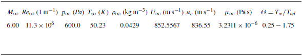


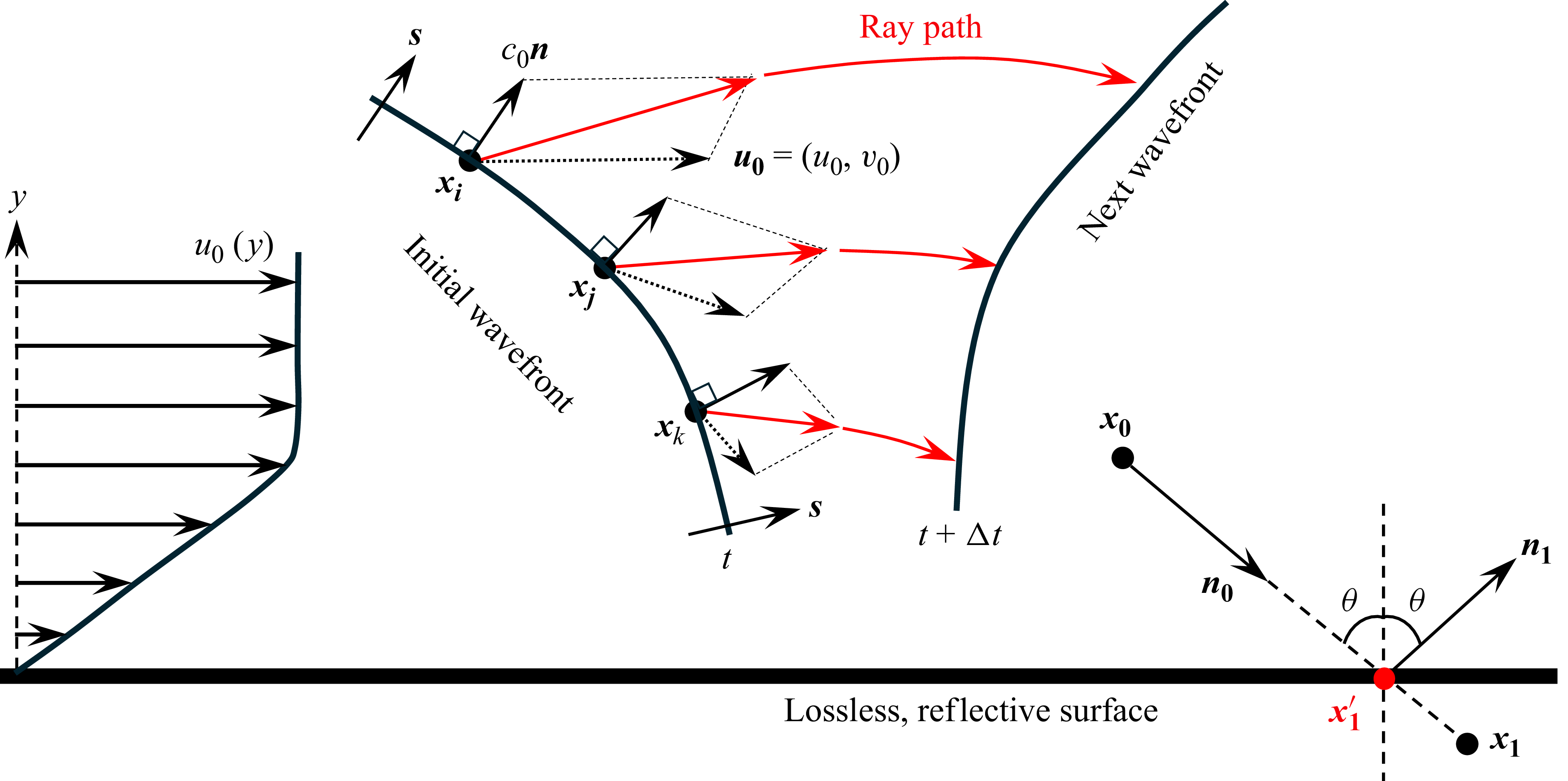


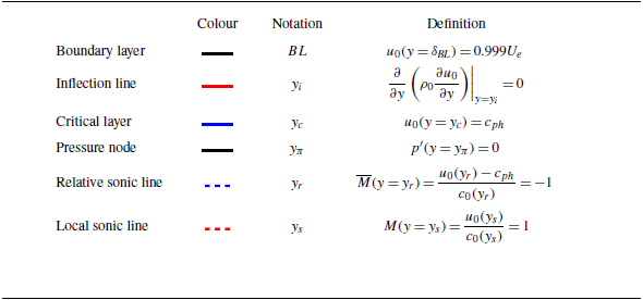


 Open access