


1. Introduction
Quasi-isodynamic (QI) stellarators (Gori, Lotz & Nührenberg Reference Gori, Lotz and Nührenberg1996) are a class of fusion devices that are being intensely investigated for their uniquely attractive properties, like intrinsic stability, robustness and good plasma confinement. What sets them apart from other optimised stellarators, on a purely technical level, is the topology of lines of constant magnetic field strength that close the short way around the torus (poloidally). In simple terms, the magnetic field of such devices roughly resembles a sequence of linked mirror devices, placed end-to-end and connected into a torus. The three-dimensional nature of this arrangement means that the shape of the magnetic geometry must be carefully optimised to ensure confinement of collisionless particle orbits.
These defining features bring a myriad of important consequences for the plasma physics of these devices, an immediate one being the complications arising in the theoretical description, computation and optimisation of their magnetohydrodynamic equilibria. To help with this, approximate solutions are essential to provide fundamental understanding and as starting points for further investigation. Solving the magnetic equilibrium problem near the innermost magnetic field line, i.e. the ‘magnetic axis’ of a stellarator, plays exactly this role. This will be the subject of our paper.
The ‘indirect’ or ‘inverse-coordinate’ approach to solving this problem can be formulated in magnetic coordinates to allow important symmetries of the magnetic field (quasi-symmetry or omnigenity) to be easily enforced (Garren & Boozer Reference Garren and Boozer1991b ). Compared with the ‘direct’ approach of Mercier (Mercier Reference Mercier1964; Solov’ev & Shafranov Reference Solov’ev and Shafranov1970) (where magnetic coordinates are an output of the calculation), the indirect approach is in some ways less intuitive, as many of the inputs are given in abstract quantities that do not have such a simple geometric interpretation. For the case of QI magnetic equilibria, the issue is more severe, as the quality of solutions is sensitive to basic geometric features, e.g. the axis shape and surface elongation, which have proved difficult to control. This can be overcome, to some extent, by careful choice of input parameters (Camacho Mata, Plunk & Jorge Reference Camacho Mata, Plunk and Jorge2022; Camacho Mata & Plunk Reference Camacho Mata and Plunk2023) or by an additional optimisation step, within the space of near-axis solutions (Jorge et al. Reference Jorge, Plunk, Drevlak, Landreman, Lobsien, Camacho and Helander2022).
An alternative approach, as pursued here, is to choose the inputs of the theory to be more geometrical, starting with the magnetic axis itself (zeroth order), solved using Frenet–Serret equations (Frenet Reference Frenet1852; Animov Reference Animov2001), and proceeding to the elliptical shaping parameters of the magnetic surfaces (first order). This approach can be viewed as an attempt to include some of the benefits of Mercier’s approach to make the inverse formulation more geometrically transparent.
The method was presented by Plunk (Reference Plunk2023), but so far, not described in detail elsewhere. Several papers have been written that use, in one form or another, configurations constructed using this methodology (Goodman et al. Reference Goodman, Xanthopoulos, Plunk, Smith, Nührenberg, Beidler, Henneberg, Roberg-Clark, Drevlak and Helander2024; Hindenlang, Plunk & Maj Reference Rodríguez and Plunk2024; Rodríguez et al. Reference Rodríguez and Plunk2024, Reference Rodríguez, Plunk and Jorge2025; Rodríguez & Plunk Reference Hindenlang, Plunk and Maj2024; Plunk et al. Reference Plunk, Drevlak, Rodríguez, Babin, Goodman and Hindenlang2025), giving further motivation to publish details about it.
In this work, we describe this geometric method to construct QI fields and demonstrate its flexibility to explore different classes of QI, characterised by magnetic axis topology and orders of axis curve flattening at field extrema. We begin with some essential background (§ 2), proceed to details of the method (§ 3.1) and then describe the overall ‘construction’ of the full solution to first order in the expansion, with examples. Finally, a survey of the conventional class of QI (‘half-helicity’) is performed, with emphasis on geometric properties and scaling behaviour with field period number $N$
. In the appendices, we describe the connection between our ‘hybrid’ indirect/direct approach and the original work of Mercier.
$N$
. In the appendices, we describe the connection between our ‘hybrid’ indirect/direct approach and the original work of Mercier.
2. Zeroth-order near-axis theory: magnetic axis shape and on-axis field strength
The near-axis expansion (NAE) (Plunk et al. Reference Plunk, Landreman and Helander2019; Camacho Mata et al. Reference Camacho Mata, Plunk and Jorge2022; Jorge et al. Reference Jorge, Plunk, Drevlak, Landreman, Lobsien, Camacho and Helander2022; Rodríguez & Plunk Reference Rodríguez and Plunk2023; Rodríguez et al. Reference Rodríguez, Plunk and Jorge2025) provides a theoretical framework for finding approximate stellarator equilibrium fields, valid in the neighbourhood of the magnetic axis. Global solutions with finite radius can then be ‘directly constructed’ (Landreman & Sengupta Reference Landreman and Sengupta2018; Plunk et al. Reference Plunk, Landreman and Helander2019) by evaluating the asymptotic description near the magnetic axis, at a specified distance (average minor radius). The resulting plasma boundary shape can be provided as input to a magnetohydrodynamic (MHD) equilibrium code like VMEC (Hirshman & Whitson Reference Hirshman and Whitson1983), GVEC (Hindenlang et al. Reference Hindenlang, Maj, Strumberger, Rampp and Sonnendrücker2019) or DESC (Dudt & Kolemen Reference Dudt and Kolemen2020) for further investigation. In this paper, we perform the expansion up to first order, starting in this section with the zeroth-order part, the magnetic axis and on-axis magnetic field strength.
We will focus on the simple case of a single magnetic trapping well per field period, i.e. with a single minimum in the field strength on axis, $B_0(\varphi )$
. We also assume stellarator symmetry (Dewar & Hudson Reference Dewar and Hudson1998), implying that the field extrema coincide with stellarator-symmetric points. By the convention used here, these are located at
$B_0(\varphi )$
. We also assume stellarator symmetry (Dewar & Hudson Reference Dewar and Hudson1998), implying that the field extrema coincide with stellarator-symmetric points. By the convention used here, these are located at $\varphi _{\mathrm{max}}^{(i)} = 2\pi i/N$
for maxima and
$\varphi _{\mathrm{max}}^{(i)} = 2\pi i/N$
for maxima and $(2 i + 1)\pi /N$
for minima, where
$(2 i + 1)\pi /N$
for minima, where $i$
is an integer and
$i$
is an integer and $\varphi$
is the Boozer toroidal angle (Boozer Reference Boozer1981; D’haeseleer Reference D’haeseleer1991).
$\varphi$
is the Boozer toroidal angle (Boozer Reference Boozer1981; D’haeseleer Reference D’haeseleer1991).
The magnetic axis is a closed space curve representing the central magnetic field line of the stellarator. The geometry of this curve affects the behaviour of the field. Most importantly, the curvature of the axis is directly linked to the gradients of the field strength. For this reason, the axis curves of a quasi-isodynamic stellarator have ‘flattening points’ (points of zero curvature) at extrema of the magnetic field strength along the axis; this flattening is necessary for poloidal closure of the contours of constant field strength $|\boldsymbol{B}|$
(Plunk et al. Reference Plunk, Landreman and Helander2019; Rodríguez et al. Reference Rodríguez, Plunk and Jorge2025).
$|\boldsymbol{B}|$
(Plunk et al. Reference Plunk, Landreman and Helander2019; Rodríguez et al. Reference Rodríguez, Plunk and Jorge2025).
This constraint on the curvature already makes the problem of constructing suitable curves a non-trivial part of constructing a QI configuration. In previous works on near-axis QI stellarators, magnetic axis curves that satisfy these flattening conditions were found by applying linear constraints to Fourier coefficients of the curve in cylindrical coordinates (see Camacho Mata et al. and Appendix A here). Curves constructed this way are closed and smooth by construction, and satisfy the required flattening conditions. The presence of these straight sections, however, make such curves sensitive to deformations. The torsion, in particular, is prone to singularities near flattening points (see Appendix A for a detailed discussion). Because torsion and other geometric properties of the axis curve directly control magnetic field properties such as the rotational transform and flux surface shaping, a level of control on these properties is desired that the conventional approach just described does not easily provide (see some further discussion in Appendix A).
In this work, to address the issues just discussed, we propose a method to construct the axis curve by prescribing curvature, $\kappa$
, and torsion,
$\kappa$
, and torsion, $\tau$
, as functions of the arc length
$\tau$
, as functions of the arc length $\ell$
(for simplicity,
$\ell$
(for simplicity, $\ell \in [0,2\pi )$
) along the curve, and solve the Frenet–Serret (FS) equations (Frenet Reference Frenet1852; Animov Reference Animov2001),
$\ell \in [0,2\pi )$
) along the curve, and solve the Frenet–Serret (FS) equations (Frenet Reference Frenet1852; Animov Reference Animov2001),
 \begin{equation} \frac {\text{d}\boldsymbol{x}_0}{\text{d}\ell }=\hat {\boldsymbol{t}},\quad \frac {\text{d}\hat {\boldsymbol{t}}}{\text{d}\ell }=\kappa \hat {\boldsymbol{\kappa }},\quad \frac {\text{d}\hat {\boldsymbol{\kappa }}}{\text{d}\ell }=-\kappa \hat {\boldsymbol{t}} + \tau \hat {\boldsymbol{\tau }},\quad \frac {\text{d}\hat {\boldsymbol{\tau }}}{\text{d}\ell }=-\tau \hat {\boldsymbol{\kappa }}, \end{equation}
where ${\boldsymbol{x}}_0$
is the axis curve,
${\boldsymbol{x}}_0$
is the axis curve, $\hat {\boldsymbol{t}}$
is its tangent and
$\hat {\boldsymbol{t}}$
is its tangent and $(\hat {\boldsymbol{\kappa }},\hat {\boldsymbol{\tau }})$
complete the orthonormal frame. For any functions
$(\hat {\boldsymbol{\kappa }},\hat {\boldsymbol{\tau }})$
complete the orthonormal frame. For any functions $\kappa$
and
$\kappa$
and $\tau$
, (2.1) may be integrated to obtain a curve, which is unique up to translations and rotations, i.e. initial conditions for the curve
$\tau$
, (2.1) may be integrated to obtain a curve, which is unique up to translations and rotations, i.e. initial conditions for the curve $\boldsymbol{x}_0$
and its frame (Banchoff & Lovett Reference Banchoff and Lovett2022, Theorem 3.4.1; do Carmo & Manfredo Reference Carmo and Manfredo2016, Ch. 1–5).
$\boldsymbol{x}_0$
and its frame (Banchoff & Lovett Reference Banchoff and Lovett2022, Theorem 3.4.1; do Carmo & Manfredo Reference Carmo and Manfredo2016, Ch. 1–5).
Treating curvature as an input to the curve construction ensures that the curve can have the desired flattening points. We can categorise different curves in terms of the order of the zeros of curvature, which we denote $(i,j)$
, referring to the field maxima and minima, respectively. Across some of these points, the curve undergoes inflection, by which we mean that the vector
$(i,j)$
, referring to the field maxima and minima, respectively. Across some of these points, the curve undergoes inflection, by which we mean that the vector $\text{d}\hat {\boldsymbol{t}}/\text{d}\ell$
flips direction discontinuously. In a QI field, inflection is mandatory at locations of minimum field strength (Plunk et al. Reference Plunk, Landreman and Helander2019; Rodríguez & Plunk Reference Rodríguez and Plunk2023). For this reason,
$\text{d}\hat {\boldsymbol{t}}/\text{d}\ell$
flips direction discontinuously. In a QI field, inflection is mandatory at locations of minimum field strength (Plunk et al. Reference Plunk, Landreman and Helander2019; Rodríguez & Plunk Reference Rodríguez and Plunk2023). For this reason, $\kappa$
is defined as ‘signed curvature’, which crosses zero at such points. By stellarator symmetry, the signed curvature is therefore odd about locations of field minima, while torsion is an even function. Furthermore,
$\kappa$
is defined as ‘signed curvature’, which crosses zero at such points. By stellarator symmetry, the signed curvature is therefore odd about locations of field minima, while torsion is an even function. Furthermore, $(\hat {\boldsymbol{t}}, \hat {\boldsymbol{\kappa }}, \hat {\boldsymbol{\tau }})$
must be defined as the signed Frenet frame (Plunk et al. Reference Plunk, Landreman and Helander2019; Rodríguez et al. Reference Rodríguez, Plunk and Jorge2025; Carroll, Köse & Sterling Reference Carroll, Köse and Sterling2013), i.e.
$(\hat {\boldsymbol{t}}, \hat {\boldsymbol{\kappa }}, \hat {\boldsymbol{\tau }})$
must be defined as the signed Frenet frame (Plunk et al. Reference Plunk, Landreman and Helander2019; Rodríguez et al. Reference Rodríguez, Plunk and Jorge2025; Carroll, Köse & Sterling Reference Carroll, Köse and Sterling2013), i.e. $(\hat {\boldsymbol{t}}\!, \hat {\boldsymbol{\kappa }}\!, \hat {\boldsymbol{\tau }}) = (\hat {\boldsymbol{t}}^{F}\!, s_\kappa \hat {\boldsymbol{\kappa }}^{F}\!, s_\kappa \hat {\boldsymbol{\tau }}^{F})$
, where
$(\hat {\boldsymbol{t}}\!, \hat {\boldsymbol{\kappa }}\!, \hat {\boldsymbol{\tau }}) = (\hat {\boldsymbol{t}}^{F}\!, s_\kappa \hat {\boldsymbol{\kappa }}^{F}\!, s_\kappa \hat {\boldsymbol{\tau }}^{F})$
, where $s_\kappa = \mathrm{sign}(\kappa )$
and
$s_\kappa = \mathrm{sign}(\kappa )$
and $(\hat {\boldsymbol{t}}^{F}, \hat {\boldsymbol{\kappa }}^{F}, \hat {\boldsymbol{\tau }}^{F})$
is the conventionally defined Frenet frame, i.e.
$(\hat {\boldsymbol{t}}^{F}, \hat {\boldsymbol{\kappa }}^{F}, \hat {\boldsymbol{\tau }}^{F})$
is the conventionally defined Frenet frame, i.e. $\hat {\boldsymbol{t}}^{F} = \boldsymbol{x}_0^\prime$
,
$\hat {\boldsymbol{t}}^{F} = \boldsymbol{x}_0^\prime$
, $\hat {\boldsymbol{\kappa }}^{F}=\boldsymbol{x}_0^{\prime \prime }/|\boldsymbol{x}_0^{\prime \prime }|$
and
$\hat {\boldsymbol{\kappa }}^{F}=\boldsymbol{x}_0^{\prime \prime }/|\boldsymbol{x}_0^{\prime \prime }|$
and $\hat {\boldsymbol{\tau }}^{F} = \hat {\boldsymbol{t}}^{F}\times \hat {\boldsymbol{\kappa }}^{F}$
, defined in the limiting sense approaching those points where
$\hat {\boldsymbol{\tau }}^{F} = \hat {\boldsymbol{t}}^{F}\times \hat {\boldsymbol{\kappa }}^{F}$
, defined in the limiting sense approaching those points where $|\boldsymbol{x}_0^{\prime \prime }| = 0$
and where primes denote derivatives with respect to
$|\boldsymbol{x}_0^{\prime \prime }| = 0$
and where primes denote derivatives with respect to $\ell$
.
$\ell$
.
The signed Frenet frame is by our convention continuous within a field period, i.e. $\ell \in [2\pi n/N,2\pi (n+1)/N)$
, where
$\ell \in [2\pi n/N,2\pi (n+1)/N)$
, where $n$
is an integer. In particular, field periods are taken to begin and end at locations of maximum field strength, and the FS equations are solved within a single field period with the full curve determined by continuation, using the
$n$
is an integer. In particular, field periods are taken to begin and end at locations of maximum field strength, and the FS equations are solved within a single field period with the full curve determined by continuation, using the $N$
-fold symmetry.
$N$
-fold symmetry.
An important property of the magnetic axis curve is its helicity, i.e. the number of times the signed normal rotates about the axis (Landreman & Sengupta Reference Landreman and Sengupta2019; Rodríguez et al. Reference Rodríguez, Sengupta and Bhattacharjee2022; Mata & Plunk Reference Camacho Mata and Plunk2023; Rodríguez et al. Reference Rodríguez, Plunk and Jorge2025) (also self-linking number (Fuller Reference Fuller1971; Moffatt & Ricca Reference Moffatt and Ricca1992; Fuller & Edgar Reference Fuller and Edgar1999)). We define the per-field-period helicity as $m = M/N$
, where
$m = M/N$
, where $M$
the total number of turns for all field periods. The per-period helicity can be any integer multiple of
$M$
the total number of turns for all field periods. The per-period helicity can be any integer multiple of $1/2$
(Camacho Mata & Plunk Reference Camacho Mata and Plunk2023; Rodríguez et al. Reference Rodríguez, Plunk and Jorge2025). There is no closed-form expression for helicity in terms of curvature and torsion, so the curve must first be constructed (by solving the FS equations) to compute the helicity.Footnote
1
$1/2$
(Camacho Mata & Plunk Reference Camacho Mata and Plunk2023; Rodríguez et al. Reference Rodríguez, Plunk and Jorge2025). There is no closed-form expression for helicity in terms of curvature and torsion, so the curve must first be constructed (by solving the FS equations) to compute the helicity.Footnote
1
Although the FS equations can, for arbitrary choice of $\tau$
and
$\tau$
and $\kappa$
, be integrated to obtain a space curve, this curve will generally not be closed. A further optimisation step is therefore required to achieve that (Garren & Boozer, Reference Garren and Boozer1991b
). The remainder of this section is dedicated to discussing the details of how to achieve axis closure. First, to ensure that axis curves can be constructed uniquely (excluding differences due to trivial translational and rotational freedoms), we will adopt a number of conventions.
$\kappa$
, be integrated to obtain a space curve, this curve will generally not be closed. A further optimisation step is therefore required to achieve that (Garren & Boozer, Reference Garren and Boozer1991b
). The remainder of this section is dedicated to discussing the details of how to achieve axis closure. First, to ensure that axis curves can be constructed uniquely (excluding differences due to trivial translational and rotational freedoms), we will adopt a number of conventions.
-
(i) Field periods are taken to begin and end at locations $\phi = 2 \pi n/N$
, where
$\phi$
is the cylindrical angle and
$n$
takes consecutive integer values. Lines of stellarator symmetry lie at these locations, as well as at their midpoints,
$\phi = \pi n/N$
.
$\phi = 2 \pi n/N$
, where
$\phi$
is the cylindrical angle and
$n$
takes consecutive integer values. Lines of stellarator symmetry lie at these locations, as well as at their midpoints,
$\phi = \pi n/N$
. -
(ii) The axis curve is centred at
$x=y=z=0$
; for
$N=1$
, the curve is positioned such that this point is half-way between the locations of the field maximum and minimum. -
(iii) The axis curve begins along the
$x$
-axis (the
$y$
and
$z$
components of
${\boldsymbol x}_0$
are zero at
$\ell = 0$
), i.e.
${\boldsymbol x}_0|_{\ell = 0} = (x_0, 0 , 0)$
. -
(iv) For the case
$N = 1$
, an additional rotational freedom (about a single axis of stellarator symmetry) is fixed by taking
${\boldsymbol{x}}_0\boldsymbol{\cdot }\hat {\boldsymbol{z}} = 0$
at
$\phi = \pi /2$
. This extra constraint is needed as the number of symmetry points in item (i), only two, are insufficient to uniquely define a plane.


2.1. Closure criteria for
$N = 1$

The method to numerically obtain closed space curves is to tune the curvature and torsion until a number of ‘closure criteria’ are satisfied to sufficient accuracy (Garren & Boozer Reference Garren and Boozer1991b
). Closure includes the three scalar criteria corresponding to ${\boldsymbol{x}}_0|_{\ell = 0} = {\boldsymbol{x}}_0|_{\ell = 2\pi }$
(the curve being closed), but also criteria associated with the periodicity of the frame (the frame being aligned),
${\boldsymbol{x}}_0|_{\ell = 0} = {\boldsymbol{x}}_0|_{\ell = 2\pi }$
(the curve being closed), but also criteria associated with the periodicity of the frame (the frame being aligned), $\hat {\boldsymbol{t}}|_{\ell = 0} = \hat {\boldsymbol{t}}|_{\ell = 2\pi }$
, etc. The ‘endpoint’ quantities are computed by integrating the FS equations, (2.1). The case of fractional helicity (i.e.
$\hat {\boldsymbol{t}}|_{\ell = 0} = \hat {\boldsymbol{t}}|_{\ell = 2\pi }$
, etc. The ‘endpoint’ quantities are computed by integrating the FS equations, (2.1). The case of fractional helicity (i.e. $m$
an integer plus
$m$
an integer plus $1/2$
) is a special one, as the periodicity conditions that the frame satisfies can involve a sign flip. For the
$1/2$
) is a special one, as the periodicity conditions that the frame satisfies can involve a sign flip. For the $N=1$
case, the signed normal
$N=1$
case, the signed normal $\hat {\boldsymbol{\kappa }}$
(and binormal,
$\hat {\boldsymbol{\kappa }}$
(and binormal, $\hat {\boldsymbol{\tau }}$
) will satisfy
$\hat {\boldsymbol{\tau }}$
) will satisfy $\hat {\boldsymbol{\kappa }}|_{\ell = 0} = -\hat {\boldsymbol{\kappa }}|_{\ell = 2\pi }$
if the helicity is fractional in this sense.
$\hat {\boldsymbol{\kappa }}|_{\ell = 0} = -\hat {\boldsymbol{\kappa }}|_{\ell = 2\pi }$
if the helicity is fractional in this sense.
There is a certain amount of redundant information in the closure constraint of the frame, which is, by construction, orthonormal. In particular, the minimal number of scalar criteria necessary to guarantee alignment of the frame is much lower than the nine scalar components of the frame vectors. In fact, it should only be three conditions, corresponding to the number of Euler angles necessary to fully describe the orientation of a rigid body. Thus, the closure for the most general class of $N=1$
curves would seem to require six free ‘shaping’ parameters in the functions
$N=1$
curves would seem to require six free ‘shaping’ parameters in the functions $\kappa$
and
$\kappa$
and $\tau$
(as many as closure conditions). However, to simplify things a bit, we only consider stellarator symmetric curves here.
$\tau$
(as many as closure conditions). However, to simplify things a bit, we only consider stellarator symmetric curves here.
To help reduce the number of necessary closure conditions, we note that stellarator symmetry constrains initial values for the frame and position of the curve, following convention (iii). Consider a geometric consequence of the helicity of the axis: at the minima of the magnetic field, assuming stellarator symmetry, the inflection implies $\hat {\boldsymbol{\tau }}$
is parallel to the radial unit vector (in cylindrical coordinates)
$\hat {\boldsymbol{\tau }}$
is parallel to the radial unit vector (in cylindrical coordinates) $\hat {\boldsymbol R}$
(
$\hat {\boldsymbol R}$
( $\phi = \pi /N$
, etc.) (Camacho Mata et al. Reference Camacho Mata, Plunk and Jorge2022; Rodríguez et al. Reference Rodríguez, Plunk and Jorge2025) – otherwise, the curvature would cause the axis to move radially outward on one side of the minimum and radially inward on the other side, violating stellarator symmetry. Hence, for integer helicity
$\phi = \pi /N$
, etc.) (Camacho Mata et al. Reference Camacho Mata, Plunk and Jorge2022; Rodríguez et al. Reference Rodríguez, Plunk and Jorge2025) – otherwise, the curvature would cause the axis to move radially outward on one side of the minimum and radially inward on the other side, violating stellarator symmetry. Hence, for integer helicity $m$
,
$m$
, $\hat {\boldsymbol{\tau }}$
must also be parallel to
$\hat {\boldsymbol{\tau }}$
must also be parallel to $\hat {\boldsymbol R}$
at
$\hat {\boldsymbol R}$
at $\ell =0$
(the frame will make an integer number of half-turns between field maxima and minima), while for fractional helicities,
$\ell =0$
(the frame will make an integer number of half-turns between field maxima and minima), while for fractional helicities, $\hat {\boldsymbol{\kappa }}$
is parallel to
$\hat {\boldsymbol{\kappa }}$
is parallel to $\hat {\boldsymbol R}$
at such locations (a relative quarter-turn will remain). So, the choice of alignment of the frame when initialising the Frenet construction has important influence on the helicity of the curve. In short,
$\hat {\boldsymbol R}$
at such locations (a relative quarter-turn will remain). So, the choice of alignment of the frame when initialising the Frenet construction has important influence on the helicity of the curve. In short, $\hat {\boldsymbol{\kappa }}$
or
$\hat {\boldsymbol{\kappa }}$
or $\hat {\boldsymbol{\tau }}$
can be aligned with
$\hat {\boldsymbol{\tau }}$
can be aligned with $\hat {\boldsymbol{x}}$
at
$\hat {\boldsymbol{x}}$
at $\ell =0$
depending on the desired helicity of the solution. In addition to the normal components of the Frenet–Serret frame, there is also rotational freedom in the tangent about
$\ell =0$
depending on the desired helicity of the solution. In addition to the normal components of the Frenet–Serret frame, there is also rotational freedom in the tangent about $\hat {\boldsymbol{x}}$
at
$\hat {\boldsymbol{x}}$
at $\ell =0$
. To uniquely choose this freedom, we shall rotate the final curve so as to satisfy condition (iv).
$\ell =0$
. To uniquely choose this freedom, we shall rotate the final curve so as to satisfy condition (iv).
With these initial conditions on the frame, we can then evaluate the closure criteria, which, using stellarator symmetry, can be applied at $\ell = \pi$
. From the symmetry of (A1), the
$\ell = \pi$
. From the symmetry of (A1), the $\hat {\boldsymbol{x}}$
component of
$\hat {\boldsymbol{x}}$
component of ${\boldsymbol{x}}_0$
is invariant under
${\boldsymbol{x}}_0$
is invariant under $\ell \rightarrow \pi -\ell$
, and closure of the curve only requires the other (odd) components to be zero (i.e. requires the point at
$\ell \rightarrow \pi -\ell$
, and closure of the curve only requires the other (odd) components to be zero (i.e. requires the point at $\ell =\pi$
to lie along the x-axis):
$\ell =\pi$
to lie along the x-axis):
 \begin{align} \hat {\boldsymbol{y}}\boldsymbol{\cdot }{\boldsymbol{x}}_0|_{\ell = \pi } = 0,\\[-10pt]\nonumber \end{align}
 \begin{align} \hat {\boldsymbol{z}}\boldsymbol{\cdot }{\boldsymbol{x}}_0|_{\ell = \pi } = 0. \end{align}
Similar arguments may be extended to the tangent and normal components of the frame (using (A2) instead of (A1) for the symmetry arguments). In both cases, the vectors must live in the plane normal to $\hat {\boldsymbol{R}}$
(or the x-axis by condition (iii)), so that the last two closure conditions are this way obtained:
$\hat {\boldsymbol{R}}$
(or the x-axis by condition (iii)), so that the last two closure conditions are this way obtained:
 \begin{align} \hat {\boldsymbol{x}}\boldsymbol{\cdot }\hat {\boldsymbol{t}}|_{\ell = \pi } = 0,\\[-10pt]\nonumber \end{align}
 \begin{align} \hat {\boldsymbol{x}}\boldsymbol{\cdot }\hat {\boldsymbol{\kappa }}|_{\ell = \pi } = 0. \end{align}
With four conditions to satisfy, we allow for four free “shaping” parameters for the magnetic axis curvature and torsion. An example of a suitable parametrisation is as follows:
 \begin{align} \kappa =& \left ( \kappa _1 \sin (N \ell ) + \kappa _2 \sin (2 N \ell ) \right )\cos ^2\left (\frac {N \ell }{2}\right ) \sin \left (\frac {N \ell }{2}\right)\!,\\[-10pt]\nonumber \end{align}
 \begin{align} \tau = & \tau _0 + \tau _1 \cos ( N \ell ) + \tau _2 \cos (2 N \ell ), \end{align}
This form of $\kappa$
corresponds to curves of the class
$\kappa$
corresponds to curves of the class $(2,3)$
: second-order zeros at the field maxima and third-order zeroes at the minima.
$(2,3)$
: second-order zeros at the field maxima and third-order zeroes at the minima.
In practice, of the five parameters ( $\kappa _1$
,
$\kappa _1$
, $\kappa _2$
,
$\kappa _2$
, $\tau _0$
,
$\tau _0$
, $\tau _1$
and
$\tau _1$
and $\tau _2$
), four can be used to satisfy closure criteria, leaving one left to define a one-parameter family of curves. We iteratively integrate FS equations, using a root solver, to obtain suitable coefficients. The desired helicity class (integer or half-integer) fixes the initial condition for the frame, but the actual helicity is only determined by inspection of the final solution. This method is sensitive to the initial guess (for shaping parameters) and not guaranteed to find all desired solutions even within a particular class, i.e. given field period number
$\tau _2$
), four can be used to satisfy closure criteria, leaving one left to define a one-parameter family of curves. We iteratively integrate FS equations, using a root solver, to obtain suitable coefficients. The desired helicity class (integer or half-integer) fixes the initial condition for the frame, but the actual helicity is only determined by inspection of the final solution. This method is sensitive to the initial guess (for shaping parameters) and not guaranteed to find all desired solutions even within a particular class, i.e. given field period number $N$
and helicity
$N$
and helicity $m$
. The curve obtained by this procedure will generally not comply with conventions (ii) and (iv), and thus, a final translation along the
$m$
. The curve obtained by this procedure will generally not comply with conventions (ii) and (iv), and thus, a final translation along the $x$
-axis and rotation about the
$x$
-axis and rotation about the $x$
-axis are applied.
$x$
-axis are applied.
A general comment about (2.3)–(2.4) and similar forms introduced here (2.6)–(2.8), (3.7) and (4.1): the inputs of the near axis construction that are functions of $\varphi$
are here parametrised using simple truncated Fourier series. These forms are straightforward to generalise, by including an arbitrary numbers of Fourier modes, and to handle arbitrary orders of zeros at field extrema, but this is left for future work. For present purposes, we focus on a low number of modes mostly for simplicity, but also following the principle that geometric simplicity is beneficial in stellarator design.
$\varphi$
are here parametrised using simple truncated Fourier series. These forms are straightforward to generalise, by including an arbitrary numbers of Fourier modes, and to handle arbitrary orders of zeros at field extrema, but this is left for future work. For present purposes, we focus on a low number of modes mostly for simplicity, but also following the principle that geometric simplicity is beneficial in stellarator design.
2.2. Closure criteria for
$N \geqslant 2$

The case $N \geqslant 2$
yields significant simplification as compared with the case
$N \geqslant 2$
yields significant simplification as compared with the case $N = 1$
. We integrate the FS equations over a single field period
$N = 1$
. We integrate the FS equations over a single field period $\ell \in [0, 2\pi /N]$
and derive a set of conditions to apply at the ends of this domain, with these conditions designed to ensure both that the curve itself closes (after
$\ell \in [0, 2\pi /N]$
and derive a set of conditions to apply at the ends of this domain, with these conditions designed to ensure both that the curve itself closes (after $N$
field periods) and that the frame is suitably periodic.
$N$
field periods) and that the frame is suitably periodic.
Let us describe how to use field periodicity to reduce the number of closure criteria. First, we start with a generally open curve, obtained by integrating (2.1), with its initial position along the x-axis following convention (iii). Rotational freedom about the $x$
-axis can be used to ensure the end of this curve lies in the
$x$
-axis can be used to ensure the end of this curve lies in the $x$
–
$x$
– $y$
plane (which is required by periodicity), i.e. defining
$y$
plane (which is required by periodicity), i.e. defining ${\boldsymbol{x}}_0|_{\ell = 2\pi /N} = (x_1, y_1, z_1)$
, we have
${\boldsymbol{x}}_0|_{\ell = 2\pi /N} = (x_1, y_1, z_1)$
, we have $z_1 = 0$
. Then, rotational freedom about an axis parallel to the z-axis, running through the initial point
$z_1 = 0$
. Then, rotational freedom about an axis parallel to the z-axis, running through the initial point $(x_0, 0, 0)$
, and translational freedom (
$(x_0, 0, 0)$
, and translational freedom ( $x_0$
) can be used to ensure that the end of the curve is located at
$x_0$
) can be used to ensure that the end of the curve is located at $\phi = 2\pi /N$
, i.e.
$\phi = 2\pi /N$
, i.e. $y_1/x_1 = \tan (2\pi /N)$
. Therefore, the closure of the curve
$y_1/x_1 = \tan (2\pi /N)$
. Therefore, the closure of the curve ${\boldsymbol{x}}_0|_{\ell = 2\pi } = {\boldsymbol{x}}_0|_{\ell = 0}$
is achieved simply by
${\boldsymbol{x}}_0|_{\ell = 2\pi } = {\boldsymbol{x}}_0|_{\ell = 0}$
is achieved simply by $N$
-fold periodic extension, i.e. by connecting
$N$
-fold periodic extension, i.e. by connecting $N$
copies of the single-period curve end-to-end. With closure satisfied, only the continuity of the frame is left to be enforced.
$N$
copies of the single-period curve end-to-end. With closure satisfied, only the continuity of the frame is left to be enforced.
At this stage (see figure 1), there remains a single rotational freedom of the axis segment that preserves the location of the initial and final points ( ${\boldsymbol{x}}_0|_{\ell = 0}$
and
${\boldsymbol{x}}_0|_{\ell = 0}$
and ${\boldsymbol{x}}_0|_{\ell = 2\pi /N}$
), namely rotation about the line connecting these two points, by an angle
${\boldsymbol{x}}_0|_{\ell = 2\pi /N}$
), namely rotation about the line connecting these two points, by an angle $\zeta$
. Because this rotation is not aligned with the
$\zeta$
. Because this rotation is not aligned with the $x$
-axis, this rotation will actually change the initial orientation of the frame and, thus, we can use this degree of freedom towards alignment of the frame. To completely align the frames at the end and beginning of the period (up to a sign to allow for half-helicity curves), we impose three scalar constraints (i.e. three Euler angles of the frame):
$x$
-axis, this rotation will actually change the initial orientation of the frame and, thus, we can use this degree of freedom towards alignment of the frame. To completely align the frames at the end and beginning of the period (up to a sign to allow for half-helicity curves), we impose three scalar constraints (i.e. three Euler angles of the frame):
 \begin{align} {\hat {\boldsymbol{\kappa }}|_{\ell =2\pi /N}\boldsymbol{\cdot }{{\boldsymbol{\textsf{R}}}}_{z}(2\pi /N)\boldsymbol{\cdot }\hat {\boldsymbol{t}}|_{\ell =0}} = 0,\\[-10pt]\nonumber \end{align}
 \begin{align} {\hat {\boldsymbol{\tau }}|_{\ell =2\pi /N}\boldsymbol{\cdot }{{\boldsymbol{\textsf{R}}}}_{z}(2\pi /N)\boldsymbol{\cdot }\hat {\boldsymbol{t}}|_{\ell =0}} = 0,\\[-10pt]\nonumber \end{align}
 \begin{align} {\hat {\boldsymbol{\tau }}|_{\ell =2\pi /N}\boldsymbol{\cdot }{{\boldsymbol{\textsf{R}}}}_{z}(2\pi /N)\boldsymbol{\cdot }\hat {\boldsymbol{\kappa }}|_{\ell =0}} = 0, \end{align}
where ${{\boldsymbol{\textsf{R}}}}_{z}(2\pi /N)$
is the operator that performs rotation by the angle
${{\boldsymbol{\textsf{R}}}}_{z}(2\pi /N)$
is the operator that performs rotation by the angle $2\pi /N$
about the
$2\pi /N$
about the $z$
-axis so that the frame at the endpoint can be compared with the initial one.
$z$
-axis so that the frame at the endpoint can be compared with the initial one.
Diagram illustrating elements of curve closure. Example of an $N=3$
half-helicity curve with the main geometric elements considered for the closure of the axis, including the convention. In black, one field period of the axis from
$N=3$
half-helicity curve with the main geometric elements considered for the closure of the axis, including the convention. In black, one field period of the axis from $\ell =0$
to
$\ell =0$
to $\ell =2\pi /3$
, continued in grey. The
$\ell =2\pi /3$
, continued in grey. The $x,\,y,\,z$
frame is given as a reference.
$x,\,y,\,z$
frame is given as a reference.

To satisfy the three constraints, $\zeta$
provides one degree of freedom so two further free shaping parameters (by simple counting argument) are required as part of the curvature and torsion functions
$\zeta$
provides one degree of freedom so two further free shaping parameters (by simple counting argument) are required as part of the curvature and torsion functions $\kappa$
and
$\kappa$
and $\tau$
(consistent with Appendix B of Garren & Boozer (Reference Garren and Boozer1991a
)); as an example, we consider the following forms:
$\tau$
(consistent with Appendix B of Garren & Boozer (Reference Garren and Boozer1991a
)); as an example, we consider the following forms:
 \begin{align} \kappa = &\ \ \kappa _1 \cos ^2\left (\frac {N \ell }{2}\right ) \sin \left (\frac {N \ell }{2}\right )\sin (N \ell ),\\[-10pt]\nonumber \end{align}
 \begin{align} \tau =\ & \tau _0 + \tau _1 \cos ( N \ell ), \end{align}
where $\kappa _1$
,
$\kappa _1$
, $\tau _0$
and
$\tau _0$
and $\tau _1$
are constants. This form of
$\tau _1$
are constants. This form of $\kappa$
(used for the figure-8 configuration of Plunk et al. Reference Plunk, Drevlak, Rodríguez, Babin, Goodman and Hindenlang2025) is also of the
$\kappa$
(used for the figure-8 configuration of Plunk et al. Reference Plunk, Drevlak, Rodríguez, Babin, Goodman and Hindenlang2025) is also of the $(2,3)$
class. Two of the three free constants are determined by satisfaction of the closure conditions, leaving a single parameter to parametrise a family of curves. Just like the
$(2,3)$
class. Two of the three free constants are determined by satisfaction of the closure conditions, leaving a single parameter to parametrise a family of curves. Just like the $N=1$
case, the method used for
$N=1$
case, the method used for $N \geqslant 2$
, and, in particular, the search for appropriate parameters, is sensitive to the initial guess, but we have not yet found evidence of multiple branches of solutions within a single class (given field period number
$N \geqslant 2$
, and, in particular, the search for appropriate parameters, is sensitive to the initial guess, but we have not yet found evidence of multiple branches of solutions within a single class (given field period number $N$
and helicity
$N$
and helicity $m$
).
$m$
).
As a final consideration, we note that, although we are interested in the case of stellarator symmetry, the previous methodology for curve construction is actually capable of treating the general problem where symmetry is broken, by simply using more general (non-symmetric) curvature and torsion functions. This is because stellarator symmetry actually requires the initial frame to have a particular alignment with respect to $\hat {\boldsymbol{x}}$
, so that the value of
$\hat {\boldsymbol{x}}$
, so that the value of $\zeta$
obtained by the solution method is automatically constrained to satisfy this given symmetric curvature and torsion functions. For non-symmetric curvature and torsion,
$\zeta$
obtained by the solution method is automatically constrained to satisfy this given symmetric curvature and torsion functions. For non-symmetric curvature and torsion, $\zeta$
instead provides a continuous freedom for parametrising the bigger space of non-symmetric curves.
$\zeta$
instead provides a continuous freedom for parametrising the bigger space of non-symmetric curves.
2.3. Complete zeroth-order solution
Once the axis curve has been specified, the solution to zeroth order in the NAE is completed by also specifying the magnetic field strength dependence along the magnetic axis. Stellarator symmetry requires an even function, for instance,
 \begin{equation} B_0 = 1 + \varDelta \cos (N \ell ) + \varDelta \cos (2N \ell )/4, \end{equation}
defined such that $B_0^{\prime \prime } = 0$
at field strength minima, e.g.
$B_0^{\prime \prime } = 0$
at field strength minima, e.g. $\ell =\pi /N$
, for reasons of stability and maximum-
$\ell =\pi /N$
, for reasons of stability and maximum- $\mathcal{J}$
(Rodríguez et al. Reference Rodríguez, Helander and Goodman2024; Plunk et al. Reference Plunk, Drevlak, Rodríguez, Babin, Goodman and Hindenlang2025). The parameter
$\mathcal{J}$
(Rodríguez et al. Reference Rodríguez, Helander and Goodman2024; Plunk et al. Reference Plunk, Drevlak, Rodríguez, Babin, Goodman and Hindenlang2025). The parameter $\varDelta = (B_0(0)-B_0(\pi /N))/2$
controls the mirror ratio; note the mean
$\varDelta = (B_0(0)-B_0(\pi /N))/2$
controls the mirror ratio; note the mean $\langle B_0 \rangle _\ell = 1$
. Finally, the relationship between axis length and Boozer toroidal angle
$\langle B_0 \rangle _\ell = 1$
. Finally, the relationship between axis length and Boozer toroidal angle $\varphi$
is determined (Landreman & Sengupta Reference Landreman and Sengupta2018; Plunk et al. Reference Plunk, Landreman and Helander2019):
$\varphi$
is determined (Landreman & Sengupta Reference Landreman and Sengupta2018; Plunk et al. Reference Plunk, Landreman and Helander2019):
 \begin{equation} \frac {\text{d}\varphi }{\text{d}\ell }= \frac {B_0}{|G_0|}, \hspace {0.3in} |G_0| = \frac {N}{2\pi }\int _0^{2\pi /N} B_0\,\text{d}\ell , \end{equation}
where $G_0$
is the zeroth-order Boozer poloidal current function.
$G_0$
is the zeroth-order Boozer poloidal current function.
3. First order: magnetic surface shaping
To complete the construction of the configuration, we must solve the so-called ‘ $\sigma$
-equation’ (Garren & Boozer Reference Garren and Boozer1991b; Landreman, Sengupta & Plunk Reference Landreman, Sengupta and Plunk2019), depending on several given inputs,
$\sigma$
-equation’ (Garren & Boozer Reference Garren and Boozer1991b; Landreman, Sengupta & Plunk Reference Landreman, Sengupta and Plunk2019), depending on several given inputs,
 \begin{equation} \sigma ^{\prime } + ({{\kern0.1em\iota\kern-0.38em^{_{\rule{4.5pt}{.4pt}}}}}_0 -\alpha ^{\prime })\left (\sigma ^{2}+ 1 + \bar {e}^2 \right ) + 2 G_{0} \tau \bar {e}/B_0 = 0, \end{equation}
where $\alpha$
and
$\alpha$
and $\bar {e}$
are functions of
$\bar {e}$
are functions of $\varphi$
(Plunk et al. Reference Plunk, Landreman and Helander2019; Camacho Mata et al. Reference Camacho Mata, Plunk and Jorge2022; Rodríguez et al. Reference Rodríguez, Plunk and Jorge2025), and
$\varphi$
(Plunk et al. Reference Plunk, Landreman and Helander2019; Camacho Mata et al. Reference Camacho Mata, Plunk and Jorge2022; Rodríguez et al. Reference Rodríguez, Plunk and Jorge2025), and ${{\kern0.1em\iota\kern-0.38em^{_{\rule{4.5pt}{.4pt}}}}}_0$
is the rotational transform on axis; note we have assumed zero toroidal current for simplicity. The solution to this equation determines the surface shape via the components of the first-order coordinate mapping,
${{\kern0.1em\iota\kern-0.38em^{_{\rule{4.5pt}{.4pt}}}}}_0$
is the rotational transform on axis; note we have assumed zero toroidal current for simplicity. The solution to this equation determines the surface shape via the components of the first-order coordinate mapping,
 \begin{align} X_{1} &= \sqrt {\frac {2\bar {e}}{B_0}} \cos {[\theta - \alpha (\varphi ) ]},\\[-10pt]\nonumber \end{align}
 \begin{align} Y_{1} &= \sqrt {\frac {2}{B_0\bar {e}}} \left ( \sin {[\theta - \alpha (\varphi )]} + \sigma (\varphi ) \cos {[\theta - \alpha (\varphi)]}\right)\!, \end{align}
which enters the coordinate mapping as follows:
 \begin{equation} \boldsymbol{x} \approx \boldsymbol{x}_{0} + \epsilon \left ( X_{1}\boldsymbol{n} + Y_{1}\boldsymbol{b} \right)\!, \end{equation}
where $\epsilon =\sqrt {\psi }$
.Footnote
2
The function
$\epsilon =\sqrt {\psi }$
.Footnote
2
The function $\sigma$
controls rotation of the cross-sections, as well as the elongation of the surrounding elliptical cross-sections (Rodríguez Reference Rodríguez2023). Elongation (of the elliptical cross sections) is a particularly sensitive feature of QI configurations that are derived from NAE theory. The difficulty arises in maintaining the poloidal closure of the contours of
$\sigma$
controls rotation of the cross-sections, as well as the elongation of the surrounding elliptical cross-sections (Rodríguez Reference Rodríguez2023). Elongation (of the elliptical cross sections) is a particularly sensitive feature of QI configurations that are derived from NAE theory. The difficulty arises in maintaining the poloidal closure of the contours of $|\boldsymbol{B}|$
, which can most easily be achieved by simply squeezing the ellipses along the normal direction to the axis (reducing poloidal variation of the field). Formally, the lack of control of elongation comes from
$|\boldsymbol{B}|$
, which can most easily be achieved by simply squeezing the ellipses along the normal direction to the axis (reducing poloidal variation of the field). Formally, the lack of control of elongation comes from $\sigma$
being an unknown of (3.1) (alongside the rotational transform), and thus elongation, which depends on
$\sigma$
being an unknown of (3.1) (alongside the rotational transform), and thus elongation, which depends on $\sigma$
, has so far been obtained as an output of the construction. Although the control of torsion has been shown to be a plausible way of limiting this shaping (Camacho Mata et al. Reference Camacho Mata, Plunk and Jorge2022; Camacho Mata & Plunk Reference Camacho Mata and Plunk2023) by limiting the size of
$\sigma$
, has so far been obtained as an output of the construction. Although the control of torsion has been shown to be a plausible way of limiting this shaping (Camacho Mata et al. Reference Camacho Mata, Plunk and Jorge2022; Camacho Mata & Plunk Reference Camacho Mata and Plunk2023) by limiting the size of $\sigma$
, we here consider an alternative approach.
$\sigma$
, we here consider an alternative approach.
We propose a way to solve the $\sigma$
equation using elongation as input, instead of the function
$\sigma$
equation using elongation as input, instead of the function $\bar {e}$
, which is used conventionally (Landreman et al. Reference Landreman, Sengupta and Plunk2019; Plunk et al. Reference Plunk, Landreman and Helander2019). The approach can be regarded as a hybrid with Mercier’s direct approach, in which the shape of flux surfaces is directly controlled in the near-axis description (see some further discussion of this in Appendix B). The elongation
$\bar {e}$
, which is used conventionally (Landreman et al. Reference Landreman, Sengupta and Plunk2019; Plunk et al. Reference Plunk, Landreman and Helander2019). The approach can be regarded as a hybrid with Mercier’s direct approach, in which the shape of flux surfaces is directly controlled in the near-axis description (see some further discussion of this in Appendix B). The elongation $E(\varphi )$
of the elliptical cross-section is
$E(\varphi )$
of the elliptical cross-section is
 \begin{align} E(\varphi ) &= \frac {1}{2}\left (\rho + \sqrt {\rho ^2-4}\right)\!,\\[-10pt]\nonumber \end{align}
 \begin{align} \quad \rho &= \bar {e} + \frac {1}{\bar {e}}(1 + \sigma ^2). \end{align}
The ‘elongation profile’ (see a geometric interpretation in Appendix B) is thus set by the function $\rho$
, which, for the class of configurations considered here, is chosen to have the following form:
$\rho$
, which, for the class of configurations considered here, is chosen to have the following form:
 \begin{equation} \rho = \sum _n \rho _n \cos (n N \varphi ), \end{equation}
where $\rho _n$
are constants chosen such that
$\rho _n$
are constants chosen such that $\rho \geqslant 2$
is satisfied for all
$\rho \geqslant 2$
is satisfied for all $\varphi$
.
$\varphi$
.
There is one more function that is part of the input at first order, namely the function $\alpha (\varphi )$
, see (3.2)–(3.3) and its appearance in (3.1). This phase angle controls the deviation of the field from the ideal QI limit (Plunk et al. Reference Plunk, Landreman and Helander2019). However, to minimise the deviation from QI, there is little freedom in this function when stellarator symmetry is assumed and it has so far seemed adequate to assume a sufficiently smooth form that avoids twist in the configurations (Camacho Mata et al. Reference Camacho Mata, Plunk and Jorge2022). A sufficiently high degree of smoothness also ensures good behaviour at higher order NAE, as described by Rodríguez et al. (Reference Rodríguez, Plunk and Jorge2025).
$\alpha (\varphi )$
, see (3.2)–(3.3) and its appearance in (3.1). This phase angle controls the deviation of the field from the ideal QI limit (Plunk et al. Reference Plunk, Landreman and Helander2019). However, to minimise the deviation from QI, there is little freedom in this function when stellarator symmetry is assumed and it has so far seemed adequate to assume a sufficiently smooth form that avoids twist in the configurations (Camacho Mata et al. Reference Camacho Mata, Plunk and Jorge2022). A sufficiently high degree of smoothness also ensures good behaviour at higher order NAE, as described by Rodríguez et al. (Reference Rodríguez, Plunk and Jorge2025).
Because our method of solving the $\sigma$
equation requires both variation in
$\sigma$
equation requires both variation in $\bar {e}$
and the ability to enforce QI symmetry by choice of
$\bar {e}$
and the ability to enforce QI symmetry by choice of $\rho$
, it does not seem applicable to the case of quasi-symmetry; indeed, it is apparently limited only to the case of stellarator symmetric QI stellarators.
$\rho$
, it does not seem applicable to the case of quasi-symmetry; indeed, it is apparently limited only to the case of stellarator symmetric QI stellarators.
3.1. Solution method
As is generally the case with the inverse approach to near-axis theory, the first-order problem may be solved by finding values of $\iota _0$
for which the solution of (3.1) yields periodic solutions of
$\iota _0$
for which the solution of (3.1) yields periodic solutions of $\sigma$
, i.e.
$\sigma$
, i.e. $\sigma (0) = \sigma (2\pi /N) = 0$
, assuming stellarator symmetry. The key difference here is the use of
$\sigma (0) = \sigma (2\pi /N) = 0$
, assuming stellarator symmetry. The key difference here is the use of $\rho$
instead of
$\rho$
instead of $\bar {e}$
as an input. We do not attempt here to show that this alternative problem specification is well posed, as it actually is not, with some inputs yielding no solutions. However, the solution method is well behaved in the sense that solutions can be rapidly found in a similar way as conventionally done (using
$\bar {e}$
as an input. We do not attempt here to show that this alternative problem specification is well posed, as it actually is not, with some inputs yielding no solutions. However, the solution method is well behaved in the sense that solutions can be rapidly found in a similar way as conventionally done (using $\bar {e}$
as an input) and the boundary in the input parameter space where solutions become invalid is identifiable, as described later.
$\bar {e}$
as an input) and the boundary in the input parameter space where solutions become invalid is identifiable, as described later.
To obtain the desired form of (3.1) (see (B3)), we simply need to express $\bar {e}$
in terms of
$\bar {e}$
in terms of $\sigma$
and
$\sigma$
and $\rho$
,
$\rho$
,
 \begin{align} \bar {e} = \frac {1}{2}\left (\rho - \sqrt {\rho ^2 - 4(1+\sigma ^2)} \right ), \end{align}
and substitute it into (3.1) to eliminate $\bar {e}$
. Here, we find two limitations of the approach. First, we have chosen the smaller root for
$\bar {e}$
. Here, we find two limitations of the approach. First, we have chosen the smaller root for $\bar {e}$
, corresponding to elongation of the ellipses in the conventional sense, i.e. in the binormal direction. This is a limitation of the method, excluding cases where elongation passes from the conventional to unconventional (elongated in the direction of the normal vector) sense. This does not appear to be a practical limitation, as the overwhelming majority of cases studied so far have conventional elongation that only ever approaches
$\bar {e}$
, corresponding to elongation of the ellipses in the conventional sense, i.e. in the binormal direction. This is a limitation of the method, excluding cases where elongation passes from the conventional to unconventional (elongated in the direction of the normal vector) sense. This does not appear to be a practical limitation, as the overwhelming majority of cases studied so far have conventional elongation that only ever approaches $1$
at specific locations in
$1$
at specific locations in $\varphi$
.
$\varphi$
.
A more significant downside of the method is that, even with $\rho \geqslant 2$
, a real solution to the equation may not exist. This occurs whenever
$\rho \geqslant 2$
, a real solution to the equation may not exist. This occurs whenever $\sigma$
is sufficiently large, which by inspecting (3.1) will tend to happen when the final source term is large, i.e. when the axis torsion is large, or when
$\sigma$
is sufficiently large, which by inspecting (3.1) will tend to happen when the final source term is large, i.e. when the axis torsion is large, or when $\bar {e}$
is large. However, reducing
$\bar {e}$
is large. However, reducing $\rho$
, though it reduces
$\rho$
, though it reduces $\bar {e}$
, exacerbates the problem in (3.8). In practice, this issue limits how small
$\bar {e}$
, exacerbates the problem in (3.8). In practice, this issue limits how small $\rho$
(and therefore plasma elongation) can be taken to obtain valid solutions for
$\rho$
(and therefore plasma elongation) can be taken to obtain valid solutions for $\sigma$
. To cope with this, the requirement
$\sigma$
. To cope with this, the requirement
 \begin{equation} \rho ^2 \geqslant 4 (1+\sigma ^2), \end{equation}
which depends on $\sigma$
, must be enforced by checking numerical solutions. Overall, we have lost the uniqueness and existence properties of the standard approach to the solution of the
$\sigma$
, must be enforced by checking numerical solutions. Overall, we have lost the uniqueness and existence properties of the standard approach to the solution of the $\sigma$
-equation (Landreman et al. Reference Landreman, Sengupta and Plunk2019), but have gained control of the geometric shaping.
$\sigma$
-equation (Landreman et al. Reference Landreman, Sengupta and Plunk2019), but have gained control of the geometric shaping.
We remark that the use of elongation explicitly in the solution process is reminiscent of the original near-axis expansion of Mercier (Reference Mercier1964). We have investigated this connection in some depth, but leave these details for Appendix B.
4. Constructing QI configurations
We now turn to practical considerations for the actual construction of full solutions to first order. The inputs at first order are considered as:
-
(i) the shape of the magnetic axis
${\boldsymbol{x}}_0$
(provided in terms of
$\kappa$
and
$\tau$
); -
(ii) the form of the on-axis magnetic field strength
$B_0(\varphi )$
; and -
(iii) the elongation profile
$\rho (\varphi )$
.


During construction of the magnetic axis, we also fix key quantities like the field periodicity $N$
, the orders of zeros of the signed curvature at field maxima and minima, and axis helicity
$N$
, the orders of zeros of the signed curvature at field maxima and minima, and axis helicity $m$
Footnote
3
. For this paper, we focus on the forms of
$m$
Footnote
3
. For this paper, we focus on the forms of $\kappa$
,
$\kappa$
, $\tau$
and
$\tau$
and $B_0$
given in § 2, meaning that the orders of curvature zeros are
$B_0$
given in § 2, meaning that the orders of curvature zeros are $2$
and
$2$
and $3$
at the maxima and minima, respectively. Many other forms are possible (and many have been implemented), but we will not attempt to list them here. We note that an even order at field maxima (e.g.
$3$
at the maxima and minima, respectively. Many other forms are possible (and many have been implemented), but we will not attempt to list them here. We note that an even order at field maxima (e.g. $2$
) is consistent with analyticity only for the case of fractional helicity (
$2$
) is consistent with analyticity only for the case of fractional helicity ( $m = 1/2, 3/2, \ldots$
) (Camacho Mata et al. Reference Camacho Mata, Plunk and Jorge2022; Rodríguez et al. Reference Rodríguez, Plunk and Jorge2025). For present purposes, analyticity is not a major concern and it is noteworthy that the method is capable of treating more general (non-analytic) classes of curves. It is even possible to have even orders of zero at inflection points as a sign change in the curvature is sufficient for inflection of the curves obtained from solving the FS equations.
$m = 1/2, 3/2, \ldots$
) (Camacho Mata et al. Reference Camacho Mata, Plunk and Jorge2022; Rodríguez et al. Reference Rodríguez, Plunk and Jorge2025). For present purposes, analyticity is not a major concern and it is noteworthy that the method is capable of treating more general (non-analytic) classes of curves. It is even possible to have even orders of zero at inflection points as a sign change in the curvature is sufficient for inflection of the curves obtained from solving the FS equations.
To illustrate the flexibility of our method, we show a number of configurations in table 1 representing a range of values of $N$
and
$N$
and $m$
. To demonstrate how elongation can be controlled with our method, we choose all of these to have uniform elongation, i.e.
$m$
. To demonstrate how elongation can be controlled with our method, we choose all of these to have uniform elongation, i.e. $\rho = \rho _0 \sim 4$
–
$\rho = \rho _0 \sim 4$
– $5$
among these examples. For low values of
$5$
among these examples. For low values of $\rho _0$
, the limit is approached where the criterion of (3.9) is marginally satisfied. Interestingly, the function
$\rho _0$
, the limit is approached where the criterion of (3.9) is marginally satisfied. Interestingly, the function $\bar {e}$
develops cusp-like behaviour at the value of
$\bar {e}$
develops cusp-like behaviour at the value of $\varphi$
where
$\varphi$
where $\sigma ^2$
approaches
$\sigma ^2$
approaches $\rho _0^2/4-1$
. The elongation remains smooth (by construction), underscoring the fact that such configurations remain geometrically simple in a sense, despite being potentially difficult to realise with a conventional approach that supplies Fourier coefficients of
$\rho _0^2/4-1$
. The elongation remains smooth (by construction), underscoring the fact that such configurations remain geometrically simple in a sense, despite being potentially difficult to realise with a conventional approach that supplies Fourier coefficients of $\bar {e}$
as input.
$\bar {e}$
as input.
A view of configurations with varying field period number $N$
and axis helicity
$N$
and axis helicity $m$
. Noteworthy cases that have been studied previously include
$m$
. Noteworthy cases that have been studied previously include $(N, m) = (1, 1)$
(Plunk et al. Reference Plunk, Landreman and Helander2019),
$(N, m) = (1, 1)$
(Plunk et al. Reference Plunk, Landreman and Helander2019), $(N, m) = (2, 1/2)$
(Plunk et al. Reference Plunk, Drevlak, Rodríguez, Babin, Goodman and Hindenlang2025) and the ever popular choice
$(N, m) = (2, 1/2)$
(Plunk et al. Reference Plunk, Drevlak, Rodríguez, Babin, Goodman and Hindenlang2025) and the ever popular choice $(N, m) = (4, 1/2)$
used in present day integrated QI optimisation, e.g. Goodman et al. (Reference Goodman, Xanthopoulos, Plunk, Smith, Nührenberg, Beidler, Henneberg, Roberg-Clark, Drevlak and Helander2024).
$(N, m) = (4, 1/2)$
used in present day integrated QI optimisation, e.g. Goodman et al. (Reference Goodman, Xanthopoulos, Plunk, Smith, Nührenberg, Beidler, Henneberg, Roberg-Clark, Drevlak and Helander2024).

4.1. Exotic QI
To further demonstrate the flexibility of the solution method, we show examples of a few QI configuration of the ‘knotatron’ type (Hudson, Startsev & Feibush Reference Hudson, Startsev and Feibush2014), where the plasma volume is knotted. Knotted axis shapes can be found with the method already described. This may appear disallowed by assumption (i), which would seem to imply conventional axis shapes, where a single period of the plasma equilibrium occupies a sector spanning an interval of $2\pi /N$
in
$2\pi /N$
in $\phi$
. In actuality, assumption (i) only requires the beginning and end of a field period to span this interval, and makes no restrictions on what happens in between. This allows axis shapes, for instance, where the curve spans a total angular distance of
$\phi$
. In actuality, assumption (i) only requires the beginning and end of a field period to span this interval, and makes no restrictions on what happens in between. This allows axis shapes, for instance, where the curve spans a total angular distance of $-2\pi (N-1)/N$
, such that it travels in the negative direction in
$-2\pi (N-1)/N$
, such that it travels in the negative direction in $\phi$
(
$\phi$
( $\text{d}\phi /\text{d}\ell \lt 0$
), and can therefore overlap and link with other field periods of the curve. The frame at the start and end of a field period can satisfy the closure criteria by being anti-aligned in this case.
$\text{d}\phi /\text{d}\ell \lt 0$
), and can therefore overlap and link with other field periods of the curve. The frame at the start and end of a field period can satisfy the closure criteria by being anti-aligned in this case.
A concrete example of all this is the $N=3$
trefoil knot, obtained when the axis curve begins at
$N=3$
trefoil knot, obtained when the axis curve begins at $\phi = 0$
, proceeds clockwise and ends at
$\phi = 0$
, proceeds clockwise and ends at $\phi = 2\pi /3$
. Two more configurations following a similar pattern are found with
$\phi = 2\pi /3$
. Two more configurations following a similar pattern are found with $N = 4$
and
$N = 4$
and $N = 5$
, as also shown in figure 2. These have increasingly large aspect ratio, taking their effective major radius to be set by the length of the magnetic axis curve, i.e.
$N = 5$
, as also shown in figure 2. These have increasingly large aspect ratio, taking their effective major radius to be set by the length of the magnetic axis curve, i.e. $R_{\mathrm{eff}} = L/(2\pi ) = 1$
. Not much is known about such knotted QI configurations, but non-QI knotted stellarators have been shown in the past (Garren & Boozer Reference Garren and Boozer1991b
; Hudson et al. Reference Hudson, Startsev and Feibush2014) and it is possible now to investigate such configurations beyond near-axis theory with the MHD equilibrium code GVEC (Hindenlang, Plunk & Maj Reference Hindenlang, Plunk and Maj2025).
$R_{\mathrm{eff}} = L/(2\pi ) = 1$
. Not much is known about such knotted QI configurations, but non-QI knotted stellarators have been shown in the past (Garren & Boozer Reference Garren and Boozer1991b
; Hudson et al. Reference Hudson, Startsev and Feibush2014) and it is possible now to investigate such configurations beyond near-axis theory with the MHD equilibrium code GVEC (Hindenlang, Plunk & Maj Reference Hindenlang, Plunk and Maj2025).
Trefoil, quatrefoil and cinquefoil knotted QI stellarators.

Note that these configurations have been constructed assuming a somewhat simpler form of curvature that only requires first-order zeros,
 \begin{align} \kappa = \kappa _1 \sin (N \ell ), \end{align}
which, for the assumed helicity ( $m=1/2$
), means that the axis curves are not analytic at field maxima.
$m=1/2$
), means that the axis curves are not analytic at field maxima.
It is possible to extend the construction much further than done here to explore the space of QI stellarators, for instance, multiple magnetic trapping wells per field period or even sub-wells are possible, i.e. features that arise due to magnetic field maxima distinct from the global maximum (Parra et al. Reference Parra, Calvo, Helander and Landreman2015). It is also possible to construct QI configurations that break stellarator symmetry, but this will be left for a future paper.
5. A survey of half-helicity configurations
Among the large variety of types of QI, there is one which has been much more extensively studied, namely the half-helicity class $m = 1/2$
. This is the class to which the Wendelstein-7X stellarator belongs, as well as most of the modern QI designs found by integrated optimisation, e.g. the SQuIDs of Goodman et al. (Reference Goodman, Xanthopoulos, Plunk, Smith, Nührenberg, Beidler, Henneberg, Roberg-Clark, Drevlak and Helander2024). In this section, we make a survey of half-helicity configurations belonging to the class with curvature zeros
$m = 1/2$
. This is the class to which the Wendelstein-7X stellarator belongs, as well as most of the modern QI designs found by integrated optimisation, e.g. the SQuIDs of Goodman et al. (Reference Goodman, Xanthopoulos, Plunk, Smith, Nührenberg, Beidler, Henneberg, Roberg-Clark, Drevlak and Helander2024). In this section, we make a survey of half-helicity configurations belonging to the class with curvature zeros $(2,3)$
. The on-axis magnetic field is that described by (2.8), with the mirror-ratio parameter set to
$(2,3)$
. The on-axis magnetic field is that described by (2.8), with the mirror-ratio parameter set to $\varDelta = 0.25$
. This ‘flat’ behaviour of
$\varDelta = 0.25$
. This ‘flat’ behaviour of $B_0$
near its minimum is fairly ubiquitous with optimised QI designs and is understood to be conducive to the achievement of a magnetic well with modest shaping at higher order (Rodríguez et al. Reference Rodríguez, Helander and Goodman2024; Plunk et al. Reference Plunk, Drevlak, Rodríguez, Babin, Goodman and Hindenlang2025).
$B_0$
near its minimum is fairly ubiquitous with optimised QI designs and is understood to be conducive to the achievement of a magnetic well with modest shaping at higher order (Rodríguez et al. Reference Rodríguez, Helander and Goodman2024; Plunk et al. Reference Plunk, Drevlak, Rodríguez, Babin, Goodman and Hindenlang2025).
5.1. Space of axis shapes
Starting with the magnetic axis curve, we will study field periodicity numbers ranging from $N = 2$
to
$N = 2$
to $N = 8$
, as we find no interesting qualitative changes arising at larger
$N = 8$
, as we find no interesting qualitative changes arising at larger $N$
. We parametrise this family of curves by the value of the first harmonic of the torsion
$N$
. We parametrise this family of curves by the value of the first harmonic of the torsion $\tau _1$
; see (2.7). We generate a large number of axes (
$\tau _1$
; see (2.7). We generate a large number of axes ( ${\sim} 500$
for each
${\sim} 500$
for each $N$
) by varying
$N$
) by varying $\tau _1$
between two extremes where bifurcations occur and the solution branch is lost (Rodríguez et al. Reference Rodríguez, Sengupta and Bhattacharjee2023). By going to these extremes, we can obtain a comprehensive view of the range of possible shapes, at least for the branches considered. In principle, there may be other branches that have been missed, but we find no evidence of this for
$\tau _1$
between two extremes where bifurcations occur and the solution branch is lost (Rodríguez et al. Reference Rodríguez, Sengupta and Bhattacharjee2023). By going to these extremes, we can obtain a comprehensive view of the range of possible shapes, at least for the branches considered. In principle, there may be other branches that have been missed, but we find no evidence of this for $m = 1/2$
and
$m = 1/2$
and $N \geqslant 2$
.
$N \geqslant 2$
.
Curvature $\kappa _{\mathrm{rms}} = \sqrt {3}\kappa _1/8$
and mean torsion
$\kappa _{\mathrm{rms}} = \sqrt {3}\kappa _1/8$
and mean torsion $\tau _0$
for a family of axis curves parametrised by
$\tau _0$
for a family of axis curves parametrised by $\tau _1$
. The effective major radius
$\tau _1$
. The effective major radius $R = L/(2\pi )$
is used to normalise both curvature and torsion, where
$R = L/(2\pi )$
is used to normalise both curvature and torsion, where $L$
is the total axis length.
$L$
is the total axis length.

Figure 3 gives an overview of the parameters found for the entire set of axis curves. The value of $\tau _1$
is normalised by
$\tau _1$
is normalised by $N$
, as torsion is observed to increase with
$N$
, as torsion is observed to increase with $N$
. Axes with
$N$
. Axes with $N = 2$
(e.g. figure 4) show special behaviour as
$N = 2$
(e.g. figure 4) show special behaviour as $\tau _1$
approaches
$\tau _1$
approaches $0$
, namely that overall torsion tends to zero. This is the planar figure-8 limit recently studied by Plunk et al. (Reference Plunk, Drevlak, Rodríguez, Babin, Goodman and Hindenlang2025). Figure 4 and table 2 give an overview of the geometry of this class of curves, including the high-mean-torsion limit neglected by Plunk et al. (Reference Plunk, Drevlak, Rodríguez, Babin, Goodman and Hindenlang2025). The space of axes for
$0$
, namely that overall torsion tends to zero. This is the planar figure-8 limit recently studied by Plunk et al. (Reference Plunk, Drevlak, Rodríguez, Babin, Goodman and Hindenlang2025). Figure 4 and table 2 give an overview of the geometry of this class of curves, including the high-mean-torsion limit neglected by Plunk et al. (Reference Plunk, Drevlak, Rodríguez, Babin, Goodman and Hindenlang2025). The space of axes for $N \geqslant 3$
have qualitatively similar behaviour for the different field period numbers. At one extreme (largest
$N \geqslant 3$
have qualitatively similar behaviour for the different field period numbers. At one extreme (largest $\tau _1$
), there is low mean torsion, but relatively high axis curvature. At this extreme, field period numbers
$\tau _1$
), there is low mean torsion, but relatively high axis curvature. At this extreme, field period numbers $N \geqslant 3$
cannot collapse into a plane as with the case of the
$N \geqslant 3$
cannot collapse into a plane as with the case of the $N = 2$
figure-8, but instead have a ‘tall’ crown-like appearance, i.e. have a large extent in the
$N = 2$
figure-8, but instead have a ‘tall’ crown-like appearance, i.e. have a large extent in the $z$
direction; see also figure 6. These are the high ‘writhe’ (Fuller Reference Fuller1971) analogues of the figure-8, which manage to generate axis helicity with relatively little mean torsion (Plunk et al. Reference Plunk, Drevlak, Rodríguez, Babin, Goodman and Hindenlang2025). At the opposite extreme (negative
$z$
direction; see also figure 6. These are the high ‘writhe’ (Fuller Reference Fuller1971) analogues of the figure-8, which manage to generate axis helicity with relatively little mean torsion (Plunk et al. Reference Plunk, Drevlak, Rodríguez, Babin, Goodman and Hindenlang2025). At the opposite extreme (negative $\tau _1$
), the curves also extend strongly out of the
$\tau _1$
), the curves also extend strongly out of the $x$
–
$x$
– $y$
plane, but at the cost of large mean torsion, i.e. the torsion seems to be at odds with the helicity. Example axis shapes demonstrating these limits are shown in figure 5 for
$y$
plane, but at the cost of large mean torsion, i.e. the torsion seems to be at odds with the helicity. Example axis shapes demonstrating these limits are shown in figure 5 for $N = 3$
.
$N = 3$
.
Three views of three axis shapes, demonstrating range of behaviour within the curve family: high writhe, low mean torsion (left), low excursion in $z$
(centre), and low writhe, high mean torsion (right).
$z$
(centre), and low writhe, high mean torsion (right). $N=2$
is chosen for simplicity and projections are explained by figure 4.
$N=2$
is chosen for simplicity and projections are explained by figure 4.

Projections of axis shape for $N = 2$
, defining ‘Bow-tie’ (
$N = 2$
, defining ‘Bow-tie’ ( $y$
–
$y$
– $z$
), ‘Racetrack’ (
$z$
), ‘Racetrack’ ( $x$
–
$x$
– $y$
) and ‘Figure-8’ (
$y$
) and ‘Figure-8’ ( $x$
–
$x$
– $z$
) views.
$z$
) views.

Three extremes of axis shape for the $N = 3$
case, low mean torsion (left,
$N = 3$
case, low mean torsion (left, $\tau _1 = 0.89$
); low excursion (middle,
$\tau _1 = 0.89$
); low excursion (middle, $\tau _1 = -2.5$
); and high mean torsion (right,
$\tau _1 = -2.5$
); and high mean torsion (right, $\tau _1 = 5.72$
).
$\tau _1 = 5.72$
).

For a more quantitative picture of axis non-planarity, we plot two further quantities in figure 6. The two plots show the axis inclination angle $\gamma$
, and the root-mean-square excursion from the
$\gamma$
, and the root-mean-square excursion from the $x$
–
$x$
– $y$
plane
$y$
plane $z_{\mathrm{rms}}$
, defined according to
$z_{\mathrm{rms}}$
, defined according to
 \begin{align} \gamma = \arctan (\hat {\boldsymbol{t}}\boldsymbol{\cdot }\hat {\boldsymbol \phi }|_{\phi = 0}, \hat {\boldsymbol{t}}\boldsymbol{\cdot }\hat {\boldsymbol{z}}|_{\phi = 0}),\\[-10pt]\nonumber \end{align}
 \begin{align} z_{\mathrm{rms}} = \sqrt {\frac {\pi }{N}\int _0^{\pi /N} |{\boldsymbol{x}}_0\boldsymbol{\cdot }\hat {\boldsymbol{z}}|^2\, \text{d}\ell }, \end{align}
with $\arctan (x,y)$
the two-argument arctangent. The inclination angle
$\arctan (x,y)$
the two-argument arctangent. The inclination angle $\gamma$
was originally used by Spitzer to characterise non-planarity (Spitzer Reference Spitzer1958; Plunk et al. Reference Plunk, Drevlak, Rodríguez, Babin, Goodman and Hindenlang2025): a
$\gamma$
was originally used by Spitzer to characterise non-planarity (Spitzer Reference Spitzer1958; Plunk et al. Reference Plunk, Drevlak, Rodríguez, Babin, Goodman and Hindenlang2025): a $|\gamma |=\pi /2$
would correspond to a completely vertical section of the axis. We note that only the magnitude of
$|\gamma |=\pi /2$
would correspond to a completely vertical section of the axis. We note that only the magnitude of $\gamma$
was reported by Plunk et al. (Reference Plunk, Drevlak, Rodríguez, Babin, Goodman and Hindenlang2025) for
$\gamma$
was reported by Plunk et al. (Reference Plunk, Drevlak, Rodríguez, Babin, Goodman and Hindenlang2025) for $N = 2$
, while here, we include the sign and vary over the full range of the input parameter
$N = 2$
, while here, we include the sign and vary over the full range of the input parameter $\tau _1$
to show opposite extremes of non-planarity, including high and low mean torsion. We observe that although the excursion does reduce in
$\tau _1$
to show opposite extremes of non-planarity, including high and low mean torsion. We observe that although the excursion does reduce in $N$
, the inclination angle can still approach extreme values
$N$
, the inclination angle can still approach extreme values $-\pi /2$
and
$-\pi /2$
and $\pi /2$
. Note that such extreme axis shapes preclude the use of cylindrical coordinates, underscoring the potential value of more flexible approaches to solving the equilibrium problem (Hindenlang et al. Reference Hindenlang, Plunk and Maj2025).
$\pi /2$
. Note that such extreme axis shapes preclude the use of cylindrical coordinates, underscoring the potential value of more flexible approaches to solving the equilibrium problem (Hindenlang et al. Reference Hindenlang, Plunk and Maj2025).
Measures of axis non-planarity: (a) axis inlcination angle $\gamma$
and (b) root-mean-square deviation from the
$\gamma$
and (b) root-mean-square deviation from the $x$
–
$x$
– $y$
plane
$y$
plane $z_{\mathrm{rms}}$
. The dashed grey horizontal lines (panel a) indicate values of
$z_{\mathrm{rms}}$
. The dashed grey horizontal lines (panel a) indicate values of $\gamma$
(
$\gamma$
( $-0.0229$
,
$-0.0229$
, $-0.270$
,
$-0.270$
, $-0.412$
) for reference designs W7-AS, W7-X and SQuID-X (Goodman et al. Reference Goodman, Xanthopoulos, Plunk, Smith, Nührenberg, Beidler, Henneberg, Roberg-Clark, Drevlak and Helander2024), supporting the idea that larger
$-0.412$
) for reference designs W7-AS, W7-X and SQuID-X (Goodman et al. Reference Goodman, Xanthopoulos, Plunk, Smith, Nührenberg, Beidler, Henneberg, Roberg-Clark, Drevlak and Helander2024), supporting the idea that larger $|\gamma |$
is compatible with integrated optimisation of QI stellarators.
$|\gamma |$
is compatible with integrated optimisation of QI stellarators.

For all $N$
, there is also a unique axis shape of minimal curvature that occurs at an intermediate value of
$N$
, there is also a unique axis shape of minimal curvature that occurs at an intermediate value of $\tau _1$
. These curves lie close to the
$\tau _1$
. These curves lie close to the $x$
–
$x$
– $y$
plane, i.e. they are also cases of minimal excursion,
$y$
plane, i.e. they are also cases of minimal excursion, $z_{\mathrm{rms}}$
. Remarkably, all the axis parameters (including
$z_{\mathrm{rms}}$
. Remarkably, all the axis parameters (including $\tau _0/N$
) line up almost perfectly for the case of minimal curvature. Therefore, a scaling symmetry is approximately satisfied (assuming equal total axis lengths) for the curvature and torsion, where the functions
$\tau _0/N$
) line up almost perfectly for the case of minimal curvature. Therefore, a scaling symmetry is approximately satisfied (assuming equal total axis lengths) for the curvature and torsion, where the functions $\kappa (\hat {\ell }/N)$
and
$\kappa (\hat {\ell }/N)$
and $\tau (\hat {\ell }/N)/N$
are nearly equal for all
$\tau (\hat {\ell }/N)/N$
are nearly equal for all $N \geqslant 2$
and all
$N \geqslant 2$
and all $\hat {\ell }$
.
$\hat {\ell }$
.
It is not clear whether this apparent symmetry is a special property of the family of axis curves considered or if it is more universally true, but we have confirmed it for other axis families (choices of the orders of zeroes of curvature). As can be seen in figure 3, there is a rather broad region in parameter space (especially for $N \geqslant 3$
) over which the scaling symmetry is approximately satisfied. That is, the axis parameters
$N \geqslant 3$
) over which the scaling symmetry is approximately satisfied. That is, the axis parameters $\kappa _1$
and
$\kappa _1$
and $\tau _0/N$
are close in magnitude for a range of values
$\tau _0/N$
are close in magnitude for a range of values $\tau _1$
about the case of minimum curvature. As we will see in the following section, the consequences of this approximate scaling symmetry of the axis shape extend to the full near-axis solution of the QI field.
$\tau _1$
about the case of minimum curvature. As we will see in the following section, the consequences of this approximate scaling symmetry of the axis shape extend to the full near-axis solution of the QI field.
5.2. First-order solutions
Configurations are generated by varying axis and shaping parameters, holding axis helicity $m$
and field periodicity
$m$
and field periodicity $N$
constant. This allows a specific class of solutions to be studied in detail. By sweeping over geometric parameters, a database of configurations can be generated. A difficulty arises in that it is not known a priori which values of the input parameters will yield valid solutions, for example, what limits are placed on
$N$
constant. This allows a specific class of solutions to be studied in detail. By sweeping over geometric parameters, a database of configurations can be generated. A difficulty arises in that it is not known a priori which values of the input parameters will yield valid solutions, for example, what limits are placed on $\tau _1$
, as shown in figure 3, and what values of
$\tau _1$
, as shown in figure 3, and what values of $\rho _0$
and
$\rho _0$
and $\rho _1$
are consistent with valid (real and periodic) solutions for
$\rho _1$
are consistent with valid (real and periodic) solutions for $\sigma$
. Thus, the parameters must be scanned methodically to find the extremities of parameter space. A set of configurations was generated in this manner, for
$\sigma$
. Thus, the parameters must be scanned methodically to find the extremities of parameter space. A set of configurations was generated in this manner, for $N=2$
–
$N=2$
– $6$
, varying elongation parameters within
$6$
, varying elongation parameters within $\rho _0 \in [2.4, 4.5]$
and
$\rho _0 \in [2.4, 4.5]$
and $\rho _1 \in [-1.5, 1.5]$
, and varying the axis parameter
$\rho _1 \in [-1.5, 1.5]$
, and varying the axis parameter $\tau _1$
between the case of minimal curvature (and inclination) and the extreme case of minimal mean torsion (and high inclination); see figures 3 and 6. Such databases of configurations have been used to study QI configurations in other recent works (Rodríguez & Plunk Reference Rodríguez and Plunk2024, Reference Rodríguez and Plunk2025).
$\tau _1$
between the case of minimal curvature (and inclination) and the extreme case of minimal mean torsion (and high inclination); see figures 3 and 6. Such databases of configurations have been used to study QI configurations in other recent works (Rodríguez & Plunk Reference Rodríguez and Plunk2024, Reference Rodríguez and Plunk2025).
For all the configurations obtained, the outer surface shape was used as input for the VMEC code (Hirshman & Whitson Reference Hirshman and Whitson1983). Many of the VMEC runs fail to initialise or converge, especially for configurations with large inclination angles $|\gamma |$
due to the difficulties associated with the use of cylindrical coordinates, and such results were discarded.
$|\gamma |$
due to the difficulties associated with the use of cylindrical coordinates, and such results were discarded.
The sample presented here is only a small one. A significantly broader parameter scan will be investigated in a future publication, using more sophisticated tools based on higher order near-axis theory (Rodríguez & Plunk Reference Rodríguez and Plunk2023; Rodríguez et al. Reference Rodríguez, Plunk and Jorge2025; Rodriguez & Plunk Reference Rodríguez and Plunk2025).
5.3.
$\delta \! B$
and scaling with
$N$


The approximate scaling symmetry of the axis shapes, detailed in § 5.1, implies a related symmetry for the full first-order solution. In particular, the $\sigma$
-equation (3.1) can be transformed using
$\sigma$
-equation (3.1) can be transformed using
 \begin{align} \hat {\varphi } &= N \varphi ,\\[-10pt]\nonumber \end{align}
 \begin{align} \hat {\tau } &= \tau / N,\\[-10pt]\nonumber \end{align}
 \begin{align} \hat {{{\kern0.1em\iota\kern-0.38em^{_{\rule{4.5pt}{.4pt}}}}}}_0 &= {{\kern0.1em\iota\kern-0.38em^{_{\rule{4.5pt}{.4pt}}}}}_0 / N,\\[-10pt]\nonumber \end{align}
 \begin{align} \hat {\sigma }(\hat {\varphi }) &= \sigma (\varphi ), \end{align}
leaving the equation written in hatted quantities unchanged. Therefore, the function $\sigma (\hat {\varphi })$
is independent of
$\sigma (\hat {\varphi })$
is independent of $N$
to the extent that symmetry is satisfied by the axis shape (e.g.
$N$
to the extent that symmetry is satisfied by the axis shape (e.g. $\kappa (\hat {\ell }/N)$
and
$\kappa (\hat {\ell }/N)$
and $\tau (\hat {\ell }/N)/N$
do not vary significantly with
$\tau (\hat {\ell }/N)/N$
do not vary significantly with $N$
or
$N$
or $\hat {\ell }$
). Because
$\hat {\ell }$
). Because $\kappa$
is preserved, so is the field strength, and, therefore, the full magnetic field obeys a symmetry as well.
$\kappa$
is preserved, so is the field strength, and, therefore, the full magnetic field obeys a symmetry as well.
(a) Scaling symmetry of equivalently shaped QI configurations; see (5.8). (b) Another view of axis parameters, showing some correlation between quality $\delta \!B$
and the size of axis torsion
$\delta \!B$
and the size of axis torsion $\tau _{\mathrm{rms}}$
.
$\tau _{\mathrm{rms}}$
.

It should not be too surprising that the symmetry should extend to higher order in the NAE, since the first-order solution enters as input to the second-order theory, and so forth. To see evidence of this, we can evaluate the root-mean-square deviation in the magnetic field strength of the constructed configuration, evaluated with the VMEC equilibrium code, from the theoretical first-order form (Rodriguez & Plunk Reference Rodríguez and Plunk2025, (3.1)):
 \begin{equation} \delta \!B=\sqrt {\int \big(B_{\texttt {vmec}}-B_{\mathrm{nae}}^{1\mathrm{st}}\big)^2\,\mathrm{d}\varphi \,\mathrm{d}\theta }\Bigg /\sqrt {\int B_{\texttt {vmec}}^2\,\mathrm{d}\varphi \,\mathrm{d}\theta }. \end{equation}
This quantity, which measures the importance of higher order corrections, is plotted in figure 7 for a number of configurations from the database, with approximately the same uniform elongation profile $|\rho - 4| \lt 0.35$
. Scanning with respect to the axis parameter
$|\rho - 4| \lt 0.35$
. Scanning with respect to the axis parameter $\tau _1$
, we see that
$\tau _1$
, we see that $\delta \!B/N^2$
is approximately independent of
$\delta \!B/N^2$
is approximately independent of $N$
. It is also true asymptotically that
$N$
. It is also true asymptotically that $\delta \!B \sim (a/R)^2$
, where
$\delta \!B \sim (a/R)^2$
, where $a/R = \sqrt {2}\epsilon$
is the inverse aspect ratio written with the conventions of this paper. The confirmation of aspect ratio scaling, which is not shown here, merely confirms that the NAE was performed correctly.Footnote
4
(Note that all solutions shown in figure 7 have aspect ratio
$a/R = \sqrt {2}\epsilon$
is the inverse aspect ratio written with the conventions of this paper. The confirmation of aspect ratio scaling, which is not shown here, merely confirms that the NAE was performed correctly.Footnote
4
(Note that all solutions shown in figure 7 have aspect ratio $R/a = 14.14$
.) Thus, we arrive at the following scaling law:
$R/a = 14.14$
.) Thus, we arrive at the following scaling law:
 \begin{equation} \delta \!B \approx C_g \left (\frac {aN}{R}\right )^2, \end{equation}
where $C_g$
is a dimensionless geometric constant that depends on field shaping parameters (
$C_g$
is a dimensionless geometric constant that depends on field shaping parameters ( $\rho _0$
,
$\rho _0$
, $\tau _1$
, etc.), but is largely independent of aspect ratio
$\tau _1$
, etc.), but is largely independent of aspect ratio $R/a$
and field period number
$R/a$
and field period number $N$
for
$N$
for $N \geqslant 2$
. Although an investigation of detailed geometric dependence of
$N \geqslant 2$
. Although an investigation of detailed geometric dependence of $C_g$
is beyond the scope of this paper, it is plausible that the torsion is a key control parameter, as indicated by previous work (Camacho Mata et al. Reference Camacho Mata, Plunk and Jorge2022); note the qualitative similarities between the plots of
$C_g$
is beyond the scope of this paper, it is plausible that the torsion is a key control parameter, as indicated by previous work (Camacho Mata et al. Reference Camacho Mata, Plunk and Jorge2022); note the qualitative similarities between the plots of $\delta \!B$
and
$\delta \!B$
and $\tau _{\mathrm{rms}}$
as shown in figure 7.
$\tau _{\mathrm{rms}}$
as shown in figure 7.
The scaling of (5.8) suggests an underlying reason why low field period configurations can be designed more compactly, since the truncation error (and higher order influence on the magnetic field that potentially spoil QI quality) can be controlled at low aspect ratio if $N$
is also low. We stress however that this comparison, made with VMEC, was limited to configurations with relatively weak non-planarity and, therefore, excludes those axes (values of
$N$
is also low. We stress however that this comparison, made with VMEC, was limited to configurations with relatively weak non-planarity and, therefore, excludes those axes (values of $\tau _1$
) for which the scaling symmetry is more strongly violated; see figures 3 and 6. Thus, we expect the scaling (5.8) to apply only to QI stellarators that are sufficiently weakly non-planar.
$\tau _1$
) for which the scaling symmetry is more strongly violated; see figures 3 and 6. Thus, we expect the scaling (5.8) to apply only to QI stellarators that are sufficiently weakly non-planar.
5.4. The curious case of
$N = 1$

For $N = 1$
, we can similarly vary shaping parameters to explore the geometry of the magnetic axis and the space of QI configurations. Although the axis parameter space is different, requiring more parameters to ensure closure, the main qualitative features remain, i.e. that the space has extremes of high and low mean torsion, between which there lies a case of minimal axis curvature; see table 3. In fact, the value of the minimum curvature,
$N = 1$
, we can similarly vary shaping parameters to explore the geometry of the magnetic axis and the space of QI configurations. Although the axis parameter space is different, requiring more parameters to ensure closure, the main qualitative features remain, i.e. that the space has extremes of high and low mean torsion, between which there lies a case of minimal axis curvature; see table 3. In fact, the value of the minimum curvature, $\kappa _{\mathrm{rms}} \approx 1.309$
, is quite close to the values found for
$\kappa _{\mathrm{rms}} \approx 1.309$
, is quite close to the values found for $N \geqslant 2$
; for instance, for
$N \geqslant 2$
; for instance, for $N=2$
, the value is
$N=2$
, the value is $\kappa _{\mathrm{rms}} \approx 1.316$
.
$\kappa _{\mathrm{rms}} \approx 1.316$
.
Three views of three axis shapes for $N = 1$
: high writhe, low mean torsion (left), low excursion in
$N = 1$
: high writhe, low mean torsion (left), low excursion in $z$
(centre), and low writhe, high mean torsion (right). Projections are explained by figure 4.
$z$
(centre), and low writhe, high mean torsion (right). Projections are explained by figure 4.

Despite these similarities, there are significant differences across the space, like a much larger variation in $\tau _0$
, compared with that of
$\tau _0$
, compared with that of $\tau _0/N$
for
$\tau _0/N$
for $N \geqslant 2$
, and much smaller variation of
$N \geqslant 2$
, and much smaller variation of $\tau _1$
. There are also multiple branches when parametrised by
$\tau _1$
. There are also multiple branches when parametrised by $\tau _1$
, which is why we use
$\tau _1$
, which is why we use $\tau _0$
instead as the input parameter for these calculations; see figure 8. Note also that the case of zero mean torsion (centre column of table 3) is not very inclined, while the case of strongest negative mean torsion (left column of table 3;
$\tau _0$
instead as the input parameter for these calculations; see figure 8. Note also that the case of zero mean torsion (centre column of table 3) is not very inclined, while the case of strongest negative mean torsion (left column of table 3; $\tau _0 \approx -0.39$
) does not tend to a shape fully contained in the
$\tau _0 \approx -0.39$
) does not tend to a shape fully contained in the $x$
–
$x$
– $z$
plane, as with the
$z$
plane, as with the $N=2$
figure-8 configuration.
$N=2$
figure-8 configuration.
Curvature $\kappa _{\mathrm{rms}} = \sqrt {3 \kappa _1^2 + 2 \kappa _1 \kappa _2 + 2 \kappa _2^2}/8$
for a family of axis curves with
$\kappa _{\mathrm{rms}} = \sqrt {3 \kappa _1^2 + 2 \kappa _1 \kappa _2 + 2 \kappa _2^2}/8$
for a family of axis curves with $N=1$
parametrised by
$N=1$
parametrised by $\tau _0$
. The effective major radius
$\tau _0$
. The effective major radius $R = L/(2\pi )$
is used to normalise both curvature and torsion, where
$R = L/(2\pi )$
is used to normalise both curvature and torsion, where $L$
is the total axis length.
$L$
is the total axis length.

It is not clear if the $N=1$
configurations offer significant advantages – note that their
$N=1$
configurations offer significant advantages – note that their $\delta \!B$
scaling is worse than that for
$\delta \!B$
scaling is worse than that for $N \geqslant 2$
, i.e. (5.8). Comparing configurations with axes of minimal
$N \geqslant 2$
, i.e. (5.8). Comparing configurations with axes of minimal $\kappa _{\mathrm{rms}}$
, aspect ratio and shaping parameters (
$\kappa _{\mathrm{rms}}$
, aspect ratio and shaping parameters ( $\rho _n$
), the absolute size of
$\rho _n$
), the absolute size of $\delta \!B$
lies between those values obtained for
$\delta \!B$
lies between those values obtained for $N=2$
and
$N=2$
and $N=3$
. It is, therefore, not expected that the most compact designs possible will have
$N=3$
. It is, therefore, not expected that the most compact designs possible will have $N=1$
. The larger distances along the field line between neighbouring field periods also affects particle orbit widths, negatively affecting things like zonal flows, turbulence and Shafranov shifts (Plunk & Helander Reference Plunk and Helander2024; Rodríguez & Plunk Reference Rodríguez and Plunk2024, Reference Rodríguez and Plunk2025). However, the ultimate evaluation of such configurations must be done via integrated optimisation, which takes a large number of criteria into account simultaneously. Even if the
$N=1$
. The larger distances along the field line between neighbouring field periods also affects particle orbit widths, negatively affecting things like zonal flows, turbulence and Shafranov shifts (Plunk & Helander Reference Plunk and Helander2024; Rodríguez & Plunk Reference Rodríguez and Plunk2024, Reference Rodríguez and Plunk2025). However, the ultimate evaluation of such configurations must be done via integrated optimisation, which takes a large number of criteria into account simultaneously. Even if the $N=1$
configurations do not turn out to be of major practical importance, they have a certain fascination and charm; see figure 9.
$N=1$
configurations do not turn out to be of major practical importance, they have a certain fascination and charm; see figure 9.
The Möbius stellarator: a single field period QI stellarator with axis helicity $m = 1/2$
. Its shaping parameters are
$m = 1/2$
. Its shaping parameters are $\rho _0 =4$
,
$\rho _0 =4$
, $\rho _1=0$
,
$\rho _1=0$
, $\tau _0 = 0.3$
and
$\tau _0 = 0.3$
and $\epsilon = .07$
(
$\epsilon = .07$
( $R/a \sim 10$
).
$R/a \sim 10$
).

6. Conclusion
In this paper, we have presented a method to solve for near-axis QI fields to first order, with the inputs reformulated in geometric terms. Motivated by a strong sensitivity of QI fields to both torsion and curvature, we propose a method to construct the axis curve (zeroth-order theory) by solving the Frenet–Serret equations. This allows for precise control of torsion and curvature, which we demonstrate is more difficult to achieve via the conventional approach of supplying Fourier modes of an axis curve in cylindrical coordinates.
At first order, the near-axis problem is reformulated with elongation as one of the inputs. This approach, which is related to Mercier’s original axis expansion, gives direct control over a feature of central importance in QI optimisation that has been found particularly difficult to control with the near-axis approach.
The first-order part of our method is limited to stellarator symmetric quasi-isdodynamic fields because the condition for enforcing QI can be stated simply in terms of a symmetry on the elongation profile. Despite this limitation, we note that there is a large and varied space of stellarators contained in this class, thanks both to the large dimensionality of QI fields, as compared with QS fields, and the different possible classes of helicity.
Exploration of this space is ongoing and will be the subject of future publications. Joining the methodology presented in this paper with the techniques and measures recently devised for constructing QI fields to second order has already begun (Rodríguez et al. Reference Rodríguez, Plunk and Jorge2025; Rodríguez & Plunk Reference Rodríguez and Plunk2025). Further development of this kind will enable much broader exploration of parameter space and the exploration of fundamental tradeoffs involved in the integrated optimisation of QI stellarators.
Acknowledgments
The authors are grateful for many conversations with Katia Camacho Mata.
Editor Peter Catto thanks the referees for their advice in evaluating this article.
Funding
This work has been carried out within the framework of the EUROfusion Consortium, funded by the European Union via the Euratom Research and Training Programme (Grant Agreement No. 101052200 EUROfusion). Views and opinions expressed are however those of the author(s) only and do not necessarily reflect those of the European Union or the European Commission. Neither the European Union nor the European Commission can be held responsible for them.
Declaration of interests
The authors declare no competing interests.
Appendix A. Describing the axis torsion
Let us consider a simple (non-intersecting) regular (smooth) closed curve and specialise, for simplicity, on those that may be parametrised continuously by a cylindrical angle. A detailed description of such curves, and in particular ones with flattening points, can be found in Appendix A of Rodríguez et al. (Reference Rodríguez, Plunk and Jorge2025). The embedded curve in $\mathbb{R}^3$
is described by
$\mathbb{R}^3$
is described by
 \begin{equation} \boldsymbol{x}_{0} = \boldsymbol{r}_{\mathrm{axis}}(\phi )=R(\phi )\hat {\boldsymbol{R}}(\phi )+Z(\phi )\hat {\boldsymbol{z}}, \end{equation}
where $\{\hat {\boldsymbol{R}}(\phi ),\hat {\boldsymbol{\phi }}(\phi ), \hat { \boldsymbol{z}}\}$
represent the orthonormal basis of the cylindrical coordinates
$\{\hat {\boldsymbol{R}}(\phi ),\hat {\boldsymbol{\phi }}(\phi ), \hat { \boldsymbol{z}}\}$
represent the orthonormal basis of the cylindrical coordinates $\{R,\phi ,z\}$
. By considering the functions
$\{R,\phi ,z\}$
. By considering the functions $R$
and
$R$
and $Z$
to be
$Z$
to be $C^\infty$
and
$C^\infty$
and $2\pi$
-periodic in
$2\pi$
-periodic in $\phi$
, we guarantee the curve to be closed and regular. In addition, we assume the curve to be stellarator symmetric (Dewar & Hudson Reference Dewar and Hudson1998) about a point
$\phi$
, we guarantee the curve to be closed and regular. In addition, we assume the curve to be stellarator symmetric (Dewar & Hudson Reference Dewar and Hudson1998) about a point $\phi _0$
if
$\phi _0$
if $R(\phi _0+\hat {\phi })=R(\phi _0-\hat {\phi })$
and
$R(\phi _0+\hat {\phi })=R(\phi _0-\hat {\phi })$
and $Z(\phi _0+\hat {\phi })=-Z(\phi _0-\hat {\phi })$
. That is,
$Z(\phi _0+\hat {\phi })=-Z(\phi _0-\hat {\phi })$
. That is, $R$
is even and
$R$
is even and $Z$
is odd about stellarator-symmetric points.
$Z$
is odd about stellarator-symmetric points.
To make this direct description of the curve applicable to QI fields, we must have a way of imposing certain behaviour on curvature and torsion, first and foremost being the requirement of points of zero curvature.
A.1 Curvature
To impose local curvature constraints through the functions $R(\phi )$
and
$R(\phi )$
and $Z(\phi )$
, we consider a local description of the neighbourhood of a point
$Z(\phi )$
, we consider a local description of the neighbourhood of a point $p$
on the curve. We follow the approach of Camacho Mata et al. (Reference Camacho Mata, Plunk and Jorge2022) (also reminiscent of the so-called local canonical form (do Carmo Reference Carmo and Manfredo2016, Ch. 1.6)), but extend it to as general terms as possible.
$p$
on the curve. We follow the approach of Camacho Mata et al. (Reference Camacho Mata, Plunk and Jorge2022) (also reminiscent of the so-called local canonical form (do Carmo Reference Carmo and Manfredo2016, Ch. 1.6)), but extend it to as general terms as possible.
We define the curvature of the curve as follows. First, we may compute the tangent to the curve $ \hat {\boldsymbol{t}}=\mathrm{d}\boldsymbol{r}_{\mathrm{axis}}/\mathrm{d}\ell$
and its derivative, to construct
$ \hat {\boldsymbol{t}}=\mathrm{d}\boldsymbol{r}_{\mathrm{axis}}/\mathrm{d}\ell$
and its derivative, to construct
 \begin{align} \kern-7pt\boldsymbol{v}=\boldsymbol{r}_{\mathrm{axis}}'\times \boldsymbol{r}_{\mathrm{axis}}''=\begin{pmatrix} R' \\[3pt] R \\[3pt] Z' \end{pmatrix}_{\mathrm{cyl}}\times \begin{pmatrix} R''-R \\[3pt] 2R' \\[3pt] Z'' \end{pmatrix}_{\mathrm{cyl}} =\begin{pmatrix} RZ''-2R'Z' \\[3pt] Z'(R''-R)-R'Z'' \\[3pt] 2(R')^2+R(R-R'') \end{pmatrix}_{\mathrm{cyl}} \; : \; \begin{pmatrix} \mathrm{O} \\[3pt] \mathrm{E} \\[3pt] \mathrm{E} \end{pmatrix}_{\!\!\mathrm{cyl}}\!\!\!,\nonumber\\[4pt] \end{align}
where the final expression indicates the parity (even/odd) under the assumption of stellarator symmetry. This vector $\boldsymbol{v}$
is parallel to the conventional Frenet binormal (Mathews & Walker Reference Mathews and Walker1964; Animov Reference Animov2001),
$\boldsymbol{v}$
is parallel to the conventional Frenet binormal (Mathews & Walker Reference Mathews and Walker1964; Animov Reference Animov2001), $\hat {\boldsymbol{\tau }}_{\text{F}}=\boldsymbol{v}/|\boldsymbol{v}|$
, and the curvature can be defined as
$\hat {\boldsymbol{\tau }}_{\text{F}}=\boldsymbol{v}/|\boldsymbol{v}|$
, and the curvature can be defined as
 \begin{equation} |\kappa |=\frac {1}{(\ell ^\prime )^3}|\boldsymbol{v}|=\frac {1}{(\ell ^\prime )^3}\sqrt {\left (v^R\right )^2+\left (v^\phi \right )^2+\left (v^z\right )^2}, \end{equation}
where we have written the components of $\boldsymbol{v}$
explicitly. Consider then a flattening point
$\boldsymbol{v}$
explicitly. Consider then a flattening point $\boldsymbol{r}_{\mathrm{axis}}(\phi _0)$
at which
$\boldsymbol{r}_{\mathrm{axis}}(\phi _0)$
at which $\kappa =0$
, which we take at a stellarator symmetric point. We characterise such points by a natural number
$\kappa =0$
, which we take at a stellarator symmetric point. We characterise such points by a natural number $\nu \in \mathbb{N}_{\gt 0}$
, which we call the order of the flattening point or of the zero of curvature. This is the order of the first non-vanishing
$\nu \in \mathbb{N}_{\gt 0}$
, which we call the order of the flattening point or of the zero of curvature. This is the order of the first non-vanishing $\phi$
derivative of the curvature
$\phi$
derivative of the curvature $\kappa$
,
$\kappa$
,
 \begin{equation} \nu =\min \left [ \{n\in \mathbb{N}^{\mathrm{even}} : \partial _\phi ^n v^\phi \neq 0\,\mathrm{or}\,\partial _\phi ^n v^z \neq 0\} \cup \{n\in \mathbb{N}^{\mathrm{odd}} : \partial _\phi ^n v^R \neq 0\}\right]\!, \end{equation}
where parity of the various terms has been used here. This means that, in an alternating way, increasingly higher derivatives of the components of $\boldsymbol{v}$
vanish locally up to an order. A natural way of formulating this requirement is by considering a local Taylor expansion,
$\boldsymbol{v}$
vanish locally up to an order. A natural way of formulating this requirement is by considering a local Taylor expansion,
 \begin{equation} v^j(\phi )=\sum _{n=0}^\infty v^j_{n}\frac {(\phi -\phi _0)^{n}}{n!}. \end{equation}
In this form, the conditions for a zero of order $\nu =2k$
become the vanishing of all
$\nu =2k$
become the vanishing of all $\{v^\phi _{0},v^z_{0},v^R_{1},v^\phi _{2},v^z_{2},\ldots ,v^R_{2k-1}\}$
(and similarly for odd
$\{v^\phi _{0},v^z_{0},v^R_{1},v^\phi _{2},v^z_{2},\ldots ,v^R_{2k-1}\}$
(and similarly for odd $\nu$
). These coefficients can be directly related to the coefficients of the expansion of
$\nu$
). These coefficients can be directly related to the coefficients of the expansion of $R$
and
$R$
and $Z$
(i.e.
$Z$
(i.e. $R_n$
and
$R_n$
and $Z_n$
) through (A2) using Cauchy products. Before explicitly doing so, let us note one important feature of
$Z_n$
) through (A2) using Cauchy products. Before explicitly doing so, let us note one important feature of $\boldsymbol{v}$
, namely that
$\boldsymbol{v}$
, namely that
 \begin{equation} Rv^\phi +Z'v^z=-R'v^R. \end{equation}
This implies an important relation between the triplet $\{v^\phi _{2k},v^z_{2k},v^R_{2k-1}\}$
. When imposing condition
$\{v^\phi _{2k},v^z_{2k},v^R_{2k-1}\}$
. When imposing condition $v^z_{2k}=0$
, it is unnecessary to impose
$v^z_{2k}=0$
, it is unnecessary to impose $v^\phi _{2k}=0$
, because this is guaranteed by
$v^\phi _{2k}=0$
, because this is guaranteed by $v^R_{2k-1}=0$
, which is already satisfied if we satisfy the constraints bottom-up. Thus, for a zero of order
$v^R_{2k-1}=0$
, which is already satisfied if we satisfy the constraints bottom-up. Thus, for a zero of order $\nu =2k$
, all we need to satisfy is
$\nu =2k$
, all we need to satisfy is $\{v^z_{0},v^R_{1},v^z_{2},\ldots ,v^R_{2k-1}\}$
(and similarly for odd
$\{v^z_{0},v^R_{1},v^z_{2},\ldots ,v^R_{2k-1}\}$
(and similarly for odd $\nu$
).
$\nu$
).
The $v^z_{n}$
components can be explicitly computed and the condition of them vanishing expressed as a constraint on
$v^z_{n}$
components can be explicitly computed and the condition of them vanishing expressed as a constraint on $R_{n+2}$
,
$R_{n+2}$
,
 \begin{equation} R_{n+2}=R_n+\frac {1}{R_0}\sum _{k=0}^{n-1}\begin{pmatrix} n \\ k \end{pmatrix}[2R_{k+1}R_{n-k+1}-R_{n-k}(R_{k+2}-R_k)], \end{equation}
for $R_1=0$
. Thus, all higher order
$R_1=0$
. Thus, all higher order $R_{2k}$
can be reduced down to some multiple of
$R_{2k}$
can be reduced down to some multiple of $R_0$
, where that factor grows exponentially. Proceeding similarly for
$R_0$
, where that factor grows exponentially. Proceeding similarly for $v^R$
, we obtain a recursion for the components of
$v^R$
, we obtain a recursion for the components of $Z$
,
$Z$
,
 \begin{equation} Z_{n+2}=-\frac {1}{R_0}\sum _{k=0}^{n-1}\begin{pmatrix} n \\ k \end{pmatrix}(R_{n-k}Z_{k+2}-2R_{n-k+1}Z_{k+1}), \end{equation}
in this case, for $Z_0=0$
. These conditions give the coefficients shown by Camacho Mata et al. (Reference Camacho Mata, Plunk and Jorge2022), and can be readily computed numerically. In summary, for a zero of order
$Z_0=0$
. These conditions give the coefficients shown by Camacho Mata et al. (Reference Camacho Mata, Plunk and Jorge2022), and can be readily computed numerically. In summary, for a zero of order $\nu$
, we need to constrain local coefficients up to
$\nu$
, we need to constrain local coefficients up to $R_{2\lceil \nu /2 \rceil },Z_{\lfloor \nu /2+1 \rfloor }$
(excluding
$R_{2\lceil \nu /2 \rceil },Z_{\lfloor \nu /2+1 \rfloor }$
(excluding $R_0$
and
$R_0$
and $Z_1$
).
$Z_1$
).
Depending on how $R$
and
$R$
and $Z$
are constructed, imposing these constraints becomes more or less involved. A straightforward representation that naturally captures the closure of the curve is a Fourier representation of both
$Z$
are constructed, imposing these constraints becomes more or less involved. A straightforward representation that naturally captures the closure of the curve is a Fourier representation of both $R$
and
$R$
and $Z$
,
$Z$
,
 \begin{equation} R(\phi )=\sum _{n=0}^{N_R}R_n^c\cos (nN\phi ), \quad Z(\phi )=\sum _{n=0}^{N_Z}Z_n^s\sin (nN\phi ). \end{equation}
To relate these coefficients to the local expansion ones, we simply need to use the Taylor expansions of the sine and cosine. Distinguishing between the local expansions about the mid-point $\phi _0=0$
and
$\phi _0=0$
and $\pi /N$
, we would have
$\pi /N$
, we would have
 \begin{equation} R_{2k}[0]=(-1)^k\sum _{n=0}^{N_R}R_n^c(nN)^{2k}, \quad Z_{2k+1}[0]=(-1)^k\sum _{n=0}^{N_Z}Z_n^s(nN)^{2k+1}, \end{equation}
 \begin{equation} R_{2k}[\pi /N]=(-1)^k\sum _{n=0}^{N_R}(-1)^nR_n^c(nN)^{2k}, \quad Z_{2k+1}[\pi /N]=(-1)^k\sum _{n=0}^{N_Z}(-1)^nZ_n^s(nN)^{2k+1}. \end{equation}
Thus, the local constraints translate into constraints on the Fourier components of the curve, which one may impose in a multitude of ways.
A.2 Torsion
A commonly used definition of torsion can be written as
 \begin{equation} \tau =\frac {\boldsymbol{r}_{\mathrm{axis}}'\times \boldsymbol{r}_{\mathrm{axis}}''\boldsymbol{\cdot }\boldsymbol{r}_{\mathrm{axis}}'''}{|\boldsymbol{r}_{\mathrm{axis}}'\times \boldsymbol{r}_{\mathrm{axis}}''|^2}. \end{equation}
Note that the denominator is precisely $|\boldsymbol{v}|$
, (A2). We have a potential divergence whenever the curvature of the axis vanishes. Let us see precisely what occurs by evaluating the torsion at the flattening point. In this case, we may write the numerator as
$|\boldsymbol{v}|$
, (A2). We have a potential divergence whenever the curvature of the axis vanishes. Let us see precisely what occurs by evaluating the torsion at the flattening point. In this case, we may write the numerator as
 \begin{align} \tau _{\mathrm{num}}&=\boldsymbol{r}_{\mathrm{axis}}'\times \boldsymbol{r}_{\mathrm{axis}}''\boldsymbol{\cdot }\boldsymbol{r}_{\mathrm{axis}}''' \nonumber \\ &=-\frac {v^R(v^z)'}{R}-\frac {v^z}{R'}\left [v^R\left (1+\left (\frac {R'}{R}\right )^2-\frac {R''}{R}\right )+v^z\left (\frac {R'Z'}{R^2}-\frac {Z''}{R}\right )-\frac {R'}{R}(v^R)'\right ], \end{align}
where we made explicit use of (A6). Although this is not the most succinct form to write it, it is most convenient to discuss the behaviour at our flattening point. To start with, the vanishing conditions on $v^R$
and
$v^R$
and $v^z$
obtained previously guarantee that
$v^z$
obtained previously guarantee that $\tau _{\mathrm{num}}$
vanishes to the same order as the denominator. This is just a matter of counting non-zero powers of
$\tau _{\mathrm{num}}$
vanishes to the same order as the denominator. This is just a matter of counting non-zero powers of $\phi -\phi _0$
.
$\phi -\phi _0$
.
Thus, we are left with a leading non-zero expression that we may compute explicitly. Just to be complete, let us also rewrite the denominator in a similar form,
 \begin{align} \tau _{\mathrm{den}}=&|\boldsymbol{r}_{\mathrm{axis}}'\times \boldsymbol{r}_{\mathrm{axis}}''|^2 \nonumber \\ =& \left [1+\left (\frac {R'}{R}\right )^2\right ](v^R)^2+2v^zv^RZ'\frac {R'}{R}+\left [1+\left (\frac {Z'}{R}\right )^2\right ](v^z)^2. \end{align}
With this, we write explicitly, at the flattening point,
 \begin{equation} \tau (\phi _0)=\begin{cases} \begin{aligned} &\frac {1}{R_0}\left (\frac {3}{2}\dfrac {v^R_{2k+1}}{v^Z_{2k}}+5\frac {Z_1}{R_0}\right )\left [1+\left (\frac {Z_1}{R_0}\right )^2\right ]^{-1} & \text{for}\,\nu =2k, \\ & -\frac {3}{2R_0}\frac {v^z_{2(k+1)}}{v^R_{2k+1}} & \text{for}\,\nu =2k+1. \end{aligned} \end{cases} \end{equation}
The correctness of this expression can be checked against the few examples presented by Camacho Mata et al. (Reference Camacho Mata, Plunk and Jorge2022). Of these expressions, the denominators $v^Z_{2k}$
and
$v^Z_{2k}$
and $v^R_{2k+1}$
in both the even and odd order zero cases are particularly important, as they could lead to a locally large value of the torsion. Although these quantities are non-zero by the assumption that the zero of curvature is of order
$v^R_{2k+1}$
in both the even and odd order zero cases are particularly important, as they could lead to a locally large value of the torsion. Although these quantities are non-zero by the assumption that the zero of curvature is of order $\nu +1$
, they indicate a key property of this class of flattened curves that heightens the sensitivity of torsion to small changes in the curve parameters.
$\nu +1$
, they indicate a key property of this class of flattened curves that heightens the sensitivity of torsion to small changes in the curve parameters.
Geometric explanation of diverging torsion. The diagram represents the geometric mechanism behind the diverging torsion when the flatttening point is only approximately achieved. A discrete flip (left) of the frame in the ideal flattening point scenario becomes a continuous deformation (right) in a narrow region about the flattening point, and thus a large local value of torsion.

This sensitivity can be explained geometrically: across a flattening point, we know the Frenet–Serret frame normal to the curve to have a discrete sign flip when it is of odd order. With the introduction of a small error in this curve (for instance, due to an imperfect numerical approximation), the discrete jump is replaced by a continuous rotation of the frame (see figure 10), occurring in a very narrow span and, therefore, resulting in large torsion.
Let us examine the related consequences of attempting to approximate a desired torsion and curvature of the axis by directly choosing functions $R(\phi )$
and
$R(\phi )$
and $Z(\phi )$
. First, it is expected that any curve that is poorly represented with these coordinates (e.g. the figure-8) will exhibit large errors in torsion and curvature under truncation of its Fourier series representation, (A9). Even for cases that are, it can be observed from (A14) that singularities in torsion can possibly arise whenever the axis curve lies close to the
$Z(\phi )$
. First, it is expected that any curve that is poorly represented with these coordinates (e.g. the figure-8) will exhibit large errors in torsion and curvature under truncation of its Fourier series representation, (A9). Even for cases that are, it can be observed from (A14) that singularities in torsion can possibly arise whenever the axis curve lies close to the $z=0$
plane in the neighbourhood of a flattening point; see the examples shown in § 5.2 of Camacho Mata et al. (Reference Camacho Mata, Plunk and Jorge2022). No such issues arise when using the Frenet–Serret construction as demonstrated with the low inclination curves in § 5.1.
$z=0$
plane in the neighbourhood of a flattening point; see the examples shown in § 5.2 of Camacho Mata et al. (Reference Camacho Mata, Plunk and Jorge2022). No such issues arise when using the Frenet–Serret construction as demonstrated with the low inclination curves in § 5.1.
The problem is in fact more generic. To illustrate this, let us consider a specific example not approaching these two limits. Consider some curve of the class $(2,3)$
described in the Frenet form, closed and smooth. By solving the Frenet–Serret equations in (2.1), we may find the shape of the curve in
$(2,3)$
described in the Frenet form, closed and smooth. By solving the Frenet–Serret equations in (2.1), we may find the shape of the curve in $\mathbb{R}^3$
and, thus, we may obtain, numerically, functions
$\mathbb{R}^3$
and, thus, we may obtain, numerically, functions $R$
and
$R$
and $Z$
. Following the previous prescription, we can represent
$Z$
. Following the previous prescription, we can represent $R$
and
$R$
and $Z$
as Fourier series, (A9), to a desired level of accuracy. The presence of the flattening points means, however, that a numerical reconstruction can have very different torsion. Note how such reconstruction particularly struggles near the inflection points in figure 11.
$Z$
as Fourier series, (A9), to a desired level of accuracy. The presence of the flattening points means, however, that a numerical reconstruction can have very different torsion. Note how such reconstruction particularly struggles near the inflection points in figure 11.
Approximation to torsion of a curve. In this figure, we illustrate the attempts to reconstructing the torsion of a curve of the $(2,3)$
class using the Fourier cylindrical representation. (a) Comparison of torsion of a few reconstruction attempts against the original value (grey). The reconstructions involve: (i) ‘Fourier’ – simply Fourier decompose
$(2,3)$
class using the Fourier cylindrical representation. (a) Comparison of torsion of a few reconstruction attempts against the original value (grey). The reconstructions involve: (i) ‘Fourier’ – simply Fourier decompose $R$
and
$R$
and $Z$
obtained from solving the Frenet–Serret equations; (ii) ‘High constraint’ – the Fourier description of the curve enforcing the constraint on higher harmonics, and optimising the remaining degrees of freedom; (iii) ‘Low constraint’ – same as part (ii), but using the lower harmonics to satisfy the constraints. (b) Difference between the reconstructed and original torsion. The scatter represents the variability using different resolutions in the Fourier series as well as grid points. The black dot corresponds to the largest grid and Fourier resolution.
$Z$
obtained from solving the Frenet–Serret equations; (ii) ‘High constraint’ – the Fourier description of the curve enforcing the constraint on higher harmonics, and optimising the remaining degrees of freedom; (iii) ‘Low constraint’ – same as part (ii), but using the lower harmonics to satisfy the constraints. (b) Difference between the reconstructed and original torsion. The scatter represents the variability using different resolutions in the Fourier series as well as grid points. The black dot corresponds to the largest grid and Fourier resolution.

In practice, we must perform such reconstruction imposing the constraints in (A7)–(A8) on the curve. Once care is taken of the neighbourhood of the flattening point, the divergence of the torsion is avoided and the reconstruction is much improved (see figure 11). When it comes to constraining the coefficients describing the curve and to avoid large harmonics, it is convenient to satisfy the constraint conditions through the lowest harmonics and leave higher ones as degrees of freedom (the amplification of higher harmonics is otherwise apparent). After such optimisation efforts, it is possible to capture the desired behaviour of torsion. The Frenet approach proposed in the main text of this paper avoids this complex overhead while giving complete control of both curvature and torsion, even away from flattening points.
Appendix B. The first-order approach and Mercier
It is the purpose of this section to shed some light on the alternative formulation of the $\sigma$
-equation in which one uses elongation as an input to the problem rather than the magnetic field related
$\sigma$
-equation in which one uses elongation as an input to the problem rather than the magnetic field related $\bar {e}$
.
$\bar {e}$
.
Let us start by providing a geometric description of the ‘elongation profile’ function $\rho$
defined in (3.6),
$\rho$
defined in (3.6),
 \begin{equation} \rho = \bar {e} + \frac {1}{\bar {e}}(1 + \sigma ^2), \end{equation}
which is monotonically related to the elongation $E$
, (3.5). Note that the validity of this expression goes beyond the special case of QI fields, so long as one appropriately adapts the definition of
$E$
, (3.5). Note that the validity of this expression goes beyond the special case of QI fields, so long as one appropriately adapts the definition of $\bar {e}$
. Using standard near-axis notation,
$\bar {e}$
. Using standard near-axis notation,
 \begin{equation} \bar {e}=\frac {B_{1c}^2+B_{1s}^2}{B_0\bar {B}}\frac {1}{\kappa ^2}=\begin{cases} \begin{aligned} \frac {\eta ^2}{\kappa ^2} & \quad \text{for QS}, \\[5pt] \bar {d}^2\frac { B_0}{\bar {B}} &\quad \text{for QI}, \end{aligned} \end{cases} \end{equation}
following Rodríguez (Reference Rodríguez2023).
Elliptical shapes and angles. Diagram showing an ellipse framed in the normal Frenet–Serret frame where the ellipse rotation angle $\vartheta$
and elongation angle
$\vartheta$
and elongation angle $e$
are defined. These two angles uniquely characterise ellipses (up to a scale).
$e$
are defined. These two angles uniquely characterise ellipses (up to a scale).

The relation of $\rho$
to the elongation of the elliptical cross-sections can be made more direct by introducing an angle
$\rho$
to the elongation of the elliptical cross-sections can be made more direct by introducing an angle $e$
such that the elongation of the ellipse (ratio of major to minor axes)
$e$
such that the elongation of the ellipse (ratio of major to minor axes) $E=\tan e$
for
$E=\tan e$
for $e\in [\pi /4,\pi /2)$
. We give the geometric interpretation of
$e\in [\pi /4,\pi /2)$
. We give the geometric interpretation of $e$
in figure 12. It may be shown (Rodríguez Reference Rodríguez2023) that
$e$
in figure 12. It may be shown (Rodríguez Reference Rodríguez2023) that $\rho =2/\sin 2e$
, meaning that
$\rho =2/\sin 2e$
, meaning that $\rho \in [2,\infty )$
and that for a circular cross-section,
$\rho \in [2,\infty )$
and that for a circular cross-section, $e=\pi /4$
and
$e=\pi /4$
and $\rho =2$
. In this defined domain,
$\rho =2$
. In this defined domain, $\sin 2e\gt 0$
and
$\sin 2e\gt 0$
and $\cos 2e\leqslant 0$
, which will be important later.
$\cos 2e\leqslant 0$
, which will be important later.
Let us then consider writing the $\sigma$
-equation (3.1) in terms of this convenient choice of parameter
$\sigma$
-equation (3.1) in terms of this convenient choice of parameter $\rho$
. We first rewrite it in full
$\rho$
. We first rewrite it in full
 \begin{equation} \frac {\mathrm{d}\sigma }{\mathrm{d}\varphi }+\left (\bar {\iota }_0-\frac {\mathrm{d}\widetilde {\alpha }}{\mathrm{d}\varphi }\right )\left (\bar {e}^2+1+\sigma ^2\right )-2\bar {e}\frac {\mathrm{d}\ell }{\mathrm{d}\varphi }\left (\frac {I_2}{\bar {B}}-\tau \right )=0. \end{equation}
defining $\widetilde {\alpha } = \alpha + M\varphi$
and
$\widetilde {\alpha } = \alpha + M\varphi$
and $\bar {\iota }_0 = {{\kern0.1em\iota\kern-0.38em^{_{\rule{4.5pt}{.4pt}}}}}_0 - M$
to explicitly separate the secular and periodic parts of
$\bar {\iota }_0 = {{\kern0.1em\iota\kern-0.38em^{_{\rule{4.5pt}{.4pt}}}}}_0 - M$
to explicitly separate the secular and periodic parts of $\alpha$
. This can be rewritten (see (3.8)) as
$\alpha$
. This can be rewritten (see (3.8)) as
 \begin{equation} \frac {\mathrm{d}\sigma }{\mathrm{d}\varphi }+2\rho \left (1-\sqrt {1-4(1+\sigma ^2)/\rho ^2}\right )\left [\frac {\rho }{2}\left (\bar {\iota }_0-\frac {\mathrm{d}\widetilde {\alpha }}{\mathrm{d}\varphi }\right )-\frac {\mathrm{d}\ell }{\mathrm{d}\varphi }\left (\frac {I_2}{\bar {B}}-\tau \right )\right ]=0. \end{equation}
The presence of the square root has a rather trigonometric flavour. In fact, the whole formulation of the $\sigma$
-equation involving elongation is evocative of the Mercier approach to the near-axis expansion. In the Mercier approach, the construction of the field involves not only the elongation of the surfaces, but also the rotation of the elliptical cross-sections with respect to the Frenet frame, which is provided as input to the construction. Introducing this angle of rotation
$\sigma$
-equation involving elongation is evocative of the Mercier approach to the near-axis expansion. In the Mercier approach, the construction of the field involves not only the elongation of the surfaces, but also the rotation of the elliptical cross-sections with respect to the Frenet frame, which is provided as input to the construction. Introducing this angle of rotation $\vartheta$
can transform (B3) even further as shown later.
$\vartheta$
can transform (B3) even further as shown later.
B.1 Mercier form of rotational transform
Let us then try to recast the $\sigma$
-equation in a form where the classic Mercier expression for the rotational transform of a field on axis is apparent. We introduce Mercier’s
$\sigma$
-equation in a form where the classic Mercier expression for the rotational transform of a field on axis is apparent. We introduce Mercier’s $\eta _{\mathrm{M}}$
, defined such that the elongation of the ellipses is given by
$\eta _{\mathrm{M}}$
, defined such that the elongation of the ellipses is given by $E=e^{\eta _{\mathrm{M}}}$
. In the inverse coordinate near-axis, this means
$E=e^{\eta _{\mathrm{M}}}$
. In the inverse coordinate near-axis, this means
 \begin{equation} \eta _{\mathrm{M}}=\ln (E). \end{equation}
Now, knowing what is the typical form of Mercier’s $\iota _0$
expression, we expect to find
$\iota _0$
expression, we expect to find $\eta _{\mathrm{M}}$
involved in the problem through
$\eta _{\mathrm{M}}$
involved in the problem through
 \begin{equation} \cosh \eta _{\mathrm{M}}=\frac {1}{2}\left (\tan e+\frac {1}{\tan e}\right )=\frac {1}{\sin 2e}=\frac {\rho }{2}. \end{equation}
Thus, there is a simple relation between Mercier’s elongation measure and the inverse-coordinate near-axis quantities. In fact, with this nice immediate relation to $e$
, we may compute
$e$
, we may compute $\cos 2e=-\tanh \eta _{\mathrm{M}}$
and similarly (note the choice of sign).
$\cos 2e=-\tanh \eta _{\mathrm{M}}$
and similarly (note the choice of sign).
With this in mind and writing
 \begin{align} \frac {1}{2\bar {e}}\frac {\mathrm{d}\sigma }{\mathrm{d}\varphi }&=\left (1-\frac {1}{\bar {e}\sin 2e}\right )\frac {\mathrm{d}\vartheta }{\mathrm{d}\varphi }-\frac {1}{\bar {e}}\frac {\sin 2\vartheta }{\sin ^2 2e}\frac {\mathrm{d}e}{\mathrm{d}\varphi }, \end{align}
the $\sigma$
-equation so far reads
$\sigma$
-equation so far reads
 \begin{equation} \frac {1-(1/\bar {e})\cosh \eta _{\mathrm{M}}}{\cosh \eta _{\mathrm{M}}}\frac {\mathrm{d}\vartheta }{\mathrm{d}\varphi }-\frac {1}{\bar {e}}\frac {\sin 2\vartheta }{\sin 2e}\frac {\mathrm{d}e}{\mathrm{d}\varphi }+\left (\bar {\iota }_0-\frac {\mathrm{d}\widetilde {\alpha }}{\mathrm{d}\varphi }\right )-\frac {\mathrm{d}\ell }{\mathrm{d}\varphi }\frac {1}{\cosh \eta _{\mathrm{M}}}\left (\frac {I_2}{\bar {B}}-\tau \right )=0, \end{equation}
where we have divided through by $\cosh \eta _{\mathrm{M}}$
. Knowing where we are headed, it is natural to separate the multiplying factor of
$\cosh \eta _{\mathrm{M}}$
. Knowing where we are headed, it is natural to separate the multiplying factor of $\mathrm{d}\vartheta /\mathrm{d}\varphi$
into a piece like
$\mathrm{d}\vartheta /\mathrm{d}\varphi$
into a piece like $(1-\cosh \eta _{\mathrm{M}})/\cosh \eta _{\mathrm{M}}$
and the remainder. This remainder, together with
$(1-\cosh \eta _{\mathrm{M}})/\cosh \eta _{\mathrm{M}}$
and the remainder. This remainder, together with $\mathrm{d}e/\mathrm{d}\varphi$
, may then be expressed explicitly in terms of
$\mathrm{d}e/\mathrm{d}\varphi$
, may then be expressed explicitly in terms of $\vartheta$
and
$\vartheta$
and $e$
. The remaining term can be collected as an exact differential, such that the equation may be finally written as
$e$
. The remaining term can be collected as an exact differential, such that the equation may be finally written as
 \begin{eqnarray} &&\bar {\iota }_0+\frac {\mathrm{d}}{\mathrm{d}\varphi }\left [\vartheta -\arctan \left (\frac {\cos (e-\vartheta )}{\cos (e+\vartheta )}\right )-\widetilde {\alpha }\right ]\nonumber\\[8pt]&& \quad =-\frac {1-\cosh \eta _{\mathrm{M}}}{\cosh \eta _{\mathrm{M}}}\frac {\mathrm{d}\vartheta }{\mathrm{d}\varphi }+\frac {\mathrm{d}\ell }{\mathrm{d}\varphi }\frac {1}{\cosh \eta _{\mathrm{M}}}\left (\frac {I_2}{\bar {B}}-\tau \right ). \end{eqnarray}
This is almost ready to be integrated from $\varphi =0$
to
$\varphi =0$
to $2\pi$
to yield Mercier’s expression for the rotational transform. However, we must be careful with the
$2\pi$
to yield Mercier’s expression for the rotational transform. However, we must be careful with the $\mathrm{d}/\mathrm{d}\varphi$
term on the left. If all terms inside the differential operator were periodic (like
$\mathrm{d}/\mathrm{d}\varphi$
term on the left. If all terms inside the differential operator were periodic (like $\widetilde {\alpha }$
is), then we could simply drop the contribution to the total integral. However, there are clearly non-secular terms. After a total toroidal turn,
$\widetilde {\alpha }$
is), then we could simply drop the contribution to the total integral. However, there are clearly non-secular terms. After a total toroidal turn, $\vartheta$
can increase by
$\vartheta$
can increase by $m\pi$
and, thus,
$m\pi$
and, thus, $\int (\mathrm{d}\vartheta /\mathrm{d}\varphi )\mathrm{d}\varphi =m\pi$
and not zero. Is there a discrepancy with Mercier?
$\int (\mathrm{d}\vartheta /\mathrm{d}\varphi )\mathrm{d}\varphi =m\pi$
and not zero. Is there a discrepancy with Mercier?
The answer is, of course, no. The reason: the arctan function has precisely the same secular behaviour as $\vartheta$
does, which therefore cancel each other out. To see this, note that the argument of the cosine in the denominator of the argument of the arctan,
$\vartheta$
does, which therefore cancel each other out. To see this, note that the argument of the cosine in the denominator of the argument of the arctan, $e+\vartheta$
, changes, upon a full toroidal transit by
$e+\vartheta$
, changes, upon a full toroidal transit by $m\pi$
. With
$m\pi$
. With $e\in [\pi /4,\pi /2)$
, this means that the denominator must vanish
$e\in [\pi /4,\pi /2)$
, this means that the denominator must vanish $m$
times (at least). We say at least because the argument may be non-monotonic. When the denominator vanishes, it follows that the arctan jumps to the next Riemann sheet upon crossing of a branch cut across the point at infinity (Abramowitz & Stegun Reference Abramowitz and Stegun1948, Ch. 4.4). In total, it does so
$m$
times (at least). We say at least because the argument may be non-monotonic. When the denominator vanishes, it follows that the arctan jumps to the next Riemann sheet upon crossing of a branch cut across the point at infinity (Abramowitz & Stegun Reference Abramowitz and Stegun1948, Ch. 4.4). In total, it does so $m$
times. Therefore, upon integration over
$m$
times. Therefore, upon integration over $\varphi$
from
$\varphi$
from $0$
to
$0$
to $2\pi$
, we have
$2\pi$
, we have
 \begin{equation} {{\kern0.1em\iota\kern-0.38em^{_{\rule{4.5pt}{.4pt}}}}}_0-M=\frac {1}{2\pi }\int _0^{2\pi }\frac {\mathrm{d}\varphi }{\cosh \eta _{\mathrm{M}}}\left [\frac {\mathrm{d}\ell }{\mathrm{d}\varphi }\left (\frac {I_2}{\bar {B}}-\tau \right )+(\cosh \eta _{\mathrm{M}}-1)\frac {\mathrm{d}\vartheta }{\mathrm{d}\varphi }\right ]. \end{equation}
This is the Mercier form for the rotational transform on axis (Mercier Reference Mercier1964, (30)–(31)) (Helander Reference Helander2014, (44)). Note though that the rate of change of the rotation angle $\vartheta$
has in the definition here the opposite sign to that in the usual expression: measured from the normal to the axis here, from the axis to the normal in the standard form.
$\vartheta$
has in the definition here the opposite sign to that in the usual expression: measured from the normal to the axis here, from the axis to the normal in the standard form.
B.2 Explicitly solving for the rotation angle
We may take this Mercier perspective all the way to the end to formulate our $\sigma$
-equation as a
$\sigma$
-equation as a $\vartheta$
-equation instead. Doing so might alleviate some of the questions about the choice of sign in the square root for
$\vartheta$
-equation instead. Doing so might alleviate some of the questions about the choice of sign in the square root for $\bar {e}$
. By using
$\bar {e}$
. By using $\vartheta$
and allowing it to be a secular function, the trigonometric functions could take such changes of sign into account.
$\vartheta$
and allowing it to be a secular function, the trigonometric functions could take such changes of sign into account.
With that in mind, let us reconsider the $\sigma$
-equation defining for simplicity
$\sigma$
-equation defining for simplicity $S\equiv \sin 2\vartheta$
and
$S\equiv \sin 2\vartheta$
and $C\equiv \cos 2\vartheta$
, so as to write
$C\equiv \cos 2\vartheta$
, so as to write
 \begin{align} \frac {\sin 4e/4}{1+C\cos 2e}\frac {\mathrm{d}S}{\mathrm{d}\varphi }-\frac {S}{1+C \cos 2e}\frac {\mathrm{d}e}{\mathrm{d}\varphi }+\left (\bar {\iota }_0-\frac {\mathrm{d}\widetilde {\alpha }}{\mathrm{d}\varphi }\right )-\frac {\mathrm{d}\ell }{\mathrm{d}\varphi }\sin 2e\left (\frac {I_2}{\bar {B}}-\tau \right )=0, \end{align}
which we may rearrange as
 \begin{equation} \frac {\mathrm{d}S}{\mathrm{d}\varphi }-\frac {4S}{\sin 4e}\frac {\mathrm{d}e}{\mathrm{d}\varphi }+\frac {4}{\sin 4e}\left (1+C\cos 2e\right )\left [\bar {\iota }_0-\frac {\mathrm{d}\widetilde {\alpha }}{\mathrm{d}\varphi }-\frac {\mathrm{d}\ell }{\mathrm{d}\varphi }\sin 2e\left (\frac {I_2}{\bar {B}}-\tau \right )\right ]=0, \end{equation}
where the $1/\sin 4e$
factors exhibit singularities when the cross-sections become circles (i.e.
$1/\sin 4e$
factors exhibit singularities when the cross-sections become circles (i.e. $e=\pi /4$
). Using the transformation to Mercier
$e=\pi /4$
). Using the transformation to Mercier $\eta _{\mathrm{M}}$
, the equation may be rewritten using
$\eta _{\mathrm{M}}$
, the equation may be rewritten using $\sin 4e=-2\sinh \eta _{\mathrm{M}}/\cosh ^2\eta _{\mathrm{M}}$
and
$\sin 4e=-2\sinh \eta _{\mathrm{M}}/\cosh ^2\eta _{\mathrm{M}}$
and $\mathrm{d}\eta _{\mathrm{M}}/\mathrm{d}\varphi =2\cosh \eta _{\mathrm{M}}\,\mathrm{d}e/\mathrm{d}\varphi$
,
$\mathrm{d}\eta _{\mathrm{M}}/\mathrm{d}\varphi =2\cosh \eta _{\mathrm{M}}\,\mathrm{d}e/\mathrm{d}\varphi$
,
 \begin{equation} \frac {\mathrm{d}S}{\mathrm{d}\varphi }+S\underbrace {\frac {1}{\tanh \eta _{\mathrm{M}}}\frac {\mathrm{d}\eta _{\mathrm{M}}}{\mathrm{d}\varphi }}_{\equiv T(\varphi )}-2\left (\frac {1}{\tanh \eta _M}-C\right )\underbrace {\left [\left (\bar {\iota }_0-\frac {\mathrm{d}\widetilde {\alpha }}{\mathrm{d}\varphi }\right )\cosh \eta _{\mathrm{M}}-\frac {\mathrm{d}\ell }{\mathrm{d}\varphi }\left (\frac {I_2}{\bar {B}}-\tau \right )\right ]}_{\equiv D(\varphi )/2}=0. \end{equation}
Defining $\mathbb{S}(\varphi )=-D/\tanh \eta _{\mathrm{M}}$
, the equation is
$\mathbb{S}(\varphi )=-D/\tanh \eta _{\mathrm{M}}$
, the equation is
 \begin{equation} \frac {\mathrm{d}}{\mathrm{d}\varphi }S+T(\varphi )S+D(\varphi )C+\mathbb{S}(\varphi )=0. \end{equation}
This is the analogue to the $\sigma$
-equation, but in terms of the geometric elements of rotation and elongation. Practically, one may attempt to solve the equation for
$\sigma$
-equation, but in terms of the geometric elements of rotation and elongation. Practically, one may attempt to solve the equation for $\vartheta$
numerically. However, its very nonlinear nature can make it numerically challenging to solve, especially when a solution with a secular
$\vartheta$
numerically. However, its very nonlinear nature can make it numerically challenging to solve, especially when a solution with a secular $\vartheta$
is sought. Note that in this approach to the problem, not every arrangement of elliptical cross-section around the magnetic axis is allowed as the elongation and ellipse rotation must satisfy this ODE (it can also be the case that multiple ones are). This might appear in contrast to the intuition from Mercier himself or more generally the direct near-axis expansion. However, by fixing
$\vartheta$
is sought. Note that in this approach to the problem, not every arrangement of elliptical cross-section around the magnetic axis is allowed as the elongation and ellipse rotation must satisfy this ODE (it can also be the case that multiple ones are). This might appear in contrast to the intuition from Mercier himself or more generally the direct near-axis expansion. However, by fixing $\alpha (\varphi )$
, we are constraining the magnetic field and not all shapes will be consistent with that. More general forms of
$\alpha (\varphi )$
, we are constraining the magnetic field and not all shapes will be consistent with that. More general forms of $\alpha (\varphi )$
can regain the full geometric freedom.
$\alpha (\varphi )$
can regain the full geometric freedom.
For the present work, we use to the $\sigma$
-equation approach described in the main text, leaving the
$\sigma$
-equation approach described in the main text, leaving the $\vartheta$
(B13) for possible future exploration.
$\vartheta$
(B13) for possible future exploration.


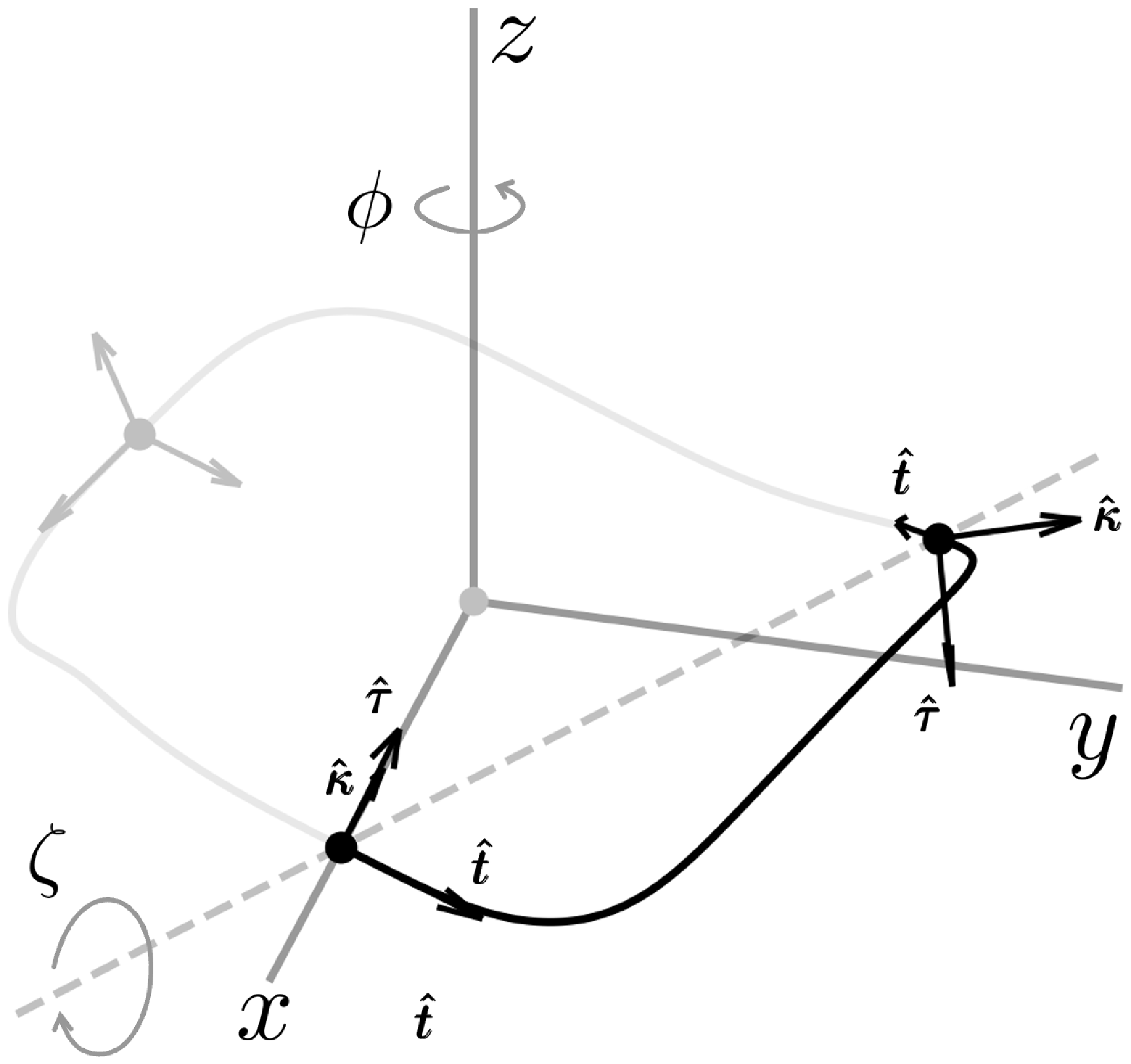


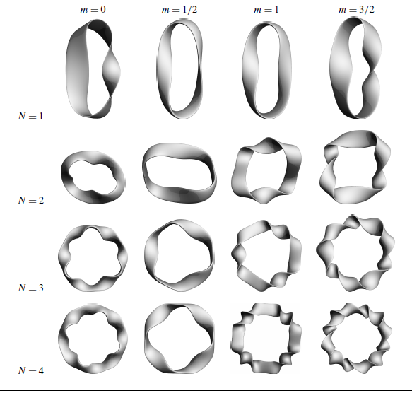


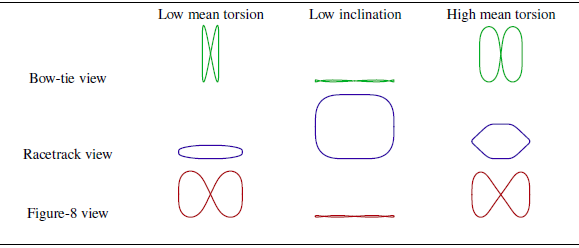


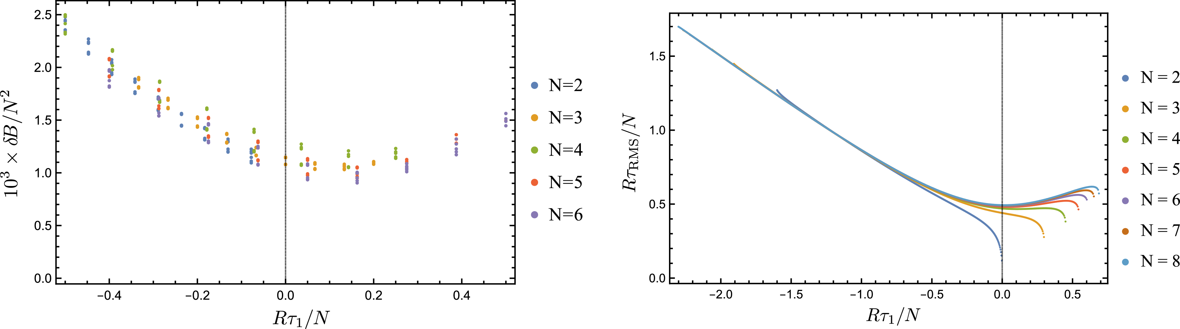


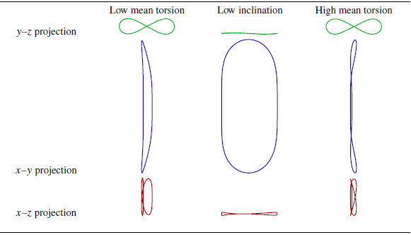


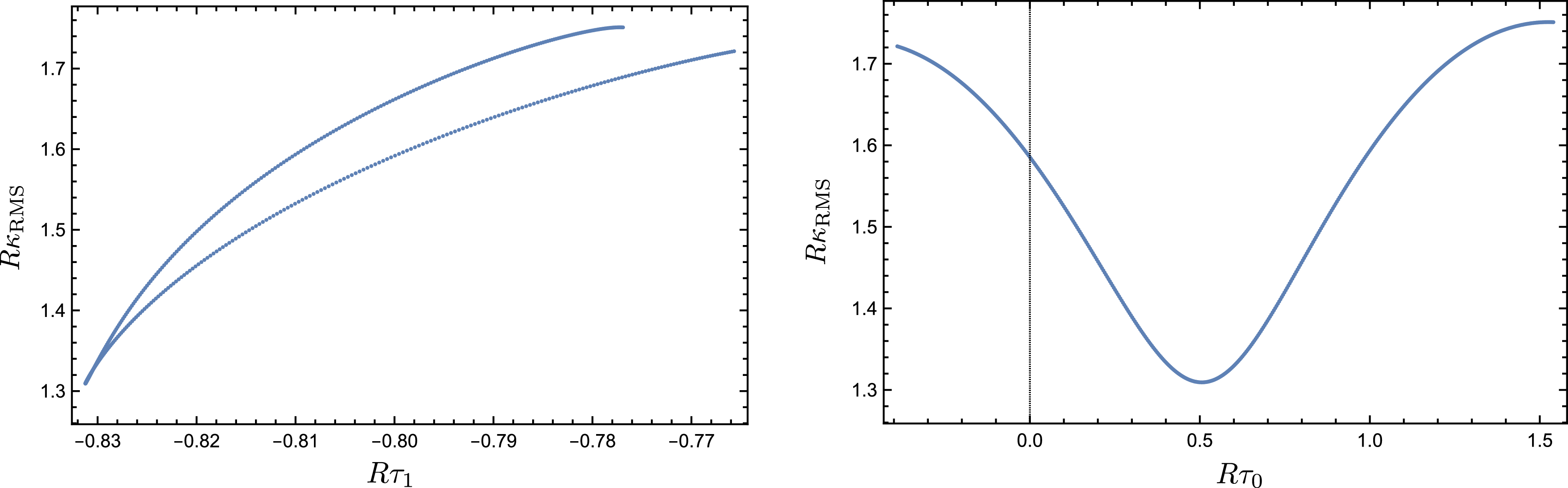


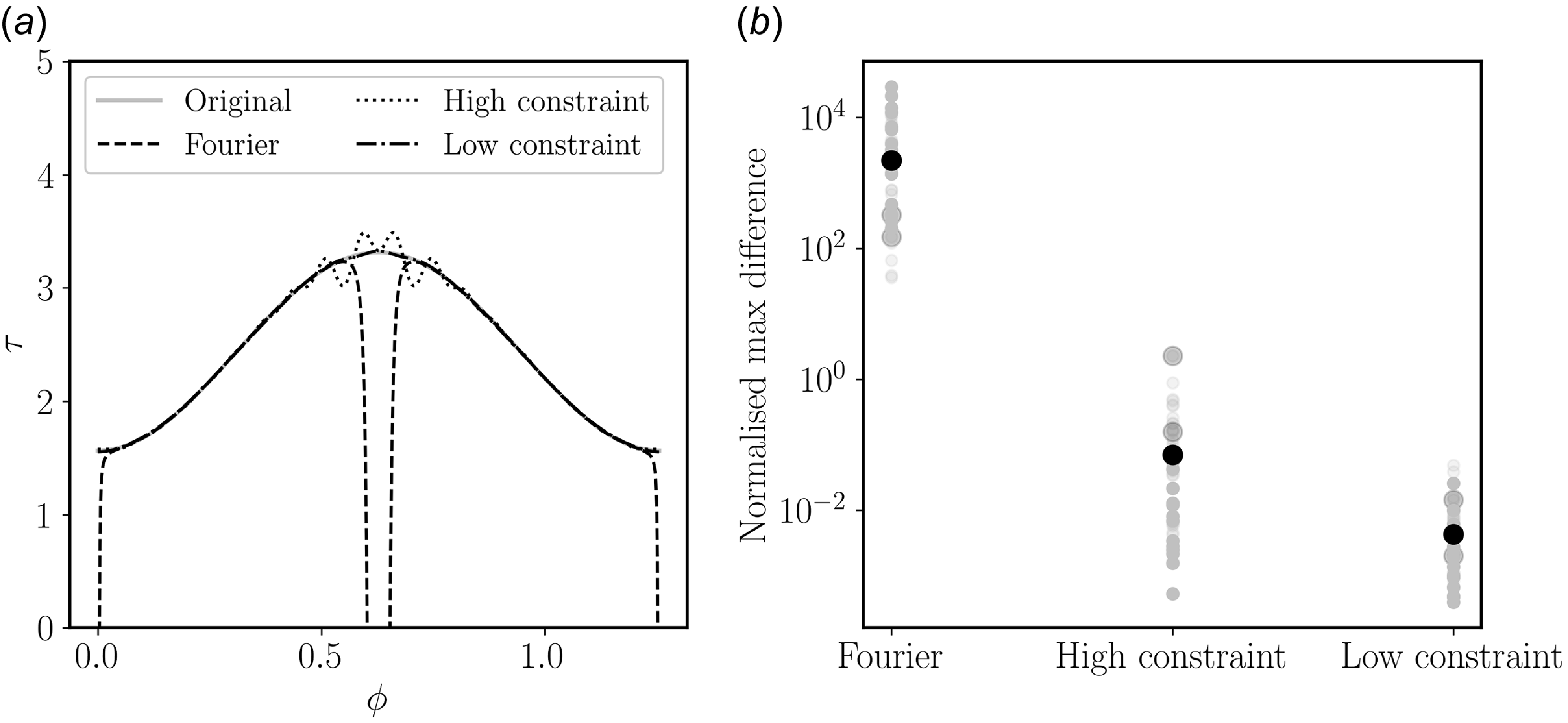


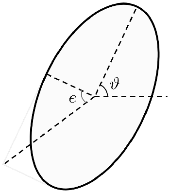


 Open access