2.1 Sea-ice dynamics in a continuum framework

Traditional continuum models for sea-ice dynamics solve the momentum equation for ice mass per unit area (m) as it flows through a fixed Eulerian mesh driven by winds and ocean currents. Here we used CICE, the Los Alamos Sea Ice Model employed by several Earth System Models (CICE Consortium, 2021). It solves the following 2-D momentum equation obtained by integrating the 3-D equation in the vertical direction through ice thickness (Hunke and Dukowicz, Reference Hunke and Dukowicz1997):

(1)$$m\displaystyle{{\partial {\boldsymbol u}} \over {\partial t}} = \nabla \cdot \sigma + {\boldsymbol \tau }_{\rm a} + {\boldsymbol \tau }_{\rm w}-\hat{{\boldsymbol k}} \times mf\,{\boldsymbol u}-mg\nabla H_{\rm o}$$

Here, u is the ice velocity, σ _ij is the internal stress tensor and τ_a and τ_w are the wind and ocean stresses, respectively. The two last terms on the right-hand side are stresses due to Coriolis effects and the sea surface slope. The ocean stress, which is tangential to the ice, is given by

(2)$${\boldsymbol \tau }_{\rm w} = C_{\rm w}\rho _{\rm w}\vert {{\boldsymbol U}_{\rm w}-{\boldsymbol u}} \vert [ {( {{\boldsymbol U}_{\rm w}-{\boldsymbol u}} ) \cos \theta + \hat{{\boldsymbol k}} \times ( {{\boldsymbol U}_{\rm w}-{\boldsymbol u}} ) \sin \theta } ] $$

where ρ _w, C _w and U_w are water density, drag coefficient and the current velocity, respectively; $\hat{{\boldsymbol k}}$ is the vertical unit vector and θ is the turning angle between geostrophic and surface currents. The turning angle is necessary if the top ocean model layers are not able to resolve the Ekman spiral in the boundary layer. If the top layer is sufficiently thin compared to the typical depth of the Ekman spiral, then θ = 0 is a good approximation. Here, as in CICE Consortium (2021), we assume that the top layer is thin enough. Similarly, the wind stress can be expressed via surface wind velocity:

(3)$${\boldsymbol \tau }_{\rm a} = C_{\rm a}\rho _{\rm a}\vert {{\boldsymbol U}_{\rm a}} \vert {\boldsymbol U}_{\rm a}$$

where ρ _a and C _a are air density and drag coefficient, respectively; and U_a is the wind velocity at 10 m.

CICE discretises the momentum equation in time and then solves it, utilising, for example, the elastic-viscous-plastic ice dynamics scheme (Hunke and Dukowicz, Reference Hunke and Dukowicz1997). In this scheme, σ _ij is determined from a regularised version of the VP constitutive law, which treats the ice pack as a visco-plastic material that flows plastically under typical stress conditions but behaves as a linear viscous fluid where strain rates are small. At each integration time step (typically, every hour or so), CICE finds velocity u and provides various data including but not limited to ice-drift direction, velocity, concentration and thickness. These parameters can serve as initial and boundary conditions for a nested DEM, as described in Section 2.3.

In our implementation, we used CICE with a mesh of 1° as illustrated in Figure 2. This resolution suffices for integration with the 100 × 100 km² DEM domain considered here.

2.2 Discrete element model

The utilised DEM solves the 3-D rigid-body equations of motion with the same force components as on the right-hand side of Eqn (1). However, since the icefield is now discrete (consisting of convex polyhedra), contact forces between rigid floes need to be modelled instead of the internal stress tensor in Eqn (1), and the fluid forces need to be integrated over the surfaces of the floes. Further, the force term due to the sea surface slope is neglected, as its effect is typically minor compared to the remaining terms (Leppäranta, Reference Leppäranta2011).

We employed a so-called non-smooth DEM formulated on the level of velocities and impulses, which contrasts with the traditional models formulated upon acceleration and forces. The comparative advantage of the current DEM is its efficiency in resolving a large number of contacts between interacting floes which may involve Coulomb friction and ice crushing (van den Berg and others, Reference van den Berg, Lubbad and Løset2018). Various analytical solutions for ice fracture due to interaction with icebreaking vessels have been implemented in this DEM. These solutions have been used to model icebreaker performance in ice management operations (e.g. Lubbad and others, Reference Lubbad, Løset, Lu, Tsarau and van den Berg2018). However, we cannot apply these analytical solutions for sea-ice fracture in our large-scale model, since they have been developed specifically for ice–structure interactions, which typically occur within the length of a ship, and may not be valid at larger scales. Thus, in our DEM simulations here, the ice floes cannot break.

Sea ice often undergoes fracturing processes, wherein ice floes crack or break into fragments or pieces. This can result from a variety of forces, such as tension, compression or shear forces. Although our present model cannot accurately describe the physics of ice fracture, it can be parameterised to predict local deformations of an icefield due to, for example, floe crushing and rafting. In this context, crushing refers to a specific type of fracturing process in which ice is subjected to mechanical compression that breaks it into smaller pieces or causes it to deform. For instance, when two ice floes interact, they may compact or shatter under pressure, resulting in the formation of small ice fragments at the contact zone. While our model does not simulate these small ice fragments, it allows the two floes to penetrate each other within the crushed volume and restore their shapes upon separation. The overlap volume of two interacting ice floes in the numerical simulation represents crushed ice. Figure 1 helps to illustrate this assumption.

Figure 1.

Overlap volume of two interacting floes represents crushed ice in the model of van den Berg and others (Reference van den Berg, Lubbad and Løset2018). For clarity, a 2-D sketch is shown here, but the algorithm is implemented fully in 3-D.

The contact model for floe–floe interaction is developed by van den Berg and others (Reference van den Berg, Lubbad and Løset2018) based on the assumption that local ice crushing will occur. In this model, ice crushing is represented by floe overlap (Fig. 1), and the corresponding restoring forces are calculated using exact contact geometries and material properties of interacting floes. Supported by experiments, van den Berg and others (Reference van den Berg, Lubbad and Løset2018) assumed constant energy dissipation per crushed volume or crushing specific energy (CSE). The latter is the amount of energy needed to crush a unit volume of ice, which can be equivalently expressed in J m⁻³ or Pa. The assumption of a constant CSE is equivalent to a constant crushing pressure (or plastic limit stress) during indentation, which is used to calculate the contact force when crushing starts:

(4)$$F_{{\rm cr}} = A_{{\rm proj}}\cdot {\rm CSE}$$

where F _cr is the limit of contact force above which crushing occurs, A _proj is the contact projected area and CSE is the crushing specific energy of sea ice. Below F _cr, the contact force is calculated such that the floes' relative velocity in the normal direction of their contact interface remains zero, or the force is zero in the case of separating floes. Additionally, there are tangential contact forces modelled according to the Coulomb friction law (for details, see van den Berg and others, Reference van den Berg, Lubbad and Løset2018).

Using this contact model and replacing CSE in Eqn (4) with a tuning parameter for floe ice strength, which may be different from its crushing specific energy, allows us to approximately model various scenarios involving floe rafting, ridging and crushing as plastic deformations of overlapping floes in our DEM. The values of this and other parameters used to model ice dynamics in this paper are given in Table 1.

Table 1.

Standard parameters used to model ice dynamics

2.3 Embedding DEM inside a larger sea-ice model

In our current approach, the embedded DEM was implemented to run in parallel with CICE. However, instead of the latter, any alternative tool for predicting large-scale sea-ice motion may be used, as there is currently no coupling between the models. Here, the embedded DEM domain is initially square with four linear boundaries enclosing discrete ice floes. The boundaries are rigid but can move independently from each other according to interpolated ice-drift velocities predicted by the continuum model (or other tools) in its own computational mesh nodes (Fig. 2). As these boundaries drift, they may confine the floes inside, such that no flux of ice through the boundaries is allowed. Thereby, the DEM domain can deform from its initial state while moving over the fixed-continuum model mesh. Note that there is no feedback passed from the DEM into the continuum model in our current approach.

Figure 2.

Fixed grid of the continuum model showing in colour an example of ice velocities predicted by CICE (left) and the nested boundaries of the DEM domain northeast of Svalbard with a close-up (right) illustrating how the DEM boundaries can move over the fixed grid. Two islands, Kvit and Victoria, may be located within the DEM domain as it moves and possibly deforms.

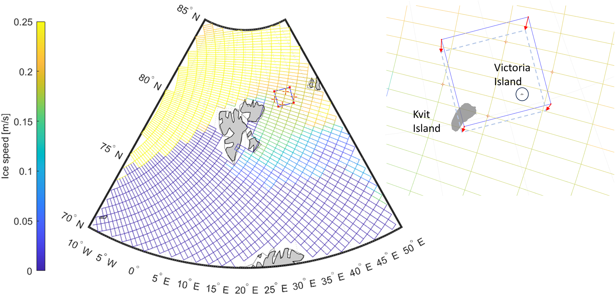
The dynamics within the DEM domain are computed based on atmosphere and ocean forcing data (as in Section 3.3), which may have higher temporal and spatial resolutions than the forcing data of the continuum model. The domain size of the adopted DEM in our applications is ~100 km, and the timescales can range from a fraction of a second up to a few days. The resolution of input data must be sufficient to resolve studied processes at these scales. As the duration of our simulations here is ~25 h, no thermodynamic processes are modelled within the DEM domain. Further specific details on the forcing data, boundary conditions, initialisation and execution of the model used in our analysis are given in Section 3.

3.1 Satellite imagery of the study site

The study site, which is the region where sea-ice drift is modelled and analysed in this paper, was chosen primarily based on data availability, including satellite optical imagery. We chose the Barents Sea because we also have our own observations and experience from various field experiments in this region (e.g. Tsarau and others, Reference Tsarau, Shestov and Løset2017). An interesting region was found using Sentinel-2 satellite imagery, covering the area northeast of Svalbard between Kvit Island and Victoria Island (see Fig. 2) with three successive images taken between 12.06 UTC on 15 April and 13.17 UTC on 16 April 2016 (Fig. 3).

Figure 3.

Sentinel-2 optical imagery of the same area northeast of Svalbard at 12.06 and 13.47 UTC on 15 April and at 13.17 UTC on 16 April 2016 (left to right) with Kvit Island and Victoria Island highlighted. The black triangular regions in the southern parts of the images indicate missing data or the presence of clouds.

Source: https://dataspace.copernicus.eu/

Each of the images in Figure 3 depicts the same geographic region of ~100 × 100 km². The GPS coordinates of this square region in decimal degrees are [79.90, 32.18] (bottom left) and [81.01, 38.92] (top right). The images were captured by Sentinel-2 sensors in a visible spectral band with a spatial resolution of 10 m. More details on the Sentinel-2 mission, including sensor characteristics and collected data, are provided by Drusch and others (Reference Drusch2012). In this study, it is important that the optical images are nearly cloud-free, enabling the identification of distinct ice floes and island boundaries. The presence of the islands shown in Figure 3 makes the considered case particularly interesting for our modelling because landmasses can cause deformation in pack ice, for example, due to shear, possibly involving breaking, and opening and closing of cracks. The localisation of deformation is an important aspect in our analysis.

3.2 Image analysis

Image processing techniques were employed in this paper to provide our DEM with an initial configuration of ice floes corresponding to the icefield depicted in the first image in Figure 3 (taken at 12.06 UTC on 15 April 2016). We used a procedure that involves the identification of greyscale thresholds for ice floes, image segmentation resulting in regions of ice and water, and subsequently processing the identified floe boundaries and shapes. These steps are commonly employed in image analysis methods used for automatic detection of ice floes (see e.g. Zhang and others, Reference Zhang, Skjetne and Su2013; Zhang and Skjetne, Reference Zhang and Skjetne2015). However, based on our experience, not all these methods may be equally effective when processing large, high-resolution images of a densely packed icefield (as in our case). They may also require manual intervention when floe boundaries are poorly identified, which is typical for highly concentrated icefields.

We achieved a balance between accuracy and efficiency by employing the well-known watershed transform for image segmentation, as inspired by Zhang and others (Reference Zhang, Skjetne and Su2013), preceded by the distance transform of the binary (ice-water) image. To prevent over-segmentation, we filtered out any shallow minima that might have resulted from the distance transform before applying the watershed segmentation algorithm. We further applied automatic geometric operations, such as convex hull, trimming and union, to the resulting segments, creating connected convex polygons that approximate the ice floes seen in Figure 3. This procedure simplifies any meanderings of the boundaries (see Fig. 4), preserving the overall shape of the floe, as long as it is nearly convex. Highly irregular, non-convex floes are divided into convex polygons to facilitate DEM modelling. Thus, the result of this image processing can be readily used in our DEM, as demonstrated in Figure 5. Here, a total of 10 737 ice floe with sizes ranging from 50 m to 16 km was modelled.

Figure 4.

Result of image segmentation (left) and a close-up view of the ice floes approximated by convex polygons (right).

Figure 5.

Icefield in the DEM represented by a total of 10 737 ice floes. The islands are shown in red.

Ice-drift fields can also be extracted from satellite imagery using feature tracking techniques. For instance, Itkin and others (Reference Itkin2018) used ridge sails in sea-ice surface topography data obtained by an airborne laser scanner as virtual buoys to identify displacements and drift velocities. Here, we used distinct features, for example, small floes and leads appearing in successive images in Figure 3, as markers and matched them across the images, employing the Computer Vision Toolbox in MATLAB R2022a, to retrieve displacements. These displacements were further converted into drift vectors, which served as the basis for reconstructing the sea-ice drift fields. The identified vector fields of ice motion are presented in Section 4.1.

3.3 Data sources

Optical satellite imagery does not provide data in the ice-thickness space, which is also required to initialise 3-D floes (polyhedra) in the DEM. Here, we used ice-thickness data from CS2–SMOS product (Ricker and others, Reference Ricker2017). This product combines thickness estimates from the European Space Agency CryoSat-2 (CS2) altimeter for thick ice (Ricker and others, Reference Ricker, Hendricks, Helm, Skourup and Davidson2014) and from the Soil Moisture and Ocean Salinity satellite for thin ice (Tian-Kunze and others, Reference Tian-Kunze2014), providing data for Arctic-wide studies on the entire thickness range. In our region of interest, the weekly average ice thickness provided by CS2–SMOS was ~0.3–0.55 m for the period from 9 April until 15 April 2016. We found rafted floe ice in a similar thickness range in the MIZ further south (downstream) from this area 2–3 weeks later (Tsarau and others, Reference Tsarau, Shestov and Løset2017), supporting the validity of the above estimates. Unfortunately, CS2–SMOS does not provide data after 15 April (presumably, due to the melt season). Therefore, we used the ice thickness data from the week before but covering a larger region (extending towards the north, from where the ice was drifting). The area-weighted average ice thickness in this region was ~0.45 m, which was used as the floe thickness in the DEM (the same for all floes). If high-resolution ice-thickness data were available on 15 April 2016 and onwards, the model could be initialised with a more realistic thickness distribution.

After initialising an icefield in the nested model, the force terms in Eqn (1) need to be provided. For wind forcing, we utilised the 10 m wind data from the NORA3 reanalysis, a high-resolution numerical mesoscale weather simulation for the North Sea, the Norwegian Sea and parts of the Barents Sea downscaled from the state-of-the-art ERA5 reanalysis (Solbrekke and others, Reference Solbrekke, Sorteberg and Haakenstad2021). Hourly wind speeds and directions with 3 km horizontal resolution were obtained for our DEM.

We also used the Hybrid Coordinate Ocean Model (HYCOM), which provides 41-layer ocean data in a 1/12° global grid with an average spacing of 6.5 km (Chassignet and others, Reference Chassignet2009). The temporal resolution of the HYCOM non-tidal surface current is 3 h; however, we interpolated it and added a tidal component to update our DEM with hourly estimates of the total surface current. This was done due to the lack of hourly current data from 2016 including both tidal and non-tidal components resolved in the upper ocean layer.

The tidal component was predicted using the Arctic 2 km Tide Model (Arc2kmTM) developed by Howard and Padman (Reference Howard and Padman2021). This is a barotropic ocean tide model on a 2 × 2 km² polar stereographic grid, developed using the Regional Ocean Modelling System. Arc2kmTM consists of spatial grids of complex amplitude coefficients for sea surface height and depth-integrated currents for eight principal tidal constituents: four semidiurnal (M2, S2, K2, N2) and four diurnal (K1, O1, P1, Q1). Using the Arc2kmTM model and its bathymetry data in the relevant region (Fig. 6), we obtained depth-averaged tidal currents, which were simply added to the HYCOM current to obtain an approximation of the total current (Fig. 7). The mean values of both current components (together with the wind data) are summarised in Table 2.

Figure 6.

Bathymetry map overlaid on top of Sentinel-2 optical imagery of the icefield possibly indicating more open ice in shallow water. The satellite image was taken at 12.06 UTC on 15 April 2016.

Figure 7.

Scaled vectors of wind (left) and total current (right) from 12.06 until 13.47 UTC on 15 April (blue) and from 13.47 UTC on 15 April until 13.17 UTC on 16 April 2016 (red) with Sentinel-2 imagery of the area in the background.

Table 2.

Mean wind and current data

All directions are measured from north, positive clockwise (e.g. drift towards the east is 90°).

3.4 Simulation procedures

The developed nested model was executed in different testing modes, which differed mainly in the way the DEM boundary conditions were provided. As presented in Section 2, a trial set-up of the nested model was developed to run in parallel with CICE; however, any alternative tool for predicting large-scale sea-ice motion may be used. We considered this trial set-up, running both models, CICE and DEM, locally to make sure that the nested DEM concept is feasible. A standard version of CICE 6.4.0 on a 1° global grid was utilised here following the preparation and execution steps described by CICE Consortium (2021). The DEM set-up was as described in Section 2.2, with its own wind and ocean data as presented in Section 3.3. Both models have their own numerical integration schemes with different time stepping. A typical time step in CICE is ~1 h, while the DEM solves sea-ice dynamics at 0.2 s intervals. The larger of these two time steps was used as a communication interval to update the boundary conditions in the DEM with CICE data. Communication with the DEM was implemented via the TCP/IP network interface, allowing data exchange between different machines on the network. In this simulation, we were only sending data from CICE to the DEM; however, it may also be possible updating some data fields in CICE based on DEM predictions (e.g. information about ice concentration, leads and floe-size distribution) for coupling. Fully coupled simulations may be considered in future. Since CICE with its large time step may run much faster than the DEM, the predicted continuum ice velocities were stored in a buffer. From there, the DEM TCP/IP module was reading the hourly data, interpolating it to the DEM boundaries, and then updating the DEM boundary conditions. This simulation is depicted in Figure 2, where the DEM domain moves over the 1° grid with velocities predicted by CICE. Here, the centres of the rigid DEM boundaries move with ice velocities in the nearest nodes of CICE.

To compare the DEM performance against observed data and investigate the effect of boundary conditions, we considered another simulation procedure with prescribed boundary velocities. To avoid unnecessary efforts validating CICE simulations against satellite observations and rather focus on the performance of the DEM, we obtained possible sets of boundary conditions directly from the available satellite images. This was done based on the same feature tracking technique described in Section 4.1. The results are presented in Table 3 providing time-dependent (N1) and constant (N2) boundary velocities, which are the same for the northern, southern, eastern and western boundaries in both cases here. Additionally, we implemented a set-up with no confinement along the boundaries (N3), which means no internal force was prescribed on the floes at the boundaries. We used different boundary conditions in our numerical experiments to investigate how the accuracy and different update frequencies (constant vs variable) of boundary velocities impact the accuracy of DEM simulations. Among the sets of boundary conditions presented in Table 1, N1 is considered the most accurate, while N3 is an extreme simplification.

Table 3.

Boundary conditions used in the DEM simulations

In N1 and N2, ice-drift velocities obtained from Sentinel-2 images were prescribed on the rigid DEM boundaries (the same for the northern, southern, eastern and western boundaries here). In N3, no rigid boundaries were modelled representing a scenario with no confinement.

These sets of boundary conditions (Table 3) were used to update our DEM in the simulations presented in Section 4. Otherwise, the procedure for executing the model was the same as described above for concurrent CICE-DEM simulations. Standard (or rather typical) parameters for modelling ice dynamics were used, as listed in Table 1.

In all our simulations here, the ice floes were generated using the satellite image taken at 12.06 UTC on 15 April (in Fig. 3) as described in Section 3.2. For practical reasons, all floes were initialised with the velocities of the current in the DEM. In some scenarios, more accurate initial conditions could potentially be obtained, for example, by interpolating the DEM boundary velocities. In simulations with CICE, continuum velocity predictions could be used. However, we did not explore these options.