


1. Introduction
This paper concerns weak, freely decaying, homogeneous turbulence subject to rotation, represented by ${\varOmega}$
, and stable stratification, expressed by a constant Brunt–Vaisala frequency,
${\varOmega}$
, and stable stratification, expressed by a constant Brunt–Vaisala frequency, $N$
. The approach used is a spectral one, i.e. based on Fourier transforms, and a general overview of homogeneous turbulence with this viewpoint in mind can be found in the book by Sagaut & Cambon (Reference Sagaut and Cambon2018). By weak turbulence, we mean that either the Rossby number,
$N$
. The approach used is a spectral one, i.e. based on Fourier transforms, and a general overview of homogeneous turbulence with this viewpoint in mind can be found in the book by Sagaut & Cambon (Reference Sagaut and Cambon2018). By weak turbulence, we mean that either the Rossby number, $u'/{\varOmega} L$
, or Froude number,
$u'/{\varOmega} L$
, or Froude number, $u'/NL$
, is small, where
$u'/NL$
, is small, where $u'$
and
$u'$
and $L$
are measures of the turbulent velocity and the size of its large scales.
$L$
are measures of the turbulent velocity and the size of its large scales.
This article uses the formulation of Scott & Cambon (Reference Scott and Cambon2024) (henceforth referred to as [I]) as a basis. We should note that the restriction to a small wave/non-propagating (NP) amplitude ratio of [I] was lifted in Scott (Reference Scott2025). As in [I], the flow is expressed as a linear combination of modes, each a solution of the governing equations without nonlinearity or visco-diffusion, which form a complete set capable of representing general solenoidal velocity fields. The modes are of two types: oscillatory ones which represent inertial/gravity waves and time-independent ones, referred to as NP because they have zero frequency, hence zero group velocity. It was shown in [I] that, for weak turbulence, the NP component of the flow decouples from the wave one at leading order and can thus be studied on its own, which is what we do here.
As was noted in [I] and demonstrated in this article, the governing equations of the NP component of weak turbulence are equivalent to the three-dimensional, quasi-geostrophic (QG) approximation, which is widely used in geophysical applications and has a long history. Thus, the present work applies directly to QG turbulence. The QG approximation was first proposed by Charney (Reference Charney1948), whose later publication, Charney (Reference Charney1971) (henceforth referred to as [II]), is perhaps the most influential article in the area of QG turbulence and will be referred to on multiple occasions in what follows. Although now rather dated, the review by Rhines (Reference Rhines1979) provides an overview of QG turbulence. Since the parameter $\beta =2{\varOmega} /N$
is usually small for atmospheric and oceanic flows, such smallness is sometimes implicit in geophysical studies, whereas small
$\beta =2{\varOmega} /N$
is usually small for atmospheric and oceanic flows, such smallness is sometimes implicit in geophysical studies, whereas small $\beta$
is not supposed here. Note that the notation
$\beta$
is not supposed here. Note that the notation $\beta =2{\varOmega} /N$
, used in the present article, has no connection with the geophysical
$\beta =2{\varOmega} /N$
, used in the present article, has no connection with the geophysical $\beta$
-plane, used to approximate a spherical Earth. There is no
$\beta$
-plane, used to approximate a spherical Earth. There is no $\beta$
-plane effect here.
$\beta$
-plane effect here.
The work in [II] drew a formal analogy between QG turbulence and the physically different problem of two-dimensional turbulence (without rotation or stratification). Two-dimensional turbulence has been the subject of much work (see the review by Boffetta & Ecke (Reference Boffetta and Ecke2012)). Perhaps the most important conclusion is that there are two cascades. Energy goes from small to large scales, while enstrophy (one half the mean squared vorticity) is transferred in the opposite direction. In the isotropic case, each cascade is associated with a power law for the energy spectrum: $k^{-5/3}$
for the energy cascade and
$k^{-5/3}$
for the energy cascade and $k^{-3}$
for enstrophy, where
$k^{-3}$
for enstrophy, where $k$
is the wavenumber. Thus, if external forcing is applied at a particular wavenumber and the Reynolds number is large, one expects
$k$
is the wavenumber. Thus, if external forcing is applied at a particular wavenumber and the Reynolds number is large, one expects $k^{-5/3}$
below that wavenumber and
$k^{-5/3}$
below that wavenumber and $k^{-3}$
above it. Transfer of enstrophy towards smaller scales eventually encounters viscosity, producing a range of
$k^{-3}$
above it. Transfer of enstrophy towards smaller scales eventually encounters viscosity, producing a range of $k$
above the
$k$
above the $k^{-3}$
one in which the enstrophy flux is dissipated and the spectrum falls off rapidly. For freely decaying turbulence, the enstrophy cascade leads to a
$k^{-3}$
one in which the enstrophy flux is dissipated and the spectrum falls off rapidly. For freely decaying turbulence, the enstrophy cascade leads to a $k^{-3}$
inertial range, while the energy cascade produces growth in the size of the large scales. Given that the energy transfer is towards the larger scales, one expects that energy dissipation is small at large Reynolds number, in principle going to zero at infinite Reynolds number, hence energy conservation in the inviscid case.
$k^{-3}$
inertial range, while the energy cascade produces growth in the size of the large scales. Given that the energy transfer is towards the larger scales, one expects that energy dissipation is small at large Reynolds number, in principle going to zero at infinite Reynolds number, hence energy conservation in the inviscid case.
For QG turbulence, which is three-dimensional, [II] suggested that a quantity known as potential enstrophy plays much the same role in the QG problem as enstrophy does in the two-dimensional one. As a result, he proposed two cascades, with energy going towards larger scales and potential enstrophy towards smaller ones. The work in [II] concluded that energy should be nearly conserved and that the energy spectrum should have an inertial range in which it behaves as $k^{-3}$
. He also proposed that the energy distribution in spectral space is isotropic when expressed using coordinates in which the vertical wavenumber is multiplied by
$k^{-3}$
. He also proposed that the energy distribution in spectral space is isotropic when expressed using coordinates in which the vertical wavenumber is multiplied by $\beta$
. Note that such ‘Charney isotropy’ does not imply isotropy in the usual sense unless
$\beta$
. Note that such ‘Charney isotropy’ does not imply isotropy in the usual sense unless $\beta =1$
. Thus, when
$\beta =1$
. Thus, when $\beta \,{\lt}\, 1$
, Charney isotropy leads to a vertically elongated energy distribution, while, for
$\beta \,{\lt}\, 1$
, Charney isotropy leads to a vertically elongated energy distribution, while, for $\beta \,{\gt}\, 1$
, the predicted distribution extends further in the horizontal than in the vertical direction. Charney isotropy makes the energy distribution axisymmetric and implies the result that the average kinetic energy should be twice the potential one, a condition sometimes known as Charney equipartition.
$\beta \,{\gt}\, 1$
, the predicted distribution extends further in the horizontal than in the vertical direction. Charney isotropy makes the energy distribution axisymmetric and implies the result that the average kinetic energy should be twice the potential one, a condition sometimes known as Charney equipartition.
Charney’s suggestion of isotropy was supported by the numerical simulations of QG turbulence by Hua & Haidvogel (Reference Hua and Haidvogel1986) and McWilliams (Reference McWilliams1989), of whom the latter also demonstrated the similarities of QG and two-dimensional turbulence regarding cascades and their directions. More recent simulations by Vallgren & Lindborg (Reference Vallgren and Lindborg2010) also support the predictions of [II]. As we shall see, our results agree with most of the proposals of [II], but not isotropy. This is one of the notable conclusions of this article. Another being self-similarity of the time evolution of the distribution of energy in spectral space at large enough times and away from the vertical axis.
The article by Smith & Waleffe (Reference Smith and Waleffe2002) is representative of studies of rotating/stratified turbulence using full direct numerical simulation. It is based on the Boussinesq equations, rather than the QG ones used here and considers forced turbulence, rather the freely decaying case which is the subject of this article. Only limited comparisons with [II] are made.
Although we focus on energy, we should observe that QG flows are rich in structures such as vortices, and the statistics of these have been explored by, for instance, McWilliams (Reference McWilliams1990), McWilliams, Weiss & Yavneh (Reference McWilliams, Weiss and Yavneh1999), Dritschel, de la Torre Juarez & Ambaum (Reference Dritschel, de la Torre Juarez and Ambaum1999), von Hardenberg et al. (Reference von Hardenberg, McWilliams, Provenzale, Shchepetkin and Weiss2000) and Reinaud, Dritschel & Koudella (Reference Reinaud, Dritschel and Koudella2003). However, in this article we concentrate on the energy and its distribution in spectral space.
This paper is organised as follows. Section 2 describes the theoretical basis, the weak-turbulence limit and its relationship with the QG approximation and a transformation of variables which essentially removes the parameter $\beta$
from consideration. Finally, § 3 gives numerical results.
$\beta$
from consideration. Finally, § 3 gives numerical results.
2. Formulation
Consider freely decaying homogeneous turbulence in an unbounded, incompressible, rotating, stably stratified fluid having constant density, constant Brunt–Vaisala frequency, $N$
, and constant rotation vector,
$N$
, and constant rotation vector, $\boldsymbol{\varOmega }$
, which is supposed parallel to gravity and has unit vector
$\boldsymbol{\varOmega }$
, which is supposed parallel to gravity and has unit vector $\boldsymbol{e}=\boldsymbol{\varOmega }/{\varOmega}$
, where
$\boldsymbol{e}=\boldsymbol{\varOmega }/{\varOmega}$
, where ${\varOmega} =| \boldsymbol{\varOmega }|$
. Henceforth, spatial coordinates, time and velocity are non-dimensionalised using
${\varOmega} =| \boldsymbol{\varOmega }|$
. Henceforth, spatial coordinates, time and velocity are non-dimensionalised using $L , (N^{2}+4{\varOmega} ^{2})^{-1/2}$
and
$L , (N^{2}+4{\varOmega} ^{2})^{-1/2}$
and $L(N^{2}+4{\varOmega} ^{2})^{1/2}$
, where
$L(N^{2}+4{\varOmega} ^{2})^{1/2}$
, where $L$
is a length scale characterising the large scales of the initial turbulence.
$L$
is a length scale characterising the large scales of the initial turbulence.
2.1. Analytical background
Using a rotating frame of reference and Cartesian coordinates, as well as the summation convention, the non-dimensional Boussinesq equations of motion are
 \begin{align}&\qquad\qquad\qquad\qquad\qquad\,\, \frac{\partial u_{i}}{\partial x_{i}}=0 ,\end{align}
where $\varepsilon _{ijk}$
is the alternating tensor,
$\varepsilon _{ijk}$
is the alternating tensor, ![]() and
and ![]() . Furthermore,
. Furthermore, $D_{u}=\nu (N^{2}+4{\varOmega} ^{2})^{-1/2}L^{-2}$
and
$D_{u}=\nu (N^{2}+4{\varOmega} ^{2})^{-1/2}L^{-2}$
and $D_{\eta }=\kappa (N^{2}+4{\varOmega} ^{2})^{-1/2}L^{-2}$
, where
$D_{\eta }=\kappa (N^{2}+4{\varOmega} ^{2})^{-1/2}L^{-2}$
, where $\nu$
is the kinematic viscosity and
$\nu$
is the kinematic viscosity and $\kappa$
the diffusivity associated with the buoyancy variable
$\kappa$
the diffusivity associated with the buoyancy variable $\eta$
. Note that
$\eta$
. Note that ![]() and
and ![]() , where
, where ![]() . Thus, the non-dimensional governing equations, (2.1)–(2.3), only depend on the parameters
. Thus, the non-dimensional governing equations, (2.1)–(2.3), only depend on the parameters $\beta , D_{u}$
and
$\beta , D_{u}$
and $D_{\eta }$
. For simplicity’s sake,
$D_{\eta }$
. For simplicity’s sake, ![]() are denoted
are denoted ${\varOmega} , N$
in what follows. Because we will only be working with non-dimensional quantities, this should not lead to confusion. Note that the right-hand sides of (2.1) and (2.3) express nonlinearity, viscosity and diffusion. The visco-diffusive terms dissipate energy.
${\varOmega} , N$
in what follows. Because we will only be working with non-dimensional quantities, this should not lead to confusion. Note that the right-hand sides of (2.1) and (2.3) express nonlinearity, viscosity and diffusion. The visco-diffusive terms dissipate energy.
As described in [I], in the absence of nonlinearity and visco-diffusion, (2.1)–(2.3) have particular solutions, referred to as modes, which are indexed by an integer $s=0,\pm 1$
and a wave vector
$s=0,\pm 1$
and a wave vector $\boldsymbol{k}$
. Modes have the velocity and buoyancy variable
$\boldsymbol{k}$
. Modes have the velocity and buoyancy variable
 \begin{align}u_{i} & = v_{i}^{(s)}(\boldsymbol{k})\exp (i(\boldsymbol{k}\boldsymbol{\cdot} \boldsymbol{x}-s\omega (\boldsymbol{k})t)),\\[-12pt]\nonumber\end{align}
 \begin{align}\eta & = \eta ^{(s)}(\boldsymbol{k})\exp (i(\boldsymbol{k}\boldsymbol{\cdot} \boldsymbol{x}-s\omega (\boldsymbol{k})t)) ,\end{align}
where the notation $\boldsymbol{\cdot}$
represents a scalar product,
$\boldsymbol{\cdot}$
represents a scalar product,
 \begin{equation} \omega(\boldsymbol{k})=(N^{2}\sin ^{2}\theta +{\varOmega} ^{2}\cos ^{2}\theta )^{1/2} ,\end{equation}
where $\theta$
is the angle between
$\theta$
is the angle between $\boldsymbol{k}$
and the rotation vector and
$\boldsymbol{k}$
and the rotation vector and $v_{i}^{(s)} , \eta ^{(s)}$
are given by (I.2.12)–(I.2.15) (where, here and henceforth, (I.x.y) refers to equation (x.y) of [I]).
$v_{i}^{(s)} , \eta ^{(s)}$
are given by (I.2.12)–(I.2.15) (where, here and henceforth, (I.x.y) refers to equation (x.y) of [I]).
Although modes do not allow for nonlinearity or visco-diffusion, they form a complete set for $u_{i}(\boldsymbol{x}) , \eta (\boldsymbol{x})$
satisfying (2.2). Thus, the flow can be expressed at any given time as
$u_{i}(\boldsymbol{x}) , \eta (\boldsymbol{x})$
satisfying (2.2). Thus, the flow can be expressed at any given time as
 \begin{equation} u_{i}=\sum _{s=0,\pm 1}u_{i,s} ,\quad \eta =\sum _{s=0,\pm 1}\eta _{s} ,\end{equation}
where
 \begin{align}u_{i,s}&=\int\! a_{s}(\boldsymbol{k},t)v_{i}^{(s)}(\boldsymbol{k})\exp (i(\boldsymbol{k}\boldsymbol{\cdot} \boldsymbol{x}-s\omega (\boldsymbol{k})t))d^{3}\boldsymbol{k},\\[-12pt]\nonumber\end{align}
 \begin{align}\eta _{s}&=\int\! a_{s}(\boldsymbol{k},t)\eta ^{(s)}(\boldsymbol{k})\exp (i(\boldsymbol{k}\boldsymbol{\cdot} \boldsymbol{x}-s\omega (\boldsymbol{k})t))d^{3}\boldsymbol{k} ,\end{align}
and $a_{s}$
are the mode amplitudes at time
$a_{s}$
are the mode amplitudes at time $t$
. The
$t$
. The $a_{s}$
evolve in time due to nonlinearity and visco-diffusion.
$a_{s}$
evolve in time due to nonlinearity and visco-diffusion.
Equations (2.7)–(2.9) express the flow as a linear combination of modes indexed by $s=0,\pm 1$
and the wave vector
$s=0,\pm 1$
and the wave vector $\boldsymbol{k}$
, each mode being a solution of the governing equations without visco-diffusion and nonlinearity of the form
$\boldsymbol{k}$
, each mode being a solution of the governing equations without visco-diffusion and nonlinearity of the form $\exp (i(\boldsymbol{k}\boldsymbol{\cdot} \boldsymbol{x}-s\omega (\boldsymbol{k})t))$
. The modes with
$\exp (i(\boldsymbol{k}\boldsymbol{\cdot} \boldsymbol{x}-s\omega (\boldsymbol{k})t))$
. The modes with $s=\pm 1$
are inertial-gravity waves, whose dispersion relation is (2.6). The non-dimensionalisation of time makes the period of oscillation of such waves of order
$s=\pm 1$
are inertial-gravity waves, whose dispersion relation is (2.6). The non-dimensionalisation of time makes the period of oscillation of such waves of order $1$
. The mode
$1$
. The mode $s=0$
has zero frequency, hence zero group velocity. Thus, the corresponding component of the flow is indeed non-propagating, hence its designation by NP. As in [I], since
$s=0$
has zero frequency, hence zero group velocity. Thus, the corresponding component of the flow is indeed non-propagating, hence its designation by NP. As in [I], since $u_{i}$
and
$u_{i}$
and $\eta$
are real,
$\eta$
are real, $a_{s}(-\boldsymbol{k})=a_{-s}^{*}(\boldsymbol{k})$
, where
$a_{s}(-\boldsymbol{k})=a_{-s}^{*}(\boldsymbol{k})$
, where $^{*}$
denotes complex conjugation. Using the identities
$^{*}$
denotes complex conjugation. Using the identities $v_{i}^{(s)}(-\boldsymbol{k})=v_{i}^{(-s)^{*}}(\boldsymbol{k}) , \eta ^{(s)}(-\boldsymbol{k})=\eta ^{(-s)^{*}}(\boldsymbol{k})$
and
$v_{i}^{(s)}(-\boldsymbol{k})=v_{i}^{(-s)^{*}}(\boldsymbol{k}) , \eta ^{(s)}(-\boldsymbol{k})=\eta ^{(-s)^{*}}(\boldsymbol{k})$
and $\omega (-\boldsymbol{k})=\omega (\boldsymbol{k})$
, (2.8) and (2.9) imply
$\omega (-\boldsymbol{k})=\omega (\boldsymbol{k})$
, (2.8) and (2.9) imply $u_{i,s}=u_{i,-s}^{*} , \eta _{s}=\eta _{-s}^{*}$
. Thus, the NP component, defined by
$u_{i,s}=u_{i,-s}^{*} , \eta _{s}=\eta _{-s}^{*}$
. Thus, the NP component, defined by $u_{i}^{\it{NP}}=u_{i,0}$
and
$u_{i}^{\it{NP}}=u_{i,0}$
and $\eta ^{\it{NP}}=\eta _{0}$
, is real, whereas
$\eta ^{\it{NP}}=\eta _{0}$
, is real, whereas $s=+1$
and
$s=+1$
and $s=-1$
provide conjugate contributions to (2.7), whose sum is the wave component and is also real.
$s=-1$
provide conjugate contributions to (2.7), whose sum is the wave component and is also real.
According to (I.2.26), the evolution of the modal amplitudes is described by
 \begin{equation} \frac{\partial a_{s}}{\partial t}=-ik_{j}(v_{i}^{(s)^{*}}\widetilde{\phantom{uu}{\kern-10pt}u_{i}u_{j}}+\eta ^{(s)^{*}}\widetilde{\phantom{\,}\eta u_{\!j}})\exp (is\omega t)-\sum _{\hat{s}=0,\pm 1}\! D_{s\hat{s}}\exp (i(s-\hat{s})\omega t)a_{\hat{s}} ,\end{equation}
where $s=0,\pm 1$
,
$s=0,\pm 1$
,
 \begin{equation} \tilde{f}(\boldsymbol{k})=\frac{1}{8\pi ^{3}}\int\! f(\boldsymbol{x})\exp (-i\boldsymbol{k}\boldsymbol{\cdot} \boldsymbol{x})d^{3}\boldsymbol{x} \end{equation}
defines spatial Fourier transformation and $D_{s\hat{s}}$
is the Hermitian, positive definite matrix given by (I.2.20) and which represents visco-diffusion.
$D_{s\hat{s}}$
is the Hermitian, positive definite matrix given by (I.2.20) and which represents visco-diffusion.
Since we want to study turbulent flow, a statistical ensemble of flow realisations is introduced, as well as ensemble averaging. The flow is assumed to have initial statistics which are homogeneous with respect to spatial translation, a property which is preserved by time evolution according to the governing equations, (2.1)–(2.3). The flow is also assumed to be initially of zero mean, i.e. $\overline{u_{i}}=0$
and
$\overline{u_{i}}=0$
and $\overline{\eta }=0$
, where the overbars denote ensemble averaging. Given homogeneity, this property is also preserved by (2.1)–(2.3). Here,
$\overline{\eta }=0$
, where the overbars denote ensemble averaging. Given homogeneity, this property is also preserved by (2.1)–(2.3). Here, $\overline{u_{i}}=0 , \overline{\eta }=0$
can be shown to imply
$\overline{u_{i}}=0 , \overline{\eta }=0$
can be shown to imply $\overline{a_{s}}=0$
and
$\overline{a_{s}}=0$
and $\overline{u_{i,s}}=\overline{\eta _{s}}=0$
. Thus,
$\overline{u_{i,s}}=\overline{\eta _{s}}=0$
. Thus, $a_{s}$
and both the wave and NP components of the flow have zero mean.
$a_{s}$
and both the wave and NP components of the flow have zero mean.
Given the statistical homogeneity of the flow, the second-order moments of the modal amplitudes have the form
 \begin{equation} \overline{a_{s}^{*}(\boldsymbol{k})a_{s'}(\boldsymbol{k}')}=A_{ss'}(\boldsymbol{k})\delta (\boldsymbol{k}-\boldsymbol{k}') ,\end{equation}
where $A_{ss'}$
is a Hermitian, positive semidefinite matrix, referred to as the spectral matrix. Since
$A_{ss'}$
is a Hermitian, positive semidefinite matrix, referred to as the spectral matrix. Since $a_{s}(-\boldsymbol{k})=a_{-s}^{*}(\boldsymbol{k}) , A_{ss'}(-\boldsymbol{k})=A_{-s',-s}(\boldsymbol{k})$
. The average non-dimensional energy per unit volume in physical space is
$a_{s}(-\boldsymbol{k})=a_{-s}^{*}(\boldsymbol{k}) , A_{ss'}(-\boldsymbol{k})=A_{-s',-s}(\boldsymbol{k})$
. The average non-dimensional energy per unit volume in physical space is
 \begin{equation} \underset{\it{Kinetic}}{\underbrace{\frac{1}{2}\overline{u_{i}u_{i}}}}+\underset{\it{Potential}}{\underbrace{\frac{1}{2}\overline{\eta ^{2}}}}=\int\! e(\boldsymbol{k})d^{3}\boldsymbol{k} ,\end{equation}
where
 \begin{equation} e(\boldsymbol{k})=\tfrac{1}{2}\sum _{s=0,\pm 1}\! A_{ss}(\boldsymbol{k}) \end{equation}
is the energy density in spectral space. Equation (2.14) indicates that the diagonal elements of $A_{ss'}$
yield the contribution,
$A_{ss'}$
yield the contribution, $A_{ss}/2$
, of mode
$A_{ss}/2$
, of mode $\boldsymbol{k} , s$
to the energy density. Given that
$\boldsymbol{k} , s$
to the energy density. Given that $A_{ss'}$
is Hermitian and positive semidefinite, the modal energy contribution is real and non-negative. The off-diagonal elements of
$A_{ss'}$
is Hermitian and positive semidefinite, the modal energy contribution is real and non-negative. The off-diagonal elements of $A_{ss'}$
can be complex and represent correlations between modes of different
$A_{ss'}$
can be complex and represent correlations between modes of different $s$
. The spectral energy density can be split into wave and NP contributions as
$s$
. The spectral energy density can be split into wave and NP contributions as $e=e_{W}+e_{\it{NP}}$
, where
$e=e_{W}+e_{\it{NP}}$
, where
 \begin{equation} e_{W}=\tfrac{1}{2}\sum _{s=\pm 1}A_{ss},\quad e_{\it{NP}}=\tfrac{1}{2}A_{00} .\end{equation}
Since $A_{ss'}(-\boldsymbol{k})=A_{-s',-s}(\boldsymbol{k}) , e_{W}(-\boldsymbol{k})=e_{W}(\boldsymbol{k})$
and
$A_{ss'}(-\boldsymbol{k})=A_{-s',-s}(\boldsymbol{k}) , e_{W}(-\boldsymbol{k})=e_{W}(\boldsymbol{k})$
and $e_{\it{NP}}(-\boldsymbol{k})=e_{\it{NP}}(\boldsymbol{k})$
. The NP contribution to the average energy per unit volume is
$e_{\it{NP}}(-\boldsymbol{k})=e_{\it{NP}}(\boldsymbol{k})$
. The NP contribution to the average energy per unit volume is
 \begin{equation} E_{\it{NP}}=\underset{\it{Kinetic}}{\underbrace{\frac{1}{2}\overline{u_{i}^{\it{NP}}u_{i}^{\it{NP}}}}}+\underset{\it{Potential}}{\underbrace{\frac{1}{2}\overline{\eta ^{N\!P^{2}}}}}=\int\! e_{\it{NP}}(\boldsymbol{k})d^{3}\boldsymbol{k} .\end{equation}
The subject of this article being the NP component of the flow, we note that
 \begin{align}v_{1}^{(0)}& =\frac{ik_{2}}{\big(k_{1}^{2}+k_{2}^{2}+\beta ^{2}k_{3}^{2}\big)^{1/2}},\quad v_{2}^{(0)}=-\frac{ik_{1}}{\big(k_{1}^{2}+k_{2}^{2}+\beta ^{2}k_{3}^{2}\big)^{1/2}},\quad v_{3}^{(0)}=0,\\[-12pt]\nonumber\end{align}
 \begin{align}\eta^{(0)}&=\frac{i\beta k_{3}}{\big(k_{1}^{2}+k_{2}^{2}+\beta ^{2}k_{3}^{2}\big)^{1/2}} \end{align}
follow from (I.2.12), (I.2.13), (I.2.15) and $\beta ={\varOmega} /N$
, where, here and henceforth,
$\beta ={\varOmega} /N$
, where, here and henceforth, $x_{1}$
and
$x_{1}$
and $x_{2}$
are horizontal coordinates, while
$x_{2}$
are horizontal coordinates, while $x_{3}$
is vertical (so
$x_{3}$
is vertical (so $\boldsymbol{e}=(0,0,1)$
). We also note that the NP mode damping coefficient is
$\boldsymbol{e}=(0,0,1)$
). We also note that the NP mode damping coefficient is
 \begin{equation} D_{00}=k^{2}\frac{D_{u}\big(k_{1}^{2}+k_{2}^{2}\big)+D_{\eta }\beta ^{2}k_{3}^{2}}{k_{1}^{2}+k_{2}^{2}+\beta ^{2}k_{3}^{2}} ,\end{equation}
according to (I.2.15) and (I.2.20), where $k=| \boldsymbol{k}|$
. Observe that (2.8) and (2.17) imply that the NP velocity,
$k=| \boldsymbol{k}|$
. Observe that (2.8) and (2.17) imply that the NP velocity, $u_{i}^{\it{NP}}=u_{i,0}$
, is horizontal and divergence free.
$u_{i}^{\it{NP}}=u_{i,0}$
, is horizontal and divergence free.
2.2. Weak turbulence and the QG approximation
From here on, we suppose that the turbulence is weak (small Rossby or Froude number). Given the temporal oscillations of the wave modes, it is shown in [I] (§ 3.1) that (2.10) with $s=0$
has the leading-order approximation
$s=0$
has the leading-order approximation
 \begin{equation} \frac{\partial a_{0}}{\partial t}+D_{00}a_{0}=-ik_{j}\Big(v_{i}^{(0)^{*}}\widetilde{u_{i}^{\it{NP}}u_{j}^{\it{NP}}}+\eta ^{(0)^{*}}\widetilde{\eta ^{\it{NP}}u_{j}^{\it{NP}}}\Big),\end{equation}
 \begin{align}& u_{i}^{\it{NP}}(\boldsymbol{x})=\int\! a_{0}(\boldsymbol{k})v_{i}^{(0)}(\boldsymbol{k})\exp (i\boldsymbol{k}\boldsymbol{\cdot} \boldsymbol{x})d^{3}\boldsymbol{k} ,\end{align}
 \begin{align}& \eta ^{\it{NP}}(\boldsymbol{x})=\int\! a_{0}(\boldsymbol{k})\eta ^{(0)}(\boldsymbol{k})\exp (i\boldsymbol{k}\boldsymbol{\cdot} \boldsymbol{x})d^{3}\boldsymbol{k} ,\end{align}
are the NP velocity and scalar fields in physical space ( $u_{i}^{\it{NP}}=u_{i,0}$
and
$u_{i}^{\it{NP}}=u_{i,0}$
and $\eta ^{\it{NP}}\,{=}\,\eta _{0}$
). Equations (2.20)–(2.22) govern the time evolution of
$\eta ^{\it{NP}}\,{=}\,\eta _{0}$
). Equations (2.20)–(2.22) govern the time evolution of $a_{0}(\boldsymbol{k})$
and indicate that the NP component is decoupled from the wave component in the weak-turbulence limit. As discussed in [I] following equation (I.3.6), this arises due to temporal oscillations of the integrand in that equation apart from near the surface
$a_{0}(\boldsymbol{k})$
and indicate that the NP component is decoupled from the wave component in the weak-turbulence limit. As discussed in [I] following equation (I.3.6), this arises due to temporal oscillations of the integrand in that equation apart from near the surface $\omega (\boldsymbol{p})=\omega (-\boldsymbol{k}-\boldsymbol{p})$
when
$\omega (\boldsymbol{p})=\omega (-\boldsymbol{k}-\boldsymbol{p})$
when $s_{p}=-s_{q}$
and the vanishing of
$s_{p}=-s_{q}$
and the vanishing of $M_{0,s,-s}(\boldsymbol{k},\boldsymbol{p})$
on that surface. Thus, for weak turbulence, the effect of the wave component on evolution of the NP one is negligible. We only consider the NP component from here onwards. Observe that (2.20)–(2.22) depend on the parameter
$M_{0,s,-s}(\boldsymbol{k},\boldsymbol{p})$
on that surface. Thus, for weak turbulence, the effect of the wave component on evolution of the NP one is negligible. We only consider the NP component from here onwards. Observe that (2.20)–(2.22) depend on the parameter $\beta$
via (2.17)–(2.19). Leaving aside the visco-diffusive term,
$\beta$
via (2.17)–(2.19). Leaving aside the visco-diffusive term, $D_{00}a_{0}$
, in (2.20),
$D_{00}a_{0}$
, in (2.20), $\beta$
is the only parameter of the problem.
$\beta$
is the only parameter of the problem.
It was noted in [I] that (2.20)–(2.22) are equivalent to the three-dimensional QG equations used in geophysical applications. This is demonstrated in Appendix A, where it is shown that (2.20) can be re-expressed as
 \begin{equation} \frac{\partial a_{0}}{\partial t}+D_{00}a_{0}=-i\big(k_{1}^{2}+k_{2}^{2}+\beta ^{2}k_{3}^{2}\big)^{-1/2}k_{j}\widetilde{u_{j}^{\it{NP}}q} ,\end{equation}
where
 \begin{equation} q(\boldsymbol{x})=\int\! \big(k_{1}^{2}+k_{2}^{2}+\beta ^{2}k_{3}^{2}\big)^{1/2}a_{0}(\boldsymbol{k})\exp (i\boldsymbol{k}\boldsymbol{\cdot} \boldsymbol{x})d^{3}\boldsymbol{k} ,\end{equation}
is the potential vorticity. Equations (2.21), (2.23) and (2.24) are equivalent to (2.20)–(2.22) and provide a somewhat simpler expression of the evolution equations of $a_{0}(\boldsymbol{k})$
. In particular, using (2.23), rather than (2.20), the numerical calculation of the nonlinear term is considerably less time consuming. Note that
$a_{0}(\boldsymbol{k})$
. In particular, using (2.23), rather than (2.20), the numerical calculation of the nonlinear term is considerably less time consuming. Note that $\overline{q^{2}}/2$
is the potential enstrophy, which was referred to in the introduction.
$\overline{q^{2}}/2$
is the potential enstrophy, which was referred to in the introduction.
Let $\varepsilon _{\it{NP}}$
be a small, positive parameter characterising the weakness of turbulence, hence
$\varepsilon _{\it{NP}}$
be a small, positive parameter characterising the weakness of turbulence, hence $u_{i}^{\it{NP}} , \eta ^{\it{NP}}$
and
$u_{i}^{\it{NP}} , \eta ^{\it{NP}}$
and $q$
are
$q$
are $O(\varepsilon _{\it{NP}})$
. Introducing the
$O(\varepsilon _{\it{NP}})$
. Introducing the $O(1)$
scaled variables
$O(1)$
scaled variables $\hat{u}_{i}=\varepsilon _{\it{NP}}^{-1}u_{i}^{\it{NP}} , \hat{\eta }=\varepsilon _{\it{NP}}^{-1}\eta ^{\it{NP}}$
and
$\hat{u}_{i}=\varepsilon _{\it{NP}}^{-1}u_{i}^{\it{NP}} , \hat{\eta }=\varepsilon _{\it{NP}}^{-1}\eta ^{\it{NP}}$
and $\hat{q}=\varepsilon _{\it{NP}}^{-1}q$
, (2.21)–(2.24) give
$\hat{q}=\varepsilon _{\it{NP}}^{-1}q$
, (2.21)–(2.24) give
 \begin{align}\frac{\partial \hat{a}}{\partial \hat{t}}+\hat{D}\hat{a}&=-i\big(k_{1}^{2}+k_{2}^{2}+\beta^{2}k_{3}^{2}\big)^{-1/2}k_{j}\widetilde{{\hat {u}}_{j}{\hat {q}}} ,\end{align}
 \begin{align}\hat{u}_{i}(\boldsymbol{x})&=\int\! \hat{a}(\boldsymbol{k})v_{i}^{(0)}(\boldsymbol{k})\exp (i\boldsymbol{k}\boldsymbol{\cdot} \boldsymbol{x})d^{3}\boldsymbol{k} ,\end{align}
 \begin{align}\hat{q}(\boldsymbol{x})&=\int\! \big(k_{1}^{2}+k_{2}^{2}+\beta ^{2}k_{3}^{2}\big)^{1/2}\hat{a}(\boldsymbol{k})\exp (i\boldsymbol{k}\boldsymbol{\cdot} \boldsymbol{x})d^{3}\boldsymbol{k} ,\end{align}
 \begin{align}\hat{\eta }(\boldsymbol{x})&=\int\! \hat{a}(\boldsymbol{k})\eta ^{(0)}(\boldsymbol{k})\exp (i\boldsymbol{k}\boldsymbol{\cdot} \boldsymbol{x})d^{3}\boldsymbol{k} ,\end{align}
where $\hat{a}=\varepsilon _{\it{NP}}^{-1}a_{0}$
and
$\hat{a}=\varepsilon _{\it{NP}}^{-1}a_{0}$
and $\hat{D}=\varepsilon _{\it{NP}}^{-1}D_{00}$
, while
$\hat{D}=\varepsilon _{\it{NP}}^{-1}D_{00}$
, while $\hat{t}=\varepsilon _{\it{NP}}t$
is the appropriate time variable for evolution of the NP component. Equations (2.25)–(2.27) are the evolution equations for
$\hat{t}=\varepsilon _{\it{NP}}t$
is the appropriate time variable for evolution of the NP component. Equations (2.25)–(2.27) are the evolution equations for $\hat{a}(\boldsymbol{k})$
which form the basis of the present work. The second term on the left-hand side of (2.25) represents visco-diffusion, whereas the right-hand side expresses nonlinearity. The scaled version of
$\hat{a}(\boldsymbol{k})$
which form the basis of the present work. The second term on the left-hand side of (2.25) represents visco-diffusion, whereas the right-hand side expresses nonlinearity. The scaled version of $e_{\it{NP}}$
is
$e_{\it{NP}}$
is $\hat{e}=\varepsilon _{\it{NP}}^{-2}e_{\it{NP}}$
and yields the scaled energy per unit volume via
$\hat{e}=\varepsilon _{\it{NP}}^{-2}e_{\it{NP}}$
and yields the scaled energy per unit volume via
 \begin{equation} \hat{E}_{\it{NP}}=\underset{\it{Kinetic}}{\underbrace{\frac{1}{2}\overline{\hat{u}_{i}\hat{u}_{i}}}}+\underset{\it{Potential}}{\underbrace{\frac{1}{2}\overline{\hat{\eta }^{2}}}}=\int\! \hat{e}(\boldsymbol{k})d^{3}\boldsymbol{k} .\end{equation}
The quantity $\varepsilon _{\it{NP}}$
is chosen such that the initial scaled energy per unit volume is
$\varepsilon _{\it{NP}}$
is chosen such that the initial scaled energy per unit volume is $1$
. Thus,
$1$
. Thus,
 \begin{equation} \varepsilon _{\it{NP}}^{2}=\int\! e_{\it{NP}}(\boldsymbol{k},\hat{t}=0)d^{3}\boldsymbol{k} ,\end{equation}
provides a precise definition of $\varepsilon _{\it{NP}}$
.
$\varepsilon _{\it{NP}}$
.
There is a particular case for which (2.25) takes a very simple form. This is when the vector $\boldsymbol{k}$
is parallel to the vertical axis, i.e.
$\boldsymbol{k}$
is parallel to the vertical axis, i.e. $k_{1}=k_{2}=0$
. As noted above,
$k_{1}=k_{2}=0$
. As noted above, $\boldsymbol{u}^{\it{NP}}$
is horizontal so
$\boldsymbol{u}^{\it{NP}}$
is horizontal so $\hat{u}_{3}=0$
, hence
$\hat{u}_{3}=0$
, hence $k_{j}\widetilde{\hat{u}_{j}\hat{q}}=0$
when
$k_{j}\widetilde{\hat{u}_{j}\hat{q}}=0$
when $k_{1}=k_{2}=0$
. Thus, the nonlinear term in (2.25) is zero and linear theory holds. It follows that
$k_{1}=k_{2}=0$
. Thus, the nonlinear term in (2.25) is zero and linear theory holds. It follows that $\hat{e}(\boldsymbol{k},\hat{t})=\hat{e}(\boldsymbol{k},0)\exp (-2\hat{D}(\boldsymbol{k})t)$
for vertical
$\hat{e}(\boldsymbol{k},\hat{t})=\hat{e}(\boldsymbol{k},0)\exp (-2\hat{D}(\boldsymbol{k})t)$
for vertical $\boldsymbol{k}$
.
$\boldsymbol{k}$
.
2.3. The partial elimination of $\beta$

The evolution equations (2.25)–(2.27) depend on the parameter $\beta$
, both directly and via (2.17) and (2.19). This dependency can be almost entirely removed by a change of the variables
$\beta$
, both directly and via (2.17) and (2.19). This dependency can be almost entirely removed by a change of the variables $\boldsymbol{k}$
and
$\boldsymbol{k}$
and $\hat{a}$
, as follows.
$\hat{a}$
, as follows.
Adopting the change of variables
equations (2.17) and (2.18) imply
where ![]() . This shows that
. This shows that ![]() and
and ![]() are independent of
are independent of $\beta$
. Introducing
$\beta$
. Introducing
then (2.11) gives ![]() , where
, where
and we have used ![]() and
and ![]() . Since
. Since ![]() , hence (2.25) gives
, hence (2.25) gives
where ![]() . Using
. Using ![]() and
and ![]() , (2.26)–(2.28) imply
, (2.26)–(2.28) imply
and, according to (2.19),
where $\hat{D}_{u}=\varepsilon _{\it{NP}}^{-1}D_{u}$
and
$\hat{D}_{u}=\varepsilon _{\it{NP}}^{-1}D_{u}$
and $\hat{D}_{\eta }=\varepsilon _{\it{NP}}^{-1}D_{\eta }$
. Note that the time variable,
$\hat{D}_{\eta }=\varepsilon _{\it{NP}}^{-1}D_{\eta }$
. Note that the time variable, $\hat{t}$
, is not modified by the above changes of variables: only
$\hat{t}$
, is not modified by the above changes of variables: only ![]() and
and ![]() need to be borne in mind.
need to be borne in mind.
Equations (2.34)–(2.37) and (2.39) describe the time evolution of ![]() . The parameter
. The parameter $\beta$
only appears via (2.39), which gives the visco-diffusive damping coefficient of NP modes. Thus, in the absence of visco-diffusive dissipation,
$\beta$
only appears via (2.39), which gives the visco-diffusive damping coefficient of NP modes. Thus, in the absence of visco-diffusive dissipation, $\beta$
has been eliminated from the NP evolution problem. As usual in studies of turbulence, dissipation is supposed negligible for the large scales, becoming important only for very small ones (the dissipative scales). Thus, we expect the
$\beta$
has been eliminated from the NP evolution problem. As usual in studies of turbulence, dissipation is supposed negligible for the large scales, becoming important only for very small ones (the dissipative scales). Thus, we expect the $\beta$
-dependency of (2.39) to affect sufficiently small scales, but not the large- or inertial-range ones which are the focus of this work. In fact, the only reason for including dissipation is to avoid numerical instabilities which tend to arise otherwise.
$\beta$
-dependency of (2.39) to affect sufficiently small scales, but not the large- or inertial-range ones which are the focus of this work. In fact, the only reason for including dissipation is to avoid numerical instabilities which tend to arise otherwise.
Equation (2.29) and ![]() yield
yield

where ![]() is the energy density in
is the energy density in ![]() -space. Since
-space. Since $e_{\it{NP}}(-\boldsymbol{k})=e_{\it{NP}}(\boldsymbol{k}),$
![]() . Also,
. Also, $\hat{E}_{\it{NP}}(\hat{t}=0)=1$
implies that the initial energy density should satisfy
$\hat{E}_{\it{NP}}(\hat{t}=0)=1$
implies that the initial energy density should satisfy
The energy density can be written as the sum, ![]() , of kinetic and potential contributions, which are given by
, of kinetic and potential contributions, which are given by
and determine the scaled kinetic and potential energies per unit volume via
Note that [II] proposed isotropy of ![]() in
in ![]() -space, giving the equipartition relation
-space, giving the equipartition relation $\hat{E}_{K}=2\hat{E}_{P}$
according to (2.42) and (2.43).
$\hat{E}_{K}=2\hat{E}_{P}$
according to (2.42) and (2.43).
3. Numerical method and results
The method used to solve (2.34)–(2.37) is described in Appendix B and is similar to that of classical direct numerical simulation (DNS) of homogeneous turbulence. Thus, given ![]() at some time
at some time $\hat{t}$
, numerical approximation of the Fourier transforms in (2.36) and (2.37) is used to determine
$\hat{t}$
, numerical approximation of the Fourier transforms in (2.36) and (2.37) is used to determine $\hat{u}_{j}$
and
$\hat{u}_{j}$
and $\hat{q}$
in physical space. The product
$\hat{q}$
in physical space. The product $\hat{u}_{j}\hat{q}$
is then taken and a numerical Fourier transform used to approximate the right-hand side of (2.35).
$\hat{u}_{j}\hat{q}$
is then taken and a numerical Fourier transform used to approximate the right-hand side of (2.35).
As noted above, as usual in studies of turbulence, dissipation is supposed small for the large scales, while increasing in significance for smaller ones and becoming important in a dissipative range of large ![]() . We suppose that the precise form, (2.39), of the dissipative damping factor,
. We suppose that the precise form, (2.39), of the dissipative damping factor, ![]() , is unimportant as regards the large- and inertial-range scales studied here. In the hope of extending the inertial range to higher
, is unimportant as regards the large- and inertial-range scales studied here. In the hope of extending the inertial range to higher ![]() than would be the case using (2.39), a hyperviscous damping factor,
than would be the case using (2.39), a hyperviscous damping factor, ![]() , is used in the numerical calculations (see e.g. Haugen & Brandenburg (Reference Haugen and Brandenburg2004) for a discussion of hyperviscous methods). The use of a hyperviscosity completely removes the
, is used in the numerical calculations (see e.g. Haugen & Brandenburg (Reference Haugen and Brandenburg2004) for a discussion of hyperviscous methods). The use of a hyperviscosity completely removes the $\beta$
-dependence. The hyperviscosity,
$\beta$
-dependence. The hyperviscosity, $d$
, is a numerical parameter and a small value is required for small dissipation of the large scales. The value of
$d$
, is a numerical parameter and a small value is required for small dissipation of the large scales. The value of $d$
and of all other numerical parameters are given at the end of Appendix B.
$d$
and of all other numerical parameters are given at the end of Appendix B.
Although the present approach is applicable in the general case, we henceforth specialise to turbulence which is statistically axisymmetric, i.e. the flow statistics are unchanged by rotation about the vertical axis. Like statistical homogeneity, this symmetry is preserved by the governing equations. Thus, if the statistics are initially axisymmetric, as is the case for the results reported below, they remain so. Statistical axisymmetry implies ![]() , where
, where ![]() is the transverse wavenumber, hence
is the transverse wavenumber, hence ![]() follows from
follows from ![]() . For this reason, only results for
. For this reason, only results for ![]() are given in what follows.
are given in what follows.
Various measures of the NP energy and its spectral distribution are used to present the results, including ![]() , the total energy,
, the total energy, $\hat{E}_{\it{NP}}$
, and its kinetic and potential components,
$\hat{E}_{\it{NP}}$
, and its kinetic and potential components, $\hat{E}_{K}$
and
$\hat{E}_{K}$
and $\hat{E}_{P}$
. The energy distributions with respect to
$\hat{E}_{P}$
. The energy distributions with respect to ![]() and
and ![]() are expressed by the
are expressed by the ![]() -space surface integrals
-space surface integrals
each of which gives the total energy via
The quantities $\mathrm{\ell } , \mathrm{\ell }_{\bot }$
and
$\mathrm{\ell } , \mathrm{\ell }_{\bot }$
and $\mathrm{\ell }_{\parallel }$
, defined by
$\mathrm{\ell }_{\parallel }$
, defined by

express different measures of the size of the large scales. The numerical approximation of ![]() and the quantities defined by (3.1)–(3.3) and (3.5) is described in Appendix B.
and the quantities defined by (3.1)–(3.3) and (3.5) is described in Appendix B.
The numerical procedure requires the initial energy density, ![]() , which should satisfy (2.41). We begin using
, which should satisfy (2.41). We begin using
the aim being to place the dominant initial energy in the large scales. We expect an initial phase in which energy is transferred towards small scales and inertial and dissipative ranges are formed. We study this phase, as well as the subsequent development. As noted in the introduction, we expect energy transfer towards large scales at later times. Equation (3.6) makes the initial energy distribution isotropic in ![]() -space (although not in
-space (although not in $\boldsymbol{k}$
-space unless
$\boldsymbol{k}$
-space unless $\beta =1$
). This type of isotropy is the one envisaged in [II] and earlier referred to as Charney isotropy. We will later consider two other initial energy density distributions. Note that (3.6) is consistent with the assumption of statistical axisymmetry made earlier.
$\beta =1$
). This type of isotropy is the one envisaged in [II] and earlier referred to as Charney isotropy. We will later consider two other initial energy density distributions. Note that (3.6) is consistent with the assumption of statistical axisymmetry made earlier.
Before giving results, we note some limitations of the numerical method used. Firstly, the quantities of interest, for instance the spectral energy density, are ensemble averages, whose accurate calculation using DNS would require very many realisations of the flow with different, randomly chosen, initial conditions. However, this would entail an impracticably large computational cost. Thus, as is usual in DNS, we consider the results of single realisations, in the hope that they represent the average. For this reason, random fluctuations are to be expected in the results. A second limitation of DNS is the discretisation in spectral space.
Figure 1 shows the evolution of ![]() during the initial stages. As expected, nonlinear transfer from large to small scales leads to a power-law inertial range and the formation of a dissipative one. At lower values of
during the initial stages. As expected, nonlinear transfer from large to small scales leads to a power-law inertial range and the formation of a dissipative one. At lower values of ![]() , the random fluctuations due to using a single realisation are apparent, as is discretisation. These artefacts of the numerics are also present in subsequent results, although we will only mention them when they have significant implications. At the end of the given time range,
, the random fluctuations due to using a single realisation are apparent, as is discretisation. These artefacts of the numerics are also present in subsequent results, although we will only mention them when they have significant implications. At the end of the given time range, $\hat{t}=5$
, having established the dissipative range and brought the inertial range to near equilibrium, one might be tempted to stop the calculation, but, in fact, this is far from the end of the story. A clue that this might be the case is the power law,
$\hat{t}=5$
, having established the dissipative range and brought the inertial range to near equilibrium, one might be tempted to stop the calculation, but, in fact, this is far from the end of the story. A clue that this might be the case is the power law, ![]() , rather than the expected
, rather than the expected ![]() .
.
Log–log plots of ![]() for eleven values of
for eleven values of $\hat{t}$
, equally spaced from
$\hat{t}$
, equally spaced from $\hat{t}=0$
to
$\hat{t}=0$
to $\hat{t}=5$
. The dashed line represents the power law
$\hat{t}=5$
. The dashed line represents the power law ![]() .
.

Figure 2 shows the evolution of ${\varPhi}$
at longer times. The spectral peak moves towards smaller
${\varPhi}$
at longer times. The spectral peak moves towards smaller ![]() , corresponding to increasing size of the large scales due to transfer of energy from smaller to larger ones, a process often referred to as an inverse energy cascade. The power law in the inertial range starts off as
, corresponding to increasing size of the large scales due to transfer of energy from smaller to larger ones, a process often referred to as an inverse energy cascade. The power law in the inertial range starts off as ![]() , but later approaches the expected
, but later approaches the expected ![]() . The decrease of the total energy,
. The decrease of the total energy, $\hat{E}_{\it{NP}}$
, is only approximately
$\hat{E}_{\it{NP}}$
, is only approximately $3\%$
between the initial instant and
$3\%$
between the initial instant and $\hat{t}=50$
, which is much later than the time of formation of the dissipative range (see figure 1). As discussed in [I], this suggests that there is no energy cascade towards smaller scales, hence energy conservation in the limit in which the visco-diffusion tends to zero. The growth in size of the large scales, the lack of a forward energy cascade and the
$\hat{t}=50$
, which is much later than the time of formation of the dissipative range (see figure 1). As discussed in [I], this suggests that there is no energy cascade towards smaller scales, hence energy conservation in the limit in which the visco-diffusion tends to zero. The growth in size of the large scales, the lack of a forward energy cascade and the ![]() power law are each consistent with [II].
power law are each consistent with [II].
Log–log plots of ![]() for ten values of
for ten values of $\hat{t}$
, equally spaced from
$\hat{t}$
, equally spaced from $\hat{t}=5$
to
$\hat{t}=5$
to $\hat{t}=50$
. The finely dashed line represents the power law
$\hat{t}=50$
. The finely dashed line represents the power law ![]() , whereas the more coarsely dashed one represents
, whereas the more coarsely dashed one represents ![]() .
.

The numerical determination of the kinetic and potential components, $\hat{E}_{K}$
and
$\hat{E}_{K}$
and $\hat{E}_{P}$
, of the energy is described in Appendix B. Given (3.6), their initial values are
$\hat{E}_{P}$
, of the energy is described in Appendix B. Given (3.6), their initial values are $\hat{E}_{K}=2/3$
and
$\hat{E}_{K}=2/3$
and $\hat{E}_{P}=1/3$
, hence initial Charney equipartition,
$\hat{E}_{P}=1/3$
, hence initial Charney equipartition, $\hat{E}_{K}=2\hat{E}_{P}$
. To our surprise,
$\hat{E}_{K}=2\hat{E}_{P}$
. To our surprise, $\hat{E}_{K}$
and
$\hat{E}_{K}$
and $\hat{E}_{P}$
showed little time dependence,
$\hat{E}_{P}$
showed little time dependence, $\hat{E}_{K}$
increasing slightly to
$\hat{E}_{K}$
increasing slightly to $\hat{E}_{K}=0.693$
and
$\hat{E}_{K}=0.693$
and $\hat{E}_{P}$
decreasing a little to
$\hat{E}_{P}$
decreasing a little to $\hat{E}_{P}=0.276$
at
$\hat{E}_{P}=0.276$
at $\hat{t}=50$
. Thus, Charney equipartition persists approximately to later times.
$\hat{t}=50$
. Thus, Charney equipartition persists approximately to later times.
Figure 3 shows the evolution of ${\varPhi}$
at still longer times. By
${\varPhi}$
at still longer times. By $\hat{t}=100$
, the spectral peak has moved to such low
$\hat{t}=100$
, the spectral peak has moved to such low ![]() that the spectral discretisation of DNS is important. This places a limit on how large
that the spectral discretisation of DNS is important. This places a limit on how large $\hat{t}$
can be before the numerical calculation loses credibility. For this reason, we mostly restrict our attention to
$\hat{t}$
can be before the numerical calculation loses credibility. For this reason, we mostly restrict our attention to $\hat{t}\leq 50$
in what follows.
$\hat{t}\leq 50$
in what follows.
Log–log plots of ![]() for four values of
for four values of $\hat{t}$
, equally spaced from
$\hat{t}$
, equally spaced from $\hat{t}=50$
to
$\hat{t}=50$
to $\hat{t}=200$
.
$\hat{t}=200$
.

Returning to the time range of figure 2, we consider the regime in which ![]() applies in the inertial range. This requires sufficiently large
applies in the inertial range. This requires sufficiently large $\hat{t}$
, say
$\hat{t}$
, say $\hat{t}\,{\gt}\, 20$
. Figure 4(a) shows
$\hat{t}\,{\gt}\, 20$
. Figure 4(a) shows $\mathrm{\ell }^{-1}{\varPhi}$
as a function of
$\mathrm{\ell }^{-1}{\varPhi}$
as a function of ![]() for different times, where
for different times, where $\mathrm{\ell }(\hat{t})$
is given by (3.5). The motivation for using
$\mathrm{\ell }(\hat{t})$
is given by (3.5). The motivation for using ![]() is to compensate for the growth in the size of the large scales, a size represented by
is to compensate for the growth in the size of the large scales, a size represented by $\mathrm{\ell }$
, while the introduction of
$\mathrm{\ell }$
, while the introduction of $\mathrm{\ell }^{-1}{\varPhi}$
is based on the first equation of (3.4) and the observed near constancy of
$\mathrm{\ell }^{-1}{\varPhi}$
is based on the first equation of (3.4) and the observed near constancy of $\hat{E}_{\it{NP}}$
. Comparing figure 4(a) with figure 2, and leaving aside the dissipative range, use of the scaled variables
$\hat{E}_{\it{NP}}$
. Comparing figure 4(a) with figure 2, and leaving aside the dissipative range, use of the scaled variables $\mathrm{\ell }^{-1}{\varPhi}$
and
$\mathrm{\ell }^{-1}{\varPhi}$
and ![]() considerably reduces the differences between the three times
considerably reduces the differences between the three times $\hat{t}=25 , \hat{t}=37.5$
and
$\hat{t}=25 , \hat{t}=37.5$
and $\hat{t}=50$
, while the results differ significantly in the dissipative range. These results suggest that
$\hat{t}=50$
, while the results differ significantly in the dissipative range. These results suggest that ![]() is self-similar for large- and inertial-range wavenumbers, but not for the dissipative range. The case
is self-similar for large- and inertial-range wavenumbers, but not for the dissipative range. The case $\hat{t}=5$
, indicated by the dashed curve in figure 4(a), is included to show that self-similarity requires sufficiently large
$\hat{t}=5$
, indicated by the dashed curve in figure 4(a), is included to show that self-similarity requires sufficiently large $\hat{t}$
. Figures 4(b) and 4(c) show similar results for
$\hat{t}$
. Figures 4(b) and 4(c) show similar results for ${\varPhi} _{\bot }$
and
${\varPhi} _{\bot }$
and ${\varPhi} _{\parallel }$
, which also appear to be self-similar for large enough
${\varPhi} _{\parallel }$
, which also appear to be self-similar for large enough $\hat{t}$
. Note that the same length scale,
$\hat{t}$
. Note that the same length scale, $\mathrm{\ell }(\hat{t})$
, is used for all three spectra,
$\mathrm{\ell }(\hat{t})$
, is used for all three spectra, ${\varPhi} , {\varPhi} _{\bot }$
and
${\varPhi} , {\varPhi} _{\bot }$
and ${\varPhi} _{\parallel }$
. Similar conclusions are reached if
${\varPhi} _{\parallel }$
. Similar conclusions are reached if $\mathrm{\ell }_{\bot }$
or
$\mathrm{\ell }_{\bot }$
or $\mathrm{\ell }_{\parallel }$
is used instead of
$\mathrm{\ell }_{\parallel }$
is used instead of $\mathrm{\ell }$
.
$\mathrm{\ell }$
.
Self-similarity of ${\varPhi} , {\varPhi} _{\bot }$
and
${\varPhi} , {\varPhi} _{\bot }$
and ${\varPhi} _{\parallel }$
suggests that the three-dimensional energy distribution,
${\varPhi} _{\parallel }$
suggests that the three-dimensional energy distribution, ![]() , is itself self-similar, i.e.
, is itself self-similar, i.e.
where the factor $\mathrm{\ell }^{3}$
arises from (2.40) and energy conservation. As noted above, we only expect self-similarity for large- and inertial-range scales at sufficiently large
$\mathrm{\ell }^{3}$
arises from (2.40) and energy conservation. As noted above, we only expect self-similarity for large- and inertial-range scales at sufficiently large $\hat{t}$
. Figure 5 shows contour plots of
$\hat{t}$
. Figure 5 shows contour plots of ![]() in the
in the ![]() –
–![]() plane for
plane for $\hat{t}=25$
and
$\hat{t}=25$
and $\hat{t}=50$
. The wiggles in the curves are due to the use of a single realisation. The results for the two times are quite close, apart from near the vertical axis,
$\hat{t}=50$
. The wiggles in the curves are due to the use of a single realisation. The results for the two times are quite close, apart from near the vertical axis, ![]() , which suggests that
, which suggests that ![]() is indeed self-similar away from that axis. Note, however, that it does not appear to be isotropic. In particular, the inertial-range energy distribution clearly extends further in the vertical direction than in the horizontal one. This is the point on which our results disagree with [II].
is indeed self-similar away from that axis. Note, however, that it does not appear to be isotropic. In particular, the inertial-range energy distribution clearly extends further in the vertical direction than in the horizontal one. This is the point on which our results disagree with [II].
Log–log plots of (a) $\mathrm{\ell }^{-1}{\varPhi}$
as a function of
$\mathrm{\ell }^{-1}{\varPhi}$
as a function of ![]() , (b)
, (b) $\mathrm{\ell }^{-1}{\varPhi} _{\bot }$
as a function of
$\mathrm{\ell }^{-1}{\varPhi} _{\bot }$
as a function of ![]() and (c)
and (c) $\mathrm{\ell }^{-1}{\varPhi} _{\parallel }$
as a function of
$\mathrm{\ell }^{-1}{\varPhi} _{\parallel }$
as a function of ![]() for four values of
for four values of $\hat{t}$
. The dashed curves are for
$\hat{t}$
. The dashed curves are for $\hat{t}=5$
, while the continuous curves are for
$\hat{t}=5$
, while the continuous curves are for $\hat{t}=25 , \hat{t}=37.5$
and
$\hat{t}=25 , \hat{t}=37.5$
and $\hat{t}=50$
. The dashed straight lines represent power laws with exponent
$\hat{t}=50$
. The dashed straight lines represent power laws with exponent $-3$
. The arrows indicate the direction of increasing
$-3$
. The arrows indicate the direction of increasing $\hat{t}$
for the dissipative range.
$\hat{t}$
for the dissipative range.

Contours of constant ![]() . There are five contours representing the values
. There are five contours representing the values ![]() and
and ![]() . The continuous curves are for the time
. The continuous curves are for the time $\hat{t}=25$
, while the dashed ones correspond to
$\hat{t}=25$
, while the dashed ones correspond to $\hat{t}=50$
.
$\hat{t}=50$
.

Several reasons may explain the near-axis differences between $\hat{t}=25$
and
$\hat{t}=25$
and $\hat{t}=50$
apparent in figure 5. Firstly, the numerical determination of
$\hat{t}=50$
apparent in figure 5. Firstly, the numerical determination of ![]() , described in Appendix B, involves arithmetic averaging over small annular regions and the number of terms in the average decreases as the axis is approached, leading to increased random fluctuations, as observed. Secondly, as discussed at the end of § 2.2, for
, described in Appendix B, involves arithmetic averaging over small annular regions and the number of terms in the average decreases as the axis is approached, leading to increased random fluctuations, as observed. Secondly, as discussed at the end of § 2.2, for ![]() on the axis,
on the axis, ![]() takes the value given by linear theory, a value which is close to (3.6) because large-scale dissipation is very small. Thus, the axial value cannot participate in the self-similar evolution which appears to apply away from the axis. This suggests that that there is a near-axial region, perhaps decreasing in extent as
takes the value given by linear theory, a value which is close to (3.6) because large-scale dissipation is very small. Thus, the axial value cannot participate in the self-similar evolution which appears to apply away from the axis. This suggests that that there is a near-axial region, perhaps decreasing in extent as $\hat{t}$
increases, in which self-similarity of
$\hat{t}$
increases, in which self-similarity of ![]() does not apply.
does not apply.
The results given up to now are for the initial conditions (3.6) and we now consider the more general ones
where ![]() and
and $\alpha \,{\gt}\, 0$
is a parameter that controls the ratio of the vertical and horizontal spectral extents of the initial energy density. The value
$\alpha \,{\gt}\, 0$
is a parameter that controls the ratio of the vertical and horizontal spectral extents of the initial energy density. The value $\alpha =1$
leads to (3.6), the isotropic initial energy distribution considered previously, whereas the initial conditions are anisotropic for other values of
$\alpha =1$
leads to (3.6), the isotropic initial energy distribution considered previously, whereas the initial conditions are anisotropic for other values of $\alpha$
. The multiplicative factor
$\alpha$
. The multiplicative factor $\alpha ^{1/2}$
in (3.8) ensures that the condition (2.41) is satisfied. Like (3.6), (3.8) is consistent with statistical axisymmetry.
$\alpha ^{1/2}$
in (3.8) ensures that the condition (2.41) is satisfied. Like (3.6), (3.8) is consistent with statistical axisymmetry.
Calculations were performed for the two values $\alpha =1/2$
and
$\alpha =1/2$
and $\alpha =2$
and results similar to figures 1–4 obtained. Here,
$\alpha =2$
and results similar to figures 1–4 obtained. Here, $\hat{E}_{\it{NP}}$
was again found to be nearly constant. As noted earlier, when
$\hat{E}_{\it{NP}}$
was again found to be nearly constant. As noted earlier, when $\alpha =1$
, the initial Charney equipartition of kinetic and potential energies is nearly preserved following time evolution. Figure 6 shows
$\alpha =1$
, the initial Charney equipartition of kinetic and potential energies is nearly preserved following time evolution. Figure 6 shows $\hat{E}_{K}$
and
$\hat{E}_{K}$
and $\hat{E}_{P}$
as functions of time for
$\hat{E}_{P}$
as functions of time for $\alpha =1/2$
and
$\alpha =1/2$
and $\alpha =2$
. Although starting well away from it, they evolve towards approximate equipartition. Thus, when it is not initially present, equipartition is approached, but, like the
$\alpha =2$
. Although starting well away from it, they evolve towards approximate equipartition. Thus, when it is not initially present, equipartition is approached, but, like the ![]() power law and self-similarity, takes some time to develop. Furthermore, the end results only approximate exact Charney equipartition.
power law and self-similarity, takes some time to develop. Furthermore, the end results only approximate exact Charney equipartition.
Plots of $\hat{E}_{K}$
and
$\hat{E}_{K}$
and $\hat{E}_{P}$
as functions of time for
$\hat{E}_{P}$
as functions of time for $\alpha =1/2$
(finely dashed curves) and
$\alpha =1/2$
(finely dashed curves) and $\alpha =2$
(coarsely dashed curves). The two continuous horizontal lines represent the equipartition values,
$\alpha =2$
(coarsely dashed curves). The two continuous horizontal lines represent the equipartition values, $1/3$
and
$1/3$
and $2/3$
.
$2/3$
.

Figure 7 compares $\hat{t}=50$
contours of
$\hat{t}=50$
contours of ![]() for
for $\alpha =1/2$
and
$\alpha =1/2$
and $\alpha =2$
with those for
$\alpha =2$
with those for $\alpha =1$
. There is quite close agreement of
$\alpha =1$
. There is quite close agreement of $\alpha =1/2$
with
$\alpha =1/2$
with $\alpha =1$
away from the vertical axis. The disagreement appears to extend further from the axis for
$\alpha =1$
away from the vertical axis. The disagreement appears to extend further from the axis for $\alpha =2$
, but, away from the axis, there does not appear to be a strong dependency on the initial conditions.
$\alpha =2$
, but, away from the axis, there does not appear to be a strong dependency on the initial conditions.
Contours of constant ![]() for
for $\hat{t}=50$
and (a)
$\hat{t}=50$
and (a) $\alpha =1$
and
$\alpha =1$
and $\alpha =1/2$
, (b)
$\alpha =1/2$
, (b) $\alpha =1$
and
$\alpha =1$
and $\alpha =2$
. The continuous curves are for
$\alpha =2$
. The continuous curves are for $\alpha =1$
, while the dashed ones are for
$\alpha =1$
, while the dashed ones are for $\alpha =1/2$
and
$\alpha =1/2$
and $\alpha =2$
. There are five contours representing the values
$\alpha =2$
. There are five contours representing the values ![]() and
and ![]() .
.

Figure 8 shows $\mathrm{\ell }(\hat{t}) , \mathrm{\ell }_{\bot }(\hat{t})$
and
$\mathrm{\ell }(\hat{t}) , \mathrm{\ell }_{\bot }(\hat{t})$
and $\mathrm{\ell }_{\parallel }(\hat{t})$
for
$\mathrm{\ell }_{\parallel }(\hat{t})$
for $\alpha =1/2 , \alpha =1$
and
$\alpha =1/2 , \alpha =1$
and $\alpha =2$
. Although the results for the different values of
$\alpha =2$
. Although the results for the different values of $\alpha$
are significantly different in the initial stages, the differences are rather minor for large enough
$\alpha$
are significantly different in the initial stages, the differences are rather minor for large enough $\hat{t}$
. It should, however, be borne in mind that, as noted earlier, the numerical results lose credibility due to discretisation when
$\hat{t}$
. It should, however, be borne in mind that, as noted earlier, the numerical results lose credibility due to discretisation when $\hat{t}$
is too large. This is no doubt the case towards the right-hand end of figure 8 and may explain the oscillations of
$\hat{t}$
is too large. This is no doubt the case towards the right-hand end of figure 8 and may explain the oscillations of $\mathrm{\ell }_{\parallel }(\hat{t})$
apparent there. For the larger values of
$\mathrm{\ell }_{\parallel }(\hat{t})$
apparent there. For the larger values of $\hat{t} , \mathrm{\ell }(\hat{t}) , \mathrm{\ell }_{\bot }(\hat{t})$
and
$\hat{t} , \mathrm{\ell }(\hat{t}) , \mathrm{\ell }_{\bot }(\hat{t})$
and $\mathrm{\ell }_{\parallel }(\hat{t})$
are all increasing, corresponding to the increasing size of the large scales. An approximate power law of
$\mathrm{\ell }_{\parallel }(\hat{t})$
are all increasing, corresponding to the increasing size of the large scales. An approximate power law of $\hat{t}^{1/2}$
is apparent. We note that such a square-root time dependence has been reported for two-dimensional turbulence, see Lowe & Davidson (Reference Lowe and Davidson2005), but, to our knowledge, has not yet been explained theoretically.
$\hat{t}^{1/2}$
is apparent. We note that such a square-root time dependence has been reported for two-dimensional turbulence, see Lowe & Davidson (Reference Lowe and Davidson2005), but, to our knowledge, has not yet been explained theoretically.
Log–log plots of $\mathrm{\ell } , \mathrm{\ell }_{\bot }$
and
$\mathrm{\ell } , \mathrm{\ell }_{\bot }$
and $\mathrm{\ell }_{\parallel }$
as functions of
$\mathrm{\ell }_{\parallel }$
as functions of $\hat{t}$
up to
$\hat{t}$
up to $\hat{t}=200$
for (a)
$\hat{t}=200$
for (a) $\alpha =1/2$
, (b)
$\alpha =1/2$
, (b) $\alpha =1$
and (c)
$\alpha =1$
and (c) $\alpha =2$
. The dashed straight lines represent the power law
$\alpha =2$
. The dashed straight lines represent the power law $\hat{t}^{1/2}$
.
$\hat{t}^{1/2}$
.

Given the results described thus far, it is plausible that, at sufficiently large $\hat{t}$
and in the absence of numerical approximations, the energy density in
$\hat{t}$
and in the absence of numerical approximations, the energy density in ![]() -space has the self-similar form (3.7) for large- and inertial-range scales away from the vertical axis. Equation (3.7) implies
-space has the self-similar form (3.7) for large- and inertial-range scales away from the vertical axis. Equation (3.7) implies
 \begin{align} \nonumber\\[-20pt]\hat{e}=\beta \mathrm{\ell }^{3}F(k_{\bot }\mathrm{\ell },\beta k_{3}\mathrm{\ell }),\end{align}
for the energy density in $\boldsymbol{k}$
-space, where
$\boldsymbol{k}$
-space, where $k_{\bot }=(k_{1}^{2}+k_{2}^{2})^{1/2}$
. Given that, with the exception of the dissipative range, the parameter
$k_{\bot }=(k_{1}^{2}+k_{2}^{2})^{1/2}$
. Given that, with the exception of the dissipative range, the parameter $\beta$
was eliminated by the transformations of § 2.3, the functions
$\beta$
was eliminated by the transformations of § 2.3, the functions $F$
and
$F$
and $\mathrm{\ell }(\hat{t})$
are independent of
$\mathrm{\ell }(\hat{t})$
are independent of $\beta$
. Further assuming, as suggested by our results, that these functions are independent of the initial conditions, they are universal. Equation (3.9) indicates that changing
$\beta$
. Further assuming, as suggested by our results, that these functions are independent of the initial conditions, they are universal. Equation (3.9) indicates that changing $\beta$
does not essentially modify the energy distribution. The spectral extent with respect to
$\beta$
does not essentially modify the energy distribution. The spectral extent with respect to $k_{3}$
varies proportional to
$k_{3}$
varies proportional to $\beta ^{-1}$
, while the multiplicative factor,
$\beta ^{-1}$
, while the multiplicative factor, $\beta \mathrm{\ell }^{3}$
, maintains the value
$\beta \mathrm{\ell }^{3}$
, maintains the value $\hat{E}_{\it{NP}}=1$
. As
$\hat{E}_{\it{NP}}=1$
. As $\beta \rightarrow 0$
, the purely stratified case is approached and the spectral extent with respect to
$\beta \rightarrow 0$
, the purely stratified case is approached and the spectral extent with respect to $k_{3}$
is large, corresponding to near horizontal stratification. Likewise, as
$k_{3}$
is large, corresponding to near horizontal stratification. Likewise, as $\beta \rightarrow \infty$
, the purely rotating case is approached and the energy density is concentrated near
$\beta \rightarrow \infty$
, the purely rotating case is approached and the energy density is concentrated near $k_{3}=0$
, hence vertically orientated structures dominate. Increasing
$k_{3}=0$
, hence vertically orientated structures dominate. Increasing $\hat{t}$
causes
$\hat{t}$
causes $\mathrm{\ell }(\hat{t})$
to increase, corresponding to growth in size of the large scales. Each of these results might be expected on physical grounds, but (3.9) makes more precise, quantitative predictions, expressing self-similarity, universality and energy conservation.
$\mathrm{\ell }(\hat{t})$
to increase, corresponding to growth in size of the large scales. Each of these results might be expected on physical grounds, but (3.9) makes more precise, quantitative predictions, expressing self-similarity, universality and energy conservation.
Turning attention to the inertial range, as noted earlier, the self-similar energy density appears to be anisotropic in ![]() -space, extending further in
-space, extending further in ![]() than in
than in ![]() . This suggests that it could be brought closer to isotropy by a multiplicative rescaling of
. This suggests that it could be brought closer to isotropy by a multiplicative rescaling of ![]() . Figure 9 shows contours of
. Figure 9 shows contours of ![]() in the
in the ![]() plane for
plane for $\alpha =1 , \hat{t}=37.5$
and
$\alpha =1 , \hat{t}=37.5$
and $\beta _{0}=1.4$
. The result is approximately isotropic away from the vertical axis and we henceforth consider the consequences of supposing isotropy of
$\beta _{0}=1.4$
. The result is approximately isotropic away from the vertical axis and we henceforth consider the consequences of supposing isotropy of ![]() following such rescaling of
following such rescaling of ![]() . Given such isotropy, (3.7) implies
. Given such isotropy, (3.7) implies
The numerical determination of the function $f(x)$
is described in Appendix B and results are given in figure 10. The near coincidence of the results for the different values of
$f(x)$
is described in Appendix B and results are given in figure 10. The near coincidence of the results for the different values of $\alpha$
supports the suggestion that the self-similar energy density does not depend on the initial conditions. An
$\alpha$
supports the suggestion that the self-similar energy density does not depend on the initial conditions. An $x^{-5}$
power law is apparent, hence
$x^{-5}$
power law is apparent, hence $f(x)\sim Cx^{-5}$
, which implies
$f(x)\sim Cx^{-5}$
, which implies
for the inertial range, away from the vertical axis, where the constant $C$
has the approximate value
$C$
has the approximate value $C=0.03$
. Equation (3.11) leads to power laws of exponent
$C=0.03$
. Equation (3.11) leads to power laws of exponent $-3$
for
$-3$
for ${\varPhi} , {\varPhi} _{\bot }$
and
${\varPhi} , {\varPhi} _{\bot }$
and ${\varPhi} _{\parallel }$
, agreeing with results given earlier. It also implies
${\varPhi} _{\parallel }$
, agreeing with results given earlier. It also implies
 \begin{equation} \hat{e}=C\beta \mathrm{\ell }^{-2}\left(k_{\bot }^{2}+\left(\frac{\beta }{\beta _{0}}\right)^{2}k_{3}^{2}\right)^{-5/2} ,\end{equation}
hence inertial-range isotropy in $\boldsymbol{k}$
-space when
$\boldsymbol{k}$
-space when $\beta =\beta _{0}$
. Such isotropy is in agreement with the results of [I] for
$\beta =\beta _{0}$
. Such isotropy is in agreement with the results of [I] for $\beta =1.4$
(see figure 1
e of that article). Indeed, this was the reason for the choice,
$\beta =1.4$
(see figure 1
e of that article). Indeed, this was the reason for the choice, $\beta _{0}=1.4$
, in figure 9. Anisotropy for other values of
$\beta _{0}=1.4$
, in figure 9. Anisotropy for other values of $\beta$
is apparent from (3.12) and figure 1 of [I]. Note that we have no theoretical explanation of the value
$\beta$
is apparent from (3.12) and figure 1 of [I]. Note that we have no theoretical explanation of the value $\beta _{0}=1.4$
.
$\beta _{0}=1.4$
.
Contours of constant ![]() in the
in the ![]() –
–![]() plane for
plane for $\alpha =1 , \hat{t}=37.5$
and
$\alpha =1 , \hat{t}=37.5$
and $\beta _{0}=1.4$
. There are five contours representing the values
$\beta _{0}=1.4$
. There are five contours representing the values ![]() and
and ![]() .
.

Log–log plot of $f(x)$
obtained using results for
$f(x)$
obtained using results for $\hat{t}=37.5$
. The continuous curve is for
$\hat{t}=37.5$
. The continuous curve is for $\alpha =1$
, the finely dashed one for
$\alpha =1$
, the finely dashed one for $\alpha =1/2$
and the more coarsely dashed one for
$\alpha =1/2$
and the more coarsely dashed one for $\alpha =2$
. The dashed straight line represents the power law
$\alpha =2$
. The dashed straight line represents the power law $x^{-5}$
.
$x^{-5}$
.

4. Conclusions
4.1. Discussion
This article has been devoted to weak, freely decaying, homogeneous turbulence subject to rotation and stratification. The flow is expressed as a linear combination of wave and NP modes and the weak-turbulence result of [I], that the NP component decouples from the wave one at leading order, used to restrict attention to the NP component. The NP modal amplitude, $a_{0}(\boldsymbol{k})$
, where
$a_{0}(\boldsymbol{k})$
, where $\boldsymbol{k}$
is the wave vector in spectral space, evolves according to (2.20)–(2.22). It was shown that these equations are equivalent to (2.21), (2.23) and (2.24), which are those of three-dimensional, QG turbulence. Thus, our results apply directly to QG turbulence.
$\boldsymbol{k}$
is the wave vector in spectral space, evolves according to (2.20)–(2.22). It was shown that these equations are equivalent to (2.21), (2.23) and (2.24), which are those of three-dimensional, QG turbulence. Thus, our results apply directly to QG turbulence.
The turbulent energy, which has kinetic and potential components, can be written as the sum of wave and NP contributions. Given statistical homogeneity, the second-order moments of the NP modal amplitudes have the form
 \begin{equation} \overline{a_{0}^{*}(\boldsymbol{k})a_{0}\big(\boldsymbol{k}'\big)}=A_{00}(\boldsymbol{k})\delta \big(\boldsymbol{k}-\boldsymbol{k}'\big) ,\end{equation}
where $A_{00}$
is real, non-negative and such that
$A_{00}$
is real, non-negative and such that $A_{00}(-\boldsymbol{k})=A_{00}(\boldsymbol{k})$
. The NP part of the energy density in spectral space is
$A_{00}(-\boldsymbol{k})=A_{00}(\boldsymbol{k})$
. The NP part of the energy density in spectral space is $e_{\it{NP}}(\boldsymbol{k})=A_{00}(\boldsymbol{k})/2$
and gives the total, average NP energy per unit volume in physical space,
$e_{\it{NP}}(\boldsymbol{k})=A_{00}(\boldsymbol{k})/2$
and gives the total, average NP energy per unit volume in physical space, $E_{\it{NP}}$
, via (2.16).
$E_{\it{NP}}$
, via (2.16).
Since the turbulence is weak, $a_{0}$
is small. A parameter
$a_{0}$
is small. A parameter $\varepsilon _{\it{NP}}$
, given by (2.30), was introduced as a measure of weakness and used to scale the modal amplitude as
$\varepsilon _{\it{NP}}$
, given by (2.30), was introduced as a measure of weakness and used to scale the modal amplitude as $\hat{a}=\varepsilon _{\it{NP}}^{-1}a_{0}$
and time as
$\hat{a}=\varepsilon _{\it{NP}}^{-1}a_{0}$
and time as $\hat{t}=\varepsilon _{\it{NP}}t$
. Corresponding scalings of
$\hat{t}=\varepsilon _{\it{NP}}t$
. Corresponding scalings of $e_{\it{NP}}$
and
$e_{\it{NP}}$
and $E_{\it{NP}}$
are
$E_{\it{NP}}$
are $\hat{e}=\varepsilon _{\it{NP}}^{-2}e_{\it{NP}}$
and
$\hat{e}=\varepsilon _{\it{NP}}^{-2}e_{\it{NP}}$
and $\hat{E}_{\it{NP}}=\varepsilon _{\it{NP}}^{-2}E_{\it{NP}}$
, which are related by (2.29). Equation (2.30) means that the scalings are such that
$\hat{E}_{\it{NP}}=\varepsilon _{\it{NP}}^{-2}E_{\it{NP}}$
, which are related by (2.29). Equation (2.30) means that the scalings are such that $\hat{E}_{\it{NP}}=1$
at the initial instant,
$\hat{E}_{\it{NP}}=1$
at the initial instant, $\hat{t}=0$
.
$\hat{t}=0$
.
Following scaling, the evolution equations are (2.25)–(2.27). These equations depend on the parameter $\beta$
, a dependency which is almost entirely removed by a change of the variables
$\beta$
, a dependency which is almost entirely removed by a change of the variables $\boldsymbol{k}$
and
$\boldsymbol{k}$
and $\hat{a}$
. Choosing coordinates such that
$\hat{a}$
. Choosing coordinates such that $x_{1}$
and
$x_{1}$
and $x_{2}$
are horizontal, while
$x_{2}$
are horizontal, while $x_{3}$
is vertical, the new wave vector
$x_{3}$
is vertical, the new wave vector ![]() , where
, where ![]() and
and ![]() , is used to describe position in spectral space, whereas the NP modal amplitude is described by
, is used to describe position in spectral space, whereas the NP modal amplitude is described by ![]() . These variable transformations lead to the evolution equations (2.34)–(2.37), equations which only depend on
. These variable transformations lead to the evolution equations (2.34)–(2.37), equations which only depend on $\beta$
via the visco-diffusive (dissipative) coefficient,
$\beta$
via the visco-diffusive (dissipative) coefficient, $\hat{D}$
, of (2.35). This remaining dependency is apparent from (2.39). The energy density in
$\hat{D}$
, of (2.35). This remaining dependency is apparent from (2.39). The energy density in ![]() -space is
-space is ![]() and gives
and gives $\hat{E}_{\it{NP}}$
via (2.40). The kinetic and potential contributions to
$\hat{E}_{\it{NP}}$
via (2.40). The kinetic and potential contributions to ![]() are given by (2.42). Note that [II] postulated isotropy of
are given by (2.42). Note that [II] postulated isotropy of ![]() . If such isotropy is supposed, the equipartition relation that the average kinetic energy be twice the potential one follows from (2.42) and (2.43).
. If such isotropy is supposed, the equipartition relation that the average kinetic energy be twice the potential one follows from (2.42) and (2.43).
The energy density ![]() and a number of other measures of the energy distribution in
and a number of other measures of the energy distribution in ![]() -space were used to present the results. The spectra
-space were used to present the results. The spectra ![]() and
and ![]() , where
, where ![]() and
and ![]() , are given by (3.1)–(3.3) and represent the distributions of energy over
, are given by (3.1)–(3.3) and represent the distributions of energy over ![]() and
and ![]() , as indicated by (3.4). The quantities
, as indicated by (3.4). The quantities $\mathrm{\ell }(\hat{t}) , \mathrm{\ell }_{\bot }(\hat{t})$
and
$\mathrm{\ell }(\hat{t}) , \mathrm{\ell }_{\bot }(\hat{t})$
and $\mathrm{\ell }_{\parallel }(\hat{t})$
are defined by (3.5) and are measures of the size of the large scales.
$\mathrm{\ell }_{\parallel }(\hat{t})$
are defined by (3.5) and are measures of the size of the large scales.
As noted above, (2.34)–(2.37) depend on $\beta$
via the visco-diffusive term of (2.35). However, as usual in studies of turbulence, visco-diffusive dissipation is supposed negligible for the large scales, becoming important only for very small ones (the dissipative scales). Thus, we expect the
$\beta$
via the visco-diffusive term of (2.35). However, as usual in studies of turbulence, visco-diffusive dissipation is supposed negligible for the large scales, becoming important only for very small ones (the dissipative scales). Thus, we expect the $\beta$
-dependency of (2.39) to affect sufficiently small scales, but not the large- or inertial-range ones, which are the focus of this work. In fact, the only reason for including dissipation is to avoid numerical instabilities which tend to arise otherwise. We suppose that the precise form, (2.39), of the dissipative damping factor,
$\beta$
-dependency of (2.39) to affect sufficiently small scales, but not the large- or inertial-range ones, which are the focus of this work. In fact, the only reason for including dissipation is to avoid numerical instabilities which tend to arise otherwise. We suppose that the precise form, (2.39), of the dissipative damping factor, ![]() , is unimportant as regards the large- and inertial-range scales studied here. In the hope of extending the inertial range to higher
, is unimportant as regards the large- and inertial-range scales studied here. In the hope of extending the inertial range to higher ![]() than would be the case using (2.39), a hyperviscous damping factor,
than would be the case using (2.39), a hyperviscous damping factor, ![]() , is used in the numerical calculations. The use of a hyperviscosity completely removes the
, is used in the numerical calculations. The use of a hyperviscosity completely removes the $\beta$
-dependence. The hyperviscosity,
$\beta$
-dependence. The hyperviscosity, $d$
, is a numerical parameter and a small value is required for small dissipation of the large scales. We used
$d$
, is a numerical parameter and a small value is required for small dissipation of the large scales. We used $d=10^{-6}$
.
$d=10^{-6}$
.
Having replaced the visco-diffusive term by a hyperviscous one, (2.34)–(2.37) are solved numerically as described in Appendix B. The method is similar to that of classical DNS of homogeneous turbulence. Thus, given ![]() at some time
at some time $\hat{t}$
, numerical approximation of the Fourier transforms in (2.36) and (2.37) is used to determine
$\hat{t}$
, numerical approximation of the Fourier transforms in (2.36) and (2.37) is used to determine $\hat{u}_{j}$
and
$\hat{u}_{j}$
and $\hat{q}$
in physical space. The product
$\hat{q}$
in physical space. The product $\hat{u}_{j}\hat{q}$
is then taken and a numerical Fourier transform used to approximate the right-hand side of (2.35).
$\hat{u}_{j}\hat{q}$
is then taken and a numerical Fourier transform used to approximate the right-hand side of (2.35).
When considering results, two limitations of the numerical method should be borne in mind. Firstly, the quantities of interest are ensemble averages, whose accurate calculation using DNS would require very many realisations of the flow with different, randomly chosen, initial conditions. However, this would entail an impracticably large computational cost. Thus, as is usual in DNS, we consider the results of single realisations, in the hope that they represent the average. For this reason, random fluctuations are to be expected in the results. A second limitation of DNS is the discretisation in spectral space.
4.2. Results
Turning attention to the results, we first undertook a calculation with the initial energy density (3.6). Figures 1–3 show the resulting ![]() at different times. In the early stages (figure 1), energy transfer from large to small scales leads to an inertial, then a dissipative range. At the end of this stage, there is a
at different times. In the early stages (figure 1), energy transfer from large to small scales leads to an inertial, then a dissipative range. At the end of this stage, there is a ![]() power law in the inertial range. In figure 2, the spectral peak moves towards lower
power law in the inertial range. In figure 2, the spectral peak moves towards lower ![]() , indicating a growth in size of the large scales, while the inertial-range power law changes gradually from
, indicating a growth in size of the large scales, while the inertial-range power law changes gradually from ![]() to
to ![]() . There is only a slight decrease,
. There is only a slight decrease, $3\,\%$
, of
$3\,\%$
, of $\hat{E}_{\it{NP}}$
between the initial instant,
$\hat{E}_{\it{NP}}$
between the initial instant, $\hat{t}=0$
, and
$\hat{t}=0$
, and $\hat{t}=50$
, which is much later than that (
$\hat{t}=50$
, which is much later than that ( $\hat{t}\sim 5$
) required for formation of the dissipative range. Such near energy conservation suggests that there is no forward energy cascade. The growth in size of the large scales, the lack of a forward energy cascade and the
$\hat{t}\sim 5$
) required for formation of the dissipative range. Such near energy conservation suggests that there is no forward energy cascade. The growth in size of the large scales, the lack of a forward energy cascade and the ![]() power law are each consistent with [II]. However, as the transition from
power law are each consistent with [II]. However, as the transition from ![]() to
to ![]() shows, attaining the regime in which the results of [II] hold requires sufficiently long times (say
shows, attaining the regime in which the results of [II] hold requires sufficiently long times (say $\hat{t}\,{\gt}\, 20$
), considerably longer than those for formation of the inertial and dissipative ranges.
$\hat{t}\,{\gt}\, 20$
), considerably longer than those for formation of the inertial and dissipative ranges.
Figure 3 shows the evolution of ${\varPhi}$
at later times and indicates that the spectral discretisation of DNS becomes important due to the growth in size of the large scales. This places a limit on how large
${\varPhi}$
at later times and indicates that the spectral discretisation of DNS becomes important due to the growth in size of the large scales. This places a limit on how large $\hat{t}$
can be before the numerical calculation loses credibility. For this reason, we mostly restrict our attention to
$\hat{t}$
can be before the numerical calculation loses credibility. For this reason, we mostly restrict our attention to $\hat{t}\leq 50$
.
$\hat{t}\leq 50$
.
Figure 4(a) shows $\mathrm{\ell }^{-1}(\hat{t}){\varPhi}$
as a function of
$\mathrm{\ell }^{-1}(\hat{t}){\varPhi}$
as a function of ![]() for times
for times $\hat{t}=5 , \hat{t}=25 , \hat{t}=37.5$
and
$\hat{t}=5 , \hat{t}=25 , \hat{t}=37.5$
and $\hat{t}=50$
. Here,
$\hat{t}=50$
. Here, ![]() is used to suppress the growth of the large scales noted above, while
is used to suppress the growth of the large scales noted above, while $\mathrm{\ell }^{-1}{\varPhi}$
is suggested by energy conservation. For
$\mathrm{\ell }^{-1}{\varPhi}$
is suggested by energy conservation. For $\hat{t}=25 , \hat{t}=37.5$
and
$\hat{t}=25 , \hat{t}=37.5$
and $\hat{t}=50$
, the use of these variables considerably reduces the differences between these times for large- and inertial-range scales. Indeed, below the dissipative range, it appears that
$\hat{t}=50$
, the use of these variables considerably reduces the differences between these times for large- and inertial-range scales. Indeed, below the dissipative range, it appears that ${\varPhi}$
has self-similar evolution for times such that the
${\varPhi}$
has self-similar evolution for times such that the ![]() law applies. That this requires sufficiently large
law applies. That this requires sufficiently large $\hat{t}$
is illustrated by the results for
$\hat{t}$
is illustrated by the results for $\hat{t}=5$
. Figures 4(b) and 4(c) suggest that
$\hat{t}=5$
. Figures 4(b) and 4(c) suggest that ![]() and
and ![]() are also self-similar in the large- and inertial-scale ranges for large enough
are also self-similar in the large- and inertial-scale ranges for large enough $\hat{t}$
.
$\hat{t}$
.
Self-similarity of ${\varPhi} , {\varPhi} _{\bot }$
and
${\varPhi} , {\varPhi} _{\bot }$
and ${\varPhi} _{\parallel }$
suggests that the three-dimensional energy distribution,
${\varPhi} _{\parallel }$
suggests that the three-dimensional energy distribution, ![]() , is itself self-similar, i.e. (3.7) applies outside the dissipative range and for sufficiently large
, is itself self-similar, i.e. (3.7) applies outside the dissipative range and for sufficiently large $\hat{t}$
. As a test of this hypothesis, figure 5 shows contour plots of
$\hat{t}$
. As a test of this hypothesis, figure 5 shows contour plots of ![]() in the
in the ![]() –
–![]() plane for
plane for $\hat{t}=25$
and
$\hat{t}=25$
and $\hat{t}=50$
. The wiggles in the curves are due to the use of a single realisation and illustrate the difficulties of using DNS to obtain definitive results for
$\hat{t}=50$
. The wiggles in the curves are due to the use of a single realisation and illustrate the difficulties of using DNS to obtain definitive results for ![]() . Nonetheless, figure 5 appears to support the hypothesis of self-similarity of
. Nonetheless, figure 5 appears to support the hypothesis of self-similarity of ![]() , away from the vertical axis,
, away from the vertical axis, ![]() . That such self-similarity cannot apply on the axis is apparent from our analytical demonstration that
. That such self-similarity cannot apply on the axis is apparent from our analytical demonstration that ![]() is there determined by linear theory, hence dissipation alone. Since the large-scale dissipation is very small, the axial
is there determined by linear theory, hence dissipation alone. Since the large-scale dissipation is very small, the axial ![]() is nearly time-independent. As a result, there is a near-axial region, perhaps of extent which tends to zero as
is nearly time-independent. As a result, there is a near-axial region, perhaps of extent which tends to zero as $\hat{t}\rightarrow \infty$
, in which self-similarity does not apply.
$\hat{t}\rightarrow \infty$
, in which self-similarity does not apply.
To study the effects of changing the initial conditions, we performed calculations using the initial conditions (3.8) with $\alpha =1/2$
and
$\alpha =1/2$
and $\alpha =2$
. Overall, the results agree with the case
$\alpha =2$
. Overall, the results agree with the case $\alpha =1$
considered above and they suggest that the self-similar result of time evolution is independent of the initial conditions. If true, the function
$\alpha =1$
considered above and they suggest that the self-similar result of time evolution is independent of the initial conditions. If true, the function $F$
in (3.9) is universal.
$F$
in (3.9) is universal.
The contours of constant ![]() in figures 5 and 7 are non-circular, even away from the axis, which suggests that
in figures 5 and 7 are non-circular, even away from the axis, which suggests that ![]() is anisotropic. The results for the inertial range indicate a preference for energy transfer in the vertical direction. Despite anisotropy, we found approximate Charney equipartition of kinetic and potential energies at sufficiently large times, as indicated by figure 6. How such equipartition arises without the underlying isotropy is unclear.
is anisotropic. The results for the inertial range indicate a preference for energy transfer in the vertical direction. Despite anisotropy, we found approximate Charney equipartition of kinetic and potential energies at sufficiently large times, as indicated by figure 6. How such equipartition arises without the underlying isotropy is unclear.
Concerning the inertial range, although the self-similar energy distribution is anisotropic, we found that it could be made approximately Charney isotropic by using the variable ![]() , rather than
, rather than ![]() , where
, where $\beta _{0}=1.4$
. This leads to (3.12) for the inertial-range energy distribution in
$\beta _{0}=1.4$
. This leads to (3.12) for the inertial-range energy distribution in $\boldsymbol{k}$
-space at sufficiently large times and away from the vertical axis. This distribution is isotropic in the usual sense when
$\boldsymbol{k}$
-space at sufficiently large times and away from the vertical axis. This distribution is isotropic in the usual sense when $\beta =\beta _{0}$
, but not for other values of
$\beta =\beta _{0}$
, but not for other values of $\beta$
. Note that such isotropy in
$\beta$
. Note that such isotropy in $\boldsymbol{k}$
-space for
$\boldsymbol{k}$
-space for $\beta =\beta _{0}$
does not imply agreement with the prediction of isotropy in
$\beta =\beta _{0}$
does not imply agreement with the prediction of isotropy in ![]() -space by [II]. The distribution in
-space by [II]. The distribution in ![]() -space is always anisotropic and given by (3.11), which is, of course, independent of
-space is always anisotropic and given by (3.11), which is, of course, independent of $\beta$
.
$\beta$
.
A further significant result concerns the time dependence of the measures, $\mathrm{\ell } , \mathrm{\ell }_{\bot }$
and
$\mathrm{\ell } , \mathrm{\ell }_{\bot }$
and $\mathrm{\ell }_{\parallel }$
, of the size of the large scales, whose temporal evolution is shown in figure 8. They seem to follow a
$\mathrm{\ell }_{\parallel }$
, of the size of the large scales, whose temporal evolution is shown in figure 8. They seem to follow a $\hat{t}^{1/2}$
power law in the range of time for which we expect self-similarity.
$\hat{t}^{1/2}$
power law in the range of time for which we expect self-similarity.
To summarise, following a phase in which energy transfer from large to small scales creates an inertial range, then a dissipative one, we find that considerable further evolution is needed before the proposals of [II] are applicable. The results show near conservation of energy and growth in size of the large scales, both of which are indicative of the inverse energy cascade proposed by [II]. They also agree with the $k^{-3}$
inertial-range spectrum and (approximately) with the equipartition of kinetic and potential energies suggested by [II].
$k^{-3}$
inertial-range spectrum and (approximately) with the equipartition of kinetic and potential energies suggested by [II].
However, our results also suggest that the assumption of isotropy by [II] is incorrect and further indicate self-similarity of the time evolution of the spectral energy distribution away from the vertical axis and at large enough times. Self-similarity, the $k^{-3}$
spectrum and approximate equipartition appear at about the same time, which suggests they are related.
$k^{-3}$
spectrum and approximate equipartition appear at about the same time, which suggests they are related.
Following our work, one might ask why equipartition appears to be (approximately) respected by the self-similar flow, although Charney isotropy, from which equipartition was deduced in [II], is not. It would also be interesting to better understand the lack of self-similarity near the vertical axis. Finally, a theoretical understanding of the apparent long-time $\hat{t}^{1/2}$
dependence of the size of the large scales is lacking, as is an explanation of the observed value of the scaling factor,
$\hat{t}^{1/2}$
dependence of the size of the large scales is lacking, as is an explanation of the observed value of the scaling factor, $\beta _{0}=1.4$
, which appears to make the inertial-range, self-similar energy distribution in
$\beta _{0}=1.4$
, which appears to make the inertial-range, self-similar energy distribution in $\boldsymbol{k}$
-space isotropic for
$\boldsymbol{k}$
-space isotropic for $\beta =\beta _{0}$
.
$\beta =\beta _{0}$
.
Declaration of interests
The authors report no conflict of interest.
Appendix A: The three-dimensional QG problem and derivation of (2.23) and (2.24)
Define the potential vorticity by
 \begin{equation} q=\frac{\partial u_{2}^{\it{NP}}}{\partial x_{1}}-\frac{\partial u_{1}^{\it{NP}}}{\partial x_{2}}-\beta \frac{\partial \eta ^{\it{NP}}}{\partial x_{3}} ,\end{equation}
whose Fourier transform gives
 \begin{equation} \tilde{q}=i\left(k_{1}\widetilde{u_{2}^{\it{NP}}}-k_{2}\widetilde{u_{1}^{\it{NP}}}-\beta k_{3}\widetilde{\eta ^{\it{NP}}}\right)\kern-2.5pt.\end{equation}
The inverse Fourier transforms of (2.21) and (2.22) give $\widetilde{u_{i}^{\it{NP}}}=a_{0}v_{i}^{(0)} , \widetilde{\eta ^{\it{NP}}}=a_{0}\eta ^{(0)}$
. Using this result, (2.17), (2.18) and (A2),
$\widetilde{u_{i}^{\it{NP}}}=a_{0}v_{i}^{(0)} , \widetilde{\eta ^{\it{NP}}}=a_{0}\eta ^{(0)}$
. Using this result, (2.17), (2.18) and (A2),
 \begin{equation} \tilde{q}=\big(k_{1}^{2}+k_{2}^{2}+\beta ^{2}k_{3}^{2}\big)^{1/2}a_{0} .\end{equation}
The Fourier inverse of (A3) gives (2.24).
Define $\psi$
via its Fourier transform
$\psi$
via its Fourier transform
 \begin{equation} \tilde{\psi }=-\big(k_{1}^{2}+k_{2}^{2}+\beta ^{2}k_{3}^{2}\big)^{-1/2}a_{0} .\end{equation}
Given $\widetilde{u_{i}^{\it{NP}}}=a_{0}v_{i}^{(0)} , \widetilde{\eta ^{\it{NP}}}=a_{0}\eta ^{(0)}$
, (2.17), (2.18) and (A4) yield
$\widetilde{u_{i}^{\it{NP}}}=a_{0}v_{i}^{(0)} , \widetilde{\eta ^{\it{NP}}}=a_{0}\eta ^{(0)}$
, (2.17), (2.18) and (A4) yield
 \begin{equation} \widetilde{u_{1}^{\it{NP}}}=-ik_{2}\widetilde{\psi } ,\quad \widetilde{u_{2}^{\it{NP}}}=ik_{1}\widetilde{\psi } ,\quad \widetilde{u_{3}^{\it{NP}}}=0 ,\quad \widetilde{\eta ^{\it{NP}}}=-i\beta k_{3}\widetilde{\psi } ,\end{equation}
 \begin{equation} \tilde{q}=-\big(k_{1}^{2}+k_{2}^{2}+\beta ^{2}k_{3}^{2}\big)\tilde{\psi } .\end{equation}
The inverse Fourier transforms of (A5) and (A6) imply
 \begin{equation} u_{1}^{\it{NP}}=-\frac{\partial \psi }{\partial x_{2}},\quad u_{2}^{\it{NP}}=\frac{\partial \psi }{\partial x_{1}},\quad u_{3}^{\it{NP}}=0,\quad \eta ^{\it{NP}}=-\beta \frac{\partial \psi }{\partial x_{3}} ,\end{equation}
and
 \begin{equation} q=\frac{\partial ^{2}\psi }{\partial x_{1}^{2}}+\frac{\partial ^{2}\psi }{\partial x_{2}^{2}}+\beta ^{\boldsymbol{2}}\frac{\partial ^{2}\psi }{\partial x_{3}^{2}} .\end{equation}
Equations (2.19), (2.20), (A3) and (A4) imply
 \begin{equation}\begin{array}{l}\dfrac{\partial \tilde{q}}{\partial t}-k^{2}\big(D_{u}\big(k_{1}^{2}+k_{2}^{2}\big)+D_{\eta }\beta ^{2}k_{3}^{2}\big)\tilde{\psi}\\[6pt]\quad=-i\big(k_{1}^{2}+k_{2}^{2}+\beta ^{2}k_{3}^{2}\big)^{1/2}k_{j}\big(v_{i}^{(0)^{*}}\widetilde{u_{i}^{\it{NP}}u_{j}^{\it{NP}}}+\eta ^{(0)^{*}}\widetilde{\eta ^{\it{NP}}u_{j}^{\it{NP}}}\big) \end{array}\kern-2.5pt.\end{equation}
 \begin{equation}\begin{array}{l}\big(k_{1}^{2}+k_{2}^{2}+\beta ^{2}k_{3}^{2}\big)^{1/2}\big(v_{i}^{(0)^{*}}\widetilde{u_{i}^{\it{NP}}u_{j}^{\it{NP}}}+\eta ^{(0)^{*}}\widetilde{\eta ^{\it{NP}}u_{j}^{\it{NP}}}\big)\\[6pt]\quad =-i\big(k_{2}\widetilde{u_{1}^{\it{NP}}u_{j}^{\it{NP}}}-k_{1}\widetilde{u_{2}^{\it{NP}}u_{j}^{\it{NP}}}+\beta k_{3}\widetilde{\eta ^{\it{NP}}u_{j}^{\it{NP}}}\big),\end{array} \end{equation}
which is used to express the right-hand side of (A9). Taking the inverse Fourier transform
 \begin{align} \begin{array}{l}\dfrac{\partial q}{\partial t}-\nabla ^{2}\left(D_{u}\left(\dfrac{\partial ^{2}\psi }{\partial x_{1}^{2}}+\dfrac{\partial ^{2}\psi }{\partial x_{2}^{2}}\right)+D_{\eta }\beta ^{2}\dfrac{\partial ^{2}\psi }{\partial x_{3}^{2}}\right)\\[14pt]\quad = \dfrac{\partial }{\partial x_{j}}\left(\dfrac{\partial }{\partial x_{2}}\big(u_{1}^{\it{NP}}u_{j}^{\it{NP}}\big)-\dfrac{\partial }{\partial x_{1}}\big(u_{2}^{\it{NP}}u_{j}^{\it{NP}}\big)+\beta \dfrac{\partial }{\partial x_{3}}\big(\eta ^{\it{NP}}u_{j}^{\it{NP}}\big)\right)\kern-2.5pt. \end{array}\end{align}
Given $\widetilde{u_{i}^{\it{NP}}}=a_{0}v_{i}^{(0)}$
, (2.17) implies
$\widetilde{u_{i}^{\it{NP}}}=a_{0}v_{i}^{(0)}$
, (2.17) implies $k_{j}\widetilde{u_{j}^{\it{NP}}}=0$
, hence
$k_{j}\widetilde{u_{j}^{\it{NP}}}=0$
, hence $\partial u_{j}^{\it{NP}}/\partial x_{j}=0$
. Using this result, the right-hand side of (A11) can be rewritten as
$\partial u_{j}^{\it{NP}}/\partial x_{j}=0$
. Using this result, the right-hand side of (A11) can be rewritten as
 \begin{align} &\dfrac{\partial }{\partial x_{2}}\left(u_{j}^{\it{NP}}\dfrac{\partial u_{1}^{\it{NP}}}{\partial x_{j}}\right)-\dfrac{\partial }{\partial x_{1}}\left(u_{j}^{\it{NP}}\dfrac{\partial u_{2}^{\it{NP}}}{\partial x_{j}}\right)+\beta \dfrac{\partial }{\partial x_{3}}\left(u_{j}^{\it{NP}}\dfrac{\partial \eta ^{\it{NP}}}{\partial x_{j}}\right)\nonumber\\[4pt]&\quad = \dfrac{\partial u_{j}^{\it{NP}}}{\partial x_{2}}\dfrac{\partial u_{1}^{\it{NP}}}{\partial x_{j}}-\dfrac{\partial u_{j}^{\it{NP}}}{\partial x_{1}}\dfrac{\partial u_{2}^{\it{NP}}}{\partial x_{j}}+\beta \dfrac{\partial u_{j}^{\it{NP}}}{\partial x_{3}}\dfrac{\partial \eta ^{\it{NP}}}{\partial x_{j}}\\[4pt]&\qquad + u_{j}^{\it{NP}}\dfrac{\partial }{\partial x_{j}}\left(\dfrac{\partial u_{1}^{\it{NP}}}{\partial x_{2}}-\dfrac{\partial u_{2}^{\it{NP}}}{\partial x_{1}}+\beta \dfrac{\partial \eta ^{\it{NP}}}{\partial x_{3}}\right)\kern-2.5pt.\nonumber \end{align}
Since $u_{3}^{\it{NP}}=0$
, the first term on the right-hand side of (A12) gives
$u_{3}^{\it{NP}}=0$
, the first term on the right-hand side of (A12) gives
 \begin{equation} \frac{\partial u_{j}^{\it{NP}}}{\partial x_{2}}\frac{\partial u_{1}^{\it{NP}}}{\partial x_{j}}=\frac{\partial u_{1}^{\it{NP}}}{\partial x_{2}}\frac{\partial u_{1}^{\it{NP}}}{\partial x_{1}}+\frac{\partial u_{2}^{\it{NP}}}{\partial x_{2}}\frac{\partial u_{1}^{\it{NP}}}{\partial x_{2}}=\frac{\partial u_{1}^{\it{NP}}}{\partial x_{2}}\left(\frac{\partial u_{1}^{\it{NP}}}{\partial x_{1}}+\frac{\partial u_{2}^{\it{NP}}}{\partial x_{2}}\right)=0 ,\end{equation}
where we have again used $\partial u_{j}^{\it{NP}}/\partial x_{j}=0$
. Similar reasoning implies that the second term on the right-hand side of (A12) is also zero, while, using (A7), the third term can be rewritten as
$\partial u_{j}^{\it{NP}}/\partial x_{j}=0$
. Similar reasoning implies that the second term on the right-hand side of (A12) is also zero, while, using (A7), the third term can be rewritten as
 \begin{equation} \beta \frac{\partial u_{j}^{\it{NP}}}{\partial x_{3}}\frac{\partial \eta ^{\it{NP}}}{\partial x_{j}}=\beta ^{2}\left(\frac{\partial ^{2}\psi }{\partial x_{2}\partial x_{3}}\frac{\partial ^{2}\psi }{\partial x_{1}\partial x_{3}}-\frac{\partial ^{2}\psi }{\partial x_{1}\partial x_{3}}\frac{\partial ^{2}\psi }{\partial x_{2}\partial x_{3}}\right)=0 .\end{equation}
Thus, only the final term of (A12) is non-zero. Using (A1) to express that term, (A11) gives
 \begin{equation} \frac{\partial q}{\partial t}+u_{j}^{\it{NP}}\frac{\partial q}{\partial x_{j}}=\nabla ^{2}\left(D_{u}\left(\frac{\partial ^{2}\psi }{\partial x_{1}^{2}}+\frac{\partial ^{2}\psi }{\partial x_{2}^{2}}\right)+D_{\eta }\beta ^{2}\frac{\partial ^{2}\psi }{\partial x_{3}^{2}}\right)\kern-2.5pt.\end{equation}
Equations (A7), (A8) and (A15) form the three-dimensional QG equations with constant density and Brunt–Vaisala frequency. To see this, we refer to [II], in particular equation (8) of that article. Note that the notation $\beta$
has different meanings in [II] and the present work. The work in [II] uses
$\beta$
has different meanings in [II] and the present work. The work in [II] uses $\beta$
to refer to a
$\beta$
to refer to a $\beta$
-plane effect which is not present in our problem, hence his
$\beta$
-plane effect which is not present in our problem, hence his $\beta$
should be taken as zero. Note also that equation (8) of [II] does not include visco-diffusion, represented by the right-hand side of equation (A15).
$\beta$
should be taken as zero. Note also that equation (8) of [II] does not include visco-diffusion, represented by the right-hand side of equation (A15).
Since $\partial u_{j}^{\it{NP}}/\partial x_{j}=0$
, (A15) implies
$\partial u_{j}^{\it{NP}}/\partial x_{j}=0$
, (A15) implies
 \begin{equation} \frac{\partial q}{\partial t}+\frac{\partial }{\partial x_{j}}\big(u_{j}^{\it{NP}}q\big)=\nabla ^{2}\left(D_{u}\left(\frac{\partial ^{2}\psi }{\partial x_{1}^{2}}+\frac{\partial ^{2}\psi }{\partial x_{2}^{2}}\right)+D_{\eta }\beta ^{2}\frac{\partial ^{2}\psi }{\partial x_{3}^{2}}\right)\kern-2.5pt.\end{equation}
Taking the Fourier transform of (A16) and using (2.19), (A3) and (A4) gives (2.23).
Appendix B: Numerical method
The flow is approximated as periodic with respect to $x_{1} , x_{2}$
and
$x_{1} , x_{2}$
and $x_{3}$
Thus, (2.36) and (2.37) are replaced by the Fourier series
$x_{3}$
Thus, (2.36) and (2.37) are replaced by the Fourier series
in which the sums are over ![]() having components
having components ![]() , where the
, where the $l_{i}$
take integer values and
$l_{i}$
take integer values and $L_{i}$
are the spatial periods. As usual in DNS, the spatial periods,
$L_{i}$
are the spatial periods. As usual in DNS, the spatial periods, $L_{i}$
, need to be sufficiently large that periodicity is unimportant. Another way of putting this is that the spacing,
$L_{i}$
, need to be sufficiently large that periodicity is unimportant. Another way of putting this is that the spacing, $2\pi /L_{i}$
, in spectral space should be sufficiently small. The numerical equivalent of (2.35) is
$2\pi /L_{i}$
, in spectral space should be sufficiently small. The numerical equivalent of (2.35) is
with suitable interpretation of $\widetilde{\widetilde{\hat{u}_{j}\hat{q}}}$
in terms of discrete Fourier transforms.
$\widetilde{\widetilde{\hat{u}_{j}\hat{q}}}$
in terms of discrete Fourier transforms.
The quantity ![]() in (B1) is given by (2.32). There is, however, a problem with both (2.32) and (B3) when
in (B1) is given by (2.32). There is, however, a problem with both (2.32) and (B3) when ![]() , namely a zero-by-zero division, which is resolved as follows. The
, namely a zero-by-zero division, which is resolved as follows. The $\boldsymbol{k}\rightarrow 0$
limit of (2.20) implies
$\boldsymbol{k}\rightarrow 0$
limit of (2.20) implies
 \begin{equation} \frac{\partial a_{0}}{\partial t}+D_{00}a_{0}=0 ,\end{equation}
for $\boldsymbol{k}=0$
. We specialise to initial conditions such that
$\boldsymbol{k}=0$
. We specialise to initial conditions such that $a_{0}(\boldsymbol{k}=0)=0$
, hence (B4) indicates that this is true at all later times. The numerical equivalent of this result is
$a_{0}(\boldsymbol{k}=0)=0$
, hence (B4) indicates that this is true at all later times. The numerical equivalent of this result is ![]() , which we assume to hold. Thus, the
, which we assume to hold. Thus, the ![]() term in (B1) is zero and (B3) need only be applied for
term in (B1) is zero and (B3) need only be applied for ![]() , hence avoiding zero-by-zero division.
, hence avoiding zero-by-zero division.
In addition to supposing periodicity, the sums in (B1) and (B2) are truncated to $| l_{i}| \leq K_{i}$
, where
$| l_{i}| \leq K_{i}$
, where $K_{i}$
are positive integers, which must be sufficiently large that the smallest dynamically significant length scales of the flow are resolved. Evaluating (B1) and (B2) at the discrete points
$K_{i}$
are positive integers, which must be sufficiently large that the smallest dynamically significant length scales of the flow are resolved. Evaluating (B1) and (B2) at the discrete points ![]() , where
, where $N_{i}\,{\gt}\, 2K_{i}$
and
$N_{i}\,{\gt}\, 2K_{i}$
and $0\leq p_{i}\,{\lt}\, N_{i}$
are integers, the result can be expressed as
$0\leq p_{i}\,{\lt}\, N_{i}$
are integers, the result can be expressed as
 \begin{align}& \hat{u}_{i}=\sum _{s_{1}=0}^{N_{1}-1}\sum _{s_{2}=0}^{N_{2}-1}\sum _{s_{3}=0}^{N_{3}-1}\xi _{i}(s_{1},s_{2},s_{3})\exp \left(2\pi i\left(\frac{s_{1}p_{1}}{N_{1}}+\frac{s_{2}p_{2}}{N_{2}}+\frac{s_{3}p_{3}}{N_{3}}\right)\right)\kern-2.5pt,\end{align}
 \begin{align}& \hat{q}=\sum _{s_{1}=0}^{N_{1}-1}\sum _{s_{2}=0}^{N_{2}-1}\sum _{s_{3}=0}^{N_{3}-1}\xi (s_{1},s_{2},s_{3})\exp \left(2\pi i\left(\frac{s_{1}p_{1}}{N_{1}}+\frac{s_{2}p_{2}}{N_{2}}+\frac{s_{3}p_{3}}{N_{3}}\right)\right)\kern-2.5pt,\end{align}
in which $\xi _{i}=\xi =0$
unless
$\xi _{i}=\xi =0$
unless $s_{i}\leq K_{i}$
or
$s_{i}\leq K_{i}$
or $s_{i}\geq N_{i}-K_{i}$
. Otherwise,
$s_{i}\geq N_{i}-K_{i}$
. Otherwise,
where ![]() when
when $s_{i}\leq K_{i}$
and
$s_{i}\leq K_{i}$
and $l_{i}=s_{i}{-}N_{i}$
for
$l_{i}=s_{i}{-}N_{i}$
for $s_{i}\geq N_{i}{-}K_{i}$
. Equations (B5) and (B6) are discrete Fourier transforms which are evaluated using the fast Fourier transform (FFT) algorithm.
$s_{i}\geq N_{i}{-}K_{i}$
. Equations (B5) and (B6) are discrete Fourier transforms which are evaluated using the fast Fourier transform (FFT) algorithm.
Having determined $\hat{u}_{i}$
and
$\hat{u}_{i}$
and $\hat{q}$
in physical space, the product
$\hat{q}$
in physical space, the product $\hat{u}_{j}\hat{q}$
can be calculated. Performing the discrete Fourier transform inverse to (B5) and (B6)
$\hat{u}_{j}\hat{q}$
can be calculated. Performing the discrete Fourier transform inverse to (B5) and (B6)
 \begin{align} \chi _{j}(s_{1},s_{2},s_{3})&= \frac{1}{N_{1}N_{2}N_{3}}\sum _{p_{1}=0}^{N_{1}-1}\sum _{p_{2}=0}^{N_{2}-1}\sum _{p_{3}=0}^{N_{3}-1}\hat{u}_{j}\hat{q}(p_{1},p_{2},p_{3})\notag\\[4pt]&\quad\times\exp \left(-2\pi i\left(\frac{s_{1}p_{1}}{N_{1}}+\frac{s_{2}p_{2}}{N_{2}}+\frac{s_{3}p_{3}}{N_{3}}\right)\right)\kern-2.5pt,\end{align}
the nonlinear term in (B3) follows from
 \begin{equation} \widetilde{\widetilde{\hat{u}_{j}\hat{q}}}(l_{1},l_{2},l_{3})=\chi _{j}(s_{1},s_{2},s_{3}) ,\end{equation}
where $s_{i}=l_{i}$
for
$s_{i}=l_{i}$
for $0\leq l_{i}\leq K_{i}$
and
$0\leq l_{i}\leq K_{i}$
and $s_{i}=N_{i}+l_{i}$
for
$s_{i}=N_{i}+l_{i}$
for $-K_{i}\leq l_{i}\,{\lt}\, 0$
. As for (B5) and (B6), FFT is used to evaluate (B9).
$-K_{i}\leq l_{i}\,{\lt}\, 0$
. As for (B5) and (B6), FFT is used to evaluate (B9).
Writing the evolution equation (B3) as
 \begin{equation} \frac{{\rm d}b}{{\rm d}\hat{t}}+\hat{D}b=\gamma ,\end{equation}
a time-stepping scheme is introduced. Time is discretised to the values $\hat{t}_{n}=n{\varDelta}$
, where
$\hat{t}_{n}=n{\varDelta}$
, where ${\varDelta}$
is the time step, and (B11) gives
${\varDelta}$
is the time step, and (B11) gives
 \begin{equation} b(\hat{t}_{n+1})=b(\hat{t}_{n})\exp (-\hat{D}{\Delta})+\int _{\hat{t}_{n}}^{\hat{t}_{n+1}}\gamma (\hat{t}^{\prime})\exp (\hat{D}(\hat{t}^{\prime}-\hat{t}_{n+1})){\rm d}\hat{t}^{\prime} .\end{equation}
Given $b(\hat{t}_{n}) , \gamma (\hat{t}_{n})$
is determined using FFT as described above. As a first approximation,
$b(\hat{t}_{n}) , \gamma (\hat{t}_{n})$
is determined using FFT as described above. As a first approximation, $\gamma (\hat{t}^{\prime})$
is taken as constant and equal to
$\gamma (\hat{t}^{\prime})$
is taken as constant and equal to $\gamma (\hat{t}_{n})$
, hence
$\gamma (\hat{t}_{n})$
, hence
 \begin{equation} b^{\dagger }=b(\hat{t}_{n})\exp (-\hat{D}{\Delta})+\gamma (\hat{t}_{n})\frac{1-\exp (-\hat{D}{\Delta})}{\hat{D}} ,\end{equation}
as an approximate value of $b(\hat{t}_{n+1})$
. To increase the precision to second order, let
$b(\hat{t}_{n+1})$
. To increase the precision to second order, let $\gamma ^{\dagger }$
be the value obtained using
$\gamma ^{\dagger }$
be the value obtained using $(b(\hat{t}_{n})+b^{\dagger })/2$
, which approximates the value of
$(b(\hat{t}_{n})+b^{\dagger })/2$
, which approximates the value of $b(\hat{t})$
at time
$b(\hat{t})$
at time $\hat{t}_{n}+{\Delta} /2$
. Thus,
$\hat{t}_{n}+{\Delta} /2$
. Thus,
 \begin{equation} b(\hat{t}_{n+1})=b(\hat{t}_{n})\exp (-\hat{D}{\Delta} )+\gamma ^{\dagger }\frac{1-\exp (-\hat{D}{\Delta} )}{\hat{D}} ,\end{equation}
completes the time step. Note that, as ![]() increases, so does
increases, so does ![]() , and, when
, and, when ![]() becomes of
becomes of $O(1)$
, dissipative effects are significant within a time step. The above scheme maintains precision in this case, provided
$O(1)$
, dissipative effects are significant within a time step. The above scheme maintains precision in this case, provided $b(\hat{t})$
, and hence
$b(\hat{t})$
, and hence $\gamma (\hat{t})$
, does not change too much over a single step. The scheme is an example of a general class, known as integrating factor methods (see e.g. Minchev & Wright (Reference Minchev and Wright2005)).
$\gamma (\hat{t})$
, does not change too much over a single step. The scheme is an example of a general class, known as integrating factor methods (see e.g. Minchev & Wright (Reference Minchev and Wright2005)).
The numerical equivalent of (2.38) is
Using (B1) and (B15), as well as their complex conjugates,

gives the average energy per unit volume. Statistical homogeneity means that (B16) should be independent of ![]() , hence
, hence ![]() for
for $\boldsymbol{k}'\neq \boldsymbol{k}$
. Thus,
$\boldsymbol{k}'\neq \boldsymbol{k}$
. Thus,

Using (2.32)

which shows that the energy contribution of wave vector ![]() is
is ![]() .
.
Recalling that the spatial periods, $L_{i}$
, should be large (in principle, tending to infinity) to avoid significant effects of periodicity, the density,
$L_{i}$
, should be large (in principle, tending to infinity) to avoid significant effects of periodicity, the density, $L_{1}L_{2}L_{3}/8\pi ^{3}$
, of discrete wave vectors in spectral space is also large. Thus, we interpret the sum in (B18) as a numerical approximation of the integral in (2.40), leading to
$L_{1}L_{2}L_{3}/8\pi ^{3}$
, of discrete wave vectors in spectral space is also large. Thus, we interpret the sum in (B18) as a numerical approximation of the integral in (2.40), leading to
as the energy density in ![]() -space.
-space.
Equation (B19) is used in the initialisation of the DNS. The initial conditions for ![]() are subject to some constraints. In particular, they are of zero mean and, in order that the resulting flow be real,
are subject to some constraints. In particular, they are of zero mean and, in order that the resulting flow be real, ![]() . Supposing that the initial
. Supposing that the initial ![]() is given and is non-negative and such that
is given and is non-negative and such that ![]() , the calculation is initialised according to (B19) using
, the calculation is initialised according to (B19) using
where the phases ![]() are random variables, uniformly distributed between
are random variables, uniformly distributed between $-\pi$
and
$-\pi$
and $\pi$
and independent apart from the reality constraint
$\pi$
and independent apart from the reality constraint ![]() .
.
Once the ![]() have been calculated, we want to extract results. However, as noted in the main text, there is a problem. The accurate calculation of ensemble averages, such as
have been calculated, we want to extract results. However, as noted in the main text, there is a problem. The accurate calculation of ensemble averages, such as ![]() , would require an impracticably large number of DNS runs. Thus, we consider a single run and suppose the results are representative of the average. The total energy is determined using
, would require an impracticably large number of DNS runs. Thus, we consider a single run and suppose the results are representative of the average. The total energy is determined using

rather than (B18), while (2.42), (2.43) and (3.5) lead to


Note that, to avoid zero-by-zero division and recalling that ![]() , the
, the ![]() term in the sums of (B22) is dropped.
term in the sums of (B22) is dropped.
From here on, we make the simplifying assumption that $L_{1}=L_{2}=L_{3}=L$
and
$L_{1}=L_{2}=L_{3}=L$
and $K_{1}=K_{2}=K_{3}=K$
. Here,
$K_{1}=K_{2}=K_{3}=K$
. Here, ![]() is determined by considering the energy contained in the spherical shell
is determined by considering the energy contained in the spherical shell $S(m)$
defined by
$S(m)$
defined by ![]() in
in ![]() -space, where
-space, where $0\leq m\leq K$
takes integer values and
$0\leq m\leq K$
takes integer values and
Thus, dividing the energy in $S(m)$
by its thickness,
$S(m)$
by its thickness, $2\pi /L$
,
$2\pi /L$
,

gives ${\varPhi}$
at the shell mid-point
${\varPhi}$
at the shell mid-point ${\varPhi} _{\bot }$
and
${\varPhi} _{\bot }$
and ${\varPhi} _{\parallel }$
are determined in the much the same way. Let
${\varPhi} _{\parallel }$
are determined in the much the same way. Let $S_{\bot }(m)$
denote the region
$S_{\bot }(m)$
denote the region ![]() , then
, then

provides ${\varPhi} _{\bot }$
for
${\varPhi} _{\bot }$
for
Similarly, let $S_{\parallel }(m)$
denote the region the region
$S_{\parallel }(m)$
denote the region the region ![]() , then
, then

gives ${\varPhi} _{\bot }$
for
${\varPhi} _{\bot }$
for
The energy distribution, ![]() , is approximated as follows. Statistical axisymmetry of the flow prior to numerical discretisation is supposed, so
, is approximated as follows. Statistical axisymmetry of the flow prior to numerical discretisation is supposed, so ![]() . Define axisymmetric regions
. Define axisymmetric regions $D(m_{\bot },m_{\parallel })$
in spectral space by
$D(m_{\bot },m_{\parallel })$
in spectral space by $k_{{m_{\bot }}}\leq k_{\bot }\,{\lt}\, k_{{m_{\bot }}+1}$
and
$k_{{m_{\bot }}}\leq k_{\bot }\,{\lt}\, k_{{m_{\bot }}+1}$
and $k_{{m_{\parallel }}}\leq k_{3}\,{\lt}\, k_{{m_{\parallel }}+1}$
, where
$k_{{m_{\parallel }}}\leq k_{3}\,{\lt}\, k_{{m_{\parallel }}+1}$
, where $0\leq m_{\bot }\leq K$
and
$0\leq m_{\bot }\leq K$
and $0\leq m_{\parallel }\leq K$
. Let
$0\leq m_{\parallel }\leq K$
. Let

where the sum is over discrete wave vectors inside $D(m_{\bot },m_{\parallel })$
and
$D(m_{\bot },m_{\parallel })$
and $N_{{m_{\bot }}{m_{\parallel }}}$
is the number of such wave vectors (which is non-zero given the construction of
$N_{{m_{\bot }}{m_{\parallel }}}$
is the number of such wave vectors (which is non-zero given the construction of $D(m_{\bot },m_{\parallel })$
). Taking the average of (B31) and using (B19)
$D(m_{\bot },m_{\parallel })$
). Taking the average of (B31) and using (B19)

If the region is small in the $k_{\bot }$
--
$k_{\bot }$
-- $k_{3}$
plane (large enough
$k_{3}$
plane (large enough $L$
), variations of
$L$
), variations of ![]() across
across $D(m_{\bot },m_{\parallel })$
can be neglected and the right-hand side of (B32) approximates
$D(m_{\bot },m_{\parallel })$
can be neglected and the right-hand side of (B32) approximates ![]() throughout the given region, hence
throughout the given region, hence
The problem is that, as noted earlier, it is not feasible to determine the ensemble average of $B_{{m_{\bot }}{m_{\parallel }}}$
using DNS. Thus, we take the right-hand side of (B31) as representative of
$B_{{m_{\bot }}{m_{\parallel }}}$
using DNS. Thus, we take the right-hand side of (B31) as representative of ![]() at
at
 \begin{align} k_{\bot }&=\frac{2\pi }{L}m_{\bot }\quad 0\leq m_{\bot}\,{\leq}\, K ,\end{align}
 \begin{align} k_{3}&=\frac{2\pi }{L}m_{\parallel } \quad 0\leq m_{\parallel}\,{\leq}\, K .\end{align}
The function $f(x)$
is determined as follows. Let
$f(x)$
is determined as follows. Let $V(m)$
denote the region
$V(m)$
denote the region
then

gives the value of $f(x)$
at
$f(x)$
at
 \begin{equation} x=\frac{2\pi \mathrm{\ell }}{L}m\quad 0\leq m\leq K ,\end{equation}
where $N_{m}$
is the number of discrete wave vectors in
$N_{m}$
is the number of discrete wave vectors in $V(m)$
.
$V(m)$
.
The numerical parameters used to obtain the results described in § 3 are $N_{i}=512 , K_{i}=255 , L_{i}=60 , {\Delta} =10^{-2}$
and
$N_{i}=512 , K_{i}=255 , L_{i}=60 , {\Delta} =10^{-2}$
and $d=10^{-6}$
, where the hyperviscous damping factor is
$d=10^{-6}$
, where the hyperviscous damping factor is ![]()


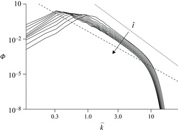


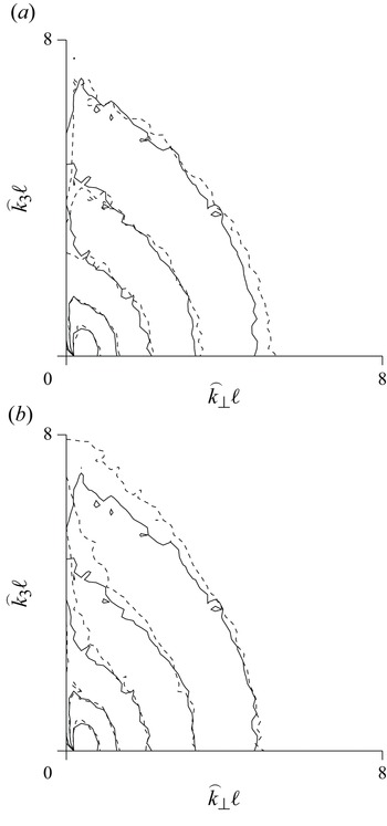


 Open access