


1. Introduction
Rayleigh–Bénard–Poiseuille (RBP) flows describe the motion of fluids confined between two extended parallel plates, heated from below and cooled from the top, with an imposed pressure gradient. This system combines the classical Rayleigh–Bénard convection (RBC) and plane Poiseuille flow (PPF), driven by buoyancy and shear forces, respectively. In the limiting cases, the laminar solution can transition to convection rolls (RBC), or shear-driven turbulence (PPF), depending on whether buoyancy or shear forces dominate. Transition to turbulence in the regime where both forces interact remains largely unexplored. For instance, do buoyancy forces promote the transition to shear-driven turbulence? How does shear influence the convection? Understanding the transition to turbulence in this regime can have implications for applications such as the fabrication of thin uniform films in the deposition of chemical vapours (Evans & Greif Reference Evans and Greif1991; Jensen, Einset & Fotiadis Reference Jensen, Einset and Fotiadis1991) and the cooling of electronic components (Kennedy & Zebib Reference Kennedy and Zebib1983; Ray & Srinivasan Reference Ray and Srinivasan1992).
1.1. Rayleigh–Bénard–Poiseuille (RBP) flows
The non-dimensionalised parameters that govern the RBP flow are the Rayleigh number, $Ra = 8\eta g h^3 \Delta T / \nu \kappa$
, Reynolds number,
$Ra = 8\eta g h^3 \Delta T / \nu \kappa$
, Reynolds number, $\textit{Re} = U_c h / \nu$
, Prandtl number,
$\textit{Re} = U_c h / \nu$
, Prandtl number, $\textit{Pr} = \nu / \kappa$
, and the aspect ratio of the flow domain,
$\textit{Pr} = \nu / \kappa$
, and the aspect ratio of the flow domain, $\varGamma = L/h$
, where
$\varGamma = L/h$
, where $\eta , g, \Delta T, \nu , \kappa , U_c, h, L$
are the thermal expansion coefficient, acceleration due to gravity, temperature difference between the bottom and top walls, kinematic viscosity, thermal diffusivity, laminar centreline velocity, domain half-depth, and length (or span), respectively. The spatial coordinate vector,
$\eta , g, \Delta T, \nu , \kappa , U_c, h, L$
are the thermal expansion coefficient, acceleration due to gravity, temperature difference between the bottom and top walls, kinematic viscosity, thermal diffusivity, laminar centreline velocity, domain half-depth, and length (or span), respectively. The spatial coordinate vector, $\boldsymbol{x} = (x,y,z)$
, is non-dimensionalised by
$\boldsymbol{x} = (x,y,z)$
, is non-dimensionalised by $h$
, where
$h$
, where $x$
,
$x$
, $y$
and
$y$
and $z$
refer to the streamwise, wall-normal and spanwise directions, respectively.
$z$
refer to the streamwise, wall-normal and spanwise directions, respectively.
Gage & Reid (Reference Gage and Reid1968) first investigated the primary instabilities of RBP flows, which can be determined by $\textit{Re}$
,
$\textit{Re}$
, $Ra$
,
$Ra$
, $\textit{Pr}$
and the perturbation wavenumbers in the
$\textit{Pr}$
and the perturbation wavenumbers in the $x$
and
$x$
and $z$
directions,
$z$
directions, $\alpha$
and
$\alpha$
and $\beta$
. For a given
$\beta$
. For a given $Ra$
and
$Ra$
and $\textit{Pr}$
, the neutral stability curves are limited by the development of Tollmien–Schlichting waves for
$\textit{Pr}$
, the neutral stability curves are limited by the development of Tollmien–Schlichting waves for $\textit{Re} \geqslant \textit{Re}_{\textit{TS}} = 5772.22$
(Orszag Reference Orszag1971) and convection rolls within
$\textit{Re} \geqslant \textit{Re}_{\textit{TS}} = 5772.22$
(Orszag Reference Orszag1971) and convection rolls within $0 \leqslant \textit{Re} \lt \textit{Re}_{\textit{TS}}$
. Convection rolls can be categorised based on their orientation to the mean flow, namely, longitudinal (
$0 \leqslant \textit{Re} \lt \textit{Re}_{\textit{TS}}$
. Convection rolls can be categorised based on their orientation to the mean flow, namely, longitudinal ( $\alpha = 0, \beta \neq 0$
), transverse (
$\alpha = 0, \beta \neq 0$
), transverse ( $\alpha \neq 0, \beta = 0$
) and oblique rolls (
$\alpha \neq 0, \beta = 0$
) and oblique rolls ( $\alpha \neq 0, \beta \neq 0$
). The eigenvalue problem of the linearised system for the onset of longitudinal rolls is identical to that of the linearised RBC system, with the critical Rayleigh number for the linear instability,
$\alpha \neq 0, \beta \neq 0$
). The eigenvalue problem of the linearised system for the onset of longitudinal rolls is identical to that of the linearised RBC system, with the critical Rayleigh number for the linear instability, $Ra_{\parallel } = Ra_{\textit{RB}} = 1708.8$
and the corresponding critical wavenumber,
$Ra_{\parallel } = Ra_{\textit{RB}} = 1708.8$
and the corresponding critical wavenumber, $\alpha _{\parallel } = \alpha _{\textit{RB}} = 3.13$
(Pellew & Southwell Reference Pellew and Southwell1940; Kelly Reference Kelly1994), independent of
$\alpha _{\parallel } = \alpha _{\textit{RB}} = 3.13$
(Pellew & Southwell Reference Pellew and Southwell1940; Kelly Reference Kelly1994), independent of $\textit{Re}$
and
$\textit{Re}$
and $\textit{Pr}$
(
$\textit{Pr}$
( $Ra_{\textit{RB}}$
and
$Ra_{\textit{RB}}$
and $\alpha _{\textit{RB}}$
are the critical Rayleigh number and wavenumber for the linear instability of the Rayleigh–Bénard convection). The critical Rayleigh number for the oblique and transverse rolls matches that of RBC at
$\alpha _{\textit{RB}}$
are the critical Rayleigh number and wavenumber for the linear instability of the Rayleigh–Bénard convection). The critical Rayleigh number for the oblique and transverse rolls matches that of RBC at $\textit{Re}=0$
due to horizontal isotropy, but increases as
$\textit{Re}=0$
due to horizontal isotropy, but increases as $\textit{Re}$
increases and is dependent on
$\textit{Re}$
increases and is dependent on $\textit{Pr}$
(Gage & Reid Reference Gage and Reid1968; Müller et al. Reference Müller, Lücke and Kamps1992; Nicolas, Mojtabi & Platten Reference Nicolas, Mojtabi and Platten1997). When the spatio-temporal development of instabilities is concerned, longitudinal rolls are always convectively unstable and transverse rolls can become absolutely unstable (Müller et al. Reference Müller, Lücke and Kamps1989; Müller et al. Reference Müller, Lücke and Kamps1992; Carrière & Monkewitz Reference Carrière and Monkewitz1999). Moreover, weakly nonlinear analysis of transverse and longitudinal rolls has been performed (Carrière & Monkewitz Reference Carrière and Monkewitz2001; Carrière et al. Reference Carrière, Monkewitz and Martinand2004), and the results have been verified experimentally (Grandjean & Monkewitz Reference Grandjean and Monkewitz2009). Non-modal stability analysis of subcritical RBP flows indicates that optimal transient growth,
$\textit{Pr}$
(Gage & Reid Reference Gage and Reid1968; Müller et al. Reference Müller, Lücke and Kamps1992; Nicolas, Mojtabi & Platten Reference Nicolas, Mojtabi and Platten1997). When the spatio-temporal development of instabilities is concerned, longitudinal rolls are always convectively unstable and transverse rolls can become absolutely unstable (Müller et al. Reference Müller, Lücke and Kamps1989; Müller et al. Reference Müller, Lücke and Kamps1992; Carrière & Monkewitz Reference Carrière and Monkewitz1999). Moreover, weakly nonlinear analysis of transverse and longitudinal rolls has been performed (Carrière & Monkewitz Reference Carrière and Monkewitz2001; Carrière et al. Reference Carrière, Monkewitz and Martinand2004), and the results have been verified experimentally (Grandjean & Monkewitz Reference Grandjean and Monkewitz2009). Non-modal stability analysis of subcritical RBP flows indicates that optimal transient growth, $G_{\textit{max}}$
, gradually increases with
$G_{\textit{max}}$
, gradually increases with $Ra$
. The wavenumber of the optimal initial condition,
$Ra$
. The wavenumber of the optimal initial condition, $\beta _{\textit{max}}$
, resembles that observed in shear flows (Reddy & Henningson Reference Reddy and Henningson1993) and gradually approaches the critical wavenumber of convection rolls,
$\beta _{\textit{max}}$
, resembles that observed in shear flows (Reddy & Henningson Reference Reddy and Henningson1993) and gradually approaches the critical wavenumber of convection rolls, $\alpha _{\parallel }$
, as
$\alpha _{\parallel }$
, as $Ra$
increases (Jerome, Chomaz & Huerre Reference Jerome, Chomaz and Huerre2012). For
$Ra$
increases (Jerome, Chomaz & Huerre Reference Jerome, Chomaz and Huerre2012). For $\textit{Re} \gt 0$
, longitudinal rolls appear as the dominant primary instability (Gage & Reid Reference Gage and Reid1968). Secondary stability analysis of the longitudinal rolls reveals a wavy instability near
$\textit{Re} \gt 0$
, longitudinal rolls appear as the dominant primary instability (Gage & Reid Reference Gage and Reid1968). Secondary stability analysis of the longitudinal rolls reveals a wavy instability near $\textit{Re} \sim 100$
(Clever & Busse Reference Clever and Busse1991), leading to wavy longitudinal rolls, which are convectively unstable (Pabiou, Mergui & Bénard Reference Pabiou, Mergui and Bénard2005; Nicolas, Zoueidi & Xin Reference Nicolas, Zoueidi and Xin2012). The influence of finite lateral extensions in RBP flows on the stability of longitudinal and transverse rolls (Kato & Fujimura Reference Kato and Fujimura2000; Nicolas, Luijkx & Platten Reference Nicolas, Luijkx and Platten2000), as well as wavy rolls (Xin, Nicolas & Quéré Reference Xin, Nicolas and Quéré2006; Nicolas et al. Reference Nicolas, Zoueidi and Xin2012), have been reported. In finite streamwise extensions of RBP flows, the onset of convection rolls and the heat flux variations due to entrance effects have been investigated (Mahaney et al. Reference Mahaney, Incropera and Ramadhyani1988; Lee & Hwang Reference Lee and Hwang1991; Nonino & Giudice Reference Nonino and Giudice1991). More recently, it has been shown that shear-driven turbulence can enhance heat fluxes in turbulent RBP flows (Scagliarini, Gylfason & Toschi Reference Scagliarini, Gylfason and Toschi2014; Pirozzoli et al. Reference Pirozzoli, Bernardini, Verzicco and Orlandi2017; Blass et al. Reference Blass, Zhu, Verzicco, Lohse and Stevens2020, Reference Blass, Tabak, Verzicco, Stevens and Lohse2021; Yerragolam et al. Reference Yerragolam, Howland, Stevens, Verzicco, Shishkina and Lohse2024). RBP flows with sinusoidal heating and walls, potentially leading to drag reductions, have been well studied (Hossain, Floryan & Floryan Reference Hossain, Floryan and Floryan2012; Hossain & Floryan Reference Hossain and Floryan2015, Reference Hossain and Floryan2016, Reference Hossain and Floryan2020). Finally, RBP flows in rotating tilted domains have also been reported (Perez-Espejel & Avila Reference Perez-Espejel and Avila2019). For an in-depth discussion of RBP flows, see the reviews by Kelly (Reference Kelly1994) and Nicolas (Reference Nicolas2002).
$\textit{Re} \sim 100$
(Clever & Busse Reference Clever and Busse1991), leading to wavy longitudinal rolls, which are convectively unstable (Pabiou, Mergui & Bénard Reference Pabiou, Mergui and Bénard2005; Nicolas, Zoueidi & Xin Reference Nicolas, Zoueidi and Xin2012). The influence of finite lateral extensions in RBP flows on the stability of longitudinal and transverse rolls (Kato & Fujimura Reference Kato and Fujimura2000; Nicolas, Luijkx & Platten Reference Nicolas, Luijkx and Platten2000), as well as wavy rolls (Xin, Nicolas & Quéré Reference Xin, Nicolas and Quéré2006; Nicolas et al. Reference Nicolas, Zoueidi and Xin2012), have been reported. In finite streamwise extensions of RBP flows, the onset of convection rolls and the heat flux variations due to entrance effects have been investigated (Mahaney et al. Reference Mahaney, Incropera and Ramadhyani1988; Lee & Hwang Reference Lee and Hwang1991; Nonino & Giudice Reference Nonino and Giudice1991). More recently, it has been shown that shear-driven turbulence can enhance heat fluxes in turbulent RBP flows (Scagliarini, Gylfason & Toschi Reference Scagliarini, Gylfason and Toschi2014; Pirozzoli et al. Reference Pirozzoli, Bernardini, Verzicco and Orlandi2017; Blass et al. Reference Blass, Zhu, Verzicco, Lohse and Stevens2020, Reference Blass, Tabak, Verzicco, Stevens and Lohse2021; Yerragolam et al. Reference Yerragolam, Howland, Stevens, Verzicco, Shishkina and Lohse2024). RBP flows with sinusoidal heating and walls, potentially leading to drag reductions, have been well studied (Hossain, Floryan & Floryan Reference Hossain, Floryan and Floryan2012; Hossain & Floryan Reference Hossain and Floryan2015, Reference Hossain and Floryan2016, Reference Hossain and Floryan2020). Finally, RBP flows in rotating tilted domains have also been reported (Perez-Espejel & Avila Reference Perez-Espejel and Avila2019). For an in-depth discussion of RBP flows, see the reviews by Kelly (Reference Kelly1994) and Nicolas (Reference Nicolas2002).
1.2. Rayleigh–Bénard convection (RBC)
In the limiting case of $\textit{Re} = 0$
, the RBP problem reduces to the classical Rayleigh–Bénard convection (RBC). We provide an overview of the key developments of RBC as a foundation for studying RBP flows at
$\textit{Re} = 0$
, the RBP problem reduces to the classical Rayleigh–Bénard convection (RBC). We provide an overview of the key developments of RBC as a foundation for studying RBP flows at $\textit{Re} = 0$
. Beyond the onset,
$\textit{Re} = 0$
. Beyond the onset, $Ra \gt Ra_{\textit{RB}}$
, the secondary stability characteristics of ideal straight rolls (ISRs), which are infinitely parallel convection rolls, are described by the Busse balloon (Busse Reference Busse1978). This balloon defines the stability boundaries of ISRs based on their wavenumber,
$Ra \gt Ra_{\textit{RB}}$
, the secondary stability characteristics of ideal straight rolls (ISRs), which are infinitely parallel convection rolls, are described by the Busse balloon (Busse Reference Busse1978). This balloon defines the stability boundaries of ISRs based on their wavenumber, $Ra$
and
$Ra$
and $\textit{Pr}$
. For
$\textit{Pr}$
. For $\textit{Pr} = 1$
and
$\textit{Pr} = 1$
and $ Ra \gt Ra_{\textit{RB}}$
, the secondary instabilities primarily modify the ISR wavenumber, so that it remains within the boundaries of the Busse balloon. These include the cross-roll, Eckhaus and skewed-varicose instabilities (Busse Reference Busse1978; Busse & Clever Reference Busse and Clever1979; Bodenschatz, Pesch & Ahlers Reference Bodenschatz, Pesch and Ahlers2000). An oscillatory secondary instability emerges at
$ Ra \gt Ra_{\textit{RB}}$
, the secondary instabilities primarily modify the ISR wavenumber, so that it remains within the boundaries of the Busse balloon. These include the cross-roll, Eckhaus and skewed-varicose instabilities (Busse Reference Busse1978; Busse & Clever Reference Busse and Clever1979; Bodenschatz, Pesch & Ahlers Reference Bodenschatz, Pesch and Ahlers2000). An oscillatory secondary instability emerges at $Ra \gtrsim 5000$
, where a stationary ISR transitions into a time-dependent tertiary state, known as oscillatory ISRs (Clever & Busse Reference Clever and Busse1974; Bodenschatz et al. Reference Bodenschatz, Pesch and Ahlers2000), and these instabilities have been reported in experiments (Willis & Deardorff Reference Willis and Deardorff1970; Steinberg, Ahlers & Cannell Reference Steinberg, Ahlers and Cannell1985; Croquette Reference Croquette1989; Bodenschatz et al. Reference Bodenschatz, Pesch and Ahlers2000). Notably, ISRs appear to be the exception rather than the norm as multiple convection patterns have been reported in the form of squares, targets and oscillatory convection patterns, resulting in many multiple stable states in the same
$Ra \gtrsim 5000$
, where a stationary ISR transitions into a time-dependent tertiary state, known as oscillatory ISRs (Clever & Busse Reference Clever and Busse1974; Bodenschatz et al. Reference Bodenschatz, Pesch and Ahlers2000), and these instabilities have been reported in experiments (Willis & Deardorff Reference Willis and Deardorff1970; Steinberg, Ahlers & Cannell Reference Steinberg, Ahlers and Cannell1985; Croquette Reference Croquette1989; Bodenschatz et al. Reference Bodenschatz, Pesch and Ahlers2000). Notably, ISRs appear to be the exception rather than the norm as multiple convection patterns have been reported in the form of squares, targets and oscillatory convection patterns, resulting in many multiple stable states in the same $Ra$
parameter space where ISRs are expected (Le Gal, Pocheau & Croquette Reference Le Gal, Pocheau and Croquette1985; Croquette Reference Croquette1989; Plapp & Bodenschatz Reference Plapp and Bodenschatz1996; Hof, Lucas & Mullin Reference Hof, Lucas and Mullin1999; Rüdiger & Feudel Reference Rüdiger and Feudel2000; Borońska & Tuckerman Reference Borońska and Tuckerman2010a
,Reference Borońska and Tuckerman
b
; Chan et al. Reference Chan, Hossain, Sherwin and Hwang2026). For large aspect ratios,
$Ra$
parameter space where ISRs are expected (Le Gal, Pocheau & Croquette Reference Le Gal, Pocheau and Croquette1985; Croquette Reference Croquette1989; Plapp & Bodenschatz Reference Plapp and Bodenschatz1996; Hof, Lucas & Mullin Reference Hof, Lucas and Mullin1999; Rüdiger & Feudel Reference Rüdiger and Feudel2000; Borońska & Tuckerman Reference Borońska and Tuckerman2010a
,Reference Borońska and Tuckerman
b
; Chan et al. Reference Chan, Hossain, Sherwin and Hwang2026). For large aspect ratios, $\varGamma \gtrsim 80$
, convection rolls can exhibit spatio-temporal chaotic behaviour, known as spiral defect chaos (SDC) within the same range of
$\varGamma \gtrsim 80$
, convection rolls can exhibit spatio-temporal chaotic behaviour, known as spiral defect chaos (SDC) within the same range of $Ra$
(Morris et al. Reference Morris, Bodenschatz, Cannell and Ahlers1993; Decker, Pesch & Weber Reference Decker, Pesch and Weber1994; Hu, Ecke & Ahlers Reference Hu, Ecke and Ahlers1995; Morris et al. Reference Morris, Bodenschatz, Cannell and Ahlers1996; Cakmur et al. Reference Cakmur, Egolf, Plapp and Bodenschatz1997; Ahlers Reference Ahlers1998; Egolf, Melnikov & Bodenschatz Reference Egolf, Melnikov and Bodenschatz1998; Chiam et al. Reference Chiam, Paul, Cross and Greenside2003; Vitral et al. Reference Vitral, Mukherjee, Leo, Viñals, Paul and Huang2020). It is now established that both SDC and ISR can coexist at the same
$Ra$
(Morris et al. Reference Morris, Bodenschatz, Cannell and Ahlers1993; Decker, Pesch & Weber Reference Decker, Pesch and Weber1994; Hu, Ecke & Ahlers Reference Hu, Ecke and Ahlers1995; Morris et al. Reference Morris, Bodenschatz, Cannell and Ahlers1996; Cakmur et al. Reference Cakmur, Egolf, Plapp and Bodenschatz1997; Ahlers Reference Ahlers1998; Egolf, Melnikov & Bodenschatz Reference Egolf, Melnikov and Bodenschatz1998; Chiam et al. Reference Chiam, Paul, Cross and Greenside2003; Vitral et al. Reference Vitral, Mukherjee, Leo, Viñals, Paul and Huang2020). It is now established that both SDC and ISR can coexist at the same $Ra$
, forming a bistable system confirmed experimentally (Cakmur et al. Reference Cakmur, Egolf, Plapp and Bodenschatz1997).
$Ra$
, forming a bistable system confirmed experimentally (Cakmur et al. Reference Cakmur, Egolf, Plapp and Bodenschatz1997).
1.3. Plane Poiseuille flows (PPF)
The other limiting case at $Ra = 0$
corresponds to the PPF and its relevance to RBP flows is discussed here. Turbulence in PPF is known to be subcritical, occurring well below the threshold of linear instability,
$Ra = 0$
corresponds to the PPF and its relevance to RBP flows is discussed here. Turbulence in PPF is known to be subcritical, occurring well below the threshold of linear instability, $\textit{Re} \lt \textit{Re}_{\textit{TS}}$
(Davies & White Reference Davies and White1928; Patel & Head Reference Patel and Head1969). The initial evolution of a small disturbance given in the flow is influenced by the non-normality of the linearised Navier–Stokes equations, allowing it to undergo significant transient growth (Reddy & Henningson Reference Reddy and Henningson1993; Schmid Reference Schmid2007). The optimal initial condition involves streamwise vortices which amplify streaks, related to the lift-up effect (Ellingsen & Palm Reference Ellingsen and Palm1975; Butler & Farrell Reference Butler and Farrell1992). While modal and non-modal methods describe the time evolution of small perturbations about the laminar state, turbulence in wall-bounded shear flows may emerge well before the onset of the linear instability (i.e. Tollmien–Schlichting mode). This indicates the existence of non-trivial nonlinear solutions, motivating a nonlinear dynamical systems approach. A key development in this framework is the identification of pairs of unstable invariant states that emerge through saddle-node bifurcations, forming the so-called upper and lower branches. These branches are disconnected from the laminar solution, distinguished by their proximity to the laminar solution (Waleffe Reference Waleffe2001, Reference Waleffe2003; Nagata & Deguchi Reference Nagata and Deguchi2013; Gibson & Brand Reference Gibson and Brand2014; Park & Graham Reference Park and Graham2015; Wall & Nagata Reference Wall and Nagata2016). A rich family of invariant states, such as equilibria, travelling waves, periodic orbits, relative periodic orbits, exists around the upper and lower branch solutions. Together, they have been envisioned to form a building block description of turbulence particularly in plane Couette flows (Nagata Reference Nagata1990, Reference Nagata1997; Clever & Busse Reference Clever and Busse1997; Kawahara & Kida Reference Kawahara and Kida2001; Viswanath Reference Viswanath2007; Gibson, Halcrow & Cvitanović Reference Gibson, Halcrow and Cvitanović2009; Cvitanović & Gibson Reference Cvitanović and Gibson2010), describing the self-sustaining process (Hamilton, Kim & Waleffe Reference Hamilton, Kim and Waleffe1995). In some cases, notably pipe flows, a collection of lower branch solutions was found to lie on the basin boundary (i.e. the edge) between the laminar and turbulent attractors (Kerswell & Tutty Reference Kerswell and Tutty2007; Pringle & Kerswell Reference Pringle and Kerswell2007; Duguet, Willis & Kerswell Reference Duguet, Willis and Kerswell2008), although both upper and lower branches have been found to lie on the edge in PPF (Wall & Nagata Reference Wall and Nagata2016). As
$\textit{Re} \lt \textit{Re}_{\textit{TS}}$
(Davies & White Reference Davies and White1928; Patel & Head Reference Patel and Head1969). The initial evolution of a small disturbance given in the flow is influenced by the non-normality of the linearised Navier–Stokes equations, allowing it to undergo significant transient growth (Reddy & Henningson Reference Reddy and Henningson1993; Schmid Reference Schmid2007). The optimal initial condition involves streamwise vortices which amplify streaks, related to the lift-up effect (Ellingsen & Palm Reference Ellingsen and Palm1975; Butler & Farrell Reference Butler and Farrell1992). While modal and non-modal methods describe the time evolution of small perturbations about the laminar state, turbulence in wall-bounded shear flows may emerge well before the onset of the linear instability (i.e. Tollmien–Schlichting mode). This indicates the existence of non-trivial nonlinear solutions, motivating a nonlinear dynamical systems approach. A key development in this framework is the identification of pairs of unstable invariant states that emerge through saddle-node bifurcations, forming the so-called upper and lower branches. These branches are disconnected from the laminar solution, distinguished by their proximity to the laminar solution (Waleffe Reference Waleffe2001, Reference Waleffe2003; Nagata & Deguchi Reference Nagata and Deguchi2013; Gibson & Brand Reference Gibson and Brand2014; Park & Graham Reference Park and Graham2015; Wall & Nagata Reference Wall and Nagata2016). A rich family of invariant states, such as equilibria, travelling waves, periodic orbits, relative periodic orbits, exists around the upper and lower branch solutions. Together, they have been envisioned to form a building block description of turbulence particularly in plane Couette flows (Nagata Reference Nagata1990, Reference Nagata1997; Clever & Busse Reference Clever and Busse1997; Kawahara & Kida Reference Kawahara and Kida2001; Viswanath Reference Viswanath2007; Gibson, Halcrow & Cvitanović Reference Gibson, Halcrow and Cvitanović2009; Cvitanović & Gibson Reference Cvitanović and Gibson2010), describing the self-sustaining process (Hamilton, Kim & Waleffe Reference Hamilton, Kim and Waleffe1995). In some cases, notably pipe flows, a collection of lower branch solutions was found to lie on the basin boundary (i.e. the edge) between the laminar and turbulent attractors (Kerswell & Tutty Reference Kerswell and Tutty2007; Pringle & Kerswell Reference Pringle and Kerswell2007; Duguet, Willis & Kerswell Reference Duguet, Willis and Kerswell2008), although both upper and lower branches have been found to lie on the edge in PPF (Wall & Nagata Reference Wall and Nagata2016). As $\textit{Re}$
increases beyond the saddle-node bifurcation, the upper branch can undergo a sequence of bifurcations, ultimately reconnecting with the lower branch. This leads to an exterior (boundary) crisis bifurcation, where the chaotic attractor becomes leaky, transforming into a chaotic saddle that permits an avenue towards the laminar state (Kreilos & Eckhardt Reference Kreilos and Eckhardt2012; Zammert & Eckhardt Reference Zammert and Eckhardt2015). The emergence of a chaotic saddle is consistent with experimental and numerical evidence of transient turbulence that eventually relaminarises (Bottin et al. Reference Bottin, Daviaud, Manneville and Dauchot1998; Hof et al. Reference Hof, Westerweel, Schneider and Eckhardt2006; Zammert & Eckhardt Reference Zammert and Eckhardt2015; Tuckerman, Chantry & Barkley Reference Tuckerman, Chantry and Barkley2020; Paranjape et al. Reference Paranjape, Yalnız, Duguet, Budanur and Hof2023). For a comprehensive review of the dynamical systems approach to shear-driven turbulence, the reader is referred to Kawahara et al. (Reference Kawahara, Uhlmann and van Veen2012) and Graham & Floryan (Reference Graham and Floryan2021).
$\textit{Re}$
increases beyond the saddle-node bifurcation, the upper branch can undergo a sequence of bifurcations, ultimately reconnecting with the lower branch. This leads to an exterior (boundary) crisis bifurcation, where the chaotic attractor becomes leaky, transforming into a chaotic saddle that permits an avenue towards the laminar state (Kreilos & Eckhardt Reference Kreilos and Eckhardt2012; Zammert & Eckhardt Reference Zammert and Eckhardt2015). The emergence of a chaotic saddle is consistent with experimental and numerical evidence of transient turbulence that eventually relaminarises (Bottin et al. Reference Bottin, Daviaud, Manneville and Dauchot1998; Hof et al. Reference Hof, Westerweel, Schneider and Eckhardt2006; Zammert & Eckhardt Reference Zammert and Eckhardt2015; Tuckerman, Chantry & Barkley Reference Tuckerman, Chantry and Barkley2020; Paranjape et al. Reference Paranjape, Yalnız, Duguet, Budanur and Hof2023). For a comprehensive review of the dynamical systems approach to shear-driven turbulence, the reader is referred to Kawahara et al. (Reference Kawahara, Uhlmann and van Veen2012) and Graham & Floryan (Reference Graham and Floryan2021).
In large spatial domains near the onset, turbulence in PPF appears as spatio-temporal intermittent turbulent–laminar bands, where turbulent and laminar regions can co-exist (Tsukahara et al. Reference Tsukahara, Iwamoto, Kawamura and Takeda2014a
,
Reference Tsukahara, Seki, Kawamura and Tochiob
; Tuckerman et al. Reference Tuckerman, Kreilos, Schrobsdorff, Schneider and Gibson2014; Shimizu & Manneville Reference Shimizu and Manneville2019; Gomé et al. Reference Gomé, Tuckerman and Barkley2020; Tuckerman et al. Reference Tuckerman, Chantry and Barkley2020; Paranjape et al. Reference Paranjape, Yalnız, Duguet, Budanur and Hof2023). Similar patterns have been observed in plane Couette flow (Prigent et al. Reference Prigent, Grégoire, Chaté and Dauchot2003; Barkley & Tuckerman Reference Barkley and Tuckerman2005; Duguet, Schlatter & Henningson Reference Duguet, Schlatter and Henningson2010; Tuckerman & Barkley Reference Tuckerman and Barkley2011; Reetz, Kreilos & Schneider Reference Reetz, Kreilos and Schneider2019) and pipe flows (Avila et al. Reference Avila, Moxey, de Lozar, Avila, Barkley and Hof2011; Song et al. Reference Song, Barkley, Hof and Avila2017; Avila, Barkley & Hof Reference Avila, Barkley and Hof2023). Depending on the magnitude of $\textit{Re}$
, these turbulent–laminar bands may split or decay spontaneously (Tuckerman et al. Reference Tuckerman, Kreilos, Schrobsdorff, Schneider and Gibson2014; Gomé et al. Reference Gomé, Tuckerman and Barkley2020), similar to the puff splitting and decay process in transitional pipe flows (Avila et al. Reference Avila, Barkley and Hof2023). The mean splitting and decay lifetime follow a Poisson process, with a superexponential dependence on
$\textit{Re}$
, these turbulent–laminar bands may split or decay spontaneously (Tuckerman et al. Reference Tuckerman, Kreilos, Schrobsdorff, Schneider and Gibson2014; Gomé et al. Reference Gomé, Tuckerman and Barkley2020), similar to the puff splitting and decay process in transitional pipe flows (Avila et al. Reference Avila, Barkley and Hof2023). The mean splitting and decay lifetime follow a Poisson process, with a superexponential dependence on $\textit{Re}$
. The decay lifetime increases while the splitting lifetime decreases with increasing
$\textit{Re}$
. The decay lifetime increases while the splitting lifetime decreases with increasing $\textit{Re}$
. The cross-over point where both the mean splitting and decay lifetime intersect at
$\textit{Re}$
. The cross-over point where both the mean splitting and decay lifetime intersect at $\textit{Re}_{\textit{cross}} \approx 965$
, marking a statistical critical Reynolds number for the onset of turbulent–laminar bands (Gomé et al. Reference Gomé, Tuckerman and Barkley2020). More recently, the invariant solutions corresponding to turbulent–laminar bands in large spanwise domains have been identified (Reetz et al. Reference Reetz, Kreilos and Schneider2019; Paranjape, Duguet & Hof Reference Paranjape, Duguet and Hof2020, Reference Paranjape, Yalnız, Duguet, Budanur and Hof2023). These solutions appear to be connected to a periodic orbit originating from a travelling-wave lower branch of PPF (Paranjape et al. Reference Paranjape, Yalnız, Duguet, Budanur and Hof2023). For a detailed review of turbulent–laminar bands in wall-bounded shear flows, the reader is referred to Tuckerman et al. (Reference Tuckerman, Chantry and Barkley2020).
$\textit{Re}_{\textit{cross}} \approx 965$
, marking a statistical critical Reynolds number for the onset of turbulent–laminar bands (Gomé et al. Reference Gomé, Tuckerman and Barkley2020). More recently, the invariant solutions corresponding to turbulent–laminar bands in large spanwise domains have been identified (Reetz et al. Reference Reetz, Kreilos and Schneider2019; Paranjape, Duguet & Hof Reference Paranjape, Duguet and Hof2020, Reference Paranjape, Yalnız, Duguet, Budanur and Hof2023). These solutions appear to be connected to a periodic orbit originating from a travelling-wave lower branch of PPF (Paranjape et al. Reference Paranjape, Yalnız, Duguet, Budanur and Hof2023). For a detailed review of turbulent–laminar bands in wall-bounded shear flows, the reader is referred to Tuckerman et al. (Reference Tuckerman, Chantry and Barkley2020).
1.4. Objectives and organisation
While the linear stability characteristics of laminar RBP flows have been well studied (see § 1.1), the transition to shear-driven turbulence and the related nonlinear dynamics remain largely unexplored. As the first step towards understanding the transition in RBP flows, the main objective of this work is to perform exploratory direct numerical simulation (DNS) studies of transitional RBP flows while investigating the impact of $\textit{Re}$
on the bistability between SDC and ISRs in RBC as well as the influence of
$\textit{Re}$
on the bistability between SDC and ISRs in RBC as well as the influence of $Ra$
on turbulent–laminar bands in PPF. For this purpose, we consider a relatively wide range of parameter space given by
$Ra$
on turbulent–laminar bands in PPF. For this purpose, we consider a relatively wide range of parameter space given by $Ra \in [0, 10000]$
and
$Ra \in [0, 10000]$
and $\textit{Re} \in [0, 2000]$
at
$\textit{Re} \in [0, 2000]$
at $\textit{Pr} = 1$
in both large and small domains (
$\textit{Pr} = 1$
in both large and small domains ( $\varGamma = 16\pi$
,
$\varGamma = 16\pi$
, $2\pi$
, in particular). Given that this study is largely exploratory, we will focus on identifying different flow regimes and providing key insights into their dynamical processes. We do not intend to perform an extensive bifurcation analysis that involves the computation and analysis of the invariant solutions, which could be computationally very costly, especially in a large domain.
$2\pi$
, in particular). Given that this study is largely exploratory, we will focus on identifying different flow regimes and providing key insights into their dynamical processes. We do not intend to perform an extensive bifurcation analysis that involves the computation and analysis of the invariant solutions, which could be computationally very costly, especially in a large domain.
The paper is organised as follows. In § 2, we describe problem formulation, governing equations, numerical methods and set-up. In § 3, we present the $Ra$
–
$Ra$
– $\textit{Re}$
phase space, identifying five distinct regimes and their coarse-grained transition boundaries. We also show a new ‘intermittent roll’ regime and discuss the coexistence of longitudinal rolls with turbulent–laminar bands, highlighting the central role of longitudinal rolls in transitional RBP flows in large domains,
$\textit{Re}$
phase space, identifying five distinct regimes and their coarse-grained transition boundaries. We also show a new ‘intermittent roll’ regime and discuss the coexistence of longitudinal rolls with turbulent–laminar bands, highlighting the central role of longitudinal rolls in transitional RBP flows in large domains, $\varGamma = 16\pi$
. In § 4, we perform a numerical experiment, in which simulations are performed along the unstable manifolds of longitudinal rolls in a small domain,
$\varGamma = 16\pi$
. In § 4, we perform a numerical experiment, in which simulations are performed along the unstable manifolds of longitudinal rolls in a small domain, $\varGamma = 2\pi$
. We will see that this reveals some dynamical connections among shear-driven turbulence, longitudinal rolls and the laminar state, and subsequently discuss their relevance to large domains,
$\varGamma = 2\pi$
. We will see that this reveals some dynamical connections among shear-driven turbulence, longitudinal rolls and the laminar state, and subsequently discuss their relevance to large domains, $\varGamma = 16\pi$
. Finally, we conclude in § 5 and provide some perspectives for future work.
$\varGamma = 16\pi$
. Finally, we conclude in § 5 and provide some perspectives for future work.
2. Problem formulation
2.1. Governing equations
We consider a layer of fluid sandwiched between two extended parallel plates, separated by depth $2h$
, with a uniform upper and lower plate temperature
$2h$
, with a uniform upper and lower plate temperature $T_U$
and
$T_U$
and $T_L$
. The horizontal size of the domain of interest is set with equal length and span,
$T_L$
. The horizontal size of the domain of interest is set with equal length and span, $L = L_x = L_z$
. The fluid is unstably stratified such that
$L = L_x = L_z$
. The fluid is unstably stratified such that $\Delta T = T_L - T_U \gt 0$
. The fluid has a density of
$\Delta T = T_L - T_U \gt 0$
. The fluid has a density of $\rho$
, kinetic viscosity,
$\rho$
, kinetic viscosity, $\nu$
, and thermal diffusivity,
$\nu$
, and thermal diffusivity, $\kappa$
. The non-dimensionalised governing equations, composed of the Navier–Stokes equations with Boussinesq approximation, the energy equation and the divergence free constrain, are given by
$\kappa$
. The non-dimensionalised governing equations, composed of the Navier–Stokes equations with Boussinesq approximation, the energy equation and the divergence free constrain, are given by
 \begin{equation} \frac {\partial \boldsymbol{u}}{\partial t} + (\boldsymbol{u}\boldsymbol{\cdot }\boldsymbol{\nabla })\boldsymbol{u} = -\boldsymbol{\nabla }\!p + \frac {1}{\textit{Re}}{\nabla} ^2 \boldsymbol{u} + \frac {Ra}{8\textit{PrRe}^2}\theta \boldsymbol{{j}}, \end{equation}
 \begin{equation} \frac {\partial \theta }{\partial t} + (\boldsymbol{u} \boldsymbol{\cdot }\boldsymbol{\nabla })\theta = \frac {1}{\textit{RePr}}{\nabla} ^2 \theta , \end{equation}
 \begin{equation} \boldsymbol{\nabla }\boldsymbol{\cdot }\boldsymbol{u} = 0, \end{equation}
with the following boundary conditions at the wall:
 \begin{equation} \boldsymbol{u}|_{y=\pm 1} = 0, \quad \theta |_{y = -1} = 1, \quad \theta |_{y=1} = 0, \end{equation}
and periodic boundary conditions in the planar $x$
and
$x$
and $z$
directions. The unit vector
$z$
directions. The unit vector $\boldsymbol{j}$
is in the
$\boldsymbol{j}$
is in the $y$
direction. The temporal coordinate
$y$
direction. The temporal coordinate $t$
denotes the time non-dimensionalised by the advective time scale,
$t$
denotes the time non-dimensionalised by the advective time scale, $U_c/h$
. Here,
$U_c/h$
. Here, $\boldsymbol{u}(\boldsymbol{x},t)$
is the velocity vector non-dimensionalised by the laminar centreline velocity,
$\boldsymbol{u}(\boldsymbol{x},t)$
is the velocity vector non-dimensionalised by the laminar centreline velocity, $U_c$
(i.e.
$U_c$
(i.e. $U_{\textit{lam}}(y)= U_c(1-y^2)$
),
$U_{\textit{lam}}(y)= U_c(1-y^2)$
), $p$
the pressure scaled by the dynamic pressure scale,
$p$
the pressure scaled by the dynamic pressure scale, $\rho U_c^2$
, and
$\rho U_c^2$
, and $\theta (\equiv (T-T_U)/\Delta T)$
the non-dimensionalised temperature with
$\theta (\equiv (T-T_U)/\Delta T)$
the non-dimensionalised temperature with $T$
being the absolute temperature. We note that the rescaled term
$T$
being the absolute temperature. We note that the rescaled term $Ra/8$
in the momentum forcing terms is equivalent to the Rayleigh number scaled based on the half-depth
$Ra/8$
in the momentum forcing terms is equivalent to the Rayleigh number scaled based on the half-depth $h$
, since
$h$
, since $Ra$
is scaled based on depth,
$Ra$
is scaled based on depth, $2h$
, as in classical RBC. The Rayleigh number
$2h$
, as in classical RBC. The Rayleigh number $Ra$
, Reynolds number
$Ra$
, Reynolds number $\textit{Re}$
and Prandtl number
$\textit{Re}$
and Prandtl number $\textit{Pr}$
are defined in § 1. We set
$\textit{Pr}$
are defined in § 1. We set $\textit{Pr} = 1$
in this study. For the Rayleigh–Bénard convection problem, we note that (2.1) becomes singular at
$\textit{Pr} = 1$
in this study. For the Rayleigh–Bénard convection problem, we note that (2.1) becomes singular at $\textit{Re} = 0$
. In such cases, we solve the non-dimensionalised incompressible Navier–Stokes equations based on thermal length, velocity and temporal scales shown in Appendix A.
$\textit{Re} = 0$
. In such cases, we solve the non-dimensionalised incompressible Navier–Stokes equations based on thermal length, velocity and temporal scales shown in Appendix A.
2.2. Numerical methods
The governing equations are solved numerically using an open-source spectral/hp-element package, Nektar++ (Cantwell et al. Reference Cantwell2015; Moxey et al. Reference Moxey2020). The computational mesh consists of two-dimensional (2-D) quadrilateral elements in the $y{-}z$
plane generated using Gmsh (Geuzaine & Remacle Reference Geuzaine and Remacle2009) and then imported into Nektar++ using Nekmesh (Green et al. Reference Green, Kirilov, Turner, Marcon, Eichstädt, Laughton, Cantwell, Sherwin, Peiró and Moxey2024). We discretise the spatial domain based on the quasi-three-dimensional (quasi-3-D) approach, employing spectral/hp elements in the
$y{-}z$
plane generated using Gmsh (Geuzaine & Remacle Reference Geuzaine and Remacle2009) and then imported into Nektar++ using Nekmesh (Green et al. Reference Green, Kirilov, Turner, Marcon, Eichstädt, Laughton, Cantwell, Sherwin, Peiró and Moxey2024). We discretise the spatial domain based on the quasi-three-dimensional (quasi-3-D) approach, employing spectral/hp elements in the $y{-}z$
plane and Fourier expansions in the streamwise direction
$y{-}z$
plane and Fourier expansions in the streamwise direction $x$
(Karniadakis Reference Karniadakis1989). The discretised equations are solved using a velocity correction scheme, based on a second-order stiffly splitting scheme, where the nonlinear advection and forcing terms are treated explicitly, while the pressure and diffusion terms are treated implicitly (Karniadakis, Israeli & Orszag Reference Karniadakis, Israeli and Orszag1991; Guermond & Shen Reference Guermond and Shen2003). The
$x$
(Karniadakis Reference Karniadakis1989). The discretised equations are solved using a velocity correction scheme, based on a second-order stiffly splitting scheme, where the nonlinear advection and forcing terms are treated explicitly, while the pressure and diffusion terms are treated implicitly (Karniadakis, Israeli & Orszag Reference Karniadakis, Israeli and Orszag1991; Guermond & Shen Reference Guermond and Shen2003). The $3/2$
and polynomial dealiasing rule for the Fourier expansions and spectral/hp elements are applied during the evaluation of the nonlinear advection terms. We refer to the solution obtained at the end of the velocity correction scheme as the homogeneous velocity
$3/2$
and polynomial dealiasing rule for the Fourier expansions and spectral/hp elements are applied during the evaluation of the nonlinear advection terms. We refer to the solution obtained at the end of the velocity correction scheme as the homogeneous velocity $\boldsymbol{u}_h$
. To sustain the flow for
$\boldsymbol{u}_h$
. To sustain the flow for $\textit{Re}\gt 0$
, we use a Green’s function approach (Chu et al. Reference Chu, Henderson and Karniadakis1992) to impose a constant flow rate,
$\textit{Re}\gt 0$
, we use a Green’s function approach (Chu et al. Reference Chu, Henderson and Karniadakis1992) to impose a constant flow rate,
 \begin{equation} U_b = Q(\boldsymbol{u})=\frac {1}{2 L_z h}\int _{ y,z} \boldsymbol{u}(0,y,z) \; \mathrm{d}y\,\mathrm{d}z, \end{equation}
where $U_b$
and
$U_b$
and $Q(\boldsymbol{\cdot })$
refer to the desired flow rate and flow rate operator. A correction velocity,
$Q(\boldsymbol{\cdot })$
refer to the desired flow rate and flow rate operator. A correction velocity, $\boldsymbol{u}_{\textit{corr}}$
, is obtained by solving the linear Stokes equations with unit forcing once and is stored for reuse. At the end of every time step, the final velocity field,
$\boldsymbol{u}_{\textit{corr}}$
, is obtained by solving the linear Stokes equations with unit forcing once and is stored for reuse. At the end of every time step, the final velocity field, $\boldsymbol{u}$
, is then updated by adding this correction velocity to the homogeneous velocity obtained from the velocity correction scheme,
$\boldsymbol{u}$
, is then updated by adding this correction velocity to the homogeneous velocity obtained from the velocity correction scheme,
 \begin{equation} \boldsymbol{u} = \boldsymbol{u}_h + \gamma \boldsymbol{u}_{\textit{corr}}, \end{equation}
where $\gamma$
, defined as
$\gamma$
, defined as
 \begin{equation} \gamma = \frac { U_b - Q(\boldsymbol{u}_h)}{Q(\boldsymbol{u}_{\textit{corr}})}, \end{equation}
is adjusted to satisfy the desired flow rate, $U_b$
. The flow rate,
$U_b$
. The flow rate, $U_b$
, is related to the laminar centreline velocity
$U_b$
, is related to the laminar centreline velocity $U_c = 3/2 U_b$
, which defines the Reynolds number,
$U_c = 3/2 U_b$
, which defines the Reynolds number, $\textit{Re} = U_c h / \nu$
. For more details on the numerical method, the reader is referred to Hossain, Cantwell & Sherwin (Reference Hossain, Cantwell and Sherwin2021).
$\textit{Re} = U_c h / \nu$
. For more details on the numerical method, the reader is referred to Hossain, Cantwell & Sherwin (Reference Hossain, Cantwell and Sherwin2021).
2.3. Parametric study in the $Ra$
–
$\textit{Re}$
space
$Ra$
–
$\textit{Re}$
space


We consider fifty-two numerical simulations at $\textit{Re} = 0, 0.1, 1, 10, 100, 500, 750, 1000,{} 1050$
,
$\textit{Re} = 0, 0.1, 1, 10, 100, 500, 750, 1000,{} 1050$
, $2000$
and
$2000$
and $Ra = 0, 2000, 3000, 5000, 8000, 10000$
at
$Ra = 0, 2000, 3000, 5000, 8000, 10000$
at $\textit{Pr} = 1$
with a large aspect ratio of
$\textit{Pr} = 1$
with a large aspect ratio of $\varGamma = 16\pi$
. The initial conditions of all cases are sampled from a statistically stationary solution. Laminar solutions are obtained for
$\varGamma = 16\pi$
. The initial conditions of all cases are sampled from a statistically stationary solution. Laminar solutions are obtained for $Ra = 0$
,
$Ra = 0$
, $\textit{Re} \leqslant 1000$
, with the given set of parameters and are omitted from the analysis. For all of the cases considered here, we maintain the same spatial resolution of
$\textit{Re} \leqslant 1000$
, with the given set of parameters and are omitted from the analysis. For all of the cases considered here, we maintain the same spatial resolution of $(\Delta x, \Delta y|_{y=\pm 1}, \Delta z) = (0.25\pi , 0.0549, 0.1\pi )$
with polynomial order
$(\Delta x, \Delta y|_{y=\pm 1}, \Delta z) = (0.25\pi , 0.0549, 0.1\pi )$
with polynomial order $P=4$
, except for the end case of
$P=4$
, except for the end case of $\textit{Re} = 2000$
, where the resolution in the streamwise direction is increased from
$\textit{Re} = 2000$
, where the resolution in the streamwise direction is increased from $\Delta x = 0.25\pi$
to
$\Delta x = 0.25\pi$
to $\Delta x = 0.125\pi$
. This corresponds to a resolution in wall units of
$\Delta x = 0.125\pi$
. This corresponds to a resolution in wall units of $(\Delta x^+, \Delta y^+|_{y=\pm 1}, \Delta z^+) = (37.27, 1.30, 7.49)$
. Then, we considered a mesh independence study for the end case of
$(\Delta x^+, \Delta y^+|_{y=\pm 1}, \Delta z^+) = (37.27, 1.30, 7.49)$
. Then, we considered a mesh independence study for the end case of $Ra = 10000$
,
$Ra = 10000$
, $\textit{Re} = 2000$
, where increasing the resolution in streamwise direction or the polynomial order by 1 led to a
$\textit{Re} = 2000$
, where increasing the resolution in streamwise direction or the polynomial order by 1 led to a ${\lt} 1\,\%$
change in near-wall transport properties defined by the Nusselt number,
${\lt} 1\,\%$
change in near-wall transport properties defined by the Nusselt number, $\textit{Nu} = -2\langle \mathrm{d}\theta /\mathrm{d}y_{y=-1}\rangle _{x,z} h/\Delta T$
, and shear,
$\textit{Nu} = -2\langle \mathrm{d}\theta /\mathrm{d}y_{y=-1}\rangle _{x,z} h/\Delta T$
, and shear, $\langle \tau _w \rangle _{x,z} = \langle \mathrm{d}{u}/\mathrm{d}y|_{y=-1} \rangle _{x,z}$
, on the lower wall, where
$\langle \tau _w \rangle _{x,z} = \langle \mathrm{d}{u}/\mathrm{d}y|_{y=-1} \rangle _{x,z}$
, on the lower wall, where $\langle \boldsymbol{\cdot }\rangle _{x,z} = 1 / (L_xL_z) \int \; (\boldsymbol{\cdot }) \; \mathrm{d}x\,\mathrm{d}z$
refers to the plane-averaged operator. Their temporal numerical resolutions and time-integration horizon,
$\langle \boldsymbol{\cdot }\rangle _{x,z} = 1 / (L_xL_z) \int \; (\boldsymbol{\cdot }) \; \mathrm{d}x\,\mathrm{d}z$
refers to the plane-averaged operator. Their temporal numerical resolutions and time-integration horizon, $\zeta$
, are described in Appendix B. The temporal resolution between the numerical simulations differs due to time scales arising from the different flow physics, as we shall see later.
$\zeta$
, are described in Appendix B. The temporal resolution between the numerical simulations differs due to time scales arising from the different flow physics, as we shall see later.
2.4. Linear stability analysis
In § 4, we will perform numerical experiments where small disturbances are added along the unstable manifolds of longitudinal rolls. To determine the unstable manifolds, we consider a small disturbance about the longitudinal roll state,
 \begin{equation} \boldsymbol{u}(\boldsymbol{x}, t) = \boldsymbol{u}_{\textit{LR}}(\boldsymbol{x}) + \boldsymbol{\hat {u}}(\boldsymbol{x}, t), \end{equation}
 \begin{equation} \theta (\boldsymbol{x}, t) =\theta _{\textit{LR}}(\boldsymbol{x}) + \hat {\theta }(\boldsymbol{x}, t), \end{equation}
 \begin{equation} p(\boldsymbol{x}, t) = p_{\textit{LR}}(\boldsymbol{x}) + \hat {p}(\boldsymbol{x}, t), \end{equation}
where $\boldsymbol{q} = [\boldsymbol{u}, \theta , p]^T$
,
$\boldsymbol{q} = [\boldsymbol{u}, \theta , p]^T$
, $\boldsymbol{q}_{\textit{LR}}=[\boldsymbol{u}_{\textit{LR}}, \theta _{\textit{LR}}, p_{\textit{LR}}]^T$
and
$\boldsymbol{q}_{\textit{LR}}=[\boldsymbol{u}_{\textit{LR}}, \theta _{\textit{LR}}, p_{\textit{LR}}]^T$
and $\boldsymbol{\hat {q}}=[\boldsymbol{\hat {u}}, \hat {\theta }, \hat {p}]^T$
refer to the solution vector, the longitudinal state and the disturbance, respectively. We substitute (2.6) into (2.1) and neglect the nonlinear terms, leading to the linearised equations,
$\boldsymbol{\hat {q}}=[\boldsymbol{\hat {u}}, \hat {\theta }, \hat {p}]^T$
refer to the solution vector, the longitudinal state and the disturbance, respectively. We substitute (2.6) into (2.1) and neglect the nonlinear terms, leading to the linearised equations,
 \begin{equation} \frac {\partial \boldsymbol{\hat {q}}}{\partial t} = \mathcal{A}(\boldsymbol{q}_{\textit{LR}}; \textit{Re}, Ra, \textit{Pr}) \boldsymbol{\hat {q}}, \end{equation}
where
 \begin{align} \mathcal{A}(\boldsymbol{q}_{\textit{LR}}; \textit{Re}, Ra, \textit{Pr}) = \left ( \begin{array}{@{}c c c} - (\boldsymbol{u}_{\textit{LR}} \boldsymbol{\cdot }\boldsymbol{\nabla }) - (\boldsymbol{\nabla }\boldsymbol{u}_{\textit{LR}} \; \boldsymbol{\cdot }) + 1/\textit{Re} {\nabla} ^2 & \frac {Ra}{8\textit{Re}^2 \textit{Pr}}\boldsymbol{\hat {j}} & -\boldsymbol{\nabla }\\[9pt] -(\boldsymbol{\nabla }\theta _{\textit{LR}} \; \boldsymbol{\cdot }) & - (\boldsymbol{u}_{\textit{LR}} \boldsymbol{\cdot }\boldsymbol{\nabla }) +{\nabla} ^2 & 0 \\[9pt] \boldsymbol{\nabla }\boldsymbol{\cdot }& 0 & 0 \end{array} \right )\!. \end{align}
Consider the longitudinal rolls invariant along the $x$
-direction; the following form of normal-mode solution can be proposed:
$x$
-direction; the following form of normal-mode solution can be proposed:
 \begin{equation} \boldsymbol{\hat {q}} (\boldsymbol{x},t) = \boldsymbol{\breve {q}}( y,z)e^{i(\alpha x+\beta z)+\lambda t} + \text{c.c}, \end{equation}
where $\lambda , \alpha$
and
$\lambda , \alpha$
and $\beta$
are the complex frequency, the streamwise wavenumber and the spanwise wavenumber (or the Floquet exponent), respectively, and c.c. stands for complex conjugate. Using the periodic nature of
$\beta$
are the complex frequency, the streamwise wavenumber and the spanwise wavenumber (or the Floquet exponent), respectively, and c.c. stands for complex conjugate. Using the periodic nature of $\boldsymbol{\breve {q}}(y,z)$
in the
$\boldsymbol{\breve {q}}(y,z)$
in the $z$
-direction, (2.8) can also be written as
$z$
-direction, (2.8) can also be written as
 \begin{equation} \boldsymbol{\hat {q}} (\boldsymbol{x},t) = \left [\sum _{n=-\infty }^{\infty }\boldsymbol{\breve {\breve {q}}}_n(y)e^{i \frac {2\pi }{ L_z}(n+\sigma ) z} \right ] e^{i \alpha x +\lambda t} + \text{c.c}, \end{equation}
where $\sigma (=\beta L_z/(2\pi ))$
is the Floquet detuning parameter with
$\sigma (=\beta L_z/(2\pi ))$
is the Floquet detuning parameter with $0 \leqslant \sigma \leqslant 1/2$
. In this study, we will only consider unstable manifolds of longitudinal rolls in a fixed computational domain; therefore, the fundamental mode,
$0 \leqslant \sigma \leqslant 1/2$
. In this study, we will only consider unstable manifolds of longitudinal rolls in a fixed computational domain; therefore, the fundamental mode, $\sigma = 0$
, is of sole interest. Substituting (2.9) into (2.7) results to a discretised eigenvalue problem with the eigenvalue
$\sigma = 0$
, is of sole interest. Substituting (2.9) into (2.7) results to a discretised eigenvalue problem with the eigenvalue $\lambda$
. The wavenumber
$\lambda$
. The wavenumber $\alpha$
is restricted to discrete values of
$\alpha$
is restricted to discrete values of $\alpha =2 \pi m/L_x$
, and
$\alpha =2 \pi m/L_x$
, and $m$
is a positive integer for the given computational domain. The resulting eigenvalue problems are solved using an iterative Arnoldi algorithm based on the time stepper implemented in Nektar++ (Tuckerman & Barkley Reference Tuckerman and Barkley2000; Barkley, Blackburn & Sherwin Reference Barkley, Blackburn and Sherwin2008).
$m$
is a positive integer for the given computational domain. The resulting eigenvalue problems are solved using an iterative Arnoldi algorithm based on the time stepper implemented in Nektar++ (Tuckerman & Barkley Reference Tuckerman and Barkley2000; Barkley, Blackburn & Sherwin Reference Barkley, Blackburn and Sherwin2008).
3.
$\boldsymbol{Ra}$
–
$\boldsymbol{Re}$
phase space


We present the results obtained from the DNS of transitional RBP flows, focusing on the parameter space defined by Rayleigh numbers in the range $Ra \in [0, 10\,000]$
and Reynolds numbers in the range
$Ra \in [0, 10\,000]$
and Reynolds numbers in the range $\textit{Re} \in [0, 2000]$
. For all numerical simulations, an initial condition consists of a Gaussian white noise with zero mean and unit variance, superimposed onto the laminar base state (i.e. conduction state at
$\textit{Re} \in [0, 2000]$
. For all numerical simulations, an initial condition consists of a Gaussian white noise with zero mean and unit variance, superimposed onto the laminar base state (i.e. conduction state at $\textit{Re} = 0$
). The RBP system is then time-integrated until a statistically stationary state is reached, which typically requires a time of
$\textit{Re} = 0$
). The RBP system is then time-integrated until a statistically stationary state is reached, which typically requires a time of $t = O(10)$
to
$t = O(10)$
to $O(10^2)$
, depending on
$O(10^2)$
, depending on $Ra$
and
$Ra$
and $\textit{Re}$
. This statistically stationary solution is then taken as the initial condition and is subsequently time-integrated over a time horizon,
$\textit{Re}$
. This statistically stationary solution is then taken as the initial condition and is subsequently time-integrated over a time horizon, $T$
, given in Appendix B. At the two end points of the
$T$
, given in Appendix B. At the two end points of the $\textit{Re}$
range considered (i.e.
$\textit{Re}$
range considered (i.e. $\textit{Re}=0,2000$
), the SDC and subcritical shear-driven turbulence appear, respectively. Figure 1 shows the snapshots of the midplane temperature,
$\textit{Re}=0,2000$
), the SDC and subcritical shear-driven turbulence appear, respectively. Figure 1 shows the snapshots of the midplane temperature, $\theta (x,z)|_{y=0}$
, of different flow regimes on the
$\theta (x,z)|_{y=0}$
, of different flow regimes on the $Ra$
-
$Ra$
- $\textit{Re}$
parameter space. The solid blue curves represent the neutral stability boundaries for the longitudinal and transverse rolls with their critical conditions denoted by
$\textit{Re}$
parameter space. The solid blue curves represent the neutral stability boundaries for the longitudinal and transverse rolls with their critical conditions denoted by $Ra_\parallel$
and
$Ra_\parallel$
and $Ra_\perp$
, respectively (Gage & Reid Reference Gage and Reid1968). In the absence of shear, at
$Ra_\perp$
, respectively (Gage & Reid Reference Gage and Reid1968). In the absence of shear, at $\textit{Re}=0$
, these curves merge into the classical critical RBC instability at
$\textit{Re}=0$
, these curves merge into the classical critical RBC instability at $Ra_{\textit{RB}} = 1708$
, as ISRs become rotationally invariant about the wall-normal axis. ISRs may undergo secondary instability for
$Ra_{\textit{RB}} = 1708$
, as ISRs become rotationally invariant about the wall-normal axis. ISRs may undergo secondary instability for $Ra\gt Ra_\parallel$
, and an approximate boundary of this instability is indicated by a red arrow, marking the onset of oscillatory instabilities of ISRs within
$Ra\gt Ra_\parallel$
, and an approximate boundary of this instability is indicated by a red arrow, marking the onset of oscillatory instabilities of ISRs within $Ra \gtrsim 5000$
(Clever & Busse Reference Clever and Busse1974). We note that the phase diagram in figure 1 is not-to-scale, but serves as a conceptual reference to distinguish between different flow states and their coarse-grained transition boundaries.
$Ra \gtrsim 5000$
(Clever & Busse Reference Clever and Busse1974). We note that the phase diagram in figure 1 is not-to-scale, but serves as a conceptual reference to distinguish between different flow states and their coarse-grained transition boundaries.
A conceptual diagram of the $Ra$
–
$Ra$
– $\textit{Re}$
phase space illustrates the midplane temperature snapshots,
$\textit{Re}$
phase space illustrates the midplane temperature snapshots, $\theta (x,z)|_{y=0}$
for
$\theta (x,z)|_{y=0}$
for $\textit{Re} \in [0,2000]$
and
$\textit{Re} \in [0,2000]$
and $Ra \in [0, 10\,000]$
, classified into five distinct regimes: (1) SDC and ISRs; (2) ISRs; (3) wavy rolls; (4) intermittent rolls; and (5) shear-driven turbulence. The blue solid curves represent the primary neutral stability curves of the longitudinal and transverse rolls
$Ra \in [0, 10\,000]$
, classified into five distinct regimes: (1) SDC and ISRs; (2) ISRs; (3) wavy rolls; (4) intermittent rolls; and (5) shear-driven turbulence. The blue solid curves represent the primary neutral stability curves of the longitudinal and transverse rolls $Ra_\parallel , Ra_\perp$
. The red curve indicates the secondary oscillatory instability of ISRs at
$Ra_\parallel , Ra_\perp$
. The red curve indicates the secondary oscillatory instability of ISRs at $\textit{Re} = 0$
(Bodenschatz et al. Reference Bodenschatz, Pesch and Ahlers2000). Shades of red, green and blue indicate their dominant pattern-forming mechanisms: i.e. driven by buoyancy or shear or mixed. For
$\textit{Re} = 0$
(Bodenschatz et al. Reference Bodenschatz, Pesch and Ahlers2000). Shades of red, green and blue indicate their dominant pattern-forming mechanisms: i.e. driven by buoyancy or shear or mixed. For $\textit{Re} \gt 0$
, the mean flow is along the
$\textit{Re} \gt 0$
, the mean flow is along the $x$
direction.
$x$
direction.

In this $Ra$
–
$Ra$
– $\textit{Re}$
phase space, we categorise the flow behaviour into five distinct regimes: (1) bistability between SDC and ISRs; (2) ISRs; (3) wavy rolls; (4) intermittent rolls; and (5) shear-driven turbulence. The categories are defined based on common flow structures (patterns) and/or dynamical characteristics, ranging from equilibrium solutions to intermittent and chaotic dynamics. The behaviours of these states are discussed in detail in Appendix C. In particular, for small values of
$\textit{Re}$
phase space, we categorise the flow behaviour into five distinct regimes: (1) bistability between SDC and ISRs; (2) ISRs; (3) wavy rolls; (4) intermittent rolls; and (5) shear-driven turbulence. The categories are defined based on common flow structures (patterns) and/or dynamical characteristics, ranging from equilibrium solutions to intermittent and chaotic dynamics. The behaviours of these states are discussed in detail in Appendix C. In particular, for small values of $\textit{Re}$
, the flow structures are organised by convection rolls similar to those observed in RBC, referred to as the buoyancy regime (shaded in red in figure 1). In this regime, the first- and second-order statistics are independent of
$\textit{Re}$
, the flow structures are organised by convection rolls similar to those observed in RBC, referred to as the buoyancy regime (shaded in red in figure 1). In this regime, the first- and second-order statistics are independent of $\textit{Re}$
, as discussed in Appendix C.1. As
$\textit{Re}$
, as discussed in Appendix C.1. As $\textit{Re}$
increases, the influence of both
$\textit{Re}$
increases, the influence of both $Ra$
and
$Ra$
and $\textit{Re}$
becomes significant, referred to as the mixed regime (shaded in green in figure 1). The onset of wavy longitudinal rolls, marking the coarse-grained transition boundaries from the buoyancy to the mixed regime, is discussed in Appendix C.2. Notably, we observed a newly identified spatio-temporal intermittent roll and the co-existence of longitudinal rolls and turbulent bands, discussed in Appendices C.3 and C.4, respectively. These newly identified states highlight the complex spatio-temporal behaviour of longitudinal rolls. To better understand this behaviour, we investigate the temporal dynamics in a small domain, where spatial intermittency is artificially suppressed (see § 4). Finally, at sufficiently large
$\textit{Re}$
becomes significant, referred to as the mixed regime (shaded in green in figure 1). The onset of wavy longitudinal rolls, marking the coarse-grained transition boundaries from the buoyancy to the mixed regime, is discussed in Appendix C.2. Notably, we observed a newly identified spatio-temporal intermittent roll and the co-existence of longitudinal rolls and turbulent bands, discussed in Appendices C.3 and C.4, respectively. These newly identified states highlight the complex spatio-temporal behaviour of longitudinal rolls. To better understand this behaviour, we investigate the temporal dynamics in a small domain, where spatial intermittency is artificially suppressed (see § 4). Finally, at sufficiently large $\textit{Re}$
, the flow enters the shear-dominated regime (shaded in blue in figure 1), characterised by first- and second-order statistics that are independent of
$\textit{Re}$
, the flow enters the shear-dominated regime (shaded in blue in figure 1), characterised by first- and second-order statistics that are independent of $Ra$
, as discussed in Appendix C.5.
$Ra$
, as discussed in Appendix C.5.
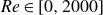
4. Role of longitudinal rolls
4.1. Thermally assisted sustaining process (TASP) in small domains,
$\varGamma = 2\pi$

Given the complex spatio-temporal dynamics of the newly identified intermittent rolls and the co-existence of longitudinal rolls with turbulent bands (see Appendices C.3 and C.4, respectively), we consider simulations in small domains defined by $\varGamma = 2\pi$
, where longitudinal rolls and localised turbulence could be viewed as spatially isolated. This domain size is chosen such that the spanwise wavelength of the most unstable longitudinal rolls (
$\varGamma = 2\pi$
, where longitudinal rolls and localised turbulence could be viewed as spatially isolated. This domain size is chosen such that the spanwise wavelength of the most unstable longitudinal rolls ( $\lambda _z\simeq \pi$
) is comparable to the horizontal length of the domain. Simulations for a smaller domain (
$\lambda _z\simeq \pi$
) is comparable to the horizontal length of the domain. Simulations for a smaller domain ( $\varGamma =\pi$
) do not show any qualitative difference from the simulation results reported here (Huang Reference Huang2025). We start from a numerical simulation at
$\varGamma =\pi$
) do not show any qualitative difference from the simulation results reported here (Huang Reference Huang2025). We start from a numerical simulation at $Ra = 10\,000$
and
$Ra = 10\,000$
and $\textit{Re}=1050$
in
$\textit{Re}=1050$
in $\varGamma = 2\pi$
, integrated in time for
$\varGamma = 2\pi$
, integrated in time for $t \in [0, 3000]$
. The initial condition has been sampled from a statistically stationary turbulent field at
$t \in [0, 3000]$
. The initial condition has been sampled from a statistically stationary turbulent field at $\textit{Re} = 2000$
for
$\textit{Re} = 2000$
for $Ra=10\,000$
, and the
$Ra=10\,000$
, and the $\textit{Re}$
is then slowly lowered to
$\textit{Re}$
is then slowly lowered to $\textit{Re} = 1050$
. The time history for
$\textit{Re} = 1050$
. The time history for $t \in [0, 3000]$
of the two near-wall transport properties, the Nusselt number and the shear rate on the lower wall is presented in figure 2, together with snapshots of the temperature,
$t \in [0, 3000]$
of the two near-wall transport properties, the Nusselt number and the shear rate on the lower wall is presented in figure 2, together with snapshots of the temperature, $\theta (\boldsymbol{x})$
, and the near-wall streamwise and spanwise perturbation velocities,
$\theta (\boldsymbol{x})$
, and the near-wall streamwise and spanwise perturbation velocities, $u'|_{y^+= 15}, v'|_{y^+=15}$
at selected times. In this small domain, the dynamics of the system exhibits temporal intermittency, where the solution trajectory appears to wander between longitudinal rolls and highly disorganised chaotic flow fields, characterised by low- and high-near-wall transport properties, respectively.
$u'|_{y^+= 15}, v'|_{y^+=15}$
at selected times. In this small domain, the dynamics of the system exhibits temporal intermittency, where the solution trajectory appears to wander between longitudinal rolls and highly disorganised chaotic flow fields, characterised by low- and high-near-wall transport properties, respectively.
Intermittent dynamics in a small domain at $Ra = 10000$
,
$Ra = 10000$
, $\textit{Re} = 1050$
,
$\textit{Re} = 1050$
, $t\in [0,3000]$
,
$t\in [0,3000]$
, $\varGamma = 2\pi$
. (a) The time history of the Nusselt number and shear. Temporal snapshots of volumetric temperature, planar near-wall streamwise and spanwise perturbations at (b)
$\varGamma = 2\pi$
. (a) The time history of the Nusselt number and shear. Temporal snapshots of volumetric temperature, planar near-wall streamwise and spanwise perturbations at (b) $t = 1291.5$
, (c)
$t = 1291.5$
, (c) $t = 1480.5$
, (d)
$t = 1480.5$
, (d) $t = 1564.5$
, (e)
$t = 1564.5$
, (e) $t = 1711.5$
. Longitudinal rolls and transient turbulence are observed in panels (b,d) and (c,e), respectively.
$t = 1711.5$
. Longitudinal rolls and transient turbulence are observed in panels (b,d) and (c,e), respectively.

Starting from a longitudinal roll state of spanwise wavenumber of $\alpha d = 4$
at
$\alpha d = 4$
at $t = 1291.5$
in figure 2(b), the solution erupts into a highly disorganised turbulent state at
$t = 1291.5$
in figure 2(b), the solution erupts into a highly disorganised turbulent state at $t = 1480.5$
, marked by a disordered temperature field in figure 2(c). During this breakdown, the near-wall snapshots of streamwise perturbation velocity,
$t = 1480.5$
, marked by a disordered temperature field in figure 2(c). During this breakdown, the near-wall snapshots of streamwise perturbation velocity, $u'|_{y^+ = 15}$
, and wall-normal perturbation velocity,
$u'|_{y^+ = 15}$
, and wall-normal perturbation velocity, $v'|_{y^+ = 15}$
, illustrated in the bottom panels of figure 2(c), reveal three pairs of high- and low-speed streaks, each with an average spanwise wavelength of
$v'|_{y^+ = 15}$
, illustrated in the bottom panels of figure 2(c), reveal three pairs of high- and low-speed streaks, each with an average spanwise wavelength of $\varLambda _z^+ \approx 339/3 = 113$
(where
$\varLambda _z^+ \approx 339/3 = 113$
(where $\varLambda _z^+ = u_\tau \varLambda _z / \nu$
refers to non-dimensionalised wavelength), close to the mean streak spacing (
$\varLambda _z^+ = u_\tau \varLambda _z / \nu$
refers to non-dimensionalised wavelength), close to the mean streak spacing ( $\varLambda ^+_z \sim 100$
) commonly reported in shear flow turbulence (Kline et al. Reference Kline, Reynolds, Schraub and Runstadler1967; Smith & Metzler Reference Smith and Metzler1983; Kim, Moin & Moser Reference Kim, Moin and Moser1987; Hamilton et al. Reference Hamilton, Kim and Waleffe1995). These streaks appear to be meandering, negatively correlated with wall-normal perturbation velocities, reminiscent of a streak breakdown process (Hamilton et al. Reference Hamilton, Kim and Waleffe1995), or a bursting event (Kim, Kline & Reynolds Reference Kim, Kline and Reynolds1971), where high- and low-speed streaks are brought close to and away from the wall, respectively, enhancing near-wall transport quantities. Indeed, this is reflected in large increments in the Nusselt number and wall shear rate of roughly
$\varLambda ^+_z \sim 100$
) commonly reported in shear flow turbulence (Kline et al. Reference Kline, Reynolds, Schraub and Runstadler1967; Smith & Metzler Reference Smith and Metzler1983; Kim, Moin & Moser Reference Kim, Moin and Moser1987; Hamilton et al. Reference Hamilton, Kim and Waleffe1995). These streaks appear to be meandering, negatively correlated with wall-normal perturbation velocities, reminiscent of a streak breakdown process (Hamilton et al. Reference Hamilton, Kim and Waleffe1995), or a bursting event (Kim, Kline & Reynolds Reference Kim, Kline and Reynolds1971), where high- and low-speed streaks are brought close to and away from the wall, respectively, enhancing near-wall transport quantities. Indeed, this is reflected in large increments in the Nusselt number and wall shear rate of roughly $40\,\%$
at
$40\,\%$
at $t = 1480.5$
in figure 2(a). Subsequently, the solution trajectory returns to a longitudinal roll state at
$t = 1480.5$
in figure 2(a). Subsequently, the solution trajectory returns to a longitudinal roll state at $t=1564.5$
, before erupting into turbulence at
$t=1564.5$
, before erupting into turbulence at $t = 1711.5$
(see figure 2
d,e, respectively). This suggests that the turbulence has a finite lifetime, occurring transiently before decaying towards the laminar state at
$t = 1711.5$
(see figure 2
d,e, respectively). This suggests that the turbulence has a finite lifetime, occurring transiently before decaying towards the laminar state at $\textit{Re} = 1050$
(Hof et al. Reference Hof, Westerweel, Schneider and Eckhardt2006; Schneider, Eckhardt & Yorke Reference Schneider, Eckhardt and Yorke2007), which is linearly unstable, leading to the onset of longitudinal rolls where transient turbulence could be re-excited again.
$\textit{Re} = 1050$
(Hof et al. Reference Hof, Westerweel, Schneider and Eckhardt2006; Schneider, Eckhardt & Yorke Reference Schneider, Eckhardt and Yorke2007), which is linearly unstable, leading to the onset of longitudinal rolls where transient turbulence could be re-excited again.
Relaminarisation in a small domain at $Ra = 0$
,
$Ra = 0$
, $\textit{Re} = 1050$
,
$\textit{Re} = 1050$
, $t\in [0,3000]$
,
$t\in [0,3000]$
, $\varGamma = 2\pi$
. The time history of the (a) Nusselt number and shear. Temporal snapshots of volumetric temperature at (b)
$\varGamma = 2\pi$
. The time history of the (a) Nusselt number and shear. Temporal snapshots of volumetric temperature at (b) $t = 31.5$
, (c)
$t = 31.5$
, (c) $t = 63$
, (d)
$t = 63$
, (d) $t = 157.5$
, (e)
$t = 157.5$
, (e) $t = 672$
.
$t = 672$
.

To test this hypothesis, we consider a numerical simulation at $Ra = 0$
,
$Ra = 0$
, $\textit{Re} = 1050$
, in
$\textit{Re} = 1050$
, in $\varGamma = 2\pi$
, where longitudinal rolls cannot appear. The initial condition is taken from a stationary turbulent solution at a higher
$\varGamma = 2\pi$
, where longitudinal rolls cannot appear. The initial condition is taken from a stationary turbulent solution at a higher $\textit{Re}$
of
$\textit{Re}$
of $\textit{Re} = 2000$
, which is then slowly lowered to
$\textit{Re} = 2000$
, which is then slowly lowered to $\textit{Re} = 1050$
and then integrated in time for
$\textit{Re} = 1050$
and then integrated in time for $t \in [0, 700]$
. The time history of the Nusselt number,
$t \in [0, 700]$
. The time history of the Nusselt number, $\textit{Nu}$
, and the wall shear rate,
$\textit{Nu}$
, and the wall shear rate, $\langle \tau _w \rangle _{x,z}$
, is reported in figure 3, with the temperature snapshots,
$\langle \tau _w \rangle _{x,z}$
, is reported in figure 3, with the temperature snapshots, $\theta (\boldsymbol{x})$
, at selected time units. An initial turbulent flow field decays towards the laminar solution in
$\theta (\boldsymbol{x})$
, at selected time units. An initial turbulent flow field decays towards the laminar solution in $t \in [0, 700]$
. Comparing the results between
$t \in [0, 700]$
. Comparing the results between $Ra = 0$
and
$Ra = 0$
and $Ra = 10\,000$
, we propose that the longitudinal rolls at
$Ra = 10\,000$
, we propose that the longitudinal rolls at $Ra= 10\,000$
could mediate a transition mechanism between the unstable laminar state and transient turbulence, so that the entire non-trivial flow dynamics could be sustained indefinitely.
$Ra= 10\,000$
could mediate a transition mechanism between the unstable laminar state and transient turbulence, so that the entire non-trivial flow dynamics could be sustained indefinitely.
Next, we investigate the impact of longitudinal rolls on this proposed mechanism at different $Ra$
. We capture the flow quantities for
$Ra$
. We capture the flow quantities for $Ra=10\,000$
and
$Ra=10\,000$
and $\textit{Re}=1050$
at
$\textit{Re}=1050$
at $t=850.5$
(just before the onset of longitudinal rolls, see figure 2), and use as an initial condition to perform four numerical simulations by lowering
$t=850.5$
(just before the onset of longitudinal rolls, see figure 2), and use as an initial condition to perform four numerical simulations by lowering $Ra$
instantly to
$Ra$
instantly to $Ra=8000,5000,3000,2000$
, and time-integrated further to
$Ra=8000,5000,3000,2000$
, and time-integrated further to $t \in [850.5, 5000]$
. The time history of the wall shear rate,
$t \in [850.5, 5000]$
. The time history of the wall shear rate, $\langle \tau _w\rangle _{x,z}$
, and the temperature snapshots,
$\langle \tau _w\rangle _{x,z}$
, and the temperature snapshots, $\theta (\boldsymbol{x})$
, of these experiments of ‘
$\theta (\boldsymbol{x})$
, of these experiments of ‘ $Ra$
-quenching’ are presented in figure 4. The time history of shear is visibly intermittent for
$Ra$
-quenching’ are presented in figure 4. The time history of shear is visibly intermittent for $Ra = 8000, 5000$
, depicted as the orange and green trajectories in figure 4(a), similar to
$Ra = 8000, 5000$
, depicted as the orange and green trajectories in figure 4(a), similar to $Ra = 10\,000$
. At
$Ra = 10\,000$
. At $Ra= 8000, 5000$
, the longitudinal rolls emerge approximately at
$Ra= 8000, 5000$
, the longitudinal rolls emerge approximately at $t = 1312.5$
(see figure 4
c,e), before erupting into turbulence at
$t = 1312.5$
(see figure 4
c,e), before erupting into turbulence at $t = 1743$
and
$t = 1743$
and $t = 3570$
in figure 4(d, f), respectively. This is then accompanied by a large spike in the wall shear rate before dipping briefly, shown as the orange and green trajectories of figure 4(a). As
$t = 3570$
in figure 4(d, f), respectively. This is then accompanied by a large spike in the wall shear rate before dipping briefly, shown as the orange and green trajectories of figure 4(a). As $Ra$
is lowered further to
$Ra$
is lowered further to $Ra = 3000, 2000$
, the transients begin to decay into a longitudinal state from
$Ra = 3000, 2000$
, the transients begin to decay into a longitudinal state from $t = 850.5$
to
$t = 850.5$
to $t = 1312.5$
, which remains stable until
$t = 1312.5$
, which remains stable until $t = 4200$
illustrated by figure 4(h, j), accompanied by the red and purple asymptotic trajectories in figure 4(a). This suggests that the longitudinal rolls are likely to be linearly unstable for
$t = 4200$
illustrated by figure 4(h, j), accompanied by the red and purple asymptotic trajectories in figure 4(a). This suggests that the longitudinal rolls are likely to be linearly unstable for $Ra = 8000, 5000$
, leading to turbulence, while remaining stable for
$Ra = 8000, 5000$
, leading to turbulence, while remaining stable for $Ra = 3000,2000$
. In particular, the longitudinal roll state at
$Ra = 3000,2000$
. In particular, the longitudinal roll state at $Ra = 5000$
remained saturated for a longer period
$Ra = 5000$
remained saturated for a longer period $t \in [1500, 3400]$
(green curve in figure 4
a), indicating that the growth rate of the linear instability is smaller than for
$t \in [1500, 3400]$
(green curve in figure 4
a), indicating that the growth rate of the linear instability is smaller than for $Ra = 8000$
. We note that the longitudinal rolls in figure 4 have a spanwise wavenumber of
$Ra = 8000$
. We note that the longitudinal rolls in figure 4 have a spanwise wavenumber of $\alpha d=4$
, which corresponds to the wavenumber of the dominant primary instability (see Appendix E), indicating that it is the most preferred wavenumber within a small domain.
$\alpha d=4$
, which corresponds to the wavenumber of the dominant primary instability (see Appendix E), indicating that it is the most preferred wavenumber within a small domain. $Ra$
-quenching experiments for
$Ra$
-quenching experiments for $Ra = 8000, 5000, 3000, 2000$
, at
$Ra = 8000, 5000, 3000, 2000$
, at $\textit{Re} = 1050$
,
$\textit{Re} = 1050$
, $\varGamma = 2\pi$
,
$\varGamma = 2\pi$
, $t \in [850.5, 5000]$
. The time history of (a) shear and (b) volumetric temperature snapshots of the flow condition at
$t \in [850.5, 5000]$
. The time history of (a) shear and (b) volumetric temperature snapshots of the flow condition at $t = 850.5$
. Volumetric temperature snapshots for
$t = 850.5$
. Volumetric temperature snapshots for $Ra = 8000$
at (c,d)
$Ra = 8000$
at (c,d) $t = 1312.5, 1743$
, and
$t = 1312.5, 1743$
, and $Ra = 5000$
at (e, f)
$Ra = 5000$
at (e, f) $t = 1312.5, 3570$
, revealing a longitudinal roll and a turbulent state, respectively. Stable longitudinal rolls emerge for
$t = 1312.5, 3570$
, revealing a longitudinal roll and a turbulent state, respectively. Stable longitudinal rolls emerge for $Ra = 3000$
at (g,h)
$Ra = 3000$
at (g,h) $t = 1312.5, 4200$
, and
$t = 1312.5, 4200$
, and $Ra = 2000$
at ( j,k)
$Ra = 2000$
at ( j,k) $t = 1312.5, 4200$
.
$t = 1312.5, 4200$
.

Growth rates of infinitesimal perturbations linearised about longitudinal rolls, $\boldsymbol{q}_{\textit{LR}}$
, of spanwise wavenumber of
$\boldsymbol{q}_{\textit{LR}}$
, of spanwise wavenumber of $\beta h = 2$
, against (a) streamwise wavenumber
$\beta h = 2$
, against (a) streamwise wavenumber $\alpha h$
and (b)
$\alpha h$
and (b) $Ra$
for
$Ra$
for $\alpha h =1$
. The hatches in panel (a) refer to wavenumbers smaller than those admissible in
$\alpha h =1$
. The hatches in panel (a) refer to wavenumbers smaller than those admissible in $\varGamma = 2\pi$
. The dash-dotted line in panel (b) is a standard quadratic regression yielding
$\varGamma = 2\pi$
. The dash-dotted line in panel (b) is a standard quadratic regression yielding $Ra_{s}\approx 4720$
.
$Ra_{s}\approx 4720$
.

To understand the stability characteristics of the longitudinal rolls, we perform a linear stability analysis about the longitudinal roll state ( $\alpha d= 4$
), at
$\alpha d= 4$
), at $Ra = 10\,000, 8000,{} 5000, 3000, 2000$
. The details of linear stability analysis are described in § 2.4, where
$Ra = 10\,000, 8000,{} 5000, 3000, 2000$
. The details of linear stability analysis are described in § 2.4, where $\lambda$
and
$\lambda$
and $\boldsymbol{\breve {q}}(y,z)e^{i\alpha x}$
refer to the eigenvalue and eigenmode. The longitudinal roll (base) states,
$\boldsymbol{\breve {q}}(y,z)e^{i\alpha x}$
refer to the eigenvalue and eigenmode. The longitudinal roll (base) states, $\boldsymbol{q}_{\textit{LR}}$
, are obtained by time integrating an initial condition consisting of the laminar (conduction) state, superimposed by the primary eigenmode,
$\boldsymbol{q}_{\textit{LR}}$
, are obtained by time integrating an initial condition consisting of the laminar (conduction) state, superimposed by the primary eigenmode, $\beta h = 2$
, at
$\beta h = 2$
, at $Ra = 10\,000, 8000, 5000, 3000, 2000$
, in a two-dimensional
$Ra = 10\,000, 8000, 5000, 3000, 2000$
, in a two-dimensional $y{-}z$
plane, suppressing any three-dimensional perturbations numerically. The growth rates as a function of discrete streamwise wavenumbers,
$y{-}z$
plane, suppressing any three-dimensional perturbations numerically. The growth rates as a function of discrete streamwise wavenumbers, $1 \leqslant \alpha h \leqslant 2.5$
, are presented in figure 5. We note that the admissible streamwise wavenumbers within
$1 \leqslant \alpha h \leqslant 2.5$
, are presented in figure 5. We note that the admissible streamwise wavenumbers within $\varGamma = 2\pi$
are
$\varGamma = 2\pi$
are $\alpha h = m$
, where
$\alpha h = m$
, where $m$
is a positive integer,
$m$
is a positive integer, $m = 1, 2, ..$
, and
$m = 1, 2, ..$
, and $\alpha h = 1.5, 2.5$
are included for completeness. The longitudinal rolls are linearly unstable for
$\alpha h = 1.5, 2.5$
are included for completeness. The longitudinal rolls are linearly unstable for $Ra \geqslant 5000$
, while they remain stable for
$Ra \geqslant 5000$
, while they remain stable for $Ra \leqslant 3000$
, which confirms our earlier hypothesis. In particular, the growth rates between
$Ra \leqslant 3000$
, which confirms our earlier hypothesis. In particular, the growth rates between $Ra = 5000$
and
$Ra = 5000$
and $Ra = 10\,000$
differ by an order of magnitude, which could explain the prolonged period of saturation in the green curve of figure 4(a). The dominant secondary instability of longitudinal rolls in
$Ra = 10\,000$
differ by an order of magnitude, which could explain the prolonged period of saturation in the green curve of figure 4(a). The dominant secondary instability of longitudinal rolls in $\varGamma = 2\pi$
has a streamwise wavenumber of
$\varGamma = 2\pi$
has a streamwise wavenumber of $\alpha h = 1$
. Using a standard quadratic regression, the critical Rayleigh number for disturbances with
$\alpha h = 1$
. Using a standard quadratic regression, the critical Rayleigh number for disturbances with $\alpha h = 1$
is approximately
$\alpha h = 1$
is approximately $Ra_{s} \approx 4720$
, presented in figure 5(b).
$Ra_{s} \approx 4720$
, presented in figure 5(b).
Time integration along the dominant unstable manifold, $\alpha h=1$
, of the longitudinal rolls at
$\alpha h=1$
, of the longitudinal rolls at $Ra = 5000, \textit{Re} = 1050,$ $\varGamma = 2\pi$
for
$\varGamma = 2\pi$
for $t\in [0,8000]$
. Time history of the (a) Nusselt number and wall shear rate, and (b) midplane temperature space–time plot. This system oscillates between the longitudinal rolls (
$t\in [0,8000]$
. Time history of the (a) Nusselt number and wall shear rate, and (b) midplane temperature space–time plot. This system oscillates between the longitudinal rolls ( $\textit{LR1}{-}4$
) and turbulence (
$\textit{LR1}{-}4$
) and turbulence ( $T1{-}4$
) over four intervals. Snapshots of temperature at (c)
$T1{-}4$
) over four intervals. Snapshots of temperature at (c) $t = 105$
, (d)
$t = 105$
, (d) $t = 1512$
, (e)
$t = 1512$
, (e) $t = 2446.5$
, ( f)
$t = 2446.5$
, ( f) $t = 2992.5$
, (g)
$t = 2992.5$
, (g) $t = 3727.5$
, (h)
$t = 3727.5$
, (h) $t = 5103$
, (i)
$t = 5103$
, (i) $t = 6300$
, (j)
$t = 6300$
, (j) $t = 6993$
.
$t = 6993$
.

Following this, we examine the dominant unstable manifold ( $\alpha h = 1$
) of the longitudinal rolls (
$\alpha h = 1$
) of the longitudinal rolls ( $\beta h = 2$
) at
$\beta h = 2$
) at $Ra=5000$
, by considering an initial condition,
$Ra=5000$
, by considering an initial condition,
 \begin{equation} \boldsymbol{q}_0(\boldsymbol{x},t=0) = \boldsymbol{q}_{\textit{LR}}(y,z) + \boldsymbol{\breve {q}}(y,z)e^{i\alpha x}+c.c. \end{equation}
Here, $\breve {\boldsymbol{q}} e^{i \alpha x}$
is an eigenmode for the streamwise wavenumber
$\breve {\boldsymbol{q}} e^{i \alpha x}$
is an eigenmode for the streamwise wavenumber $\alpha$
and its amplitude was scaled such that its total energy is defined by
$\alpha$
and its amplitude was scaled such that its total energy is defined by
 \begin{equation} \delta = \frac {1}{{V}} \int _\varOmega \Bigg (\boldsymbol{\hat {u}}(\boldsymbol{x})^T\boldsymbol{\hat {u}}(\boldsymbol{x}) + \frac {Ra}{8\textit{Re}^2\textit{Pr}}\hat {\theta }(\boldsymbol{x})^2 \Bigg )\; \mathrm{d}\varOmega = 10^{-3}. \end{equation}
We have also considered that $\delta = 10^{-2}, 10^{-4}$
, but
$\delta = 10^{-2}, 10^{-4}$
, but $\delta = 10^{-3}$
was found to be small enough to ensure linear growth, while large enough without requiring a large number of time steps.
$\delta = 10^{-3}$
was found to be small enough to ensure linear growth, while large enough without requiring a large number of time steps.
The initial condition is time-integrated for $t \in [0, 8000]$
and its time history of the near-wall transport properties, the space–time plot of the mid-plane temperature,
$t \in [0, 8000]$
and its time history of the near-wall transport properties, the space–time plot of the mid-plane temperature, $\theta |_{(x,y)=(\pi ,0)}$
, are presented in figure 6, with snapshots of temperature,
$\theta |_{(x,y)=(\pi ,0)}$
, are presented in figure 6, with snapshots of temperature, $\theta (\boldsymbol{x})$
, and near-wall streamwise and spanwise perturbation velocities,
$\theta (\boldsymbol{x})$
, and near-wall streamwise and spanwise perturbation velocities, $u'|_{y^+= 15}$
,
$u'|_{y^+= 15}$
, $v'|_{y^+=15}$
at some selected times. The intermittent trajectory is visually apparent, oscillating between longitudinal rolls and transient turbulence over four cycles for
$v'|_{y^+=15}$
at some selected times. The intermittent trajectory is visually apparent, oscillating between longitudinal rolls and transient turbulence over four cycles for $t \in [0, 8000]$
: for example, the regions of low and high near-wall transport quantities in figure 6(a) correspond well to the organised and disorganised longitudinal rolls in figure 6(b), respectively. As the solution emerges from the unstable manifold of the longitudinal roll state,
$t \in [0, 8000]$
: for example, the regions of low and high near-wall transport quantities in figure 6(a) correspond well to the organised and disorganised longitudinal rolls in figure 6(b), respectively. As the solution emerges from the unstable manifold of the longitudinal roll state, $(\textit{LR1})$
in figure 6(c), the trajectory erupts into turbulence at
$(\textit{LR1})$
in figure 6(c), the trajectory erupts into turbulence at $t = 1512$
, marked by a disordered volumetric temperature field in snapshot
$t = 1512$
, marked by a disordered volumetric temperature field in snapshot $(T1)$
in figure 6(d). Turbulence occurs transiently and the solution decays towards a longitudinal roll-like state at
$(T1)$
in figure 6(d). Turbulence occurs transiently and the solution decays towards a longitudinal roll-like state at $t = 2446.5$
, shown by snapshot
$t = 2446.5$
, shown by snapshot $(\textit{LR2})$
in figure 6(e), forming a single cycle. The intermittent cycle repeats over three subsequent intervals, where the transient turbulent state and longitudinal rolls emerge at
$(\textit{LR2})$
in figure 6(e), forming a single cycle. The intermittent cycle repeats over three subsequent intervals, where the transient turbulent state and longitudinal rolls emerge at $t = 2992.5, 5103, 6993$
and
$t = 2992.5, 5103, 6993$
and $t = 3727.5, 6300$
, as shown in the snapshots
$t = 3727.5, 6300$
, as shown in the snapshots $(T2,3,4)$
and
$(T2,3,4)$
and $(\textit{LR3},4)$
in figures 6( f,h, j) and 6(g,i), respectively. Lastly, here, we show that the dominant unstable manifold of the longitudinal rolls is connected to a transient turbulent state. Interestingly, a longitudinal roll with
$(\textit{LR3},4)$
in figures 6( f,h, j) and 6(g,i), respectively. Lastly, here, we show that the dominant unstable manifold of the longitudinal rolls is connected to a transient turbulent state. Interestingly, a longitudinal roll with $\beta h = 1$
sometimes emerges after turbulence decays, shown as the snapshot
$\beta h = 1$
sometimes emerges after turbulence decays, shown as the snapshot $(\textit{LR3})$
. This suggests that other unstable manifolds may well be linked to the transition to transient turbulence.
$(\textit{LR3})$
. This suggests that other unstable manifolds may well be linked to the transition to transient turbulence.
State space projection based on the planar averaged centreline velocity and shear, coloured by the volume normalised perturbation kinetic energy at $Ra = 5000$
,
$Ra = 5000$
, $\textit{Re} = 1050$
,
$\textit{Re} = 1050$
, $\varGamma = 2\pi$
, (a)
$\varGamma = 2\pi$
, (a) $t \in [0,800]$
, (b)
$t \in [0,800]$
, (b) $t \in [0, 68750]$
. The open black circles represent the unstable equilibria of longitudinal rolls and the laminar state. Note that the black-crosses, labelled by (T1–4) and (LR1–4), refer to temporal snapshots in figure 6, not equilibria solutions.
$t \in [0, 68750]$
. The open black circles represent the unstable equilibria of longitudinal rolls and the laminar state. Note that the black-crosses, labelled by (T1–4) and (LR1–4), refer to temporal snapshots in figure 6, not equilibria solutions.

To better visualise the temporal dynamics in figure 6, we project the solution trajectory onto the space composed of two state observables: planar averaged centreline velocity, $\langle u|_{y=0} \rangle _{x,z}$
, the wall shear rate,
$\langle u|_{y=0} \rangle _{x,z}$
, the wall shear rate, $\langle \tau _w\rangle _{x,z}$
, coloured by the volume-averaged perturbation kinetic energy,
$\langle \tau _w\rangle _{x,z}$
, coloured by the volume-averaged perturbation kinetic energy, $1/(2V)||\boldsymbol{u}'||^2$
, in figure 7, where
$1/(2V)||\boldsymbol{u}'||^2$
, in figure 7, where $\|\boldsymbol{u}'\|^2=\int _\varOmega \boldsymbol{u}'^H\boldsymbol{u}' \,{\rm d}V$
with
$\|\boldsymbol{u}'\|^2=\int _\varOmega \boldsymbol{u}'^H\boldsymbol{u}' \,{\rm d}V$
with $\varOmega$
being the flow domain. These observables are chosen because they are found to distinguish well the regions of turbulent states, longitudinal roll states and the laminar state that reside around
$\varOmega$
being the flow domain. These observables are chosen because they are found to distinguish well the regions of turbulent states, longitudinal roll states and the laminar state that reside around $(0.82, 3.2)$
,
$(0.82, 3.2)$
, $(0.90, 2.32)$
and at
$(0.90, 2.32)$
and at $(1, 2)$
, respectively. Indeed, the temporal snapshots of
$(1, 2)$
, respectively. Indeed, the temporal snapshots of $(T1{-}4)$
appear around the representative location of turbulent states,
$(T1{-}4)$
appear around the representative location of turbulent states, $(0.82, 3.2)$
, and the snapshots of
$(0.82, 3.2)$
, and the snapshots of $(\textit{LR1}{-}4)$
and an equilibrium related to the longitudinal roll state with the spanwise wavenumber
$(\textit{LR1}{-}4)$
and an equilibrium related to the longitudinal roll state with the spanwise wavenumber $\beta h=2$
(denoted by
$\beta h=2$
(denoted by $\boldsymbol{q}_{\textit{LR}, \beta h = 2}$
) are seen around
$\boldsymbol{q}_{\textit{LR}, \beta h = 2}$
) are seen around $(0.90, 2.32)$
.
$(0.90, 2.32)$
.
The solution trajectory emerges from the unstable manifold of the longitudinal roll state, $\boldsymbol{q}_{\textit{LR}_{\beta h = 2}}$
, evolving towards turbulent states around
$\boldsymbol{q}_{\textit{LR}_{\beta h = 2}}$
, evolving towards turbulent states around $(0.85,3.2)$
, characterised by a high wall shear rate. At this
$(0.85,3.2)$
, characterised by a high wall shear rate. At this $\textit{Re}$
, the turbulence is transient in small domains, occurring with a finite lifetime, eventually decaying towards the laminar state (Zammert & Eckhardt Reference Zammert and Eckhardt2015; Tuckerman et al. Reference Tuckerman, Chantry and Barkley2020; Paranjape et al. Reference Paranjape, Yalnız, Duguet, Budanur and Hof2023). As the solution trajectory approaches the laminar solution at
$\textit{Re}$
, the turbulence is transient in small domains, occurring with a finite lifetime, eventually decaying towards the laminar state (Zammert & Eckhardt Reference Zammert and Eckhardt2015; Tuckerman et al. Reference Tuckerman, Chantry and Barkley2020; Paranjape et al. Reference Paranjape, Yalnız, Duguet, Budanur and Hof2023). As the solution trajectory approaches the laminar solution at $(1,2)$
, it abruptly reverses towards the longitudinal roll state near
$(1,2)$
, it abruptly reverses towards the longitudinal roll state near $(0.95, 2.15)$
,
$(0.95, 2.15)$
, $(\textit{LR3})$
, due to the buoyancy-driven linear instability of the laminar base state in the RBP flow. Subsequently, the solution trajectory could depart along an unstable manifold of the longitudinal rolls again, forming a cyclic process.
$(\textit{LR3})$
, due to the buoyancy-driven linear instability of the laminar base state in the RBP flow. Subsequently, the solution trajectory could depart along an unstable manifold of the longitudinal rolls again, forming a cyclic process.
To see if this cycle could be sustained indefinitely, we consider a longer time horizon, $t \in [0, 68750]$
, illustrated in figure 7(b). The solution trajectory wanders between the ‘cloud’ of transient turbulence at the top left corner (in red), and longitudinal roll and laminar states (in blue) in the bottom right, forming a basin of attraction between the unstable longitudinal rolls, transient turbulence and the unstable laminar base state. This basin of attraction is likely established above a critical
$t \in [0, 68750]$
, illustrated in figure 7(b). The solution trajectory wanders between the ‘cloud’ of transient turbulence at the top left corner (in red), and longitudinal roll and laminar states (in blue) in the bottom right, forming a basin of attraction between the unstable longitudinal rolls, transient turbulence and the unstable laminar base state. This basin of attraction is likely established above a critical $Ra$
as the longitudinal rolls become linearly unstable (i.e.
$Ra$
as the longitudinal rolls become linearly unstable (i.e. $Ra \gtrsim Ra_{s} \approx 4720$
, see figure 5
b) and the instability of the longitudinal rolls provides an intermediate pathway towards transient turbulence, which could be regenerated again – a ‘self-sustaining’ dynamical process. We refer to this process as the thermally assisted sustaining process (TASP), inspired by the self-sustaining process (SSP) from turbulent shear flows (Hamilton et al. Reference Hamilton, Kim and Waleffe1995). A schematic of the TASP is illustrated in figure 8.
$Ra \gtrsim Ra_{s} \approx 4720$
, see figure 5
b) and the instability of the longitudinal rolls provides an intermediate pathway towards transient turbulence, which could be regenerated again – a ‘self-sustaining’ dynamical process. We refer to this process as the thermally assisted sustaining process (TASP), inspired by the self-sustaining process (SSP) from turbulent shear flows (Hamilton et al. Reference Hamilton, Kim and Waleffe1995). A schematic of the TASP is illustrated in figure 8.
Thermally assisted sustaining process (TASP).

4.2. Variation of
$Ra$
and
$\textit{Re}$
on the TASP in small domains,
$\varGamma = 2\pi$


Behaviour of the unstable and stable longitudinal rolls at $Ra = 8000, 4000$
for (a,e)
$Ra = 8000, 4000$
for (a,e) $\textit{Re} = 600$
, (b, f)
$\textit{Re} = 600$
, (b, f) $\textit{Re} = 700$
, (c,g)
$\textit{Re} = 700$
, (c,g) $\textit{Re} = 1000$
and (d,h)
$\textit{Re} = 1000$
and (d,h) $\textit{Re} = 1400$
within
$\textit{Re} = 1400$
within $\varGamma = 2\pi$
. Each parameter regime consist of three panels from the top to bottom, depicting the midplane temperature space–time plot,
$\varGamma = 2\pi$
. Each parameter regime consist of three panels from the top to bottom, depicting the midplane temperature space–time plot, $\theta |_{(x,y) = ( \pi ,0)}$
, time history of the Nusselt number and shear, and state space projection based on the planar averaged centreline velocity and shear, coloured by the volume normalised perturbation kinetic energy.
$\theta |_{(x,y) = ( \pi ,0)}$
, time history of the Nusselt number and shear, and state space projection based on the planar averaged centreline velocity and shear, coloured by the volume normalised perturbation kinetic energy.

In this section, we further explore the behaviour of the TASP as $\textit{Re}$
and
$\textit{Re}$
and $Ra$
are varied. We consider eight different cases at
$Ra$
are varied. We consider eight different cases at $Ra = 8000, 4000$
and
$Ra = 8000, 4000$
and $\textit{Re} = 600, 700, 1000, 1400$
. The results of these eight cases, where longitudinal rolls are unstable at
$\textit{Re} = 600, 700, 1000, 1400$
. The results of these eight cases, where longitudinal rolls are unstable at $Ra = 8000$
or stable at
$Ra = 8000$
or stable at $Ra = 4000$
, are shown in figure 9, depicting the space–time plots of the midplane temperature,
$Ra = 4000$
, are shown in figure 9, depicting the space–time plots of the midplane temperature, $\theta |_{y=0}(x,t)$
, the time history of the Nusselt number,
$\theta |_{y=0}(x,t)$
, the time history of the Nusselt number, $\textit{Nu}$
, and the wall shear rate,
$\textit{Nu}$
, and the wall shear rate, $\langle \tau _w \rangle _{x,z}$
, and the state space portrait using the plane-averaged centreline velocity,
$\langle \tau _w \rangle _{x,z}$
, and the state space portrait using the plane-averaged centreline velocity, $\langle u|_{y=0} \rangle _{x,z}$
, the wall shear rate. For all cases, except
$\langle u|_{y=0} \rangle _{x,z}$
, the wall shear rate. For all cases, except $Ra = 4000$
,
$Ra = 4000$
, $\textit{Re} = 1000$
and
$\textit{Re} = 1000$
and $\textit{Re} = 1400$
, their initial conditions are prepared from the laminar state, superimposed by a random noise based on a Gaussian distribution with zero mean and unit variance, scaled to a total energy of
$\textit{Re} = 1400$
, their initial conditions are prepared from the laminar state, superimposed by a random noise based on a Gaussian distribution with zero mean and unit variance, scaled to a total energy of $\delta = 10^{-3}$
(see (4.2) for the definition). For the exceptional cases at
$\delta = 10^{-3}$
(see (4.2) for the definition). For the exceptional cases at $Ra = 4000$
,
$Ra = 4000$
, $\textit{Re} = 1000$
and
$\textit{Re} = 1000$
and $\textit{Re} = 1400$
, where subcritical turbulence and stable longitudinal rolls are expected, their initial conditions are obtained by gradually lowering
$\textit{Re} = 1400$
, where subcritical turbulence and stable longitudinal rolls are expected, their initial conditions are obtained by gradually lowering $\textit{Re}$
from a statistically stationary turbulent solution at
$\textit{Re}$
from a statistically stationary turbulent solution at $Ra = 4000, \textit{Re} = 2000$
.
$Ra = 4000, \textit{Re} = 2000$
.
We first consider $\textit{Re}=1000$
(figure 9
c,g). At
$\textit{Re}=1000$
(figure 9
c,g). At $Ra = 8000$
(figure 9
c), the trajectory visits transient turbulence near
$Ra = 8000$
(figure 9
c), the trajectory visits transient turbulence near $t=7200$
, decaying towards the longitudinal roll state,
$t=7200$
, decaying towards the longitudinal roll state, $\boldsymbol{q}_{\textit{LR}}$
with roll wavenumber
$\boldsymbol{q}_{\textit{LR}}$
with roll wavenumber $\beta h =2$
, at
$\beta h =2$
, at $t = 7400$
, before regenerating again, consistent with the TASP in § 4.1. As
$t = 7400$
, before regenerating again, consistent with the TASP in § 4.1. As $Ra$
is lowered to
$Ra$
is lowered to $4000$
(figure 9
g), the solution trajectory decays towards the longitudinal roll state,
$4000$
(figure 9
g), the solution trajectory decays towards the longitudinal roll state, $\boldsymbol{q}_{\textit{LR}}$
. In this case, the longitudinal rolls are linearly stable, confirming our hypothesis earlier that the TASP is only established when longitudinal rolls become linearly unstable above a certain
$\boldsymbol{q}_{\textit{LR}}$
. In this case, the longitudinal rolls are linearly stable, confirming our hypothesis earlier that the TASP is only established when longitudinal rolls become linearly unstable above a certain $Ra$
-threshold (i.e.
$Ra$
-threshold (i.e. $Ra \gtrsim Ra_{s} \approx 4720$
).
$Ra \gtrsim Ra_{s} \approx 4720$
).
At $\textit{Re} = 1400$
,
$\textit{Re} = 1400$
, $Ra = 4000$
, the solution trajectory remains within the turbulent ‘cloud’ near
$Ra = 4000$
, the solution trajectory remains within the turbulent ‘cloud’ near $(0.8, 3.8)$
for
$(0.8, 3.8)$
for $t \in [0,10000]$
, as illustrated in figure 9(h). This suggests that turbulence in this case might be an attractor sustaining indefinitely, although we have not investigated whether the turbulent chaotic saddle at
$t \in [0,10000]$
, as illustrated in figure 9(h). This suggests that turbulence in this case might be an attractor sustaining indefinitely, although we have not investigated whether the turbulent chaotic saddle at $\textit{Re} = 1000$
truly transitioned into an attractor at
$\textit{Re} = 1000$
truly transitioned into an attractor at $\textit{Re} = 1400$
. As
$\textit{Re} = 1400$
. As $Ra$
is increased to
$Ra$
is increased to $8000$
, the solution trajectory originating from the laminar state, evolves towards the unstable longitudinal roll state,
$8000$
, the solution trajectory originating from the laminar state, evolves towards the unstable longitudinal roll state, $\boldsymbol{q}_{\textit{LR}}$
at
$\boldsymbol{q}_{\textit{LR}}$
at $t = 1550$
, transitioning into turbulence at
$t = 1550$
, transitioning into turbulence at $t= 1800$
. Therefore, in this case, the linearly unstable longitudinal rolls serve as an intermediate transitional pathway between the laminar base state and subcritical turbulence, whereas at
$t= 1800$
. Therefore, in this case, the linearly unstable longitudinal rolls serve as an intermediate transitional pathway between the laminar base state and subcritical turbulence, whereas at $Ra = 4000$
, a bistability between stable longitudinal rolls (not shown) and turbulence is expected.
$Ra = 4000$
, a bistability between stable longitudinal rolls (not shown) and turbulence is expected.
Next, we examine the behaviour of TASP as $\textit{Re}$
decreases towards the intermittent regime at
$\textit{Re}$
decreases towards the intermittent regime at $\textit{Re} = 600, 700$
, where a periodic orbit emerges between the longitudinal roll and the laminar state (figure 9
a,b,e, f). At
$\textit{Re} = 600, 700$
, where a periodic orbit emerges between the longitudinal roll and the laminar state (figure 9
a,b,e, f). At $\textit{Re} = 600, Ra = 8000$
in figure 9(a), the solution trajectory initially evolves towards the longitudinal roll state,
$\textit{Re} = 600, Ra = 8000$
in figure 9(a), the solution trajectory initially evolves towards the longitudinal roll state, $\boldsymbol{q}_{\textit{LR}}$
, which is linearly unstable and breaks down towards the laminar state at
$\boldsymbol{q}_{\textit{LR}}$
, which is linearly unstable and breaks down towards the laminar state at $t = 2200$
. This breakdown is evidenced by the trajectory’s proximity to the laminar state in state space and the presence of a narrow green patch in the midplane temperature space–time plot. The longitudinal roll state is regenerated again, forming a periodic orbit with a period of
$t = 2200$
. This breakdown is evidenced by the trajectory’s proximity to the laminar state in state space and the presence of a narrow green patch in the midplane temperature space–time plot. The longitudinal roll state is regenerated again, forming a periodic orbit with a period of $T_{\textit{period}} = 8098-6108 =1990$
, oscillating between the longitudinal roll and laminar state over five intervals within
$T_{\textit{period}} = 8098-6108 =1990$
, oscillating between the longitudinal roll and laminar state over five intervals within $t \in [0, 10\,000]$
. As
$t \in [0, 10\,000]$
. As $\textit{Re}$
increases slightly to
$\textit{Re}$
increases slightly to $700$
, the periodic orbit persists over a shorter period of
$700$
, the periodic orbit persists over a shorter period of $T_{\textit{period}} = 3889 - 3386 = 503$
. A notable difference is observed in the regenerated longitudinal rolls, which is continuously translated by
$T_{\textit{period}} = 3889 - 3386 = 503$
. A notable difference is observed in the regenerated longitudinal rolls, which is continuously translated by $L_z/2$
in the spanwise
$L_z/2$
in the spanwise $z$
-direction. Additionally, as
$z$
-direction. Additionally, as $\textit{Re}$
increases from
$\textit{Re}$
increases from $600$
to
$600$
to $700$
, the trajectory moves further away from the laminar state during breakdown, suggesting an increasing attraction towards the longitudinal roll state,
$700$
, the trajectory moves further away from the laminar state during breakdown, suggesting an increasing attraction towards the longitudinal roll state, $\boldsymbol{q}_{\textit{LR}}$
(compare
$\boldsymbol{q}_{\textit{LR}}$
(compare $t = 2200$
in figure 9
a and
$t = 2200$
in figure 9
a and $t = 2750$
in figure 9
b). When
$t = 2750$
in figure 9
b). When $Ra$
is lowered to
$Ra$
is lowered to $Ra = 4000$
, the periodic orbit disappears and the trajectory stabilises into the longitudinal roll state,
$Ra = 4000$
, the periodic orbit disappears and the trajectory stabilises into the longitudinal roll state, $\boldsymbol{q}_{\textit{LR}}$
, at
$\boldsymbol{q}_{\textit{LR}}$
, at $\textit{Re} = 600, 700$
(figure 9
e, f).
$\textit{Re} = 600, 700$
(figure 9
e, f).
A state space sketch of figure 9 at $Ra = 8000$
, (a)
$Ra = 8000$
, (a) $\textit{Re} = 600$
, (b)
$\textit{Re} = 600$
, (b) $\textit{Re} = 700$
, (c)
$\textit{Re} = 700$
, (c) $\textit{Re} = 1000$
, (d)
$\textit{Re} = 1000$
, (d) $\textit{Re} = 1400$
and
$\textit{Re} = 1400$
and $Ra = 4000$
at (e)
$Ra = 4000$
at (e) $\textit{Re} = 600,700$
, ( f)
$\textit{Re} = 600,700$
, ( f) $\textit{Re} = 1000$
, (g)
$\textit{Re} = 1000$
, (g) $\textit{Re} =1400$
. The longitudinal roll is linearly unstable (saddle) at
$\textit{Re} =1400$
. The longitudinal roll is linearly unstable (saddle) at $Ra = 8000$
and is stable at
$Ra = 8000$
and is stable at $Ra = 4000$
, whereas the laminar state is always linearly unstable (saddle). The blue and orange solid arrows refer to the unstable manifold of longitudinal rolls and the laminar state. The red solid lines denote the chaotic trajectories of turbulence, likely forming a chaotic saddle at
$Ra = 4000$
, whereas the laminar state is always linearly unstable (saddle). The blue and orange solid arrows refer to the unstable manifold of longitudinal rolls and the laminar state. The red solid lines denote the chaotic trajectories of turbulence, likely forming a chaotic saddle at $\textit{Re} = 1000$
and a chaotic attractor at
$\textit{Re} = 1000$
and a chaotic attractor at $\textit{Re} = 1400$
. The black-dashed trajectories refer to possible solution trajectories, forming a periodic orbit (P.O) at
$\textit{Re} = 1400$
. The black-dashed trajectories refer to possible solution trajectories, forming a periodic orbit (P.O) at $Ra = 8000$
,
$Ra = 8000$
, $\textit{Re} = 600, 700$
, and a basin of attraction (B.o.A) at
$\textit{Re} = 600, 700$
, and a basin of attraction (B.o.A) at $Ra = 8000, \textit{Re} = 1000$
. We note that invariant states could exist at
$Ra = 8000, \textit{Re} = 1000$
. We note that invariant states could exist at $Ra = 4000, \textit{Re} = 600,700$
, labelled as a saddle here (Paranjape et al. Reference Paranjape, Yalnız, Duguet, Budanur and Hof2023).
$Ra = 4000, \textit{Re} = 600,700$
, labelled as a saddle here (Paranjape et al. Reference Paranjape, Yalnız, Duguet, Budanur and Hof2023).

To summarise the dynamical processes identified in figure 9, we present their state space sketch in figure 10. At $Ra = 8000$
,
$Ra = 8000$
, $\textit{Re} = 600$
and
$\textit{Re} = 600$
and $\textit{Re}= 700$
, the longitudinal rolls become linearly unstable, breaking down to the laminar state before being regenerated, forming a periodic orbit enclosed by black dotted paths in figure 10(a,b). For
$\textit{Re}= 700$
, the longitudinal rolls become linearly unstable, breaking down to the laminar state before being regenerated, forming a periodic orbit enclosed by black dotted paths in figure 10(a,b). For $\textit{Re} = 700$
, the regenerated longitudinal roll is continuously translated by
$\textit{Re} = 700$
, the regenerated longitudinal roll is continuously translated by $L_z/2$
, suggesting a possible merger of two periodic orbits into one as sketched in figure 9(b). Future bifurcation studies are required to establish this, providing an avenue for future work. As
$L_z/2$
, suggesting a possible merger of two periodic orbits into one as sketched in figure 9(b). Future bifurcation studies are required to establish this, providing an avenue for future work. As $Ra$
is lowered to
$Ra$
is lowered to $Ra = 4000$
, the laminar state stabilises into the longitudinal rolls in figure 10(e). However, the flow in this regime may contain some invariant solutions (e.g. see Paranjape et al. Reference Paranjape, Yalnız, Duguet, Budanur and Hof2023), denoted as saddle points here. Integrating along the unstable manifold of longitudinal roll states at
$Ra = 4000$
, the laminar state stabilises into the longitudinal rolls in figure 10(e). However, the flow in this regime may contain some invariant solutions (e.g. see Paranjape et al. Reference Paranjape, Yalnız, Duguet, Budanur and Hof2023), denoted as saddle points here. Integrating along the unstable manifold of longitudinal roll states at $Ra= 8000, \textit{Re} = 1000$
leads to transient turbulence, which eventually decays to the laminar state before regenerating the longitudinal rolls again, forming the TASP in figure 10(c). In contrast, at
$Ra= 8000, \textit{Re} = 1000$
leads to transient turbulence, which eventually decays to the laminar state before regenerating the longitudinal rolls again, forming the TASP in figure 10(c). In contrast, at $Ra = 4000, \textit{Re} = 1000$
, the longitudinal rolls become linearly stable, eliminating the intermediate (orange) pathway towards turbulence. Therefore, the transient turbulence stabilises into longitudinal rolls, as shown by the black-dashed trajectory in figure 10( f). For
$Ra = 4000, \textit{Re} = 1000$
, the longitudinal rolls become linearly stable, eliminating the intermediate (orange) pathway towards turbulence. Therefore, the transient turbulence stabilises into longitudinal rolls, as shown by the black-dashed trajectory in figure 10( f). For $Ra = 8000, \textit{Re} = 1400$
, the linearly unstable longitudinal rolls provide an intermediate pathway towards turbulence from the laminar state, as sketched in figure 10(d), breaking the bistability between the laminar state and subcritical turbulence seen at
$Ra = 8000, \textit{Re} = 1400$
, the linearly unstable longitudinal rolls provide an intermediate pathway towards turbulence from the laminar state, as sketched in figure 10(d), breaking the bistability between the laminar state and subcritical turbulence seen at $Ra = 4000$
in figure 10(g). This difference highlights the contribution of unstable longitudinal rolls towards the transition to turbulence within
$Ra = 4000$
in figure 10(g). This difference highlights the contribution of unstable longitudinal rolls towards the transition to turbulence within $\varGamma = 2\pi$
.
$\varGamma = 2\pi$
.
We have examined the dynamics of unstable longitudinal rolls, as the Reynolds number, $\textit{Re}$
, and the Rayleigh number,
$\textit{Re}$
, and the Rayleigh number, $Ra$
, are varied, identifying three key dynamical processes: (1) periodic orbits between longitudinal rolls and the laminar state (figure 10
a,b); (2) the TASP, where transient turbulence can be sustained (figure 10
c); and (3) an intermediate transitional pathway towards sustained turbulence (figure 10
d). To establish a connection between these processes and refine their transitional boundaries, we conduct a further parametric study over fifteen numerical simulations at
$Ra$
, are varied, identifying three key dynamical processes: (1) periodic orbits between longitudinal rolls and the laminar state (figure 10
a,b); (2) the TASP, where transient turbulence can be sustained (figure 10
c); and (3) an intermediate transitional pathway towards sustained turbulence (figure 10
d). To establish a connection between these processes and refine their transitional boundaries, we conduct a further parametric study over fifteen numerical simulations at $Ra = 4000, 6000, 10\,000$
and
$Ra = 4000, 6000, 10\,000$
and $\textit{Re} = 600, 800, 900, 1200, 1400$
for
$\textit{Re} = 600, 800, 900, 1200, 1400$
for $\varGamma = 2\pi$
. Figure 11 presents the midplane temperature space–time plot along with the time history of the wall shear rate,
$\varGamma = 2\pi$
. Figure 11 presents the midplane temperature space–time plot along with the time history of the wall shear rate, $\langle \tau _w\rangle _{x,z}$
, and the Nusselt number,
$\langle \tau _w\rangle _{x,z}$
, and the Nusselt number, $\textit{Nu}$
. For all simulations, the initial conditions are prepared from the laminar state, superimposed with a random noise based on a Gaussian distribution with zero mean and unit variance, scaled to a total energy of
$\textit{Nu}$
. For all simulations, the initial conditions are prepared from the laminar state, superimposed with a random noise based on a Gaussian distribution with zero mean and unit variance, scaled to a total energy of $\delta = 10^{-3}$
(see definition in (4.2)). Due to the subcritical nature of turbulence and expected stable longitudinal rolls, exceptions are made for
$\delta = 10^{-3}$
(see definition in (4.2)). Due to the subcritical nature of turbulence and expected stable longitudinal rolls, exceptions are made for $Ra = 4000$
,
$Ra = 4000$
, $\textit{Re} = 900, 1200, 1400$
, where initial conditions are taken from gradually lowering
$\textit{Re} = 900, 1200, 1400$
, where initial conditions are taken from gradually lowering $\textit{Re}$
from a statistically stationary turbulent state at
$\textit{Re}$
from a statistically stationary turbulent state at $Ra = 4000, \textit{Re} = 2000$
. The thermally assisted sustaining process is highlighted in green for
$Ra = 4000, \textit{Re} = 2000$
. The thermally assisted sustaining process is highlighted in green for $Ra \in [6000, 10\,000]$
and
$Ra \in [6000, 10\,000]$
and $\textit{Re} \in [900, 1200]$
, where temporally intermittent shear and Nusselt number fluctuations are observed, accompanied by a mixture of organised and disorganised flow structures in the temperature space–time plots. Here, longitudinal rolls provide an intermediate pathway towards transient turbulence. For the same
$\textit{Re} \in [900, 1200]$
, where temporally intermittent shear and Nusselt number fluctuations are observed, accompanied by a mixture of organised and disorganised flow structures in the temperature space–time plots. Here, longitudinal rolls provide an intermediate pathway towards transient turbulence. For the same $\textit{Re}$
and as
$\textit{Re}$
and as $Ra$
lowers to
$Ra$
lowers to $4000$
, transient turbulence eventually decays into stable longitudinal rolls labelled as ‘transient turbulence’ in figure 11. Periodic and quasi-periodic orbits between longitudinal rolls and the laminar state appear for
$4000$
, transient turbulence eventually decays into stable longitudinal rolls labelled as ‘transient turbulence’ in figure 11. Periodic and quasi-periodic orbits between longitudinal rolls and the laminar state appear for $Ra = 10000$
,
$Ra = 10000$
, $\textit{Re} = 600, 800$
and
$\textit{Re} = 600, 800$
and $Ra = 6000$
,
$Ra = 6000$
, $\textit{Re} = 800$
, establishing threshold values of
$\textit{Re} = 800$
, establishing threshold values of $Ra$
and
$Ra$
and $\textit{Re}$
shaded in yellow. Below this threshold, solutions stabilise into longitudinal rolls shaded in red. Although longitudinal rolls are linearly stable at
$\textit{Re}$
shaded in yellow. Below this threshold, solutions stabilise into longitudinal rolls shaded in red. Although longitudinal rolls are linearly stable at $Ra = 4000, \textit{Re} = 1400$
, turbulence is sustained at least for a sufficiently long time, shaded blue at
$Ra = 4000, \textit{Re} = 1400$
, turbulence is sustained at least for a sufficiently long time, shaded blue at $\textit{Re} = 1400$
and labelled as ‘sustained turbulence’ in figure 11. In this case, a bistable system forms between longitudinal rolls and turbulence at
$\textit{Re} = 1400$
and labelled as ‘sustained turbulence’ in figure 11. In this case, a bistable system forms between longitudinal rolls and turbulence at $Ra = 4000$
, while longitudinal rolls provide an intermediate pathway to turbulence for
$Ra = 4000$
, while longitudinal rolls provide an intermediate pathway to turbulence for $Ra \geqslant 6000$
.
$Ra \geqslant 6000$
.
Finally, we aim to establish the relevance of the local dynamical processes, such as the TASP identified in the small domain simulations of this section, to the results obtained in large domain simulations (see § 3), as discussed in Appendix D.
Temperature space–time plots and time history of $(\tau _w, Nu)$
, for
$(\tau _w, Nu)$
, for $Ra \in [5000, 10\,000]$
,
$Ra \in [5000, 10\,000]$
, $\textit{Re} \in [600, 1400]$
within
$\textit{Re} \in [600, 1400]$
within $\varGamma = 2\pi$
. Unstable longitudinal rolls lead to the onset of (1) periodic orbits (yellow), (2) the thermally assisted sustaining process (green) and (3) sustained turbulence (blue), occurring beyond an
$\varGamma = 2\pi$
. Unstable longitudinal rolls lead to the onset of (1) periodic orbits (yellow), (2) the thermally assisted sustaining process (green) and (3) sustained turbulence (blue), occurring beyond an $Ra{-}\textit{Re}$
boundary, below which longitudinal rolls remain stable (red).
$Ra{-}\textit{Re}$
boundary, below which longitudinal rolls remain stable (red).

5. Conclusions
We conclude by summarising the key findings of the transitional RBP flow in figure 1, where we have identified five distinct regimes and their rough transition boundaries. At low $\textit{Re}$
, the flow structures are primarily organised by buoyancy-driven convection rolls, consistent with RBC studies, including features such as the bistability between ISRs and SDC, and the secondary oscillatory instability. We have shown that SDC disappears in the range
$\textit{Re}$
, the flow structures are primarily organised by buoyancy-driven convection rolls, consistent with RBC studies, including features such as the bistability between ISRs and SDC, and the secondary oscillatory instability. We have shown that SDC disappears in the range $0.1 \lt \textit{Re} \lt 1$
, and the critical
$0.1 \lt \textit{Re} \lt 1$
, and the critical $\textit{Re}$
at which this occurs warrants further investigation. At intermediate
$\textit{Re}$
at which this occurs warrants further investigation. At intermediate $\textit{Re}$
, we identify a new regime known as intermittent rolls, marked by the breakdown and regeneration of longitudinal rolls. As
$\textit{Re}$
, we identify a new regime known as intermittent rolls, marked by the breakdown and regeneration of longitudinal rolls. As $\textit{Re}$
approaches the onset of shear-driven turbulence, we observe the co-existence of longitudinal rolls with turbulent–laminar bands. This highlights the importance of longitudinal rolls in spatially extended RBP flows. By considering a small domain, we showed that the linearly unstable longitudinal rolls could provide a transition mechanism towards turbulence, referred to as the thermally assisted sustaining process (TASP). Finally, we examined how TASP evolves as
$\textit{Re}$
approaches the onset of shear-driven turbulence, we observe the co-existence of longitudinal rolls with turbulent–laminar bands. This highlights the importance of longitudinal rolls in spatially extended RBP flows. By considering a small domain, we showed that the linearly unstable longitudinal rolls could provide a transition mechanism towards turbulence, referred to as the thermally assisted sustaining process (TASP). Finally, we examined how TASP evolves as $Ra$
and
$Ra$
and $\textit{Re}$
are varied, and discuss its implications for spatially extended domains. Further work may include a bifurcation analysis study of the TASP within small domains and minimal band unit, establishing dynamical connections between invariant solutions where large spatial intermittency structures are expected to be important in the transitional regime (Tuckerman et al. Reference Tuckerman, Chantry and Barkley2020).
$\textit{Re}$
are varied, and discuss its implications for spatially extended domains. Further work may include a bifurcation analysis study of the TASP within small domains and minimal band unit, establishing dynamical connections between invariant solutions where large spatial intermittency structures are expected to be important in the transitional regime (Tuckerman et al. Reference Tuckerman, Chantry and Barkley2020).
We note that the development of longitudinal and wavy rolls is convectively unstable (Carrière & Monkewitz Reference Carrière and Monkewitz1999; Pabiou et al. Reference Pabiou, Mergui and Bénard2005). Therefore, if a localised small impulsive disturbance is introduced around the laminar basic state in an infinitely extended spatial domain, it is expected that the complex transition dynamics involving the intermittent rolls will be washed out from the given domain of interest after some time. Therefore, to observe this regime, a controlled excitation of noise to the system would need to be provided upstream (Pabiou et al. Reference Pabiou, Mergui and Bénard2005; Nicolas et al. Reference Nicolas, Zoueidi and Xin2012), and this was also how spatio-temporally intermittent turbulence is measured experimentally in pipe flows undergoing a subcritical transition (e.g. see Avila et al. Reference Avila, Moxey, de Lozar, Avila, Barkley and Hof2011).
Finally, we discuss the TASP in relation to other transitional shear flow phenomena in the absence of buoyancy force, such as intermittent puffs in pipe flows (Avila et al. Reference Avila, Barkley and Hof2023), turbulent–laminar bands in plane Couette and Poiseuille flows (Tuckerman et al. Reference Tuckerman, Chantry and Barkley2020), and the self-sustaining process (Hamilton et al. Reference Hamilton, Kim and Waleffe1995). The TASP primarily relies on a buoyancy-driven linear instability of the laminar state and the subsequent secondary instability of the resulting longitudinal rolls to reach a turbulent state that can be relaminarised at any time due to its nature of being a ‘chaotic saddle’ at low Reynolds numbers. By nature, the entire quasi-cyclic dynamics of TASP forms a chaotic attractor encompassing both laminar and turbulent states, although the turbulent state observed intermittently remains a chaotic saddle locally in the state space. In contrast, the onset of turbulent puffs and turbulent–laminar bands is subcritical and requires finite-amplitude perturbations. The SSP is the underlying physical mechanism supporting turbulent puffs and bands, but, around the onset of turbulent dynamics, it forms a chaotic saddle through a ‘crisis’ bifurcation (e.g. Kreilos & Eckhardt Reference Kreilos and Eckhardt2012; Zammert & Eckhardt Reference Zammert and Eckhardt2015).
Despite the fundamental difference between TASP and SSP in the geometrical structure in the state space, it should be mentioned that the longitudinal rolls emerging through a linear instability in TASP involve the amplification of streaks, as the rolls created by the buoyancy force initiate the lift-up effect (Jerome et al. Reference Jerome, Chomaz and Huerre2012). The process of reaching a turbulent state through the subsequent secondary instability of the longitudinal rolls is also similar to the streak instability or transient growth in SSP – indeed, the presence of meandering streaks (see figure 2
c) is reminiscent of the streak breakdown phase in SSP. This suggests that the chaotic dynamics between TASP and SSP may well occur in a synchronised manner, although this does not always appear to be the case. For example, the time scale of TASP is seen to be much longer than that of typical SSP, since the flow can almost be relaminarised (see figure 6). Furthermore, it should be noted that the small domain considered in the present study is roughly twice as wide ( $L_z^+ \approx 339$
) as that of the SSP in a minimal flow unit (Hamilton et al. Reference Hamilton, Kim and Waleffe1995, e.g.
$L_z^+ \approx 339$
) as that of the SSP in a minimal flow unit (Hamilton et al. Reference Hamilton, Kim and Waleffe1995, e.g. $L_z^+ \approx 116.9 - 143.6$
). Therefore, a natural extension of this work would be to investigate exactly when and how TASP and SSP possibly interact in transitional and fully developed turbulent flows.
$L_z^+ \approx 116.9 - 143.6$
). Therefore, a natural extension of this work would be to investigate exactly when and how TASP and SSP possibly interact in transitional and fully developed turbulent flows.
Acknowledgements
C.H.C. gratefully acknowledges the funding received from the Imperial College President’s Ph.D. scholarship. The authors would like to thank EPSRC for the computational time made available on the UK supercomputing facility ARCHER/ARCHER2 via the UK Turbulence Consortium (EP/X035484/1).
Declaration of interests
The authors report no conflict of interest.
Appendix A. Governing equations for Rayleigh–Bénard convection
The governing equations for Rayleigh–Bénard convection are the non-dimensionalised equations with the Boussinesq approximation for buoyancy-driven flow, given by
 \begin{equation} \frac {\partial \boldsymbol{u}}{\partial t} + (\boldsymbol{u} \boldsymbol{\cdot }\boldsymbol{\nabla }) \boldsymbol{u} = -\boldsymbol{\nabla }\!p + \textit{Pr}{\nabla} ^2 \boldsymbol{u} + \frac {\textit{RaPr}}{8}\theta \boldsymbol{{j}}, \end{equation}
 \begin{equation} \frac {\partial \theta }{\partial t} + (\boldsymbol{u} \boldsymbol{\cdot }\boldsymbol{\nabla }) \theta ={\nabla} ^2 \theta , \end{equation}
 \begin{equation} \boldsymbol{\nabla }\boldsymbol{\cdot }\boldsymbol{u} = 0, \end{equation}
subjected to the following boundary conditions at the walls:
 \begin{equation} \boldsymbol{u}|_{y=\pm 1} = 0, \quad \theta |_{y=-1} = 1, \quad \theta |_{y=1} = 0, \end{equation}
and the periodic boundary conditions imposed in the planar $x$
and
$x$
and $z$
directions. Here,
$z$
directions. Here, $t$
denotes the time scaled by the vertical thermal diffusion time,
$t$
denotes the time scaled by the vertical thermal diffusion time, $d^2/\kappa$
, and
$d^2/\kappa$
, and $\boldsymbol{x}(=(x,y,z))$
represents the spatial coordinates non-dimensionalised by depth,
$\boldsymbol{x}(=(x,y,z))$
represents the spatial coordinates non-dimensionalised by depth, $2h$
The horizontal directions are
$2h$
The horizontal directions are $x$
and
$x$
and $z$
, while
$z$
, while $y$
is the vertical direction. The velocity vector is given by
$y$
is the vertical direction. The velocity vector is given by $\boldsymbol{u}(=(u,v,w))$
and is scaled by thermal velocity,
$\boldsymbol{u}(=(u,v,w))$
and is scaled by thermal velocity, $\kappa /d$
. The pressure
$\kappa /d$
. The pressure $p$
is scaled by
$p$
is scaled by $ \rho \kappa ^2 / d^2$
, while
$ \rho \kappa ^2 / d^2$
, while $\theta (\equiv (T-T_U)/\Delta T)$
refers to the non-dimensional temperature with
$\theta (\equiv (T-T_U)/\Delta T)$
refers to the non-dimensional temperature with $T$
being the absolute temperature, and
$T$
being the absolute temperature, and $\boldsymbol{j}$
denotes the unit vector in
$\boldsymbol{j}$
denotes the unit vector in $y$
-direction. The Rayleigh number,
$y$
-direction. The Rayleigh number, $Ra$
, and the Prandtl number,
$Ra$
, and the Prandtl number, $\textit{Pr}$
, are defined as in § 1. In this study, we set
$\textit{Pr}$
, are defined as in § 1. In this study, we set $\textit{Pr} = 1$
.
$\textit{Pr} = 1$
.
Summary of the spatial and temporal resolution for a given $\textit{Re}$
,
$\textit{Re}$
, $Ra$
.
$Ra$
. $N_z$
denotes the number of Fourier expansions in the
$N_z$
denotes the number of Fourier expansions in the $z$
-direction,
$z$
-direction, ${\rm d}t$
and
${\rm d}t$
and $\zeta$
denote the time step size and the final time, respectively.
$\zeta$
denote the time step size and the final time, respectively.

Appendix B. Simulation parameters for
$\textit{Ra}$
–
$\textit{Re}$
sweep


The spectral/hp quadrilateral element width, heights and polynomial order are kept constant for all simulations, $(\Delta x, \Delta y|_{y=\pm h}, \Delta y|_{y=0}, P) = (0.1\pi ,0.0549,0.367,4)$
. To resolve the high gradients, the quadrilateral element heights are bunched near the wall,
$(\Delta x, \Delta y|_{y=\pm h}, \Delta y|_{y=0}, P) = (0.1\pi ,0.0549,0.367,4)$
. To resolve the high gradients, the quadrilateral element heights are bunched near the wall, $\Delta y|_{y=\pm h}$
, and expanded in the channel centre,
$\Delta y|_{y=\pm h}$
, and expanded in the channel centre, $\Delta y|_{y=0}$
. The basis type employed here consists of the modified Jacobi polynomials, known as the modified basis (Karniadakis & Sherwin Reference Karniadakis and Sherwin2005). Table 1 describes the number of Fourier expansions,
$\Delta y|_{y=0}$
. The basis type employed here consists of the modified Jacobi polynomials, known as the modified basis (Karniadakis & Sherwin Reference Karniadakis and Sherwin2005). Table 1 describes the number of Fourier expansions, $N_z$
, and temporal resolution of 52 numerical experiments at
$N_z$
, and temporal resolution of 52 numerical experiments at $\textit{Re} = 0, 0.1, 1, 10, 100, 500, 750, 1000, 1050$
,
$\textit{Re} = 0, 0.1, 1, 10, 100, 500, 750, 1000, 1050$
, $2000$
and
$2000$
and $Ra = 0, 2000, 3000, 5000, 8000, 10\,000$
with
$Ra = 0, 2000, 3000, 5000, 8000, 10\,000$
with $\textit{Pr} = 1$
, and a large aspect ratio,
$\textit{Pr} = 1$
, and a large aspect ratio, $\varGamma = 16\pi$
. The initial conditions of all numerical experiments were sampled from a statistically stationary solution based on the time history of the Nusselt number and shear. The laminar solution obtained for
$\varGamma = 16\pi$
. The initial conditions of all numerical experiments were sampled from a statistically stationary solution based on the time history of the Nusselt number and shear. The laminar solution obtained for $Ra = 0$
,
$Ra = 0$
, $\textit{Re} \leqslant 1000$
has been omitted in table 1.
$\textit{Re} \leqslant 1000$
has been omitted in table 1.
Appendix C. Flow structures in large domains within the
$\boldsymbol{Ra}$
–
$\textit{Re}$
phase space


Here, we provide a detailed analysis of the flow structures identified in the $Ra$
–
$Ra$
– $\textit{Re}$
phase space presented in figure 1.
$\textit{Re}$
phase space presented in figure 1.
C.1. Buoyancy dominant regime
In the buoyancy-dominated regime, the flow structures are predominantly organised with convection rolls, such as SDC, transverse, oblique, longitudinal rolls (and ISRs with no mean flow) or oscillatory rolls. The bistability between SDC and ISRs is preserved for $Ra \geqslant 3000$
at
$Ra \geqslant 3000$
at $\textit{Re} = 0.1$
(refer to figure 12
a) and
$\textit{Re} = 0.1$
(refer to figure 12
a) and $\textit{Re} = 1$
for
$\textit{Re} = 1$
for $Ra \geqslant 5000$
(see also figure 14
a,d,g). There exists a maximum
$Ra \geqslant 5000$
(see also figure 14
a,d,g). There exists a maximum $\textit{Re}$
, beyond which SDC disappears; we denote this as
$\textit{Re}$
, beyond which SDC disappears; we denote this as $\textit{Re}_s$
and its dependence on
$\textit{Re}_s$
and its dependence on $Ra$
is demarcated by the black dashed lines on the left side of figure 1.
$Ra$
is demarcated by the black dashed lines on the left side of figure 1.
Midplane temperature snapshots at $Ra = 3000$
, (a)
$Ra = 3000$
, (a) $\textit{Re} = 0.1$
, (b)
$\textit{Re} = 0.1$
, (b) $\textit{Re} = 1$
, (c)
$\textit{Re} = 1$
, (c) $\textit{Re} = 10$
, (d)
$\textit{Re} = 10$
, (d) $\textit{Re} = 100$
, (e)
$\textit{Re} = 100$
, (e) $\textit{Re} = 500$
, ( f)
$\textit{Re} = 500$
, ( f) $\textit{Re} = 1000$
.
$\textit{Re} = 1000$
.

Wall-normal distribution of temporal and plane-averaged (a) streamwise velocity, (b) temperature, (c) fluctuating wall-normal velocity squared normalised by thermal velocity scale, (d) fluctuating temperature squared, and (e) fluctuating stream- and spanwise velocities squared normalised by thermal velocity scale of the buoyancy-driven regime (see the shaded red zone in figure 1). Note: the symbols ( $\star , \bullet , \blacktriangle$
) together with the coloured lines correspond to the respective combination of
$\star , \bullet , \blacktriangle$
) together with the coloured lines correspond to the respective combination of $\textit{Re}$
and
$\textit{Re}$
and $Ra$
.
$Ra$
.

Notably, an oblique roll with a ‘hooked-like’ defect is observed at $\textit{Re} = 1$
,
$\textit{Re} = 1$
, $Ra = 3000$
, shown in figure 12(b), reminiscent of the multiple ‘non-ISR’ states in RBC (see references in § 1.2). At
$Ra = 3000$
, shown in figure 12(b), reminiscent of the multiple ‘non-ISR’ states in RBC (see references in § 1.2). At $\textit{Re} = 10$
, the SDC disappears and longitudinal rolls with a spanwise wavenumber of
$\textit{Re} = 10$
, the SDC disappears and longitudinal rolls with a spanwise wavenumber of $\alpha d = 2.5$
emerge, illustrated in figure 12(c), suggesting that the roll wavenumber adheres to the stability boundaries of the Busse balloon (see also figure 6 of Bodenschatz et al. Reference Bodenschatz, Pesch and Ahlers2000). As
$\alpha d = 2.5$
emerge, illustrated in figure 12(c), suggesting that the roll wavenumber adheres to the stability boundaries of the Busse balloon (see also figure 6 of Bodenschatz et al. Reference Bodenschatz, Pesch and Ahlers2000). As $\textit{Re}$
is increased further to
$\textit{Re}$
is increased further to $1000$
, the longitudinal rolls emerge as the preferred solution at
$1000$
, the longitudinal rolls emerge as the preferred solution at $Ra = 2000, 3000$
. The non-dimensionalised spanwise wavenumber of longitudinal rolls observed at
$Ra = 2000, 3000$
. The non-dimensionalised spanwise wavenumber of longitudinal rolls observed at $Ra = 3000$
and
$Ra = 3000$
and $\textit{Re} = 100, 500, 10\,000$
, shown in figure 12(d–f), respectively, is approximately
$\textit{Re} = 100, 500, 10\,000$
, shown in figure 12(d–f), respectively, is approximately $\beta d \approx 3.3$
, which lies outside of the stability boundaries of the Busse balloon in RBC (figure 6 of Bodenschatz et al. Reference Bodenschatz, Pesch and Ahlers2000). This suggests that the stability boundaries of the longitudinal rolls may change as
$\beta d \approx 3.3$
, which lies outside of the stability boundaries of the Busse balloon in RBC (figure 6 of Bodenschatz et al. Reference Bodenschatz, Pesch and Ahlers2000). This suggests that the stability boundaries of the longitudinal rolls may change as $\textit{Re}$
increases. Interestingly, a stable ‘pinched’ longitudinal roll pattern emerges at
$\textit{Re}$
increases. Interestingly, a stable ‘pinched’ longitudinal roll pattern emerges at $\textit{Re} = 100$ $Ra = 3000$
, reminiscent of a skew-varicosed instability shown in figure 12(d). Unlike the secondary skewed-varicose instability observed in RBC, which reduces the wavenumber of an unstable ISR, by pinching adjacent rolls together, stabilising into a stable ISR (Bodenschatz et al. Reference Bodenschatz, Pesch and Ahlers2000, see figure 7), a stable ‘pinched’ tertiary state emerges here. Finally, we present the first- and second-order statistics of the buoyancy-dominated regime (shaded in red), consisting of the (1) SDC and ISRs, and (2) ISRs states in figure 13, illustrating its temporal and plane-averaged streamwise velocity,
$Ra = 3000$
, reminiscent of a skew-varicosed instability shown in figure 12(d). Unlike the secondary skewed-varicose instability observed in RBC, which reduces the wavenumber of an unstable ISR, by pinching adjacent rolls together, stabilising into a stable ISR (Bodenschatz et al. Reference Bodenschatz, Pesch and Ahlers2000, see figure 7), a stable ‘pinched’ tertiary state emerges here. Finally, we present the first- and second-order statistics of the buoyancy-dominated regime (shaded in red), consisting of the (1) SDC and ISRs, and (2) ISRs states in figure 13, illustrating its temporal and plane-averaged streamwise velocity, $\langle u \rangle _{x,z,t}$
, temperature,
$\langle u \rangle _{x,z,t}$
, temperature, $\langle \theta \rangle _{x,z,t}$
, fluctuating wall-normal velocity squared normalised by thermal velocity scale,
$\langle \theta \rangle _{x,z,t}$
, fluctuating wall-normal velocity squared normalised by thermal velocity scale, $\langle \tilde {v} \tilde {v} \rangle _{x,z,t}/u_\kappa ^2$
, fluctuating temperature squared,
$\langle \tilde {v} \tilde {v} \rangle _{x,z,t}/u_\kappa ^2$
, fluctuating temperature squared, $\langle \tilde {\theta }\tilde {\theta } \rangle _{x,z,t}$
, and fluctuating stream- and spanwise velocities squared normalised by thermal velocity scale,
$\langle \tilde {\theta }\tilde {\theta } \rangle _{x,z,t}$
, and fluctuating stream- and spanwise velocities squared normalised by thermal velocity scale, $\langle \tilde {u}\tilde {u} + \tilde {w}\tilde {w} \rangle _{x,z,t}/u_\kappa ^2$
. We note that the fluctuating components are defined about a temporal-planar averaged quantity, i.e.
$\langle \tilde {u}\tilde {u} + \tilde {w}\tilde {w} \rangle _{x,z,t}/u_\kappa ^2$
. We note that the fluctuating components are defined about a temporal-planar averaged quantity, i.e. $\tilde {\boldsymbol{u}} = \boldsymbol{u} - \langle \boldsymbol{u} \rangle _{x,z,t}$
. The mean temperature profiles (figure 13
b), and the fluctuating span- and streamwise velocities (figure 13
e) are visually similar for the same
$\tilde {\boldsymbol{u}} = \boldsymbol{u} - \langle \boldsymbol{u} \rangle _{x,z,t}$
. The mean temperature profiles (figure 13
b), and the fluctuating span- and streamwise velocities (figure 13
e) are visually similar for the same $Ra$
and are nearly independent of
$Ra$
and are nearly independent of $\textit{Re}$
. However, we observe the dependence on
$\textit{Re}$
. However, we observe the dependence on $\textit{Re}$
at
$\textit{Re}$
at $Ra = 3000$
in the fluctuating temperature squared (figure 13
d) and fluctuating wall-normal velocities (figure 13
c), likely due to variations in convection structures, particularly in the convection roll wavenumbers. A detailed analysis of how the statistical properties vary with roll wavenumber is beyond the scope of this work. We propose that the underlying flow structure, consisting of convection rolls, describes the buoyancy-driven regime, shaded in red in figure 1. In this regime, the strength of the convection is primarily controlled by
$Ra = 3000$
in the fluctuating temperature squared (figure 13
d) and fluctuating wall-normal velocities (figure 13
c), likely due to variations in convection structures, particularly in the convection roll wavenumbers. A detailed analysis of how the statistical properties vary with roll wavenumber is beyond the scope of this work. We propose that the underlying flow structure, consisting of convection rolls, describes the buoyancy-driven regime, shaded in red in figure 1. In this regime, the strength of the convection is primarily controlled by $Ra$
, akin to RBC, and remains independent of
$Ra$
, akin to RBC, and remains independent of $\textit{Re}$
.
$\textit{Re}$
.
C.2. Transition from the buoyancy regime to the mixed regime
Figure 14 presents a detailed analysis of the coarse-grained transition boundaries between SDC and ISRs in the range $\textit{Re} \in [1, 10]$
, and from ISRs to wavy rolls for
$\textit{Re} \in [1, 10]$
, and from ISRs to wavy rolls for $\textit{Re} \in [10, 100]$
across the high Rayleigh numbers considered,
$\textit{Re} \in [10, 100]$
across the high Rayleigh numbers considered, $Ra \in [5000, 10\,000]$
. As
$Ra \in [5000, 10\,000]$
. As $\textit{Re}$
increases from
$\textit{Re}$
increases from $1$
to
$1$
to $10$
, the SDC regime (see figure 14
a,d,g) vanishes and longitudinal rolls emerge, as shown in figure 14(b,e,h) for
$10$
, the SDC regime (see figure 14
a,d,g) vanishes and longitudinal rolls emerge, as shown in figure 14(b,e,h) for $Ra = 10\,000, 8000, 5000$
, respectively. These longitudinal rolls may undergo short-wavelength modulations, indicative of the secondary oscillatory instability of RBC occurring above
$Ra = 10\,000, 8000, 5000$
, respectively. These longitudinal rolls may undergo short-wavelength modulations, indicative of the secondary oscillatory instability of RBC occurring above $Ra \gt 5000$
(Clever & Busse Reference Clever and Busse1974). This results in the development of oscillatory longitudinal rolls described by a relative periodic orbit at
$Ra \gt 5000$
(Clever & Busse Reference Clever and Busse1974). This results in the development of oscillatory longitudinal rolls described by a relative periodic orbit at $Ra= 8000$
and a chaotic state at
$Ra= 8000$
and a chaotic state at $Ra = 10000$
, shown in figure 14(e,b), respectively. The footprint of oscillatory convection rolls is also evident in the SDC regime at
$Ra = 10000$
, shown in figure 14(e,b), respectively. The footprint of oscillatory convection rolls is also evident in the SDC regime at $Ra = 10000$
,
$Ra = 10000$
, $\textit{Re} = 1$
, shown in figure 14(a). As
$\textit{Re} = 1$
, shown in figure 14(a). As $\textit{Re}$
increases from
$\textit{Re}$
increases from $10$
to
$10$
to $100$
, the longitudinal rolls exhibit longer wavelength modulations, indicative of the wavy instability (Clever & Busse Reference Clever and Busse1991; Pabiou et al. Reference Pabiou, Mergui and Bénard2005). This gives rise to wavy longitudinal rolls, appearing as a travelling wave, quasi-periodic tori and a chaotic state at
$100$
, the longitudinal rolls exhibit longer wavelength modulations, indicative of the wavy instability (Clever & Busse Reference Clever and Busse1991; Pabiou et al. Reference Pabiou, Mergui and Bénard2005). This gives rise to wavy longitudinal rolls, appearing as a travelling wave, quasi-periodic tori and a chaotic state at $Ra = 5000, 8000, 10\,000$
, respectively, shown in figure 14(i, f,c), respectively. The wavelengths of the streamwise waviness and the spanwise periodic longitudinal roll appear to be approximately three intervals of streamwise length,
$Ra = 5000, 8000, 10\,000$
, respectively, shown in figure 14(i, f,c), respectively. The wavelengths of the streamwise waviness and the spanwise periodic longitudinal roll appear to be approximately three intervals of streamwise length, $\varLambda _x \sim L_x/3$
, and twelve intervals of spanwise length,
$\varLambda _x \sim L_x/3$
, and twelve intervals of spanwise length, $\varLambda _z \sim L_z/12$
, respectively.
$\varLambda _z \sim L_z/12$
, respectively.
Space–time plots of midplane temperature field, temperature snapshot and phase space trajectories of the Nusselt number against wall shear rate at: (a,b,c) $Ra = 10000$
for
$Ra = 10000$
for $\textit{Re} = 1, 10, 100$
; (d,e, f)
$\textit{Re} = 1, 10, 100$
; (d,e, f) $Ra = 8000$
for
$Ra = 8000$
for $\textit{Re} = 1,10,100$
; and (g,h,i)
$\textit{Re} = 1,10,100$
; and (g,h,i) $Ra = 5000$
for
$Ra = 5000$
for $\textit{Re} = 1, 10, 100$
. The flow patterns are primarily organised into spiral defect chaos, longitudinal rolls and wavy rolls occuring at
$\textit{Re} = 1, 10, 100$
. The flow patterns are primarily organised into spiral defect chaos, longitudinal rolls and wavy rolls occuring at $\textit{Re} = 1, 10, 100$
, respectively.
$\textit{Re} = 1, 10, 100$
, respectively.

C.3. Spatio-temporal intermittent rolls in large domains,
$\varGamma = 16\pi$

As $\textit{Re}$
approaches
$\textit{Re}$
approaches $\textit{Re} = 500$
, the wavy rolls disappear. Instead, a new regime, referred to as intermittent rolls, is observed. In this regime, the longitudinal rolls remain as the dominant convection structure, interspersed with a spatio-temporal intermittent breakdown towards the laminar state. This behaviour is illustrated for
$\textit{Re} = 500$
, the wavy rolls disappear. Instead, a new regime, referred to as intermittent rolls, is observed. In this regime, the longitudinal rolls remain as the dominant convection structure, interspersed with a spatio-temporal intermittent breakdown towards the laminar state. This behaviour is illustrated for $(Ra,\textit{Re}) = (8000,500$
) in figure 15(a) using the temporal oscillations of the plane-averaged shear rate on the lower wall,
$(Ra,\textit{Re}) = (8000,500$
) in figure 15(a) using the temporal oscillations of the plane-averaged shear rate on the lower wall, $\langle \tau _w \rangle _{x,z}$
, and the Nusselt number,
$\langle \tau _w \rangle _{x,z}$
, and the Nusselt number, $\textit{Nu}$
. We note
$\textit{Nu}$
. We note $\tau _w = 2$
and
$\tau _w = 2$
and $\textit{Nu} = 1$
for the laminar solution. The spatio-temporal intermittent breakdown of the longitudinal rolls towards the laminar state is observed in figure 15(b), where the bright and dark regions in the space–time plot of near-wall spanwise and wall-normal perturbation kinetic energy (
$\textit{Nu} = 1$
for the laminar solution. The spatio-temporal intermittent breakdown of the longitudinal rolls towards the laminar state is observed in figure 15(b), where the bright and dark regions in the space–time plot of near-wall spanwise and wall-normal perturbation kinetic energy ( $\mathcal{E}_{v'+w'} = 1/2(v'^2+ w'^2)$
) at
$\mathcal{E}_{v'+w'} = 1/2(v'^2+ w'^2)$
) at $(x,y^+)=(8\pi ,15)$
highlight the co-existence of longitudinal rolls and spatially localised laminar states; here,
$(x,y^+)=(8\pi ,15)$
highlight the co-existence of longitudinal rolls and spatially localised laminar states; here, $\boldsymbol{u}' = \boldsymbol{u} - U_{\textit{lam}}(y)$
and
$\boldsymbol{u}' = \boldsymbol{u} - U_{\textit{lam}}(y)$
and $y^+ = (y+1)/\textit{Re}_\tau$
with
$y^+ = (y+1)/\textit{Re}_\tau$
with $\textit{Re}_\tau =u_\tau h/\nu$
, where
$\textit{Re}_\tau =u_\tau h/\nu$
, where $u_\tau$
is the friction velocity. A similar observation is made with the space–time plot of midplane temperature,
$u_\tau$
is the friction velocity. A similar observation is made with the space–time plot of midplane temperature, $\theta |_{(x,y)=(8\pi ,0)}$
, in figure 15(c), where the elongated red/blue contours correspond to up-/down-welling regions of longitudinal rolls, and the green regions indicate spatially localised laminar states. The two near-wall transport properties, the wall shear rate and the Nusselt number exhibit strong correlations. For example, at
$\theta |_{(x,y)=(8\pi ,0)}$
, in figure 15(c), where the elongated red/blue contours correspond to up-/down-welling regions of longitudinal rolls, and the green regions indicate spatially localised laminar states. The two near-wall transport properties, the wall shear rate and the Nusselt number exhibit strong correlations. For example, at $t = 3736$
, both peaks reveal a spatially coherent longitudinal roll structure in figure 15(d,e). There are also dips observed at
$t = 3736$
, both peaks reveal a spatially coherent longitudinal roll structure in figure 15(d,e). There are also dips observed at $t = 6189$
and
$t = 6189$
and $t=8680$
, indicative of the spatially local breakdown towards the laminar state, as shown in figures 15( f,g) and 15(h,i), respectively. In summary, the longitudinal rolls enhance heat and momentum transfer towards the walls, but they appear to be intermittently disrupted by the breakdown towards the laminar state. To better understand this behaviour, we later consider the temporal dynamics in a small domain,
$t=8680$
, indicative of the spatially local breakdown towards the laminar state, as shown in figures 15( f,g) and 15(h,i), respectively. In summary, the longitudinal rolls enhance heat and momentum transfer towards the walls, but they appear to be intermittently disrupted by the breakdown towards the laminar state. To better understand this behaviour, we later consider the temporal dynamics in a small domain, $\varGamma = 2\pi$
, where the spatial intermittency is artificially suppressed (see § 4).
$\varGamma = 2\pi$
, where the spatial intermittency is artificially suppressed (see § 4).
Intermittent rolls regime at $Ra = 8000, \textit{Re} = 500$
,
$Ra = 8000, \textit{Re} = 500$
, $t \in [0, 10000]$
. (a) Time history of shear on the lower wall and Nusselt number. Space–time (
$t \in [0, 10000]$
. (a) Time history of shear on the lower wall and Nusselt number. Space–time ( $z$
–
$z$
– $t$
) plots of (b) near-wall wall-normal and spanwise perturbation kinetic energy, and (c) midplane temperature space–time plot, with the corresponding near-wall and midplane temporal planar snapshots at (d,e)
$t$
) plots of (b) near-wall wall-normal and spanwise perturbation kinetic energy, and (c) midplane temperature space–time plot, with the corresponding near-wall and midplane temporal planar snapshots at (d,e) $t = 3736$
, ( f,g)
$t = 3736$
, ( f,g) $t = 6189$
and (h,i)
$t = 6189$
and (h,i) $t = 8680$
.
$t = 8680$
.

C.4. Co-existence of convection rolls with turbulent bands in large domains,
$\varGamma = 16\pi$

Shear-driven turbulence regime at $Ra = 0, \textit{Re} = 1050$
,
$Ra = 0, \textit{Re} = 1050$
, $t \in [0, 8000]$
. Space–time plots of (a) near-wall wall-normal and spanwise perturbation kinetic energy, (b) midplane temperature space–time plot, and near-wall and midplane temporal planar snapshots at (c,d)
$t \in [0, 8000]$
. Space–time plots of (a) near-wall wall-normal and spanwise perturbation kinetic energy, (b) midplane temperature space–time plot, and near-wall and midplane temporal planar snapshots at (c,d) $t = 1100$
, (e, f)
$t = 1100$
, (e, f) $t = 4491$
and (g,h)
$t = 4491$
and (g,h) $t = 6171$
, highlighting a prolonged laminar patch.
$t = 6171$
, highlighting a prolonged laminar patch.

Shear-driven turbulence regime at $Ra = 10000, \textit{Re} = 1050$
,
$Ra = 10000, \textit{Re} = 1050$
, $t \in [0, 8000]$
. Space–time plots of (a) near-wall wall-normal and spanwise perturbation kinetic energy, (b) midplane temperature space–time plot, and their corresponding near-wall and midplane temporal
$t \in [0, 8000]$
. Space–time plots of (a) near-wall wall-normal and spanwise perturbation kinetic energy, (b) midplane temperature space–time plot, and their corresponding near-wall and midplane temporal $x{-}z$
planar snapshots at (c,d)
$x{-}z$
planar snapshots at (c,d) $t = 1282$
, (e, f)
$t = 1282$
, (e, f) $t = 5077$
, and (g,h)
$t = 5077$
, and (g,h) $t = 6358$
, highlighting the coexistence of longitudinal rolls and turbulent bands.
$t = 6358$
, highlighting the coexistence of longitudinal rolls and turbulent bands.

As $\textit{Re}$
approaches
$\textit{Re}$
approaches $\textit{Re} = 1050$
, shear-driven turbulence emerges as spatio-temporal intermittent turbulent-laminar bands, where turbulent and laminar regions can co-exist (Tuckerman et al. Reference Tuckerman, Chantry and Barkley2020). In the absence of buoyancy (i.e.
$\textit{Re} = 1050$
, shear-driven turbulence emerges as spatio-temporal intermittent turbulent-laminar bands, where turbulent and laminar regions can co-exist (Tuckerman et al. Reference Tuckerman, Chantry and Barkley2020). In the absence of buoyancy (i.e. $Ra = 0$
), these bands emerge clearly, as shown in figure 16. The space–time plot of the near-wall wall-normal and spanwise perturbation kinetic energy,
$Ra = 0$
), these bands emerge clearly, as shown in figure 16. The space–time plot of the near-wall wall-normal and spanwise perturbation kinetic energy, $\mathcal{E}_{v'+w'}$
, at
$\mathcal{E}_{v'+w'}$
, at $y^+ = 15$
in figure 16(a) highlights this co-existence, where the turbulent and laminar regions are indicated by dark and bright areas, respectively. In particular, a period of prolonged laminar state is observed at
$y^+ = 15$
in figure 16(a) highlights this co-existence, where the turbulent and laminar regions are indicated by dark and bright areas, respectively. In particular, a period of prolonged laminar state is observed at $t = 1100, 4491, 6171$
, represented by localised green regions in the space–time plot of midplane temperature,
$t = 1100, 4491, 6171$
, represented by localised green regions in the space–time plot of midplane temperature, $\theta |_{(x,y)=(8\pi ,0)}$
, in figure 16(b). The prolonged laminar states are also evident in the near-wall and midplane temporal snapshots of figure 16(c–h), shown as large pockets of dark and green regions that fill approximately half of the spatial domain.
$\theta |_{(x,y)=(8\pi ,0)}$
, in figure 16(b). The prolonged laminar states are also evident in the near-wall and midplane temporal snapshots of figure 16(c–h), shown as large pockets of dark and green regions that fill approximately half of the spatial domain.
Next, we consider the influence of buoyancy on the turbulent–laminar bands and compare two distinctly different cases of buoyancy using $Ra = 0$
and
$Ra = 0$
and $Ra = 10\,000$
at
$Ra = 10\,000$
at $\textit{Re} = 1050$
. In the latter case, the typical features of the turbulent–laminar bands depicted as alternate dark and bright bands are also seen in the space–time plot of near-wall wall-normal and spanwise perturbation kinetic energy,
$\textit{Re} = 1050$
. In the latter case, the typical features of the turbulent–laminar bands depicted as alternate dark and bright bands are also seen in the space–time plot of near-wall wall-normal and spanwise perturbation kinetic energy, $\mathcal{E}_{v'+w'}$
, in figure 17(a). However, some important differences emerge compared with the former case (for
$\mathcal{E}_{v'+w'}$
, in figure 17(a). However, some important differences emerge compared with the former case (for $Ra = 0$
). In particular, the midplane temperature snapshots,
$Ra = 0$
). In particular, the midplane temperature snapshots, $\theta |_{(x,y)=(8\pi ,0)}$
, at
$\theta |_{(x,y)=(8\pi ,0)}$
, at $t = 1282, 5077, 6358$
in figure 17(d, f,h) reveal some localised regions of streamwise-aligned red and blue contour stripes, indicating the presence of longitudinal rolls. These longitudinal roll regions are typically located next to neighbouring turbulent (bright) regions in the near-wall perturbation kinetic energy snapshots in figure 17(c,e,g), suggesting that longitudinal rolls co-exist with turbulent patches at
$t = 1282, 5077, 6358$
in figure 17(d, f,h) reveal some localised regions of streamwise-aligned red and blue contour stripes, indicating the presence of longitudinal rolls. These longitudinal roll regions are typically located next to neighbouring turbulent (bright) regions in the near-wall perturbation kinetic energy snapshots in figure 17(c,e,g), suggesting that longitudinal rolls co-exist with turbulent patches at $Ra = 10\,000$
. However, we caution that although they are relatively weak, similar red and blue contour stripes are also observed at
$Ra = 10\,000$
. However, we caution that although they are relatively weak, similar red and blue contour stripes are also observed at $Ra = 0$
, where longitudinal rolls are not expected, as shown in figure 16( f). In this case, these weak elongated red and blue contour stripes are likely to be from the near-wall streaks. Nonetheless, turbulence occurs more spatially intermittently at
$Ra = 0$
, where longitudinal rolls are not expected, as shown in figure 16( f). In this case, these weak elongated red and blue contour stripes are likely to be from the near-wall streaks. Nonetheless, turbulence occurs more spatially intermittently at $Ra = 0$
, containing prolonged pockets of laminar regions, while turbulent regions at
$Ra = 0$
, containing prolonged pockets of laminar regions, while turbulent regions at $Ra = 10\,000$
appear more visibly consistently (compare figure 16
a with figure 17
a). In other words, the presence of longitudinal rolls may promote turbulence locally and we will investigate this issue further in § 4.
$Ra = 10\,000$
appear more visibly consistently (compare figure 16
a with figure 17
a). In other words, the presence of longitudinal rolls may promote turbulence locally and we will investigate this issue further in § 4.
C.5. Shear-driven regime
As $\textit{Re}$
falls within the range of
$\textit{Re}$
falls within the range of $1050 \leqslant \textit{Re} \leqslant 2000$
, shear-driven turbulence dominates, where the impact of
$1050 \leqslant \textit{Re} \leqslant 2000$
, shear-driven turbulence dominates, where the impact of $Ra$
on the first- and second-order statistics is weak, as shown in figure 18. This figure describes the temporal and plane-averaged streamwise velocity,
$Ra$
on the first- and second-order statistics is weak, as shown in figure 18. This figure describes the temporal and plane-averaged streamwise velocity, $\langle w \rangle _{x,z,t}$
, temperature,
$\langle w \rangle _{x,z,t}$
, temperature, $\langle \theta \rangle _{x,z,t}$
, fluctuating streamwise velocity squared,
$\langle \theta \rangle _{x,z,t}$
, fluctuating streamwise velocity squared, $\langle \tilde {u}\tilde {u} \rangle _{x,z,t}$
, fluctuating wall-normal velocity squared,
$\langle \tilde {u}\tilde {u} \rangle _{x,z,t}$
, fluctuating wall-normal velocity squared, $\langle \tilde {v} \tilde {v} \rangle _{x,z,t}$
, fluctuating spanwise velocities squared,
$\langle \tilde {v} \tilde {v} \rangle _{x,z,t}$
, fluctuating spanwise velocities squared, $\langle \tilde {w}\tilde {w} \rangle _{x,z,t}$
, fluctuating Reynolds stresses
$\langle \tilde {w}\tilde {w} \rangle _{x,z,t}$
, fluctuating Reynolds stresses $\langle \tilde {u}\tilde {v} \rangle _{x,z,t}$
, and fluctuating temperature squared,
$\langle \tilde {u}\tilde {v} \rangle _{x,z,t}$
, and fluctuating temperature squared, $\langle \tilde {\theta }\tilde {\theta } \rangle _{x,z,t}$
at
$\langle \tilde {\theta }\tilde {\theta } \rangle _{x,z,t}$
at $\textit{Re} = 2000, 1050$
for
$\textit{Re} = 2000, 1050$
for $Ra = 0, 2000, 5000, 10\,000$
.
$Ra = 0, 2000, 5000, 10\,000$
.
Wall-normal distribution of temporal and plane-averaged (a) streamwise velocity, (b) temperature, (c) fluctuating streamwise velocity squared, (d) fluctuating wall-normal velocity squared, (e) fluctuating spanwise velocities squared, ( f) fluctuating Reynolds stresses and (g) fluctuating temperature squared in the shear-driven regime (see shaded blue zone in figure 1). Note: the symbols ( $\blacksquare , \blacktriangleright$
) together with the coloured lines correspond to the respective combination of
$\blacksquare , \blacktriangleright$
) together with the coloured lines correspond to the respective combination of $\textit{Re}$
and
$\textit{Re}$
and $Ra$
.
$Ra$
.

Appendix D. Relevance of the TASP in large domains,
$\boldsymbol{\varGamma = 16\pi}$

Midplane temperature space–time plot, and near-wall wall-normal and spanwise perturbation kinetic energy by normalised by thermal velocity scale, $u_\kappa$
, and the probability density functions based on planar-averaged centreline velocity and the midplane temperature for
$u_\kappa$
, and the probability density functions based on planar-averaged centreline velocity and the midplane temperature for $Ra = 10\,000$
at (a)
$Ra = 10\,000$
at (a) $\textit{Re} = 500$
, (b)
$\textit{Re} = 500$
, (b) $\textit{Re} = 750$
, (c)
$\textit{Re} = 750$
, (c) $\textit{Re} = 1000$
and (d)
$\textit{Re} = 1000$
and (d) $\textit{Re} = 1050$
.
$\textit{Re} = 1050$
.

In this section, we return to the simulation results in large domains, $\varGamma = 16\pi$
(see Appendices C.3 and C.4) and try to establish the relevance of the local dynamical processes identified the small domains,
$\varGamma = 16\pi$
(see Appendices C.3 and C.4) and try to establish the relevance of the local dynamical processes identified the small domains, $\varGamma =2\pi$
(see § 4.2). It should be mentioned that, by doing so, the discussion in this section does not fully account for the spatial interactions between the flow structures. However, we will see that many important flow features can be well explained based on the simulation results in small domains. The understanding of the full spatio-temporal dynamics deems to be a formidable task at this point and is beyond the scope of this study.
$\varGamma =2\pi$
(see § 4.2). It should be mentioned that, by doing so, the discussion in this section does not fully account for the spatial interactions between the flow structures. However, we will see that many important flow features can be well explained based on the simulation results in small domains. The understanding of the full spatio-temporal dynamics deems to be a formidable task at this point and is beyond the scope of this study.
Here, we will focus on $\textit{Re} = 500, 750, 1000, 1050$
for
$\textit{Re} = 500, 750, 1000, 1050$
for $Ra = 10\,000$
presented in figure 19, illustrating their space–time plots of the midplane temperature,
$Ra = 10\,000$
presented in figure 19, illustrating their space–time plots of the midplane temperature, $\theta |_{(x,y)=(8\pi ,0)}$
, and the near-wall wall-normal and spanwise perturbation kinetic energy,
$\theta |_{(x,y)=(8\pi ,0)}$
, and the near-wall wall-normal and spanwise perturbation kinetic energy, $\mathcal{E}_{v'+w'}$
, at
$\mathcal{E}_{v'+w'}$
, at $y^+=15$
. Furthermore, to statistically characterise the flow structures, we calculate the joint probability distribution function (p.d.f.) using the velocity and temperature in the midplane,
$y^+=15$
. Furthermore, to statistically characterise the flow structures, we calculate the joint probability distribution function (p.d.f.) using the velocity and temperature in the midplane, $f(u|_{y=0}, \theta |_{y=0})$
. At
$f(u|_{y=0}, \theta |_{y=0})$
. At $Ra = 10\,000$
,
$Ra = 10\,000$
, $\textit{Re} = 500$
, the breakdown of longitudinal rolls towards the laminar state is observed, highlighted by spatially localised green spots in the midplane temperature plots and dark regions in the near-wall perturbation kinetic energy space–time plot near
$\textit{Re} = 500$
, the breakdown of longitudinal rolls towards the laminar state is observed, highlighted by spatially localised green spots in the midplane temperature plots and dark regions in the near-wall perturbation kinetic energy space–time plot near $t = 500, 3800$
in figure 19(a). As
$t = 500, 3800$
in figure 19(a). As $\textit{Re}$
increases from
$\textit{Re}$
increases from $500$
to
$500$
to $750$
, the breakdown towards the laminar state remains visually apparent. The spatio-temporal dynamics between longitudinal rolls and the laminar state observed in the large domain in this regime are reminiscent of the stable periodic orbits identified between them in a small domain, although the dynamics in the large domain is much more complex due to the spatial interactions between different flow structures. There is a noticeable decrease in the number of green and dark regions between the space–time figures 19(a) and 19(b), suggesting fewer laminar events at
$750$
, the breakdown towards the laminar state remains visually apparent. The spatio-temporal dynamics between longitudinal rolls and the laminar state observed in the large domain in this regime are reminiscent of the stable periodic orbits identified between them in a small domain, although the dynamics in the large domain is much more complex due to the spatial interactions between different flow structures. There is a noticeable decrease in the number of green and dark regions between the space–time figures 19(a) and 19(b), suggesting fewer laminar events at $\textit{Re} = 750$
. Indeed, this difference is further reflected in their p.d.f.s, where the probability of laminar events, at
$\textit{Re} = 750$
. Indeed, this difference is further reflected in their p.d.f.s, where the probability of laminar events, at $(u|_{y=0}, \theta |_{y=0}) = (1,0)$
, depicted as the ‘head’ of the ‘arc-shaped’ p.d.f., decreasing in intensity from
$(u|_{y=0}, \theta |_{y=0}) = (1,0)$
, depicted as the ‘head’ of the ‘arc-shaped’ p.d.f., decreasing in intensity from $\textit{Re} = 500$
(figure 19
a) to
$\textit{Re} = 500$
(figure 19
a) to $\textit{Re} = 750$
(figure 19
b). This suggests fewer laminar state events and more occurrences of the longitudinal roll state. It is also consistent with the result from the small domain case, where the solution trajectory becomes increasingly attracted towards the longitudinal roll state from
$\textit{Re} = 750$
(figure 19
b). This suggests fewer laminar state events and more occurrences of the longitudinal roll state. It is also consistent with the result from the small domain case, where the solution trajectory becomes increasingly attracted towards the longitudinal roll state from $\textit{Re} = 600$
and
$\textit{Re} = 600$
and $\textit{Re} = 700$
at
$\textit{Re} = 700$
at $Ra= 8000$
(figure 9
a,b).
$Ra= 8000$
(figure 9
a,b).
At $\textit{Re} = 1000$
, we observe the coexistence of the laminar state, the longitudinal rolls and turbulence, as can be seen from the dark, bright and very bright regions in the near-wall wall-normal and spanwise perturbation velocities in figure 19(c). Starting at
$\textit{Re} = 1000$
, we observe the coexistence of the laminar state, the longitudinal rolls and turbulence, as can be seen from the dark, bright and very bright regions in the near-wall wall-normal and spanwise perturbation velocities in figure 19(c). Starting at $t = 2000$
, the longitudinal rolls that appear as elongated red/blue contour strips in figure 19(c) erupt into turbulence at
$t = 2000$
, the longitudinal rolls that appear as elongated red/blue contour strips in figure 19(c) erupt into turbulence at $t = 2500$
, appearing as very bright spots in the space–time plot of near-wall perturbation kinetic energy
$t = 2500$
, appearing as very bright spots in the space–time plot of near-wall perturbation kinetic energy $\mathcal{E}_{v'+w'}$
of figure 19(c). Turbulence is transient, decaying towards the laminar state at
$\mathcal{E}_{v'+w'}$
of figure 19(c). Turbulence is transient, decaying towards the laminar state at $t = 3000$
, as indicated by the dark patches. By
$t = 3000$
, as indicated by the dark patches. By $t = 4000$
, longitudinal rolls are regenerated, appearing as red/blue elongated contour strips in the space–time midplane temperature plot,
$t = 4000$
, longitudinal rolls are regenerated, appearing as red/blue elongated contour strips in the space–time midplane temperature plot, $\theta |_{(x,y) = (8\pi ,0)}$
of figure 19(c). This process resembles TASP in a small domain (figure 10
c), suggesting that a similar process may be present in the large domain.
$\theta |_{(x,y) = (8\pi ,0)}$
of figure 19(c). This process resembles TASP in a small domain (figure 10
c), suggesting that a similar process may be present in the large domain.
As $\textit{Re}$
approaches
$\textit{Re}$
approaches $\textit{Re} = 1050$
, turbulence appears more uniformly in space and time, as seen in figure 19(d). The increase in turbulent events is reflected by the p.d.f.s, where a ‘D’-shaped p.d.f., absent in
$\textit{Re} = 1050$
, turbulence appears more uniformly in space and time, as seen in figure 19(d). The increase in turbulent events is reflected by the p.d.f.s, where a ‘D’-shaped p.d.f., absent in $\textit{Re} = 750$
, gradually increases in intensity from
$\textit{Re} = 750$
, gradually increases in intensity from $\textit{Re} = 1000$
to
$\textit{Re} = 1000$
to $\textit{Re} = 1050$
. The lack of prolonged laminar regions, previously identified for
$\textit{Re} = 1050$
. The lack of prolonged laminar regions, previously identified for $Ra = 0$
(figure 16), highlights the role of longitudinal rolls in providing an intermediate pathway from laminar to turbulent state, identified in a small domain (figure 9
d).
$Ra = 0$
(figure 16), highlights the role of longitudinal rolls in providing an intermediate pathway from laminar to turbulent state, identified in a small domain (figure 9
d).
Appendix E. Growth rates of primary instabilities
Figure 20 shows the eigenvalues of the primary instabilities as a function of its spanwise wavenumber $\beta h$
, leading to the onset of longitudinal rolls at
$\beta h$
, leading to the onset of longitudinal rolls at $\textit{Re} = 1050$
. The results are obtained using a Chebyshev-collocation method discretised by 51 Chebyshev polynomials (Driscoll, Hale & Trefethen Reference Driscoll, Hale and Trefethen2014). The crosses denote the spanwise wavenumbers admissible within the domain
$\textit{Re} = 1050$
. The results are obtained using a Chebyshev-collocation method discretised by 51 Chebyshev polynomials (Driscoll, Hale & Trefethen Reference Driscoll, Hale and Trefethen2014). The crosses denote the spanwise wavenumbers admissible within the domain $\varGamma = 2\pi$
, where
$\varGamma = 2\pi$
, where $\beta h = 2$
corresponds to the dominant eigenmode – the primary instability considered in § 4.1.
$\beta h = 2$
corresponds to the dominant eigenmode – the primary instability considered in § 4.1.
Growth rates of primary instabilities at $Ra = 10\,000, 8000, 5000, 3000, 2000$
leading to the onset of longitudinal rolls against spanwise wavenumber of
$Ra = 10\,000, 8000, 5000, 3000, 2000$
leading to the onset of longitudinal rolls against spanwise wavenumber of $\beta h$
at
$\beta h$
at $\textit{Re} = 1050$
.
$\textit{Re} = 1050$
.


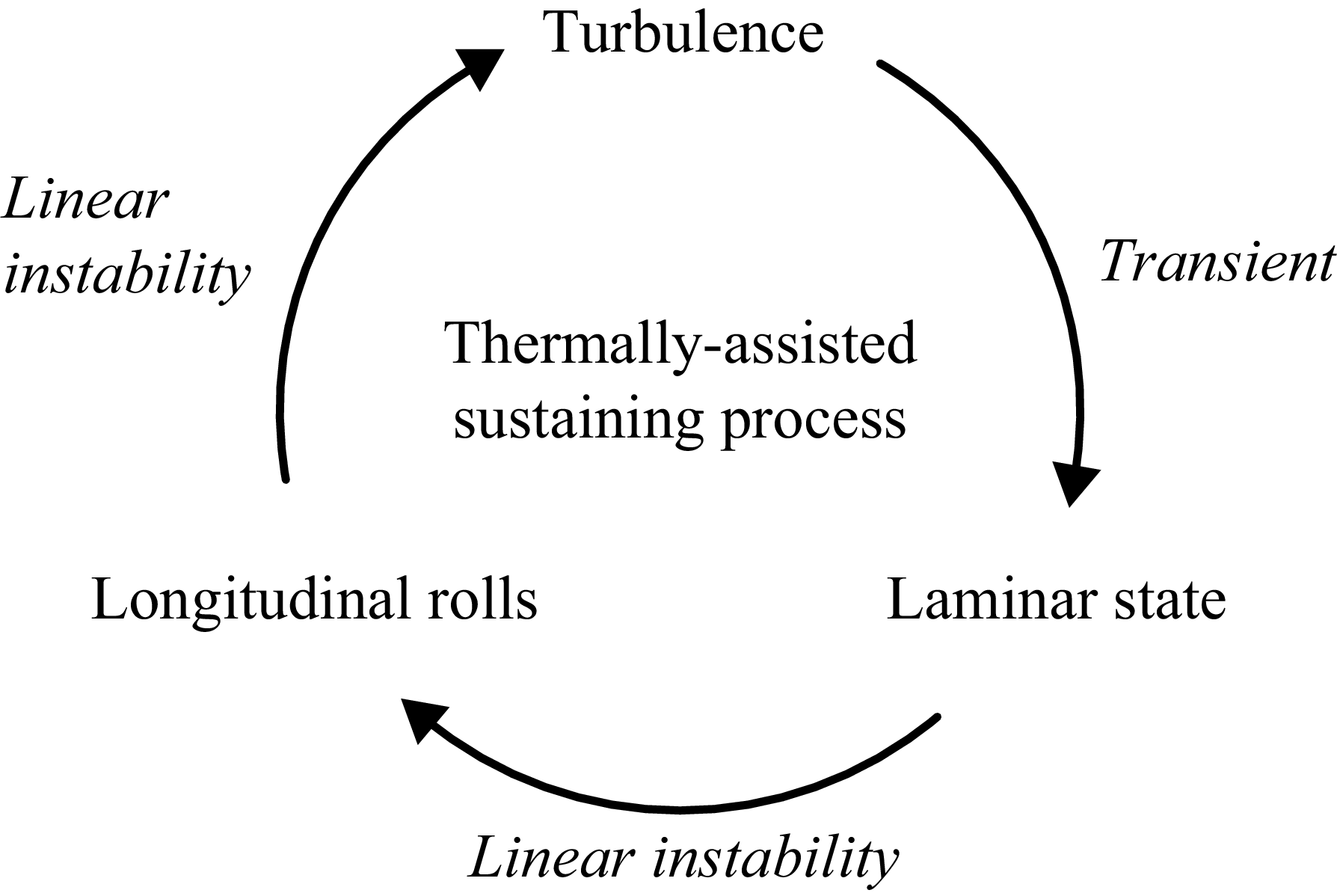


 Open access