


1. Introduction
Stellarators (Spitzer Reference Spitzer1958) are toroidal nuclear fusion devices that are used to study magnetic confinement fusion. Unlike axisymmetric tokamaks, stellarators possess discrete toroidal symmetry. The lack of continuous toroidal symmetry offers considerably greater design freedom, at the expense of trapped particle confinement, a quality guaranteed in axisymmetry through Noether’s theorem (Noether Reference Noether1918). Therefore, we seek stellarators with trapped particle confinement, a property known as omnigenity.
Omnigenous magnetic fields ensure zero bounce-averaged radial drift (Hall & McNamara Reference Hall and McNamara1975; Cary & Shasharina Reference Cary and Shasharina1997), of which both axisymmetry and quasisymmetry are subsets (Boozer Reference Boozer1983; Nührenberg & Zille Reference Nührenberg and Zille1988; Dudt et al. Reference Dudt, Goodman, Conlin, Panici and Kolemen2024). Recent advances in stellarator optimisation have generated omnigenous configurations with excellent neoclassical confinement levels (Landreman & Paul Reference Landreman and Paul2022; Goodman et al. Reference Goodman, Mata, Plunk, Smith, Mackenbach, Beidler and Helander2023). However, these configurations are typically only calculated up to the last closed flux surface (LCFS). To develop a stellarator fusion power plant, it is essential to also predict and optimise the magnetic field structure outside the LCFS (Parra Diaz et al. Reference Parra Diaz2024). This is necessary to separate the high-temperature plasma from the plasma-facing components while efficiently disposing of fusion by-products like helium ash and impurities such as heavier ions.
The structure outside the plasma boundary depends on the boundary shape, so changing the boundary shape is a potential way to obtain a desirable fieldline structure in the edge. Indeed, divertors (Burnett et al. Reference Burnett, Grove, Stix and Wakefield1958) have been greatly successful in tokamaks and offer significantly improved performance over limiters (Wagner et al. Reference Wagner, Becker, Behringer, Campbell, Eberhagen, Engelhardt, Fussmann, Gehre, Gernhardt and Gierke1982). Depending on the boundary shape and coil positions, one can design various divertor configurations in tokamaks such as the single-null, double-null, snowflake (Ryutov Reference Ryutov2007) and super-X (Valanju et al. Reference Valanju, Kotschenreuther, Mahajan and Canik2009). These configurations utilise poloidal and divertor coils to create and shift an X-point – a region in tokamaks where the poloidal field disappears.
Stellarators have utilised three distinct divertor configurations (Bader et al. Reference Bader, Effenberg and Hegna2018a ): helical, resonant and non-resonant divertors. Helical divertors were used in heliotron/torsatron concepts such as the Heliac device (Harris et al. Reference Harris, Cantrell, Hender, Carreras and Morris1985) and LHD (Ohyabu et al. Reference Ohyabu1992). These divertors work by creating a stochastic region with edge surface layers and X-points, which the magnetic fieldlines cross before reaching the scrape-off layer. The coil design and magnetic configuration in the edge surface layers are complex and difficult to predict (Ohyabu et al. Reference Ohyabu1994). Moreover, applicability of this concept to omnigenous stellarators with non-helical symmetry still remains uncertain (Bader et al. Reference Bader, Effenberg and Hegna2018a ), posing challenges for their design and optimisation.
Resonant divertors, used in W7-AS (Grigull et al. Reference Grigull2001; Feng et al. Reference Feng, Sardei, Grigull, McCormick, Kisslinger, Reiter and Igitkhanov2002) and W7-X (Pedersen et al. Reference Pedersen2019), work by leveraging island formation and placing divertors between the X- and O-points of the islands. The island structure depends on the pitch of the fieldline in the boundary, whereas the connection length depends directly on the number of X-points and inversely on the magnetic fieldline pitch and the magnetic shear (Feng et al. Reference Feng, Kobayashi, Lunt and Reiter2011) making them useful for low-magnetic-shear stellarators.
Non-resonant divertors use a more complicated design to create a stochastic field in the edge, but similar to resonant divertors, they can be used to spread the heat load and improve plasma exhaust rejection. These divertors are also more resilient to changes in the magnetic field structure (Bader et al. Reference Bader, Boozer, Hegna, Lazerson and Schmitt2017), but the magnetic field structure in the chaotic field region is complicated to calculate and requires further understanding. Recent work (Boozer & Punjabi Reference Boozer and Punjabi2018; Punjabi & Boozer Reference Punjabi and Boozer2022; Garcia et al. Reference Garcia, Bader, Frerichs, Hartwell, Schmitt, Allen and Schmitz2023; Davies et al. Reference Davies, Smiet, Punjabi, Boozer and Henneberg2025) has further explored the possibility of using non-resonant divertors in stellarators.
Motivated by the need to understand how boundary shaping affects fieldline structure in the edge and X-point and island divertor design, in this paper, we study the umbilic stellarator (US) as a method of achieving control over the edge magnetic field topology, and generate USs for vacuum and finite-
 $\beta$
cases.Footnote
1
Umbilic stellarators are characterised by regions of high curvature on the boundary and how these high-curvature regions are positioned. We develop a technique that allows us to obtain USs by simultaneously optimising a curve and the plasma boundary, and imposing a high curvature along this curve which creates a ridge along the plasma boundary. Additionally, we ensure that all equilibria have reasonable omnigenity, ensuring low neoclassical transport. Finally, we propose an experiment to modify an existing tokamak to a stellarator using our optimisation process and build it using umbilic coils, which are helically wound coils, similar to divertor coils, with fractional helicity that carry a small current (compared with the plasma current), and follow an umbilic edge on the plasma boundary. We show how an umbilic coil can create a high-curvature umbilic region in finite-pressure equilibria, acting as an alternative to modular coils, to create a ridge on the plasma boundary.
$\beta$
cases.Footnote
1
Umbilic stellarators are characterised by regions of high curvature on the boundary and how these high-curvature regions are positioned. We develop a technique that allows us to obtain USs by simultaneously optimising a curve and the plasma boundary, and imposing a high curvature along this curve which creates a ridge along the plasma boundary. Additionally, we ensure that all equilibria have reasonable omnigenity, ensuring low neoclassical transport. Finally, we propose an experiment to modify an existing tokamak to a stellarator using our optimisation process and build it using umbilic coils, which are helically wound coils, similar to divertor coils, with fractional helicity that carry a small current (compared with the plasma current), and follow an umbilic edge on the plasma boundary. We show how an umbilic coil can create a high-curvature umbilic region in finite-pressure equilibria, acting as an alternative to modular coils, to create a ridge on the plasma boundary.
In § 2, we explain the ideal magnetohydrodynamic (MHD) equilibrium. In § 3, we introduce the umbilic boundary shape, how to parametrise them and how we approximate them with DESC, and how to solve the ideal MHD equations throughout the volume enclosed by the approximated shape. In § 4, we present a set of optimised vacuum (
 $\beta = 0$
) and finite-
$\beta = 0$
) and finite-
 $\beta$
stellarators and analyse their properties such as omnigenity. To understand the magnetic field structure in the edge, we design modular coils for the vacuum equilibrium and trace the fieldlines throughout the volume. In order to assess the robustness of the edge magnetic field configuration, we introduce a dummy current source at the magnetic axis to emulate a plasma fluctuation. In § 5, we take the Columbia High-Beta Torus-Extended Pulse (HBT-EP) plasma shape and modify it into an US without changing the coilset used for the original tokamak, just by adding an umbilic coil. We study cases where the umbilic coil carries current in the same (co-
$\beta$
stellarators and analyse their properties such as omnigenity. To understand the magnetic field structure in the edge, we design modular coils for the vacuum equilibrium and trace the fieldlines throughout the volume. In order to assess the robustness of the edge magnetic field configuration, we introduce a dummy current source at the magnetic axis to emulate a plasma fluctuation. In § 5, we take the Columbia High-Beta Torus-Extended Pulse (HBT-EP) plasma shape and modify it into an US without changing the coilset used for the original tokamak, just by adding an umbilic coil. We study cases where the umbilic coil carries current in the same (co-
 $I$
) and opposite (counter-
$I$
) and opposite (counter-
 $I$
) direction as the plasma current
$I$
) direction as the plasma current
 $I$
, study the effect of the umbilic current on edge iota and solve a single-stage problem for the co-
$I$
, study the effect of the umbilic current on edge iota and solve a single-stage problem for the co-
 $I$
case, by simultaneously modifying the plasma boundary and umbilic coil shape. In § 6, we conclude our study by highlighting existing limitations and exploring potential avenues for overcoming them.
$I$
case, by simultaneously modifying the plasma boundary and umbilic coil shape. In § 6, we conclude our study by highlighting existing limitations and exploring potential avenues for overcoming them.
2. Ideal MHD equilibrium
In this section, we briefly explain how we define and calculate an ideal MHD equilibrium in a stellarator. We then explain how to locally vary the gradients of that equilibrium.
A divergence-free magnetic field
 $\boldsymbol{B}$
can be written in the Clebsch form (D’haeseleer et al. Reference D’haeseleer, Hitchon, Callen and Shohet2012):
$\boldsymbol{B}$
can be written in the Clebsch form (D’haeseleer et al. Reference D’haeseleer, Hitchon, Callen and Shohet2012):
 \begin{equation} \boldsymbol{B} = \boldsymbol{\nabla }\psi \times \boldsymbol{\nabla }\alpha . \end{equation}
We focus on solutions whose magnetic fieldlines lie on closed nested toroidal surfaces, known as flux surfaces. We label these surfaces using the enclosed toroidal flux
 $\psi$
. On each flux surface, the lines of constant
$\psi$
. On each flux surface, the lines of constant
 $\alpha$
coincide with the magnetic fieldlines. Thus,
$\alpha$
coincide with the magnetic fieldlines. Thus,
 $\alpha$
is known as the fieldline label. We define
$\alpha$
is known as the fieldline label. We define
 $\alpha = \theta _{\textrm {PEST}} - \iota \zeta$
, where
$\alpha = \theta _{\textrm {PEST}} - \iota \zeta$
, where
 $\theta _{\textrm {PEST}}$
is the
$\theta _{\textrm {PEST}}$
is the
 $\mathrm{PEST}$
straight fieldline angle,
$\mathrm{PEST}$
straight fieldline angle,
 $\zeta$
is the cylindrical toroidal angle and
$\zeta$
is the cylindrical toroidal angle and
 \begin{equation} \iota = \frac {\boldsymbol{B}\boldsymbol{\cdot }\boldsymbol{\nabla }\theta _{\textrm {PEST}}}{\boldsymbol{B}\boldsymbol{\cdot }\boldsymbol{\nabla }\zeta } \end{equation}
is the pitch of the magnetic fieldlines on a flux surface, known as the rotational transform. Using the Clebsch form of the magnetic field, we solve the ideal MHD force balance equation:
 \begin{equation} \boldsymbol{j} \times \boldsymbol{B} = \boldsymbol{\nabla } p, \end{equation}
where the plasma current
 $\boldsymbol{j} = (\boldsymbol{\nabla } \times \boldsymbol{B})/\mu _0$
from Ampere’s law,
$\boldsymbol{j} = (\boldsymbol{\nabla } \times \boldsymbol{B})/\mu _0$
from Ampere’s law,
 $p$
is the plasma pressure and
$p$
is the plasma pressure and
 $\mu _0$
is the vacuum magnetic permeability. Unlike an axisymmetric case, for stellarators we have to solve (2.3) as an optimisation problem. We achieve this with the
$\mu _0$
is the vacuum magnetic permeability. Unlike an axisymmetric case, for stellarators we have to solve (2.3) as an optimisation problem. We achieve this with the
 $\texttt {DESC}$
(Dudt & Kolemen Reference Dudt and Kolemen2020; Conlin et al. Reference Conlin, Dudt, Panici and Kolemen2023; Dudt et al. Reference Dudt, Conlin, Panici and Kolemen2023; Panici et al. Reference Panici, Conlin, Dudt, Unalmis and Kolemen2023) stellarator optimisation suite through minimisation of
$\texttt {DESC}$
(Dudt & Kolemen Reference Dudt and Kolemen2020; Conlin et al. Reference Conlin, Dudt, Panici and Kolemen2023; Dudt et al. Reference Dudt, Conlin, Panici and Kolemen2023; Panici et al. Reference Panici, Conlin, Dudt, Unalmis and Kolemen2023) stellarator optimisation suite through minimisation of
 $F \equiv \boldsymbol{j} \times \boldsymbol{B} - \boldsymbol{\nabla } p$
.
$F \equiv \boldsymbol{j} \times \boldsymbol{B} - \boldsymbol{\nabla } p$
.
 $\texttt {DESC}$
can simultaneously solve an equilibrium while optimising for multiple objectives such as MHD stability, quasisymmetry and more, without re-solving the equilibrium force balance equation (2.3) for each optimisation variable. To reduce the computational cost further, we also use the fact that stellarators possess a discrete toroidal symmetry such that every stellarator comprises several identical sections. The number of identical sections is denoted by the field period
$\texttt {DESC}$
can simultaneously solve an equilibrium while optimising for multiple objectives such as MHD stability, quasisymmetry and more, without re-solving the equilibrium force balance equation (2.3) for each optimisation variable. To reduce the computational cost further, we also use the fact that stellarators possess a discrete toroidal symmetry such that every stellarator comprises several identical sections. The number of identical sections is denoted by the field period
 $n_{\textrm {FP}}$
. Therefore, the force balance problem is only solved in a single field period. In the following sections, we utilise DESC to optimise for omnigenous USs.
$n_{\textrm {FP}}$
. Therefore, the force balance problem is only solved in a single field period. In the following sections, we utilise DESC to optimise for omnigenous USs.
3. Umbilic stellarators
Umbilic stellarators draw inspiration from an umbilic bracelet (or torus) (Zeeman Reference Zeeman1976), a three-dimensional shape with a cross-section that is a deltoid curve, a three-cusped hypocycloid which rotates by
 $\Delta \theta = 2\pi /3$
poloidally after a single toroidal turn
$\Delta \theta = 2\pi /3$
poloidally after a single toroidal turn
 $\Delta \zeta = 2\pi$
. The sharp edge lies exactly on the cusp. Therefore, the sharp edge has to go around three times toroidally before meeting itself. A stellarator generated using an umbilic boundary is potentially advantageous for divertor designs, offering a continuous divertor option with a long connection length. For a smooth magnetic field, the sharp edge of such a boundary would be impossible for a magnetic fieldline. Therefore, the fieldline pitch on the boundary matches the umbilic topology. That is,
$\Delta \zeta = 2\pi$
. The sharp edge lies exactly on the cusp. Therefore, the sharp edge has to go around three times toroidally before meeting itself. A stellarator generated using an umbilic boundary is potentially advantageous for divertor designs, offering a continuous divertor option with a long connection length. For a smooth magnetic field, the sharp edge of such a boundary would be impossible for a magnetic fieldline. Therefore, the fieldline pitch on the boundary matches the umbilic topology. That is,
 $\iota = n_{\textrm {FP}} m/n = 1/3$
, where
$\iota = n_{\textrm {FP}} m/n = 1/3$
, where
 $m, n \in \mathbb{Z}$
corresponding to the poloidal and toroidal motion of the fieldline and
$m, n \in \mathbb{Z}$
corresponding to the poloidal and toroidal motion of the fieldline and
 $n_{\textrm {FP}}$
, the field period, is the measure of discrete symmetry of the stellarator. For a general umbilic shape,
$n_{\textrm {FP}}$
, the field period, is the measure of discrete symmetry of the stellarator. For a general umbilic shape,
 $m/n$
can attain rational values besides
$m/n$
can attain rational values besides
 $1/3$
. Further details are provided in this section.
$1/3$
. Further details are provided in this section.
3.1. Defining an umbilic surface and edge
The initial shape of a stellarator symmetric umbilic-torus-like surface
 $\partial V$
is parametrised as a rotating polygon-like with convex sides:
$\partial V$
is parametrised as a rotating polygon-like with convex sides:
 \begin{align} R_{\mathrm{US}} & = R_0 + 2\varrho \cos \left (\frac {\pi }{2n}\right ) \cos \bigg(\frac {\theta + \frac {\pi }{n} (2 \lfloor n\theta/2\pi \rfloor + 1)}{2}\nonumber \\&\qquad\qquad\qquad\qquad\qquad + \frac {m n_{\textrm {FP}} \zeta + r_1 \sin (n_{\textrm {FP}} \zeta ) + r_4 \sin (2 n_{\textrm {FP}} \zeta )}{n} \bigg)\nonumber \\ & \quad - \varrho \cos \left (\frac {\pi }{n}\left(2 \Big \lfloor \frac {n \theta }{2\pi } \Big \rfloor + 1\right) + \frac {m n_{\textrm {FP}} \zeta + r_1 \sin (n_{\textrm {FP}} \zeta ) + r_4 \sin (2 n_{\textrm {FP}} \zeta )}{n}\right )\nonumber \\&\quad + r_2 \cos (n_{\textrm {FP}} \zeta ), \end{align}
 \begin{align} Z_{\mathrm{US}} &= 2\varrho \cos \left (\frac {\pi }{2n}\right ) \sin \left (\frac {\theta + \frac {\pi }{n} (2 \lfloor {n \theta }/{2\pi } \rfloor + 1)}{2} + \frac {m n_{\textrm {FP}} \zeta + r_5 \sin (n_{\textrm {FP}} \zeta )}{n} \right )\nonumber \\ & - \varrho \sin \left (\frac {\pi }{n}\left(2 \Big \lfloor \frac {n \theta }{2\pi } \Big \rfloor + 1\right) + \frac {m n_{\textrm {FP}} \zeta + r_5 \sin (n_{\textrm {FP}} \zeta )}{n}\right ) + r_3 \sin ( n_{\textrm {FP}} \zeta ), \end{align}
where the major radius
 $ R_0 = 1$
throughout this paper, unless stated otherwise,
$ R_0 = 1$
throughout this paper, unless stated otherwise,
 $\varrho$
is the minor radius of the umbilic-torus-like surface,
$\varrho$
is the minor radius of the umbilic-torus-like surface,
 $\theta$
is the poloidal angle used in DESC,
$\theta$
is the poloidal angle used in DESC,
 $\zeta$
is the cylindrical toroidal angle and
$\zeta$
is the cylindrical toroidal angle and
 $\lfloor \ldots \rfloor$
is the floor function, defined such that
$\lfloor \ldots \rfloor$
is the floor function, defined such that
 \begin{align} \lfloor x \rfloor = \begin{cases} x, & \text{if } x \in \mathbb{Z} \\ N-1, & \text{if } N-1 \lt x \lt N \text{ and } x \notin \mathbb{Z}, \ N \in \mathbb{Z}. \end{cases} \end{align}
In the surface parametrisation, we also define
 $n$
as the umbilic factor, which defines the number of sides in the analytical parametrisation,
$n$
as the umbilic factor, which defines the number of sides in the analytical parametrisation,
 $m$
is an integer that determines the poloidal motion of the sharp umbilic edge and
$m$
is an integer that determines the poloidal motion of the sharp umbilic edge and
 $n_{\textrm {FP}}$
is the field period. The periodicity of the edge is
$n_{\textrm {FP}}$
is the field period. The periodicity of the edge is
 $n_{\textrm {FP}} (m/n)$
– the edge closes on itself after
$n_{\textrm {FP}} (m/n)$
– the edge closes on itself after
 $n/\gcd (n, n_{\textrm {FP}})$
toroidal turns, where
$n/\gcd (n, n_{\textrm {FP}})$
toroidal turns, where
 $\gcd$
is the greatest common divisor. The parameters
$\gcd$
is the greatest common divisor. The parameters
 $r_1, r_4, r_5$
define the convexity/concavity of a cross-section and how it changes toroidally,
$r_1, r_4, r_5$
define the convexity/concavity of a cross-section and how it changes toroidally,
 $r_4$
determines the magnetic axis torsion and
$r_4$
determines the magnetic axis torsion and
 $r_2$
is another parameter that determines the shape of the axis. The shape of such a boundary, the naming convention we use and periodicity of the edge are illustrated in figure 1.
$r_2$
is another parameter that determines the shape of the axis. The shape of such a boundary, the naming convention we use and periodicity of the edge are illustrated in figure 1.
An umbilic boundary design with
 $n_{\textrm {FP}}=4, n=3, m=2, \varrho = 0.344$
. All the rest of the parameters
$n_{\textrm {FP}}=4, n=3, m=2, \varrho = 0.344$
. All the rest of the parameters
 $r_j=0$
in (3.1) and (3.2). In (a) we show the full shape and in (b) we present a single field period from the parametrisation. A point
$r_j=0$
in (3.1) and (3.2). In (a) we show the full shape and in (b) we present a single field period from the parametrisation. A point
 $p_i \in \{0, 1, 2\}$
corresponding to the sharp edge at each toroidal cross-section connects to
$p_i \in \{0, 1, 2\}$
corresponding to the sharp edge at each toroidal cross-section connects to
 $\mod (p_i+m, 3)$
after a single field period. The sharp edge defined by
$\mod (p_i+m, 3)$
after a single field period. The sharp edge defined by
 $R_{\mathrm{US}}(\theta = 0, \zeta ), Z_{\mathrm{US}}(\theta =0, \zeta )$
meets itself after
$R_{\mathrm{US}}(\theta = 0, \zeta ), Z_{\mathrm{US}}(\theta =0, \zeta )$
meets itself after
 $n = 3$
toroidal turns.
$n = 3$
toroidal turns.

The floor function creates the sharp umbilic edge, while the rest of the parameters grant us enough freedom that we can start with a boundary shape that has good quasisymmetry and allows us to create an umbilic edge with any low-order rational periodicity
 $n_{\textrm {FP}} (m/n)$
. It is also stellarator-symmetric, i.e.
$n_{\textrm {FP}} (m/n)$
. It is also stellarator-symmetric, i.e.
 $R_{\mathrm{US}}(\theta , \zeta ) = R_{\mathrm{US}}(-\theta , -\zeta ), Z_{\mathrm{US}}(\theta , \zeta ) = -Z_{\mathrm{US}}(-\theta , -\zeta )$
.
$R_{\mathrm{US}}(\theta , \zeta ) = R_{\mathrm{US}}(-\theta , -\zeta ), Z_{\mathrm{US}}(\theta , \zeta ) = -Z_{\mathrm{US}}(-\theta , -\zeta )$
.
We also define a separate grid on the boundary
 $\rho = 1$
, the umbilic edge, on which a sharp curvature is imposed, defined by values
$\rho = 1$
, the umbilic edge, on which a sharp curvature is imposed, defined by values
 $(\hat {\theta }, \zeta )$
so that
$(\hat {\theta }, \zeta )$
so that
 \begin{equation} \hat {\theta } = \frac {m n_{\textrm {FP}} \zeta + \sum _{k}^{N_{\mathrm{u}}} a_{k} \sin (n_{\textrm {FP}} \zeta )}{n}, \quad \gcd (m, n) = 1. \end{equation}
For the surface parametrisation,
 $\theta = 0$
corresponds to the umbilic edge – initial
$\theta = 0$
corresponds to the umbilic edge – initial
 $\hat {\theta }$
is calculated along this edge but it can change freely during optimisation as the optimiser varies the coefficients
$\hat {\theta }$
is calculated along this edge but it can change freely during optimisation as the optimiser varies the coefficients
 $a_k$
. Note that
$a_k$
. Note that
 $\theta$
is the DESC poloidal angle throughout this paper, unless stated otherwise.
$\theta$
is the DESC poloidal angle throughout this paper, unless stated otherwise.
However, creating and solving with a perfectly sharp edge is difficult with a fully spectral solver. Therefore, in the next section, we explain how we approximate umbilic boundary shapes with the DESC code.
3.2. Approximating umbilic shapes with DESC
DESC uses a Fourier–Zernike spectral representation to solve the force balance equation in the
 $(\rho , \theta , \zeta )$
coordinate system, where
$(\rho , \theta , \zeta )$
coordinate system, where
 $\rho = \sqrt {\psi /\psi _b},\, \theta = \theta _{\textrm {PEST}} - \varLambda (\rho , \theta , \zeta ), \, \zeta = \phi$
, the cylindrical toroidal angle. The problem is defined in a cylindrical coordinate system
$\rho = \sqrt {\psi /\psi _b},\, \theta = \theta _{\textrm {PEST}} - \varLambda (\rho , \theta , \zeta ), \, \zeta = \phi$
, the cylindrical toroidal angle. The problem is defined in a cylindrical coordinate system
 $(R, \zeta , Z)$
by decomposing it into Fourier–Zernike spectral bases (see Panici et al. Reference Panici, Conlin, Dudt, Unalmis and Kolemen2023 for more details):
$(R, \zeta , Z)$
by decomposing it into Fourier–Zernike spectral bases (see Panici et al. Reference Panici, Conlin, Dudt, Unalmis and Kolemen2023 for more details):
 \begin{equation} R(\rho ,\theta ,\zeta ) = \sum _{m=-M,n=-N,l=0}^{M,N,L} R_{lmn} \mathcal{Z}_l^m (\rho ,\theta ) \hat {F}^n(\zeta ), \end{equation}
 \begin{equation} Z(\rho ,\theta ,\zeta ) = \sum _{m=-M,n=-N,l=0}^{M,N,L} Z_{lmn} \mathcal{Z}_l^m (\rho ,\theta ) \hat {F}^n(\zeta ), \end{equation}
where
 $l,\ m$
and
$l,\ m$
and
 $n$
are the radial, poloidal and toroidal mode numbers, whereas
$n$
are the radial, poloidal and toroidal mode numbers, whereas
 $L,\ M$
and
$L,\ M$
and
 $N$
define the largest values of
$N$
define the largest values of
 $l,\ m$
and
$l,\ m$
and
 $n$
, respectively, and
$n$
, respectively, and
 $\mathcal{Z}, \hat {F}$
are Zernike and Fourier basis functions. These parameters define the resolution of a DESC equilibrium.
$\mathcal{Z}, \hat {F}$
are Zernike and Fourier basis functions. These parameters define the resolution of a DESC equilibrium.
To solve the ideal MHD equation inside the umbilic shape, we have to first fit the Fourier–Zernike basis at
 $\rho = 1$
to the umbilic boundary, which requires solving a set of linear equations,
$\rho = 1$
to the umbilic boundary, which requires solving a set of linear equations,
 \begin{eqnarray} \left [\begin{array}{cc} \sum _{m=-M,n=-N,l=0}^{M,N,L} R_{lmn} \mathcal{Z}_l^m (\rho = 1,\theta ) \hat {F}^n(\zeta )\\[4pt] \sum _{m=-M,n=-N,l=0}^{M,N,L} Z_{lmn} \mathcal{Z}_l^m (\rho = 1,\theta ) \hat {F}^n(\zeta ) \end{array}\right ] = \left [\begin{array}{cc} R_{\mathrm{US}}(\theta , \zeta )\\[4pt] Z_{\mathrm{US}}(\theta , \zeta ) \end{array}\right ]\!, \end{eqnarray}
to find
 $R_{lmn}, Z_{lmn}$
so that the boundary shape matches with the umbilic parametrisation. Similarly, to obtain
$R_{lmn}, Z_{lmn}$
so that the boundary shape matches with the umbilic parametrisation. Similarly, to obtain
 $a_k$
, we parametrise the umbilic edge using
$a_k$
, we parametrise the umbilic edge using
 $R_{\mathrm{curve}} = R(\rho =1,$
 $\theta =0, \zeta ), Z_{\mathrm{curve}} = Z(\rho = 1, \theta =0, \zeta )$
, and perform an inverse Fourier transform to obtain
$\theta =0, \zeta ), Z_{\mathrm{curve}} = Z(\rho = 1, \theta =0, \zeta )$
, and perform an inverse Fourier transform to obtain
 $a_k$
. Note that upon fitting a spectral basis, the umbilic edge is smoothed out. After representing the umbilic shape in the Fourier–Zernike basis, we solve the ideal MHD equation inside the volume. Figure 2 illustrates this process of fitting and solving force balance in a US131 boundary shape.
$a_k$
. Note that upon fitting a spectral basis, the umbilic edge is smoothed out. After representing the umbilic shape in the Fourier–Zernike basis, we solve the ideal MHD equation inside the volume. Figure 2 illustrates this process of fitting and solving force balance in a US131 boundary shape.
Contour plot of the flux surface average force balance error
 $|F|$
plotted on the cross-section
$|F|$
plotted on the cross-section
 $\zeta = 0$
of a vacuum DESC equilibrium created using a US131 boundary with
$\zeta = 0$
of a vacuum DESC equilibrium created using a US131 boundary with
 $\rho = 0.1,\ r_1=0.133,\ r_5=0.1$
. The actual boundary (in solid black) is obtained after fitting a Fourier–Zernike series to the true umbilic boundary (in dashed blue). The resolution of the DESC equilibrium is
$\rho = 0.1,\ r_1=0.133,\ r_5=0.1$
. The actual boundary (in solid black) is obtained after fitting a Fourier–Zernike series to the true umbilic boundary (in dashed blue). The resolution of the DESC equilibrium is
 $L=M=N=14$
and the resolution of the umbilic curve is
$L=M=N=14$
and the resolution of the umbilic curve is
 $N_{\mathrm{u}} = 12$
.
$N_{\mathrm{u}} = 12$
.

The sharpness of the umbilic edge increases as we increase the resolution of the fit surface and the agreement between
 $\texttt {DESC}$
and the umbilic parametrisation improves. Alternatively, one may use a double-Chebyshev (Fortunato Reference Fortunato2024) instead of a double-Fourier representation to improve the spectral fit, local basis methods such as finite element to represent and solve the equilibrium or use a nonlinear transformation to map the circular torus in the Fourier–Zernike basis to an umbilic shape, similar to the transformation used for circular tokamaks by Webster & Gimblett (Reference Webster and Gimblett2009). However, using a new basis and performing equilibrium optimisation are beyond the scope of this work.
$\texttt {DESC}$
and the umbilic parametrisation improves. Alternatively, one may use a double-Chebyshev (Fortunato Reference Fortunato2024) instead of a double-Fourier representation to improve the spectral fit, local basis methods such as finite element to represent and solve the equilibrium or use a nonlinear transformation to map the circular torus in the Fourier–Zernike basis to an umbilic shape, similar to the transformation used for circular tokamaks by Webster & Gimblett (Reference Webster and Gimblett2009). However, using a new basis and performing equilibrium optimisation are beyond the scope of this work.
In the following section, we discuss how, beginning with the parametrisation of the umbilic surface, we can optimise for omnigenous USs.
3.3. Optimising an umbilic equilibrium with DESC
As we noted in the previous section and figure 2, after fitting a Fourier–Zernike basis to the umbilic boundary, it becomes smooth because approximating a sharp boundary with a double-Fourier representation is usually difficult. Therefore, we have to modify the optimisation process for an umbilic equilibrium to maintain a high curvature, instead of a perfectly sharp umbilic edge. Additionally, for these shapes to be practically feasible fusion reactors, we also need good omnigenity. Therefore, we use the omnigenity and effective ripple objectives to improve the omnigenity throughout the volume.
After fitting to a Fourier–Zernike basis, the high-curvature edge, in general, does not align with the fieldline. In the unoptimised shape defined in (3.1) and (3.2), the
 $\iota$
is typically too small because of weak shaping. Therefore, we have to optimise separately for a boundary rotational transform to be close
$\iota$
is typically too small because of weak shaping. Therefore, we have to optimise separately for a boundary rotational transform to be close
 $n_{\textrm {FP}} m/n$
. Also, to ensure that the umbilic edge curve matches with the fieldline labelled
$n_{\textrm {FP}} m/n$
. Also, to ensure that the umbilic edge curve matches with the fieldline labelled
 $\alpha =0$
, we enforce a strong negative curvature
$\alpha =0$
, we enforce a strong negative curvature
 $\kappa _{2, \rho }$
along the umbilic edge defined by (3.4). The definitions of the principal curvatures are given in Appendix A. The overall objective function is
$\kappa _{2, \rho }$
along the umbilic edge defined by (3.4). The definitions of the principal curvatures are given in Appendix A. The overall objective function is
 \begin{eqnarray} \mathcal{F}_{\text{stage-one}} = w_{A}\, f_{\mathrm{aspect}}^2 + w_{\iota }\, f_{\textrm {iota}}^2 + w_{O}\, f_{\mathrm{om}}^2 + w_{U}\, f_{\mathrm{umbilic}}^2 + w_R\, f_{\mathrm{ripple}}^2, \end{eqnarray}
where
 $f_{x}$
are various objectives on the right-hand side for aspect ratio, boundary rotational transform, omnigenity, high curvature along the umbilic edge and effective ripple and
$f_{x}$
are various objectives on the right-hand side for aspect ratio, boundary rotational transform, omnigenity, high curvature along the umbilic edge and effective ripple and
 $w_A, w_{\iota }, w_{O}, w_{U}, w_{R}$
are weights used with each objective function. The exact definitions of these objectives are provided in Appendix B. At each iteration of a DESC optimisation,
$w_A, w_{\iota }, w_{O}, w_{U}, w_{R}$
are weights used with each objective function. The exact definitions of these objectives are provided in Appendix B. At each iteration of a DESC optimisation,
 $\mathcal{F}_{\text{stage-one}}$
is minimised while satisfying (2.3). Mathematically,
$\mathcal{F}_{\text{stage-one}}$
is minimised while satisfying (2.3). Mathematically,
 \begin{equation} \min \mathcal{F}_{\text{stage-one}}(\hat {\boldsymbol{p}}), \qquad \textrm {s.t.} \quad \boldsymbol{\nabla }\left (\mu _0 p + \frac {B^2}{2}\right ) - \boldsymbol{B}\boldsymbol{\cdot }\boldsymbol{\nabla }\boldsymbol{B} = 0,\quad \psi _{\mathrm{b}} = \psi _{\mathrm{b}0}, \end{equation}
where
 $\psi _{\mathrm{b}0}$
is the user-provided enclosed toroidal flux by the boundary and
$\psi _{\mathrm{b}0}$
is the user-provided enclosed toroidal flux by the boundary and
 $\hat {\boldsymbol{p}} \in \{R_{\mathrm{b}, mn}, Z_{\mathrm{b}, mn}, a_k\}$
comprises parameters that determine the boundary shape and the position of the umbilic curve on the boundary. With the objective
$\hat {\boldsymbol{p}} \in \{R_{\mathrm{b}, mn}, Z_{\mathrm{b}, mn}, a_k\}$
comprises parameters that determine the boundary shape and the position of the umbilic curve on the boundary. With the objective
 $\mathcal{F}_{\text{stage-one}}$
defined, we run DESC on a single NVIDIA A100 GPU. A single optimisation takes less than
$\mathcal{F}_{\text{stage-one}}$
defined, we run DESC on a single NVIDIA A100 GPU. A single optimisation takes less than
 $90$
minutes.
$90$
minutes.
4. Omnigenous umbilic stellarators
In this section, we develop two omnigenous umbilic equilibria using the process explained in the previous sections. The first equilibrium is a single-field-period vacuum stellarator with
 $n=3, m = 1$
umbilic topology for which we also design coils, and the second equilibrium is a two-field-period finite-
$n=3, m = 1$
umbilic topology for which we also design coils, and the second equilibrium is a two-field-period finite-
 $\beta$
stellarator with
$\beta$
stellarator with
 $n=5, m=2$
umbilic topology.
$n=5, m=2$
umbilic topology.
4.1. A US131(
 $n_{\textrm {FP}} = 1, n=3, m =1$
) omnigenous vacuum stellarator
$n_{\textrm {FP}} = 1, n=3, m =1$
) omnigenous vacuum stellarator
We begin by calculating an omnigenous vacuum equilibrium with a single field period
 $n_{\textrm {FP}} = 1$
,
$n_{\textrm {FP}} = 1$
,
 $n=3, m=1$
. To do this, we start with the US131 boundary shape, using the parametrisation from § 3.1 with
$n=3, m=1$
. To do this, we start with the US131 boundary shape, using the parametrisation from § 3.1 with
 ${\varrho }=0.1\, \textrm {m},\ r_1 = 0.133,\ r_5 = 0.1$
and the rest of the parameters
${\varrho }=0.1\, \textrm {m},\ r_1 = 0.133,\ r_5 = 0.1$
and the rest of the parameters
 $r_j = 0$
. The toroidal flux enclosed by the initial equilibrium is
$r_j = 0$
. The toroidal flux enclosed by the initial equilibrium is
 $\psi _{\textrm {b}} = \pi {\varrho }^2\ (\textrm{Tm}^2)$
. This shape is then approximated by DESC as explained in § 3.2 and optimised as described in § 3.3 with
$\psi _{\textrm {b}} = \pi {\varrho }^2\ (\textrm{Tm}^2)$
. This shape is then approximated by DESC as explained in § 3.2 and optimised as described in § 3.3 with
 $w_{\textrm{O}} = 0$
Footnote
2
to obtain an omnigenous equilibrium with an aspect ratio
$w_{\textrm{O}} = 0$
Footnote
2
to obtain an omnigenous equilibrium with an aspect ratio
 $A = 10.5$
. The results are presented in figures 3 and 4.
$A = 10.5$
. The results are presented in figures 3 and 4.
The US131 optimisation results showing a significant increase in magnetic axis torsion in (a) from the initial (dotted) to the optimised (solid) boundary. This leads to an increase in the rotational transform, as shown in (b) such that
 $\iota (\rho = 1)$
approaches
$\iota (\rho = 1)$
approaches
 $1/3$
. The shaping also leads the fieldlines to align with the umbilic edge in the optimised equilibrium as shown in (c).
$1/3$
. The shaping also leads the fieldlines to align with the umbilic edge in the optimised equilibrium as shown in (c).

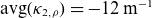
To ensure that the high-curvature umbilic edge is aligned with the magnetic fieldlines, the boundary undergoes deformation, which results in an increased rotational transform. The optimised design minimises the objective
 $\mathcal{F}_{\text{stage-one}}$
while ensuring that the normalised second principal curvature is the lowest along the umbilic edge. The curvature on the umbilic edge is in the range
$\mathcal{F}_{\text{stage-one}}$
while ensuring that the normalised second principal curvature is the lowest along the umbilic edge. The curvature on the umbilic edge is in the range
 $\kappa _{2, \rho } \in [-187, -70]\, {\rm m}^{-1}$
whereas the average curvature on the rest of the boundary is
$\kappa _{2, \rho } \in [-187, -70]\, {\rm m}^{-1}$
whereas the average curvature on the rest of the boundary is
 $\mathrm{avg}(\kappa _{2, \rho }) = -12 \,{\rm m}^{-1}$
. This causes the magnetic fieldline to stay close to the umbilic edge throughout the range
$\mathrm{avg}(\kappa _{2, \rho }) = -12 \,{\rm m}^{-1}$
. This causes the magnetic fieldline to stay close to the umbilic edge throughout the range
 $\zeta \in [0, 6 \pi ]$
as shown in figure 3(c). In the limit where the edge is perfectly sharp, the fieldline will coincide with the umbilic edge.
$\zeta \in [0, 6 \pi ]$
as shown in figure 3(c). In the limit where the edge is perfectly sharp, the fieldline will coincide with the umbilic edge.
The optimised US case is able to achieve an effective ripple
 $\epsilon _{\mathrm{eff}}$
of less than
$\epsilon _{\mathrm{eff}}$
of less than
 $2\,\%$
(
$2\,\%$
(
 $\epsilon _{\mathrm{eff}}^{3/2} \lt 0.0028$
) for most of the volume
$\epsilon _{\mathrm{eff}}^{3/2} \lt 0.0028$
) for most of the volume
 $(\rho \lt 0.86)$
and
$(\rho \lt 0.86)$
and
 $\epsilon _{\mathrm{eff}}^{3/2} \leqslant 0.001$
for
$\epsilon _{\mathrm{eff}}^{3/2} \leqslant 0.001$
for
 $\rho \leqslant 0.6$
. This ensures that neoclassical transport in the
$\rho \leqslant 0.6$
. This ensures that neoclassical transport in the
 $1/\nu$
low-collisionality regime will not deteriorate the device performance in the core but may deteriorate confinement in the edge. An interesting observation is that we can achieve a low ripple transport despite the lack of a specific helicity of the
$1/\nu$
low-collisionality regime will not deteriorate the device performance in the core but may deteriorate confinement in the edge. An interesting observation is that we can achieve a low ripple transport despite the lack of a specific helicity of the
 $B$
contours in the Boozer plot (figure 4
b). This is an instance of a piecewise-omnigenous (Velasco et al. Reference Velasco, Calvo, Escoto, Sánchez, Thienpondt and Parra2024) field that is far from quasisymmetry. Since we did not seek omnigenity with a specific helicity (
$B$
contours in the Boozer plot (figure 4
b). This is an instance of a piecewise-omnigenous (Velasco et al. Reference Velasco, Calvo, Escoto, Sánchez, Thienpondt and Parra2024) field that is far from quasisymmetry. Since we did not seek omnigenity with a specific helicity (
 $w_{\mathrm{O}} = 0$
), the effective ripple penalty acted as a proxy for omnigenity, leading to a piecewise-omnigenous configuration. To prove that these configurations are piecewise-omnigenous, we analyse the normalised second adiabatic invariant
$w_{\mathrm{O}} = 0$
), the effective ripple penalty acted as a proxy for omnigenity, leading to a piecewise-omnigenous configuration. To prove that these configurations are piecewise-omnigenous, we analyse the normalised second adiabatic invariant
 $\tilde {\mathcal{J}}_{\parallel }$
in Appendix C.
$\tilde {\mathcal{J}}_{\parallel }$
in Appendix C.
Output from the vacuum US131 optimisation showing Boozer plots on the boundary and the effective ripple. The output in (b) does not have a specific helicity but still achieves a low ripple transport.

For a vacuum problem, obtaining the right fieldline pitch (
 $\iota = n_{\textrm {FP}} m/n$
) on the boundary and ensuring force balance over a perfectly sharp (unapproximated) boundary make this problem difficult to solve compared with a finite-
$\iota = n_{\textrm {FP}} m/n$
) on the boundary and ensuring force balance over a perfectly sharp (unapproximated) boundary make this problem difficult to solve compared with a finite-
 $\beta$
equilibrium where one can specify the fieldline pitch throughout the volume. Therefore, we have compromised by creating a high-curvature edge instead of a perfectly sharp edge (
$\beta$
equilibrium where one can specify the fieldline pitch throughout the volume. Therefore, we have compromised by creating a high-curvature edge instead of a perfectly sharp edge (
 $\kappa _{2, \rho } \rightarrow \infty$
). If one were to use an alternative representation to represent a perfectly sharp boundary and solve this problem exactly, we would observe the rotational transform almost identical to the initial equilibrium in figure 4(c) sharply rising to
$\kappa _{2, \rho } \rightarrow \infty$
). If one were to use an alternative representation to represent a perfectly sharp boundary and solve this problem exactly, we would observe the rotational transform almost identical to the initial equilibrium in figure 4(c) sharply rising to
 $\iota = m\, n_{\textrm {FP}}/n$
at the edge.The behaviour of high-shear regions near sharp points would be similar to what is observed in tokamaks.
$\iota = m\, n_{\textrm {FP}}/n$
at the edge.The behaviour of high-shear regions near sharp points would be similar to what is observed in tokamaks.
4.2. Modular coil design for the US131 equilibrium
In this section, we design modular coils for the US131 case using the DESC optimiser and elucidate the various difficulties faced when designing modular coils for strongly shaped USs. We create a coilset of
 $32$
(stellarator-symmetric with
$32$
(stellarator-symmetric with
 $16$
unique coils) coils using the Python implementation of REGCOIL (Landreman Reference Landreman2017; Panici et al. Reference Panici2025) in DESC. Starting with this initial coilset, we then perform stage-two optimisation, where we fix the equilibrium boundary and allow the shape of the modular coils to change while minimising the objective
$16$
unique coils) coils using the Python implementation of REGCOIL (Landreman Reference Landreman2017; Panici et al. Reference Panici2025) in DESC. Starting with this initial coilset, we then perform stage-two optimisation, where we fix the equilibrium boundary and allow the shape of the modular coils to change while minimising the objective
 \begin{eqnarray} \mathcal{F}_{\textrm {stage-two}} = (B_{\textrm {out}}^2 - (B_{\textrm {in}}^2 + 2 \mu _0 p))^2 + (\boldsymbol{B}_{\textrm {out}} \boldsymbol{\cdot }\boldsymbol{\hat {n}})^2 \end{eqnarray}
on the plasma boundary. Note that in stage-two optimisation, we ignore the surface current
 $\boldsymbol{K} = (\boldsymbol{B}_{\textrm {out}} - \boldsymbol{B}_{\textrm {in}}) \times \boldsymbol{\hat {n}}$
. Therefore, to verify our solution, we calculate the fieldline trajectory due to the coils and create a Poincaré plot. The original fixed-boundary solution, its comparison with the Poincaré cross-section and the optimised coilset are presented in figure 5.
$\boldsymbol{K} = (\boldsymbol{B}_{\textrm {out}} - \boldsymbol{B}_{\textrm {in}}) \times \boldsymbol{\hat {n}}$
. Therefore, to verify our solution, we calculate the fieldline trajectory due to the coils and create a Poincaré plot. The original fixed-boundary solution, its comparison with the Poincaré cross-section and the optimised coilset are presented in figure 5.
Coils and
 $\boldsymbol{B}_{\mathrm{out}}\boldsymbol{\cdot }\hat {\boldsymbol{n}}$
error plotted on the plasma boundary. Here
$\boldsymbol{B}_{\mathrm{out}}\boldsymbol{\cdot }\hat {\boldsymbol{n}}$
error plotted on the plasma boundary. Here
 $\mathrm{max}|(\boldsymbol{B}_{\mathrm{out}}\boldsymbol{\cdot }\hat {\boldsymbol{n}})/\boldsymbol{B}_{\mathrm{out}}| \leqslant 1\,\%$
. Only one group of unique coils are plotted. At the upper right we plot the Poincaré cross-section at
$\mathrm{max}|(\boldsymbol{B}_{\mathrm{out}}\boldsymbol{\cdot }\hat {\boldsymbol{n}})/\boldsymbol{B}_{\mathrm{out}}| \leqslant 1\,\%$
. Only one group of unique coils are plotted. At the upper right we plot the Poincaré cross-section at
 $\zeta =0$
along with the fixed-boundary solution (in red). The grey curves mark a favourable position to place a divertor. At the lower right we plot the
$\zeta =0$
along with the fixed-boundary solution (in red). The grey curves mark a favourable position to place a divertor. At the lower right we plot the
 $\boldsymbol{B}_{\mathrm{out}}\boldsymbol{\cdot }\hat {\boldsymbol{n}}$
error on a two-dimensional plane along with the umbilic edge (dashed purple).
$\boldsymbol{B}_{\mathrm{out}}\boldsymbol{\cdot }\hat {\boldsymbol{n}}$
error on a two-dimensional plane along with the umbilic edge (dashed purple).

Note that even though the curvature along the umbilic ridge is high, it does not behave like a perfect X-point (or X-line) as the fieldline structure becomes chaotic in the edge and resembles the ‘turnstiles’ topology discussed by Punjabi & Boozer (Reference Punjabi and Boozer2022). However, even though the fieldlines do not exit in the regions of the highest curvature, like a tokamak X-point, the Poincaré traces of the fieldlines stay aligned with the plasma boundary and ‘flare’ near the umbilic edge, which still makes the umbilic edge a favourable location to place divertors or limiters. This study indicates that the behaviour of magnetic fieldlines for a high-curvature ridge can differ significantly from that for a perfectly sharp edge.
Another observation is that modular coil design becomes complicated for umbilic equilibria as seen in the figure. The coils assume high curvature to reduce the normal field error along the umbilic edge. Increasing the number of coils improves the agreement of the fixed-boundary solution with the Poincaré cross-section and reduces the maximum coil curvature but also reduces the coil–coil distance. However, the number of modular coils needed for these umbilic equilibria already exceeds the number of coils used for a single field period for a typical stellarator, which is almost always less than 10.
Finally, we note that the regions of maximum normal field error are parallel to the umbilic edge so that, on average,
 $\boldsymbol{b} \boldsymbol{\cdot }\boldsymbol{\nabla } (\boldsymbol{B}_{\mathrm{out}}\boldsymbol{\cdot }\hat {\boldsymbol{n}}) = 0$
.Footnote
3
This pattern indicates a hidden relationship between the normal field error and the second principal curvature in USs.
$\boldsymbol{b} \boldsymbol{\cdot }\boldsymbol{\nabla } (\boldsymbol{B}_{\mathrm{out}}\boldsymbol{\cdot }\hat {\boldsymbol{n}}) = 0$
.Footnote
3
This pattern indicates a hidden relationship between the normal field error and the second principal curvature in USs.
To ensure practical coil design for USs, a better technique would be to perform single-stage optimisation, which simultaneously changes the plasma boundary and coil shapes, a union of
 $\mathcal{F}_{\text{stage-one}}$
and
$\mathcal{F}_{\text{stage-one}}$
and
 $\mathcal{F}_{\text{stage-two}}$
, accounting for the coil complexity while maintaining omnigenity inside the plasma volume. This is done in § 5.2 for a simpler problem. Another possibility is to use umbilic coils, helically wound divertor-like coils with a fractional helicity (
$\mathcal{F}_{\text{stage-two}}$
, accounting for the coil complexity while maintaining omnigenity inside the plasma volume. This is done in § 5.2 for a simpler problem. Another possibility is to use umbilic coils, helically wound divertor-like coils with a fractional helicity (
 $m/n$
) that carry a small current that pushes (pulls) the plasma away from (towards) itself, creating cusp-like regions, leading to a high-curvature umbilic edge. We do a similar optimisation to modify a tokamak in § 5.1, where we add an umbilic coil without changing the shape of the toroidal field coils to create an umbilic edge. In the next section, we use the same optimisation process to create a finite-
$m/n$
) that carry a small current that pushes (pulls) the plasma away from (towards) itself, creating cusp-like regions, leading to a high-curvature umbilic edge. We do a similar optimisation to modify a tokamak in § 5.1, where we add an umbilic coil without changing the shape of the toroidal field coils to create an umbilic edge. In the next section, we use the same optimisation process to create a finite-
 $\beta$
, omnigenous US.
$\beta$
, omnigenous US.
4.3. A US131 sensitivity analysis of the field structure in the edge
In this section, we introduce a line current source along the magnetic axis of the US131 configuration. The line current aims to simulate an internal fluctuation within the plasma. For different values of the current source strength, we perform the fieldline integration across the entire volume. The purpose of this investigation is to assess the resilience of the fieldline structure at the edge of the US131 stellarator and to determine the extent of modification required for the divertor configuration. We present the fieldline structure for different values of the current in figure 6.
Poincare plots at
 $\zeta = 0$
with a current source placed on-axis for different values of the current, compared with the original fixed-boundary solution (in red). Increasing the current significantly reduces the nestedness of the flux surfaces but the fieldline structure in the edge still ‘flares’ out near the high-curvature edges and the divertor placement does not need to be modified.
$\zeta = 0$
with a current source placed on-axis for different values of the current, compared with the original fixed-boundary solution (in red). Increasing the current significantly reduces the nestedness of the flux surfaces but the fieldline structure in the edge still ‘flares’ out near the high-curvature edges and the divertor placement does not need to be modified.

We observe that even though the flux surfaces inside the plasma boundary lose nestedness and become stochastic, the divertor structure used for the unperturbed US131 case is still an effective choice for this equilibrium, i.e. the fieldline structure in the edge is resilient to fluctuations inside the plasma. Another observation is the emergence of ‘O’-point-like structures near the high-curvature regions in figure 6(b).
4.4. A US252
$(n_{\textrm {FP}}=2, n=5, m=2)$
omnigenous finite-
$\beta$
stellarator


In this section, we generate a two-field-period
 $n=5, m = 2$
finite-
$n=5, m = 2$
finite-
 $\beta$
stellarator. We start with the umbilic parametrisation defined in § 3.1 with
$\beta$
stellarator. We start with the umbilic parametrisation defined in § 3.1 with
 $\varrho =0.1,\ r_1 = 0.133,\ r_5 = 0.1$
and use a pressure profile
$\varrho =0.1,\ r_1 = 0.133,\ r_5 = 0.1$
and use a pressure profile
 $p = 5 \times 10^3 (1-\rho ^2)\, \mathrm{Pa}$
, a rotational transform
$p = 5 \times 10^3 (1-\rho ^2)\, \mathrm{Pa}$
, a rotational transform
 $\iota = 0.755 + 0.043 \rho ^2$
and an enclosed toroidal flux
$\iota = 0.755 + 0.043 \rho ^2$
and an enclosed toroidal flux
 $\psi _{\textrm {b}} = \pi {\varrho }^2 = 0.00314\, \textrm {T m}^2$
. This creates an equilibrium with
$\psi _{\textrm {b}} = \pi {\varrho }^2 = 0.00314\, \textrm {T m}^2$
. This creates an equilibrium with
 $\beta = 0.5\,\%$
.
$\beta = 0.5\,\%$
.
A finite-
 $\beta$
stellarator provides more freedom compared with a vacuum case because the rotational transform can come from a combination of boundary shaping and plasma current. Therefore, we can achieve a higher rotational transform and use the additional freedom to achieve a much lower ripple transport compared with the vacuum case presented in the previous section. The optimisation uses the same objective function defined in (3.8) with the pressure and iota profiles fixed and
$\beta$
stellarator provides more freedom compared with a vacuum case because the rotational transform can come from a combination of boundary shaping and plasma current. Therefore, we can achieve a higher rotational transform and use the additional freedom to achieve a much lower ripple transport compared with the vacuum case presented in the previous section. The optimisation uses the same objective function defined in (3.8) with the pressure and iota profiles fixed and
 $w_{\iota } = 0$
. These results are presented in figure 7.
$w_{\iota } = 0$
. These results are presented in figure 7.
Optimisation output showing the (a) initial and (b) final magnetic field strength Boozer plots and (c) the effective ripple. The black lines in (a) correspond to the magnetic fieldlines and the dashed lines correspond to the umbilic curve. The optimised configuration is another instance of piecewise omnigenity.

We can see in figure 7 that the ridges in the Boozer plots are only clearly visible in the initial equilibrium, which is close to quasisymmetry. The magnetic field of the optimised omnigenous equilibrium does not have any visible ridges in the Boozer plot, even though the curvature along the umbilic ridge increases after optimisation. This indicates that the appearance of ridges in the Boozer representation may only be a feature of quasisymmetric stellarators.
This equilibrium is optimised for poloidal omnigenity but, due to the umbilic curvature penalty, limits the poloidal omnigenity to the low-field region. The Boozer plot in figure 7(b) looks qualitatively like a piecewise-omnigenous Velasco et al. (Reference Velasco, Calvo, Escoto, Sánchez, Thienpondt and Parra2024) configuration, which looks similar to the magnetic field in the W7-X stellarator. The piecewise omnigenity of this equilibrium is demonstrated further in Appendix C. We also plot the cross-section of the equilibrium along with the second principal curvature in figure 8. The neoclassical transport coefficient
 $\epsilon _{\mathrm{eff}}^{3/2} \lt 0.001$
for most (
$\epsilon _{\mathrm{eff}}^{3/2} \lt 0.001$
for most (
 $\rho \lt 0.7$
) of the volume, which means the equilibrium is omnigenous in the core.
$\rho \lt 0.7$
) of the volume, which means the equilibrium is omnigenous in the core.
Cross-section and three-dimensional shape of the optimised US252 equilibrium. The aspect ratio of the optimised equilibrium is
 $A = 6.5$
. In (c), we see that around half of the rotational transform of the optimised equilibrium comes from shaping (Hirshman & Hogan Reference Hirshman and Hogan1986) reducing the dependence on external current drive.
$A = 6.5$
. In (c), we see that around half of the rotational transform of the optimised equilibrium comes from shaping (Hirshman & Hogan Reference Hirshman and Hogan1986) reducing the dependence on external current drive.

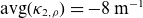
We also observe that the optimised equilibrium deforms and rotates as we move toroidally, while maintaining high curvature along the umbilic curve. The curvature along the umbilic edge
 $\kappa _{2, \rho } \in [-67, -36]\, {\rm m}^{-1}$
while the average curvature on the rest of the plasma boundary is
$\kappa _{2, \rho } \in [-67, -36]\, {\rm m}^{-1}$
while the average curvature on the rest of the plasma boundary is
 $\mathrm{avg} (\kappa _{2, \rho }) = -8\, {\rm m}^{-1}$
. The variation in the curvature is broad, indicating that imposing high curvature at specific locations may be more suitable than others. This can be readily accomplished by selecting sections of the umbilic curve where high curvature is applied and could be a potential way to place potential locations for non-resonant divertors (Bader et al. Reference Bader, Hegna, Cianciosa and Hartwell2018b
).
$\mathrm{avg} (\kappa _{2, \rho }) = -8\, {\rm m}^{-1}$
. The variation in the curvature is broad, indicating that imposing high curvature at specific locations may be more suitable than others. This can be readily accomplished by selecting sections of the umbilic curve where high curvature is applied and could be a potential way to place potential locations for non-resonant divertors (Bader et al. Reference Bader, Hegna, Cianciosa and Hartwell2018b
).
5. Umbilic coil design for a finite-
$\beta$
equilibrium

As we have seen in § 4.1, creating modular coils for vacuum umbilic equilibria is a difficult task due to the sharp curvature regions. Therefore, in this section, we present an alternative strategy that uses umbilic coils to create a US111 finite-
 $\beta$
equilibrium. Instead of modifying modular coils, we use an umbilic coil, a low-current, helically wound coil, similar to a divertor coil in tokamaks, which can be used to create an umbilic edge. Unlike tokamak divertor coils, an umbilic coil is non-axisymmetric and can have a fractional helicity. In the following sections, we discuss two cases, categorised by the direction of the current in the umbilic coils with respect to the toroidal plasma current.
$\beta$
equilibrium. Instead of modifying modular coils, we use an umbilic coil, a low-current, helically wound coil, similar to a divertor coil in tokamaks, which can be used to create an umbilic edge. Unlike tokamak divertor coils, an umbilic coil is non-axisymmetric and can have a fractional helicity. In the following sections, we discuss two cases, categorised by the direction of the current in the umbilic coils with respect to the toroidal plasma current.
5.1. A US111 with an umbilic coil current opposite to the plasma current (counter-
$I$
case)

Umbilic coils differ from helical coils by creating a ridge that may serve as a potential location for an X-point. These coils are similar to tokamak divertor coils, albeit without axisymmetry. To demonstrate their applicability, we modify an
 $n=1$
MHD-stable equilibrium from the HBT-EP experiment (
$n=1$
MHD-stable equilibrium from the HBT-EP experiment (
 $R_0 = 0.94\, {\rm m},\ A = 7.5$
) by adding an
$R_0 = 0.94\, {\rm m},\ A = 7.5$
) by adding an
 $m = 1, n = 1$
ridge to it, breaking its axisymmetry, and then design an umbilic coil for it without modifying the toroidal or vertical field coils. The specific details of the equilibrium used are given in Appendix D.
$m = 1, n = 1$
ridge to it, breaking its axisymmetry, and then design an umbilic coil for it without modifying the toroidal or vertical field coils. The specific details of the equilibrium used are given in Appendix D.
To accomplish this, we start by using
 $20$
toroidal field (TF)Footnote
4
coils and
$20$
toroidal field (TF)Footnote
4
coils and
 $4$
vertical field poloidal (PF) coils as done in the original HBT-EP experiment (Gates Reference Gates1993; Sankar et al. Reference Sankar1993) and add an
$4$
vertical field poloidal (PF) coils as done in the original HBT-EP experiment (Gates Reference Gates1993; Sankar et al. Reference Sankar1993) and add an
 $m = 1, n =1$
umbilic coil outside the plasma boundary at a distance of
$m = 1, n =1$
umbilic coil outside the plasma boundary at a distance of
 $1.5$
times the minor radius. Similar to § 4.2, we perform second-stage optimisation to find the right shape of the umbilic coil. To ensure that the coils from stage-two optimisation give expected results, we calculate the free-boundary solution and present it in figure 9.
$1.5$
times the minor radius. Similar to § 4.2, we perform second-stage optimisation to find the right shape of the umbilic coil. To ensure that the coils from stage-two optimisation give expected results, we calculate the free-boundary solution and present it in figure 9.
Output from the stage-two optimisation and free-boundary solution. (a) The full coilset of the modified HBT-EP experiment with the magnetic field strength on the boundary. (b) The umbilic coil and the curvature
 $\kappa _{2, \rho }$
on the boundary. (c) The cross-section of the LCFS from the free-boundary DESC solver along with the umbilic coil at four different toroidal angles and the directions in which they carry current relative to the plasma.
$\kappa _{2, \rho }$
on the boundary. (c) The cross-section of the LCFS from the free-boundary DESC solver along with the umbilic coil at four different toroidal angles and the directions in which they carry current relative to the plasma.

The effect of the umbilic coil can be decomposed as a rigid shift of the whole equilibrium and a small deformation of the boundary. Since the rigid shift (Sengupta et al. Reference Sengupta, Nikulsin, Gaur and Bhattacharjee2024) and the size of the ridge are small compared with the minor radius, it does not compromise omnigenity (as seen later in figure 12
a). For a perfectly sharp umbilic edge, the magnetic fieldline must coincide with the edge, but even when the ridge lacks perfect sharpness, the magnetic fieldline stays close to it due to its high curvature. The curvature along the umbilic ridge
 $\kappa _{2, \rho } \in [-15, -32]\, {\rm m}^{-1}$
whereas the average curvature
$\kappa _{2, \rho } \in [-15, -32]\, {\rm m}^{-1}$
whereas the average curvature
 $\mathrm{avg}(\kappa _{2, \rho }) = -7\, {\rm m}^{-1}$
.
$\mathrm{avg}(\kappa _{2, \rho }) = -7\, {\rm m}^{-1}$
.
The TF coils each carry a current of
 $105\,\text{kA}$
, the PF coils carry
$105\,\text{kA}$
, the PF coils carry
 $29.8\,\text{kA}$
and the umbilic coil has a current
$29.8\,\text{kA}$
and the umbilic coil has a current
 $I_{\mathrm{umbilic}} = 2.1\,\text{kA}$
. But due to the proximity of the umbilic coil compared with TF and PF coils, it can still affect the plasma near the boundary significantly. As we can see, the umbilic coil is able to create an
$I_{\mathrm{umbilic}} = 2.1\,\text{kA}$
. But due to the proximity of the umbilic coil compared with TF and PF coils, it can still affect the plasma near the boundary significantly. As we can see, the umbilic coil is able to create an
 $m=1, n=1$
high-curvature ridge. The ridge formation is entirely attributed to the umbilic coil, as all other coils are axisymmetric. The current flowing through the coil is in the opposite direction to the plasma current. However, due to the three-dimensional nature of this set-up, the plasma still bulges towards the coil.
$m=1, n=1$
high-curvature ridge. The ridge formation is entirely attributed to the umbilic coil, as all other coils are axisymmetric. The current flowing through the coil is in the opposite direction to the plasma current. However, due to the three-dimensional nature of this set-up, the plasma still bulges towards the coil.
To understand the structure of the magnetic field near the edge, we use the FIELDLINES (Lazerson et al. Reference Lazerson2016) code from the STELLOPT (Lazerson et al. Reference Lazerson, Schmitt, Zhu and Breslau2020) optimiser. We observe the presence of a stochastic layer outside the plasma boundary, similar to heliotron/torsatron configurations. Since the plasma and the umbilic coil are carrying currents in opposite directions, the poloidal field cannot vanish between them, which is why we do not observe an X-point. Therefore, the umbilic coil can create and vary the curvature of the ridge without creating and varying the current in the umbilic coil without creating an X-point. This also affects the fraction of the rotational transform generated by the umbilic coils. These details are provided in figure 11.
Poincaré section at different toroidal angles compared with the free-boundary DESC solution (red). The red cross marks the position of the umbilic coil.

Free-boundary solution at
 $\zeta = 0$
for (a,b) different values of the umbilic coil current
$\zeta = 0$
for (a,b) different values of the umbilic coil current
 $I_{\mathrm{umbilic}}$
and (c) the fraction of the rotational transform generated by the umbilic coil current.Footnote
5
$I_{\mathrm{umbilic}}$
and (c) the fraction of the rotational transform generated by the umbilic coil current.Footnote
5

By controlling the current in the umbilic coil, we can shape the plasma without moving the limiter. Also, the ability to vary
 $\iota$
would help to stabilise various MHD instabilities and the
$\iota$
would help to stabilise various MHD instabilities and the
 $m=1, n=1$
tearing mode as done in the RFX-mod experiment (Piron et al. Reference Piron2016) or experiments like the Madison Spherical Torus, where the edge rotational transform close to one can be achieved (Hurst et al. Reference Hurst2022). The J-TEXT (Liang et al. Reference Liang2019) tokamak has recently proposed a similar idea (Li et al. Reference Li2024) of using umbilic coils to stabilise the edge of a tokamak.
$m=1, n=1$
tearing mode as done in the RFX-mod experiment (Piron et al. Reference Piron2016) or experiments like the Madison Spherical Torus, where the edge rotational transform close to one can be achieved (Hurst et al. Reference Hurst2022). The J-TEXT (Liang et al. Reference Liang2019) tokamak has recently proposed a similar idea (Li et al. Reference Li2024) of using umbilic coils to stabilise the edge of a tokamak.
Upon breaking the axisymmetry of the magnetic field, one must be careful as increasing the current
 $I_{\mathrm{umbilic}}$
for the same coil shape would degrade omnigenity and hence neoclassical transport. To understand the effect of umbilic coils on omnigenity, we present Boozer plots for the three values of current in figure 12.
$I_{\mathrm{umbilic}}$
for the same coil shape would degrade omnigenity and hence neoclassical transport. To understand the effect of umbilic coils on omnigenity, we present Boozer plots for the three values of current in figure 12.
Magnetic field strength in Boozer coordinates on the boundary
 $(\rho =1.0)$
for different values of the umbilic coil current and the fieldline
$(\rho =1.0)$
for different values of the umbilic coil current and the fieldline
 $\alpha = 0$
. As the curvature of the ridge increases, so does the localised distortion of the
$\alpha = 0$
. As the curvature of the ridge increases, so does the localised distortion of the
 $|\boldsymbol{B}|$
contours close to the fieldline.
$|\boldsymbol{B}|$
contours close to the fieldline.

We can see that the omnigenity degrades as we increase
 $I_{\mathrm{umbilic}}$
but the neoclassical losses are still acceptable:
$I_{\mathrm{umbilic}}$
but the neoclassical losses are still acceptable:
 $\epsilon _{\mathrm{eff}}^{3/2} \lt 0.001$
. To control instabilities and transport due to MHD modes, we may need to generate a higher
$\epsilon _{\mathrm{eff}}^{3/2} \lt 0.001$
. To control instabilities and transport due to MHD modes, we may need to generate a higher
 $\iota _{\mathrm{shaping}}$
while ensuring omnigenity. One way to explore multiple such coil and equilibrium configurations would be to perform a single-stage optimisation, which simultaneously changes the plasma boundary and coil shapes. This is beyond the scope of the current study.
$\iota _{\mathrm{shaping}}$
while ensuring omnigenity. One way to explore multiple such coil and equilibrium configurations would be to perform a single-stage optimisation, which simultaneously changes the plasma boundary and coil shapes. This is beyond the scope of the current study.
5.2. A US111 with an umbilic coil current in the same direction as the plasma current (co-
$I$
case)

In a manner similar to that of the previous section, we create a set-up where we modify the HBT-EP experiment and add an
 $m = n = 1$
ridge to the boundary. However, we do this while ensuring that the toroidal component of the current in the umbilic coil
$m = n = 1$
ridge to the boundary. However, we do this while ensuring that the toroidal component of the current in the umbilic coil
 $I_{\mathrm{umbilic}}$
is in the same direction as the plasma current
$I_{\mathrm{umbilic}}$
is in the same direction as the plasma current
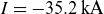 $I = -35.2\, {\rm kA}$
. To find the umbilic coil shape, coil current and the corresponding plasma shape that minimises the normal field error
$I = -35.2\, {\rm kA}$
. To find the umbilic coil shape, coil current and the corresponding plasma shape that minimises the normal field error
 $\boldsymbol{B}\boldsymbol{\cdot }\hat {\boldsymbol{n}}$
and the total pressure across the plasma boundary, we combine the objectives defined in (3.8) and (4.1) in a process known as single-stage optimisation. We solve
$\boldsymbol{B}\boldsymbol{\cdot }\hat {\boldsymbol{n}}$
and the total pressure across the plasma boundary, we combine the objectives defined in (3.8) and (4.1) in a process known as single-stage optimisation. We solve
 \begin{align} &\min (\mathcal{F}_{\text{stage-one}} + \mathcal{F}_{\text{stage-two}}), \quad \textrm {s.t.} \ \boldsymbol{\nabla }\left (\mu _0 p + \frac {B^2}{2}\right ) - \boldsymbol{B}\boldsymbol{\cdot }\boldsymbol{\nabla }\boldsymbol{B} = 0,\quad \psi _{\mathrm{b}} = \psi _{\mathrm{b}0},\nonumber \\ & p = p_{0}(\psi ),\quad I = I_0(\psi ), \end{align}
where
 $\psi _{\mathrm{b}0}$
is the user-provided enclosed toroidal flux by the boundary and
$\psi _{\mathrm{b}0}$
is the user-provided enclosed toroidal flux by the boundary and
 $p_0(\psi )$
and
$p_0(\psi )$
and
 $I_0(\psi )$
are the pressure and toroidal current profiles. The optimisable set of parameters is
$I_0(\psi )$
are the pressure and toroidal current profiles. The optimisable set of parameters is
 $\hat {\boldsymbol{p}} \in \{R_{\mathrm{b}, mn}, Z_{\mathrm{b}, mn}, a_k, X_n, Y_n, Z_n, I_{\mathrm{umbilic}}\}$
, where
$\hat {\boldsymbol{p}} \in \{R_{\mathrm{b}, mn}, Z_{\mathrm{b}, mn}, a_k, X_n, Y_n, Z_n, I_{\mathrm{umbilic}}\}$
, where
 $X_n, Y_n, Z_n$
are the Fourier coefficients that determine the shape of the umbilic coil. The coilset and free-boundary solution are presented in figure 13. After optimisation, the normalised
$X_n, Y_n, Z_n$
are the Fourier coefficients that determine the shape of the umbilic coil. The coilset and free-boundary solution are presented in figure 13. After optimisation, the normalised
 $\mathrm{max}(\boldsymbol{B}\boldsymbol{\cdot }\hat {\boldsymbol{n}}) \lt 0.5\,\%$
and the total pressure difference is
$\mathrm{max}(\boldsymbol{B}\boldsymbol{\cdot }\hat {\boldsymbol{n}}) \lt 0.5\,\%$
and the total pressure difference is
 $\lt 0.1\,\%$
. Because we allow the boundary shape to change, we have less control over the curvature along the umbilic edge, so there is a lot of variation. The curvature along the edge lies in the range
$\lt 0.1\,\%$
. Because we allow the boundary shape to change, we have less control over the curvature along the umbilic edge, so there is a lot of variation. The curvature along the edge lies in the range
 $\kappa _{2, \rho } \in [-25, -13]\, {\rm m}^{-1}$
with the average curvature
$\kappa _{2, \rho } \in [-25, -13]\, {\rm m}^{-1}$
with the average curvature
 $\mathrm{avg}(\kappa _{2, \rho }) = -8\, {\rm m}^{-1}$
. The neoclassical transport coefficient
$\mathrm{avg}(\kappa _{2, \rho }) = -8\, {\rm m}^{-1}$
. The neoclassical transport coefficient
 ${\epsilon _{\mathrm{eff}}}^{3/2} \lt 0.001$
implies that the magnetic field is still omnigenous. Finally, we calculate the rotational transform profile of the optimised equilibrium to quantify the effect of the umbilic coil in figure 14.
${\epsilon _{\mathrm{eff}}}^{3/2} \lt 0.001$
implies that the magnetic field is still omnigenous. Finally, we calculate the rotational transform profile of the optimised equilibrium to quantify the effect of the umbilic coil in figure 14.
Coilset and free-boundary solution for the case where the current in the umbilic coil is in the same direction as the plasma current. The current carried by the umbilic coil is
 $I_{\mathrm{umbilic}} = -3.1\,{\rm kA}$
. All coils but the umbilic coil are axisymmetric.
$I_{\mathrm{umbilic}} = -3.1\,{\rm kA}$
. All coils but the umbilic coil are axisymmetric.

The total rotational transform profiles and the contribution from shaping and plasma current. The non-axisymmetric shaping is purely a consequence of the umbilic coil which contributes to approximately
 $5\,\%$
of the total rotational transform in the edge.
$5\,\%$
of the total rotational transform in the edge.

The effect on the rotational transform profile due to the umbilic coil rises sharply as we move towards the edge. Therefore, it is possible that outside the plasma boundary the umbilic coil is able to affect the total magnetic field in such a way that it forms an X-point.
6. Conclusions and future work
This paper has explored the physical properties of USs. In § 3, we defined the umbilic parametrisation, approximated it using DESC and solved the ideal MHD equation inside the enclosed volume. In § 4, we developed vacuum and finite-
 $\beta$
stellarators by simultaneously optimising the umbilic edge and the boundary shape using the DESC optimisation suite. We designed coils for the vacuum case, and traced fieldlines in the edge of the US131 stellarator before and after adding a current source at the magnetic axis, to simulate a plasma fluctuation. Even though we do not see a perfectly sharp X-point (X-line) and well-defined fieldline structure like in a tokamak, the high-curvature edges could be a favourable location to place divertors and are robust to internal plasma fluctuations. We found that the optimised omnigenous umbilic designs do not possess a specific helicity regardless of the low-ripple transport, which could be a way to generate piecewise-omnigenous equilibria. As a final demonstration, in § 5, we propose an experiment to modify the Columbia HBT-EP experiment to an umbilic design by adding an
$\beta$
stellarators by simultaneously optimising the umbilic edge and the boundary shape using the DESC optimisation suite. We designed coils for the vacuum case, and traced fieldlines in the edge of the US131 stellarator before and after adding a current source at the magnetic axis, to simulate a plasma fluctuation. Even though we do not see a perfectly sharp X-point (X-line) and well-defined fieldline structure like in a tokamak, the high-curvature edges could be a favourable location to place divertors and are robust to internal plasma fluctuations. We found that the optimised omnigenous umbilic designs do not possess a specific helicity regardless of the low-ripple transport, which could be a way to generate piecewise-omnigenous equilibria. As a final demonstration, in § 5, we propose an experiment to modify the Columbia HBT-EP experiment to an umbilic design by adding an
 $m=1, n=1$
helical coil. Using the DESC free-boundary solver, we demonstrate that the umbilic coils are able to cause the originally circular plasma to bulge and form a high-curvature ridge while maintaining omnigenity. By changing the direction of the current in the umbilic coil, we may be able to get an X-point, thereby converting the limited HBT-EP tokamak into a diverted stellarator.
$m=1, n=1$
helical coil. Using the DESC free-boundary solver, we demonstrate that the umbilic coils are able to cause the originally circular plasma to bulge and form a high-curvature ridge while maintaining omnigenity. By changing the direction of the current in the umbilic coil, we may be able to get an X-point, thereby converting the limited HBT-EP tokamak into a diverted stellarator.
The technique of simultaneously optimising a curve and a surface to control the magnitude and position of a sharp edge along a surface extends beyond USs. One can use this method to place and design ridges or regions of high curvature which may be useful for non-resonant divertors (Bader et al. Reference Bader, Hegna, Cianciosa and Hartwell2018b
), as well as these ridges creating preferential pathways for the fieldlines to exit the plasma (Bader et al. Reference Bader, Boozer, Hegna, Lazerson and Schmitt2017). This can be achieved by multiplying a custom function
 $g(\theta )$
to the objective
$g(\theta )$
to the objective
 $f_{\mathrm{umbilic}}$
such that
$f_{\mathrm{umbilic}}$
such that
 $g(\theta ) = 1\quad \forall \quad \theta \in \bigcup _{i} [\theta _{i0}, \theta _{i1}]$
and
$g(\theta ) = 1\quad \forall \quad \theta \in \bigcup _{i} [\theta _{i0}, \theta _{i1}]$
and
 $g(\theta ) = 0$
elsewhere along the umbilic curve, with
$g(\theta ) = 0$
elsewhere along the umbilic curve, with
 $\theta _{i0}, \theta _{i1}$
being optimisable parameters describing the lower and upper limits of regions where low curvature is penalised. This will create a set of continuous but disconnected ridges, just as we observe in non-resonant divertor concepts. This functionality is available in DESC. For an island divertor concept, the rotational transform on the boundary can be fine-tuned using umbilic coils, which could be used to reduce the sensitivity of X-points in the island divertor structure due to changes in the plasma boundary rotational transform. This idea is similar to that of divertor coils in tokamaks and would lead to a predictable strike point pattern.
$\theta _{i0}, \theta _{i1}$
being optimisable parameters describing the lower and upper limits of regions where low curvature is penalised. This will create a set of continuous but disconnected ridges, just as we observe in non-resonant divertor concepts. This functionality is available in DESC. For an island divertor concept, the rotational transform on the boundary can be fine-tuned using umbilic coils, which could be used to reduce the sensitivity of X-points in the island divertor structure due to changes in the plasma boundary rotational transform. This idea is similar to that of divertor coils in tokamaks and would lead to a predictable strike point pattern.
Future work would involve using multiple umbilic coils to ensure plasma stability against low-
 $n$
modes (
$n$
modes (
 $n = 0$
family) and increase the curvature of the ridge, similar to the work on tokamak separatrix by Webster (Reference Webster2009), understanding the strike point pattern and fieldline structure outside the plasma boundary or designing umbilic coils for a case similar to the finite-
$n = 0$
family) and increase the curvature of the ridge, similar to the work on tokamak separatrix by Webster (Reference Webster2009), understanding the strike point pattern and fieldline structure outside the plasma boundary or designing umbilic coils for a case similar to the finite-
 $\beta$
 $\textrm {US}252$
stellarator in § 4.4. It is also important to include MHD and kinetic stability metrics in the optimisation process, especially near the boundary as has been done for tokamaks by Bishop (Reference Bishop1986) and Zheng et al. (Reference Zheng, Kotschenreuther, Waelbroeck and Austin2025) as stability properties can be sensitive close to the high-curvature plasma boundary.
$\textrm {US}252$
stellarator in § 4.4. It is also important to include MHD and kinetic stability metrics in the optimisation process, especially near the boundary as has been done for tokamaks by Bishop (Reference Bishop1986) and Zheng et al. (Reference Zheng, Kotschenreuther, Waelbroeck and Austin2025) as stability properties can be sensitive close to the high-curvature plasma boundary.
Acknowledgements
One of the authors, R.G., enjoyed discussions with M. Zarnstroff, J. Levesque, R. Davies, J.L. Velasco and B. Jang, and gratefully acknowledges the help from S. Lazerson in installing the FIELDLINES code. We also express our gratitude to the referees for their constructive feedback that has improved the overall quality of this paper.
Editor Per Helander thanks the referees for their advice in evaluating this article.
Funding
This work is funded through the SciDAC programme by the US Department of Energy, Office of Fusion Energy Science and Office of Advanced Scientific Computing Research under contract no. DE-AC02-09CH11466, the Hidden Symmetries grant from the Simons Foundation/SFARI (560651) and Microsoft Azure Cloud Computing mini-grant awarded by the Center for Statistics and Machine Learning (CSML), Princeton University. This research also used the Della cluster at Princeton University.
Declaration of interests
M.L. is a consultant for Type One Energy.
Data availability statement
All the data, analysis and post-processing files are freely available in Gaur (Reference Gaur2025). https://zenodo.org/records/15355215.
Appendix A. Calculating principal curvatures
The second principal curvature at a given point on a surface is defined as
 \begin{equation} \kappa _{2, \rho } = \min \left \{k:\det \left [\begin{array}{cc} L_{\mathrm{sff}, \rho } - k E & M_{\mathrm{sff}, \rho } - k F \\ M_{\mathrm{sff}, \rho } - k F & N_{\mathrm{sff}, \rho } - k G \end{array}\right ] = 0\right \}\!, \end{equation}
where
 \begin{equation} \begin{split} E &= \frac {\partial \boldsymbol{x}}{\partial \zeta } \boldsymbol{\cdot }\frac {\partial \boldsymbol{x}}{\partial \zeta },\quad F = \frac {\partial \boldsymbol{x}}{\partial \zeta } \boldsymbol{\cdot }\frac {\partial \boldsymbol{x}}{\partial \theta },\quad G = \frac {\partial \boldsymbol{x}}{\partial \theta } \boldsymbol{\cdot }\frac {\partial \boldsymbol{x}}{\partial \theta }, \\ L_{\mathrm{sff}, \rho } &= \frac {\partial ^2 \boldsymbol{x}}{\partial \theta ^2} \boldsymbol{\cdot }\frac {\boldsymbol{\nabla }\rho }{|\boldsymbol{\nabla }\rho |}, \quad M_{\mathrm{sff}, \rho } = \frac {\partial ^2 \boldsymbol{x}}{\partial \theta \partial \zeta } \boldsymbol{\cdot }\frac {\boldsymbol{\nabla }\rho }{|\boldsymbol{\nabla }\rho |}, \quad N_{\mathrm{sff}, \rho } = \frac {\partial ^2 \boldsymbol{x}}{\partial \zeta ^2} \boldsymbol{\cdot }\frac {\boldsymbol{\nabla }\rho }{|\boldsymbol{\nabla }\rho |} \end{split} \end{equation}
are the metric coefficients corresponding to the first and second fundamental forms. The user-specified values
 $\kappa _{2, \mathrm{bound1}}, \kappa _{2, \mathrm{bound2}}$
define the limits on the curvature. Using this objective, we impose a maximum and minimum value on
$\kappa _{2, \mathrm{bound1}}, \kappa _{2, \mathrm{bound2}}$
define the limits on the curvature. Using this objective, we impose a maximum and minimum value on
 $\kappa _{2, \rho }$
that helps us impose a sharp curvature along the umbilic edge.
$\kappa _{2, \rho }$
that helps us impose a sharp curvature along the umbilic edge.
Appendix B. Form of various objectives
All the objectives with bounds are defined as
 \begin{eqnarray} f_{\mathrm{obj}} = \mathrm{ReLU}(\max (\textrm {obj} - \textrm {obj}_{\mathrm{bound1}}, \textrm {obj} - \textrm {obj}_{\mathrm{bound2}})). \end{eqnarray}
In this paper, such a term is used to penalise the aspect ratio, the rotational transform and the second principal curvature
 $\kappa _{2, \rho }$
along the umbilic edge.
$\kappa _{2, \rho }$
along the umbilic edge.
For the effective ripple objective explained in Unalmis et al. (Reference Unalmis, Gaur, Conlin, Panici and Kolemen2024) and the omnigenity objective implemented by Dudt et al. (Reference Dudt, Goodman, Conlin, Panici and Kolemen2024), we do not use any bounds and try to reduce the magnitude of these quantities as much as possible. The exact definitions are given in the respective papers.
Appendix C. Piecewise omnigenity in umbilic configurations
In this appendix, we plot the normalised second adiabatic invariant
 $\mathcal{J}_{\parallel } = \int _{l_1}^{l_2} \textrm{d}l\, v_{\parallel }/(2\pi R_0)$
as a function of the fieldline label
$\mathcal{J}_{\parallel } = \int _{l_1}^{l_2} \textrm{d}l\, v_{\parallel }/(2\pi R_0)$
as a function of the fieldline label
 $\alpha$
and the inverse pitch angle
$\alpha$
and the inverse pitch angle
 $1/\lambda \equiv E/\mu$
. We calculate
$1/\lambda \equiv E/\mu$
. We calculate
 $\mathcal{J}_{\parallel }(\alpha , 1/\lambda )$
on a single flux surface on which the neoclassical transport coefficient
$\mathcal{J}_{\parallel }(\alpha , 1/\lambda )$
on a single flux surface on which the neoclassical transport coefficient
 $\epsilon _{\mathrm{eff}}^{3/2} \leqslant 0.001$
. This is done for both the US131 vacuum and US252 finite-β equilibria presented in §§ 4.1 and 4.4, respectively. To highlight their difference, we also plot
$\epsilon _{\mathrm{eff}}^{3/2} \leqslant 0.001$
. This is done for both the US131 vacuum and US252 finite-β equilibria presented in §§ 4.1 and 4.4, respectively. To highlight their difference, we also plot
 $\mathcal{J}_{\parallel }$
for a poloidally omnigenous (or QI)
$\mathcal{J}_{\parallel }$
for a poloidally omnigenous (or QI)
 $n_{\textrm {FP}}=1$
vacuum equilibrium taken from the DESC omnigenity database (Gaur et al. Reference Gaur, Dudt, Conlin, Panici, Unalmis and Kolemen2023). Comparison is shown in figure 15.
$n_{\textrm {FP}}=1$
vacuum equilibrium taken from the DESC omnigenity database (Gaur et al. Reference Gaur, Dudt, Conlin, Panici, Unalmis and Kolemen2023). Comparison is shown in figure 15.
Plots of the second adiabatic invariant
 $\mathcal{J}_{\parallel }(\alpha , 1/\lambda )$
and
$\mathcal{J}_{\parallel }(\alpha , 1/\lambda )$
and
 $|B|$
contours for three equilibria with
$|B|$
contours for three equilibria with
 $\epsilon _{\mathrm{eff}}^{3/2} \approx 0.001$
. For a close-to-perfect omnigenous equilibrium
$\epsilon _{\mathrm{eff}}^{3/2} \approx 0.001$
. For a close-to-perfect omnigenous equilibrium
 $\partial _{\alpha }\mathcal{J}_{\parallel }$
is close to zero for most values of
$\partial _{\alpha }\mathcal{J}_{\parallel }$
is close to zero for most values of
 $1/\lambda$
, as seen in (c). However, for (a, b) there are multiple distinct values of
$1/\lambda$
, as seen in (c). However, for (a, b) there are multiple distinct values of
 $\mathcal{J}_{\parallel }$
, discontinuous in
$\mathcal{J}_{\parallel }$
, discontinuous in
 $\alpha$
, a necessary condition for piecewise omnigenity.
$\alpha$
, a necessary condition for piecewise omnigenity.

For a perfect, non-piecewise-omnigenous stellarator
 $\partial _{\alpha }(\mathcal{J}_{\parallel }) = 0$
, implying that
$\partial _{\alpha }(\mathcal{J}_{\parallel }) = 0$
, implying that
 $\mathcal{J}_{\parallel }$
is continuous and constant in
$\mathcal{J}_{\parallel }$
is continuous and constant in
 $\alpha$
for almost every
$\alpha$
for almost every
 $1/\lambda$
. Moreover, the distinct
$1/\lambda$
. Moreover, the distinct
 $\mathcal{J}_{\parallel }$
can be written as a linear sum such that the total
$\mathcal{J}_{\parallel }$
can be written as a linear sum such that the total
 $\mathcal{J}_{\parallel }$
for a value of the inverse pitch vanishes. However, for the umbilic configurations in this paper, especially the US131 vacuum stellarator, despite a low effective ripple (good omnigenity), we clearly see that
$\mathcal{J}_{\parallel }$
for a value of the inverse pitch vanishes. However, for the umbilic configurations in this paper, especially the US131 vacuum stellarator, despite a low effective ripple (good omnigenity), we clearly see that
 $\mathcal{J}_{\parallel }$
is discontinuous in
$\mathcal{J}_{\parallel }$
is discontinuous in
 $\alpha$
for most of the inverse pitch values and
$\alpha$
for most of the inverse pitch values and
 $\tilde {\mathcal{J}}_{\parallel , \mathrm{I}} \approx \tilde {\mathcal{J}}_{\parallel , \mathrm{II}} \approx 0.5 \tilde {\mathcal{J}}_{\parallel , \mathrm{III}}$
. This supports our claim that the umbilic stellarator US131 is piecewise-omnigenous, especially at large values of the inverse pitch. US252 seems to be piecewise-omnigenous but the structure of
$\tilde {\mathcal{J}}_{\parallel , \mathrm{I}} \approx \tilde {\mathcal{J}}_{\parallel , \mathrm{II}} \approx 0.5 \tilde {\mathcal{J}}_{\parallel , \mathrm{III}}$
. This supports our claim that the umbilic stellarator US131 is piecewise-omnigenous, especially at large values of the inverse pitch. US252 seems to be piecewise-omnigenous but the structure of
 $\tilde {\mathcal{J}_{\parallel }}$
is more complicated than that discussed by Velasco et al. (Reference Velasco, Calvo, Escoto, Sánchez, Thienpondt and Parra2024).
$\tilde {\mathcal{J}_{\parallel }}$
is more complicated than that discussed by Velasco et al. (Reference Velasco, Calvo, Escoto, Sánchez, Thienpondt and Parra2024).
Appendix D. Details of the HBT-EP equilibrium
The original HBT-EP equilibrium is a shifted-circle equilibrium with a major radius
 $R_0 = 0.94\, {\rm m}$
, minor radius
$R_0 = 0.94\, {\rm m}$
, minor radius
 $a_0 = 0.125\, {\rm m}$
(aspect ratio
$a_0 = 0.125\, {\rm m}$
(aspect ratio
 $A = 7.52$
) with
$A = 7.52$
) with
 $\beta = 0.5\,\%$
and a plasma current
$\beta = 0.5\,\%$
and a plasma current
 $I = -35.2\, {\rm kA}$
. The pressure and rotational transform profiles are given in figure 16. The initial equilibrium was tested to be stable against
$I = -35.2\, {\rm kA}$
. The pressure and rotational transform profiles are given in figure 16. The initial equilibrium was tested to be stable against
 $n = 1$
kink modes using the DCON-2D (Glasser Reference Glasser2016) stability code.
$n = 1$
kink modes using the DCON-2D (Glasser Reference Glasser2016) stability code.
Profiles of the initial HBT-EP equilibrium.

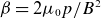


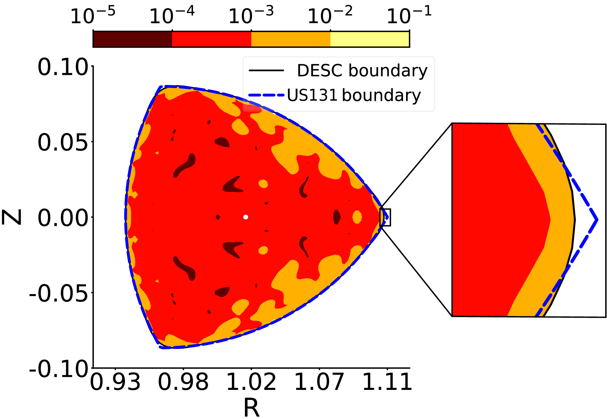


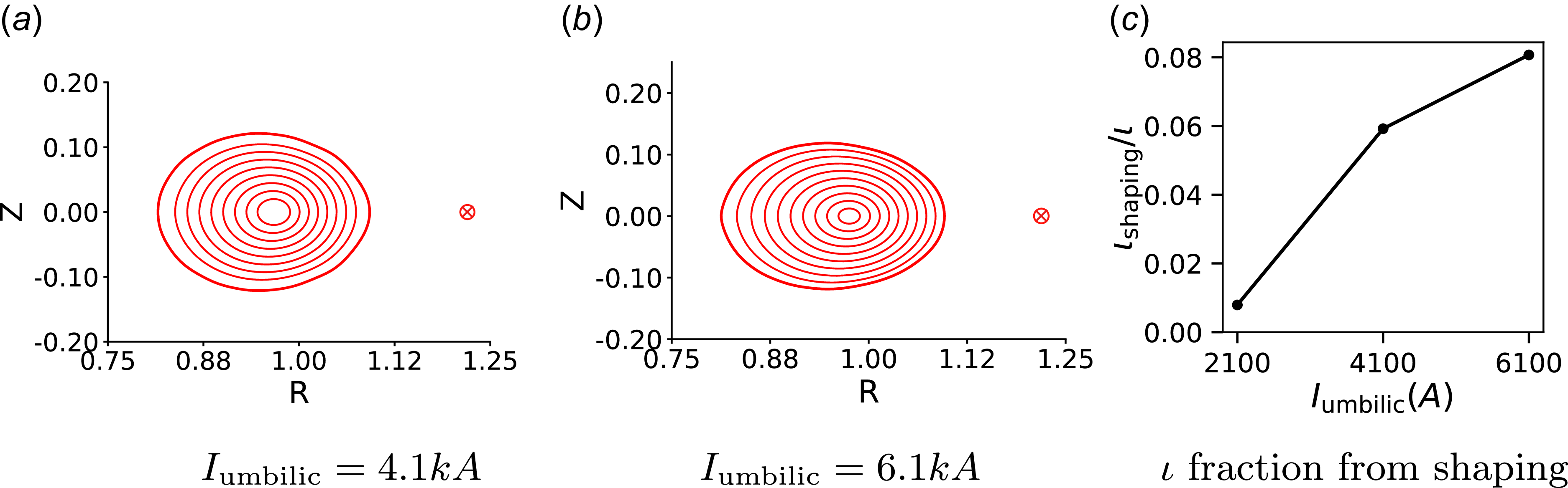


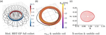


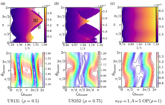


 Open access