


1. Introduction
The phenomenon of propagation of steady periodic waves over a planar seabed is one of the oldest and most fascinating problems in fluid dynamics, and dates back to the pioneering work of Stokes (Reference Stokes1847). Beyond the interesting and challenging mathematical aspects, it embraces a wide variety of physical aspects (for example, the different behaviours over different wave depths, the interplay between dispersion and nonlinearity, the interactions with currents) that are important in many applied fields, like coastal and maritime engineering, naval engineering and environmental sciences. Despite the enormous amount of contributions on this subject, some aspects of wave propagation still deserve a dedicated study, especially in the field lying between practical applications and theory. The present work is dedicated to this latter aspect, providing a semi-analytical approach to the modelling of wave propagating over planar seabed that is accurate and, at the same time, provides solutions that are of practical interest for applications (e.g. numerical simulations and benchmarking). To better characterize the framework where the present work lies, we describe briefly the principal contributions in this field of research.
The analytical approach proposed by Stokes (Reference Stokes1847, Reference Stokes1880) is based on the use of a perturbation expansion in a small parameter (the wave steepness) and applies to waves propagating over finite up to infinite depth. The third-order solution highlights some interesting features, like the increase of the wave celerity (namely, the wave translational velocity) as a function of the increase of the wave amplitude and the existence of a drift velocity in the same direction as the wave propagation. The main drawback of the Stokes approach is that the solution becomes singular as shallower depths are considered. Higher-order expansions (up to fifth-order) increase the range of validity of the Stokes solution slightly, but confirm the above features (see Fenton Reference Fenton1985).
The failure of the Stokes expansion is essentially caused by the singularity in shallow depths of the linear operator arising from the perturbation approach. In this regime of motion (which is characterized by the propagation of long waves in comparison with the still-water depth), the variations of the wave quantities are rather slow and, consequently, their order of magnitude is small. This results in a nonlinear interaction between the lowest mode of the steady periodic wave and its higher modes. The perturbation expansion at the basis of the cnoidal wave theory essentially stems from the above considerations and stands as a complementary approach in comparison to that used to derive the Stokes waves. At each order of the expansion, a nonlinear equation is obtained, whose solution is capable of describing the wave propagation up to the limit of infinite wavelength (i.e. solitary waves; Fenton Reference Fenton1972). On the other hand, the solution becomes inaccurate when the water depth becomes deeper, and higher-order solutions just mitigate this issue (see Fenton Reference Fenton1979).
In summary, the attainment of an exact or approximate analytical solution for the wave propagation in all the regimes of motion (i.e. shallow, intermediate and deep water) is still an open field of research, and despite the huge literature on this topic, no global analytical solution is currently available, to the author's knowledge.
The lack of such a global solution also results in a problem in practical applications, since the modelling of travelling waves in intermediate water often lies in the grey region where both the fifth-order theories (namely, Stokes and cnoidal waves) approach their own limits of validity.
The above considerations led many researchers to develop semi-analytical methods, that is, approaches where analytical modelling is provided up to a certain point, and a final part is left to numerical evaluation. In this case, explicit analytical solutions are generally not available but, in turn, it is possible to overcome many of the issues affecting the perturbation expansions and maintain a rigorous mathematical framework and an insight into the main physical aspects. To this class belong, for example, the works of Schwartz (Reference Schwartz1974), Williams (Reference Williams1981), Liao & Cheung (Reference Liao and Cheung2003), Tao, Song & Chakrabarti (Reference Tao, Song and Chakrabarti2007), Dyachenko, Lushnikov & Korotkevich (Reference Dyachenko, Lushnikov and Korotkevich2016) and Zhong & Liao (Reference Zhong and Liao2018). Some of those are devoted to the study of waves of maximum amplitude (also called waves of extreme height). These waves (whose existence in nature has been only conjectured) are predicted by the governing equations and are characterized by interesting specific features (both mathematical and physical), as the occurrence of a sharp angle at the crest (i.e. a singularity at the free surface). As shown in Henry (Reference Henry2006), Constantin (Reference Constantin2006, Reference Constantin2012) and Constantin & Escher (Reference Constantin and Escher2007), such a point behaves as an apparent stagnation point in the frame of reference moving with the wave speed, i.e. the velocity at the crest is null whereas the fluid particles are actually moving.
Despite a consistent number of theoretical works on extreme waves (Grant Reference Grant1973; Norman Reference Norman1974; Longuet-Higgins Reference Longuet-Higgins1977; Toland Reference Toland1978; Amick, Fraenkel & Toland Reference Amick, Fraenkel and Toland1982; Plotnikov Reference Plotnikov2002; Plotnikov & Toland Reference Plotnikov and Toland2004), their modelling is, at present, possible only through semi-analytical methods, whereas fifth-order wave theories cannot adequately represent such a high nonlinear phenomenon.
The present work belongs to the above-mentioned class of semi-analytical methods and is aimed at providing a fast and accurate model for wave propagation in all the regimes of motion, up to the limit of maximum-amplitude waves. The main target is to give a contribution to the theoretical description of steady periodic waves and to fill the gap between the theories in deep- and shallow-water conditions, supplying a reliable tool for practical applications (i.e. wave modelling, numerical benchmarking, etc.). The iterative scheme proposed in this work has been defined starting from the integral equation of Byatt-Smith (Reference Byatt-Smith1970), which represents a rearrangement of the governing system of equations into a single equation in a suitable hodograph space. Special attention has been devoted to the physical characterization of the main parameters that arise in such a mathematical framework. The proposed iterative approach is intrinsically nonlinear and, consequently, is not affected by the singularity in the shallow-water limit that characterizes the linear operator of the Stokes wave.
The use of the integral equation of Byatt-Smith (Reference Byatt-Smith1970) is motivated by its simple and compact representation of the wave problem that allows for a straightforward definition of the wave parameters and of the iterative scheme itself. Strangely, such an equation has received little attention in the literature, and to the author's knowledge, no theoretical findings can be enumerated for it at present. Incidentally, we highlight that other integral equations for steady waves have been proposed previously, as in in the pioneering works by Nekrasov (Reference Nekrasov1921, Reference Nekrasov1928). In this latter case, a significant number of theoretical contributions exist (the interested reader can find an exhaustive summary of the literature on Nekrasov's equations in Kuznetsov Reference Kuznetsov2021).
As a preparatory step to the definition of the iterative scheme, a study on the geometrical wave parameters is tackled in § 2 in order to define a global spatial scale associated with the vertical dynamics, that is, a significant length that represents the region where the fluid motion is essentially different from zero in all the regimes of motion. The use of such a scale allows for a global characterization of the solution without falling into a bias caused by the dependence on shallow- or deep-water lengths. It also facilitates the description of the phenomenon of wave propagation as a whole. Hence §§ 3 and 4 introduce the governing equation and the integral equation of Byatt-Smith (Reference Byatt-Smith1970), and § 5 describes the iterative scheme. Finally, § 6 shows the outputs of the proposed scheme and the comparisons with the existing analytical solutions.
2. A global scaling for water waves
The phenomenon of wave propagation is characterized and therefore described by means of three spatial scales: a horizontal length scale  $x_0^*$ (related to the wavelength $L^*$), the wave amplitude $a_0^*$ (half wave height), and the reference water depth $h_0^*$ in the vertical direction. Using these quantities, it is possible to define the following dimensionless numbers:
 \begin{equation} \bar{\mu} = \frac{h_0^*}{x_0^*},\quad \bar{\epsilon} = \frac{a_0^*}{h_0^*},\quad \bar{\sigma} = \frac{a_0^*}{x_0^*} = \bar{\epsilon} \bar{\mu}. \end{equation}
In particular, the first term, usually called dispersion parameter, is used to identify different regimes of motion: waves travel in shallow-water conditions if  $\bar {\mu } \ll 1$ or in the deep-water regime for $\bar {\mu } \gg 1$. Between these extrema, waves are said to propagate in intermediate depths. Finally, the second and third parameters in (2.1a–c) are called the nonlinearity and steepness parameter, respectively, and characterize the intensity of the wave dynamics.
From the last definition in (2.1a–c), it is clear that it is always possible to choose a pair of the above coefficients and deduce the remaining one. In particular, the pair  $(\bar {\mu }, \bar {\epsilon })$ is used to described wave motion in shallow-water conditions, while the pair $(\bar {\mu }, \bar {\sigma })$ is generally adopted in deep water. The use of different pairs according to the different conditions of propagation is motivated by the fact that neither $\bar {\epsilon }$ nor $\bar {\sigma }$ can represent the wave dynamics globally over the three regimes of motion. In shallow depths, the condition $\bar {\mu } \ll 1$ (long waves) leads to $\bar {\sigma } = \bar {\mu } \bar {\epsilon } \ll \bar {\epsilon }$. This, along with the assumption of non-breaking waves (i.e. $\bar {\epsilon } \ll 1$), implies that the parameter $\bar {\sigma }$ is extremely small and, consequently, is not significant for the flow dynamics. The opposite occurs in deep water, where $\bar {\mu } \gg 1$ (short waves) leads to $\bar {\epsilon } = \bar {\sigma }/ \bar {\mu } \ll \bar {\sigma }$. Again, the assumption that waves are non-breaking (i.e. $\bar {\sigma } \ll 1$ in this case) implies that $\bar {\epsilon }$ is not representative of the flow dynamics in deep water.
The definition of a global scaling across the regimes of motion is therefore the first step to derive a solution for waves of permanent shape travelling over a generic depth. The above considerations led us to introduce a further spatial scale, denoted  $z_0^*$, that represents the scale associated with the vertical dynamics, that is, the length of the region where the fluid motion is essentially different from zero. Generally, this is a fraction of the wavelength in deep water, while it becomes comparable with the water depth in shallow-water conditions. Since $z_0^*$ is a derived quantity (namely, it depends on the solution itself), it must depend on the remaining vertical scales, i.e. $a_0^*$ and $h_0^*$. This implies the existence of the functional relation
 \begin{equation} \frac{z_0^*}{x_0^*} = f\left(\frac{a_0^*}{x_0^*}, \frac{h_0^*}{x_0^*}\right) = f\left(\bar{\sigma},\bar{\mu}\right). \end{equation}
Since we restrict our analysis to non-breaking waves, we require  $\bar {\sigma } \ll 1$ in deep water (where $1 \ll \bar {\mu }$) and $\bar {\epsilon } \ll 1$ in shallow water (where $\bar {\mu } \ll 1$). The former pair of inequalities implies $\bar {\sigma } \ll 1 \ll \bar {\mu }$, while the latter pair leads to $\bar {\sigma } = \bar {\epsilon } \bar {\mu } \ll \bar {\mu } \ll 1$. Hence for non-breaking waves, $\bar {\sigma } \ll \bar {\mu }$ holds true over all the regimes of motion. The above findings suggest that the dimensionless parameter $\bar {\mu }$ is the most meaningful to describe the relevant vertical scale for the wave propagation phenomenon. As a consequence, (2.2) can be simplified as
 \begin{equation} \frac{z_0^*}{x_0^*} \simeq f\left(0, \bar{\mu} \right) = \hat{f}(\bar{\mu}). \end{equation}
Starting from this result, we introduce new operative dimensionless parameters in analogy with those described in (2.1a–c):
 \begin{equation} \mu = \frac{z_0^*}{x_0^*} = \hat{f}(\bar{\mu}),\quad \epsilon = \frac{a_0^*}{z_0^*}. \end{equation}
Note that there is no need to specify an equivalent definition involving  $\bar {\sigma }$, since $\bar {\sigma } = \bar {\epsilon } \bar {\mu } = \epsilon \mu$. The most natural requirement for $z_0^*$ is
 \begin{equation} z_0^* \rightarrow
\left\{ \begin{array}{@{}ll} h_0^* & \textrm{for}\ \bar{\mu}
\rightarrow 0, \\ x_0^* & \textrm{for}\
\bar{\mu} \rightarrow +\infty,
\end{array}\right.\quad \Rightarrow \quad \epsilon
\rightarrow \left\{\begin{array}{@{}ll} \bar{\epsilon} &
\textrm{for}\ \bar{\mu} \rightarrow 0, \\
\bar{\sigma} & \textrm{for}\ \bar{\mu} \rightarrow
+\infty. \end{array} \right.
\end{equation}
\begin{equation} z_0^* \rightarrow
\left\{ \begin{array}{@{}ll} h_0^* & \textrm{for}\ \bar{\mu}
\rightarrow 0, \\ x_0^* & \textrm{for}\
\bar{\mu} \rightarrow +\infty,
\end{array}\right.\quad \Rightarrow \quad \epsilon
\rightarrow \left\{\begin{array}{@{}ll} \bar{\epsilon} &
\textrm{for}\ \bar{\mu} \rightarrow 0, \\
\bar{\sigma} & \textrm{for}\ \bar{\mu} \rightarrow
+\infty. \end{array} \right.
\end{equation}
As a consequence of this requirement,  $z_0^*$ remains finite over all the regimes of motion, while $h_0^*$ and $x_0^*$ go to infinity in deep- and shallow-water conditions, respectively.Further, $\epsilon$ always tends to the most ‘significant’ parameter according to the specific regime of motion. The above limits also imply the following asymptotic behaviours for $\mu$:
 \begin{equation} \mu =
\hat{f}(\bar{\mu}) \simeq \left\{\begin{array}{@{}ll}
\bar{\mu} & \textrm{for}\ \bar{\mu} \rightarrow 0,
\\ 1 & \textrm{for}\ \bar{\mu} \rightarrow
+\infty. \end{array}\right.
\end{equation}
\begin{equation} \mu =
\hat{f}(\bar{\mu}) \simeq \left\{\begin{array}{@{}ll}
\bar{\mu} & \textrm{for}\ \bar{\mu} \rightarrow 0,
\\ 1 & \textrm{for}\ \bar{\mu} \rightarrow
+\infty. \end{array}\right.
\end{equation}
At this point, we have to specify a choice for both  $z_0^*$ and $x_0^*$. The most natural choice for $z_0^*$ comes from the first-order solution for the wave celerity in Stokes waves, $c_{s,0}^*$, which is generally regarded as a reliable approximation over all the three regimes of motion. In particular, this reads
 \begin{equation} \left( c_{s,0}^* \right)^2 = g^*\,\frac{\tanh( \kappa_0^* h_0^* )}{\kappa_0^*}, \end{equation}
where  $\kappa _0^* = 2 {\rm \pi}/ L^*$ is the wavenumber, and $g^*$ is the gravity acceleration. Defining the scale for the wave celerity as $\sqrt {g^* z_0^*}$, we require
 \begin{equation} \frac{( c_{s,0}^* )^2}{g^* z_0^* } = 1\quad \Rightarrow \quad \mu = \frac{\tanh( \kappa_0^* h_0^* )}{\kappa_0^* x_0^*}. \end{equation}
Then, choosing  $x_0^* = 1/\kappa _0^*$, we finally obtain
 \begin{equation} \mu = \tanh \left(\bar{\mu} \right), \end{equation}
which is consistent with the functional definition of  $\mu$ given in (2.4a,b), and with the requirements in (2.6).
Using (2.9), it is possible to give simple theoretical definitions of the shallow- and deep-water regimes. Specifically, based on the asymptotic behaviours of  $\mu$, we introduce the quantities:
 $$\begin{gather} \bar{\mu}_S = \sup \left\{\bar{\mu}\ \textrm{such that}\ \left|\bar{\mu} - \tanh\left(\bar{\mu}\right)\right| < 0.01 \right\}, \end{gather}$$
 $$\begin{gather}\bar{\mu}_D = \inf \left\{\bar{\mu}\ \textrm{such that}\ \left|1 - \tanh\left(\bar{\mu} \right)\right| < 0.01\right\}. \end{gather}$$
Accordingly, we say that the shallow-water regime occurs for  $\bar {\mu } < \bar {\mu }_S$, and the deep-water regime for $\bar {\mu } > \bar {\mu }_D$. For practical applications, these quantities can be approximated by $\bar {\mu }_S \simeq {\rm \pi}/10$ and $\bar {\mu }_D \simeq 5 {\rm \pi}/6$. Remarkably, these values are close to those usually adopted in the literature (see, for example, Dean & Dalrymple Reference Dean and Dalrymple1991, pp. 64–65). Figure 1(a) displays $\mu$ as a function of $\bar {\mu }$, and the values of $\bar {\mu }_S$ and $\bar {\mu }_D$. Conversely, figure 1(b) shows the behaviours of the parameters $\bar {\sigma }$ and $\bar {\epsilon }$ as functions of $\mu$ for a chosen value of $\epsilon$ (namely, $\epsilon = 0.25$). In particular, using the definitions in (2.4a,b) and (2.9), we obtain
 \begin{equation} \bar{\sigma} = \epsilon \mu,\quad \bar{\epsilon} = \frac{\epsilon \mu}{\textrm{arctanh}(\mu)}. \end{equation}
Figure 1 confirms the fact that neither  $\bar {\sigma }$ nor $\bar {\epsilon }$ can be used as reference parameter for the description of the wave propagation over the three regimes of motion.
(a) Parameter  $\mu$ as a function of $\bar {\mu }$ (solid line). The dashed lines indicate the values of $\bar {\mu }_S$ and $\bar {\mu }_D$, while the dotted lines denote the asymptotic behaviours of $\mu$. (b) Parameters $\bar {\sigma }$ and $\bar {\epsilon }$ as functions of $\mu$ for $\epsilon = 0.25$.

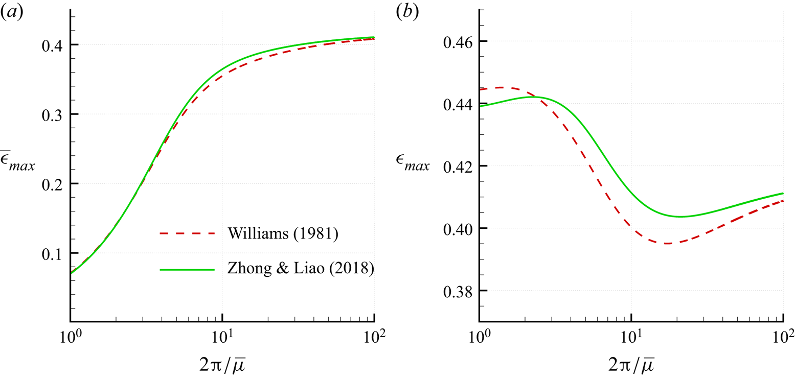
To give an example of the physical meaning and utility of the scale  $\epsilon$, we consider the propagation of waves of maximum amplitude. The existence of these waves is conjectured based on numerical and theoretical results even though, from a practical point of view, waves in the real world are expected to break before reaching their theoretical maximum amplitude. Through the years, different works have been devoted to the derivation of relations for the maximum amplitude of a wave propagating over a certain water depth. Among the most widespread, we report here the relation provided in Fenton (Reference Fenton1990) based on the results by Williams (Reference Williams1981),
 \begin{equation} \bar{\epsilon}_{max} = \frac{1}{2} \left(\frac{\displaystyle 0.141063 \zeta + 0.0095721 \zeta^2 + 0.0077829 \zeta^3}{\displaystyle 1 + 0.0788340 \zeta + 0.0317567 \zeta^2 + 0.0093407 \zeta^3}\right), \end{equation}
and the expression proposed recently by Zhong & Liao (Reference Zhong and Liao2018),
 \begin{equation} \bar{\epsilon}_{max} = \frac{1}{2} \left(\frac{\displaystyle 0.14109 \zeta + 0.00804 \zeta^2 + 0.00949 \zeta^3}{\displaystyle 1 + 0.09671 \zeta + 0.02695 \zeta^2 + 0.01139 \zeta^3}\right), \end{equation}
where  $\zeta = 2 {\rm \pi}/\bar {\mu }$ varies in $[1,100]$. In both the above formulas, the range of variation of $\bar {\epsilon }_{max}$ is quite large. In Williams (Reference Williams1981), $\bar {\epsilon }_{max}$ varies from $0.0707$ for $\zeta = 1$ (deep water) to $0.4082$ for $\zeta = 100$ (shallow water), and similar values are predicted by Zhong & Liao (Reference Zhong and Liao2018), namely $0.0699$ for $\zeta = 1$, and $0.4106$ for $\zeta = 100$ (see figure 2a). Conversely, the range of variation becomes much more narrow if we use the new scaling and introduce $\epsilon _{max} = (\bar {\mu }/\mu ) \bar {\epsilon }_{max}$. As shown in figure 2(b), $\epsilon _{max}$ ranges between $0.395$ and $0.445$. Hence the new scaling represents a significant order of magnitude for the maximum wave amplitude over all the regimes of motion.
Laws for the maximum wave amplitude as proposed by Williams (Reference Williams1981) (dashed lines) and by Zhong & Liao (Reference Zhong and Liao2018) (solid lines), displayed by using the parameters (a)  $\bar {\epsilon }$, and (b) $\epsilon$.
Before proceeding to the next section, we underline that the parameter  $\mu$ in (2.9) was already derived in Kirby (Reference Kirby1998) by following a different approach. In that case, the aim of the work was to remedy an inconsistency in the scaling proposed in Beji (Reference Beji1995). A first application involving the use of the above parameter is reported in Janssen, Herbers & Battjes (Reference Janssen, Herbers and Battjes2006) in the context of spectral models.
3. Governing equations
The dynamics of an inviscid and irrotational free-surface flow over a uniform seabed is described by the following system (in dimensional variables):
 \begin{equation}
\left.\begin{array}{@{}ll@{}} \left.\begin{array}{@{}l@{}l}\phi^*_{z^*} =\eta^*_{t^*} +
\phi^*_{x^*} \eta^*_{x^*}, \\ & \\
\displaystyle{\phi^*_{t^*} + \dfrac{{\phi^*_{x^*}}^{2}}{2}
+ \dfrac{{\phi^*_{z^*}}^{2}}{2} + g^* \eta^*} = B^*,\!\!\!\end{array}\right\} & z^* = \eta^*,\\
\phi^*_{x^* x^*} + \phi^*_{z^* z^*} = 0, \\
\phi^*_{z^*} = 0, & z^* ={-} h_0^*, \end{array}\right\}
\end{equation}
\begin{equation}
\left.\begin{array}{@{}ll@{}} \left.\begin{array}{@{}l@{}l}\phi^*_{z^*} =\eta^*_{t^*} +
\phi^*_{x^*} \eta^*_{x^*}, \\ & \\
\displaystyle{\phi^*_{t^*} + \dfrac{{\phi^*_{x^*}}^{2}}{2}
+ \dfrac{{\phi^*_{z^*}}^{2}}{2} + g^* \eta^*} = B^*,\!\!\!\end{array}\right\} & z^* = \eta^*,\\
\phi^*_{x^* x^*} + \phi^*_{z^* z^*} = 0, \\
\phi^*_{z^*} = 0, & z^* ={-} h_0^*, \end{array}\right\}
\end{equation}
where  $\phi ^*$ is the velocity potential, $\eta ^*$ and $h_0^*$ are the free-surface elevation and the level of the horizontal seabed, $g^*$ is the gravity acceleration, and $B^*$ is the Bernoulli constant. The horizontal and vertical spatial coordinates, namely $(x^*,z^*)$, form a right-handed frame of reference where $z^*$ points upwards and $z^*=0$ indicates the still-water level.
Now let us consider waves that translate with a constant velocity  $c^*$ in the direction of decreasing values of $x^*$. This is equivalent to assuming that all quantities depend on $t^*$ and $x^*$ through the composite variable $x^* + c^* t^*$. Hence the system (3.1) becomes:
 \begin{equation}
\left.\begin{array}{@{}ll@{}} \left.\begin{array}{@{}l@{}l}\phi^*_{z^*} =
\left(\phi^*_{x^*} + c^* \right) \eta^*_{x^*},
\\ & \\
\displaystyle{c^* \phi^*_{x^*} +
\dfrac{{\phi^*_{x^*}}^{2}}{2} +
\dfrac{{\phi^*_{z^*}}^{2}}{2} + g^* \eta^*} = B^*, \!\!\!\end{array}\right\}& z^* = \eta^*,\\
\phi^*_{x^* x^*} + \phi^*_{z^* z^*} = 0, \\
\phi^*_{z^*} = 0, & z^* ={-} h_0^*.
\end{array}\right\} \end{equation}
\begin{equation}
\left.\begin{array}{@{}ll@{}} \left.\begin{array}{@{}l@{}l}\phi^*_{z^*} =
\left(\phi^*_{x^*} + c^* \right) \eta^*_{x^*},
\\ & \\
\displaystyle{c^* \phi^*_{x^*} +
\dfrac{{\phi^*_{x^*}}^{2}}{2} +
\dfrac{{\phi^*_{z^*}}^{2}}{2} + g^* \eta^*} = B^*, \!\!\!\end{array}\right\}& z^* = \eta^*,\\
\phi^*_{x^* x^*} + \phi^*_{z^* z^*} = 0, \\
\phi^*_{z^*} = 0, & z^* ={-} h_0^*.
\end{array}\right\} \end{equation}
The dimensional scaling of the above equations is introduced by using the definitions in (2.4a,b). In particular, we use  $z_0^*$ for both the horizontal and vertical scale, since this length is always finite over all the three regimes of motion. Then we set
 \begin{equation} x^* = z_0^* x,\quad z^* = z_0^* z,\quad t^* = t_0^* t = \sqrt{\frac{z_0^*}{g}}\,t, \end{equation}
and finally,
 \begin{equation} \eta^* = a_0^* \eta,\quad c^* = \sqrt{g z_0^*}\,F,\quad \phi^* = \phi_0^* \phi = c^* z_0^* \phi. \end{equation}
We also introduce the conjugate potential  $\psi ^*$ and the pair of conjugate potentials $\varPhi$ and $\varPsi$ that represent the fluid motion in the frame of reference moving with the wave:
 \begin{equation} \varPhi = \phi + x,\quad \varPsi = \psi + z + H. \end{equation}
Here,  $\psi _0^* = \phi _0^*$ has been used to scale $\varPsi$ and $\psi$, while $H = h_0^*/z_0^*$. As a consequence of the definition in (2.9), it follows that
 \begin{equation} H = \frac{\bar{\mu}}{\tanh(\bar{\mu})} = \frac{\textrm{arctanh}(\mu)}{\mu}. \end{equation}
Then, the system (3.2) becomes:
 \begin{equation}
\left.\begin{array}{@{}ll@{}}\left.\begin{array}{@{}l@{}l} \displaystyle{ \varPhi_z =
\epsilon \dfrac{\textrm{d} \eta}{\textrm{d}\,x}\,\varPhi_x
}, \\ & \\
\displaystyle{\varPhi_x^2 + \varPhi_z^2 = \dfrac{2
\epsilon^2 B + F^2- 2 \epsilon\eta}{F^2},}\!\!\!\end{array}\right\}& z = \epsilon \eta, \\
\varPhi_{x x} + \varPhi_{z z} = 0, \\ \varPhi_z = 0, &
z ={-} H, \end{array}\right\}
\end{equation}
\begin{equation}
\left.\begin{array}{@{}ll@{}}\left.\begin{array}{@{}l@{}l} \displaystyle{ \varPhi_z =
\epsilon \dfrac{\textrm{d} \eta}{\textrm{d}\,x}\,\varPhi_x
}, \\ & \\
\displaystyle{\varPhi_x^2 + \varPhi_z^2 = \dfrac{2
\epsilon^2 B + F^2- 2 \epsilon\eta}{F^2},}\!\!\!\end{array}\right\}& z = \epsilon \eta, \\
\varPhi_{x x} + \varPhi_{z z} = 0, \\ \varPhi_z = 0, &
z ={-} H, \end{array}\right\}
\end{equation}
where  $B = B^*/(u_0^*)^2$, and $u_0^* = \epsilon \sqrt {g^* z_0^*}$ is the reference scale for the horizontal velocity. Before proceeding to the analysis, it is worth noting that $\varPsi$ is constant along the bottom and the free surface (see, for example, Byatt-Smith Reference Byatt-Smith1970). Without any loss of generality, we assume $\varPsi = \varPsi _s$ at the free surface and $\varPsi = 0$ at the bottom.
3.1. The integral equation
In this subsection, we recall briefly the work by Byatt-Smith (Reference Byatt-Smith1970) where the system (3.7) is recast into a single integral equation for the free-surface elevation  $\eta$ through a hodograph transformation.
Balancing the continuity equation, we obtain the scale for the vertical velocity, namely  $w_0^* = u_0^*$. Through this, we write the usual Cauchy–Riemann relations between $\varPhi$ and $\varPsi$:
 \begin{equation}
\left.\begin{array}{@{}l@{}} \varPhi_x = \varPsi_z = U,
\\ \varPhi_z ={-} \varPsi_x = W, \end{array}\right\}
\end{equation}
\begin{equation}
\left.\begin{array}{@{}l@{}} \varPhi_x = \varPsi_z = U,
\\ \varPhi_z ={-} \varPsi_x = W, \end{array}\right\}
\end{equation}
where  $U$ and $W$ are the velocity components in the frame of reference moving with the wave. Now let us consider $(\varPhi, \varPsi )$ as independent variables. Then the following identities hold true:
 \begin{equation} \varPhi \equiv \varPhi\left(x( \varPhi, \varPsi ), z( \varPhi, \varPsi )\right),\quad \varPsi \equiv \varPsi\left(x( \varPhi, \varPsi ), z( \varPhi, \varPsi )\right). \end{equation}
Differentiating by  $\varPhi$, we find
 \begin{equation} 1 \equiv U\,\frac{{\partial} x}{{\partial} \varPhi} +W\,\frac{{\partial} z}{{\partial} \varPhi}, \quad 0 \equiv{-} W\,\frac{{\partial} x}{{\partial} \varPhi} + U\,\frac{{\partial} z}{{\partial} \varPhi}, \end{equation}
and rearranging, we obtain the expressions
 \begin{equation} \frac{{\partial} x}{{\partial} \varPhi} = \frac{U}{ U^2 + W^2},\quad \frac{{\partial} z}{{\partial} \varPhi} = \frac{W}{ U^2 + W^2}, \end{equation}
from which we derive the following equation:
 \begin{equation} \left( \frac{{\partial} x}{{\partial} \varPhi} \right)^2 + \left( \frac{{\partial} z}{{\partial} \varPhi} \right)^2 = \frac{1}{ U^2 + W^2}. \end{equation}
Conversely, differentiating the relations in (3.9a,b) by  $\varPsi$, we find
 \begin{equation} \frac{{\partial} x}{{\partial} \varPsi} ={-} \frac{W}{ U^2 + W^2},\quad \frac{{\partial} z}{{\partial} \varPsi} = \frac{U}{ U^2 + W^2 }, \end{equation}
and by comparison with the equations in (3.11a,b), we derive the Cauchy–Riemann relations in the  $(\varPhi, \varPsi )$-space:
 \begin{equation}
\left.\begin{array}{@{}l@{}}
\displaystyle{\dfrac{{\partial}
x}{{\partial} \varPhi} =
\dfrac{{\partial} z}{{\partial}
\varPsi} }, \\
\displaystyle{\dfrac{{\partial}
x}{{\partial} \varPsi} ={-}
\dfrac{{\partial} z}{{\partial}
\varPhi}}. \end{array}\right\}
\end{equation}
\begin{equation}
\left.\begin{array}{@{}l@{}}
\displaystyle{\dfrac{{\partial}
x}{{\partial} \varPhi} =
\dfrac{{\partial} z}{{\partial}
\varPsi} }, \\
\displaystyle{\dfrac{{\partial}
x}{{\partial} \varPsi} ={-}
\dfrac{{\partial} z}{{\partial}
\varPhi}}. \end{array}\right\}
\end{equation}
Using the results above, we rewrite system (3.7) as
 \begin{equation}
\left.\begin{array}{@{}ll@{}} \left.\begin{array}{@{}l@{}l}
z = \epsilon \eta, \\ & \\
\displaystyle{\left(\dfrac{\textrm{d}\,x_s}{\textrm{d}
\varPhi} \right)^2 } = \displaystyle{\dfrac{F^2}{2
\epsilon^2 B + F^2 - 2 \epsilon \eta} -
\left(\dfrac{\textrm{d} z_s}{\textrm{d} \varPhi}
\right)^2}, \!\!\!\end{array}\right\}&\varPsi = \varPsi_s, \\
\displaystyle{\dfrac{{\partial}^2
z}{{\partial} \varPhi^2} +
\dfrac{{\partial}^2 z}{{\partial}
\varPsi^2} = 0,}\\ z ={-} H & \varPsi = 0,
\end{array}\right\} \end{equation}
\begin{equation}
\left.\begin{array}{@{}ll@{}} \left.\begin{array}{@{}l@{}l}
z = \epsilon \eta, \\ & \\
\displaystyle{\left(\dfrac{\textrm{d}\,x_s}{\textrm{d}
\varPhi} \right)^2 } = \displaystyle{\dfrac{F^2}{2
\epsilon^2 B + F^2 - 2 \epsilon \eta} -
\left(\dfrac{\textrm{d} z_s}{\textrm{d} \varPhi}
\right)^2}, \!\!\!\end{array}\right\}&\varPsi = \varPsi_s, \\
\displaystyle{\dfrac{{\partial}^2
z}{{\partial} \varPhi^2} +
\dfrac{{\partial}^2 z}{{\partial}
\varPsi^2} = 0,}\\ z ={-} H & \varPsi = 0,
\end{array}\right\} \end{equation}
where  $\textrm {d} /\textrm {d} \varPhi$ denotes the derivative along the free surface (i.e. at $\varPsi = \varPsi _s$). Accordingly, the subscript $s$ indicates the variables evaluated at the free surface, namely $x_s = x(\varPhi, \varPsi _s)$ and $z_s = z(\varPhi, \varPsi _s)$. The solution of the Laplace equation for $z( \varPsi,\varPhi )$ that satisfies the impermeability condition at the seabed is
 \begin{equation} z( \varPhi, \varPsi ) ={-} H + \int_{\mathbb{R}} \exp({-{\rm i} y \varPhi})\,A( y) \sinh \left(y \varPsi \right) \textrm{d} y, \end{equation}
and through the Cauchy–Riemann relations in (3.14), we obtain that along  $\varPsi _s$,
 \begin{equation} \frac{\textrm{d}\,x_s}{\textrm{d} \varPhi} = \left( \frac{{\partial} x}{{\partial} \varPhi} \right)_{\varPsi_s} = \left(\frac{{\partial} z}{{\partial} \varPsi} \right)_{\varPsi_s} = \int_{\mathbb{R}} \exp({-{\rm i}\,y\,\varPhi})yA(y) \cosh \left( y \varPsi_s \right) \textrm{d} y. \end{equation}
The expression for  $\textrm{d}\,x_s /\textrm {d} \varPhi$ comes from the second equation of the system (3.15). In particular, we choose the positive sign, since we suppose $x$ and $\varPhi$ to be oriented in the same way. After substitution inside (3.17), we apply the inverse Fourier transform and obtain $A(y)$. Substituting $A(y)$ in (3.16) and evaluating the overall expression at $\varPsi = \varPsi$, we obtain
 \begin{equation}
\left.\begin{array}{@{}l@{}} \displaystyle{\epsilon \eta + H
= \int_{\mathbb{R}} \exp({-{\rm i} y \varPhi})\,
\mathscr{F}^{{-}1}\left[\dfrac{\textrm{d}\,x_s}{\textrm{d}
\varPhi} \right] \dfrac{\tanh\left(y \varPsi_s
\right)}{y}\,\textrm{d} y},\\
\displaystyle{\dfrac{\textrm{d}\,x_s}{\textrm{d} \varPhi} =
\left[\dfrac{F^2}{2 \epsilon^2 B + F^2 - 2 \epsilon \eta }
- \epsilon^2 \left( \dfrac{\textrm{d} \eta}{\textrm{d}
\varPhi} \right)^2\right]^{1/2}},
\end{array}\right\} \end{equation}
\begin{equation}
\left.\begin{array}{@{}l@{}} \displaystyle{\epsilon \eta + H
= \int_{\mathbb{R}} \exp({-{\rm i} y \varPhi})\,
\mathscr{F}^{{-}1}\left[\dfrac{\textrm{d}\,x_s}{\textrm{d}
\varPhi} \right] \dfrac{\tanh\left(y \varPsi_s
\right)}{y}\,\textrm{d} y},\\
\displaystyle{\dfrac{\textrm{d}\,x_s}{\textrm{d} \varPhi} =
\left[\dfrac{F^2}{2 \epsilon^2 B + F^2 - 2 \epsilon \eta }
- \epsilon^2 \left( \dfrac{\textrm{d} \eta}{\textrm{d}
\varPhi} \right)^2\right]^{1/2}},
\end{array}\right\} \end{equation}
where the identity  $z_s(\varPhi ) = \epsilon \,\eta (\varPhi )$ has been used. Finally, applying the convolution theorem and using (A2a,b) and (A8) of Appendix A, we find
 \begin{align} \epsilon \eta + H ={-} \frac{1}{\rm \pi} \int_{\mathbb{R}} \left[\frac{F^2}{2 \epsilon^2 B + F^2 - 2 \epsilon \eta} - \epsilon^2 \left(\frac{\textrm{d} \eta}{\textrm{d} \varPhi}\right)^2\right]^{1/2} \log\left(\tanh \left(\frac{ {\rm \pi}| \xi -\varPhi |}{4 \varPsi_s} \right)\right) \textrm{d} \xi. \end{align}
Apart from the presence of the Bernoulli constant  $B$, the above expression coincides with the integral equation for $\eta$ defined by Byatt-Smith (Reference Byatt-Smith1970). In the sequel, we will sometimes abbreviate (3.19) as
 \begin{equation} \epsilon \eta + H = \mathscr{C}\left[{\frac{\textrm{d}\,x_s}{\textrm{d} \varPhi}}\right],\quad \textrm{where}\ {\frac{\textrm{d}\,x_s}{\textrm{d} \varPhi} = \left[\frac{F^2}{2 \epsilon^2 B + F^2 - 2 \epsilon \eta } - \epsilon^2 \left(\frac{\textrm{d} \eta}{\textrm{d} \varPhi} \right)^2\right]^{1/2}}, \end{equation}
and  $\mathscr {C}$ is the convolution operator described in Appendix A. In brief, the action of this operator and of its inverse on a generic periodic function $p = \sum _{n \in \mathbb {Z}} P_n \exp ({\rm i} n \mu \varPhi )$ is
 $$\begin{gather} \mathscr{C}[p] = \varPsi_s P_0 + \sum_{n \in \mathbb{Z}_0} \frac{\tanh( n \mu \varPsi_s)}{n \mu }\,P_n \exp ( {\rm i} n \mu \varPhi ), \end{gather}$$
 $$\begin{gather}\mathscr{C}^{{-}1}[p] = \frac{P_0}{\varPsi_s} + \sum_{n \in \mathbb{Z}_0} \frac{ n \mu P_n}{\tanh( n \mu \varPsi_s)} \exp ( {\rm i} n \mu \varPhi ). \end{gather}$$
More details are given in Appendix A.
4. Periodic solutions
Equation (3.19) represents an elegant rearrangement of the initial system (3.2) into a single integral expression in the hodograph space  $(\varPhi, \varPsi )$. In Byatt-Smith (Reference Byatt-Smith1970), the parameter $\varPsi _s$ was used to select different kinds of waves (from Stokes to cnoidal and solitary waves), and its dependence on the remaining parameters (namely $\epsilon$, $\mu$, $F$ and $H$ in the present case) was obtained as an approximation from the solution itself. Differently from this approach, we derive here the explicit expression for $\varPsi _s$ for periodic waves. The value for the solitary wave is that associated with a periodic wave of infinite length.
Let us focus on periodic solutions in the dimensionless physical space. The dimensionless wavelength is  $\ell _0 = L^*/z_0^*$, and since $L^* = 2 {\rm \pi}x_0^*$, we obtain $\ell _0 = 2 {\rm \pi}/\mu$. In the transformed space $(\varPhi, \varPsi )$, this is equivalent to assuming that there exists a transformed wavelength $\widehat {\ell }$ such that
 \begin{equation} \eta( \varPhi + \widehat{\ell} ) = \eta( \varPhi )\quad \textrm{and}\quad x_s(\varPhi + \widehat{\ell} ) = x_s(\varPhi ) + \ell_0. \end{equation}
The integral equation for  $\eta$ can be recast as
 \begin{align} \epsilon \eta + H &={-} \frac{1}{\rm \pi} \int_{\mathbb{R}} \frac{\textrm{d}\,x_s(\xi)}{\textrm{d} \xi} \log\left(\tanh\left( \frac{ {\rm \pi}| \xi - \varPhi |}{4 \varPsi_s} \right)\right) \textrm{d} \xi \nonumber\\ &={-} \frac{1}{\rm \pi} \int_{\mathbb{R}} \frac{\textrm{d}\,x_s(\xi + \varPhi )}{\textrm{d} \xi} \log\left(\tanh\left(\frac{ {\rm \pi}| \xi |}{4 \varPsi_s} \right)\right) \textrm{d} \xi, \end{align}
so that, averaging over the period  $\widehat {\ell }$ (and denoting by $\eta _0$ the mean value of $\eta$ in the hodograph plane), we find
 \begin{align} \epsilon \eta_0 + H &={-} \frac{1}{\rm \pi} \int_{\mathbb{R}} \textrm{d} \xi \log\left(\tanh\left( \frac{ {\rm \pi}| \xi |}{4 \varPsi_s} \right)\right) \frac{1}{\widehat{\ell}} \int_{0}^{\widehat{\ell}} \frac{\textrm{d}\,x_s(\xi + \varPhi )}{\textrm{d} \varPhi}\,\textrm{d} \varPhi \nonumber\\ &={-} \frac{1}{\rm \pi} \int_{\mathbb{R}} \textrm{d} \xi \log\left(\tanh\left(\frac{{\rm \pi} | \xi |}{4 \varPsi_s} \right)\right) \left[\frac{ x_s(\xi + \widehat{\ell}) - x_s(\xi)}{\widehat{\ell}}\right]\textrm{d} \varPhi \nonumber\\ &= \left[- \frac{1}{\rm \pi} \int_{\mathbb{R}} \textrm{d} \xi \log\left(\tanh\left(\frac{{\rm \pi} | \xi |}{4 \varPsi_s}\right)\right) \textrm{d} \varPhi \right] \left( \frac{\ell_0}{\widehat{\ell}} \right). \end{align}
Using the properties of the convolution integral (see Appendix A), it follows that
 \begin{equation} \epsilon \eta_0+H = \varPsi_s \left( \frac{\ell_0}{\widehat{\ell}} \right). \end{equation}
At this point, we need to derive an expression for  $\widehat {\ell }$. This comes from the definition of $\varPhi$ in (3.5a,b). In particular,
 \begin{equation} \varPhi( x + \ell_0, z) =\phi( x + \ell_0, z) + ( x + \ell_0 ) = \phi( x, z) + ( x + \ell_0 ) = \varPhi( x, z) + \ell_0, \end{equation}
and by comparison with (4.1a,b), it follows that  $\widehat {\ell } = \ell _0$. After substitution in (4.4), we finally obtain
 \begin{equation} \varPsi_s = H + \epsilon \eta_0, \end{equation}
which represents the desired relation for  $\varPsi _s$.
In the next section and in Appendix B, we clarify the meaning of  $\eta _0$. For this aim, we require that the mean water level is zero in the physical space, that is,
 \begin{equation} \int_{0}^{\ell_0} \eta(x)\,\textrm{d}\,x = 0 \quad \Rightarrow \quad \int_{0}^{{\ell_0}} \eta({\varPhi}) \left( \frac{\textrm{d}\,x_s}{\textrm{d} \varPhi} \right)\textrm{d} \varPhi = 0. \end{equation}
This condition is also needed to have consistent definitions of the vertical scales. Indeed, an eventual set-up/set-down of the wave in the physical space would make the values of  $\bar {\epsilon }$ and $\bar {\mu }$ imprecise.
Before proceeding, we address a further interesting behaviour of the integral equation (3.19). Following the proof given in the appendix of the work of Byatt-Smith (1970), it is simple to verify that any solution satisfying  $\max ( \epsilon \eta ) = F^2/2 + \epsilon ^2 B$ (i.e. any solution admitting a point where the denominator inside the integral (3.19) nullifies) has a corner of $120^\circ$, as conjectured by Stokes (Reference Stokes1847). This case corresponds to the wave of maximum amplitude that is admissible for a given value of $\mu$.
4.1. Mass flux and Stokes drift
The mass flux in the frame of reference of the Earth is given by
 \begin{equation} Q = \int_{{-}H}^{\epsilon \eta} u \,{\rm d} z = \frac{F}{\epsilon} \int_{{-}H}^{\epsilon \eta} \psi_z \,{\rm d} z, \end{equation}
where  $Q = Q^* / ( z_0^* u_0^* )$. Using the definition (3.5a,b), we find
 \begin{equation} Q = \frac{F}{\epsilon} \left(\varPsi_s - \epsilon \eta - H\right), \end{equation}
and averaging over the wavelength and imposing  $\eta$ to have a null mean (see (4.7)), we obtain
 \begin{equation} \bar{Q} = \frac{F}{\epsilon} \left(\varPsi_s - H\right), \end{equation}
where  $\bar {Q}$ denotes the mean of $Q$ in the physical space. Substituting (4.6) for $\varPsi _s$, we finally find
 \begin{equation} \bar{Q} = F \eta_0, \end{equation}
which clarifies the role of  $\eta _0$. To avoid misunderstanding, we recall that $\eta _0$ is obtained by averaging $\eta$ in the hodograph space, while $\bar {Q}$ indicates an average in the physical plane. Following Fenton (Reference Fenton1990), the drift velocity according to the second definition of Stokes is given by $U_D = \bar {Q}/H = F \eta _0/H$. In Appendix B, we show that $\eta _0 = O(\epsilon )$ and that $\eta _0 \leq 0$. The latter result confirms that the Stokes drift occurs in the same direction as the wave propagation (i.e. in the direction of decreasing values of $x^*$ for the present case).
Incidentally, we highlight that the definition of the drift velocity is not a trivial matter (see, for example, the discussion in Teles Da Silva & Peregrine Reference Teles Da Silva and Peregrine1988). This was first recognized by Stokes himself who introduced the drift velocity in two different ways, namely as a mean horizontal velocity (first definition) and as a depth-averaged velocity (second definition, as used in the present work). In Constantin (Reference Constantin2013), the former value is proved to be always larger than the latter, and the difference between them is related to the excess kinetic energy as described in Henry (Reference Henry2021). The latter work also shows that the equipartition between the kinetic and potential energies predicted by the linear theory is no longer valid for nonlinear waves.
4.2. Singularity of the linear operator for vanishing depths
Before proceeding to the description of the iterative scheme, it is important to highlight the reasons that led us to develop this approach. To this purpose, we recall briefly the hypotheses that are the basis of the Stokes and cnoidal wave theories.
The approach used to obtain the Stokes waves is to assume  $\epsilon \ll 1$ and expand (3.19) and the related parameters through perturbation series as follows:
 \begin{equation} \eta(\varPhi) = \sum_{k=0}^{+\infty} \eta^{(k)}(\varPhi)\,\epsilon^k, \quad F = \sum_{k=0}^{+\infty} F_{k} \epsilon^k,\quad B = \sum_{k=0}^{+\infty} B_{k} \epsilon^k. \end{equation}
At the zeroth order, this yields the linear equation
 \begin{equation} \mathscr{L}[\eta^{(0)}] = \eta^{(0)} - \frac{ \mathscr{C}\left[\eta^{(0)}\right] }{F_{0}^2} = 0, \end{equation}
where  $\mathscr {C}$ is the convolution operator in (3.20) with $\varPsi _s = H$ (see Appendix A for more details). To obtain non-trivial solutions, the kernel of the linear operator $\mathscr {L}$ has to be non-empty, and this is achieved by selecting $F_{0}^2 = \tanh ( \mu H)/\mu$ (incidentally, we observe that $F_0=1$ as a consequence of the adopted scaling). The latter choice implies that $\mathscr {L}$ admits a complete set of eigenfunctions $v_n = \exp ({\rm i} n \mu \varPhi )$ with eigenvalues
 \begin{equation} \lambda_n = 1 - \frac{\tanh( n \mu H )}{n \tanh( \mu H )}. \end{equation}
Due to the presence of nonlinearities, the equation to solve at the  $k$th order has the structure
 \begin{equation} \mathscr{L}[\eta^{(k)}] = \varXi^{(k)}(\varPhi), \quad \textrm{with} \varXi^{(k)}(\varPhi) = \sum_{n=2}^{N_k} \xi_n^{(k)}\,v_n(\varPhi), \end{equation}
where  $N_k$ is the number of modes of the source term $\varXi ^{(k)}$. To avoid the occurrence of resonant solutions, the eigenvectors $v_0 = const$ and $v_1(\varPhi )$ are removed from $\varXi ^{(k)}$ through a proper choice of the parameters $F_{k}$ and $B_{k}$. Hence the general structure of the solution at the $k$th order is
 \begin{equation} \eta^{(k)}= e_0^{(k)} + e_1^{(k)}\,v_1(\varPhi) + \sum_{n=2}^{N_k} \frac{\xi_n^{(k)}}{\lambda_n}\,v_n(\varPhi), \end{equation}
where  $e_0^{(k)}$ and $e_1^{(k)}$ are constant factors. When $\mu \ll 1$ (i.e. waves propagate in the shallow water regime), the eigenvalues $\lambda _n$ tend to zero, and consequently the expansion becomes singular, regardless of the magnitude of nonlinearities. This latter observation implies that any approach based on the use of the linear theory is inaccurate for the description of waves in shallow-water conditions. The limit of the Stokes wave theory is generally inspected through the Ursell number, $U_r$, that represents the ratio between the free-surface amplitudes at second order and first order. The request for this ratio to be small gives the following range of validity of the Stokes wave solution:
 \begin{equation} U_r = 8 {\rm \pi}^2\,\frac{\bar{\epsilon}}{\bar{\mu}^2} \ll \frac{32}{3}\,{\rm \pi}^2. \end{equation}
Hereinafter, we prefer to normalize the Ursell number as  $\hat {U}_r = 3 U_r / (32 {\rm \pi}^2)$, so that the above condition simplifies as $\hat {U}_r \ll 1$.
The cnoidal wave theory represents the counterpart in shallow-water conditions of the Stokes waves (see Fenton Reference Fenton1990). Roughly speaking, this relies on the assumption that the wave steepness  $\varsigma$ is small so that the kernel in the integral of (3.18) can be formally expanded in a Taylor series:
 \begin{equation} \frac{\tanh\left(y \varPsi_s \right) }{y} = \varPsi_s - \frac{\varPsi_s^3}{3}\,y^2 + \frac{2 \varPsi_s^5}{15}\,y^4 + O(y^6),\quad \textrm{with}\ y = O(\varsigma) \ll 1. \end{equation}
Through this expansion, the convolution integral in (3.19) can be represented as a series of differential operators (see, for example, Byatt-Smith Reference Byatt-Smith1970; Fenton Reference Fenton1972, Reference Fenton1979), and the assumption of small wave steepness (namely,  $\varsigma ^2 = O(\epsilon )$) leads to a rearrangement of the leading-order terms in the form of nonlinear equations. This circumvents the use of the linear operator, and consequently avoids the occurrence of singularities for $\bar {\mu }$ going to zero. Unfortunately, this approach is valid in very shallow depths or, equivalently, for very long waves, as tsunami. Higher modes of the wave are, in fact, out of the hypothesis at the basis of the expansion in (4.18), and consequently the cnoidal wave theory cannot accurately describe waves propagating in intermediate and deep-water conditions. The limit of the cnoidal wave theory can be inspected by using the solution of Fenton (Reference Fenton1979). This is represented by an expansion of even powers of the Jacobi cosine function cn $(\xi \,|\,m)$, where $m \in (0,1)$ is the modulus of the Jacobi function, and $\xi = \alpha x^* /h_T^*$ with $\alpha$ a dimensionless parameter, and $h_T^*$ the water depth at the wave trough. As described in Fenton (Reference Fenton1979), $\alpha$ and $h_T^*$ depend on both $m$ and $\bar {\epsilon }$. The wavelength of the Jacobi cosine function is
 \begin{equation} L^* = 2\,\frac{h_T^*(m,\bar{\epsilon})}{\alpha(m,\bar{\epsilon})}\,K(m) \quad \Rightarrow \quad \frac{1}{\bar{\mu}} = \frac{1}{\alpha(m,\bar{\epsilon})}\,\frac{h_T^*(m,\bar{\epsilon})}{h_0^*}\,\frac{K(m)}{\rm \pi}, \end{equation}
where  $K$ is the complete elliptic integral of the first kind. Using the results in Fenton (Reference Fenton1979), the above expression can be simplified through the leading-order relations
 \begin{equation} \frac{h_T^*}{h_0^*} = 1 + O(\bar{\epsilon}), \quad \alpha = \frac{\sqrt{3 \bar{\epsilon}}}{2} \left(1 + O(\bar{\epsilon})\right), \end{equation}
which lead to
 \begin{equation} \bar{\mu} = \frac{\rm \pi}{2\,K(m)}\,\sqrt{3 \bar{\epsilon}} + O(\bar{\epsilon}^{3/2}). \end{equation}
Since  $K(m)$ is a strictly increasing function, the shallow-water limit is attained for $m$ tending to $1$. In this case, $K(m)$ diverges to infinity, and therefore $\bar {\mu }$ goes to zero (solitary wave limit). Conversely, the deep-water limit is reached for $m$ approaching 0, where $K(0) = {\rm \pi}/2$. In this case, we obtain the maximum value that can be assumed by $\bar {\mu }$. This corresponds to the bound
 \begin{equation} \bar{\mu} \leq \sqrt{3 \bar{\epsilon}} + O(\bar{\epsilon}^{3/2}) \quad \Rightarrow \quad \hat{U}_r \gtrsim 1/4, \end{equation}
which confirms the cnoidal wave theory to be complementary to the Stokes waves theory.
Summarizing, if we want to derive an approach that is reliable for all the fluid regimes, then it is of crucial importance to include the nonlinear terms straightforwardly and to avoid any sort of expansion based on small-amplitude or long-wave approximations. The iterative scheme described in the next section represents a valid strategy to overcome the above limitations.
5. The iterative scheme
In this section, we describe the iterative scheme used to obtain the solution for steady periodic waves. Introducing the variable  $\theta = \eta - \eta _0$, we rewrite (3.20) as
 \begin{equation} \epsilon \theta + \varPsi_s = \mathscr{C}\left[\frac{\textrm{d}\,x_s}{\textrm{d} \varPhi} \right],\quad \textrm{where}\ \frac{\textrm{d}\,x_s}{\textrm{d} \varPhi} = \left[\frac{ F^2}{ 2 \epsilon^2 \beta + F^2 - 2 \epsilon \theta} - \epsilon^2 \dot{\theta}^2\right]^{1/2}, \end{equation}
where  $\beta = B - \eta _0/\epsilon$, and $\dot {\theta } = \textrm {d} \theta /\textrm {d} \varPhi$ is used for the sake of the notation. We recall that $\eta _0/\epsilon = O(1)$, as described in Appendix B. To achieve a more manageable expression, we first apply the inverse operator $\mathscr {C}^{-1}$ and square, obtaining
 \begin{equation}
[(\epsilon\,\mathscr{C}^{{-}1}[\theta] +
1)^2 + \epsilon^2 \dot{\theta}^2] (2
\epsilon^2 \beta + F^2 - 2 \epsilon \theta ) =
F^2. \end{equation}
\begin{equation}
[(\epsilon\,\mathscr{C}^{{-}1}[\theta] +
1)^2 + \epsilon^2 \dot{\theta}^2] (2
\epsilon^2 \beta + F^2 - 2 \epsilon \theta ) =
F^2. \end{equation}
Incidentally, we observe that the above expression is similar to (2.13) of Williams (Reference Williams1981), which, however, applies just to waves of maximum amplitude.
Expanding (5.2) and applying the operator  $\mathscr {C}$, we find
 \begin{equation} \theta = \frac{\mathscr{C}[f]}{\chi}, \quad \textrm{where}\ f = \theta - \epsilon \beta + 2 \epsilon \theta\, \mathscr{C}^{{-}1}[\theta] - \frac{\epsilon}{2}\,\chi S + \epsilon^2 \theta S, \end{equation}
where  $\chi = 2 \epsilon ^2 \beta + F^2$ and
 \begin{equation} S = (\mathscr{C}^{{-}1}[\theta])^2 + \dot{\theta}^2. \end{equation}
Equation (5.3) has the same linear operator of the integral equation (3.19) as a consequence of the subsequent application of the operators  $\mathscr {C}^{-1}$ and $\mathscr {C}$. In particular, using the results of Appendix A, it is possible to prove that the linear operator on the right-hand side of (5.3) admits a set of positive decreasing eigenvalues $\lambda _n$ with $| \lambda _1 | = 1$ (the last equality comes from the linear problem at the leading order). This property is a necessary condition for the convergence of the iterative scheme; however, it is not sufficient. In fact, the scheme converges if the term $( 2 \epsilon ^2 \beta + F^2 - 2 \epsilon \theta )$ in (5.2) remains strictly greater than zero during the iterations. More details on this aspect are provided at the end of §§ 5.1 and 6.1.
A further advantage of the form in (5.3) is that only power terms of  $\theta$, $\dot {\theta }$ and their counterparts transformed through $\mathscr {C}$ appear. This allows for a straightforward derivation of the analytical expressions of the parameters $\chi$, $\beta$ and $\eta _0$. In particular, these are obtained by imposing the following conditions.
(i) We normalize $\theta$ to unity, namely
(5.5)This is a consequence of the definition of\begin{equation} \left[\left[{\theta}\right]\right] = \max\left(\theta\right) - \min\left(\theta\right) = 2. \end{equation}$\epsilon$ as a function of the wave amplitude $a_0^*$ (namely, half the wave height). Hereinafter we assume that the maximum and minimum values occur at $\varPhi =0$ (wave crest) and $\varPhi = {\rm \pi}/\mu$ (wave trough). Consequently, the above condition is replaced by
(5.6)Applying the operator\begin{equation} \left[\left[{\theta}\right]\right] = \theta|_{\varPhi=0} -\theta|_{\varPhi={\rm \pi}/\mu} = 2. \end{equation}$\left [\left [\,\cdot\, \right ]\right ]$ to (5.3), we find the expression for $\chi$:
(5.7)\begin{equation} \chi = \frac{2 \left[\left[{\mathscr{C}[\theta] }\right]\right] + 4 \epsilon \left[\left[{\mathscr{C}\left[\theta\,\mathscr{C}^{{-}1}\left[\theta\right]\right]}\right]\right] + 2 \epsilon^2 \left[\left[{\mathscr{C}[\theta S]}\right]\right]}{4 + \epsilon \left[\left[{\mathscr{C}[S]}\right]\right]}. \end{equation}
$\theta$ to unity, namely
(5.5)This is a consequence of the definition of\begin{equation} \left[\left[{\theta}\right]\right] = \max\left(\theta\right) - \min\left(\theta\right) = 2. \end{equation}$\epsilon$ as a function of the wave amplitude $a_0^*$ (namely, half the wave height). Hereinafter we assume that the maximum and minimum values occur at $\varPhi =0$ (wave crest) and $\varPhi = {\rm \pi}/\mu$ (wave trough). Consequently, the above condition is replaced by
(5.6)Applying the operator\begin{equation} \left[\left[{\theta}\right]\right] = \theta|_{\varPhi=0} -\theta|_{\varPhi={\rm \pi}/\mu} = 2. \end{equation}$\left [\left [\,\cdot\, \right ]\right ]$ to (5.3), we find the expression for $\chi$:
(5.7)\begin{equation} \chi = \frac{2 \left[\left[{\mathscr{C}[\theta] }\right]\right] + 4 \epsilon \left[\left[{\mathscr{C}\left[\theta\,\mathscr{C}^{{-}1}\left[\theta\right]\right]}\right]\right] + 2 \epsilon^2 \left[\left[{\mathscr{C}[\theta S]}\right]\right]}{4 + \epsilon \left[\left[{\mathscr{C}[S]}\right]\right]}. \end{equation}(ii) The mean of
$\theta$ is zero in the hodograph space, namely $\langle {\theta } \rangle = 0$. This is a consequence of the definition of $\theta$. As shown in Appendix B, this implies $\langle {f} \rangle = 0$ when the average is applied to (5.3). This latter condition gives the expression for $\beta$:
(5.8)\begin{equation} \beta = 2 \langle {\theta\,\mathscr{C}^{{-}1}\left[\theta\right] } \rangle - \frac{\chi}{2}\,\langle {S} \rangle + \epsilon \langle {\theta S} \rangle. \end{equation}(iii) The mean of
$\eta$ is zero in the physical space (see (4.7)). As described in Appendix B, this condition is equivalent to
(5.9)The corresponding expression for\begin{equation} \eta_0 ={-} \epsilon \langle {\theta\,\mathscr{C}^{{-}1}[\theta]} \rangle. \end{equation}$\varPsi _s$ derives from (4.6).


This knowledge of  $\chi$, $\beta$ and $\eta _0$ immediately allows for the evaluation of the physical parameters $F$,
$F$,  $B$ and $U_D$ (or equivalently, $\bar {Q}$).
We are now in position to introduce the iterative scheme. To this aim, we formally represent (5.3) as
 \begin{equation} \theta = \mathscr{N}\left[\theta \,|\, \varPsi_s, \beta, \chi\right], \end{equation}
so that the iterative scheme is represented as
 \begin{equation} \theta_{m+1} = \mathscr{N}[\theta_{m} \,|\, \varPsi_s^{(m)}, \beta_{m+1}, \chi_{m+1}]. \end{equation}
Specifically,  $\chi _{m+1}$ and $\beta _{m+1}$ are obtained from $\theta _m$ and $\varPsi _s^{(m)}$ through (5.7) and (5.8). After $\chi _{m+1}$ and $\beta _{m+1}$ are evaluated, the solution for $\theta _{m+1}$ is computed by means of (5.11), and finally $\eta _0^{(m+1)}$ is obtained through (5.9). Incidentally, we highlight that the operators $\mathscr {C}$ and $\mathscr {C}^{-1}$ used on the right-hand side of (5.11) depend on $\varPsi _s^{(m)} = H + \epsilon \eta _0^{(m)}$, and this means that they change slightly after each iteration (see (3.21) and (3.22)). As an initial guess for the iterative scheme, we choose
 \begin{equation} \theta_0 = \cos(\mu {\varPhi}),\quad \eta_0^{(0)} = 0,\quad \varPsi_s^{(0)} = H. \end{equation}
Consistently with (5.6), the above function satisfies the conditions  $\max \theta = \theta ({\varPhi =0})$, $\min \theta = \theta ({\varPhi ={\rm \pi} /\mu })$ and $\left [\left [{\theta }\right ]\right ] = 2$.
5.1. Details on the numerical implementation
Starting from the single-mode initial guess  $\theta _0 = \cos (\mu {\varPhi })$, additional modes are generated through the nonlinear terms in the right-hand side of (5.11). At the $m$-iteration, we obtain $3^m$ modes, and the $n$th mode of the iterative solution $\eta$ has the form
 \begin{equation} E_n^{(m)}=
\left\{\begin{array}{@{}ll} \epsilon^{n-1}\,G_n^{(m)}(\mu,
\epsilon) & \textrm{for}\ n \leq 3^m,\\ 0 &
\textrm{elsewhere}, \end{array}\right.
\end{equation}
\begin{equation} E_n^{(m)}=
\left\{\begin{array}{@{}ll} \epsilon^{n-1}\,G_n^{(m)}(\mu,
\epsilon) & \textrm{for}\ n \leq 3^m,\\ 0 &
\textrm{elsewhere}, \end{array}\right.
\end{equation}
where  $G_n^{(m)} = O(1)$. Obviously, only a finite number of modes $N$ can be considered for the numerical solution. The specific choice for $N$ is motivated not only by the order of magnitude of the $N$th mode but also by the wavelength that we want to describe. For example, in shallow-water conditions, a larger number of modes is needed, since the wave crest is very ‘localized’ in space in comparison to the wavelength. This is also pointed out in Zhong & Liao (Reference Zhong and Liao2018), where $50\,000$ modes are used to model a wave of maximum amplitude with $\bar {\mu } = 1.0053 \times 10^{-2}$, while 5000 modes are necessary for a wave of maximum amplitude in infinite depth with equal accuracy. In the present case, the total number of modes $N$ is set so that the energy stored at the convergence in the highest one-tenth of modes is less than a certain threshold value, namely
 \begin{equation} \left(\sum_{n = R}^{N} E_n^2\right) \left(\sum_{n = 1}^{N} E_n^2\right)^{{-}1} < 10^{{-}8}, \end{equation}
where  $R = \lfloor 9 N/10 \rceil$, and $\lfloor \,\cdot\, \rceil$ denotes the nearest integer (the superscript $m$ is dropped here for ease of notation).
It is easy to convince oneself that the analytical solution obtained from the initial guess in (5.12a–c), as well as any single term in (5.3), can be represented through a cosine Fourier series. Assuming that the coefficients of  $\theta _m$ have been computed already, the coefficients of $\dot {\theta }_m$, $\mathscr {C}[\theta _m]$ and $\mathscr {C}^{-1}[\theta _m]$ are obtained straightforwardly by using (3.21) and (3.22). Then the computation of four convolution series is required to find the coefficients of $\dot {\theta }_m^2$, $(\mathscr {C}^{-1}[\theta _m])^2$, $\theta _m S_m$ and $\theta _m\,\mathscr {C}^{-1}[\theta _m]$. This represents the most computationally expensive part of the scheme. Conversely, the computational cost related to the evaluation of the operators $\langle \,\cdot\, \rangle$ and $\left [\left [\,\cdot\, \right ]\right ]$ is relatively small. More details are given in Appendix C.
Incidentally, we underline that the condition  $\chi _m - 2 \epsilon \theta _m > 0$ has to be satisfied during the iterations to guarantee that the denominator inside the integral of (5.1) remains positive, to avoid the occurrence of non-physical solutions. In practice it is sufficient to check that the parameter $\nu _m = \chi _m - 2 \epsilon \max \theta _m$ is strictly positive.
The convergence rate of the iterative scheme is computed as
 \begin{equation} q_m = \frac{\log\left(C_{m}/C_{m-1}\right)}{\log\left(C_{m-1}/C_{m-2}\right)},\quad \textrm{where}\ C_m = \max_i\left[c_m^{(i)}\right], \end{equation}
and
 \begin{align} c_m^{(1)} = \frac{\left\|\theta_{m} - \theta_{m-1}\right\|}{\|\theta_{m}\|},\quad c_m^{(2)} = \frac{\left|\chi_{m} - \chi_{m-1}\right|}{\left|\chi_{m}\right|}, \end{align}
 \begin{align} c_m^{(3)} = \frac{\left|\beta_{m} - \beta_{m-1}\right|}{\left|\beta_{m}\right|},\quad c_m^{(4)} = \frac{|\eta_{0}^{(m)} - \eta_{0}^{(m-1)}|}{|\eta_{0}^{(m)}|}. \end{align}
The convergence of the iterative scheme is assessed at the iteration  $M$ such that $C_M < 10^{-9}$. We anticipate here that the convergence rate of the present iterative scheme is approximately linear, and that it is slightly higher in deep-water conditions.
6. Numerical solutions and applications
The iterative scheme is implemented in Fortran 90 by using double precision, and the numerical solutions are run on a 48-core Intel Xeon(R), Silver 4214 CPU, 2.20 GHz. The OpenMP communication protocol is used to accelerate the computations. After the modes of  $\eta$ are computed, the solution for $x_s(\varPhi )$ is obtained through the formulas described in Appendix D.
6.1. Maximum-amplitude solutions
We start the description of the numerical results from the theoretical limit of the proposed scheme, that is, when the parameter  $\nu _m = \chi _m - 2 \epsilon \max \theta _m$ tends to zero. This corresponds to the maximum-amplitude solutions that are admissible for a chosen wavelength. Numerically, this limit is approximated by selecting a value for $\bar {\mu }$ and increasing $\epsilon$ up to a maximal value, say $\epsilon _{max}$, before the parameter $\nu _m$ becomes negative for the first time during the iterations. The parameter $\epsilon _{max}$ is computed with four-digit accuracy, and the corresponding value of $\nu$ at convergence is denoted by $\nu _M$. Table 1 reports $\epsilon _{max}$, the number of modes $N$, the total number of iterations $M$ and $\nu _M$ for $\bar {\mu }$ ranging from deep to shallow water. The values of $\nu _M$ are $O(10^{-2})$ in all the regimes of motion. Similarly to $\nu _M$, the total number of iterations is influenced weakly by the changes of $\bar {\mu }$, and varies between 615 and 727. On the contrary, the number of modes tends to infinity rapidly as $\bar {\mu }$ goes to zero, while it is constant in deep water.
Computed values of  $\epsilon _{max}$, number of modes $N$, total number of iterations $M$, and $\nu$ at the convergence for $\bar {\mu }$ ranging from deep to shallow water.

Differently from Williams (Reference Williams1981) and Zhong & Liao (Reference Zhong and Liao2018), where the problem of steady periodic waves was formulated directly for waves of maximum amplitude (namely, for  $\nu =0$), the present approach can be regarded as a limit ‘from below’ (even though the limiting value is never reached in practice). For this reason, $\epsilon _{max}$ obtained through the present scheme is expected to underestimate the numerical results from Williams (Reference Williams1981) and Zhong & Liao (Reference Zhong and Liao2018). Fortunately, the discrepancies are rather small, as illustrated in table 2, where the results of Williams (Reference Williams1981) and Zhong & Liao (Reference Zhong and Liao2018) are compared with those predicted by the proposed model, and in figure 3(a). In this latter case, the outputs of the proposed scheme are indicated with black dots, while the black solid line indicates a third-order polynomial fitting curves. In the same plot, the red dashed line and the green solid line indicate the solutions for $\epsilon _{max}$ predicted in Williams (Reference Williams1981) and Zhong & Liao (Reference Zhong and Liao2018), respectively (see (2.13) and (2.14)). The relative error in the $L^{\infty }$-norm between the present solution and that of Williams (Reference Williams1981) is below $1.7\,\%$, while for that of Zhong & Liao (Reference Zhong and Liao2018) it is below $4.1\,\%$. We highlight that the use of the parameter $\mu = \tanh (\bar {\mu })$ on the ordinate axis gives a more regular and somehow meaningful trend of the results in comparison to that shown in figure 2. In particular, $\epsilon _{max}$ attains a minimum (i.e. $\epsilon _{max} = 0.3875$) at about $\mu = 0.3737$ (namely, $\bar {\mu } = {\rm \pi}/8$), which corresponds to intermediate-water conditions (close to the boundary with the shallow-water regime; see figure 1). Figures 3(b–d) display the behaviour of the parameters $F$,
$F$,  $B$ and $\bar {Q}$ corresponding to the values of $\epsilon _{max}$ in figure 3(a). Again, the black dots indicate the numerical outputs and the solid lines are proper fitting curves. Both $F$ and $\bar {Q}$ are strictly decreasing with $\mu$, while $B$ attains a maximum (that is, $B=0.063$) at about $\mu = 0.5569$ (namely, $\bar {\mu } = {\rm \pi}/5$). The fitting curves are
 $$\begin{gather} \epsilon_{max} ={-} 0.0427 \mu^3 + 0.1960 \mu^2 - 0.1248 \mu + 0.4091, \end{gather}$$
 $$\begin{gather}F = \frac{1.2922 - 0.1903 \mu - 0.2656 \mu^2}{1 + 0.2188 \mu - 0.4536\mu^2}, \end{gather}$$
 $$\begin{gather}B ={-} 0.0594 \mu^4 +0.0506 \mu^3 - 0.2235 \mu^2 + 0.2323 \mu, \end{gather}$$
 $$\begin{gather}\bar{Q} ={-} \frac{0.3261 \mu - 0.2434 \mu^2}{1 + 0.3902 \mu - 0.8770 \mu^2}. \end{gather}$$
It is interesting to analyse the values predicted for infinite depth ( $\mu \rightarrow 1$) and infinite wavelength ( $\mu \rightarrow 0$). In the former case, (6.1) gives $\epsilon _{max} = 0.4376$, while $\epsilon _{max} = 0.4432$ is obtained by using (2.13) and (2.14) of Williams (Reference Williams1981) and Zhong & Liao (Reference Zhong and Liao2018), respectively. Conversely, for infinite wavelength (namely, for solitary waves), (6.1) gives $\epsilon _{max} = 0.4091$, while $\epsilon _{max} = 0.4166$ is computed for Williams (Reference Williams1981) and Zhong & Liao (Reference Zhong and Liao2018). In this latter case, the most accurate results are likely those described in Fenton (Reference Fenton1972), where a ninth-order expansion is derived for solitary waves and $\epsilon _{max} = 0.425$ is predicted. Remarkably, the differences on the Froude number are even smaller, since $F = 1.30$ is computed in Fenton (Reference Fenton1972) and $F = 1.2922$ is obtained through (6.2).
Numerical solutions (black dots) and fitting curves (black solid lines) for (a)  $\epsilon _{max}$ and for the corresponding values of (b) $F$, (c) $B$ and (d) $\bar {Q}$, as functions of $\mu$. The red dashed line and the green solid line in (a) indicate the solutions for $\epsilon _{max}$ predicted in Williams (Reference Williams1981) and Zhong & Liao (Reference Zhong and Liao2018), respectively.

Values of  $\epsilon _{max}$ as reported in Williams (Reference Williams1981) and in Zhong & Liao (Reference Zhong and Liao2018), and as predicted by the proposed model.
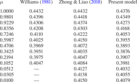
Table 3 displays the convergence of the Froude number at  $\bar {\mu } = 1.0053 \times 10^{-2}$, as predicted by the present scheme and by the model of Zhong & Liao (Reference Zhong and Liao2018). Incidentally, we observe that in the latter work, the parameter $\epsilon _{max}$ is an output of the scheme, and consequently it varies as the number of modes increases. The values of $\epsilon _{max}$ for the model of Zhong & Liao (Reference Zhong and Liao2018) are reported in the table caption. Conversely, in the present model, $\epsilon _{max}=0.4079$ for all the cases. Both the schemes prove to be in good agreement even when a relatively low number of modes is used.
Convergence of  $F$ for $\bar {\mu } = 1.0053 \times 10^{-2}$. We highlight that in Zhong & Liao (Reference Zhong and Liao2018), the parameter $\epsilon _{max}$ varies as the number of modes increases. Specifically, $\epsilon _{max} = 0.4134, 0.4141, 0.4145, 0.4148, 0.4150, 0.4150$. Conversely, in the present model, $\epsilon _{max}=0.4079$ in all the cases.

Figure 4(a) displays the free-surface solutions of maximum amplitude for  $\bar {\mu } = 4 {\rm \pi}$ (blue solid line), $\bar {\mu } = {\rm \pi}/4$ (red solid line) and $\bar {\mu } = {\rm \pi}/64$ (green solid line) scaled over one period (namely, $\ell _0 = 2 {\rm \pi}/\mu$), along with the theoretical slope ${\rm \pi} /3$ at the crests (dashed lines). In all the regimes of motion, the agreement with the theoretical slope is good, proving that the angle at the crest is $120^\circ$ as conjectured by Stokes (Reference Stokes1847). Incidentally, we highlight that the solutions obtained with the present scheme just approximate this theoretical angle since for $\nu > 0$, the derivative at the crest is always zero. This is shown in figure 4(b), where a detail of the deep-water case is displayed. Finally, figure 5 shows the solution in deep water (i.e. $\bar {\mu } = 4 {\rm \pi}$) along with the numerical results obtained in Dyachenko et al. (Reference Dyachenko, Lushnikov and Korotkevich2016) (green dots) and Schwartz (Reference Schwartz1974) (red diamonds) for waves in infinite depth. In comparison to these outputs, the present solution displays a small shift downwards along the vertical direction. In any case, the match with the outputs of Dyachenko et al. (Reference Dyachenko, Lushnikov and Korotkevich2016) and Schwartz (Reference Schwartz1974) appears good if the free surface is translated upwards (dashed line), proving that the solution with $\mu = {\rm \pi}/4$ is a good approximation of the solution for waves over infinite depth. Remarkably, the integral over the period of the translated solution gives $0.011$ against $-4.84 \times 10^{-4}$ of the original signal. This proves that (4.7) is satisfied accurately by the proposed iterative scheme, while the results by Dyachenko et al. (Reference Dyachenko, Lushnikov and Korotkevich2016) and Schwartz (Reference Schwartz1974) are actually characterized by a slight set-up.
(a) The maximum-amplitude free-surface solutions for  $\bar {\mu } = 4 {\rm \pi}$ (blue solid line), $\bar {\mu } = {\rm \pi}/4$ (red solid line) and $\bar {\mu } = {\rm \pi}/64$ (green solid line). (b) Detail of the solution for $\bar {\mu } = 4 {\rm \pi}$ (solid line). The dashed lines indicate the theoretical slope ${\rm \pi} /3$ at the crests.

The solution for  $\bar {\mu } = 4 {\rm \pi}$ (solid line) and the same signal with the addition of a set-up (dashed line) to match the results by Dyachenko et al. (Reference Dyachenko, Lushnikov and Korotkevich2016) (green dots) and Schwartz (Reference Schwartz1974) (red diamonds).

Before proceeding to the next section, we address some details about the numerical simulations. The most computationally expensive simulations are those characterized by the maximum wave amplitude in shallow-water conditions, since they require a large number of modes to satisfy the energy condition in (5.14). In particular, the simulation with  $\bar {\mu } = {\rm \pi}/512 = 6.1359 \times 10^{-3}$ (i.e. the shallowest case considered in the present work), $\epsilon _{max} = 0.4084$ and $60\,000$ modes reaches the convergence in $719$ iterations and takes about $800$ seconds with $42$ cores. Incidentally, we observe that in Zhong & Liao (Reference Zhong and Liao2018), the shallowest case was characterized by $\bar {\mu } = 1.0053 \times 10^{-2}$ and $50\,000$ modes, and a supercomputer was needed for the computations. This suggests that the present scheme can be regarded as a fast and accurate approximation of the singular solution (i.e. $\nu = 0$) described in Zhong & Liao (Reference Zhong and Liao2018). With respect to this, figure 6 displays the comparison with the shallowest case considered in Zhong & Liao (Reference Zhong and Liao2018), that is, $\bar {\mu } = 1.0053 \times 10^{-2}$. The solutions show overall good agreement (figure 6a), although the proposed iterative scheme slightly underestimates the crest height ( $\epsilon = 0.4085$ against $\epsilon = 0.4150$) and is characterized by a rounded peak instead of a sharp profile (figure 6b). Again, we underline that this behaviour is a consequence of the fact that the proposed model represents solutions with $\nu >0$ .
(a) The solution for  $\bar {\mu } = 1.0053 \times 10^{-2}$ as predicted by the homotopy analysis method in Zhong & Liao (Reference Zhong and Liao2018) (red solid lines) and by the present iterative method (black dashed lines). (b) Detail in a region close to the crest.

We highlight that the number of iterations to reach the convergence drastically reduces far from the conditions of maximum wave amplitude. For example, the shallowest case (i.e.  $\bar {\mu } = {\rm \pi}/512$), with $\epsilon = 0.35$ and $60\,000$ modes, reaches the convergence in $137$ iterations and takes about $102$ seconds with $42$ cores. Regardless, $8500$ modes are enough to satisfy the condition (5.14) on the energy. In this latter case, the convergence is reached in the same number of iterations and takes just $2.4$ seconds with $42$ cores, and $55.7$ seconds with a single core.
6.2. Comparisons with the existing theories
In this subsection, we consider highly nonlinear waves propagating in three different water regimes. Specifically, we set  $\epsilon = 0.35$ and choose $\bar {\mu } = {\rm \pi}/16$ (shallow-water regime), $\bar {\mu } = {\rm \pi}/4$ (intermediate-water regime) and $\bar {\mu } = {\rm \pi}$ (deep-water regime).
Figure 7 displays the evolution of the parameters  $F$,
$F$,  $B$,
$B$,  $\bar {Q}$ and $C_m$ as functions of the iterations. The rate of convergence is slower in the shallow-water limit, while it becomes faster as the depth increases (see the behaviour of $C_m$ in figure 7d). Generally, after a short transient, the parameters $F$,
$F$,  $B$ and $\bar {Q}$ reach a plateau and the subsequent iterations are necessary mainly for convergence of the highest modes of $\theta$. The overall distributions of the mode amplitudes $E_n$ at the convergence are displayed in figure 8. For all the cases, the amplitude of the highest modes is of order $10^{-15}$. Incidentally, we observe that the amplitudes are all positive.
Convergence of the solution for  $\epsilon = 0.35$ (fixed) and $\bar {\mu } = {\rm \pi}/16$ (red lines), $\bar {\mu } = {\rm \pi}/4$ (green lines) and $\bar {\mu } = {\rm \pi}$ (blues lines).

Amplitude  $E_n$ of the modes at the convergence for $\epsilon = 0.35$ (fixed) and $\bar {\mu } = {\rm \pi}/16$ (red line), $\bar {\mu } = {\rm \pi}/4$ (green line) and $\bar {\mu } = {\rm \pi}$ (blue line).

To better highlight the benefits of the proposed solution, we consider a comparison with fifth-order Stokes and cnoidal wave theories described in Fenton (Reference Fenton1985, Reference Fenton1979). Figure 9 displays the solutions for the free-surface elevation  $\eta$ as predicted by the present model and by the above-mentioned theories. For $\bar {\mu } = {\rm \pi}$ (deep water), figure 9(a) illustrates the comparison with the fifth-order Stokes solution (red dashed line). The overall match is very good, and the proposed solution practically coincides with the Stokes one. In this regime, the solution from the cnoidal wave theory is not available, since it is out of its range of validity. A comparison with both the theories is, to some extent, possible for $\bar {\mu } = {\rm \pi}/4$ (intermediate water, figure 9b). In this case, the fifth-order cnoidal wave (dash-dot green line) is close to that predicted by the present model (solid black line), except for a slight set-down. On the contrary, the Stokes solution shows non-physical oscillations caused by its second-order component. Finally, figure 9c displays the shallow-water case (namely, $\bar {\mu } = {\rm \pi}/16$). In this regime, the Stokes solution is out of its range of validity and therefore is not shown. On the contrary, the match between the present model and the cnoidal wave is very good, and the signals are practically overlapped.
Solutions for the free-surface elevation  $\eta$ for $\epsilon = 0.35$ (fixed) and (a) $\bar {\mu } = {\rm \pi}$, (b) $\bar {\mu } = {\rm \pi}/4$, and (c) $\bar {\mu } = {\rm \pi}/16$. The black solid lines indicate the proposed solution, the red dashed lines denote the firth-order Stokes solutions, and the green dash-dotted lines represent the fifth-order cnoidal theory solutions.

A more addressing example of the reliability of the proposed solution is obtained by comparing the solutions for  $F$ and $U_D$ with those predicted by the fifth-order Stokes and cnoidal wave theories. In particular, in figure 10, we consider three cases with decreasing values of $\epsilon$. For $\epsilon = 0.35$ (figures 10a,b), each of the above-mentioned theories gives results in fairly good agreement with the present model in its own range of applicability, but diverges rapidly out of it. The overall behaviour is confirmed for smaller values of $\epsilon$. Specifically, the match with the present model improves in deep water for the Stokes wave solution and in shallow water for the cnoidal wave one, but in intermediate water, their singularities are almost unaffected by the decrease of $\epsilon$. In this case, the most evident phenomenon is the shift of the singularities towards shallower depths caused by the decrease of the Ursell number. This behaviour is consistent with the bounds described in § 4.2 that predict the Stokes wave theory to hold true for $\hat {U}_r \ll 1$, and the cnoidal theory to be applicable for $\hat {U}_r > 1/4$.
Solutions for (a,c,e)  $F$ and (b,d, f) $U_D$, as predicted by the fifth-order theories for Stokes waves (red dashed lines; Fenton Reference Fenton1985) and cnoidal waves (green dash-dotted lines; Fenton Reference Fenton1979). The solid black lines are the outputs obtained through the proposed iterative scheme.

Summarizing, the proposed iterative model provides an accurate global solution all over the regimes of propagation and displays an overall good match with the fifth-order shallow- and deep-water theories in their respective regions of applicability.
6.3. An explicit formula for the wave celerity
The results described so far are obtained by assuming that the wavelength of the propagating wave is known. This allows for the evaluation of  $\bar {\mu }$ and consequently of all the related spatial scales described in §§ 2 and 3. Nonetheless, in practical applications, the wave period $T^*$ is generally known instead of the wavelength, therefore a way to deduce $\bar {\mu }$ from it is needed. The knowledge of an explicit expression for $F$ as a function of $\mu$ and $\epsilon$ is the key point to obtain $\bar {\mu }$ from the wave period. We start from the dispersion relation
 \begin{equation} c^* = \frac{\omega^*}{k_0^*} \quad \Rightarrow \quad \omega = \mu\,F(\mu, \epsilon ), \end{equation}
where  $\omega = \omega ^* t_0^*$ is the angular wave frequency, i.e. $\omega ^* = 2 {\rm \pi}/T^*$. Since $t_0^*$ depends on $z_0^*$ (and therefore on the wavelength), it is convenient to introduce the shallow-water scale $\bar {\omega } = \omega ^* \sqrt { h_0^*/g^*}$ and $\epsilon = \bar {\epsilon }\, H(\mu )$, so that (6.5) becomes
 \begin{equation} \bar{\omega} = \sqrt{\bar{\mu} \tanh(\bar{\mu})}\,F\left(\tanh(\bar{\mu}), \frac{\bar{\epsilon} \bar{\mu}}{\tanh(\bar{\mu})}\right). \end{equation}
Here,  $\bar {\epsilon }$ and $\bar {\omega }$ are known, while $\bar {\mu }$ has to be obtained by inversion. Since $1 \leq F \leq 1.3$ (the upper bound is attained for a solitary wave of maximum amplitude), the inversion can be performed by applying the bisection method over the segment $(\bar {\mu }_1,\bar {\mu }_2)$, where $\bar {\mu }_1 = (\bar {\omega }/1.3)^2$ and $\bar {\mu }_2 = ( \overline {\omega }^2 + \bar {\omega } \sqrt {\overline {\omega }^2 + 4} )/2$. For these bounds, we used the relations $\tanh (\bar {\mu }) \leq 1$ and $\tanh (\bar {\mu }) \geq \bar {\mu }/(1+\bar {\mu })$.
The final step is to provide an explicit expression for  $F$ as a function of $\mu$ and $\epsilon$. Since an explicit solution is not available, we provide a formula obtained through a regression analysis by using about 300 sample points in the $(\mu, \epsilon )$-plane. This reads
 \begin{equation} F( \mu, \epsilon ) = 1 + \epsilon^2 \left(\frac{a + b \mu + c \mu^2}{\epsilon + d \mu + e \mu^2}\right), \end{equation}
where
 \begin{equation} \left.\begin{gathered} a ={-}15.2479 \epsilon^3 + 10.9266 \epsilon^2 - 3.0256 \epsilon + 1.1712,\\ b = 26.9416 \epsilon^3 - 17.1964 \epsilon^2 + 5.6883 \epsilon - 2.2527,\\ c ={-}18.2407 \epsilon^3 + 11.7909 \epsilon^2 - 4.4316 \epsilon + 1.4138, \end{gathered}\right\} \end{equation}
and
 \begin{equation} \left.\begin{gathered} d = 141.0995 \epsilon^4 -119.6816 \epsilon^3 + 38.0355 \epsilon^2 -5.6719 \epsilon + 0.3527,\\ e ={-}119.3300 \epsilon^4 + 84.4075 \epsilon^3 - 19.0126 \epsilon^2 -0.0593 \epsilon + 0.3693. \end{gathered}\right\} \end{equation}
The structure of (6.7) is conceived to represent the asymptotic behaviours of  $F$ in deep- and shallow-water regimes. Specifically, $F = 1 + O(\epsilon )$ for $\mu \ll 1$ as predicted by the cnoidal wave theory (Fenton Reference Fenton1979), while $F = 1 + O(\epsilon ^2)$ for $\mu = O(1)$ as predicted by the Stokes theory (Fenton Reference Fenton1985).
Figure 11(a) displays the contour lines of (6.7) in the  $(\mu,\epsilon )$-plane. Specifically, the solution is drawn in the domain $(\mu, \epsilon ) \in [0,1] \times [0, \epsilon _{max}(\mu ) ]$, where $\epsilon _{max}$ is given by (6.1). The plot illustrates clearly the increase of the Froude number for increasing amplitudes and for smaller values of $\mu$. To verify the accuracy of the proposed formula, we consider the absolute relative errors with respect to the Stokes and cnoidal wave theories, that is,
 \begin{equation} \mathcal{E}_{stokes} = \left|1 - \frac{F_{stokes}}{F}\right|,\quad \mathcal{E}_{cnoidal} = \left|\, 1 - \frac{F_{cnoidal}}{F}\right|, \end{equation}
where  $F$ is computed using (6.7). These are displayed in figures 11(b,c), respectively. In both cases, the grey regions indicate the ranges where the above-mentioned theories are not applicable. Generally, the overall error maintains below $0.5\,\%$ in the largest part of the range of validity for both the theories, and increases slightly close to the upper bound of the domain (namely, for $\epsilon$ close to $\epsilon _{max}$), where it grows up to $1\,\%$ for the Stokes solution (figure 11b) and up to $2\,\%$ for the cnoidal wave solution (figure 11c). Incidentally, we highlight that in such a region, the accuracy of the fifth-order theories decreases rapidly, since $\epsilon \simeq 0.39$ and the truncation error becomes of order $\epsilon ^6 \simeq 3 \times 10^{-3}$.
Contours of (a) formula (6.7), and absolute relative errors with respect to (b) the Stokes wave theory (Fenton Reference Fenton1985) and (c) the cnoidal wave theory (Fenton Reference Fenton1979). The grey regions indicate the ranges where the above-mentioned theories are not applicable.

7. Conclusions
Starting from the integral equation of Byatt-Smith (Reference Byatt-Smith1970), we defined an iterative scheme to solve the problem of steady periodic waves propagating over a planar seabed. The proposed approach allowed for the modelling of the wave dynamics from deep- to shallow-water conditions, and up to the limit of maximum-amplitude waves.
The outputs of the iterative schemes were compared with the existing fifth-order theories in shallow- and deep-water conditions, and with the results (both theoretical and numerical) for maximum-amplitude waves available in the literature. In all cases, the proposed model displayed overall good agreement, proving to be reliable and accurate. Further, the proposed iterative scheme can be employed in practical applications concerning wave modelling and numerical benchmarking, thanks to its limited computational cost.
The global description of the wave dynamics over the different regimes of motion was possible through the definition of a new scaling capable of identifying the vertical length representative of the wave motion. This also allowed for a compact description and presentation of the results provided in this work.
Funding
The research activity has been developed within the Project Area ‘Applied Mathematics’ of the Department of Engineering, ICT and Technology for Energy and Transport (DIITET) of the Italian National Research Council (CNR). This work has been partially supported by the FUNBREAK-PRIN2017 project funded by the Italian Ministry MIUR under Grant Agreement no. 20172B7MY9_003.
Declaration of interests
The author reports no conflict of interest.
Appendix A. The convolution operator $\mathscr {C}$

In this appendix, we show the derivation of the convolution operator  $\mathscr {C}$ and recall briefly some useful theoretical results. We define the Fourier transform and its inverse as
 \begin{equation}
\mathscr{F}\left(f(x)\right)(y) = \int_\mathbb{R}
\overline{{\rm e}}^{iyx}\,f(x)\,\textrm{d}\,x,\quad
\mathscr{F}^{{-}1}\left(f(x)\right)(y) = \frac{1}{2 {\rm \pi}}
\int_\mathbb{R} {\rm e}^{{i}y
x}\,f(x)\,\textrm{d}\,x.
\end{equation}
\begin{equation}
\mathscr{F}\left(f(x)\right)(y) = \int_\mathbb{R}
\overline{{\rm e}}^{iyx}\,f(x)\,\textrm{d}\,x,\quad
\mathscr{F}^{{-}1}\left(f(x)\right)(y) = \frac{1}{2 {\rm \pi}}
\int_\mathbb{R} {\rm e}^{{i}y
x}\,f(x)\,\textrm{d}\,x.
\end{equation}Consequently, the following results hold true for convolution integrals:
 \begin{equation} \mathscr{F}(f * g) = \mathscr{F}(f)\mathscr{F}(g),\quad \mathscr{F}^{{-}1}(f * g) = 2{\rm \pi} \mathscr{F}^{{-}1}(f) \mathscr{F}^{{-}1}(g), \end{equation}
where the symbol  $*$ denotes the convolution operator. Now, let us consider the function
 \begin{equation} f(x) = \log\left(\left|\tanh\left( \alpha x \right)\right|\right) = \log\left(\tanh\left( \alpha | x | \right)\right), \end{equation}
where  $\alpha$ is a positive real constant. Differentiating this expression, we find
 \begin{equation} \dot{f}(x) = 2 \alpha\,\textrm{cosech}( 2 \alpha x ). \end{equation}
Then we multiply by  $x$ and apply the inverse Fourier transform, obtaining
 \begin{equation} \mathscr{F}^{{-}1}\left(x\,\dot{f}(x)\right)(y) = \frac{\gamma}{2}\, \textrm{sech}^2( \gamma y ), \end{equation}
where  $\gamma = {\rm \pi}/(4\alpha )$ and the result on the right-hand side is demonstrated in Appendix D of Sinolakis (Reference Sinolakis1986). Using the properties of the inverse Fourier transform, (A5) leads to the differential equation
 \begin{equation} y\,\frac{\textrm{d} \mathscr{F}^{{-}1}( f )}{\textrm{d} y} + \mathscr{F}^{{-}1}( f ) + \frac{\gamma}{2}\,\textrm{sech}^2( \gamma y ) = 0, \end{equation}
whose solution is
 \begin{equation} \mathscr{F}^{{-}1}( f )(y) ={-} \frac{\tanh( \gamma y )}{2y} + \frac{C_0}{y}, \end{equation}
where  $C_0$ is a constant. Since the inverse transform of a real even function is a real even function, the constant $C_0$ has to be zero. Then applying the Fourier transform and using (A5), we find, finally,
 \begin{equation} \mathscr{F}\left(\frac{\tanh( \gamma y )}{y}\right)(x) ={-}2 \log\left(\tanh\left(\frac{ {\rm \pi}| x |}{4 \gamma} \right)\right), \end{equation}
where  $\alpha = {\rm \pi}/(4\gamma )$ has been used. The above results also lead to the identities
 \begin{equation} \left.\begin{gathered} - 2 \int_{\mathbb{R}} \sin( \xi x ) \log\left(\tanh\left(\frac{ {\rm \pi}| x |}{4 \gamma}\right)\right) \textrm{d}\,x = 0, \\ - 2 \int_{\mathbb{R}} \cos( \xi x ) \log\left(\tanh\left(\frac{ {\rm \pi}| x |}{4 \gamma}\right)\right) \textrm{d}\,x = 2 {\rm \pi}\,\frac{\tanh( \gamma \xi )}{\xi}, \end{gathered}\right\} \end{equation}
where  $\xi \in \mathbb {R}$. Now we introduce the convolution operator
 \begin{equation} \mathscr{C}[f] = f(\,\cdot\,) * \left[-\frac{1}{\rm \pi} \log\left( \tanh\left(\frac{{\rm \pi}\,|\,\cdot\,|}{4 \gamma}\right)\right)\right]. \end{equation}
From the results obtained above, it immediately follows that
 \begin{equation} \mathscr{C}[{\rm e}^{{\rm i} \xi x}](y) = \frac{\tanh( \gamma \xi )}{\xi}\, {\rm e}^{{\rm i} \xi y}\quad \textrm{and} \quad \mathscr{C}[1](y) = \gamma. \end{equation}
Hence the definition of the inverse operator is straightforward:
 \begin{equation} \mathscr{C}^{{-}1}[{\rm e}^{{\rm i} \xi x}](y) = \frac{\xi}{\tanh\left( \gamma \xi \right)}\,{\rm e}^{{\rm i} \xi y}\quad \textrm{and} \quad \mathscr{C}^{{-}1}[1](y) = \frac{1}{\gamma}. \end{equation}
Note that, differently from  $\mathscr {C}$, the inverse operator cannot be represented as a convolution integral.
Appendix B. The analytical expression for $\eta _0$

Let us assume that  $\theta$ is a periodic even function with zero mean:
 \begin{equation} \theta = \sum_{n=1}^{\infty} E_n \cos\left( n \mu \varPhi \right)\quad \textrm{and} \quad \sum_{n=1}^{\infty} n \left| E_n \right| < \infty. \end{equation}
Then, applying the operator  $\mathscr {C}$ and its inverse, we immediately obtain
 \begin{equation} \mathscr{C}[\theta] = \sum_{n=1}^{\infty} \frac{\tanh(n \mu \varPsi_s)}{ n \mu }\,E_n \cos( n \mu \varPhi ),\quad \mathscr{C}^{{-}1}[\theta] = \sum_{n=1}^{\infty} \frac{n \mu E_n}{\tanh( n \mu \varPsi_s)} \cos( n \mu \varPhi ), \end{equation}
and consequently we find
 \begin{equation} \langle { \mathscr{C}[\theta] } \rangle = 0,\quad \langle { \mathscr{C}^{{-}1}[\theta] } \rangle = 0, \end{equation}
where the symbol  $\langle \,\cdot\, \rangle$ denotes the average over the wave period in the hodograph plane. More generally, we observe that for a generic periodic function $f$, the following relation holds true:
 \begin{equation} \langle { f } \rangle = 0 \quad \Leftrightarrow \quad \langle { \mathscr{C}[f] } \rangle = 0 \quad \Leftrightarrow \quad \langle { \mathscr{C}^{{-}1}[f] } \rangle = 0. \end{equation}
Now let us consider the condition (4.7). Applying the inverse operator  $\mathscr {C}^{-1}$ to (5.1), we obtain
 \begin{equation} \frac{\textrm{d}\,x_s}{\textrm{d} \varPhi} = 1 + \epsilon\,\mathscr{C}^{{-}1}[\theta]. \end{equation}
Then substituting in (4.7) and recalling that  $\langle {\theta } \rangle = 0$ and $\eta = \theta + \eta _0$, we obtain
 \begin{equation} \eta_0 ={-} \epsilon\,\langle {\theta\,\mathscr{C}^{{-}1}[\theta]} \rangle. \end{equation}
Finally, substituting the expression for  $\theta$, we find
 \begin{equation} \langle {\theta\,\mathscr{C}^{{-}1}[\theta] } \rangle = \sum_{n=1}^{\infty} \frac{n \mu }{\tanh(n \mu \varPsi_s)}\,\frac{E_n^2}{2} \geq 0. \end{equation}
This implies that  $\eta _0 \leq 0$, or equivalently, $\varPsi _s \leq H$.
Appendix C. Details on the convolution terms
Let us assume that that both  $\theta _m$ and $\varPsi _s^{(m)}$ are known, and that the solution for $\theta _m$ is expressed through a cosine series with $(N+1)$ modes (including $n=0$). This is written in the form
 \begin{equation} \theta_m = \sum_{|n| \leq N} e_n^{(m)} \exp\left( {\rm i} n \mu {\varPhi} \right),\quad \textrm{where}\ e_n^{(m)} = e_{{-}n}^{(m)} \textrm{ and } e_0^{(m)} = 0. \end{equation}
Accordingly, the coefficients of the cosine series in (A1a,b) are  $E_n^{(m)} = 2 e_n^{(m)}$ and $E_0^{(m)} = e_0^{(m)}$. It is simple to verify that all the terms in the iterative models are, in fact, represented by cosine series. As a consequence, it is sufficient to compute the modes for $0 \leq n \leq N$ and derive the remaining ones by symmetry. For non-negative values of $n$, the coefficients of the convolution terms are in the form of summations that span from the mode $p = n-N$ to the mode $p=N$. In particular, the term $S_m$ in (5.4) is given by
 \begin{equation} S_m = \sum_{|n| \leq N} s_n^{(m)} \exp\left( {\rm i} n \mu {\varPhi} \right), \quad \textrm{where}\ s_n^{(m)} = s_{{-}n}^{(m)}, \end{equation}
and the coefficients for  $n \geq 0$ are
 \begin{align} s_n^{(m)} = \mu^2 \sum_{p = n-N}^{N} p (n-p) \left[\frac{1}{\tanh\left(p \mu \varPsi_s^{(m)}\right) \tanh\left( (n-p) \mu \varPsi_s^{(m)}\right) } - 1\right] e_p^{(m)} e_{n-p}^{(m)}. \end{align}
Similarly, for  $\theta _m S_m$ we obtain
 \begin{equation} \theta_m S_m = \sum_{|n| \leq N} r_n^{(m)} \exp\left( {\rm i} n \mu {\varPhi} \right), \quad \textrm{where}\ r_n^{(m)} = r_{{-}n}^{(m)}, \end{equation}
and the coefficients for  $n \geq 0$ are
 \begin{equation} r_n^{(m)} = \frac{1}{2} \sum_{p = n-N}^{N} [s_p^{(m)} e_{n-p}^{(m)} + e_p^{(m)} s_{n-p}^{(m)}]. \end{equation}
In this latter case, a symmetric form has been used for the convolution. The last term to be computed is
 \begin{equation} \theta_m\,\mathscr{C}^{{-}1}[\theta_m] = \sum_{|n| \leq N} q_n^{(m)} \exp\left( {\rm i} n \mu {\varPhi} \right), \quad \textrm{where}\ q_n^{(m)} = q_{{-}n}^{(m)}, \end{equation}
whose coefficients (in symmetric form) for  $n \geq 0$ are
 \begin{equation} q_n^{(m)} = \frac{\mu}{2} \sum_{p = n-N}^{N} \left[\frac{p}{\tanh\left(p \mu \varPsi_s^{(m)}\right) } + \frac{n-p}{\tanh\left( (n-p) \mu \varPsi_s^{(m)}\right) }\right] e_p^{(m)} e_{n-p}^{(m)}. \end{equation}
After all the coefficients of the convolution integrals are computed, the evaluation of  $\chi _{m+1}$, $\beta _{m+1}$, $\theta _{m+1}$ and $\eta _0^{(m+1)}$ through (5.7), (5.8), (5.11) and (5.9) is straightforward. For example, $\left [\left [{S}\right ]\right ]$ and $\langle {S} \rangle$ are obtained immediately as
 \begin{equation} \left[\left[{S_m}\right]\right] = \sum_{|n| \leq N} s_n^{(m)} \left[1 - ({-}1)^n\right],\quad \langle {S_m} \rangle = s_0^{(m)}. \end{equation}
Appendix D. The analytical expressions for $z(\varPhi, \varPsi )$ and $x(\varPhi, \varPsi )$


Substituting (B5) in the integral expression (3.16), we obtain
 \begin{equation} z(\varPhi, \varPsi) ={-} H + \varPsi + \epsilon \int_{\mathbb{R}} \exp({-{\rm i} y \varPhi})\, \mathscr{F}^{{-}1}[\theta ]\, \frac{\sinh(y \varPsi ) }{\sinh(y \varPsi_s)}\,\textrm{d} y, \end{equation}
and, through the first equation in the system (3.14), we find
 \begin{equation} x(\varPhi, \varPsi) = x_0 + \varPhi + {\rm i}\epsilon \int_{\mathbb{R}} \exp({-{\rm i} y \varPhi})\, \mathscr{F}^{{-}1}[\theta ]\,\frac{\cosh(y \varPsi )}{\sinh(y \varPsi_s)}\,\textrm{d} y. \end{equation}
If  $\theta$ is given by the series (B1a,b), then we obtain
 $$\begin{gather} z(\varPhi, \varPsi) ={-} H + \varPsi + \epsilon \sum_{n=1}^{\infty} E_n\, \frac{\sinh(n \mu \varPsi) }{\sinh(n \mu \varPsi_s)} \cos( n \mu \varPhi ), \end{gather}$$
 $$\begin{gather}x(\varPhi, \varPsi) = x_0 + \varPhi + \epsilon \sum_{n=1}^{\infty} E_n\, \frac{\cosh(n \mu \varPsi) }{\sinh(n \mu \varPsi_s)}\sin( n \mu \varPhi ), \end{gather}$$
and finally,
 \begin{equation} x_s(\varPhi) = x(\varPhi, \varPsi_s) = x_0 + \varPhi + \epsilon \sum_{n=1}^{\infty} \frac{E_n }{\tanh(n \mu \varPsi_s)} \sin( n \mu \varPhi ). \end{equation}
The solution for the velocity field in the moving frame of reference is obtained from (3.10a,b) and reads
 \begin{equation} U = \left[\left(\frac{{\partial} x}{{\partial} \varPhi} \right)^2 + \left(\frac{{\partial} z}{{\partial} \varPhi} \right)^2\right]^{{-}1}\frac{{\partial} x}{{\partial} \varPhi},\quad W = \left[\left(\frac{{\partial} x}{{\partial} \varPhi} \right)^2 + \left(\frac{{\partial} z}{{\partial} \varPhi} \right)^2\right]^{{-}1}\frac{{\partial} z}{{\partial} \varPhi}. \end{equation}
Finally, using (3.15), we obtain the values at the free surface:
 \begin{equation} U_s = \left(\frac{F^2 + 2 \epsilon^2 B - 2 \epsilon \eta}{F^2}\right) \frac{\textrm{d}\,x_s}{\textrm{d} \varPhi},\quad W_s = \epsilon \left(\frac{F^2 + 2 \epsilon^2 B - 2 \epsilon \eta}{F^2}\right) \frac{\textrm{d} \eta}{\textrm{d} \varPhi}, \end{equation}
where  $\textrm {d} z_s/\textrm {d} \varPhi = \epsilon \, \textrm {d} \eta / \textrm {d} \varPhi$ has been used in the last equality.


 Open access