


1. Introduction
1.1. Unsteadiness and objectivity
Unsteadiness is a fundamental property of fluid flows and plays a critical role in turbulence and eddy formation, see Kolmogorov (Reference Kolmogorov1941) and Signell & Geyer (Reference Signell and Geyer1991). In Kolmogorov’s theory of turbulence, for instance, the dissipation of turbulent kinetic energy is related to unsteady velocity fluctuations. In addition to its fundamental conceptual importance, unsteady flows are of vital relevance in applied fluid mechanics, such as blood flow, see Ku (Reference Ku1997), wind farm turbulence, see Stevens & Meneveau (Reference Stevens and Meneveau2017), and aeroacoustics, see Howe (Reference Howe1998). Mathematically, the unsteady component of a velocity field $\boldsymbol{v}(\boldsymbol{x},t)$
is given by its partial time-derivative,
$\boldsymbol{v}(\boldsymbol{x},t)$
is given by its partial time-derivative,
 \begin{eqnarray} \frac {\partial \boldsymbol{v}}{\partial t}(\boldsymbol{x},t), \end{eqnarray}
which defines an Eulerian measure for its temporal variation at each point of the fluid domain. We emphasise the difference between the unsteady component and the material time derivative $\textrm{d}\boldsymbol{v}/\textrm{d}t$
, which measures the acceleration of an individual fluid particle and is generally non-zero even in steady flows. Since the perception of unsteadiness depends on the observer’s frame of reference, it is essential to consider how such quantities transform under changes of frame.
$\textrm{d}\boldsymbol{v}/\textrm{d}t$
, which measures the acceleration of an individual fluid particle and is generally non-zero even in steady flows. Since the perception of unsteadiness depends on the observer’s frame of reference, it is essential to consider how such quantities transform under changes of frame.
While fluid flows are frame-dependent, physical reasoning often supports the use of a special reference frame in which standard flow diagnostics become more meaningful. When such a reference frame can be defined, it is commonly referred to as the co-moving or proper frame of the fluid, see Landau & Lifshitz (Reference Landau and Lifshitz1975). Identifying proper frames is relatively straightforward when the flow exhibits an homogeneous direction of propagation, such as in periodic or infinite domains. This applies to phenomena like travelling waves or relative periodic orbits in shear flows, see Waleffe (Reference Waleffe2001), where a clearly defined base or mean velocity field can be determined. In some scenarios, even time-varying phase speeds can be computed, especially in channel flows, by minimising the discrepancy between the velocity field at position $x$
and
$x$
and $x-ct$
as demonstrated by Mellibovsky & Eckhardt (Reference Mellibovsky and Eckhardt2012) and Kreilos, Zammert & Eckhardt (Reference Kreilos, Zammert and Eckhardt2014). In general, however, unsteady flows have no preferred frame and are perceived differently by different observers.
$x-ct$
as demonstrated by Mellibovsky & Eckhardt (Reference Mellibovsky and Eckhardt2012) and Kreilos, Zammert & Eckhardt (Reference Kreilos, Zammert and Eckhardt2014). In general, however, unsteady flows have no preferred frame and are perceived differently by different observers.
Objectivity, or frame invariance, is a fundamental principle in continuum mechanics and fluid dynamics, ensuring that physical quantities and governing equations remain independent of an observer’s relative motion, see Truesdell & Noll (Reference Truesdell and Noll2004). Most quantities in fluid dynamics, such as the velocity field itself, vorticity, helicity and kinetic energy, however, are not objective: different observers will generally measure different values of these quantities, leading to discrepancies in data due to their frame dependence. The same applies to the unsteadiness of a velocity field: a general observer whose spatial location is defined by a Euclidean frame change will measure a different unsteadiness than the observer in the $\boldsymbol{x}$
frame. This problem is illustrated in figure 1, which shows multiple observers – unmanned aerial vehicles (UAVs) as used by Grabe, Bülthoff & Giordano (Reference Grabe, Bülthoff and Giordano2012) and Rhudy, Gu & Chao (Reference Rhudy, Gu and Chao2014) – measuring the velocity field of a coherent structure (tornado). We note that a frame change relative to the intended lab frame may also arise unintentionally from a source of pseudo-noise polluting the measurements, e.g. by unwanted oscillations introduced in the measurement set-up. As objectivity is broadly regarded as particularly crucial in vortex identification, see Lugt (Reference Lugt1979) and Haller (Reference Haller2005), we give a brief overview of Eulerian vortex detection and its relation to the unsteady component of the velocity field in the following subsection.
$\boldsymbol{x}$
frame. This problem is illustrated in figure 1, which shows multiple observers – unmanned aerial vehicles (UAVs) as used by Grabe, Bülthoff & Giordano (Reference Grabe, Bülthoff and Giordano2012) and Rhudy, Gu & Chao (Reference Rhudy, Gu and Chao2014) – measuring the velocity field of a coherent structure (tornado). We note that a frame change relative to the intended lab frame may also arise unintentionally from a source of pseudo-noise polluting the measurements, e.g. by unwanted oscillations introduced in the measurement set-up. As objectivity is broadly regarded as particularly crucial in vortex identification, see Lugt (Reference Lugt1979) and Haller (Reference Haller2005), we give a brief overview of Eulerian vortex detection and its relation to the unsteady component of the velocity field in the following subsection.
Sketch of multiple co-moving observers (UAVs) measuring a velocity field $\boldsymbol{v}$
of a coherent structure (tornado). Due to the frame dependence of
$\boldsymbol{v}$
of a coherent structure (tornado). Due to the frame dependence of $\boldsymbol{v}$
, each observer’s measurements of the velocity field will generally be different from the others’ and also different from the velocity field measured in the rest frame of the earth. These disagreements in the velocity field carry over to the partial time derivative
$\boldsymbol{v}$
, each observer’s measurements of the velocity field will generally be different from the others’ and also different from the velocity field measured in the rest frame of the earth. These disagreements in the velocity field carry over to the partial time derivative $\partial _t \boldsymbol{v}$
, the vorticity
$\partial _t \boldsymbol{v}$
, the vorticity $\boldsymbol{\nabla }\times \boldsymbol{v}$
and other quantities derived from
$\boldsymbol{\nabla }\times \boldsymbol{v}$
and other quantities derived from $\boldsymbol{v}$
.
$\boldsymbol{v}$
.

1.2. Objectivity, coherent structures and vortex detection
Eulerian vortex criteria date at least back to the seminal work of Okubo (Reference Okubo1970) and Weiss (Reference Weiss1991), who defined what is today known as the Okubo–Weiss (OW) criterion for two-dimensional flows. This definition was extended to three dimensions by Hunt, Wray & Moin (Reference Hunt, Wray and Moin1988) in what is today known as the $Q$
-criterion. Deficiencies of the
$Q$
-criterion. Deficiencies of the $Q$
-criterion in the analysis of three-dimensional steady and unsteady flows were illustrated and discussed in detail by Jeong & Hussain (Reference Jeong and Hussain1995), who also introduced the related
$Q$
-criterion in the analysis of three-dimensional steady and unsteady flows were illustrated and discussed in detail by Jeong & Hussain (Reference Jeong and Hussain1995), who also introduced the related $\lambda _2$
-criterion. Other Eulerian vortex criteria are the
$\lambda _2$
-criterion. Other Eulerian vortex criteria are the $\varDelta$
-criterion from Chong, Perry & Cantwell (Reference Chong, Perry and Cantwell1990) and the
$\varDelta$
-criterion from Chong, Perry & Cantwell (Reference Chong, Perry and Cantwell1990) and the $\lambda _{{ci}}$
of Chakraborty, Balachandar & Adrian (Reference Chakraborty, Balachandar and Adrian2005). Importantly, all of these criteria reduce to the OW criterion in the case of a two-dimensional velocity field as discussed by Pedergnana et al. (Reference Pedergnana, Oettinger, Langlois and Haller2020). As the vortex criteria OW,
$\lambda _{{ci}}$
of Chakraborty, Balachandar & Adrian (Reference Chakraborty, Balachandar and Adrian2005). Importantly, all of these criteria reduce to the OW criterion in the case of a two-dimensional velocity field as discussed by Pedergnana et al. (Reference Pedergnana, Oettinger, Langlois and Haller2020). As the vortex criteria OW, $Q$
,
$Q$
, $\varDelta$
,
$\varDelta$
, $\lambda _2$
and
$\lambda _2$
and $\lambda _{{ci}}$
all coincide for two-dimensional incompressible flows, they will be referred to here simply as the
$\lambda _{{ci}}$
all coincide for two-dimensional incompressible flows, they will be referred to here simply as the $Q$
-criterion in the context of planar, solenoidal velocity fields.
$Q$
-criterion in the context of planar, solenoidal velocity fields.
The inherent frame dependence of the most commonly used vortex criteria was noted by Haller (Reference Haller2005). For a recent review of various vortex criteria, we refer to Epps (Reference Epps2017), Zhang et al. (Reference Zhang, Qiu, Chen, Liu, Dong and Liu2018) and Günther & Theisel (Reference Günther and Theisel2018). Haller (Reference Haller2005) provided a two-dimensional, spatially linear example for which the $Q$
-criterion yields contradicting predictions on the nature of the flow depending on the frame in which the velocity field is presented. This result left open the question of whether the velocity field considered was physically meaningful and whether the same conclusions could be drawn in nonlinear fields as well. These points were addressed by Pedergnana et al. (Reference Pedergnana, Oettinger, Langlois and Haller2020), who demonstrated that the
$Q$
-criterion yields contradicting predictions on the nature of the flow depending on the frame in which the velocity field is presented. This result left open the question of whether the velocity field considered was physically meaningful and whether the same conclusions could be drawn in nonlinear fields as well. These points were addressed by Pedergnana et al. (Reference Pedergnana, Oettinger, Langlois and Haller2020), who demonstrated that the $Q$
-criterion yields false positive and false negative results for a class of exact, unsteady two-dimensional Navier–Stokes solutions which include the field originally proposed by Haller (Reference Haller2005). We note that this deficiency of the
$Q$
-criterion yields false positive and false negative results for a class of exact, unsteady two-dimensional Navier–Stokes solutions which include the field originally proposed by Haller (Reference Haller2005). We note that this deficiency of the $Q$
-criterion is fundamentally different from the issues discussed by Jeong & Hussain (Reference Jeong and Hussain1995), as it occurs specifically in unsteady velocity fields – in particular, steady fields who inherit a synthetic time dependence by transforming the velocity field to a rotating frame. When transforming back to the steady frame, the issues noted by Haller (Reference Haller2005) and Pedergnana et al. (Reference Pedergnana, Oettinger, Langlois and Haller2020) disappear. Therefore, in addition to its problems in identifying three-dimensional vortices, the above-mentioned criteria generally yield demonstrably inconsistent results in unsteady Navier–Stokes trial flows.
$Q$
-criterion is fundamentally different from the issues discussed by Jeong & Hussain (Reference Jeong and Hussain1995), as it occurs specifically in unsteady velocity fields – in particular, steady fields who inherit a synthetic time dependence by transforming the velocity field to a rotating frame. When transforming back to the steady frame, the issues noted by Haller (Reference Haller2005) and Pedergnana et al. (Reference Pedergnana, Oettinger, Langlois and Haller2020) disappear. Therefore, in addition to its problems in identifying three-dimensional vortices, the above-mentioned criteria generally yield demonstrably inconsistent results in unsteady Navier–Stokes trial flows.
Alternative approaches to vortex detection are based on Langrangian, i.e. particle motion-based methods and barrier methods, see Haller, Karrasch & Kogelbauer (Reference Haller, Karrasch and Kogelbauer2018, Reference Haller, Karrasch and Kogelbauer2020a , Haller et al. Reference Haller, Katsanoulis, Holzner, Frohnapfel and Gatti2020b ), Haller (Reference Haller2023). Such methods, however, are rather costly to evaluate, mathematically complex and sensitive to flow data features. Furthermore, barrier methods are difficult to benchmark since there are no classical analogues and are retrospective due to their inherent Lagrangian nature. Following a different line of research, several works have aimed to identify a minimally unsteady component of the velocity field, see Bujack, Hlawitschka & Joy (Reference Bujack, Hlawitschka and Joy2016), Günther et al. (Reference Günther, Gross and Theisel2017) and Kim & Günther (Reference Kim and Günther2019). In particular, Rojo & Günther (Reference Rojo and Günther2020) proposed a modified counterpart of the velocity field by switching to the steadiest reference frame of a given flow. To this end, a variational principle for the steadiest reference frame is defined from the partial time derivative of the velocity field in the changed frame, see also Matejka (Reference Matejka2002) for similar considerations in the context of weather systems. This approach was criticised by Haller (Reference Haller2021) and Kaszás et al. (Reference Kaszás, Pedergnana and Haller2023) because the obtained frame change is generally nonlinear, thus leading to local differences in how certain regions of the flow domain are pronounced, while Theisel et al. (Reference Theisel, Hadwiger, Rautek, Theußl and Günther2021) argue that vortex criteria can be objectivised by unsteadiness minimisation. This divide arises from the fact that the flow visualisation community uses a generalised notion of objectivity which allows also for nonlinear frame changes. This notion differs from the continuum mechanics viewpoint, where objectivity is defined as a passive transformation property under linear, Euclidean frame changes. The present work follows the latter philosophy, restricting the notion of objectivity to the definition of Truesdell & Noll (Reference Truesdell and Noll2004).
Another divide in the fluid dynamics community exists with regards to the definition of coherent structures, specifically between the philosophy of Hunt et al. (Reference Hunt, Wray and Moin1988) and Jeong & Hussain (Reference Jeong and Hussain1995), who define vortices as isosurfaces of Eulerian scalar quantities, and the view of Haller (Reference Haller2015), who defines coherent structures, including vortices, as a function of their Lagrangian fluid particle motion. A positive step towards overcoming this divide would be the definition of an Eulerian vortex criterion satisfying the objectivity requirements posed by Haller (Reference Haller2021) that does not exhibit any false positives or false negatives. The present work seeks to advance the field towards this direction by providing the first example of an objective vortex criterion that takes into account and – in part – corrects for the effect of an unsteady frame change.
1.3. Overview
Haller et al. (Reference Haller, Hadjighasem, Farazmand and Huhn2016) were the first to define an objective analogue of vorticity $\boldsymbol{\nabla }\times \boldsymbol{v}$
by subtracting its spatial mean. Their method was later extended to magnetic vortices by Rempel et al. (Reference Rempel, Gomes, Silva and Chian2019). A general programme to objectivise common Eulerian quantities such as vorticity, potential vorticity, helicity, linear momentum and energy was first proposed by Dauxois et al. (Reference Dauxois, Peacock, Bauer, Caulfield, Cenedese, Gorlé, Haller, Ivey, Linden, Meiburg, Pinardi, Vriend and Woods2019). The related question whether vortex criteria can be objectivised was raised by Haller (Reference Haller2021). Following the rationale of defining objective analogues of non-objective flow quantities, Kaszás et al. (Reference Kaszás, Pedergnana and Haller2023) recently proposed an objective analogue of the velocity field, the deformation velocity
$\boldsymbol{\nabla }\times \boldsymbol{v}$
by subtracting its spatial mean. Their method was later extended to magnetic vortices by Rempel et al. (Reference Rempel, Gomes, Silva and Chian2019). A general programme to objectivise common Eulerian quantities such as vorticity, potential vorticity, helicity, linear momentum and energy was first proposed by Dauxois et al. (Reference Dauxois, Peacock, Bauer, Caulfield, Cenedese, Gorlé, Haller, Ivey, Linden, Meiburg, Pinardi, Vriend and Woods2019). The related question whether vortex criteria can be objectivised was raised by Haller (Reference Haller2021). Following the rationale of defining objective analogues of non-objective flow quantities, Kaszás et al. (Reference Kaszás, Pedergnana and Haller2023) recently proposed an objective analogue of the velocity field, the deformation velocity $\boldsymbol{v}_{{d}}$
by subtracting the closest rigid-body motion approximation from the velocity field.
$\boldsymbol{v}_{{d}}$
by subtracting the closest rigid-body motion approximation from the velocity field.
The present research follows this general rationale by defining an objective analogue of the unsteady part of a velocity field. To this end, we first modify the time derivative of a general, unsteady velocity field by a frame change, the deformation unsteadiness $[\partial _t \boldsymbol{v}]_{{d}}$
, analogous to the objective deformation component of a velocity field derived by Kaszás et al. (Reference Kaszás, Pedergnana and Haller2023). While the deformation velocity is objective, we show that the deformation unsteadiness is, in general, not objective for an arbitrary frame change. We then present a variational principle based on the deformation unsteadiness and define a special reference frame through minimisation of a functional. At this special, optimal frame correction, we can prove that the deformation unsteadiness is objective and thus defines an objective analogue of the unsteadiness of a general velocity field. Furthermore, we use this special frame change to define an objective analogue of the classical
$[\partial _t \boldsymbol{v}]_{{d}}$
, analogous to the objective deformation component of a velocity field derived by Kaszás et al. (Reference Kaszás, Pedergnana and Haller2023). While the deformation velocity is objective, we show that the deformation unsteadiness is, in general, not objective for an arbitrary frame change. We then present a variational principle based on the deformation unsteadiness and define a special reference frame through minimisation of a functional. At this special, optimal frame correction, we can prove that the deformation unsteadiness is objective and thus defines an objective analogue of the unsteadiness of a general velocity field. Furthermore, we use this special frame change to define an objective analogue of the classical $Q$
-criterion introduced by Hunt et al. (Reference Hunt, Wray and Moin1988).
$Q$
-criterion introduced by Hunt et al. (Reference Hunt, Wray and Moin1988).
The paper is structured as follows. In § 2, we recall basic terminology and definitions related to the problem of objective observables from time-variate flow systems. In § 3, we define the deformation unsteadiness and a variational principle that seeks special frame changes that minimise the averaged deformation unsteadiness. Section 4 deals with the classical $Q$
-criterion and its objective analogue derived from unsteadiness minimisation. In § 5, we apply our methods to analytical flow examples, while in § 6, we consider simulated flow data. Section 7 gives a physical interpretation of the deformation unsteadiness and discusses limitations of our method, while § 8 presents conclusions and further perspectives.
$Q$
-criterion and its objective analogue derived from unsteadiness minimisation. In § 5, we apply our methods to analytical flow examples, while in § 6, we consider simulated flow data. Section 7 gives a physical interpretation of the deformation unsteadiness and discusses limitations of our method, while § 8 presents conclusions and further perspectives.
2. Preliminaries
Consider a general unsteady dynamical system
 \begin{equation} \dot {\boldsymbol{x}} = \boldsymbol{v}(\boldsymbol{x},t) \end{equation}
for $\boldsymbol{x}\in \mathcal{D}\subset \mathbb{R}^3$
, defined on a time-independent, connected domain
$\boldsymbol{x}\in \mathcal{D}\subset \mathbb{R}^3$
, defined on a time-independent, connected domain $\mathcal{D}$
and a sufficiently smooth, unsteady vector field
$\mathcal{D}$
and a sufficiently smooth, unsteady vector field $\boldsymbol{v}:\mathbb{R}^3\times [0,\infty )\to \mathbb{R}^3$
. For simplicity, we exclude unbounded domains or domains whose boundary changes with time, although these cases could be treated in a similar way. For any function
$\boldsymbol{v}:\mathbb{R}^3\times [0,\infty )\to \mathbb{R}^3$
. For simplicity, we exclude unbounded domains or domains whose boundary changes with time, although these cases could be treated in a similar way. For any function $f:\mathcal{D}\to \mathbb{R}$
, we define its spatial average as
$f:\mathcal{D}\to \mathbb{R}$
, we define its spatial average as
 \begin{equation} \overline {f}=\unicode{x2A0F}_{\mathcal{D}} f \,\textrm{d}V = \frac {1}{\mathrm{Vol}(\mathcal{D})}\int _{\mathcal{D}} f \,\textrm{d}V. \end{equation}
A general frame change is described by a one-parameter family of Euclidean transformations,
 \begin{equation} \boldsymbol{x}(t)= \unicode{x1D64C}(t)\boldsymbol{y}(t)+\boldsymbol{b}(t), \end{equation}
where $t\mapsto \unicode{x1D64C}(t)\in SO(3)$
is a smooth curve of orthogonal matrices and
$t\mapsto \unicode{x1D64C}(t)\in SO(3)$
is a smooth curve of orthogonal matrices and $t\mapsto \boldsymbol{b}(t)\in \mathbb{R}^3$
is a smooth curve of translation vectors. A quantity derived from a solution to (2.1) is called objective if it transforms neutrally under a general frame change of the form (2.3), see Truesdell & Noll (Reference Truesdell and Noll2004). More specifically, a scalar
$t\mapsto \boldsymbol{b}(t)\in \mathbb{R}^3$
is a smooth curve of translation vectors. A quantity derived from a solution to (2.1) is called objective if it transforms neutrally under a general frame change of the form (2.3), see Truesdell & Noll (Reference Truesdell and Noll2004). More specifically, a scalar $\alpha$
, vector
$\alpha$
, vector $\boldsymbol{a}$
or matrix
$\boldsymbol{a}$
or matrix $ \unicode{x1D63C}$
is called objective if it transforms according to
$ \unicode{x1D63C}$
is called objective if it transforms according to
 \begin{equation} \tilde {\alpha }(\boldsymbol{y},t)=\alpha (\boldsymbol{x},t) \quad \text{or} \quad \tilde {\boldsymbol{a}}(\boldsymbol{y},t)= \unicode{x1D64C}^T(t){\boldsymbol{a}}(\boldsymbol{x},t)\quad \text{or} \quad \tilde { \unicode{x1D63C}}(\boldsymbol{y},t)= \unicode{x1D64C}^T(t){ \unicode{x1D63C}}(\boldsymbol{x},t) \unicode{x1D64C}(t), \end{equation}
in the $\boldsymbol{y}$
-frame induced by (2.3). Recall that the velocity field itself is non-objective since it transforms according to
$\boldsymbol{y}$
-frame induced by (2.3). Recall that the velocity field itself is non-objective since it transforms according to
 \begin{equation} \tilde {\boldsymbol{v}}(\boldsymbol{y},t)= \unicode{x1D64C}^T(t)[{\boldsymbol{v}}(\boldsymbol{x},t)-\dot { \unicode{x1D64C}}(t)\boldsymbol{y}-\dot {\boldsymbol{b}}]. \end{equation}
Throughout the paper, we denote quantities in the transformed frame with a tilde. The coordinates in the transformed frame are denoted by $\boldsymbol{y}$
as defined in (2.3). For the subsequent calculations, we recall the one-to-one correspondence between skew-symmetric, three-by-three matrix
$\boldsymbol{y}$
as defined in (2.3). For the subsequent calculations, we recall the one-to-one correspondence between skew-symmetric, three-by-three matrix ${\varOmega }^T=-{\varOmega }$
and vectors
${\varOmega }^T=-{\varOmega }$
and vectors $\boldsymbol{\omega }\in \mathbb{R}^3$
by the relation
$\boldsymbol{\omega }\in \mathbb{R}^3$
by the relation
 \begin{equation} {\varOmega }\boldsymbol{a} = \boldsymbol{\omega } \times \boldsymbol{a} \end{equation}
for all $\boldsymbol{a}\in \mathbb{R}^3$
. Conversely, we write
$\boldsymbol{a}\in \mathbb{R}^3$
. Conversely, we write ${\varOmega } = \mathrm{mat}[\boldsymbol{\omega }]$
for the skew-symmetric matrix form of the vector
${\varOmega } = \mathrm{mat}[\boldsymbol{\omega }]$
for the skew-symmetric matrix form of the vector $\boldsymbol{\omega }$
that is uniquely defined by (2.6).
$\boldsymbol{\omega }$
that is uniquely defined by (2.6).
3. Objective unsteadiness minimisation
Unsteadiness minimisation was introduced by Rojo & Günther (Reference Rojo and Günther2020) by defining the functional
 \begin{equation} \mathcal{J}[ \unicode{x1D64C},\boldsymbol{b}]= \frac {1}{2} \int_{t_0}^{t_1} \unicode{x2A0F}_{\mathcal{D}} \left |\frac {\partial \tilde {\boldsymbol{v}}}{\partial t}(\boldsymbol{y},t)\right |^2 \,\textrm{d}V \,\textrm{d}t, \end{equation}
acting on frame changes, where $\tilde {\boldsymbol{v}}$
is the velocity field in the
$\tilde {\boldsymbol{v}}$
is the velocity field in the $\boldsymbol{y}$
-frame. As pointed out by Haller (Reference Haller2021), extremisers of (3.1) are generally not objective, see also the discussion by Theisel et al. (Reference Theisel, Hadwiger, Rautek, Theußl and Günther2021). In the following, we propose an alternative measure for the unsteady component of a velocity field. To this end, we will proceed in two steps. First, we define a frame-corrected version to the time-variate part of the velocity field. Then, we replace the partial time-derivative in the integrand of (3.1) with its frame-corrected analogue.
$\boldsymbol{y}$
-frame. As pointed out by Haller (Reference Haller2021), extremisers of (3.1) are generally not objective, see also the discussion by Theisel et al. (Reference Theisel, Hadwiger, Rautek, Theußl and Günther2021). In the following, we propose an alternative measure for the unsteady component of a velocity field. To this end, we will proceed in two steps. First, we define a frame-corrected version to the time-variate part of the velocity field. Then, we replace the partial time-derivative in the integrand of (3.1) with its frame-corrected analogue.
3.1. Deformation unsteadiness
Let us recall the definition of the deformation velocity $\boldsymbol{v}_{{d}}$
as introduced by Kaszás et al. (Reference Kaszás, Pedergnana and Haller2023),
$\boldsymbol{v}_{{d}}$
as introduced by Kaszás et al. (Reference Kaszás, Pedergnana and Haller2023),
 \begin{align} \boldsymbol{v}_{{d}}(\boldsymbol{x},t) & = \frac {\textrm{d}\boldsymbol{x}_{{d}}}{\textrm{d}t}-{\varOmega }_{\textit{RB}}(t)\boldsymbol{x}_{{d}}\nonumber\\ & =\boldsymbol{v}(\boldsymbol{x},t)-{{\varOmega }_{\textit{RB}}(t)\boldsymbol{x}_{{d}}-\overline {\boldsymbol{v}}(t)}, \end{align}
where $\boldsymbol{x}_{{d}}=\boldsymbol{x}-\overline {\boldsymbol{x}}$
is the deformation displacement and
$\boldsymbol{x}_{{d}}=\boldsymbol{x}-\overline {\boldsymbol{x}}$
is the deformation displacement and ${\varOmega }_{\textit{RB}}=-{\varOmega }_{\textit{RB}}^T$
is the skew-symmetric matrix accounting for the optimal rigid body correction. Indeed,
${\varOmega }_{\textit{RB}}=-{\varOmega }_{\textit{RB}}^T$
is the skew-symmetric matrix accounting for the optimal rigid body correction. Indeed, ${\varOmega }_{\textit{RB}}$
is obtained from minimising the
${\varOmega }_{\textit{RB}}$
is obtained from minimising the $L^2$
-distance between the velocity field and a rigid body motion. The deformation velocity field
$L^2$
-distance between the velocity field and a rigid body motion. The deformation velocity field $\boldsymbol{v}_{{d}}=\boldsymbol{v}-\boldsymbol{v}_{\textit{RB}}$
, for
$\boldsymbol{v}_{{d}}=\boldsymbol{v}-\boldsymbol{v}_{\textit{RB}}$
, for $\boldsymbol{v}_{\textit{RB}}={\varOmega }_{\textit{RB}}\boldsymbol{x}_{{d}}+\overline {\boldsymbol{v}}$
, describes the local difference between the velocity field
$\boldsymbol{v}_{\textit{RB}}={\varOmega }_{\textit{RB}}\boldsymbol{x}_{{d}}+\overline {\boldsymbol{v}}$
, describes the local difference between the velocity field $\boldsymbol{v}$
and the bulk rigid body motion of the flow domain. As shown by Kaszás et al. (Reference Kaszás, Pedergnana and Haller2023), the deformation velocity is, indeed, objective:
$\boldsymbol{v}$
and the bulk rigid body motion of the flow domain. As shown by Kaszás et al. (Reference Kaszás, Pedergnana and Haller2023), the deformation velocity is, indeed, objective: $\tilde {\boldsymbol{v}}_{{d}} = \unicode{x1D64C}^T\boldsymbol{v}_{{d}}$
. Their result is stated here for incompressible flows, but could be readily adapted to the compressible case using the formulae in the reference. In analogy to the deformation velocity (3.2), we define the deformation component of the time-derivative of
$\tilde {\boldsymbol{v}}_{{d}} = \unicode{x1D64C}^T\boldsymbol{v}_{{d}}$
. Their result is stated here for incompressible flows, but could be readily adapted to the compressible case using the formulae in the reference. In analogy to the deformation velocity (3.2), we define the deformation component of the time-derivative of $\boldsymbol{v}$
as
$\boldsymbol{v}$
as
 \begin{align} \bigg [\frac {\partial \boldsymbol{v}}{\partial t}\bigg ]_{{d}}(\boldsymbol{x},t) & = \frac {\partial \boldsymbol{v}_{{d}}(\boldsymbol{x},t)}{\partial t}-{\varOmega }_{\textit{US}}(t)\boldsymbol{v}_{{d}}(\boldsymbol{x},t)\nonumber\\ & = \frac {\partial \boldsymbol{v}(\boldsymbol{x},t)}{\partial t}-{\varOmega }_{\textit{US}}(t)\boldsymbol{v}_{{d}}(\boldsymbol{x},t)-\frac {\partial \boldsymbol{v}_{\textit{RB}}(\boldsymbol{x},t)}{\partial t}, \end{align}
for a time-dependent skew-symmetric matrix ${\varOmega }_{\textit{US}}$
, accounting for unsteadiness correction. Since (3.3) gives a material variant of the unsteady contribution of a general velocity field, we call
${\varOmega }_{\textit{US}}$
, accounting for unsteadiness correction. Since (3.3) gives a material variant of the unsteady contribution of a general velocity field, we call $[\partial \boldsymbol{v}/\partial t]_{{d}}$
deformation unsteadiness. The deformation unsteadiness
$[\partial \boldsymbol{v}/\partial t]_{{d}}$
deformation unsteadiness. The deformation unsteadiness $[\partial \boldsymbol{v}/\partial t]_{{d}}$
describes the instantaneous local rate of change of the fluid with respect to a fictitious bulk rigid body acceleration of the problem domain. We stress at this point that
$[\partial \boldsymbol{v}/\partial t]_{{d}}$
describes the instantaneous local rate of change of the fluid with respect to a fictitious bulk rigid body acceleration of the problem domain. We stress at this point that $[\partial \boldsymbol{v}/\partial t]_{{d}}$
in itself is not an objective analogue of the acceleration
$[\partial \boldsymbol{v}/\partial t]_{{d}}$
in itself is not an objective analogue of the acceleration $\boldsymbol{a}=\textrm{d}\boldsymbol{v}/\textrm{d}t$
, but much rather a frame-corrected version of the partial time-derivative
$\boldsymbol{a}=\textrm{d}\boldsymbol{v}/\textrm{d}t$
, but much rather a frame-corrected version of the partial time-derivative $\partial \boldsymbol{v}/\partial t$
. A more detailed physical interpretation of the deformation unsteadiness is given in § 7.
$\partial \boldsymbol{v}/\partial t$
. A more detailed physical interpretation of the deformation unsteadiness is given in § 7.
We further stress that the deformation unsteadiness is, other than the deformation velocity $\boldsymbol{v}_{{d}}$
, not objective for an arbitrary skew-symmetric matrix
$\boldsymbol{v}_{{d}}$
, not objective for an arbitrary skew-symmetric matrix ${\varOmega }_{\textit{US}}$
. Indeed, for
${\varOmega }_{\textit{US}}$
. Indeed, for $[\partial \boldsymbol{v}/\partial t]_{{d}}$
to be objective,
$[\partial \boldsymbol{v}/\partial t]_{{d}}$
to be objective, ${\varOmega }_{\textit{US}}$
must transform like a spin tensor, see Truesdell & Noll (Reference Truesdell and Noll2004). Recall that a two-dimensional matrix
${\varOmega }_{\textit{US}}$
must transform like a spin tensor, see Truesdell & Noll (Reference Truesdell and Noll2004). Recall that a two-dimensional matrix $\varOmega$
transforms as a spin tensor under the Euclidean transformations (2.3) if
$\varOmega$
transforms as a spin tensor under the Euclidean transformations (2.3) if
 \begin{equation} \widetilde {{\varOmega }} = \unicode{x1D64C}^T{{\varOmega }} \unicode{x1D64C}- \unicode{x1D64C}^T\dot { \unicode{x1D64C}}. \end{equation}
Indeed, assuming the transformation property (3.4) for ${\varOmega }_{\textit{US}}$
, a direct calculation shows that
${\varOmega }_{\textit{US}}$
, a direct calculation shows that
 \begin{align} \bigg [\widetilde {\frac {\partial \boldsymbol{v}}{\partial t}}\bigg ]_{{d}} & = \unicode{x1D64C}^T\frac {\partial \boldsymbol{v}_{{d}}}{\partial t}+\dot { \unicode{x1D64C}}^T\boldsymbol{v}_{{d}}-\tilde {{\varOmega }}_{\textit{US}} \unicode{x1D64C}^T\boldsymbol{v}_{{d}}\nonumber\\ & = \unicode{x1D64C}^T\frac {\partial \boldsymbol{v}_{{d}}}{\partial t}+\dot { \unicode{x1D64C}}^T\boldsymbol{v}_{{d}}- \unicode{x1D64C}^T{\varOmega }_{\textit{US}}\boldsymbol{v}_{{d}} {+} \unicode{x1D64C}^T\dot { \unicode{x1D64C}} \unicode{x1D64C}^T\boldsymbol{v}_{{d}}\nonumber\\ & = \unicode{x1D64C}^T\frac {\partial \boldsymbol{v}_{{d}}}{\partial t}- \unicode{x1D64C}^T{\varOmega }_{\textit{US}}{\boldsymbol{v}_{{d}}}, \end{align}
where we used $\widetilde {\boldsymbol{v}}_{{d}}= \unicode{x1D64C}^T \boldsymbol{v}_{{d}}$
and the property that
$\widetilde {\boldsymbol{v}}_{{d}}= \unicode{x1D64C}^T \boldsymbol{v}_{{d}}$
and the property that $\dot { \unicode{x1D64C}} = - \unicode{x1D64C}\dot { \unicode{x1D64C}}^T \unicode{x1D64C}$
for the time derivative of rotation matrices.
$\dot { \unicode{x1D64C}} = - \unicode{x1D64C}\dot { \unicode{x1D64C}}^T \unicode{x1D64C}$
for the time derivative of rotation matrices.
We thus seek a special reference frame ${\varOmega }_{\textit{US}}$
that transforms as a spin tensor to make the deformation unsteadiness objective. In the following, we define a measure of the unsteadiness based on the spatio-temporal mean of (3.3) to single out an optimal unsteadiness correction
${\varOmega }_{\textit{US}}$
that transforms as a spin tensor to make the deformation unsteadiness objective. In the following, we define a measure of the unsteadiness based on the spatio-temporal mean of (3.3) to single out an optimal unsteadiness correction ${\varOmega }_{\textit{US}}$
and prove that this frame change transforms as (3.4).
${\varOmega }_{\textit{US}}$
and prove that this frame change transforms as (3.4).
3.2. Objective unsteadiness minimisation
We define the objective equivalent of the unsteadiness action by replacing $\partial \tilde {\boldsymbol{v}}/\partial t$
in (3.1) by the deformation unsteadiness
$\partial \tilde {\boldsymbol{v}}/\partial t$
in (3.1) by the deformation unsteadiness $ [\partial \boldsymbol{v}/\partial t]_{{d}}$
to obtain the functional
$ [\partial \boldsymbol{v}/\partial t]_{{d}}$
to obtain the functional
 \begin{equation} \mathcal{S}[{\varOmega }_{\textit{RB}},{\varOmega }_{\textit{US}}]= \frac {1}{2} \int _{t_0}^{t_1} \unicode{x2A0F}_{\mathcal{D}} \left |\left [\frac {\partial \boldsymbol{v}}{\partial t}\right ]_{{d}}(\boldsymbol{x},t;{\varOmega }_{\textit{RB}},\dot {{\varOmega }}_{\textit{RB}},{\varOmega }_{\textit{US}})\right |^2 \,\textrm{d}V \,\textrm{d}t. \end{equation}
We remark that the optimisation of (3.6) could be carried out for the rigid body frame change ${\varOmega }_{\textit{RB}}$
and the unsteadiness frame change
${\varOmega }_{\textit{RB}}$
and the unsteadiness frame change ${\varOmega }_{\textit{US}}$
simultaneously. In the following, however, we assume that the rigid body frame change that defines the deformation velocity is fixed and optimise for the unsteadiness frame change alone. Indeed, for fixed deformation velocity
${\varOmega }_{\textit{US}}$
simultaneously. In the following, however, we assume that the rigid body frame change that defines the deformation velocity is fixed and optimise for the unsteadiness frame change alone. Indeed, for fixed deformation velocity $\boldsymbol{v}_{{d}}$
, i.e. for fixed
$\boldsymbol{v}_{{d}}$
, i.e. for fixed ${\varOmega }_{\textit{RB}}$
, the functional (3.6) is convex with respect to
${\varOmega }_{\textit{RB}}$
, the functional (3.6) is convex with respect to ${\varOmega }_{\textit{US}}$
, thus guaranteeing that extremisers will be minimisers.
${\varOmega }_{\textit{US}}$
, thus guaranteeing that extremisers will be minimisers.
The partial variation with respect to unsteadiness rotation can be easily calculated by
 \begin{equation} \frac {\delta \mathcal{S}}{\delta {\varOmega }_{\textit{US}}} = \overline {\boldsymbol{v}_{{d}}\times ({\varOmega }_{\textit{US}}\boldsymbol{v}_{{d}}-\partial _t\boldsymbol{v}_{{d}})}, \end{equation}
see Appendix A for an explicit step-by-step derivation. Using properties of the cross-product, the Euler–Lagrange equation $\delta \mathcal{S}/\delta {\varOmega }_{\textit{US}} = 0$
can be rewritten as
$\delta \mathcal{S}/\delta {\varOmega }_{\textit{US}} = 0$
can be rewritten as
 \begin{equation} (\overline {|\boldsymbol{v}_{{d}}|^2} \unicode{x1D644}-\overline {\boldsymbol{v}_{{d}}{\otimes } \boldsymbol{v}_{{d}}} )\boldsymbol{\omega }_{\textit{US}} -\overline {\boldsymbol{v}_{{d}}\times \partial _t\boldsymbol{v}_{{d}}}=0, \end{equation}
where ${\varOmega }_{\textit{US}} = \mathrm{mat}[\boldsymbol{\omega }_{\textit{US}}]$
is the skew-symmetric matrix form of
${\varOmega }_{\textit{US}} = \mathrm{mat}[\boldsymbol{\omega }_{\textit{US}}]$
is the skew-symmetric matrix form of $\boldsymbol{\omega }_{\textit{US}}$
. In turn, (3.8) can be solved explicitly by
$\boldsymbol{\omega }_{\textit{US}}$
. In turn, (3.8) can be solved explicitly by
 \begin{equation} \boldsymbol{\omega }_{\textit{US}} = {\varTheta }_v^{-1} \overline {\boldsymbol{v}_{{d}}\times \partial _t\boldsymbol{v}_{{d}}}, \end{equation}
where we define the moment of inertia tensor associated to the deformation velocity defined as
 \begin{equation} {\varTheta }_v = \overline {|\boldsymbol{v}_{{d}}|^2} \unicode{x1D644} - \overline {(\boldsymbol{v}_{{d}}\otimes \boldsymbol{v}_{{d}})}, \end{equation}
which is invertible for a general deformation velocity. The skew-symmetric matrix defined by (3.9) gives the optimal correction to the unsteady component of a velocity field. An elementary calculation shows that ${\varOmega }_{\textit{US}}$
, indeed, transforms as a spin tensor, see Appendix B, and the deformation unsteadiness at the optimal frame change thus becomes objective, see (3.5).
${\varOmega }_{\textit{US}}$
, indeed, transforms as a spin tensor, see Appendix B, and the deformation unsteadiness at the optimal frame change thus becomes objective, see (3.5).
Remark 1.
Our line of reasoning deviates from the classical rationale of groups acting on functionals. A general principle in the calculus of variations states that if a functional is invariant by a smooth group action, so is its first variation, see Giaquinta & Hildebrandt (
Reference Giaquinta and Hildebrandt2013
). The group of Euclidean transforms acts on the deformation unsteadiness functional (3.6) through frame changes (2.3), but does not leave its integrand, the deformation unsteadiness, invariant for a general ${\varOmega }_{\textit{US}}$
. Much rather, as outlined in (3.5), the deformation unsteadiness functional is only invariant at those skew-symmetric matrices which transform as a spin tensor. Only at the extremiser, the integrand is invariant under the full group action.
${\varOmega }_{\textit{US}}$
. Much rather, as outlined in (3.5), the deformation unsteadiness functional is only invariant at those skew-symmetric matrices which transform as a spin tensor. Only at the extremiser, the integrand is invariant under the full group action.
Remark 2.
Instead of assuming the deformation velocity $\boldsymbol{v}_{{d}}$
as fixed in the objective unsteadiness minimisation performed in §
3.2
, i.e. assuming
$\boldsymbol{v}_{{d}}$
as fixed in the objective unsteadiness minimisation performed in §
3.2
, i.e. assuming ${\varOmega }_{\textrm {RB}}$
to be given, one may vary
${\varOmega }_{\textrm {RB}}$
to be given, one may vary ${\varOmega }_{\textrm {RB}}$
and
${\varOmega }_{\textrm {RB}}$
and ${\varOmega }_{\textit{US}}$
both to obtain a further decrease of the averaged deformation velocity. While this more general approach allows for a more immediate physical interpretation, the resulting Euler–Lagrange equations are nonlinear, second-order in time differential equations in the unknowns and, thus, cannot be solved in closed form.
${\varOmega }_{\textit{US}}$
both to obtain a further decrease of the averaged deformation velocity. While this more general approach allows for a more immediate physical interpretation, the resulting Euler–Lagrange equations are nonlinear, second-order in time differential equations in the unknowns and, thus, cannot be solved in closed form.
4. An objective $Q$
-criterion for unsteady flows
$Q$
-criterion for unsteady flows

In this section, we use the special frame change ${\varOmega }_{\textit{US}}$
obtained by minimising (3.6) to define a modified version of a vortex detection criterion. The classical
${\varOmega }_{\textit{US}}$
obtained by minimising (3.6) to define a modified version of a vortex detection criterion. The classical $Q$
-criterion, as defined by Okubo (Reference Okubo1970), Weiss (Reference Weiss1991) and Hunt et al. (Reference Hunt, Wray and Moin1988), compares the magnitude of the symmetric part of
$Q$
-criterion, as defined by Okubo (Reference Okubo1970), Weiss (Reference Weiss1991) and Hunt et al. (Reference Hunt, Wray and Moin1988), compares the magnitude of the symmetric part of $\boldsymbol{\nabla } \boldsymbol{v}$
with its anti-symmetric part,
$\boldsymbol{\nabla } \boldsymbol{v}$
with its anti-symmetric part,
 \begin{equation} Q = \frac {1}{2}\big (\|{ \unicode{x1D652}}\left(\boldsymbol{x},t\right)\|^2-\| \unicode{x1D64E}(\boldsymbol{x},t)\|^2\big), \end{equation}
where $ \unicode{x1D64E} = 1/2[ \boldsymbol{\nabla } \boldsymbol{v} + (\boldsymbol{\nabla } \boldsymbol{v})^T]$
is the strain-rate tensor and
$ \unicode{x1D64E} = 1/2[ \boldsymbol{\nabla } \boldsymbol{v} + (\boldsymbol{\nabla } \boldsymbol{v})^T]$
is the strain-rate tensor and ${ \unicode{x1D652}}= 1/2[ \boldsymbol{\nabla } \boldsymbol{v}- (\boldsymbol{\nabla } \boldsymbol{v})^T]$
is the spin tensor. According to the
${ \unicode{x1D652}}= 1/2[ \boldsymbol{\nabla } \boldsymbol{v}- (\boldsymbol{\nabla } \boldsymbol{v})^T]$
is the spin tensor. According to the $Q$
-criterion, a vortex is a region where the rotation-related motion dominates the stretch-related motion, i.e. where
$Q$
-criterion, a vortex is a region where the rotation-related motion dominates the stretch-related motion, i.e. where $Q$
is positive.
$Q$
is positive.
Although the $Q$
-criterion (4.1) is a widely used Eulerian method for vortex identification based on the local balance between vorticity and strain, one issue with the
$Q$
-criterion (4.1) is a widely used Eulerian method for vortex identification based on the local balance between vorticity and strain, one issue with the $Q$
-criterion is its lack of objectivity. This can lead to inconsistent or misleading vortex detection, especially in geophysical or engineering applications where the flow is observed from different frames. Furthermore, the criterion is purely instantaneous and local, meaning it does not account for the material coherence or long-term behaviour of fluid elements, often identifying spurious or non-persistent vortical structures. These limitations have been extensively discussed by Haller (Reference Haller2005).
$Q$
-criterion is its lack of objectivity. This can lead to inconsistent or misleading vortex detection, especially in geophysical or engineering applications where the flow is observed from different frames. Furthermore, the criterion is purely instantaneous and local, meaning it does not account for the material coherence or long-term behaviour of fluid elements, often identifying spurious or non-persistent vortical structures. These limitations have been extensively discussed by Haller (Reference Haller2005).
In an attempt to remedy these deficiencies, we define an objective version of (4.1) by replacing the velocity field $\boldsymbol{v}$
with
$\boldsymbol{v}$
with $\boldsymbol{v}_{{d,\textit{US}}}=\boldsymbol{v}-\boldsymbol{v}_{\textit{US}}$
, where
$\boldsymbol{v}_{{d,\textit{US}}}=\boldsymbol{v}-\boldsymbol{v}_{\textit{US}}$
, where
 \begin{equation} \boldsymbol{v}_{\textit{US}}={\varOmega }_{\textit{US}} (\boldsymbol{x}-\overline {\boldsymbol{x}}) +\overline {\boldsymbol{v}}, \end{equation}
in analogy to the deformation velocity field (3.2),
 \begin{equation} Q_{\textit{US}}=\frac {1}{2}\big(\|{ \unicode{x1D652}}(\boldsymbol{x},t)-{\varOmega }_{\textit{US}}(t)\|^2-\| \unicode{x1D64E}(\boldsymbol{x},t)\|^2\big) , \end{equation}
where ${\varOmega }_{\textit{US}}$
is derived as a critical point of (3.6). Since
${\varOmega }_{\textit{US}}$
is derived as a critical point of (3.6). Since ${\varOmega }_{\textit{US}}$
transforms like a spin tensor, see (3.4), the difference between
${\varOmega }_{\textit{US}}$
transforms like a spin tensor, see (3.4), the difference between $W$
and
$W$
and ${\varOmega }_{\textit{US}}$
appearing in (4.3) is objective. Consequently, by the objectivity of the strain-rate tensor
${\varOmega }_{\textit{US}}$
appearing in (4.3) is objective. Consequently, by the objectivity of the strain-rate tensor $S$
,
$S$
, $Q_{\textit{US}}$
is an objective scalar. Another objective version of the
$Q_{\textit{US}}$
is an objective scalar. Another objective version of the $Q$
-criterion,
$Q$
-criterion, $Q_{\textit{RB}}$
, first defined by Kaszás et al. (Reference Kaszás, Pedergnana and Haller2023), can be obtained by replacing
$Q_{\textit{RB}}$
, first defined by Kaszás et al. (Reference Kaszás, Pedergnana and Haller2023), can be obtained by replacing ${\varOmega }_{\textit{US}}$
with
${\varOmega }_{\textit{US}}$
with ${\varOmega }_{\textit{RB}}$
in (4.3).
${\varOmega }_{\textit{RB}}$
in (4.3).
5. Analytical examples and applications to vortex detection
In this section, we apply the deformation unsteadiness to several examples, including analytical flow fields as well as simulated flow data. In § 5.1, we consider a linear solution to the Navier–Stokes equation whose perceived unsteadiness is entirely due to an unsteady frame change. In § 5.2, we analyse an analytic two-dimensional flow field with separation and reattachment. Section 5.3 deals with an unsteady, quadratic Navier–Stokes field whose vortical structure can be deduced from $\boldsymbol{v}_{\textit{US}}$
, while § 5.4 applies the deformation unsteadiness to vortex detection for the analytic linear flow field of § 5.1. A pseudocode detailing the steps involved in the computation of
$\boldsymbol{v}_{\textit{US}}$
, while § 5.4 applies the deformation unsteadiness to vortex detection for the analytic linear flow field of § 5.1. A pseudocode detailing the steps involved in the computation of $[\partial _t \boldsymbol{v}]_{{d}}$
is provided in Appendix C.
$[\partial _t \boldsymbol{v}]_{{d}}$
is provided in Appendix C.
5.1. Spatially linear field in unsteady frame
Consider the linear velocity field
 \begin{eqnarray} \boldsymbol{v}(\boldsymbol{x},t)= \unicode{x1D63C}(t)\boldsymbol{x}, \end{eqnarray}
with the time-dependent matrix $ \unicode{x1D63C}$
given by
$ \unicode{x1D63C}$
given by
 \begin{eqnarray} \unicode{x1D63C}(t)= \begin{pmatrix} -\sin (Ct) & \cos (Ct) - \dfrac {{\omega }}{2} & 0 \\ \cos (Ct) + \dfrac {{\omega }}{2} & \sin (Ct) & 0 \\ 0 & 0 & 0 \end{pmatrix} \end{eqnarray}
for $C$
,
$C$
, $\omega \in \mathbb{R}$
over a cubic (square) domain
$\omega \in \mathbb{R}$
over a cubic (square) domain $[-L/2,L/2]\times [-L/2,L/2]\times [-L/2,L/2]$
. As illustrated by Pedergnana et al. (Reference Pedergnana, Oettinger, Langlois and Haller2020), the unsteadiness of this velocity field derives solely from an unsteady frame change, which is applied to a steady velocity field to yield the unsteady field (5.1). This field is thus intrinsically steady in the sense that its unsteadiness can be eliminated by an observer in a suitable frame.
$[-L/2,L/2]\times [-L/2,L/2]\times [-L/2,L/2]$
. As illustrated by Pedergnana et al. (Reference Pedergnana, Oettinger, Langlois and Haller2020), the unsteadiness of this velocity field derives solely from an unsteady frame change, which is applied to a steady velocity field to yield the unsteady field (5.1). This field is thus intrinsically steady in the sense that its unsteadiness can be eliminated by an observer in a suitable frame.
Remarkably, these observations, which date back to the work of Haller (Reference Haller2005), are supported by the analysis in this work. Indeed, the deformation unsteadiness, given by (3.3), computed for the field (5.1), vanishes identically. For completeness, the derivation of this result is given in Appendix D. Due to the objectivity of the deformation unsteadiness at the extremiser, this result holds for any observer. Therefore, the deformation unsteadiness derived in this work correctly judges the unsteady velocity field (5.1) as inherently steady.
5.2. Separation and reattachment flow
Consider the classical kinematic example of Lekien & Haller (Reference Lekien and Haller2008) given by the unsteady stream function
 \begin{eqnarray} \psi (\boldsymbol{x}, t) = \big ( |\boldsymbol{x}|^2 - 1 \big )\bigl ( x_1 \sin (\omega _s t) + x_2 \cos (\omega _s t) \bigr ) - \frac {1}{2}\,\omega _s |\boldsymbol{x}|^2 \end{eqnarray}
for a general frequency $\omega _s\in \mathbb{R}$
, defined on the unit circle. The flow derived from (5.3) exhibits coexisting fluid separation and reattachment. In the following, we set
$\omega _s\in \mathbb{R}$
, defined on the unit circle. The flow derived from (5.3) exhibits coexisting fluid separation and reattachment. In the following, we set $\omega _s=1$
and consider the flow field at the time
$\omega _s=1$
and consider the flow field at the time $t=0.5$
. Figure 2(a) depicts isocontours of the norm of the partial time-derivative, which can be calculated as
$t=0.5$
. Figure 2(a) depicts isocontours of the norm of the partial time-derivative, which can be calculated as
 \begin{align} \frac {\partial \boldsymbol{v}}{\partial t}(\boldsymbol{x},t)=\begin{pmatrix} -2x_2 \bigl (\omega _s x_2 \sin (t \omega _s) - \omega _s x_1 \cos (t \omega _s)\bigr ) - \omega _s \sin (t \omega _s)\,(|\boldsymbol{x}|^2 - 1) \\[1em] \;\;2x_1 \bigl (\omega _s x_2 \sin (t \omega _s) - \omega _s x_1 \cos (t \omega _s)\bigr ) - \omega _s \cos (t \omega _s)\,(|\boldsymbol{x}|^2 - 1) \end{pmatrix}\!. \end{align}
Isocontours of the norms of (a) the partial time derivative and (b) the deformation unsteadiness for the two-dimensional unsteady flow field described by the stream function (5.3). The coexistence of two diametrically opposed flow cells is revealed only by the objective deformation unsteadiness, but not by the non-objective partial time derivative. In panel (b), the zero contour of the deformation unsteadiness is coloured in red.

The deformation unsteadiness for this flow takes the explicit form
 \begin{align} \left [\frac {\partial \boldsymbol{v}}{\partial t}\right ]_{{d}}(\boldsymbol{x},t)=\begin{pmatrix} \dfrac {-\omega _s x_1 \bigl (x_2 \cos (t \omega _s) + x_1 \sin (t \omega _s)\bigr ) \bigl (|\boldsymbol{x}|^2 - 1\bigr )}{|\boldsymbol{x}|^2} \\[1em] \dfrac {-\omega _s x_2 \bigl (x_2 \cos (t \omega _s) + x_1 \sin (t \omega _s)\bigr ) \bigl (|\boldsymbol{x}|^2 - 1\bigr )}{|\boldsymbol{x}|^2} \end{pmatrix}\!. \end{align}
Figure 2(b) shows the norm of the deformation unsteadiness. While the prominent separation line does not become apparent in the unsteady part of the velocity field shown in figure 2(a), the presence of two flow cells is indicated by the isocontours of the deformation unsteadiness, with the separation line given by the zero contour. Figure 3 of Kaszás et al. (Reference Kaszás, Pedergnana and Haller2023) shows a similar dichotomy between the streamlines of the velocity field and its objective analogue, the deformation velocity $\boldsymbol{v}_{{d}}$
.
$\boldsymbol{v}_{{d}}$
.
5.3. Quadratic unsteady Navier–Stokes field with hidden vortex flow
Consider the following quadratic Navier–Stokes flow field:
 \begin{eqnarray} \boldsymbol{v}(\boldsymbol{x},t)=\begin{pmatrix} \sin (4 t)x_1+\left (\cos (4 t) + \dfrac {1}{2}\right ) x_2\\[10pt] \left (\cos (4 t) -\dfrac {1}{2}\right )x_1 -\sin (4 t)x_2 \\[3pt] 0 \end{pmatrix}-0.015\begin{pmatrix} x_1^2-x_2^2\\[3pt] -2x_1 x_2\\[3pt] 0 \end{pmatrix}\!. \end{eqnarray}
This velocity field was analysed by Kaszás et al. (Reference Kaszás, Pedergnana and Haller2023) in the context of the deformation velocity $\boldsymbol{v}_{{d}}$
, where it was shown that the streamline analyses with both
$\boldsymbol{v}_{{d}}$
, where it was shown that the streamline analyses with both $\boldsymbol{v}$
and
$\boldsymbol{v}$
and $\boldsymbol{v}_{{d}}$
suggest a shear flow around the origin, although the particle motion defined by this field is elliptical, i.e. corresponds to a vortex. The modified velocity field
$\boldsymbol{v}_{{d}}$
suggest a shear flow around the origin, although the particle motion defined by this field is elliptical, i.e. corresponds to a vortex. The modified velocity field $\boldsymbol{v}_{{d},\textit{US}}$
based on the extremiser
$\boldsymbol{v}_{{d},\textit{US}}$
based on the extremiser $\varOmega _{\textit{US}}$
of the spatio-temporal variational principle § 3.2 is given explicitly as
$\varOmega _{\textit{US}}$
of the spatio-temporal variational principle § 3.2 is given explicitly as
 \begin{eqnarray} \boldsymbol{v}_{{d,\textit{US}}}(\boldsymbol{x},t)= \begin{pmatrix} \displaystyle x_1\sin (4t)-\dfrac {80\,000\,x_2}{20\,003}+x_2\left (\cos (4t)+\frac {1}{2}\right ) -\dfrac {3x_1^{2}}{200}+\dfrac {3x_2^{2}}{200} \\[10pt] \displaystyle \dfrac {80\,000\,x_1}{20\,003}-x_2\sin (4t)+\dfrac {3x_1 x_2}{100} +x_1\left (\cos (4t)-\frac {1}{2}\right ) \\[8pt] 0 \end{pmatrix}\!. \end{eqnarray}
Figure 3 shows a comparison of the streamlines of $\boldsymbol{v}$
and
$\boldsymbol{v}$
and $\boldsymbol{v}_{{d,\textit{US}}}$
at time
$\boldsymbol{v}_{{d,\textit{US}}}$
at time $t=0.5$
. The streamlines of both fields at different times are qualitatively similar to those shown for
$t=0.5$
. The streamlines of both fields at different times are qualitatively similar to those shown for $t=0.5$
. While the velocity field
$t=0.5$
. While the velocity field $\boldsymbol{v}$
exhibits hyperbolic streamlines, indicating a saddle-type flow, the field
$\boldsymbol{v}$
exhibits hyperbolic streamlines, indicating a saddle-type flow, the field $\boldsymbol{v}_{{d,\textit{US}}}$
correctly reproduces the elliptical nature of the flow. This deficiency of the deformation velocity field
$\boldsymbol{v}_{{d,\textit{US}}}$
correctly reproduces the elliptical nature of the flow. This deficiency of the deformation velocity field $\boldsymbol{v}_{{d}}$
is thus overcome by the modified field
$\boldsymbol{v}_{{d}}$
is thus overcome by the modified field $\boldsymbol{v}_{{d,\textit{US}}}$
.
$\boldsymbol{v}_{{d,\textit{US}}}$
.
(a) Streamlines of the spatially quadratic, unsteady Navier–Stokes field (5.6) at time $t=0.5$
. (b) Streamlines at
$t=0.5$
. (b) Streamlines at $t=0.5$
of the auxiliary velocity field
$t=0.5$
of the auxiliary velocity field $\boldsymbol{v}_{{d},\textit{US}}$
based on the results of the extremiser
$\boldsymbol{v}_{{d},\textit{US}}$
based on the results of the extremiser $\varOmega _{\textit{US}}$
of the spatio-temporal variational principle introduced in § 3.2. The fluid particle motion induced by this velocity field is elliptical, yet the streamlines of the velocity field are hyperbolic. In contrast, the streamlines of the auxiliary field
$\varOmega _{\textit{US}}$
of the spatio-temporal variational principle introduced in § 3.2. The fluid particle motion induced by this velocity field is elliptical, yet the streamlines of the velocity field are hyperbolic. In contrast, the streamlines of the auxiliary field $\boldsymbol{v}_{\textit{US}}$
are elliptical, correctly pronouncing the vortical nature of the flow.
$\boldsymbol{v}_{\textit{US}}$
are elliptical, correctly pronouncing the vortical nature of the flow.

5.4. Vortex detection in a linear, unsteady Navier–Stokes field
We now consider the linear velocity field given by (5.1) in the context of vortex detection. We note that this field is a generalisation to arbitrary parameters of a well-known pathological example introduced by Haller (Reference Haller2005) to test vortex detection methods. As shown by Pedergnana et al. (Reference Pedergnana, Oettinger, Langlois and Haller2020), the fluid particle motion generated by the velocity field (5.1) can be classified as follows:
 \begin{equation} \text{{Fluid particle motion}} = \begin{cases} \text{Vortex} & \text{if } |\omega - C| \gt 2, \\ \text{Shear flow} & \text{if } |\omega - C| \lt 2, \\ \text{Front} & \text{if } |\omega - C| =2. \end{cases} \end{equation}
The predictions of the different versions of the $Q$
-criterion can be summarised as follows:
$Q$
-criterion can be summarised as follows:
 \begin{equation} \text{Predicted Flow type} = \begin{cases} \text{Vortex} & \text{if } \mathcal{Q} \gt 2, \\ \text{Shear flow} & \text{if } \mathcal{Q} \lt 2, \\ \text{Front} & \text{if } \mathcal{Q} =2, \end{cases} \end{equation}
where the parameter $\mathcal{Q}$
is defined by
$\mathcal{Q}$
is defined by
 \begin{equation} \mathcal{Q} = \begin{cases} |\omega | & \text{if } \mathcal{Q}=Q\text{ (standard $Q$-criterion)}, \\ 0 & \text{if } \mathcal{Q}=Q_{\textit{RB}},\\ |\omega - 2C| & \text{if } \mathcal{Q}=Q_{\textit{US}}. \end{cases} \end{equation}
Evidently, neither the non-objective $Q$
-criterion, nor its objective versions
$Q$
-criterion, nor its objective versions $Q_{\textit{RB}}$
and
$Q_{\textit{RB}}$
and $Q_{\textit{US}}$
provide a consistently correct prediction of the Lagrangian dynamics defined by the field (5.1). Predictions of the different vortex criteria are visualised in figure 4 in a contour plot as a function of
$Q_{\textit{US}}$
provide a consistently correct prediction of the Lagrangian dynamics defined by the field (5.1). Predictions of the different vortex criteria are visualised in figure 4 in a contour plot as a function of $\omega$
and
$\omega$
and $C$
. The predictions at selected, discrete points are compared in table 1.
$C$
. The predictions at selected, discrete points are compared in table 1.


Predictions of the $Q$
-criterion and its objective analogues for the unsteady Navier–Stokes flow given by (5.1) as a function of
$Q$
-criterion and its objective analogues for the unsteady Navier–Stokes flow given by (5.1) as a function of $\omega$
and
$\omega$
and $C$
. The dashed lines represent the boundaries in parameter space separating different flow types described by the velocity field. Predictions of the different vortex criteria shown in panels (a)–(d) at the discrete, green points in parameter space are compared in table 1.
$C$
. The dashed lines represent the boundaries in parameter space separating different flow types described by the velocity field. Predictions of the different vortex criteria shown in panels (a)–(d) at the discrete, green points in parameter space are compared in table 1.

6. Examples from simulated flow data sets
We consider three simulated unsteady flow data sets provided by the open-source database of the Computer Graphics Laboratory at ETH Zürich. These examples are all computed in distinguished frames in which the solid domain boundaries are at rest. The goal of this section is to demonstrate that after an unsteady frame change of the form (2.3), the ability of the partial time derivative to capture instantaneous flow features can be significantly reduced, while the deformation unsteadiness is robust to such frame changes.
The simulated flow data sets correspond to a step flow with obstacles, see Baeza Rojo & Günther (Reference Rojo and Günther2020), a heated flow around a cylinder, see Günther et al. (Reference Günther, Gross and Theisel2017), and the wind wake behind the Tangaroa research vessel operated by the National Institute of Water and Atmospheric Research of New Zealand, see Popinet, Smith & Stevens (Reference Popinet, Smith and Stevens2004). While the former two examples are two-dimensional flows, for the latter example, a slice of the mid-plane of the simulation domain at $y_2\approx x_2=0$
was chosen for visualisation purposes. The simulation domains (
$y_2\approx x_2=0$
was chosen for visualisation purposes. The simulation domains ( $x_1\times x_2 \times x_3 \times {t}$
) in the three examples were
$x_1\times x_2 \times x_3 \times {t}$
) in the three examples were $[-0.5, 5.5] \times [-0.5, 1.5] \times [0]\times [0, 15]$
,
$[-0.5, 5.5] \times [-0.5, 1.5] \times [0]\times [0, 15]$
, $[-0.5, 0.5] \times [-0.5, 2.5] \times [0]\times [0, 20]$
and
$[-0.5, 0.5] \times [-0.5, 2.5] \times [0]\times [0, 20]$
and $[-0.35, 0.65] \times [-0.3, 0.3] \times [-0.5, -0.3] \times [0, 2]$
, respectively. See the above-mentioned references for more details about the respective simulations. All three figures in this section use the same normalised colourbar for all respective insets and arbitrary units for the axes labels.
$[-0.35, 0.65] \times [-0.3, 0.3] \times [-0.5, -0.3] \times [0, 2]$
, respectively. See the above-mentioned references for more details about the respective simulations. All three figures in this section use the same normalised colourbar for all respective insets and arbitrary units for the axes labels.
Figures 5, 6 and 7 show a comparison of the norms of the unsteady component of the flow velocity field, the unsteady component under a specific frame change and the deformation unsteadiness. All three velocity fields were simulated with the open-source Gerris solver, see Popinet (Reference Popinet2004), and interpolated over regular grids. To compare the non-objective partial time derivative to the objective deformation unsteadiness of these flow fields, the following procedure has been employed.
-
(i) The norm of the partial time derivative
$\partial _t \boldsymbol{v}(\boldsymbol{x},t)$
is computed in the rest frame of the flow. These results are shown in panels (a) and (b). -
(ii) For a Euclidean frame change
$\boldsymbol{x}(t)=\boldsymbol{y}(t)+\boldsymbol{b}(t)$
, the norm of the partial time derivative
$\widetilde {\partial _t \boldsymbol{v}}(\boldsymbol{y},t)$
is computed in this modified frame. These results are shown in panels (c) and (d). -
(iii) The deformation unsteadiness
$[\partial _t \boldsymbol{v}]_{{d}}$
is computed in the modified frame. The results are shown in panels (e) and ( f).


Unsteadiness analysis of a simulated flow across a step with obstacles. (a, b) Norm of the partial time derivative in the resting $\boldsymbol{x}$
-frame. (c, d) Norm of the partial time derivative in the
$\boldsymbol{x}$
-frame. (c, d) Norm of the partial time derivative in the $\boldsymbol{y}$
-frame, defined by a time-dependent observer change
$\boldsymbol{y}$
-frame, defined by a time-dependent observer change $\boldsymbol{x}(t)=\boldsymbol{y}(t)+\boldsymbol{b}_1(t)$
, where
$\boldsymbol{x}(t)=\boldsymbol{y}(t)+\boldsymbol{b}_1(t)$
, where $\boldsymbol{b}_1(t)$
is defined in (6.1). (e, f) Norm of the deformation unsteadiness in the
$\boldsymbol{b}_1(t)$
is defined in (6.1). (e, f) Norm of the deformation unsteadiness in the $\boldsymbol{y}$
-frame.
$\boldsymbol{y}$
-frame.

Unsteadiness analysis of a heated flow around a cylinder. (a, b) Norm of the partial time derivative in the resting $\boldsymbol{x}$
-frame. (c, d) Norm of the partial time derivative in the
$\boldsymbol{x}$
-frame. (c, d) Norm of the partial time derivative in the $\boldsymbol{y}$
-frame, defined by a time-dependent observer change
$\boldsymbol{y}$
-frame, defined by a time-dependent observer change $\boldsymbol{x}(t)=\boldsymbol{y}(t)+\boldsymbol{b}_2(t)$
, where
$\boldsymbol{x}(t)=\boldsymbol{y}(t)+\boldsymbol{b}_2(t)$
, where $\boldsymbol{b}_2(t)$
is defined in (6.1). (e, f) Norm of the deformation unsteadiness in the
$\boldsymbol{b}_2(t)$
is defined in (6.1). (e, f) Norm of the deformation unsteadiness in the $\boldsymbol{y}$
-frame.
$\boldsymbol{y}$
-frame.

Unsteadiness analysis of the wind wake behind the research vessel Tangaroa of the National Institute of Water and Atmospheric Research of New Zealand. The figure shows a slice in the mid-plane of the simulation domain at $y_2\approx x_2=0$
. (a, b) Norm of the partial time derivative in the resting
$y_2\approx x_2=0$
. (a, b) Norm of the partial time derivative in the resting $\boldsymbol{x}$
-frame. (c, d) Norm of the partial time derivative in the
$\boldsymbol{x}$
-frame. (c, d) Norm of the partial time derivative in the $\boldsymbol{y}$
-frame, defined by a time-dependent observer change
$\boldsymbol{y}$
-frame, defined by a time-dependent observer change $\boldsymbol{x}(t)=\boldsymbol{y}(t)+\boldsymbol{b}_3(t)$
, where
$\boldsymbol{x}(t)=\boldsymbol{y}(t)+\boldsymbol{b}_3(t)$
, where $\boldsymbol{b}_3(t)$
is defined in (6.1). (e, f) Norm of the deformation unsteadiness in the
$\boldsymbol{b}_3(t)$
is defined in (6.1). (e, f) Norm of the deformation unsteadiness in the $\boldsymbol{y}$
-frame.
$\boldsymbol{y}$
-frame.

The observer changes $\boldsymbol{b}(t)$
used in the three examples shown in figures 5, 6 and 7 are
$\boldsymbol{b}(t)$
used in the three examples shown in figures 5, 6 and 7 are
 \begin{eqnarray} \boldsymbol{b}_1(t)={\frac {A_1}{\omega _1}}\begin{pmatrix} \sin (\omega _1 t)\\ 0 \end{pmatrix}\!,\!\!\quad \boldsymbol{b}_2(t)=\frac {A_2}{\omega _2} \begin{pmatrix} \sin (\omega _2 t)\\ \sin (\omega _2 t) \end{pmatrix}\!,\!\!\quad \boldsymbol{b}_3(t)=\frac {A_3}{\omega _3} \begin{pmatrix} \sin (\omega _3 t)\\ \sin (\omega _3 t)\\ \sin (\omega _3 t) \end{pmatrix}\!, \end{eqnarray}
with the parameters $A_1=0.3$
,
$A_1=0.3$
, $A_2=0.1$
,
$A_2=0.1$
, $A_3=5$
,
$A_3=5$
, $\omega _1/(2\pi )=20\,000$
,
$\omega _1/(2\pi )=20\,000$
, $\omega _2/(2\pi )=7000$
and
$\omega _2/(2\pi )=7000$
and $\omega _3/(2\pi )=20\,000$
, respectively. These observer changes are approximations of a pseudo-noise polluting flow field measurement. Due to the small-amplitude, high-frequency nature of the observer changes in (6.1), the coordinates in the
$\omega _3/(2\pi )=20\,000$
, respectively. These observer changes are approximations of a pseudo-noise polluting flow field measurement. Due to the small-amplitude, high-frequency nature of the observer changes in (6.1), the coordinates in the $x$
-and
$x$
-and $y$
-frames differ by values that are several orders of magnitude smaller than the respective domain sizes. Nevertheless, the high-frequency oscillations imposed by these frame changes pollute the partial time derivative significantly, such that instantaneous features in the flow become hard to distinguish from the background when measured in the modified frame. In contrast, the deformation velocity measured in the modified frame reproduces the features pronounced by
$y$
-frames differ by values that are several orders of magnitude smaller than the respective domain sizes. Nevertheless, the high-frequency oscillations imposed by these frame changes pollute the partial time derivative significantly, such that instantaneous features in the flow become hard to distinguish from the background when measured in the modified frame. In contrast, the deformation velocity measured in the modified frame reproduces the features pronounced by $\partial _t \boldsymbol{v}$
in the rest frame. These results demonstrate the ability of the deformation unsteadiness to overcome the effect of Euclidean frame changes, proving its power as an Eulerian diagnostic to be readily used in large and scale-rich flow data sets.
$\partial _t \boldsymbol{v}$
in the rest frame. These results demonstrate the ability of the deformation unsteadiness to overcome the effect of Euclidean frame changes, proving its power as an Eulerian diagnostic to be readily used in large and scale-rich flow data sets.
We extend the above-mentioned global analysis by focusing on small-scale instantaneous Eulerian structures in the same flow data sets. To this end, analogously to (6.1), we define the Euclidean frame changes defined by the rotation matrices
 \begin{align} \unicode{x1D64C}_1(t)&=\begin{pmatrix} \cos {\omega _1 (t-10.5)} & \sin {\omega _1 (t-10.5)} \\ -\sin {\omega _1 (t-10.5)} & \cos {\omega _1 (t-10.5)} \end{pmatrix}\!,\end{align}
 \begin{align} \unicode{x1D64C}_2(t)&=\begin{pmatrix} \cos {\omega _2 (t-17)} & \sin {\omega _2 (t-17)} \\ -\sin {\omega _2 (t-17)} & \cos {\omega _2 (t-17)} \end{pmatrix}\!,\end{align}
 \begin{align} \unicode{x1D64C}_3(t)&=\begin{pmatrix}\cos {\omega _3 (t-0.99)} & 0 & \sin {\omega _3 (t-0.99)} \\ 0 & 0 & 0 \\ -\sin {\omega _3 (t-0.99)} & 0 & \cos {\omega _3 (t-0.99)} \end{pmatrix}\!,\end{align}
where $\omega _1=-2$
,
$\omega _1=-2$
, $\omega _2=-3$
and
$\omega _2=-3$
and $\omega _3=-25$
. Each of these transformations represents a change to a rotating frame. As demonstrated in figure 8, under these observer changes, instantaneous Eulerian structures in the flow, visualised by the norm of the
$\omega _3=-25$
. Each of these transformations represents a change to a rotating frame. As demonstrated in figure 8, under these observer changes, instantaneous Eulerian structures in the flow, visualised by the norm of the $\partial _t \boldsymbol{v}$
, appear distinctly different whereas the structures defined by the deformation unsteadiness
$\partial _t \boldsymbol{v}$
, appear distinctly different whereas the structures defined by the deformation unsteadiness $ [( {\partial \boldsymbol{v}}/{\partial t}) ]_{{d}}$
are observer-independent by definition. These results further exemplify that the method presented in this work can be used for objective flow visualisation in a robust and efficient manner.
$ [( {\partial \boldsymbol{v}}/{\partial t}) ]_{{d}}$
are observer-independent by definition. These results further exemplify that the method presented in this work can be used for objective flow visualisation in a robust and efficient manner.
Analysis of instantaneous Eulerian structures in the flow datasets described in figures 5, 6 and 7. (a, b, c) Global flow fields with squares indicating the position of the zoomed-in insets. For panel (c), the mid-plane $x_2=0$
was considered. (d, e, f) Norm of
$x_2=0$
was considered. (d, e, f) Norm of $\partial _t \boldsymbol{v}$
over the reduced domains. (g, h, i) Norm of the deformation unsteadiness
$\partial _t \boldsymbol{v}$
over the reduced domains. (g, h, i) Norm of the deformation unsteadiness $[\partial _t \boldsymbol{v}]_{{d}}$
over the reduced domains. The averages described in Appendix C were taken over the shown domains. In panel (i), in the out-of-plane direction, the interval
$[\partial _t \boldsymbol{v}]_{{d}}$
over the reduced domains. The averages described in Appendix C were taken over the shown domains. In panel (i), in the out-of-plane direction, the interval $[-0.0184,0.0151]$
was considered for taking the averages. (j, k, l) Norm of
$[-0.0184,0.0151]$
was considered for taking the averages. (j, k, l) Norm of $[\partial _t \boldsymbol{v}]_{{d}}$
in the transformed frames given by (6.4). All panels (d)–(l) have distinct colourbar limits at their respective minima and maxima.
$[\partial _t \boldsymbol{v}]_{{d}}$
in the transformed frames given by (6.4). All panels (d)–(l) have distinct colourbar limits at their respective minima and maxima.

7. Discussion
7.1. Physical interpretation of the deformation unsteadiness
Let us take a closer look at the components of the deformation unsteadiness
 \begin{eqnarray} \bigg [\frac {\partial \boldsymbol{v}}{\partial t}\bigg ]_{{d}}(\boldsymbol{x},t) =\underbrace {\frac {\partial \boldsymbol{v}_{{d}}(\boldsymbol{x},t)}{\partial t}}_{\mathrm{I}}-\underbrace {{\varOmega }_{\textit{US}}(t)\boldsymbol{v}_{{d}}(\boldsymbol{x},t)}_{\mathrm{II}}, \end{eqnarray}
whereby the terms $\mathrm{I}$
and
$\mathrm{I}$
and $\mathrm{II}$
can be further decomposed as follows:
$\mathrm{II}$
can be further decomposed as follows:
 \begin{align} \mathrm{I}&=\partial _t\left [\boldsymbol{v}(\boldsymbol{x},t)-\overline {\boldsymbol{v}}(t)\right ]-{\varOmega }_{\textit{RB}}\partial _t \overline {\boldsymbol{x}}+\left (\partial _t {\varOmega }_{\textit{RB}}\right )\boldsymbol{x}_{{d}}, \end{align}
 \begin{align} \mathrm{II}&=\underbrace {{\varOmega }_{\textit{US}}\left [\boldsymbol{v}(\boldsymbol{x},t)-\overline {\boldsymbol{v}}(t)\right ]}_{\mathrm{IIa}}-\underbrace {{\varOmega }_{\textit{US}}(t){\varOmega }_{\textit{RB}}(t)\boldsymbol{x}_{{d}}}_{\mathrm{IIb}}.\end{align}
In a general fluid flow, some part of the motion may be thought of as a bulk rigid body motion, i.e. translation plus rotation, that carries the fluid domain as a whole, while the remaining part is the deformation, such as pure shearing or stretching. The deformation velocity aims at isolating that latter piece, i.e. the part of the velocity field that actually changes relative distances between fluid particles. This special objectively corrected velocity field will serve as a basis for further objectively corrected physical quantities.
Along the same lines, the deformation unsteadiness is defined as the time derivative of that deformational motion, part $\mathrm{I}$
, but corrected by subtracting a rigid body unsteadiness correction
$\mathrm{I}$
, but corrected by subtracting a rigid body unsteadiness correction ${\varOmega }_{\textit{US}}$
, part
${\varOmega }_{\textit{US}}$
, part $\mathrm{II}$
, to remove bulk unsteady rotation effects, i.e. unsteady frame changes. Part
$\mathrm{II}$
, to remove bulk unsteady rotation effects, i.e. unsteady frame changes. Part $\mathrm{II}$
thus acts as a Coriolis-like contribution, which rotates the deformation velocity
$\mathrm{II}$
thus acts as a Coriolis-like contribution, which rotates the deformation velocity $\boldsymbol{v}_{{d}}$
by
$\boldsymbol{v}_{{d}}$
by $\varOmega _{\textit{US}}$
. Upon closer inspection, as shown in (7.3),
$\varOmega _{\textit{US}}$
. Upon closer inspection, as shown in (7.3), ${\varOmega }_{\textit{US}}$
can be further decomposed into a Coriolis-type term
${\varOmega }_{\textit{US}}$
can be further decomposed into a Coriolis-type term $\mathrm{IIa}$
and a pseudo-centrifugal term
$\mathrm{IIa}$
and a pseudo-centrifugal term $\mathrm{IIb}$
involving
$\mathrm{IIb}$
involving ${\varOmega }_{\textit{US}} {\varOmega }_{\textit{RB}}$
multiplied by the distance from the centre of mass
${\varOmega }_{\textit{US}} {\varOmega }_{\textit{RB}}$
multiplied by the distance from the centre of mass $\boldsymbol{x}_{{d}}=\boldsymbol{x}-\overline {\boldsymbol{x}}$
. Furthermore, we note that the term
$\boldsymbol{x}_{{d}}=\boldsymbol{x}-\overline {\boldsymbol{x}}$
. Furthermore, we note that the term $\mathrm{I}$
contains an Euler-like contribution described by
$\mathrm{I}$
contains an Euler-like contribution described by $\partial _t {\varOmega }_{\textit{RB}}$
as well as linear acceleration terms. The deformation unsteadiness can thus be essentially interpreted as the residual unsteady acceleration one gets after subtracting that bulk rigid motion contribution. In summary, it is the instantaneous local rate of change of the velocity field relative to a fictitious accelerating or rotating rigid background motion. This isolates how the shape of the local velocity field, in terms of deformation, is evolving, rather than artefacts of the observer or bulk motions.
$\partial _t {\varOmega }_{\textit{RB}}$
as well as linear acceleration terms. The deformation unsteadiness can thus be essentially interpreted as the residual unsteady acceleration one gets after subtracting that bulk rigid motion contribution. In summary, it is the instantaneous local rate of change of the velocity field relative to a fictitious accelerating or rotating rigid background motion. This isolates how the shape of the local velocity field, in terms of deformation, is evolving, rather than artefacts of the observer or bulk motions.
7.2. Assessment of
$[\partial _{t} \boldsymbol{v}]_{{d}}$
as an objective unsteadiness measure

The norm of the deformation unsteadiness serves as a general Eulerian unsteadiness diagnostic in turbulent flows as demonstrated by the results in §§ 5 and 6. We note that, while this study is focused on Eulerian methods, the norm of the deformation unsteadiness can be naturally adapted to the Lagrangian setting by replacing $\boldsymbol{x}$
in (3.3) with the trajectory
$\boldsymbol{x}$
in (3.3) with the trajectory $\boldsymbol{x}(t; \boldsymbol{x}_0, t_0)$
and taking a temporal average from
$\boldsymbol{x}(t; \boldsymbol{x}_0, t_0)$
and taking a temporal average from $t_0$
to
$t_0$
to $t$
, yielding an objective scalar diagnostic for each initial position
$t$
, yielding an objective scalar diagnostic for each initial position $\boldsymbol{x}_0$
.
$\boldsymbol{x}_0$
.
The examples in §§ 5.1 and 5.2 indicate that the deformation unsteadiness can, indeed, reveal hidden features of unsteady flows which are not evident in the frame in which the velocity field is given as input data. Furthermore, the two- and three-dimensional flow data sets analysed in § 6 illustrate that the objective measure of unsteadiness introduced in this work corrects for the effect of observer changes. For these examples, the rest frame in which the simulations were performed is privileged. When computed in the modified frame derived from objective unsteadiness minimisation, the deformation unsteadiness reproduces the same key features of the flow as the partial derivative $\partial _t \boldsymbol{v}$
does in the rest frame. In contrast, the partial time derivative computed in a general frame becomes polluted and obscures dominant features of the flow field. The examples in § 6 thus demonstrate the robustness of the deformation unsteadiness with respect to observer changes.
$\partial _t \boldsymbol{v}$
does in the rest frame. In contrast, the partial time derivative computed in a general frame becomes polluted and obscures dominant features of the flow field. The examples in § 6 thus demonstrate the robustness of the deformation unsteadiness with respect to observer changes.
The main limitation to applying the unsteadiness measure $[\partial _t \boldsymbol{v}]_{{d}}$
lies in the availability of sufficiently finely resolved temporal data. Due to its Eulerian nature, the method presented here is exceptionally fast and easy to implement, and thus applicable even to challenging, three-dimensional flow data sets. Indeed, as is evident from Appendix C, the computational effort to calculate the deformation unsteadiness scales like the effort to compute the partial time derivative, with a minor increase due to the need for taking some spatial averages and performing a few basic algebraic operations to obtain
$[\partial _t \boldsymbol{v}]_{{d}}$
lies in the availability of sufficiently finely resolved temporal data. Due to its Eulerian nature, the method presented here is exceptionally fast and easy to implement, and thus applicable even to challenging, three-dimensional flow data sets. Indeed, as is evident from Appendix C, the computational effort to calculate the deformation unsteadiness scales like the effort to compute the partial time derivative, with a minor increase due to the need for taking some spatial averages and performing a few basic algebraic operations to obtain $\varOmega _{\textit{US}}$
. Similarly, the effort to compute
$\varOmega _{\textit{US}}$
. Similarly, the effort to compute $Q_{\textit{US}}$
scales like the effort to compute the classical
$Q_{\textit{US}}$
scales like the effort to compute the classical $Q$
-criterion. In other words, there is no substantial drawback in computational effort to the method presented here compared with classical Eulerian diagnostics and it can be readily applied to large data sets. To provide a quantitative example supporting this statement, in figure 9, we plot the CPU time required to compute
$Q$
-criterion. In other words, there is no substantial drawback in computational effort to the method presented here compared with classical Eulerian diagnostics and it can be readily applied to large data sets. To provide a quantitative example supporting this statement, in figure 9, we plot the CPU time required to compute $Q$
and
$Q$
and $Q_{\textit{US}}$
against the number of grid points for a three-dimensional Navier–Stokes velocity field which is obtained by adding a constant
$Q_{\textit{US}}$
against the number of grid points for a three-dimensional Navier–Stokes velocity field which is obtained by adding a constant $z$
-velocity component
$z$
-velocity component $w=1$
to the two-dimensional field (5.6). These calculations were carried out in MATLAB on a Lenovo P16v laptop with a 13th Gen Intel(R) Core(TM) i7-13800H (2.50 GHz) processor without parallelisation. The identity
$w=1$
to the two-dimensional field (5.6). These calculations were carried out in MATLAB on a Lenovo P16v laptop with a 13th Gen Intel(R) Core(TM) i7-13800H (2.50 GHz) processor without parallelisation. The identity $Q=-({1}/{2})\operatorname {tr} [ (\boldsymbol{\nabla }\boldsymbol{v} )^2 ]$
, which holds analogously for
$Q=-({1}/{2})\operatorname {tr} [ (\boldsymbol{\nabla }\boldsymbol{v} )^2 ]$
, which holds analogously for $Q_{\textit{US}}$
if
$Q_{\textit{US}}$
if $\boldsymbol{v}$
is replaced by
$\boldsymbol{v}$
is replaced by $\boldsymbol{v}_{{d,\textit{US}}}$
, was used to simplify the steps involved in the computation of
$\boldsymbol{v}_{{d,\textit{US}}}$
, was used to simplify the steps involved in the computation of $Q$
and
$Q$
and $Q_{\textit{US}}$
.
$Q_{\textit{US}}$
.
Comparison of computational effort to compute the classical $Q$
-criterion (purple) and the
$Q$
-criterion (purple) and the $Q_{\textit{US}}$
-criterion (green) given by (4.3). Shown is the CPU time as a function of the total number of grid points
$Q_{\textit{US}}$
-criterion (green) given by (4.3). Shown is the CPU time as a function of the total number of grid points $N$
in a three-dimensional domain. To generate this figure,
$N$
in a three-dimensional domain. To generate this figure, $Q$
and
$Q$
and $Q_{\textit{US}}$
were computed over the domain
$Q_{\textit{US}}$
were computed over the domain $[-2,2]^3$
with increasing resolution for the field (5.6) modified by an additional, constant
$[-2,2]^3$
with increasing resolution for the field (5.6) modified by an additional, constant $z$
-velocity component. The minor shift between the two curves evident in this figure is due to the need for first computing
$z$
-velocity component. The minor shift between the two curves evident in this figure is due to the need for first computing $\varOmega _{\textit{US}}$
to obtain
$\varOmega _{\textit{US}}$
to obtain $Q_{\textit{US}}$
, see Appendix C.
$Q_{\textit{US}}$
, see Appendix C.

7.3. Vortex detection using
$\boldsymbol{v}_{{d,\textit{US}}}$

To the best of our knowledge, the modified vortex criterion $Q_{\textit{US}}$
constitutes the first objective vortex criterion that accounts for – and in part corrects – the influence of unsteady frame changes, marking a significant step towards resolving the longstanding challenge of defining objective Eulerian vortex diagnostics. As shown by the comparison in §§ 5.4 and 5.3, however, while
$Q_{\textit{US}}$
constitutes the first objective vortex criterion that accounts for – and in part corrects – the influence of unsteady frame changes, marking a significant step towards resolving the longstanding challenge of defining objective Eulerian vortex diagnostics. As shown by the comparison in §§ 5.4 and 5.3, however, while $Q_{\textit{US}}$
qualitatively matches vortex-shear tendency of the particle motion better than other vortex criteria, the predictions of
$Q_{\textit{US}}$
qualitatively matches vortex-shear tendency of the particle motion better than other vortex criteria, the predictions of $Q_{\textit{US}}$
still might give false positives and false negatives, see also table 1. The fact that
$Q_{\textit{US}}$
still might give false positives and false negatives, see also table 1. The fact that $Q_{\textit{US}}$
generally outperforms
$Q_{\textit{US}}$
generally outperforms $Q_{\textit{RB}}$
is precisely related to the unsteadiness of (5.1). Therefore, any objectively modified vortex criterion has to compensate for the unsteadiness of the velocity field to lead to a consistent improvement of predictions. The graphical, isocontour-based comparison shown in figure 4 may be a useful tool in future studies which seek improved Eulerian vortex criteria using different choices of
$Q_{\textit{RB}}$
is precisely related to the unsteadiness of (5.1). Therefore, any objectively modified vortex criterion has to compensate for the unsteadiness of the velocity field to lead to a consistent improvement of predictions. The graphical, isocontour-based comparison shown in figure 4 may be a useful tool in future studies which seek improved Eulerian vortex criteria using different choices of $\varOmega$
satisfying (3.4).
$\varOmega$
satisfying (3.4).
8. Conclusions
We introduced the deformation unsteadiness $[\partial \boldsymbol{v}/\partial t]_{{d}}$
as a candidate for a frame-independent analogue of the time-variate part of a general velocity field and subsequently defined a variational principle measuring the averaged deformation unsteadiness. Extremisers of this variational principle define a specific frame change in which the deformation unsteadiness becomes objective and consequently defines an objective analogue of the unsteady part of a velocity field. While we kept the deformation velocity
$[\partial \boldsymbol{v}/\partial t]_{{d}}$
as a candidate for a frame-independent analogue of the time-variate part of a general velocity field and subsequently defined a variational principle measuring the averaged deformation unsteadiness. Extremisers of this variational principle define a specific frame change in which the deformation unsteadiness becomes objective and consequently defines an objective analogue of the unsteady part of a velocity field. While we kept the deformation velocity $\boldsymbol{v}_d$
fixed, we mention that the rigid body motion component
$\boldsymbol{v}_d$
fixed, we mention that the rigid body motion component ${\varOmega }_{\textit{US}}$
of the deformation velocity could be varied along the unsteadiness correction
${\varOmega }_{\textit{US}}$
of the deformation velocity could be varied along the unsteadiness correction ${\varOmega }_{\textit{US}}$
to produce more general extremisers, as discussed in § 3.
${\varOmega }_{\textit{US}}$
to produce more general extremisers, as discussed in § 3.
We applied the newly derived objective measure of unsteadiness to analytical velocity fields as well as to simulated flow data. These examples demonstrate the ability of the deformation unsteadiness to reveal flow features hidden by observations in a general frame. As a further application, the deformation unsteadiness allows us to construct an objective version of the classical $Q$
-criterion for detecting vortical structures in unsteady flows. We critically evaluated the resulting modified vortex criterion and showed that it correctly identifies coherent structures where traditional criteria fail due to frame dependence. In summary, our results highlight the importance of objectivity in flow diagnostics and provide a consistent, physically grounded alternative for characterising unsteadiness and vortices in time-dependent fluid flows.
$Q$
-criterion for detecting vortical structures in unsteady flows. We critically evaluated the resulting modified vortex criterion and showed that it correctly identifies coherent structures where traditional criteria fail due to frame dependence. In summary, our results highlight the importance of objectivity in flow diagnostics and provide a consistent, physically grounded alternative for characterising unsteadiness and vortices in time-dependent fluid flows.
We mention that the application of minimisation principles is an active topic in fluid mechanics, see, for instance, Bempedelis, Magri & Steiros (Reference Bempedelis and Magri2025). Similar objectivisation methods as those presented in this work may be considered for other quantities such as helicity or the material derivative of the velocity field, with potential applications in the study of transport in unsteady three-dimensional flows, which is still poorly understood, see MacKay (Reference MacKay1994).
Acknowledgements
The flow data sets used in § 6 are part of the open-source flow database provided by the Computer Graphics Laboratory at ETH Zürich. The colourmaps used in figures 2, 5, 6, 7 and 8 are taken from Crameri, Shephard & Heron (Reference Crameri, Shephard and Heron2020).
Funding
The work of T.P. was supported by the Swiss National Science Foundation under Grant Agreement No. 225619.
Declaration of interests
The authors report no conflict of interest.
Author contributions
F.K.: Writing – original draft (lead), Writing – review & editing (equal), Formal analysis (lead). T.P.: Conceptualisation, Writing – original draft (supporting), Writing – review & editing (equal), Formal analysis (supporting), Visualisation.
Authors’ note
While this article was still under revision, a modified $Q$
-criterion was published by Pedergnana & Kogelbauer (Reference Pedergnana and Kogelbauer2025). This new criterion provides an affirmative answer to the question posed by Haller (Reference Haller2021) of whether Eulerian vortex criteria can be consistently objectivised, fully resolving the discrepancies between the Eulerian picture and the Lagrangian fluid particle motion in all of the pathological examples presented in § 5, including for the linear field in § 5.1.
$Q$
-criterion was published by Pedergnana & Kogelbauer (Reference Pedergnana and Kogelbauer2025). This new criterion provides an affirmative answer to the question posed by Haller (Reference Haller2021) of whether Eulerian vortex criteria can be consistently objectivised, fully resolving the discrepancies between the Eulerian picture and the Lagrangian fluid particle motion in all of the pathological examples presented in § 5, including for the linear field in § 5.1.
Appendix A. First variation of the functional
$\mathcal{S}$

In this section, we calculate the partial variations with respect to ${\varOmega }_{\textit{US}}$
of (3.6), using some standard formulas from three-dimensional vector calculus.
${\varOmega }_{\textit{US}}$
of (3.6), using some standard formulas from three-dimensional vector calculus.
A.1. Vector calculus formulae
Let us recall some basic formulae from three-dimensional vector calculus, which will be used in the subsequent calculations. To this end, recall that the vector cross product satisfies
 \begin{align} \boldsymbol{a}\boldsymbol{\cdot }(\boldsymbol{b}\times \boldsymbol{c}) & = \boldsymbol{c}\boldsymbol{\cdot }(\boldsymbol{a}\times \boldsymbol{b}) = \boldsymbol{b}\boldsymbol{\cdot }(\boldsymbol{c}\times \boldsymbol{a}),\nonumber\\ \boldsymbol{a}\times (\boldsymbol{b}\times \boldsymbol{c}) & = \boldsymbol{b}(\boldsymbol{a}\boldsymbol{\cdot }\boldsymbol{c})-\boldsymbol{c}(\boldsymbol{a}\boldsymbol{\cdot }\boldsymbol{b}), \end{align}
for $\boldsymbol{a},\boldsymbol{b},\boldsymbol{c}\in \mathbb{R}^3$
, as well as the transformation property
$\boldsymbol{a},\boldsymbol{b},\boldsymbol{c}\in \mathbb{R}^3$
, as well as the transformation property
 \begin{equation} \unicode{x1D64C}(\boldsymbol{a}\times \boldsymbol{b}) = \unicode{x1D64C}\boldsymbol{a}\times \unicode{x1D64C}\boldsymbol{b} \end{equation}
for $\boldsymbol{a},\boldsymbol{b}\in \mathbb{R}^3$
and any rotation matrix
$\boldsymbol{a},\boldsymbol{b}\in \mathbb{R}^3$
and any rotation matrix $ \unicode{x1D64C}\in SO(3)$
. We also recall the transformation property of the Kronecker product,
$ \unicode{x1D64C}\in SO(3)$
. We also recall the transformation property of the Kronecker product,
 \begin{equation} \unicode{x1D648}\boldsymbol{a}\otimes \unicode{x1D649}\boldsymbol{b} = \unicode{x1D648}(\boldsymbol{a}\otimes \boldsymbol{b}) \unicode{x1D649}^T \end{equation}
for vectors $\boldsymbol{a},\boldsymbol{b}\in \mathbb{R}^n$
and matrices
$\boldsymbol{a},\boldsymbol{b}\in \mathbb{R}^n$
and matrices $ \unicode{x1D648}, \unicode{x1D649}\in \mathbb{R}^{n\times n}$
. For any rotation matrix
$ \unicode{x1D648}, \unicode{x1D649}\in \mathbb{R}^{n\times n}$
. For any rotation matrix $ \unicode{x1D64C}\in SO(3)$
, the matrix form of a vector satisfies the transformation property
$ \unicode{x1D64C}\in SO(3)$
, the matrix form of a vector satisfies the transformation property
 \begin{equation} \mathrm{mat}[ \unicode{x1D64C}\boldsymbol{v}] = \unicode{x1D64C} \mathrm{mat}[\boldsymbol{v}] \unicode{x1D64C}^T .\end{equation}
Indeed, we find that
 \begin{equation} \mathrm{mat}[ \unicode{x1D64C}\boldsymbol{v} ]\boldsymbol{w} = ( \unicode{x1D64C}\boldsymbol{v})\times \boldsymbol{w} = ( \unicode{x1D64C}\boldsymbol{v})\times ( \unicode{x1D64C} \unicode{x1D64C}^T\boldsymbol{w}) = \unicode{x1D64C}(\boldsymbol{v}\times \unicode{x1D64C}^T \boldsymbol{w}) = \unicode{x1D64C}\mathrm{mat}[\boldsymbol{v}] \unicode{x1D64C}^T\boldsymbol{w} \end{equation}
for any $\boldsymbol{v},\boldsymbol{w}\in \mathbb{R}^3$
, where we have used (A2). Recall also that any time-dependent curve of rotation matrices
$\boldsymbol{v},\boldsymbol{w}\in \mathbb{R}^3$
, where we have used (A2). Recall also that any time-dependent curve of rotation matrices $t\mapsto \unicode{x1D64C}(t)$
satisfies
$t\mapsto \unicode{x1D64C}(t)$
satisfies
 \begin{equation} \dot { \unicode{x1D64C}} \unicode{x1D64C}^T = - \unicode{x1D64C}\dot { \unicode{x1D64C}}^T, \end{equation}
where the dot denotes a derivative with respect to time.
A.2. First variation of
$\mathcal{S}$
with respect to
${\varOmega }_{\textit{US}}$


Written out completely, the deformation unsteadiness (3.3) appearing in the integrand of (3.6) reads
 \begin{align} \bigg [\frac {\partial \boldsymbol{v}(\boldsymbol{x},t)}{\partial t}\bigg ]_{{d}}&=\frac {\partial \boldsymbol{v}_{{d}}}{\partial t}-{\varOmega }_{\textit{US}}\boldsymbol{v}_{{d}}\nonumber\\ &=\frac {\partial \boldsymbol{v}}{\partial t}-\frac {\partial \boldsymbol{v}_{\textit{RB}}}{\partial t}-{\varOmega }_{\textit{US}}\boldsymbol{v}+{\varOmega }_{\textit{US}}\boldsymbol{v}_{\textit{RB}}\nonumber\\ & = \left (\frac {\partial \boldsymbol{v}}{\partial t}-{\varOmega }_{\textit{US}}\boldsymbol{v}-\frac {\textrm{d}\overline {\boldsymbol{v}}}{\textrm{d}t}+{\varOmega }_{\textit{US}}\overline {\boldsymbol{v}}\right )-\frac {\partial }{\partial t}({\varOmega }_{\textit{RB}}\boldsymbol{x}_{{d}})+{\varOmega }_{\textit{US}}{\varOmega }_{\textit{RB}}\boldsymbol{x}_{{d}}. \end{align}
Using (2.6), we calculate
 \begin{align} \frac {\delta \mathcal{S}}{\delta \boldsymbol{\varOmega }_{\textit{US}}}\hat {{\varOmega }} & = \left .\frac{\textrm{d}}{\textrm{d}\varepsilon }\right |_{\varepsilon = 0} \mathcal{S}[{\varOmega }_{\textit{US}} + \varepsilon \hat {{\varOmega }}]\nonumber\\ & = \left .\frac{\textrm{d}}{\textrm{d}\varepsilon }\right |_{\varepsilon = 0} \frac {1}{2}\int _{t_0}^{t_1}\unicode{x2A0F}_{\mathcal{D}}-2\langle ({\varOmega }_{\textit{US}}+\varepsilon \hat {{\varOmega }})\boldsymbol{v}_{{d}}, \partial _t\boldsymbol{v}_{{d}}\rangle + |({\varOmega }_{\textit{US}}+\varepsilon \hat {{\varOmega }})\boldsymbol{v}_{{d}}|^2\, \textrm{d}V \textrm{d}t.\nonumber\\ & = \int _{t_0}^{t_1}\unicode{x2A0F}_{\mathcal{D}} - \langle \hat {{\varOmega }}\boldsymbol{v}_{{d}},\partial _t\boldsymbol{v}_{{d}}\rangle + \langle {\varOmega }_{\textit{US}}\boldsymbol{v}_{{d}}, \hat {{\varOmega }}\boldsymbol{v}_{{d}}\rangle \, \textrm{d}V \textrm{d}t\nonumber\\ & = \int _{t_0}^{t_1}\unicode{x2A0F}_{\mathcal{D}}\langle {\varOmega }_{\textit{US}}\boldsymbol{v}_{{d}}-\partial _t\boldsymbol{v}_{{d}},\hat {\boldsymbol{\omega }}\times \boldsymbol{v}_{{d}}\rangle \, \textrm{d}V\textrm{d}t\nonumber\\ & = \int _{t_0}^{t_1}\unicode{x2A0F}_{\mathcal{D}} \langle {\hat {\boldsymbol{\omega }}},\boldsymbol{v}_{{d}}\times ({\varOmega }_{\textit{US}}\boldsymbol{v}_{{d}}-\partial _t\boldsymbol{v}_{{d}})\rangle \, \textrm{d}V\,\textrm{d}t, \end{align}
where $\langle \boldsymbol{a},\boldsymbol{b}\rangle$
denotes the scalar product
$\langle \boldsymbol{a},\boldsymbol{b}\rangle$
denotes the scalar product $\boldsymbol{a}\boldsymbol{\cdot }\boldsymbol{b}$
for
$\boldsymbol{a}\boldsymbol{\cdot }\boldsymbol{b}$
for $\hat {{\varOmega }} = \mathrm{mat}[\hat {\boldsymbol{\omega }}]$
arbitrary, which gives
$\hat {{\varOmega }} = \mathrm{mat}[\hat {\boldsymbol{\omega }}]$
arbitrary, which gives
 \begin{equation} \frac {\delta \mathcal{S}}{\delta {\varOmega }_{\textit{US}}} = \overline {\boldsymbol{v}_{{d}}\times ({\varOmega }_{\textit{US}}\boldsymbol{v}_{{d}}-\partial _t\boldsymbol{v}_{{d}})}. \end{equation}
In terms of $\boldsymbol{\omega }_{\textit{US}}$
, the first variation (A9) reads
$\boldsymbol{\omega }_{\textit{US}}$
, the first variation (A9) reads
 \begin{align} \boldsymbol{v}_{{d}}\times ({\varOmega }\boldsymbol{v}_{{d}}-\partial _t\boldsymbol{v}_{{d}}) & = \boldsymbol{v}_{{d}}\times (\boldsymbol{\omega }\times \boldsymbol{v}_{{d}})-\boldsymbol{v}_{{d}}\times \partial _t\boldsymbol{v}_{{d}}\nonumber\\ & = |\boldsymbol{v}_{{d}}|^2\boldsymbol{\omega } - (\boldsymbol{v}_{{d}}\boldsymbol{\cdot }\boldsymbol{\omega })\boldsymbol{v}_{{d}}-\boldsymbol{v}_{{d}}\times \partial _t\boldsymbol{v}_{{d}}\nonumber\\ & = |\boldsymbol{v}_{{d}}|^2\boldsymbol{\omega } - (\boldsymbol{v}_{{d}}\otimes \boldsymbol{v}_{{d}})\boldsymbol{\omega }-\boldsymbol{v}_{{d}}\times \partial _t\boldsymbol{v}_{{d}}, \end{align}
which allows us to rewrite (A9) as
 \begin{equation} \frac {\delta \mathcal{S}}{\delta {\varOmega }_{\textit{US}}} = (\overline {|\boldsymbol{v}_{{d}}|^2}-\overline {\boldsymbol{v}_{{d}}{\otimes } \boldsymbol{v}_{{d}}})\boldsymbol{\omega }_{\textit{US}} -\overline {\boldsymbol{v}_{{d}}\times \partial _t\boldsymbol{v}_{{d}}}. \end{equation}
Appendix B. Transformation properties of
$\boldsymbol{{\varOmega }_{\textit{US}}}$

In the following, we prove that an extremiser to functional (3.6) transforms as a spin tensor (3.4).
Recall the transformation properties of the deformation velocity and its partial time-derivative,
 \begin{align} \tilde {\boldsymbol{v}}_{{d}} & = \unicode{x1D64C}^T \boldsymbol{v}_{{d}},\nonumber\\ \widetilde {\partial _t\boldsymbol{v}_{{d}}} & = \dot { \unicode{x1D64C}}^T \boldsymbol{v}_{{d}} + \unicode{x1D64C}^T\partial _t \boldsymbol{v}_{{d}}, \end{align}
and recall that an extremiser of (3.6) is given by
 \begin{equation} \boldsymbol{\omega }_{\textit{US}} = {\varTheta }_v^{-1}\overline {\boldsymbol{v}_{{d}}\times \partial _t\boldsymbol{v}_{{d}}}. \end{equation}
First, let us recall that the moment of inertia tensor of the deformation velocity (3.10) is, indeed, objective:
 \begin{align} \tilde {{\varTheta }}_v & = \overline {|\tilde {\boldsymbol{v}}_{{d}}|^{{2}} \unicode{x1D644} - (\tilde {\boldsymbol{v}}_{{d}}\otimes \tilde {\boldsymbol{v}}_{{d}})}\nonumber\\ & = \overline {| \unicode{x1D64C}^T\boldsymbol{v}_{{d}}|^{{2}} \unicode{x1D644} - ( \unicode{x1D64C}^T\boldsymbol{v}_{{d}}\otimes \unicode{x1D64C}^T\boldsymbol{v}_{{d}})}\nonumber\\ & = \overline {|\boldsymbol{v}_{{d}}|^{{2}} \unicode{x1D644} - \unicode{x1D64C}^T(\boldsymbol{v}_{{d}}\otimes \boldsymbol{v}_{{d}}) \unicode{x1D64C}}\nonumber\\ & = \unicode{x1D64C}^T\Big [\overline {|\boldsymbol{v}_{{d}}|^{{2}} \unicode{x1D644} - (\boldsymbol{v}_{{d}}\otimes \boldsymbol{v}_{{d}})}\Big ] \unicode{x1D64C}\nonumber\\ & = \unicode{x1D64C}^T{\varTheta }_v \unicode{x1D64C}, \end{align}
where we have used that any rotation matrix preserves the norm, $| \unicode{x1D64C}^T\boldsymbol{v}_{{d}}| = |\boldsymbol{v}_{{d}}|$
. We are now ready to investigate the transformation properties of
$| \unicode{x1D64C}^T\boldsymbol{v}_{{d}}| = |\boldsymbol{v}_{{d}}|$
. We are now ready to investigate the transformation properties of $\boldsymbol{\omega }_{\textit{US}}$
.
$\boldsymbol{\omega }_{\textit{US}}$
.
The optimal frame correction $\boldsymbol{\omega }_{\textit{US}}$
transforms as
$\boldsymbol{\omega }_{\textit{US}}$
transforms as
 \begin{align} \tilde {\boldsymbol{\omega }}_{\textit{US}} & = \tilde {{\varTheta }}_v^{-1} \overline {\tilde {\boldsymbol{v}}_{{d}}\times \widetilde {\partial _t\boldsymbol{v}_{{d}}}}\nonumber\\ & = ( \unicode{x1D64C}^T{\varTheta }_v \unicode{x1D64C})^{-1}\overline { \unicode{x1D64C}^T\boldsymbol{v}_{{d}}\times (\dot { \unicode{x1D64C}}^T \boldsymbol{v}_{{d}} + \unicode{x1D64C}^T\partial _t \boldsymbol{v}_{{d}} )}\nonumber\\ & = \unicode{x1D64C}^T \boldsymbol{{\varTheta }}^{-1}_v \unicode{x1D64C}\big [\overline { \unicode{x1D64C}^T\boldsymbol{v}_{{d}}\times \dot { \unicode{x1D64C}}^T\boldsymbol{v}_{{d}}}+\overline { \unicode{x1D64C}^T\boldsymbol{v}_{{d}}\times \unicode{x1D64C}^T \partial _t\boldsymbol{v}_{{d}}} \big ], \end{align}
where in the first step, we have used the objectivity of $\varTheta$
in (B3) together with the transformation properties (B1). Let us simplify the two expressions in (B4). We factor the first expression in (B4) using (A2),
$\varTheta$
in (B3) together with the transformation properties (B1). Let us simplify the two expressions in (B4). We factor the first expression in (B4) using (A2),
 \begin{align} \unicode{x1D64C}^T \boldsymbol{{\varTheta }}^{-1}_v \unicode{x1D64C}(\overline { \unicode{x1D64C}^T\boldsymbol{v}_{{d}}\times \dot { \unicode{x1D64C}}^T\boldsymbol{v}_{{d}}}) & = \unicode{x1D64C}^T \boldsymbol{{\varTheta }}^{-1}_v \unicode{x1D64C}(\overline { \unicode{x1D64C}^T\boldsymbol{v}_{{d}}\times \unicode{x1D64C}^T \unicode{x1D64C}\dot { \unicode{x1D64C}}^T\boldsymbol{v}_{{d}}})\nonumber\\ & = \unicode{x1D64C}^T \boldsymbol{{\varTheta }}^{-1}_v \unicode{x1D64C} \unicode{x1D64C}^T(\overline {\boldsymbol{v}_{{d}}\times \unicode{x1D64C}\dot { \unicode{x1D64C}}^T\boldsymbol{v}_{{d}}})\nonumber\\ & = \unicode{x1D64C}^T \boldsymbol{{\varTheta }}^{-1}_v(\overline {\boldsymbol{v}_{{d}}\times \unicode{x1D64C}\dot { \unicode{x1D64C}}^T\boldsymbol{v}_{{d}}}). \end{align}
To ease notation in the following, we write
 \begin{equation} {\varOmega }_Q = \unicode{x1D64C}\dot { \unicode{x1D64C}}^T, \end{equation}
which, thanks to (A6), is skew-symmetric. Setting ${\varOmega }_Q = \mathrm{mat}[\boldsymbol{\omega }_Q]$
, we may rewrite (B5) similar to (A10):
${\varOmega }_Q = \mathrm{mat}[\boldsymbol{\omega }_Q]$
, we may rewrite (B5) similar to (A10):
 \begin{align} \unicode{x1D64C}^T \boldsymbol{{\varTheta }}^{-1}_v(\overline {\boldsymbol{v}_{{d}}\times {\varOmega }_Q\boldsymbol{v}_{{d}}}) & = \unicode{x1D64C}^T \boldsymbol{{\varTheta }}^{-1}_v (\overline {\boldsymbol{v}_{{d}}\times \boldsymbol{\omega }_Q\times \boldsymbol{v}_{{d}}})\nonumber\\ & = \unicode{x1D64C}^T \boldsymbol{{\varTheta }}^{-1}_v \Big [\overline {|\boldsymbol{v}_{{d}}|^2\boldsymbol{\omega }_Q - (\boldsymbol{v}_{{d}}\otimes \boldsymbol{v}_{{d}})\boldsymbol{\omega }_Q}\Big ]\nonumber\\ & = \unicode{x1D64C}^T {\varTheta }^{-1}_v {\varTheta }_v\boldsymbol{\omega }_Q\nonumber\\ & = \unicode{x1D64C}^T\boldsymbol{\omega }_Q. \end{align}
Now, let us take a look at the second expression in (B4). Using (A2), we obtain
 \begin{align} \unicode{x1D64C}^T \boldsymbol{{\varTheta }}^{-1}_v \unicode{x1D64C}(\overline { \unicode{x1D64C}^T\boldsymbol{v}_{{d}}\times \unicode{x1D64C}^T \partial _t\boldsymbol{v}_{{d}}}) & = \unicode{x1D64C}^T \boldsymbol{{\varTheta }}^{-1}_v \unicode{x1D64C} \unicode{x1D64C}^T(\overline {\boldsymbol{v}_{{d}}\times \partial _t\boldsymbol{v}_{{d}}})\nonumber\\ & = \unicode{x1D64C}^T \boldsymbol{{\varTheta }}^{-1}_v(\overline {\boldsymbol{v}_{{d}}\times \partial _t\boldsymbol{v}_{{d}}})\nonumber\\ & = \unicode{x1D64C}^T\boldsymbol{\omega }_{\textit{US}}, \end{align}
by the definition of $\boldsymbol{\omega }_{\textit{US}}$
in (B2). Combining (B7) with (B8), we arrive at
$\boldsymbol{\omega }_{\textit{US}}$
in (B2). Combining (B7) with (B8), we arrive at
 \begin{align} \tilde {\boldsymbol{\omega }}_{\textit{US}} & = \unicode{x1D64C}^T\boldsymbol{\omega }_Q + \unicode{x1D64C}^T \boldsymbol{\omega }_{\textit{US}}. \end{align}
Using the transformation property of the matrix form (A4), we can reformulate (B9) as
 \begin{align} \tilde {{\varOmega }}_{\textit{US}} & = \mathrm{mat}[\tilde {\boldsymbol{\omega }}_{\textit{US}}] \nonumber\\ & = \mathrm{mat}[ \unicode{x1D64C}^T\boldsymbol{\omega }_Q + \unicode{x1D64C}^T \boldsymbol{\omega }_{\textit{US}}]\nonumber\\ & = \unicode{x1D64C}^T\mathrm{mat}[\boldsymbol{\omega }_Q] \unicode{x1D64C} + \unicode{x1D64C}^T \mathrm{mat}[\boldsymbol{\omega }_{\textit{US}}] \unicode{x1D64C}\nonumber\\ & = \unicode{x1D64C}^T \unicode{x1D64C}\dot { \unicode{x1D64C}}^T \unicode{x1D64C} + \unicode{x1D64C}^T {\varOmega }_{\textit{US}} \unicode{x1D64C}\nonumber\\ & = \unicode{x1D64C}^T {\varOmega }_{\textit{US}} \unicode{x1D64C} - \unicode{x1D64C}^T\dot { \unicode{x1D64C}}, \end{align}
where in the last step, we have used (A6). This shows that ${\varOmega }_{\textit{US}}$
defined by (B2) transforms, indeed, as a spin tensor.
${\varOmega }_{\textit{US}}$
defined by (B2) transforms, indeed, as a spin tensor.
Appendix C. Computing the deformation unsteadiness
Pseudocode to compute the deformation unsteadiness

Appendix D. Deformation unsteadiness of a linear Navier–Stokes velocity field
In this appendix, we consider the time-dependent linear velocity field given by (5.1) over a cubic domain $[-L/2,L/2]\times [-L/2,L/2]\times [-L/2,L/2]$
,
$[-L/2,L/2]\times [-L/2,L/2]\times [-L/2,L/2]$
,
 \begin{eqnarray} \boldsymbol{v} = \begin{pmatrix} -\sin (C t)x_1+\left (\cos (C t) - \dfrac {\omega }{2}\right ) x_2\\ \left (\cos (C t) + \dfrac {\omega }{2}\right )x_1 +\sin (C t)x_2 \\ 0 \end{pmatrix}\!. \end{eqnarray}
The spatial averages $\overline {\boldsymbol{x}}$
and
$\overline {\boldsymbol{x}}$
and $\overline {\boldsymbol{v}}$
are both identically zero. The moment of inertia tensor and the averaged moment associated with the rigid body velocity field are given by
$\overline {\boldsymbol{v}}$
are both identically zero. The moment of inertia tensor and the averaged moment associated with the rigid body velocity field are given by
 \begin{eqnarray} \overline {|\boldsymbol{x}|^2 \unicode{x1D644} - \boldsymbol{x}\otimes \boldsymbol{x}} &=&\frac {L^2}{12}\mathrm{diag}(1,1,2), \end{eqnarray}
 \begin{eqnarray} \overline {\boldsymbol{x} \times \boldsymbol{v}}&=&\begin{pmatrix} 0\\0\\ \dfrac {L^2\omega }{12} \end{pmatrix}\!, \end{eqnarray}
which yields
 \begin{eqnarray} \omega _{\textit{RB}} &=& \left [\overline {|\boldsymbol{x}|^2 \unicode{x1D644} - \boldsymbol{x}\otimes \boldsymbol{x}}\right ]^{-1} \overline {\boldsymbol{x} \times \boldsymbol{v}}=\begin{pmatrix} 0 \\ 0 \\ \omega /2 \end{pmatrix}\!. \end{eqnarray}
The rigid body velocity is therefore given by
 \begin{eqnarray} \boldsymbol{v}_{\textit{RB}} = \boldsymbol{\omega }_{\textit{RB}} \times \boldsymbol{x} = \begin{pmatrix} -(\omega /2)x_2 \\ (\omega /2)x_1 \\ 0 \end{pmatrix}\!. \end{eqnarray}
The moment of inertia tensor and averaged moment associated with the deformation unsteadiness are given by
 \begin{align} \overline {|\boldsymbol{v}_{{d}}|^2 \unicode{x1D644} - \boldsymbol{v}_{{d}}\otimes \boldsymbol{v}_{{d}}} &=\frac {L^2}{12}\mathrm{diag}(1,1,2),\end{align}
 \begin{align} \overline {\boldsymbol{v}_{{d}} \times \partial _t\boldsymbol{v}_{{d}}}&=\begin{pmatrix} 0\\0\\\dfrac {L^2 C}{6} \end{pmatrix}\!.\end{align}
This yields the following angular velocity associated with the unsteadiness angular velocity:
 \begin{eqnarray} \boldsymbol{\omega }_{\textit{US}} =\left [] \overline {|\boldsymbol{v}_{{d}}|^2 \unicode{x1D644} - \boldsymbol{v}\otimes \boldsymbol{v}}\right ]^{-1} \, \overline {\boldsymbol{v}_{{d}} \times \partial _t \boldsymbol{v}} =\begin{pmatrix} 0 \\ 0 \\ C \end{pmatrix}\!. \end{eqnarray}
Finally, we arrive at the deformation unsteadiness:
 \begin{eqnarray} [\partial _t \boldsymbol{v}]_{{d}} &=& \partial _t \boldsymbol{v} - \boldsymbol{\omega }_{\textit{US}} \times \boldsymbol{v}_{{d}}-\partial _t \boldsymbol{v}_{\textit{RB}} \notag \\ &=&\boldsymbol{0}. \end{eqnarray}
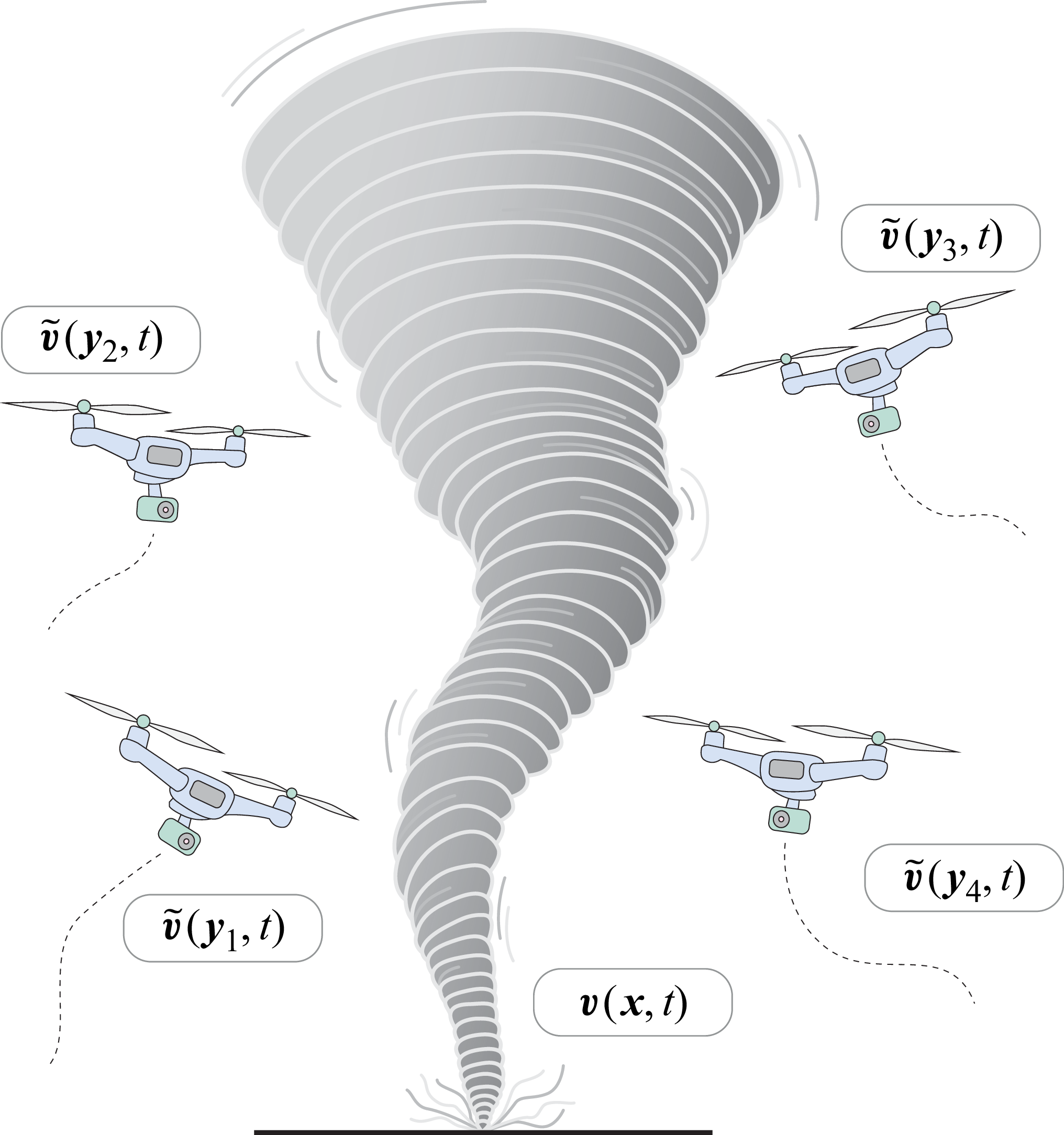


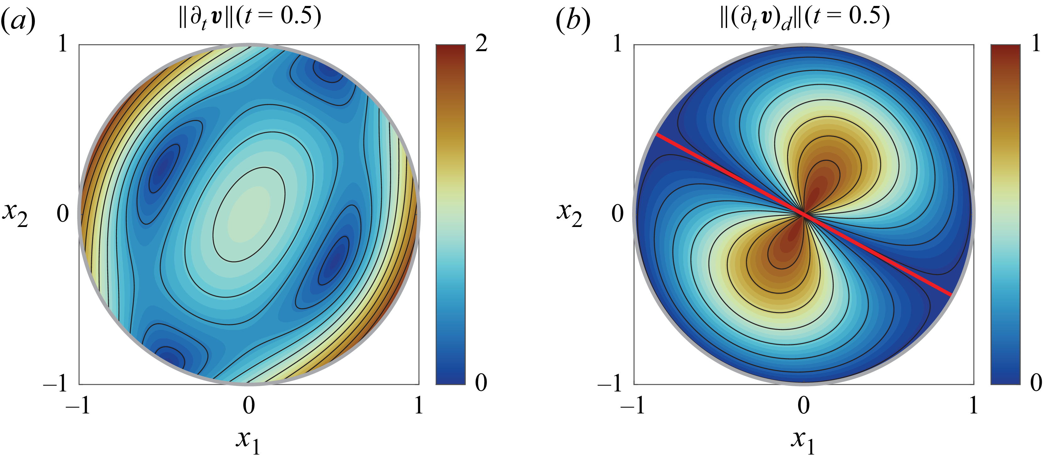
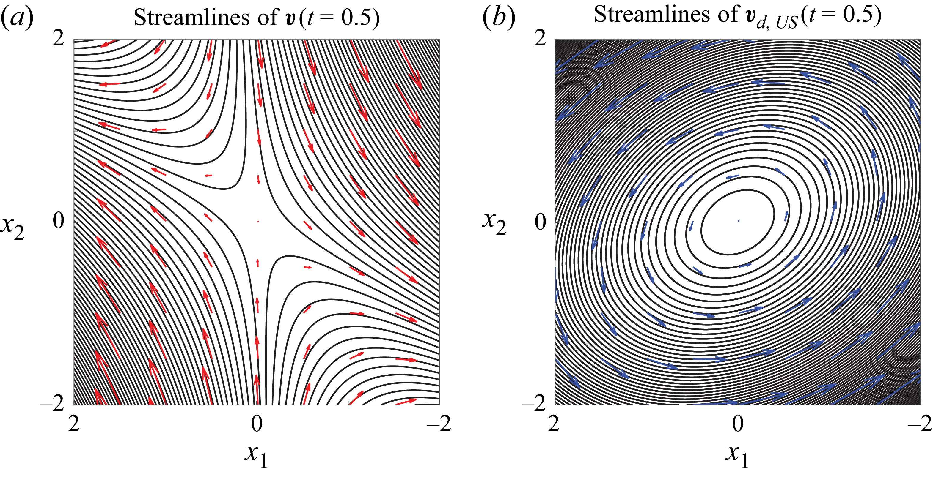


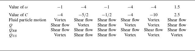

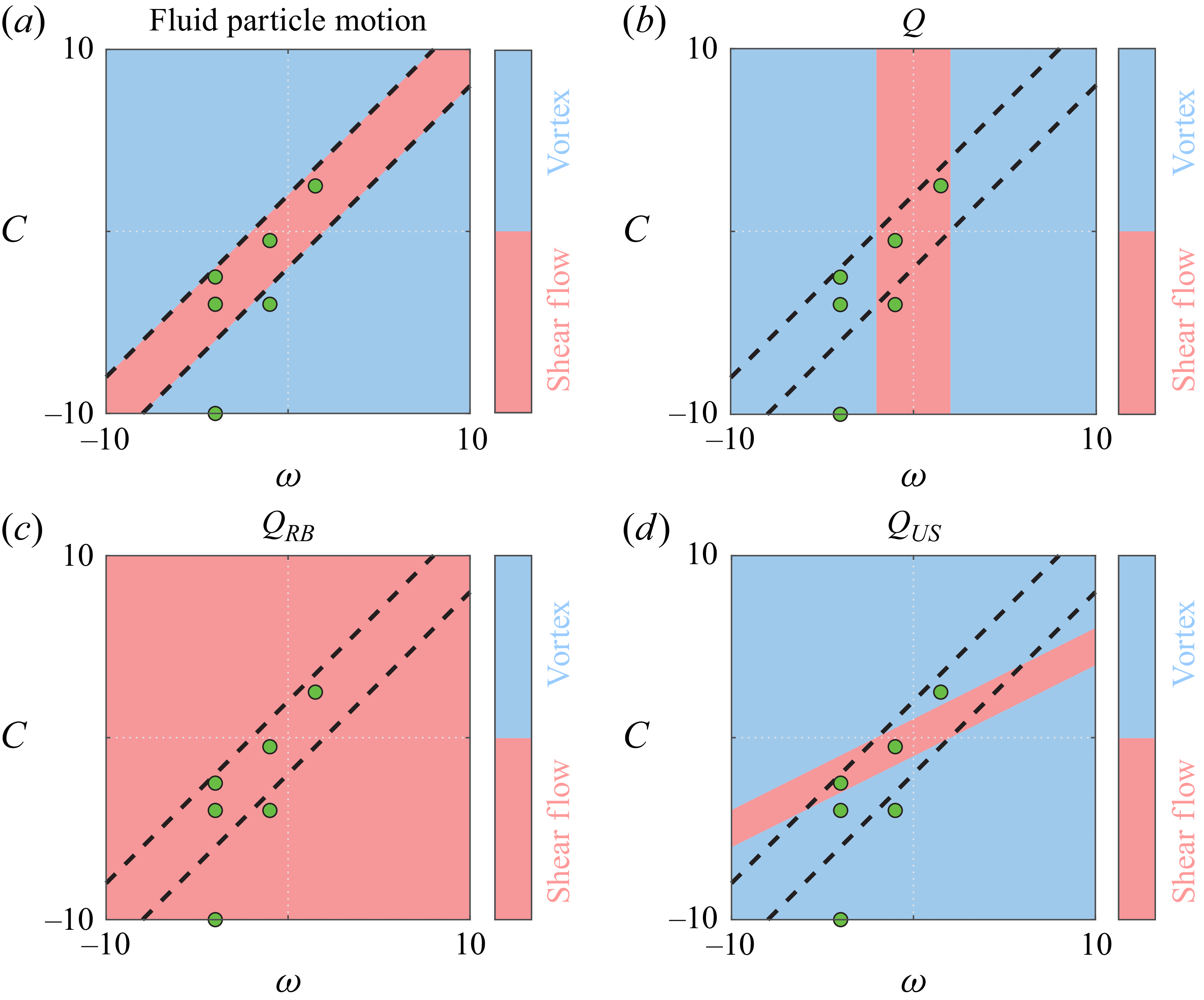


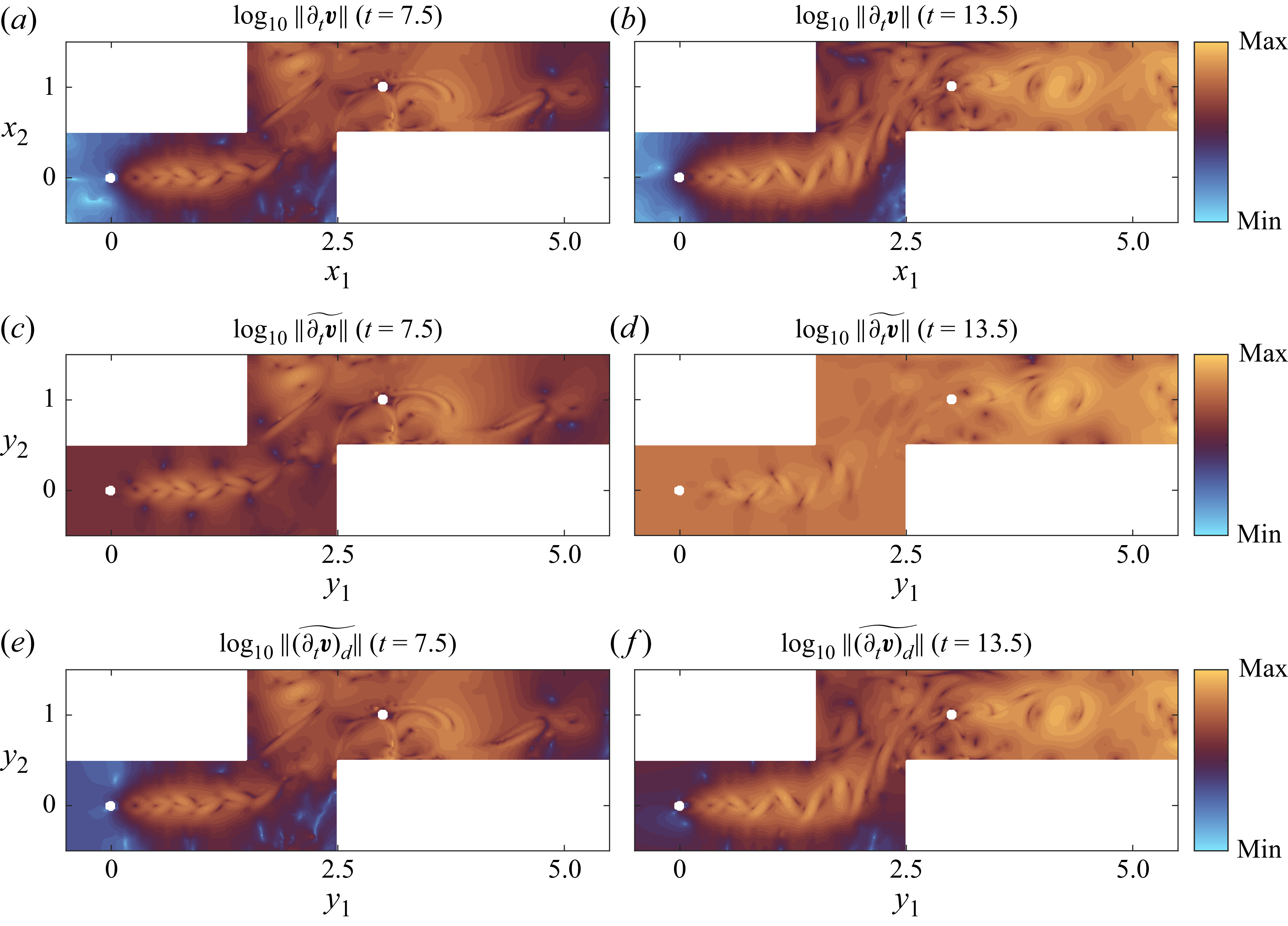


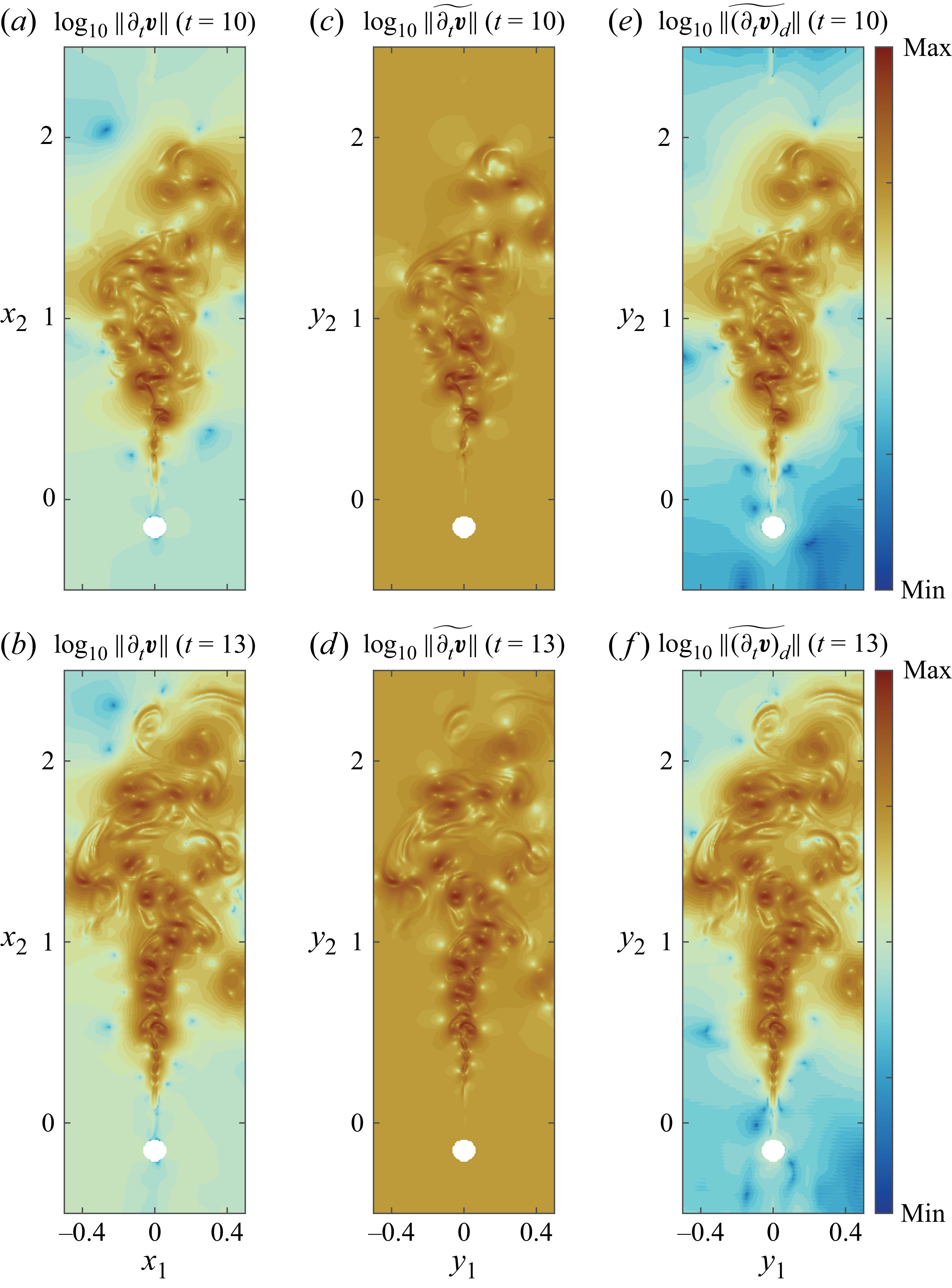


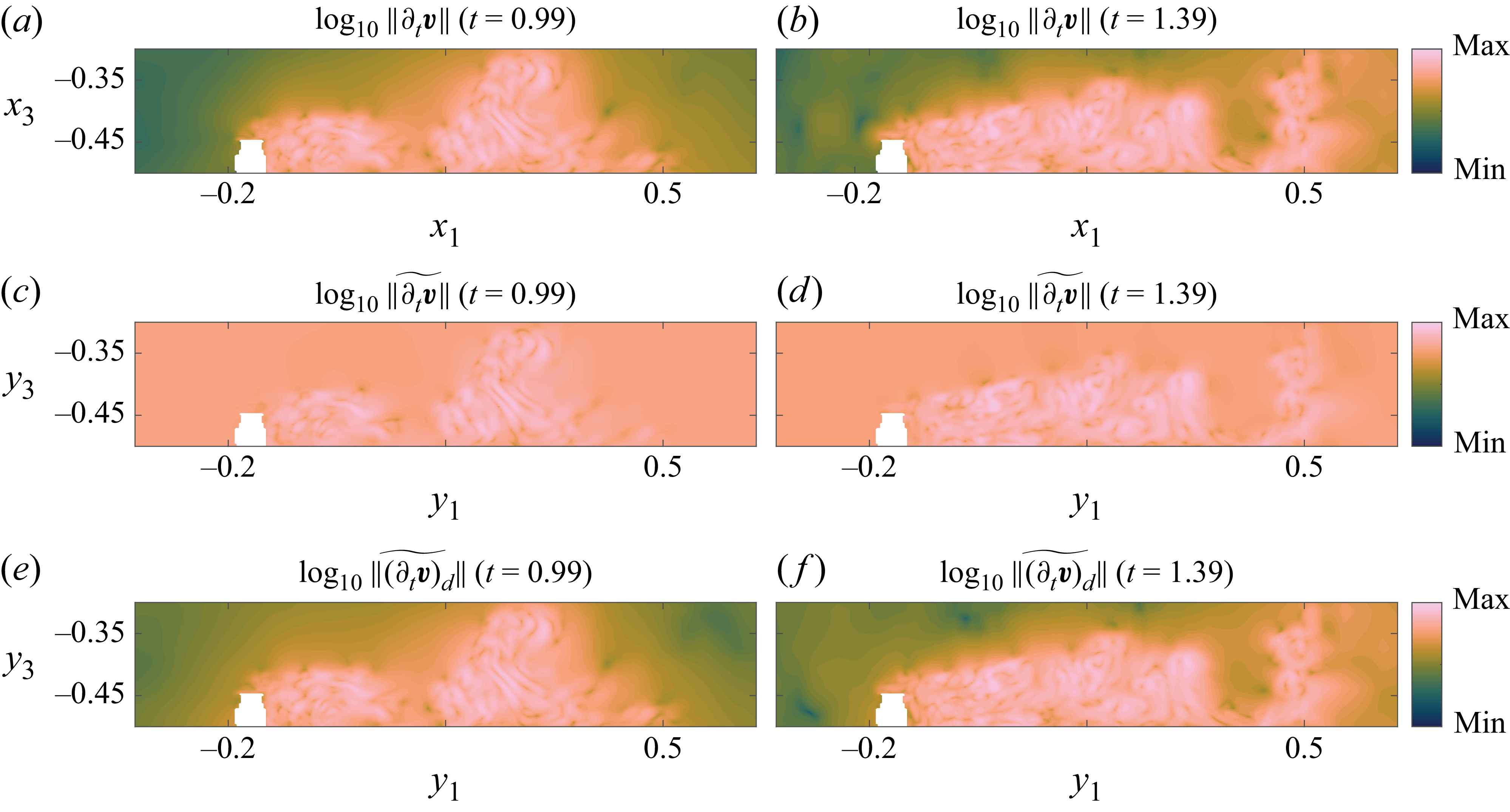


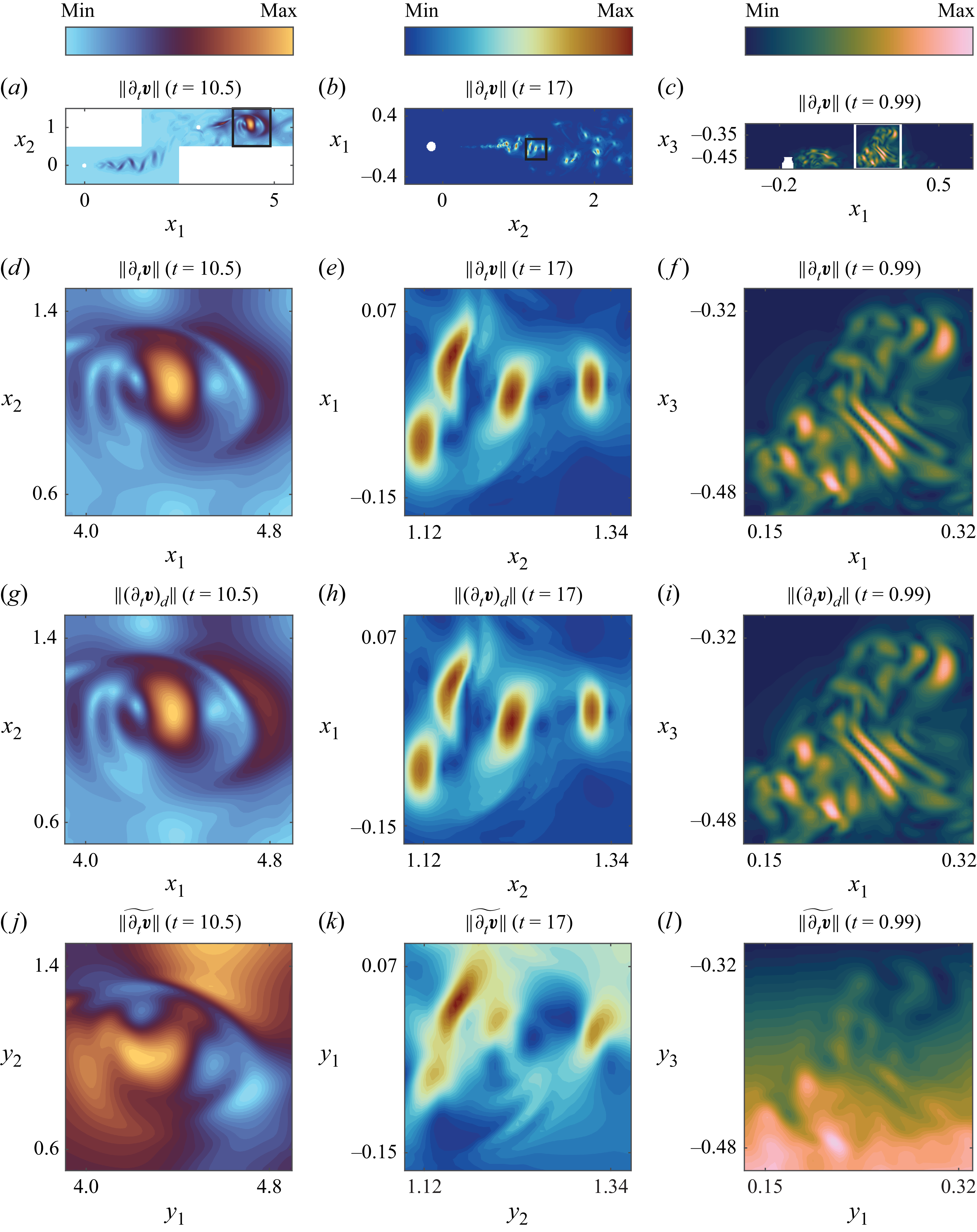


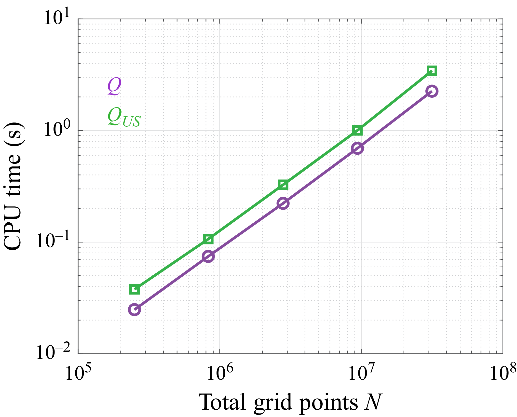


 Open access