





1. Introduction
The rapid development of industrialization and urbanization has exacerbated environmental pollution, and toxic environment poses a serious threat to the ecosystem. Toxic substances directly affect the growth, reproduction and mortality of species and change their dynamic behaviour. Developing population models can effectively predict the population trends in toxic environments and assess survival risks, such as the extinction risk of a population under pollution stress or its potential to recover to a stable state through adaptation mechanisms. This has important theoretical and practical significance for the protection of endangered species and the management of ecosystems.
Huda and Amijaya [Reference Huda, Amijaya and Purnamasari12] investigated the impact of toxins on a predator–prey system with a Holling-type functional response. Takhirov and Boborakhimova [Reference Takhirov and Boborakhimova9] established a population interaction model in a mobile, toxin-containing environment and discussed the overall solvability and free boundary behaviour of the model. Zhu and Zhang et al. [Reference Zhu, Zhang, Wang and Wang8] analyzed the bifurcation behaviour of a time-delay diffusion predator–prey model under the influence of toxins and found that toxins have a significant impact on the system dynamics. Deng, Huang, and Wang [Reference Deng, Huang and Wang23] studied the influence of toxins on the competitive dynamics of two populations in polluted water bodies, analyzed the existence and stability of spatially homogeneous steady states and found that different toxin tendencies can significantly change the system dynamics.
In biostatistics, the linear diffusion theory provides a fundamental framework for studying population migration, material transport and disease transmission. The diffusion model based on the Laplace operator can quantitatively describe the random movement of biological individuals or substances in space and predict their spatiotemporal distribution patterns. Such models not only help to understand the spatial dynamics of ecosystems but also provide guidance for practical applications such as disease control and biological conservation. Due to the ease of obtaining analytical solutions and the simplicity of their form, the linear diffusion theory has become the basis for studying nonlinear diffusion problems and has significant value in both theoretical analysis and practical modelling.
Guenad et al. [Reference Guenad, Darazirar, Djilali and Alraddadi2] investigated the existence of travelling wave solutions in a time-delay susceptible-infected-recovered (SIR) infectious disease model with generalized infection functions and proved that the basic reproduction number is the key indicator determining whether a travelling wave occurs. Bentout et al. [Reference Bentout and Djilali15] analyzed the dynamics of a susceptible-infected-susceptible (SIS) infectious disease model with general nonlinear contact rates and spatial heterogeneity, successfully establishing the asymptotic form of the endemic equilibrium under the generalized nonlinear contact rate. Nabti et al. [Reference Nabti, Djilali and Bentout1] studied a spatiotemporal virus transmission model with dual age-dependent susceptibility and infectivity, clarifying the epidemiological significance of the basic reproduction number as a threshold parameter. Djilali and Sarmad [Reference Djilali, Sarmad and Tridane17] proposed a new method for simulating SIR infectious diseases in heterogeneous environments, and the results showed that restricting the activities of infected individuals would lead to the infection concentrating in specific areas, forming ‘infection hotspots’. Djilali et al. [Reference Djilali, Darazirar and Alraddadi18] investigated the existence of travelling wave phenomena in a time-delay two-population SIR model with generalized infection functions and proved that its existence depends on the size of the basic reproduction number.
Compared with linear diffusion, the nonlinear diffusion model can more accurately describe the diffusion process of biological populations in complex environments. This model explicitly introduces the dependence of the diffusion rate on the population density, thereby reflecting the density dependence of individual movement, and can more effectively depict the adaptive response of the population to environmental heterogeneity. By dynamically adjusting the diffusion coefficient according to the population density and environmental conditions, this model can more accurately reflect the spatial distribution and migration behaviour of the population in complex environments.
Piqueras and Company [Reference Piqueras, Company and Jódar11] studied the diffusion logistic model with moving boundaries and proposed a finite difference method that preserves the properties of the theoretical solution. Sun, Chakraborty et al. [Reference Sun, Chakraborty, Liu, Jin, Anderson and Li5] conducted numerical analysis on similar models and constructed difference schemes that maintain the properties of the solutions. Colombo and Anteneodo [Reference Colombo and Anteneodo4] studied a single-species model with nonlinear diffusion and revealed the influence of nonlinearity on the phase diagram. They found that the type of diffusion determines the critical values of parameters for Turing patterns to emerge and strongly affects the shape of the patterns. Sun and Wang [Reference Sun and Wang24] used the probabilistic method to conduct asymptotic analysis on a class of stochastic logistic population models with nonlinear diffusion terms and obtained the asymptotic behaviour patterns of this class of models. Djilali, Chen et al. [Reference Djilali, Chen and Zou20] studied a heterogeneous spatiotemporal SIS infectious disease model that includes both local and nonlocal diffusion strategies and conducted steady-state analysis using the basic reproduction number as a threshold. Djilali [Reference Djilali16] studied a class of SIS infectious disease models with nonlocal diffusion and used different kernel functions in the convolution operator to distinguish the diffusion strategies of susceptibles and infectives. Djilali, Bentout et al. [Reference Djilali, Bentout and Tridane19] explored generalized nonlocal diffusion SIS models satisfying Neumann boundary conditions and spatial heterogeneity, focusing on analyzing the model properties under generalized contact rates and discussing the global asymptotic behaviour of the solutions under different diffusion coefficients.
The research on cognitive models holds significant scientific value for understanding how species adapt and cope with complex environmental challenges. Cognitive functions directly influence the behavioural patterns, foraging strategies and social interactions of species, thereby affecting their survival and reproduction in the ecosystem. Therefore, constructing cognitive models helps to explore the information processing and decision-making mechanisms of individuals under environmental stress, as well as the ways in which these cognitive processes affect population dynamics. Moreover, cognitive models can reveal the impact of environmental factors (such as toxins or resource scarcity) on the cognitive abilities of populations. This research complements the degenerate population model and together provides a more comprehensive perspective for understanding the adaptation strategies of species in response to environmental stress, thereby offering theoretical basis and practical guidance for ecosystem protection and management.
Song, Wang et al. [Reference Song, Wang and Wang27] studied a diffusion-type consumer-resource model with non-local perception, exploring the influence of non-local perception on stability and spatiotemporal patterns and observing edge oscillations and spatiotemporal chaotic phenomena under different spatial distributions. Liu, Wang et al. [Reference Liu, Wang and Zhang6] analyzed an infectious disease reaction-diffusion model with cognitive movement and nonlinear contact rate, revealing the phenomenon of separation of susceptibles and infected individuals in space. Wang and Salmaniw (2023) proposed two cognitive functions, and this paper studies one of them, namely the linear cognitive function. It was pointed out in [Reference Wang and Salmaniw7] that the cognitive function $\eta$
satisfies the following relationship:
$\eta$
satisfies the following relationship:
 \begin{equation} \bar {\eta }(x,t)=\int _{\Omega } g_R(x-y) \eta (y,t) dy, \end{equation}
Here, $g_R(x-y)$
represents the perception kernel, which depends on the perception range
$g_R(x-y)$
represents the perception kernel, which depends on the perception range $R$
. Additionally,
$R$
. Additionally, $g_R(x)$
is symmetric about the origin and monotonically decreasing from the origin, satisfying
$g_R(x)$
is symmetric about the origin and monotonically decreasing from the origin, satisfying $\int _{\Omega } g_R(x) dx = 1$
and
$\int _{\Omega } g_R(x) dx = 1$
and $\lim _{R \rightarrow 0^{+}} g_R(x) = \delta (x)$
. This paper considers the limiting case where
$\lim _{R \rightarrow 0^{+}} g_R(x) = \delta (x)$
. This paper considers the limiting case where $R \rightarrow 0^{+}$
, meaning that the perception of the population is local.
$R \rightarrow 0^{+}$
, meaning that the perception of the population is local.
This paper studies a single-species model with cognitive functions, assuming that population migration is based on cognitive memory of toxin concentration. Given that the linear diffusion model has significant limitations when describing population diffusion in complex environments – its constant diffusion rate cannot reflect the influence of density changes on diffusion behaviour – we adopt a nonlinear diffusion mechanism. Specifically, when $u \rightarrow 0$
, the degeneration condition
$u \rightarrow 0$
, the degeneration condition $G(u) \rightarrow 0$
can be interpreted as the population ceasing to move at extremely low density, which in a toxic environment may correspond to individuals losing their mobility or the group orientation when approaching the extinction threshold. This form is also consistent with the porous medium-type diffusion commonly used to describe density-dependent diffusion. This assumption can more effectively capture the population dynamics in complex environments and better reveal the population’s adaptability to environmental changes, thereby providing stronger theoretical support for studying the population survival strategies in complex ecosystems. This paper conducts an in-depth analysis of the existence of the model’s solution.
$G(u) \rightarrow 0$
can be interpreted as the population ceasing to move at extremely low density, which in a toxic environment may correspond to individuals losing their mobility or the group orientation when approaching the extinction threshold. This form is also consistent with the porous medium-type diffusion commonly used to describe density-dependent diffusion. This assumption can more effectively capture the population dynamics in complex environments and better reveal the population’s adaptability to environmental changes, thereby providing stronger theoretical support for studying the population survival strategies in complex ecosystems. This paper conducts an in-depth analysis of the existence of the model’s solution.
In the subsequent theoretical analysis, to simplify the mathematical processing and focus on the core mechanism of degenerate diffusion and toxin-cognition coupling, we model the cognitive process as a point-state memory model, which is described by the local ordinary differential equation $\eta _t = bw - \gamma \eta$
. This can be regarded as the limiting case of the non-local perception kernel
$\eta _t = bw - \gamma \eta$
. This can be regarded as the limiting case of the non-local perception kernel $g_R$
when the perception range
$g_R$
when the perception range $R \rightarrow 0$
, and the core still retains the biological idea of ‘adjusting behaviour based on toxin’.
$R \rightarrow 0$
, and the core still retains the biological idea of ‘adjusting behaviour based on toxin’.
It is worth noting that, compared with classical chemotaxis models or the chemotaxis–haptotaxis model in [Reference Fagioli, Radici and Romagnoli21], the coupling structure of our system exhibits essential differences. The toxin concentration $w$
not only decays linearly via
$w$
not only decays linearly via $-gw$
but also couples strongly with the population density
$-gw$
but also couples strongly with the population density $u$
through the absorption term
$u$
through the absorption term $-luw$
, while simultaneously serving as the driving source for the cognitive function
$-luw$
, while simultaneously serving as the driving source for the cognitive function $\eta$
(
$\eta$
( $\eta _t = b w - \gamma \eta$
). This
$\eta _t = b w - \gamma \eta$
). This $u$
-
$u$
- $w$
-
$w$
- $\eta$
triangular coupling introduces new mathematical challenges: in the a priori estimates, the cross-term
$\eta$
triangular coupling introduces new mathematical challenges: in the a priori estimates, the cross-term $luw$
and its gradient appear in multiple energy inequalities, making standard interpolation techniques difficult to apply directly. Hence, the main difficulty lies not merely in the degenerate diffusion itself but also in controlling the coupling generated by the toxin absorption term and the cognition-related cross-effects. To overcome this difficulty, in Section 3, we carefully coordinate the interpolation exponents of each variable, fully utilize the established
$luw$
and its gradient appear in multiple energy inequalities, making standard interpolation techniques difficult to apply directly. Hence, the main difficulty lies not merely in the degenerate diffusion itself but also in controlling the coupling generated by the toxin absorption term and the cognition-related cross-effects. To overcome this difficulty, in Section 3, we carefully coordinate the interpolation exponents of each variable, fully utilize the established $L^1$
and
$L^1$
and $L^p$
estimates and progressively separate and control these coupling terms to establish uniform boundedness. One- and two-dimensional numerical experiments further illustrate the cognition-driven toxin avoidance behaviour, providing a concrete visualization of the system dynamics.
$L^p$
estimates and progressively separate and control these coupling terms to establish uniform boundedness. One- and two-dimensional numerical experiments further illustrate the cognition-driven toxin avoidance behaviour, providing a concrete visualization of the system dynamics.
The structure of this paper is as follows: Section 2 introduces the model and studies the local existence of its weak solution through regularization; Section 3 provides the a priori estimates for the system; Section 4 analyzes the boundary problems of the regularized system; Section 5 obtains the global existence of the weak solution of the original system and the last section conducts numerical simulations of the theoretical results.
2. Local existence of the weak solution of the regularized model
This section is dedicated to studying the mathematical modelling of degraded systems and the existence of solutions. Specifically, we first present the mathematical model and then establish the local-in-time existence of weak solutions. We consider the following model:
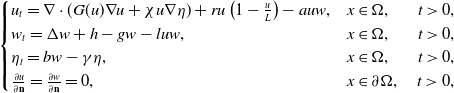 \begin{equation} \begin{cases} u_t=\nabla \cdot (G(u) \nabla u+\chi u \nabla \eta )+r u\left (1-\frac {u}{L}\right )-a u w, &x \in \Omega ,\quad\,\,\, t\gt 0, \\ w_t=\Delta w+h-g w-l u w, &x \in \Omega ,\quad\,\,\, t\gt 0,\\ \eta _t=b w-\gamma \eta ,&x \in \Omega ,\quad\,\,\, t\gt 0,\\ \frac {\partial u}{\partial \mathbf{n}}=\frac {\partial w}{\partial \mathbf{n}}=0, &x \in \partial \Omega ,\quad t\gt 0, \end{cases} \end{equation}
where $G(u)$
is a nonlinear function satisfying the following assumptions:
$G(u)$
is a nonlinear function satisfying the following assumptions: $\mathbf{(H1)}$ $G \in C^2([0, \infty )), G(s) \geqslant 0$
, for all
$G \in C^2([0, \infty )), G(s) \geqslant 0$
, for all $s \geqslant 0$
.
$s \geqslant 0$
. $\mathbf{(H2)}$
There exist some constants
$\mathbf{(H2)}$
There exist some constants $\gamma \gt 1$
and
$\gamma \gt 1$
and $k_G\gt 0$
such that
$k_G\gt 0$
such that $G(s) \geqslant k_G s^{\gamma -1}$
for all
$G(s) \geqslant k_G s^{\gamma -1}$
for all $s \geqslant 0$
.
$s \geqslant 0$
.
And we denote by $\Psi$
the primitive function of
$\Psi$
the primitive function of $G$
, namely
$G$
, namely $\Psi (u)=\int _0^u G(s) \mathrm{d} s$
. Assume that the initial data
$\Psi (u)=\int _0^u G(s) \mathrm{d} s$
. Assume that the initial data $u(x, 0)=u_0(x), w(x, 0)=w_0(x), \eta (x, 0)=\eta _0(x)$
system (2.1) satisfy a standard compatibility condition in the sense that
$u(x, 0)=u_0(x), w(x, 0)=w_0(x), \eta (x, 0)=\eta _0(x)$
system (2.1) satisfy a standard compatibility condition in the sense that
 \begin{equation} \begin{cases} u_0 \in W^{1, \infty }(\Omega ) \text{ with } u_0 \geqslant 0 \text{ in } \Omega \text{ and } u_0 \neq 0, \\ w_0 \in W^{1, \infty }(\Omega ) \text{ with } 0 \leqslant w_0 \leqslant h \text{ in } \Omega \text{ and } \frac {\partial w_0}{\partial \nu }=0 \text{ on } \partial \Omega , \\ \eta _0 \in C^{2+\vartheta }(\bar {\Omega }) \text{ with } 0 \leqslant \eta _0 \leqslant b h \text{ in } \bar {\Omega } \end{cases} \end{equation}
for some $\vartheta \in (0,1)$
and
$\vartheta \in (0,1)$
and $h\gt 0$
. The population density
$h\gt 0$
. The population density $u(x,t)$
follows a logistic growth law with nonlinear diffusion, and its evolution process is doubly regulated by the toxin concentration
$u(x,t)$
follows a logistic growth law with nonlinear diffusion, and its evolution process is doubly regulated by the toxin concentration $w(x,t)$
and cognitive ability
$w(x,t)$
and cognitive ability $\eta (x,t)$
. In terms of cognitive mechanisms, the population remembers the spatial distribution information of toxins at a rate of
$\eta (x,t)$
. In terms of cognitive mechanisms, the population remembers the spatial distribution information of toxins at a rate of $b$
and forgets historical information at a rate of
$b$
and forgets historical information at a rate of $\gamma$
. This process is achieved through the cognitive function
$\gamma$
. This process is achieved through the cognitive function $\eta (x,t)$
. Toxicokinetics involves three key processes: continuous input into the environment at a rate of
$\eta (x,t)$
. Toxicokinetics involves three key processes: continuous input into the environment at a rate of $h$
, degradation by the environment at a rate of
$h$
, degradation by the environment at a rate of $g$
and absorption by the population at a rate of
$g$
and absorption by the population at a rate of $l$
. In particular, parameter
$l$
. In particular, parameter $a$
quantitatively characterizes the intensity of damage caused by toxins to the population.
$a$
quantitatively characterizes the intensity of damage caused by toxins to the population.
Before we give the main results, we first introduce the definition of solution of system (2.1).
Definition 2.1. If
 \begin{equation*} \begin{gathered} (u, w, \eta ) \in L_{l o c}^2(0, T ;\, L^2(\Omega )) \times L_{l o c}^2 (0, T ;\, W^{1,2}(\Omega )) \times L_{l o c}^2(0, T ;\, W^{1,2}(\Omega ) ) \\ G(u) \nabla mu \in L_{l o c}^1(0, T ;\, L^1(\Omega ) ) \end{gathered} \end{equation*}
and for any $\Phi \in C_0^{\infty }(\bar {\Omega } \times [0, T))$
, it holds that
$\Phi \in C_0^{\infty }(\bar {\Omega } \times [0, T))$
, it holds that
 \begin{equation*} \begin{aligned} -\int _0^T \int _{\Omega } u \Phi _t \mathrm{\,d} x \mathrm{\,d} t-\int _{\Omega } u_0 \phi (x, 0) \mathrm{d} x= & -\int _0^T \int _{\Omega } G(u) \nabla u \nabla \Phi \mathrm{\,d} x \mathrm{\,d} t \\ & +\chi \int _0^T \int _{\Omega } f(u) \nabla \eta \nabla \Phi \mathrm{\,d} x \mathrm{\,d} t+\int _0^T \int _{\Omega } U(u) \Phi \mathrm{d} x \mathrm{\,d} t, \end{aligned} \end{equation*}
 \begin{equation*}\quad -\int _0^T \int _{\Omega } w \Phi _t \mathrm{\,d} x \mathrm{\,d} t-\int _{\Omega } w_0 \phi (x, 0) \mathrm{d} x=-\int _0^T \int _{\Omega } \nabla w \nabla \Phi \mathrm{\,d} x \mathrm{\,d} t+\int _0^T \int _{\Omega }(h-g w-l u w) \Phi \mathrm{d} x \mathrm{\,d} t, \end{equation*}
 \begin{align*} \qquad\qquad\!\quad -\int _0^T \int _{\Omega } \eta \Phi _t \mathrm{\,d} x \mathrm{\,d} t-\int _{\Omega } \eta _0 \Phi (x, 0) \mathrm{d} x=\int _0^T \int _{\Omega } \left (b w-\gamma \eta \right )\Phi \mathrm{d} x \mathrm{\,d} t, \end{align*}
then $(u, w, \eta )$
is a local solution of (
2.1
) on
$(u, w, \eta )$
is a local solution of (
2.1
) on $({\Omega } \times [0, T))$
. If
$({\Omega } \times [0, T))$
. If $T=\infty$
, then
$T=\infty$
, then $(u, w, \eta )$
is a global solution of (
2.1
).
$(u, w, \eta )$
is a global solution of (
2.1
).
Existence and boundedness of global weak solutions to system (2.1) will be proved by introducing a proper regularized (non-degenerate) problem for which we are able to construct a global classical solution. Moreover, the regularized system admits enough regularity that allows one to pass to the limit in the regularization parameter. In order to do so, for $\iota \in (0,1)$
, we introduce the function
$\iota \in (0,1)$
, we introduce the function $G_\iota$
defined by
$G_\iota$
defined by
 \begin{equation} G_\iota (s)=G(s+\iota ). \end{equation}
Note that, according to Assumptions $\mathbf{(H1)}-\mathbf{(H2)}$
, we have that
$\mathbf{(H1)}-\mathbf{(H2)}$
, we have that $G_\iota (s) \geqslant k_G(s+\iota )^{\gamma -1}$
and
$G_\iota (s) \geqslant k_G(s+\iota )^{\gamma -1}$
and $G_\iota (0)\gt 0$
. Moreover, the primitive of
$G_\iota (0)\gt 0$
. Moreover, the primitive of $G_\iota$
is given by
$G_\iota$
is given by
 \begin{equation} \Psi _\iota (s)=\int _{-\iota }^{s-\iota } G_\iota (\zeta ) \mathrm{d} \zeta =\int _0^s G(\zeta ) \mathrm{d} \zeta \!. \end{equation}
Given a triple $\left (u_0, w_0, \eta _0\right )$
satisfying (2.2), we define
$\left (u_0, w_0, \eta _0\right )$
satisfying (2.2), we define $\left (u_{\iota 0}, w_{\iota 0}, \eta _{\iota 0}\right )$
such that, for some
$\left (u_{\iota 0}, w_{\iota 0}, \eta _{\iota 0}\right )$
such that, for some $\vartheta \in (0,1)$
,
$\vartheta \in (0,1)$
,
 \begin{equation} u_{\iota 0}, w_{\iota 0}, \eta _{\iota 0} \in C^{2+\vartheta }(\bar {\Omega }), 0 \leqslant \eta _{\iota 0} \leqslant 1,\quad \text{ and }\quad\left .\frac {\partial u_{\iota 0}}{\partial \mathbf{n}}\right |_{\partial \Omega }=\left .\frac {\partial w_{\iota 0}}{\partial \mathbf{n}}\right |_{\partial \Omega }=0 \end{equation}
and
 \begin{equation*} u_{\iota 0} \rightarrow m_0, w_{\iota 0} \rightarrow w_0, \eta _{\iota 0} \rightarrow \eta _0, \text{ uniformly. } \end{equation*}
For $T\gt 0$
, we consider the following regularized system
$T\gt 0$
, we consider the following regularized system
 \begin{equation} \begin{cases} u_{\iota t}=\nabla \cdot (G(u_{\iota }) \nabla u_{\iota }+\chi f(u_{\iota }) \nabla \eta )+U(u_{\iota }), &x \in \Omega , t\gt 0, \\ w_{\iota t}=\Delta w_{\iota }+h-g w_{\iota }-l u_{\iota } w_{\iota }, &x \in \Omega , t\gt 0,\\ \eta _{\iota t}=b w_{\iota }-\gamma \eta _{\iota },&x \in \Omega , t\gt 0, \end{cases} \end{equation}
with $(x, t) \in \Omega _T$
, under the initial conditions
$(x, t) \in \Omega _T$
, under the initial conditions
 \begin{equation*} u_\iota (x, 0)=u_{\iota 0}(x), w_\iota (x, 0)=w_{\iota 0}(x), \eta _\iota (x, 0)=\eta _{\iota 0}(x). \end{equation*}
System (2.6) is endowed with the Neumann boundary conditions
 \begin{equation*} \left .\frac {\partial u_\iota }{\partial \mathbf{n}}\right |_{\partial \Omega }=\left .\frac {\partial w_\iota }{\partial \mathbf{n}}\right |_{\partial \Omega }=0. \end{equation*}
Then, by applying the fixed-point theorem and the existence theorem for linear parabolic equations, we can obtain the global existence of the weak solution for the model (2.1).
Theorem 2.1.
Let $\iota \in (0,1)$
and
$\iota \in (0,1)$
and $\chi \gt 0$
. Assume that the nonnegative functions
$\chi \gt 0$
. Assume that the nonnegative functions $u_{\iota 0}, w_{\iota 0}$
and
$u_{\iota 0}, w_{\iota 0}$
and $\eta _{\iota 0}$
satisfy (
2.6
) for some
$\eta _{\iota 0}$
satisfy (
2.6
) for some $\iota \in (0,1)$
. Consider
$\iota \in (0,1)$
. Consider $G_{\iota }$
as in (
2.3
). Then, there exists a maximal existence time
$G_{\iota }$
as in (
2.3
). Then, there exists a maximal existence time $T_{\text{max}} \in (0, \infty ]$
and a triple of nonnegative functions
$T_{\text{max}} \in (0, \infty ]$
and a triple of nonnegative functions
 \begin{equation*} \begin{gathered} u_{\iota } \in C^0(\bar {\Omega } \times [0, T_{\max }) ) \cap C^{2,1}(\bar {\Omega } \times (0, T_{\max }) ), \\ w_{\iota } \in C^0(\bar {\Omega } \times [0, T_{\max }) ) \cap C^{2,1}(\bar {\Omega } \times (0, T_{\max })), \\ \eta _{\iota } \in C^{2,1}(\bar {\Omega } \times (0, T_{\max })) \end{gathered} \end{equation*}
that solves (
2.6
) classically on $\Omega \times \left (0, T_{\max }\right )$
and satisfies
$\Omega \times \left (0, T_{\max }\right )$
and satisfies $0 \leqslant \eta _{\iota } \leqslant \left \|\eta _{{\iota }0}\right \|_{L^{\infty }(\Omega )}, u_{\iota } \geqslant 0$
and
$0 \leqslant \eta _{\iota } \leqslant \left \|\eta _{{\iota }0}\right \|_{L^{\infty }(\Omega )}, u_{\iota } \geqslant 0$
and $w_{\iota } \geqslant 0$
in
$w_{\iota } \geqslant 0$
in $\Omega \times \left (0, T_{\max }\right )$
. Moreover, either
$\Omega \times \left (0, T_{\max }\right )$
. Moreover, either $T_{\max }=+\infty$
or
$T_{\max }=+\infty$
or
 \begin{equation} \left \|u_{\iota }(\cdot , t)\right \|_{L^{\infty }(\Omega )}+\left \|w_{\iota }(\cdot , t)\right \|_{W^{1,\infty } (\Omega )}+\left \|\eta _{\iota }(\cdot , t)\right \|_{L^{\infty }(\Omega )} \rightarrow \infty \text{ as } t \nearrow T_{\max }. \end{equation}
According to the above existence theory, for any $s \in \left (0, T_{\!\max }\right ),\left (u_{\iota }(\cdot , s), w_{\iota }(\cdot , s), \eta _{\iota }(\cdot , s)\right ) \in C^2(\bar {\Omega })$
. Without loss of generality, we can assume that there exists a positive constant
$s \in \left (0, T_{\!\max }\right ),\left (u_{\iota }(\cdot , s), w_{\iota }(\cdot , s), \eta _{\iota }(\cdot , s)\right ) \in C^2(\bar {\Omega })$
. Without loss of generality, we can assume that there exists a positive constant $K$
such that
$K$
such that
 \begin{equation} \left \|u_{{\iota } 0}\right \|_{C^2(\Omega )}+\left \|w_{{\iota } 0}\right \|_{C^2(\Omega )}+\left \|\eta _{{\iota } 0}\right \|_{C^2(\Omega )} \leqslant K . \end{equation}
3. Prior estimate of the regularized system
In this section, we derive a priori estimates for the regularized system. These estimates provide essential insights into the behaviour of the solutions and lay the groundwork for further analysis, including the convergence and stability of the regularized system.
Lemma 3.1.
There exists a positive constant $K_0$
only depending on
$K_0$
only depending on $\Omega$
and
$\Omega$
and $\left \|u_{{\iota } 0}\right \|_{L^1(\Omega )}$
such that the solution
$\left \|u_{{\iota } 0}\right \|_{L^1(\Omega )}$
such that the solution $\left (u_{\iota }, w_{\iota }, \eta _{\iota }\right )$
of (
2.6
) satisfies
$\left (u_{\iota }, w_{\iota }, \eta _{\iota }\right )$
of (
2.6
) satisfies
 \begin{equation} \left \|u_{\iota }(\cdot , t)\right \|_{L^1(\Omega )} \leqslant K_0 \text{ for all } t \in \left (0, T_{\max }\right )\! . \end{equation}
Moreover, if $U=0$
$U=0$
 \begin{equation} \left \|u_{\iota }(\cdot , t)\right \|_{L^1(\Omega )}=\left \|u_{{\iota } 0}\right \|_{L^1(\Omega )} \text{ for all } t \in \left (0, T_{\max }\right ) \!. \end{equation}
Proof. Using Hölder inequality, we can get
 \begin{equation*} \begin{aligned} \int _{\Omega } u_\iota &\leqslant \left (\int _{\Omega }1^2\right )^{\frac {1}{2}} \left (\int _{\Omega } u_\iota ^2\right )^{\frac {1}{2}}\\ &\leqslant |\Omega |^{\frac {1}{2}} \left (\int _{\Omega } u_\iota ^{\frac {1}{2}}\right )\!, \end{aligned} \end{equation*}
which implies that
 \begin{equation} \int _{\Omega } u_\iota ^2 \geqslant \frac {1}{|\Omega |^{\frac {1}{2}}}\left (\int _{\Omega } u_\iota \right )^2\!. \end{equation}
From the first equation of (2.6), Green formula and (3.3) yield
 \begin{equation*} \begin{aligned} \int _{\Omega } \frac {d}{d t} u_{\iota }&=\int _{\Omega } \nabla \left (G_\iota \left (u_\iota \right ) \nabla u_\iota \right )u_\iota + \chi \int _{\Omega } \nabla \left (f\left (u_\iota \right )\nabla \eta _\iota \right ) + \int _{\Omega } U\left (u_\iota \right ) \\ &=\int _{\Omega } U\left (u_\iota \right )=\int _{\Omega } \left (r u\left (1-\frac {u}{L}\right )-a u w\right )\\ &\leqslant \int _{\Omega } r u_\iota - \frac {r}{|\Omega | K} \left (\int _{\Omega } u_\iota \right )^2\!, \end{aligned} \end{equation*}
Then, according to the comparison principle, we have
 \begin{equation*}\|u_\iota (\cdot , t)\|_{L_1(\Omega )} \leqslant \max {\int _{\Omega } u_{\iota 0},\ \ |\Omega |}\,:\!=\,K_0.\end{equation*}
Obviously, if $U=0$
, we have the conservation of
$U=0$
, we have the conservation of $L^1$
-norm. The proof is complete.
$L^1$
-norm. The proof is complete.
Next prove that the third equation of (2.6) is also bounded.
Lemma 3.2.
For any $p \geqslant 1$
, the solution
$p \geqslant 1$
, the solution $\left (u_{\iota }, w_{\iota }, \eta _{\iota }\right )$
to (
2.6
) satisfies
$\left (u_{\iota }, w_{\iota }, \eta _{\iota }\right )$
to (
2.6
) satisfies
 \begin{equation} \eta _{\iota } \leqslant b h, \text{ for all } t \in \left (0, T_{\max }\right )\!, x \in \Omega \end{equation}
Proof. The constant variation method and the third equation of (2.6) show that
 \begin{equation*} \eta _\iota =e^{-\gamma t}\left [\int _0^t b w_\iota e^{\gamma t} + c\right ]\\ \leqslant e^{-\gamma t} \left [\int _0^t b h e^{\gamma t} + c\right ]\!. \end{equation*}
It is worth mentioning that when $t=0$
,
$t=0$
, $\eta _{\iota 0} \leqslant b h$
. This proof is complete.
$\eta _{\iota 0} \leqslant b h$
. This proof is complete.
By multiplying the third equation of (2.6) by $\eta _\iota ^{p-1}$
, using the Young’s inequality, we are able to produce the following estimate.
$\eta _\iota ^{p-1}$
, using the Young’s inequality, we are able to produce the following estimate.
Lemma 3.3.
For any $p \geqslant 1$
, the solution
$p \geqslant 1$
, the solution $\left (u_{\iota }, w_{\iota }, \eta _{\iota }\right )$
to (
2.6
) satisfies
$\left (u_{\iota }, w_{\iota }, \eta _{\iota }\right )$
to (
2.6
) satisfies
 \begin{equation} \frac {1}{p} \frac {\mathrm{\,d}}{\mathrm{\,d} t} \int _{\Omega } \eta _\iota { }^p \mathrm{\,d} x \leqslant \frac {p-1}{p} \int _{\Omega } \eta _\iota { }^p \mathrm{\,d} x, \end{equation}
for all $t \in \left (0, T_{\max }\right )$
. In particular,
$t \in \left (0, T_{\max }\right )$
. In particular,
 \begin{equation*} \left \|\eta _{\iota }\right \|_{L^1(\Omega )} \leqslant b h \end{equation*}
for all $t \in (0, T_{\text{max}})$
, where
$t \in (0, T_{\text{max}})$
, where $K_0$
is the constant introduced in Lemma
3.1
.
$K_0$
is the constant introduced in Lemma
3.1
.
At this point, we want to derive a uniform upper bound for $u_\iota$
, which represents the key to obtain all the higher-order estimates and thus to extend the classical solution globally.
$u_\iota$
, which represents the key to obtain all the higher-order estimates and thus to extend the classical solution globally.
Lemma 3.4.
Let $\sigma ,\chi \gt 0$
and
$\sigma ,\chi \gt 0$
and $\gamma \gt 1$
be given constants. Then, for any
$\gamma \gt 1$
be given constants. Then, for any $p\gt 1$
, the solution
$p\gt 1$
, the solution $\left (u_\iota , w_\iota , \eta _\iota \right )$
to (
2.6
) satisfies
$\left (u_\iota , w_\iota , \eta _\iota \right )$
to (
2.6
) satisfies
 \begin{align} \frac {1}{p} \frac {\,d}{d t}\int _{\Omega } u_\iota { }^p \mathrm{\,d} x &+\frac {p-1}{2} \int _{\Omega } G_{\iota }\left (u_{\iota }\right ) \left |\nabla u_{\iota }\right |^2 u_{\iota }^{p-2} \mathrm{\,d} x +\frac {k_G(p-1)}{\left (p+\gamma -1\right )^2} \int _{\Omega } |\nabla u_\iota { }^{\frac {p+\gamma -1}{2}}|^2 \mathrm{\,d} x\nonumber\\ &\leqslant \frac {\chi ^2 (p-1)}{k_G} \int _{\Omega } u_\iota ^{p-\gamma +1}\left |\nabla \eta _\iota \right |^2 \mathrm{\,d} x + \sigma \int _{\Omega } u_\iota ^p \mathrm{\,d} x - \sigma \int _{\Omega } u_\iota ^{p+1} \mathrm{\,d} x \end{align}
for all t $\in \left (0, T_{\max }\right )$
.
$\in \left (0, T_{\max }\right )$
.
Proof. Multiplying the first equation of (2.6) by $u_\iota { }^{p-1}$
and integrating yields
$u_\iota { }^{p-1}$
and integrating yields
 \begin{align} \frac {1}{p} \frac {\,d}{d t}\int _{\Omega } u_\iota { }^p \mathrm{\,d} x&= \int _{\Omega } \nabla \left (G_\iota \left (u_\iota \right )\nabla u_\iota \right ) u_\iota { }^{p-1} \mathrm{\,d} x+ \chi \int _{\Omega } \nabla \left (f(u_\iota ) \nabla \eta _\iota \right ) u_\iota { }^{p-1} +\mathrm{\,d} x \int _{\Omega } U_\iota (u_\iota ) u_\iota { }^{p-1}\mathrm{\,d} x\nonumber\\ &\leqslant -\left (p-1\right ) \int _{\Omega } G_\iota (u_\iota ) |\nabla u_\iota |^2 u_\iota { }^{p-2}\mathrm{\,d} x + \chi \left (p-1\right ) \int _{\Omega } f(u_\iota ) \nabla \eta _\iota u_\iota { }^{p-2} \cdot \nabla u_\iota \mathrm{\,d} x\nonumber\\ & \ \ \ +\int _{\Omega } U(u_\iota ) u_\iota { }^{p-1} \mathrm{\,d} x\,:\!=\, I_1 + I_2 + I_3 \end{align}
on $t \in \left (0, T_{\text{max}}\right )$
. Below we analyze each
$t \in \left (0, T_{\text{max}}\right )$
. Below we analyze each $I_1, I_2, I_3$
. We first estimate the term involving the nonlinear diffusion as follows
$I_1, I_2, I_3$
. We first estimate the term involving the nonlinear diffusion as follows
 \begin{equation} I_1 \leqslant -\frac {p-1}{2} \int _{\Omega } G_{\iota }\left (u_{\iota }\right ) \left |\nabla u_{\iota }\right |^2 u_{\iota }^{p-2} \mathrm{\,d} x-\frac {p-1}{2} k_G \int _{\Omega } u_{\iota }^{p-2}\left (u_{\iota }+c\right )^{\gamma -1}\left |\nabla u_{\iota }\right |^2 \mathrm{\,d}{x}. \end{equation}
Then, we derive the following estimate by integrating by parts on $I_2$
and applying Young’s inequality
$I_2$
and applying Young’s inequality
 \begin{equation} \begin{aligned} I_2 &\leqslant \frac {k_G(p-1)}{4} \int _{\Omega } u_\iota ^{\gamma +p-3}\left |\nabla u_\iota \right |^2 \mathrm{\,d} x+\frac {\chi ^2 (p-1)}{k_G} \int _{\Omega } u_\iota ^{p-\gamma +1}\left |\nabla \eta _\iota \right |^2 \mathrm{\,d} x. \end{aligned} \end{equation}
By combining Equations (3.8) and (3.9), we can derive the following expression:
 \begin{align} &\ \ \ \frac {1}{p} \frac {\,d}{d t}\int _{\Omega } u_\iota { }^p \mathrm{\,d} x +\frac {p-1}{2} \int _{\Omega } G_{\iota }\left (u_{\iota }\right ) \left |\nabla u_{\iota }\right |^2 u_{\iota }^{p-2} \mathrm{\,d} x\nonumber\\ &\leqslant -\frac {p-1}{2} k_G \int _{\Omega } u_{\iota }^{p-2}\left (u_{\iota }+c\right )^{\gamma -1}\left |\nabla u_{\iota }\right |^2 \mathrm{\,d}{x} +\frac {k_G(p-1)}{4} \int _{\Omega } u_\iota ^{\gamma +p-3}\left |\nabla u_\iota \right |^2 \mathrm{\,d} x\nonumber\\ &\ \ \ +\frac {\chi ^2 (p-1)}{k_G} \int _{\Omega } u_\iota ^{p-\gamma +1}\left |\nabla \eta _\iota \right |^2 \mathrm{\,d} x + \int _{\Omega } r u_\iota ^p \mathrm{\,d} x - \frac {r}{L}\int _{\Omega } u_\iota ^{p+1} \mathrm{\,d} x, \end{align}
then using
 \begin{equation*}|\nabla u_{\frac {p+\gamma -1}{2}}|^2=\frac {\left (p+\gamma -1\right )^2}{4} u^{p+\gamma -3} |\nabla u_\iota |^2\end{equation*}
we derive
 \begin{align} &-\frac {p-1}{2} k_G \int _{\Omega } u_{\iota }^{p-2}\left (u_{\iota }+c\right )^{\gamma -1}\left |\nabla u_{\iota }\right |^2 \mathrm{\,d}{x} +\frac {k_G(p-1)}{4} \int _{\Omega } u_\iota ^{\gamma +p-3}\left |\nabla u_\iota \right |^2 \mathrm{\,d} x \nonumber\\ &\lt \frac {-k_G \left (p-1\right )}{\left (p+\gamma -1\right )^2} \int _{\Omega } |\nabla u_\iota ^{\frac {p+\gamma -1}{2}}|^2 \mathrm{\,d} x. \end{align}
Combining (3.10) and (3.11), (3.6) can be readily obtained. This completes the proof.
Next, we will prove the following lemma using the methods from references [Reference Ishida, Seki and Yokota22] and [Reference Tao and Winkler26].
Lemma 3.5.
Let $\gamma \gt 1$
be given constants. Then, for any
$\gamma \gt 1$
be given constants. Then, for any $q \in [1,+\infty )$
, the solution (
$q \in [1,+\infty )$
, the solution ( $u_\iota , w_\iota , \eta _\iota$
) to (
2.6
) satisfies
$u_\iota , w_\iota , \eta _\iota$
) to (
2.6
) satisfies
 \begin{align} &\frac {1}{q} \frac {\,d}{d t}\int _{\Omega } |\nabla w_\iota |^{2 q} \mathrm{\,d} x+2 g \int _{\Omega } |\nabla w_\iota |^{2q} \mathrm{\,d} x+\frac {q-1}{q^2} \int _{\Omega } |\nabla |\nabla w_\iota |^q|^2 \mathrm{\,d} x\nonumber\\[3pt] &\leqslant \left (2 \left (q-1\right )+\frac {n}{2}\right )\int _{\Omega } u_\iota ^2 w_\iota ^2 |\nabla w_\iota |^{2 q-2} \mathrm{\,d} x+C_1 \end{align}
for all $t \in \left (0, T_{\text{max}}\right )$
and for some positive constant
$t \in \left (0, T_{\text{max}}\right )$
and for some positive constant $C_1$
and independent from
$C_1$
and independent from $\iota$
.
$\iota$
.
Proof. Multiplying the second equation of (2.6) by $\nabla \cdot \left (|\nabla w_\iota |^{2q-2} \nabla w_\iota \right )$
and integrating it over the space
$\nabla \cdot \left (|\nabla w_\iota |^{2q-2} \nabla w_\iota \right )$
and integrating it over the space $\Omega$
, together with
$\Omega$
, together with
 \begin{equation*}2 \int _{\Omega } \frac {\,d}{d t} w_\iota \cdot \nabla \left (|\nabla w_\iota |^{2q-2} \cdot \nabla w_\iota \right ) \mathrm{\,d} x=-\frac {1}{q} \int _{\Omega } \frac {\,d}{d t}|\nabla w_\iota |^{2 q} \mathrm{\,d} x\end{equation*}
we can obtain the following result:
 \begin{align} \frac {1}{q} \frac {\,d}{d t}\int _{\Omega } |\nabla w_\iota |^{2 q} \mathrm{\,d} x=&2 \int _{\Omega } |\nabla w_\iota |^{2q-2} \nabla w_\iota \cdot \nabla \Delta w_\iota \mathrm{\,d} x - \int _{\Omega } 2 h \mathrm{\,d} x-2 g \int _{\Omega } |\nabla w_\iota |^{2q-2} \nabla w_\iota \cdot \nabla w_\iota \mathrm{\,d} x \nonumber\\[3pt] &- 2 l \int _{\Omega } |\nabla w_\iota |^{2 q-2} \nabla w_\iota \cdot \nabla \left (u_\iota w_\iota \right ) \mathrm{\,d} x. \end{align}
For convenience, we introduce the following abbreviations:
 \begin{equation*} \begin{aligned} &I_4\,:\!=\,2 \int _{\Omega } |\nabla w_\iota |^{2q-2} \nabla w_\iota \cdot \nabla \Delta w_\iota \mathrm{\,d} x,\\ &I_5\,:\!=\,\int _{\Omega } |\nabla w_\iota |^{2 q-2} \nabla w_\iota \cdot \nabla \left (u_\iota w_\iota \right ) \mathrm{\,d} x, \end{aligned} \end{equation*}
and then together with $2\nabla f \cdot \nabla \Delta f=\Delta |\nabla f|^2 -2|D^2 f|^2$
, we have
$2\nabla f \cdot \nabla \Delta f=\Delta |\nabla f|^2 -2|D^2 f|^2$
, we have
 \begin{align} I_4&=\int _{\Omega } |\nabla w_\iota |^{2 q-2}\left (\Delta |\nabla w_\iota |^2 - 2 |D^2 w_\iota |^2\right ) \mathrm{\,d} x\nonumber\\[3pt] &=\int _{\Omega } |\nabla w_\iota |^{2 q-2} \cdot \Delta |\nabla w_\iota |^2 \mathrm{\,d} x - 2\int _{\Omega } |\nabla w_\iota |^{2 q- 2} |D^2 w_\iota |^2 \mathrm{\,d} x\nonumber\\[3pt] &=\int _{ \partial \Omega } |\nabla w_\iota |^{2 q-2} \frac {\partial |\nabla w_\iota |^2}{\partial \upsilon } \mathrm{\,d} S -2 \int _{\Omega } |\nabla w_\iota |^{2 q-2} |D^2 w_\iota |^2 \mathrm{\,d} x\nonumber\\[3pt] &\ \ \ -\left (q-1\right ) \int _{\Omega } |\nabla w_\iota |^{2 q-4} \left (\nabla |\nabla w_\iota |^2\right )^2\mathrm{\,d} x. \end{align}
Simultaneously, applying $\nabla |\nabla f|^{2 q-2}=\left (q-1\right )|\nabla f|^{2 q-4} \cdot \nabla |\nabla f|^2$
and Young’s inequality to
$\nabla |\nabla f|^{2 q-2}=\left (q-1\right )|\nabla f|^{2 q-4} \cdot \nabla |\nabla f|^2$
and Young’s inequality to $I_5$
, we can obtain
$I_5$
, we can obtain
 \begin{align} I_5&=-\int _{\Omega } \left (u_\iota w_\iota \right ) \cdot \nabla \left (|\nabla w_\iota |^{2 q-2} \cdot \nabla w_\iota \right ) \mathrm{\,d} x\nonumber\\[3pt] &=-\int _{\Omega } u_\iota w_\iota \left (q-1\right ) |\nabla w_\iota |^{2 q-4} \nabla |\nabla w-\iota |^2 \mathrm{\,d} x -\int _{\Omega } u_\iota w_\iota |\nabla w_\iota |^{2 q-2} \Delta w_\iota \mathrm{\,d} x\nonumber\\[3pt] &\leqslant -\frac {q-1}{4} \int _{\Omega } |\nabla w_\iota |^{2 q-4} |\nabla |\nabla w_\iota |^2|^2 \mathrm{\,d} x - \left (q-1\right ) \int _{\Omega } u_\iota ^2 w_\iota ^2 |\nabla w_\iota |^{2 q-2} \mathrm{\,d} x\nonumber\\[3pt] &\ \ \ -\frac {n}{4} \int _{\Omega } |\nabla w_\iota |^{2 q-2} |D^2 w_\iota |^2 \mathrm{\,d} x, \end{align}
where $|\Delta w_\iota |^2 \leqslant n|D^2 w_\iota |^2$
has been used. Taking inequalities (3.13)–(3.15) into account, we derive the following expression:
$|\Delta w_\iota |^2 \leqslant n|D^2 w_\iota |^2$
has been used. Taking inequalities (3.13)–(3.15) into account, we derive the following expression:
 \begin{align} \frac {1}{q} \frac {\,d}{d t}\int _{\Omega } |\nabla w_\iota |^{2 q} \mathrm{\,d} x\leqslant &-\frac {q-1}{2} \int _{\Omega } |\nabla w_\iota |^{2 q-4} |\nabla |\nabla w_\iota |^2|^2 \mathrm{\,d} x-2 g \int _{\Omega } |\nabla w_\iota |^{2q} \mathrm{\,d} x \nonumber\\ &+\left (2 \left (q-1\right )+\frac {n}{2}\right )\int _{\Omega } u_\iota ^2 w_\iota ^2 |\nabla w_\iota |^{2 q-2} \mathrm{\,d} x+ \int _{ \partial \Omega } |\nabla w_\iota |^{2 q-2} \frac {\partial |\nabla w_\iota |^2}{\partial \upsilon } \mathrm{\,d} S. \end{align}
Next, we proceed to estimate the boundary integral in Equation (3.16). To this end, we invoke the definition of the Neumann-heat semigroup as presented in Reference [Reference Quittner and Souplet14]. This leads us to the following result:
 \begin{equation*} \frac {\,d}{d t} w_\iota =-\left (A+g\right ) w_\iota -l u_\iota w_\iota +h, \end{equation*}
where $A$
denotes an operator that fulfils the following conditions:
$A$
denotes an operator that fulfils the following conditions:
 \begin{equation*}A w_\iota =-w_\iota .\end{equation*}
In this case, we can readily obtain
 \begin{equation*} w_\iota =e^{\Delta t-g t} w_{\iota 0} +\int _0^t e^{\Delta \left (t-g \tau \right )} e^{-\left (t-g \tau \right )} \left (l u_\iota w_\iota -h\right ) \mathrm{\,d} \tau , \end{equation*}
which implies that $\nabla w_\iota =\nabla e^{\Delta t-g t} w_{\iota 0}+\int _0^t \nabla e^{\Delta \left (t-g \tau \right )} e^{-\left (t-g \tau \right )} \left (l u_\iota w_\iota -h\right ) \mathrm{\,d} \tau$
. Then, together with Lemmas3.1 and 3.3, we can get
$\nabla w_\iota =\nabla e^{\Delta t-g t} w_{\iota 0}+\int _0^t \nabla e^{\Delta \left (t-g \tau \right )} e^{-\left (t-g \tau \right )} \left (l u_\iota w_\iota -h\right ) \mathrm{\,d} \tau$
. Then, together with Lemmas3.1 and 3.3, we can get
 \begin{align} \|\nabla w_\iota \|_{L^1(\Omega )} &\leqslant \|e^{-t} \cdot \nabla e^{\Delta g \tau } w_{\iota 0}\|_{L^1(\Omega )} + \int _0^t \|\nabla e^{\Delta (t-g \tau )} (l u_\iota w_\iota - h)\|_{L^1(\Omega )} \mathrm{\,d} \tau \nonumber\\ &\leqslant k_1 \|\nabla w_{\iota 0}\|_{L^1(\Omega )} + \int _0^t k_2 \big [1 + (t - g \tau )^{-\frac {1}{2}}\big ] e^{-\lambda _1 t} K_0 h \, \mathrm{\,d} \tau \nonumber\\ &\leqslant k_1 \|\nabla w_{0}\|_{L^1(\Omega )} + k_2 \int _0^t \big [1 + (t - g \tau )^{-\frac {1}{2}}\big] e^{-\lambda _1 t} K_0 h \, \mathrm{\,d} \tau \nonumber\\ &\leqslant k_3, \end{align}
where $\lambda _1$
denotes the first non-negative eigenvalue of operator
$\lambda _1$
denotes the first non-negative eigenvalue of operator $A$
, and
$A$
, and $k_1$
,
$k_1$
, $k_2$
are positive constants. Subsequently, by leveraging the findings presented in [Reference Li and Lankeit25] and
$k_2$
are positive constants. Subsequently, by leveraging the findings presented in [Reference Li and Lankeit25] and $|\nabla w_\iota |^{2 q-4}|\nabla |\nabla w_\iota |^2|^2=\frac {4}{q^2}|\nabla |\nabla w_\iota |^q|^2$
, we are able to derive an estimation for the integral of the boundary term as follows
$|\nabla w_\iota |^{2 q-4}|\nabla |\nabla w_\iota |^2|^2=\frac {4}{q^2}|\nabla |\nabla w_\iota |^q|^2$
, we are able to derive an estimation for the integral of the boundary term as follows
 \begin{equation} \int _{\partial \Omega } |\nabla w_\iota |^{2 q-2} \frac {\partial |\nabla w_\iota |^2}{\partial \upsilon }\mathrm{\,d} S \leqslant \frac {q-1}{q^2} \int _{\Omega } |\nabla |\nabla w_\iota |^q|^2 \mathrm{\,d} x +C \end{equation}
always holds for a constant $C=C\left (q\right )\gt 0$
.
$C=C\left (q\right )\gt 0$
.
Integrating equations (3.16) through (3.18), we arrive at the proof for (3.12). The proof is hereby concluded.
Based on Lemmas3.4 and 3.5, it is straightforward to establish the following proposition:
Proposition 3.1.
Let $\chi \gt 0$
and
$\chi \gt 0$
and $\gamma \gt 1$
be given constants. Then, for any
$\gamma \gt 1$
be given constants. Then, for any $p\gt 1$
and for any
$p\gt 1$
and for any $q \in [1,+\infty )$
, the solution
$q \in [1,+\infty )$
, the solution $\left (u_\iota , w_\iota , \eta _\iota \right )$
to (
2.6
) satisfies
$\left (u_\iota , w_\iota , \eta _\iota \right )$
to (
2.6
) satisfies
 \begin{align} &\frac {\,d}{d t}\left (\int _{\Omega } u_\iota { }^p \mathrm{\,d} x+\int _{\Omega } |\nabla w_\iota |^{2 q} \mathrm{\,d} x \right )+\frac {p \left (p-1\right )}{2} \int _{\Omega } G_{\iota }\left (u_{\iota }\right ) \left |\nabla u_{\iota }\right |^2 u_{\iota }^{p-2} \mathrm{\,d} x\nonumber\\[2pt] & +\frac {k_G p (p-1)}{\left (p+\gamma -1\right )^2} \int _{\Omega } |\nabla u_\iota { }^{\frac {p+\gamma -1}{2}}|^2 \mathrm{\,d} x2 g q \int _{\Omega } |\nabla w_\iota |^{2q} \mathrm{\,d} x+\left (q-1\right ) \int _{\Omega } |\nabla |\nabla w_\iota |^q|^2 \mathrm{\,d} x\nonumber\\[2pt] &\leqslant \frac {\chi ^2 p (p-1)}{k_G} \int _{\Omega } u_\iota ^{p-\gamma +1}\left |\nabla \eta _\iota \right |^2 \mathrm{\,d} x +\left (2 \left (q-1\right )+\frac {n}{2}\right )\int _{\Omega } u_\iota ^2 w_\iota ^2 |\nabla w_\iota |^{2 q-2} \mathrm{\,d} x+C_2\nonumber\\[2pt] &\,:\!=\,I_6+I_7+C_2, \end{align}
for all $t \in \left (0, T_{max}\right )$
, for some positive constant
$t \in \left (0, T_{max}\right )$
, for some positive constant $C_2$
independent of
$C_2$
independent of $\iota$
given in (
3.12
).
$\iota$
given in (
3.12
).
Subsequently, drawing upon the findings detailed in [Reference Li and Lankeit25], we proceed to estimate terms $I_6$
and
$I_6$
and $I_7$
, under the consistent assumption that
$I_7$
, under the consistent assumption that $\gamma$
meets the criteria specified in condition
$\gamma$
meets the criteria specified in condition $\gamma \gt \max \left \{2-\frac {2}{n}, 1\right \}$
for
$\gamma \gt \max \left \{2-\frac {2}{n}, 1\right \}$
for $n=1, 2, 3$
.
$n=1, 2, 3$
.
Lemma 3.6.
Assume that $\gamma$
satisfies
$\gamma$
satisfies $\gamma \gt \max \left \{2-\frac {2}{n}, 1\right \}$
for
$\gamma \gt \max \left \{2-\frac {2}{n}, 1\right \}$
for $n=1, 2, 3$
. Let
$n=1, 2, 3$
. Let $(p, q \gt 1)$
such that for
$(p, q \gt 1)$
such that for $n \geqslant 2$
 \begin{equation} p \gt \gamma - \frac {n-2}{nq}, \quad \text{and} \quad \frac {q(p-\gamma +1)}{q-1} \left ( \frac {n - \frac {nq-n+2}{q(p-\gamma +1)}}{(p+\gamma -1)n + 2 - n} \right ) \lt 1, \end{equation}
and, for $n = 1$
 \begin{equation} q(p-\gamma ) + 1 \gt 0, \quad \text{and} \quad \frac {(1 + q(p-\gamma ))}{(q-1)(p+\gamma )} \lt 1. \end{equation}
Then, for any $\mu \gt 0$
, there exists a constant
$\mu \gt 0$
, there exists a constant $C \gt 0$
depending only on
$C \gt 0$
depending only on $\mu , p$
and
$\mu , p$
and $q$
such that
$q$
such that
 \begin{equation} \int _{\Omega } u_\iota ^{p-\gamma +1} |\nabla w_\iota |^2 \mathrm{d}x \leqslant \mu \int _{\Omega } \left | \nabla u_\iota ^{\frac {p+\gamma -1}{2}} \right |^2 \mathrm{d}x + \mu \int _{\Omega } \left | \nabla |\nabla \eta _\iota |^q \right |^2 \mathrm{d}x + C \end{equation}
for all $t \in (0, T_{\max })$
.
$t \in (0, T_{\max })$
.
Proof. First, we discuss the case where $n \geqslant 2$
and assume that
$n \geqslant 2$
and assume that $\theta$
is a fixed, sufficiently small positive number. According to Hölder’s inequality, the subsequent inequality is satisfied:
$\theta$
is a fixed, sufficiently small positive number. According to Hölder’s inequality, the subsequent inequality is satisfied:
 \begin{equation*} \int _{\Omega } u_\iota { }^{p-\gamma +1} |\nabla \eta _\iota |^2 \mathrm{\,d} x \leqslant \left (\int _{\Omega } u_\iota { }^{\left (p-\gamma +1\right )\alpha } \mathrm{\,d} x\right )^{\frac {1}{\alpha }} \left ( \int _{\Omega } |\nabla \eta _\iota |^{2 \beta } \mathrm{\,d} x\right )^{\frac {1}{\beta }}\,:\!=\,J_1 \cdot J_2, \end{equation*}
where $\alpha =\frac {n q}{n q-n+2+\theta }$
and
$\alpha =\frac {n q}{n q-n+2+\theta }$
and $\beta =\frac {n q}{n-2+\theta }$
. Next, we proceed to estimate
$\beta =\frac {n q}{n-2+\theta }$
. Next, we proceed to estimate $J_1$
and
$J_1$
and $J_2$
separately. In light of [Reference Davies3] and Theorem2.1, it follows that:
$J_2$
separately. In light of [Reference Davies3] and Theorem2.1, it follows that:
 \begin{equation} \begin{aligned} J_2 & =\left \|\left |\nabla \eta _\iota { }^q\right |^{\frac {2}{q}}\right \|_{L^{\frac {2}{q}}}^{\frac {2 \beta }{q}(\Omega )} \leqslant k_{1}\left \|\left |\nabla \eta \right |^q\right \|_{W^{1, 2}(\Omega )}^{\frac {2}{q}} \\ & \leqslant k_2\left (\left \|\nabla \left |\eta _\iota \right |^q \right \|_{L^2(\Omega )}^{\frac {2}{q}}+\left \||\eta _\iota |^q\right \|_{L^{\frac {s}{q}}}^{\frac {2}{q}}\right ) \\ & \leqslant k_2\left \|\nabla \left |\nabla \eta _\iota \right |^q\right \|_{L^2(\Omega )}^{\frac {2}{q}}+k_3. \end{aligned} \end{equation}
Then, together with Lemma3.1, we can obtain
 \begin{equation} \begin{aligned} J_1&=\left \|u_\iota { }^{2 \frac {p+\gamma -1}{2}} \right \|_{L^{2 \alpha \frac {p-\gamma +1}{p+\gamma -1}(\Omega )}}^{2\frac {p-\gamma +1}{p+\gamma -1}}\\ &\leqslant k_4\left (\left \|\nabla u_\iota { }^{\frac {p+\gamma -1}{2}} \right \|_{L^2(\Omega )}^{2 a \frac {p-\gamma +1}{p+\gamma -1}} \left \| u_\iota \right \|_{L^1(\Omega )}^{\left (1-a\right ) \left (p-\gamma +1\right )} + \left \| u_\iota \right \|_{L^1(\Omega )}^{p-\gamma +1}\right )\\ &\leqslant k_5 \left \| \nabla u_\iota { }^{\frac {p+\gamma -1}{2}}\right \|_{L^2(\Omega )}^{2 a \frac {p-\gamma +1}{p+\gamma -1}}+k_6, \end{aligned} \end{equation}
where
 \begin{equation*} a=\frac {\frac {p+\gamma -1}{2}-\frac {(p+\gamma -1)(n q-n+2-\theta )}{2 n q(p-\gamma +1)}}{\frac {p+\gamma -1}{2}+\frac {1}{n}-\frac {1}{2}}. \end{equation*}
Considering the small magnitude of $\theta$
, we obtain the following result:
$\theta$
, we obtain the following result:
 \begin{equation*} a \frac {p-\gamma +1}{p+\gamma -1} \lt \frac {q-1}{q}. \end{equation*}
Thus, for any $\mu \gt 0$
, we can merge together (3.23) and (3.24), using twice the Young’s inequality, we get
$\mu \gt 0$
, we can merge together (3.23) and (3.24), using twice the Young’s inequality, we get
 \begin{equation*} \begin{aligned} \int _{\Omega } &u_\iota ^{p-\gamma +1}\left |\nabla \eta _\iota \right |^2 \mathrm{\,d} x\\ &\leqslant \mu \int _{\Omega }\left |\nabla u_\iota \frac {\beta +\gamma -1}{2}\right |^2 \mathrm{\,d} x+\left .\left .\mu \int _{\Omega }|\nabla | \nabla \eta _\iota \right |^q\right |^2 \mathrm{\,d} x+C(\mu ) . \end{aligned} \end{equation*}
Proceeding to the scenario where $n=1$
, we examine the following conditions. In this case, using the Hölder inequality, we can easily obtain
$n=1$
, we examine the following conditions. In this case, using the Hölder inequality, we can easily obtain
 \begin{align} &\left (\int _{\Omega } u_\iota { }^{(p-\gamma +1) \frac {q}{q-1}} \mathrm{\,d} x\right )^{\frac {q-1}{q}}\nonumber\\ & \leqslant k_7\left (\left \|\partial _x u_\iota \frac {p+\gamma -1}{2}\right \|_{L^2(\Omega )}^{\frac {2 \tilde {a}(p-\gamma +1)}{p+1}}\left \|u_\iota ^{\frac {p+\gamma -1}{2}}\right \|_{L^{\frac {2}{p+\gamma -1}(\Omega )}}^{\frac {2(1-\tilde {a}(p-\gamma +1)}{p+\gamma -1}}+\left \|u_\iota ^{\frac {p+\gamma -1}{2}}\right \|_{L^{\frac {2}{p+\gamma -1}(\Omega )}}^{\frac {2(p-\gamma +1)}{p+\gamma -1}}\right ) \nonumber\\ & \leqslant k_8\left \|\partial _x u_\iota ^{\frac {p+\gamma -1}{2}}\right \|_{L^2(\Omega )}^{\frac {2 \tilde {a}(p-\gamma +1)}{p+\gamma -1}}+k_9, \end{align}
with
 \begin{equation*} \tilde {a}=\frac {\frac {p+\gamma -1}{2}-\frac {(p+\gamma -1)(q-1)}{2 q(p-\gamma +1)}}{\frac {p+\gamma -1}{2}+\frac {1}{2}}=\frac {(q(p-\gamma )+1)(p+\gamma -1)}{q(p+\gamma )(p-\gamma +1)}. \end{equation*}
The proof is hereby complete.
Lemma 3.7.
Assume that $\gamma$
satisfies
$\gamma$
satisfies $\gamma \gt \max \left \{2-\frac {2}{n}, 1\right \}$
for
$\gamma \gt \max \left \{2-\frac {2}{n}, 1\right \}$
for $n=1, 2, 3$
. Let
$n=1, 2, 3$
. Let $p, q\gt 1$
such that for
$p, q\gt 1$
such that for $n \geqslant 2$
 \begin{equation*} p\gt \max \left \{1, \frac {2 q(n-2)}{2 q+n-2}\right \}\!, \quad \text{ and } \quad \frac {1}{q}\gt \frac {2}{p+\gamma -1}\left (\frac {\frac {p+\gamma -1}{2}-\frac {(p+\gamma -1)(2 q+n-2)}{4 n q}}{\frac {p+\gamma -1}{2}+\frac {1}{n}-\frac {1}{2}}\right ) \end{equation*}
and for $n=1$
$n=1$
 \begin{equation*} \frac {2 q-1}{p+\gamma }\lt 1 \end{equation*}
Then, there always exists a constant $C\gt 0$
such that
$C\gt 0$
such that
 \begin{equation*} \int _{\Omega } \left | \nabla w_\iota \right |^{2 q-2} \left (u_\iota w_\iota \right )^2 \mathrm{\,d} x \leqslant \leqslant \mu \left \| \nabla \left | \nabla w_\iota \right |^q \right \|_{L^2(\Omega )}^2+\mu \left \|\nabla u_\iota ^{\frac {p+\gamma -1}{2}}\right \|_{L^2(\Omega )}^2+C, \end{equation*}
for all $t \in \left (0, T_{\max }\right )$
.
$t \in \left (0, T_{\max }\right )$
.
Proof. With $0\lt \theta \lt 2$
constant, we select
$0\lt \theta \lt 2$
constant, we select
 \begin{equation*}\alpha =\frac {n q}{2 q+n-2-\theta \left (q-1\right )}\end{equation*}
and
 \begin{equation*} \beta =\frac {n q}{\left (q-1\right )\left (n-2+\theta \right )} \end{equation*}
to achieve the following desired result:
 \begin{equation} \begin{aligned} \int _{\Omega } \left | \nabla w_\iota \right |^{2 q-2} &\left (u_\iota w_\iota \right )^2 \mathrm{\,d} x \leqslant \left (\int _{\Omega } \left | \nabla w_\iota \right |^{2 \left (q-1\right )\beta } \mathrm{\,d} x \right )^{\frac {1}{\beta }} \left ( \int _{\Omega } \left (u_\iota w_\iota \right )^{2 \alpha } \mathrm{\,d} x\right )^{\frac {1}{\alpha }}\\ &\,:\!=\,J_3 \cdot J_4. \end{aligned} \end{equation}
Subsequently, we will conduct an analysis of $J_3$
and
$J_3$
and $J_4$
individually.
$J_4$
individually.
 \begin{align} J_3&=\left \| \left | \nabla w_\iota \right |^q\right \|_{L^{\frac {2 n}{n-2+\theta }}(\Omega )}^{\frac {2(q-1)}{q}}\nonumber\\ &\leqslant k_1\left \| \left | \nabla w_\iota \right |^q\right \|_{W^{1,2}(\Omega )}^{\frac {2(q-1)}{q}}\nonumber\\ &\leqslant k_2 \left (\left \| \nabla \left | \nabla w_\iota \right |^q \right \|_{L^2(\Omega )}^{\frac {2(q-1)}{q}}+ \left \| \left | \nabla w_\iota \right |^q\right \|_{L^{\frac {s}{q}}}^{\frac {2(q-1)}{q}}\right )\nonumber\\ &\leqslant k_2 \left \| \nabla \left | \nabla w_\iota \right |^q \right \|_{L^2(\Omega )}^{\frac {2(q-1)}{q}}+ k_3, \end{align}
and
 \begin{equation*} \begin{aligned} J_4 &\leqslant \left (\int _{\Omega } u_\iota { }^{4 \alpha } \mathrm{\,d} x \right )^{\frac {1}{2 \alpha }} \left ( \int _{\Omega } w_\iota { }^{4 \alpha } \mathrm{\,d} x\right )^{\frac {1}{2 \alpha }}\\ &\leqslant \frac {1}{2}\left (\int _{\Omega } u_\iota ^{4 \alpha } \mathrm{\,d} x \right )^{\frac {1}{2}}+\frac {1}{2}\left (\int _{\Omega } w_\iota { }^{4 \alpha } \mathrm{\,d} x \right )^{\frac {1}{2}}\!. \end{aligned} \end{equation*}
Furthermore, since
 \begin{equation*} \begin{aligned} \left (\int _{\Omega } u_\iota ^{2 \alpha } \mathrm{\,d} x\right )^{\frac {1}{\alpha }} & =\left \|u_\iota \frac {p+\gamma -1}{2}\right \|_{L^P(\Omega )}^{\frac {8}{p+\gamma -1}} \\ & \leqslant k_8\left (\left \|\nabla u_\iota ^{\frac {p+\gamma -1}{2}}\right \|_{L^2(\Omega )}^{\frac {8 \bar {a}_1}{p+\gamma -1}}\left \|_{u_\iota }^{\frac {p+\gamma -1}{2}}\right \|_{L^{\bar {q}(\Omega )}}^{\frac {8\left (1-a_1\right )}{p+\gamma -1}}+\left \|u_\iota ^{\frac {p+\gamma -1}{2}}\right \|_{L^{\bar {z}}(\Omega )}^{\frac {8}{p+\gamma -1}}\right ) \\ & \leqslant k_5\left \|\nabla u_\iota ^{\frac {p+\gamma -1}{2}}\right \|_{L^2(\Omega )}^{\frac {8 \bar {a}_1}{p+\gamma -1}}+k_6. \end{aligned} \end{equation*}
holds with $p=\frac {8 n q}{\left (p+\gamma -1\right )\left (2 q+n-2-\theta \left (q-1\right )\right )}$
, (3.26) will transform into
$p=\frac {8 n q}{\left (p+\gamma -1\right )\left (2 q+n-2-\theta \left (q-1\right )\right )}$
, (3.26) will transform into
 \begin{equation} \begin{aligned} \int _{\Omega } \left | \nabla w_\iota \right |^{2 q-2} \left (u_\iota w_\iota \right )^2 \mathrm{\,d} x &\leqslant \left (k_2 \left \| \nabla \left | \nabla w_\iota \right |^q \right \|_{L^2(\Omega )}^{\frac {2(q-1)}{q}}+ k_3\right ) \left (k_5\left \|\nabla u_\iota ^{\frac {p+\gamma -1}{2}}\right \|_{L^2(\Omega )}^{\frac {8 \bar {a}_1}{p+\gamma -1}}+k_6\right )\\ &\leqslant \mu \left \| \nabla \left | \nabla w_\iota \right |^q \right \|_{L^2(\Omega )}^2+\mu \left \|\nabla u_\iota ^{\frac {p+\gamma -1}{2}}\right \|_{L^2(\Omega )}^2+k_7, \end{aligned} \end{equation}
with $\frac {2\bar {a}_1}{p+\gamma -1}\lt \frac {1}{q}$
and
$\frac {2\bar {a}_1}{p+\gamma -1}\lt \frac {1}{q}$
and $\bar {a}_1=\frac {\frac {p+\gamma -1}{2}-\frac {1}{P}}{\frac {p+\gamma -1}{2}+\frac {1}{n}-\frac {1}{2}}$
.
$\bar {a}_1=\frac {\frac {p+\gamma -1}{2}-\frac {1}{P}}{\frac {p+\gamma -1}{2}+\frac {1}{n}-\frac {1}{2}}$
.
Subsequently, we investigate the one-dimensional case. Unlike the multidimensional scenario, (3.27) in the one-dimensional case demonstrates unique properties and transformation patterns. To elucidate this process more clearly, we detail the specific transformation process and modification methods of Equation (3.27) in the one-dimensional case in the following text.
 \begin{equation*} \left (\int _{\Omega } u_\iota ^{2 q} \mathrm{\,d} x\right )^{\frac {1}{q}}=\left \|u_\iota \frac {p+\gamma -1}{2}\right \|_{L^{p+\gamma -1}(\Omega )}^{\frac {4}{p+\gamma -1}} \leqslant k_8\left (\left \|\partial _x u_\iota \frac {p+\gamma -1}{2}\right \|_{L^2(\Omega )}^{\frac {8 \tilde {a}_1}{p+\gamma -1}}+k_{9}\right )\!, \end{equation*}
with
 \begin{equation*} \tilde {a}_1=\frac {\frac {p+\gamma -1}{2}-\frac {p+\gamma -1}{8 q}}{\frac {p+\gamma -1}{2}+\frac {1}{2}}, \end{equation*}
and $\alpha =q \text{ and } \beta =\frac {q}{q-1}.$
Thus, we can deduce the content of the lemma.
4. Boundaries of the regular system
Lemma 4.1.
Let $\chi \geqslant 0$
and
$\chi \geqslant 0$
and $\gamma$
under condition
$\gamma$
under condition $\gamma \gt \max \left \{2-\frac {2}{n}, 1\right \}$
for
$\gamma \gt \max \left \{2-\frac {2}{n}, 1\right \}$
for $n=1, 2, 3$
. Let
$n=1, 2, 3$
. Let $p, q \in (1, \infty )$
under the assumptions of Lemmas
3.6
and
3.7
. Then, there exists a constant
$p, q \in (1, \infty )$
under the assumptions of Lemmas
3.6
and
3.7
. Then, there exists a constant $C\,:\!=\,C(p, q)\gt 0$
independent from
$C\,:\!=\,C(p, q)\gt 0$
independent from $\iota$
such that
$\iota$
such that
 \begin{equation*} \int _{\Omega } u_\iota ^p \mathrm{\,d} x+\int _{\Omega }\left |\nabla w_\iota \right |^{2 q} \mathrm{\,d} x \leqslant C \end{equation*}
for all $t \in \left (0, T_{\max }\right )$
.
$t \in \left (0, T_{\max }\right )$
.
Proof. Consider $p$
and
$p$
and $q$
large enough to satisfy the conditions in Lemmas 3.6 and 3.7. Then, we can obtain
$q$
large enough to satisfy the conditions in Lemmas 3.6 and 3.7. Then, we can obtain
 \begin{equation*} \frac {\mathrm{d}}{\mathrm{\,d} t}\left (\int _{\Omega } u_\iota ^p \mathrm{\,d} x+\int _{\Omega }\left |\nabla w_\iota \right |^{2 q} \mathrm{\,d} x\right )+k_1 \int _{\Omega }\left |\nabla u_\iota ^{\frac {p+\gamma -1}{2}}\right |^2 \mathrm{\,d} x+k_2 \int _{\Omega }\left |\nabla w_\iota \right |^{2 q} \mathrm{\,d} x \leqslant k_3 \end{equation*}
for all $t \in \left (0, T_{\text{max}}\right )$
. Moreover,
$t \in \left (0, T_{\text{max}}\right )$
. Moreover,
 \begin{equation*} \begin{aligned} \int _{\Omega } u_\iota ^p \mathrm{\,d} x=\left \|u_\iota ^{\frac {p+\gamma -1}{2}} \right \|_{L^{\frac {2 p}{p+\gamma -1}}(\Omega )}^{\frac {2 p}{p+\gamma -1}} & \leqslant k_4\left (\left \|\nabla u_\iota ^{\frac {p+\gamma -1}{2}}\right \|_{L^2(\Omega )}^{\frac {2 p a}{p+\gamma -1}}\left \|u_\iota ^{\frac {p+\gamma -1}{2}}\right \|_{L^{\frac {2}{p+\gamma -1}}(\Omega )}^{\frac {2 p(1-a)}{p+\gamma -1}}+\left \|u_\iota ^{\frac {\rho +\gamma -1}{2}}\right \|_{L^{\frac {2}{p+\gamma -1}}(\Omega )}^{\frac {2 \rho }{p+\gamma -1}}\right ) \\ & \leqslant k_5\left (\left \|\nabla u_\iota ^{\frac {p+\gamma -1}{2}}\right \|_{L^2(\Omega )}^{\frac {2 p a}{p+\gamma -1}} K_0^{\frac {2 p(1-a)}{p+\gamma -1}}+K_0^{\frac {2 p}{p+\gamma -1}}\right )\!, \end{aligned} \end{equation*}
where $K_0$
is the constant introduced in Lemma3.1. Together with
$K_0$
is the constant introduced in Lemma3.1. Together with
 \begin{equation*} \frac {p a}{p+\gamma -1}\lt 1 \end{equation*}
and Young’s inequality, we can obtain
 \begin{equation*} \int _{\Omega } u_\iota ^p \mathrm{\,d} x \leqslant \mu \int _{\Omega }\left |\nabla u_\iota ^{\frac {p+\gamma -1}{2}}\right |^2 \mathrm{\,d} x+C(\mu ) \end{equation*}
for any $\mu \gt 0$
. Based on the preceding discussion, we have the following result:
$\mu \gt 0$
. Based on the preceding discussion, we have the following result:
 \begin{equation*} \frac {\mathrm{d}}{\mathrm{\,d} t}\left (\int _{\Omega } u_\iota ^p \mathrm{\,d} x+\int _{\Omega }\left |\nabla w_\iota \right |^{2 q} \mathrm{\,d} x\right )+k_6\left (\int _{\Omega } u_\iota ^p \mathrm{\,d} x+\int _{\Omega }\left |\nabla w_\iota \right |^{2 q} \mathrm{\,d} x\right ) \leqslant k_7. \end{equation*}
Ultimately, by applying ODE comparison, we can conclude the proof.
Proposition 4.1.
Let $\chi \geqslant 0$
and
$\chi \geqslant 0$
and $\gamma$
under condition
$\gamma$
under condition $\gamma \gt \max \left \{2-\frac {2}{n}, 1\right \}$
for
$\gamma \gt \max \left \{2-\frac {2}{n}, 1\right \}$
for $n=1, 2, 3$
. Let
$n=1, 2, 3$
. Let $p, q \in (1, \infty )$
under the assumptions of Lemmas
3.6
and
3.7
. Then, there exists a constant
$p, q \in (1, \infty )$
under the assumptions of Lemmas
3.6
and
3.7
. Then, there exists a constant $C\,:\!=\,C(p)\gt 0$
independent from
$C\,:\!=\,C(p)\gt 0$
independent from $\iota$
such that
$\iota$
such that
 \begin{equation} \left \|u_\iota (\cdot , t)\right \|_{L^p(\Omega )} \leqslant C, \quad \text{ and } \quad \left \|\nabla w_\iota (\cdot , t)\right \|_{L^p(\Omega )} \leqslant C \end{equation}
for all $t \in \left (0, T_{\max }\right )$
.
$t \in \left (0, T_{\max }\right )$
.
Lemma 4.2.
Let $\chi \gt 0$
and
$\chi \gt 0$
and $\gamma$
under condition
$\gamma$
under condition $\gamma \gt \max \left \{2-\frac {2}{n}, 1\right \}$
for
$\gamma \gt \max \left \{2-\frac {2}{n}, 1\right \}$
for $n=1, 2, 3$
. There exists a constant
$n=1, 2, 3$
. There exists a constant $C\gt 0$
independent from
$C\gt 0$
independent from $\iota$
such that
$\iota$
such that
 \begin{equation*} \left \|u_\iota (\cdot , t)\right \|_{L^{\infty }(\Omega )} \leqslant C, \quad \left \|w_\iota (\cdot , t)\right \|_{W^{1, \infty }(\Omega )} \leqslant C \quad \text{ and } \quad \left \|\eta _\iota (\cdot , t)\right \|_{L^{\infty }(\Omega )} \leqslant C \end{equation*}
for all $t \in \left (0, T_{\max }\right )$
.
$t \in \left (0, T_{\max }\right )$
.
Proof. Fix $T \in \left (0, T_{\max }\right )$
. The bound on
$T \in \left (0, T_{\max }\right )$
. The bound on $w_\iota$
can be derived in the same spirit of what we did in the proof of Lemma3.6 by using the Duhamel’s formula and
$w_\iota$
can be derived in the same spirit of what we did in the proof of Lemma3.6 by using the Duhamel’s formula and $L^p-L^q$
-estimates for the Neumann-heat semigroup. More precisely, for all
$L^p-L^q$
-estimates for the Neumann-heat semigroup. More precisely, for all $t \in (0, T)$
, we define
$t \in (0, T)$
, we define
 \begin{equation*} \bar {u}_\iota (t)=\frac {1}{|\Omega |} \int _{\Omega } u_\iota (x, t) \mathrm{d} x, \quad \text{ and } \quad \bar {\eta }_e(t)=\frac {1}{|\Omega |} \int _{\Omega } \eta _\iota (x, t) \mathrm{d} x, \end{equation*}
and fixing $p\gt n$
, we can estimate
$p\gt n$
, we can estimate
 \begin{equation*} \begin{aligned} \left \|w_\iota (,, t)\right \|_{L^{\infty }(\Omega )} \leqslant & \left \|e^{t(\Delta -g)} w_{\iota 0}\right \|_{L^{\infty }(\Omega )}+\int _0^t\left \|e^{(t-g \tau )(\Delta -g)} l u_\iota (\cdot , \tau )w_\iota (\cdot , \tau )+h\right \|_{L^{\infty }(\Omega )} d \tau \\ \leqslant & \left \| e^{t(\Delta -1)} w_{\iota 0} \right \|_{L^{\infty }}+\int _0^t e^{(t-\tau )(\Delta -1)}\left \| l w_\iota \left (u_\iota -\bar {u_\iota }\right ) +l \bar {u_\iota }w_\iota \right \|_{L^{\infty }} \mathrm{\,d} \tau \\ \leqslant & \left \| w_0 \right \|_{L^{\infty }} + l \int _0^t C_1 \left (1-\left (t-\tau \right )^{-\frac {n}{2 p}}\right ) e^{-\lambda _1 \left (t-\tau \right )} \left \| w_\iota \right \|_{L^{1}} \left \| u_i\iota -\bar {u}_\iota \right \|_{L^{p}}\mathrm{\,d} \tau \\ &+ l \int _0^t C_1 \left (1-\left (t-\tau \right )^{-\frac {n}{2 p}}\right ) e^{-\lambda _1 \left (t-\tau \right )} \left \|\bar {u}_\iota \right \|_{L^{p}} \left \|w_\iota \right \|_{L^{1}}\mathrm{\,d} \tau \end{aligned} \end{equation*}
Since $p \gt n$
, the
$p \gt n$
, the $L^1$
-norms of the averages are bounded by Lemmas3.1 and 3.3, and
$L^1$
-norms of the averages are bounded by Lemmas3.1 and 3.3, and $C(p)$
is the constant from (4.1). Similarly, we can bound
$C(p)$
is the constant from (4.1). Similarly, we can bound
 \begin{equation*} \begin{aligned} \left \|\nabla w_\iota (., t)\right \|_{L^{\infty }(\Omega )} \leqslant & C_3\left \|\nabla w_0\right \|_{L^{\infty }(\Omega )} +C_4 l \int _0^t\left (\left (1+(t-\tau )^{-\frac {1}{2}-\frac {n}{2 p}}\right ) e^{-\lambda _1(t-\tau )}\right .\\ &\times ( \|w_\iota (\cdot , \tau ) \|_{L^p(\Omega )}+\| u_\iota (\cdot , \tau )-\bar {u}_\iota (\cdot , \tau )) \|_{L^p(\Omega )}) d \tau +C_4 l \int _0^t \|\bar {u}_\iota w_\iota \|_{L^{p}} d \tau \\ & \leqslant C_5. \end{aligned} \end{equation*}
Next, we will estimate $u_\iota$
by employing an iterative method with respect to the exponent
$u_\iota$
by employing an iterative method with respect to the exponent $p$
, a technique that can also be referenced in the literature [Reference Alikakos13] and [Reference Tao and Winkler26]. Fix
$p$
, a technique that can also be referenced in the literature [Reference Alikakos13] and [Reference Tao and Winkler26]. Fix $p_0 \in \mathbb{R}$
such that
$p_0 \in \mathbb{R}$
such that $p_0\gt \frac {3}{2}(\gamma -1)$
and such that
$p_0\gt \frac {3}{2}(\gamma -1)$
and such that
 \begin{equation*} \frac {p(p-1)}{(p+\gamma -1)^2} \in \left (\frac {1}{2}, \frac {3}{2}\right )\!, \quad \text{ for all } \quad p \in \left [p_0, \infty \right )\!. \end{equation*}
We first perform the following estimates on $\left \|u_\iota \right \|_{L^p(\Omega )}^p$
and
$\left \|u_\iota \right \|_{L^p(\Omega )}^p$
and $\left \|u_\iota { }^{p+\gamma -1}\right \|_{L^1(\Omega )}$
. By Young’s inequality, we have
$\left \|u_\iota { }^{p+\gamma -1}\right \|_{L^1(\Omega )}$
. By Young’s inequality, we have
 \begin{align} p(\mu +1)\left \|u_\iota \right \|_{L^p(\Omega )}^p &=p\left (\sigma +1\right )\int _{\Omega } u_\iota { }^{p} \mathrm{\,d} x\nonumber\\ &\leqslant \sigma p \int _{\Omega } \frac {p}{p+1}\left (u_\iota { }^{p}\right )^{\frac {p+1}{p}}+\frac {1}{p+1}\left (\frac {\sigma +1}{\sigma }\right )^{p+1} \mathrm{\,d} x\nonumber\\ &\leqslant p \sigma \left \|u_\iota \right \|_{L^{p+1}(\Omega )}^{p+1}+\frac {(\sigma +1)^{p+1}}{\sigma ^p}\left (\frac {p}{p+1}\right )^{p+1}|\Omega |, \end{align}
while, in combination with the Gagliardo–Nirenberg inequality, we get
 \begin{align} \int _{\Omega } u_\iota ^{p+\gamma -1} \mathrm{\,d} x &=\left \|u_\iota ^{\frac {p+\gamma -1}{2}}\right \|_{L^2(\Omega )}^2\nonumber\\ & \leqslant C_6\left \|\nabla u_\iota ^{\frac {p+\gamma -1}{2}}\right \|_{L^2(\Omega )}^{\frac {2 n}{n+2}}\left \|u_\iota ^{\frac {p+\gamma -1}{2}}\right \|_{L^1(\Omega )}^{\frac {4}{n+2}}+C_7\left \|_{u_\iota }^{\frac {p+\gamma -1}{2}}\right \|_{L^1(\Omega )}^2 \nonumber\\ &\leqslant \frac {n}{n+2} \left (K_1^{\frac {n}{n+2}}\left \| \nabla u_\iota { }^{\frac {p+\gamma -1}{2}}\right \|_{L^2(\Omega )}^{\frac {2 n}{n+2}}\right )+\frac {2}{n+2}\left (C_6 K_1{ }^{-\frac {n}{n+2}}\left \| u_\iota { }^{\frac {p+\gamma -1}{2}} \right \|_{L^1(\Omega )}^{\frac {4}{n+2}}\right )^{\frac {n+2}{2}}\nonumber\\ &+C_7\left \|u_\iota { }^{\frac {p+\gamma -1}{2}}\right \|_{L^1(\Omega )}^2\nonumber\\ & \leqslant \frac {n K_1}{n+2}\left \|\nabla u_\iota ^{\frac {p+\gamma -1}{2}}\right \|_{L^2(\Omega )}^2+\left (C_6^{\frac {n+2}{2}} \frac {2 K_1^{-\frac {n}{2}}}{n+2}+C_7\right )\left \|u_\iota ^{\frac {p+\gamma -1}{2}}\right \|_{L^1(\Omega )}^2 \end{align}
where $K_1$
is a positive constant that will be fixed later. Remember that Lemma3.4 gives
$K_1$
is a positive constant that will be fixed later. Remember that Lemma3.4 gives
 \begin{equation*} \begin{aligned} \frac {\mathrm{d}}{\mathrm{\,d} t}\int _{\Omega } u_\iota { }^{p} \mathrm{\,d} x & +\frac {k_G p(p-1)}{(p+\gamma -1)^2}\left \|\nabla u_\iota ^{\frac {p+\gamma -1}{2}}\right \|_{L^2(\Omega )}^2 \\ & \leqslant \frac {\chi ^2 p(p-1)}{k_G} \int _{\Omega } u_\iota ^{p-\gamma +1}\left |\nabla w_\iota \right |^2 \mathrm{\,d} x+\sigma p\left \|u_\iota \right \|_{L^p(\Omega )}^p-\sigma p\left \|u_\iota \right \|_{L^{p+1}(\Omega )}^{p+1} \\ & \leqslant \frac {\chi ^2 p(p-1) C_5^2}{k_G} \int _{\Omega ^2} u_\iota ^{p-\gamma +1} \mathrm{\,d} x+\frac {p}{p+1}\frac {(\sigma +1)^{p+1}}{\sigma ^p}|\Omega |-p\left \| u_\iota \right \|_{L^p(\Omega )}^{p}\\ &\leqslant \frac {\chi ^2 p^2 C_5^2}{k_G} \int _{\Omega ^2} u_\iota ^{p-\gamma +1} \mathrm{\,d} x+\left [\frac {p}{p+1}\frac {(\sigma +1)^{p+1}}{\sigma ^p}+\frac {\chi ^2 p^2 C_5^2}{k_G}\right ]|\Omega |-p\left \| u_\iota \right \|_{L^p(\Omega )}^{p}\!. \end{aligned} \end{equation*}
Then, it is easy to get
 \begin{align} \frac {\mathrm{d}}{\mathrm{\,d} t}\left \|u_\iota \right \|_{L^p(\Omega )}^p & +\left \|u_\iota \right \|_{L^p(\Omega )}^p+\frac {k_G}{2}\left \|\nabla u_\iota ^{\frac {p+\gamma -1}{2}}\right \|_{L^2(\Omega )}^2 \nonumber\\ &\leqslant \frac {\mathrm{d}}{\mathrm{\,d} t}\left \|u_\iota \right \|_{L^p(\Omega )}^p+p \left \|u_\iota \right \|_{L^p(\Omega )}^p+\frac {k_G p(p-1)}{(p+\gamma -1)^2}\int _{\Omega } \left | \nabla u_\iota ^{\frac {p+\gamma -1}{2}}\right |^2 \mathrm{\,d} x\nonumber\\ & \leqslant \frac {\chi ^2 p^2 C_5^2}{k_G} \int _{\Omega } u_\iota ^{p+\gamma -1} \mathrm{\,d} x+\left (\frac {\chi ^2 p^2 C_5^2}{k_G}+\frac {(\sigma +1)^{p+1}}{\sigma ^p}\left (\frac {p}{p+1}\right )^{p+1}\right )|\Omega |\nonumber\\ &\leqslant \frac {\chi ^2 p^2 C_5^2}{k_G}\left [\frac {n K_1}{n+2}\left \|\nabla u_\iota ^{\frac {p+\gamma -1}{2}}\right \|_{L^2(\Omega )}^2+\left (C_6^{\frac {n+2}{2}} \frac {2 K_1^{-\frac {n}{2}}}{n+2}+C_7\right )\left \|u_\iota ^{\frac {p+\gamma -1}{2}}\right \|_{L^1(\Omega )}^2\right ] \nonumber\\ & +\left (\frac {\chi ^2 p^2 C_5^2}{k_G}+\frac {(\sigma +1)^{p+1}}{\sigma ^p}\left (\frac {p}{p+1}\right )^{p+1}\right )|\Omega |. \end{align}
From (4.4), we can obtain
 \begin{equation*} K_1=\frac {k_G^2(n+2)}{2 n \chi ^2 p^2 C_5^2}, \end{equation*}
and we can deduce the following estimate
 \begin{align} \frac {\mathrm{d}}{\mathrm{\,d} t}\left \|u_\iota \right \|_{L^{p(\Omega )}}^p+\left \|u_\iota \right \|_{L^{p(\Omega )}}^p \leqslant & \frac {\chi ^2 p^2 C_5^2}{k_G}\left [\left (\frac {2 n \chi ^2 p^2 C_5^2}{k_G^2(n+2)}\right )^{\frac {n}{2}} \frac {2 C_6^{\frac {n+2}{2}}}{n+2}+C_7\right ]\left \|u_\iota ^{\frac {p+\gamma -1}{2}}\right \|_{L^1(\Omega )}^2 \nonumber\\ & +\left (\frac {\chi ^2 p^2 C_5^2}{k_G}+\frac {(\sigma +1)^{p+1}}{\sigma ^p}\left (\frac {p}{p+1}\right )^{p+1}\right )|\Omega |. \end{align}
Let $p_k=2 p_{k-1}-(\gamma -1)$
, then we have
$p_k=2 p_{k-1}-(\gamma -1)$
, then we have
 \begin{equation*} \begin{aligned} &p_1 \leqslant 2 p_0,\\ &p_2 \leqslant 2 p_1 =2^2 p_0,\\ &p_3 \leqslant 2 p_2 =2^3 p_0,\\ \end{aligned} \end{equation*}
which implies $p_k \leqslant 2^{k} p_0$
. At the same time, because of
$p_k \leqslant 2^{k} p_0$
. At the same time, because of $p_0 \gt \frac {3}{2}\left (\gamma -1\right )$
, we have
$p_0 \gt \frac {3}{2}\left (\gamma -1\right )$
, we have
 \begin{equation*} (1+2^k)(\gamma -1) \leqslant p_k\leqslant 2^k p_0 \end{equation*}
for all $k \in \mathbb{N}$
. Let us take
$k \in \mathbb{N}$
. Let us take $ M_k \equiv \sup _{t \in (0, T)} \int _{\Omega } u_\iota ^{p_k} \mathrm{\,d} x$
and let us take
$ M_k \equiv \sup _{t \in (0, T)} \int _{\Omega } u_\iota ^{p_k} \mathrm{\,d} x$
and let us take $p=p_k$
and because of
$p=p_k$
and because of
 \begin{align} \left \|u_\iota \right \|_{L^{p_k}(\Omega )}^{p_k} \leqslant & e^{-t}\left \|u_{\iota 0} \right \|_{L^{p_k}(\Omega )}^{p_k}\nonumber\\ &+\int _0^t e^{-\left (t-\tau \right )} \left (\frac {\chi ^2 p_k^2 C_5^2}{k_G}\left [\left (\frac {2 n \chi ^2 p^2 C_5^2}{k_G^2(n+2)}\right )^{\frac {n}{2}} \frac {2 C_6^{\frac {n+2}{2}}}{n+2}+C_7\right ]\left \|u_\iota ^{\frac {p_k+\gamma -1}{2}}\right \|_{L^1(\Omega )}^2 \right )d \tau \nonumber\\ & +\int _0^t e^{-\left (t-\tau \right )}\left (\frac {\chi ^2 p_k^2 C_5^2}{k_G}+\frac {(\sigma +1)^{p_k+1}}{\sigma ^p_k}\left (\frac {p_k}{p_k+1}\right )^{p_k+1}\right )|\Omega |d \tau \end{align}
we have
 \begin{equation} M_k\leqslant \left \|u_0\right \|_{L^{p_k}(\Omega )}^{p_k}+a_1 p_k^{n+2} M_{k-1}^2+a_2 p_k^2 M_{k-1}^2+a_3 p_k^2 |\Omega |+\sigma ^{-p_k} a_4^{p_k+1}|\Omega |, \end{equation}
which implies we can find a constant $C_8$
such that
$C_8$
such that $M_k\leqslant C_9$
. Then, by sending
$M_k\leqslant C_9$
. Then, by sending $k \rightarrow \infty$
, we have
$k \rightarrow \infty$
, we have
 \begin{equation*} \sup _{t \in (0, T)}\left \|u_\iota (\cdot , t)\right \|_{L^{\infty }(\Omega )} \leqslant C_9. \end{equation*}
The estimate for $\eta _\iota$
follows directly from the
$\eta _\iota$
follows directly from the $L^\infty$
bound on
$L^\infty$
bound on $w_\iota$
and its ODE and is therefore omitted. The proof is completed.
$w_\iota$
and its ODE and is therefore omitted. The proof is completed.
Proposition 4.2.
Let $ \chi \gt 0$
and
$ \chi \gt 0$
and $\gamma$
under condition
$\gamma$
under condition $\gamma \gt \max \left \{2-\frac {2}{n}, 1\right \}$
for
$\gamma \gt \max \left \{2-\frac {2}{n}, 1\right \}$
for $n=1, 2, 3$
. Suppose that the initial condition (
$n=1, 2, 3$
. Suppose that the initial condition ( $u_{\iota 0}, w_{\iota 0}, \eta _{\iota 0}$
) satisfies (
2.5
), then there exist a constant
$u_{\iota 0}, w_{\iota 0}, \eta _{\iota 0}$
) satisfies (
2.5
), then there exist a constant $C\gt 0$
such that system (
2.6
) has a classical solution
$C\gt 0$
such that system (
2.6
) has a classical solution
 \begin{equation*} \left (u_\iota , w_\iota , \eta _\iota \right ) \in (C^0(\bar {\Omega } \times [0, \infty )) \cap C^{2,1}(\bar {\Omega } \times (0, \infty )))^3, \end{equation*}
which exists globally in time and satisfies
 \begin{equation*} \left \|u_\iota (\cdot , t)\right \|_{L^{\infty }(\Omega )}+\left \|w_\iota (\cdot , t)\right \|_{W^{1, \infty }(\Omega )}+\left \|\eta _\iota (\cdot , t)\right \|_{L^{\infty }(\Omega )} \leqslant C \end{equation*}
for all $t \in (0, \infty )$
.
$t \in (0, \infty )$
.
Proposition 4.3.
Let $\chi \geqslant 0$
and
$\chi \geqslant 0$
and $\gamma$
under condition
$\gamma$
under condition $\gamma \gt \max \left \{2-\frac {2}{n}, 1\right \}$
for
$\gamma \gt \max \left \{2-\frac {2}{n}, 1\right \}$
for $n=1, 2, 3$
. Let
$n=1, 2, 3$
. Let $p \in (1, \infty )$
. Then, there exists a constant
$p \in (1, \infty )$
. Then, there exists a constant $C\gt 0$
independent from
$C\gt 0$
independent from $\iota$
such that
$\iota$
such that
 \begin{equation} \int _0^t \int _{\Omega } G_\iota \left (u_\iota \right ) u_\iota ^{p-2}\left |\nabla u_\iota \right |^2 \mathrm{\,d} x \leqslant C(1+t) \end{equation}
and
 \begin{equation} \int _0^t \int _{\Omega }\left |\nabla u_\iota ^{\frac {p+\gamma -1}{2}}\right |^2 \mathrm{\,d} x \leqslant C(1+t) \end{equation}
for all $t \in (0, \infty )$
.
$t \in (0, \infty )$
.
5. Global existence of weak solution to the system (2.1)
In this section, we will establish the global existence of weak solution to the system (2.1). In order to do that, we need the following lemma.
Lemma 5.1.
Fix $ \mu \gt 0$
and assume that
$ \mu \gt 0$
and assume that $\gamma$
is under condition
$\gamma$
is under condition $\gamma \gt \max \left \{2-\frac {2}{n}, 1\right \}$
for
$\gamma \gt \max \left \{2-\frac {2}{n}, 1\right \}$
for $n=1, 2, 3$
. Let
$n=1, 2, 3$
. Let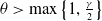 $\theta \gt \max \left \{1, \frac {\gamma }{2}\right \}$
. Then for
$\theta \gt \max \left \{1, \frac {\gamma }{2}\right \}$
. Then for $r\gt 1$
and for any
$r\gt 1$
and for any $T\gt 0$
, there exists a constant
$T\gt 0$
, there exists a constant $C\gt 0$
such that
$C\gt 0$
such that
 \begin{equation} \left \|\partial _t u_\iota ^\theta \right \|_{L^1\left (0, T ;\left (W_0^{1, r}(\Omega )\right )^*\right )} \leqslant C \end{equation}
for any $\iota \gt 0$
.
$\iota \gt 0$
.
Proof. Let $\delta \in C_0^{\infty }(\Omega )$
be such that
$\delta \in C_0^{\infty }(\Omega )$
be such that $\|\delta \|_{W_0^{1, r}(\Omega )} \leqslant 1$
. We denote with
$\|\delta \|_{W_0^{1, r}(\Omega )} \leqslant 1$
. We denote with $C_{\infty , f}$
the
$C_{\infty , f}$
the $\iota$
-independent
$\iota$
-independent $L^{\infty }$
-bound of a generic function
$L^{\infty }$
-bound of a generic function $f$
. Multiply the first equation of (2.6) by
$f$
. Multiply the first equation of (2.6) by $u_\iota { }^{\theta -1}$
to get
$u_\iota { }^{\theta -1}$
to get
 \begin{align} \int _{\Omega }\left (\frac {d}{d t} u_{\iota }\right ) \cdot u_{\iota }^{\theta -1} \zeta d x =&\int _{\Omega } \nabla \cdot \left (G_{\iota }\left (u_{\iota }\right ) \nabla u_{\iota }\right ) \cdot u_{\iota }^{\theta -1} \zeta d x -x \int _{\Omega } \nabla \cdot \left (f\left (u_{\iota }\right ) \nabla c_{\iota }\right ) \cdot u_{\iota }^{\theta -1} \zeta d x \nonumber\\ & +\int _{\Omega } M\left (u_{\iota }\right ) \cdot u_{\iota }^{\theta -1} \zeta d x\nonumber\\ \leqslant & \left (\theta -1\right )\int _0^T \int _{\Omega }D_{\iota }\left (u_{\iota }\right ) u_{\iota }^{\theta -2}\left |\nabla u_{\iota }\right |^{2} \cdot \left | \zeta \right | d x d t +\int _0^T \int _{\Omega } m_{\iota }^{\theta -1}\left | U\left (u_{\iota }\right )\cdot \zeta \right | d x d t \nonumber\\ & +\int _0^T \int _{\Omega }G_{\iota }\left (u_{\iota }\right ) u_{\iota }^{\theta -1} \left |\nabla u_{\iota } \cdot \nabla \zeta \right | d x d t + \chi \int _0^T \int _{\Omega } u_{\iota }^{\theta }\left |\nabla \eta _{\iota } \cdot \nabla \zeta \right | d x d t\nonumber\\ & +\chi (\theta -1) \int _0^T \int _{\Omega } u_{\iota }^{\theta -1}\left |\nabla \eta _{\iota } \cdot \nabla \eta _{\iota } \cdot \zeta \right | d x d t. \end{align}
For $T\gt 0$
, the density of
$T\gt 0$
, the density of $C_0^{\infty }(\Omega )$
in
$C_0^{\infty }(\Omega )$
in $W_0^{1, r}(\Omega )$
and an integration of the above equality in time, give
$W_0^{1, r}(\Omega )$
and an integration of the above equality in time, give
 \begin{align} \frac {1}{\theta }\left \|\partial _t u_\iota ^\theta \right \|_{L^1\left (0, T ;\left (W_0^{1, r}(\Omega )\right )^*\right )} \leqslant & (\theta -1) \int _0^T \int _{\Omega } u_\iota ^{\theta -2} \eta _\iota \left (u_\iota \right )\left |\nabla u_\iota \right |^2|\delta | \mathrm{d} x \mathrm{\,d} t \nonumber\\ & +\int _0^T \int _{\Omega } u_\iota ^{\theta -1} \eta _\iota \left (u_\iota \right )\left |\nabla u_\iota \cdot \nabla \delta \right | \mathrm{d} x \mathrm{\,d} t \nonumber\\ & +k_f \chi (\theta -1) \int _0^T \int _{\Omega } u_\iota ^{\theta -1}\left |\nabla u_\iota \cdot \nabla \eta _\iota \delta \right | \mathrm{d} x \mathrm{\,d} t \nonumber\\ & +k_f \chi \int _0^T \int _{\Omega } u_\iota ^\theta \left |\nabla \eta _\iota \cdot \nabla \delta \right | \mathrm{d} x \mathrm{\,d} t \nonumber\\ & +\int _0^T \int _{\Omega } u_\iota ^{\theta -1}\left |U\left (u_\iota \right ) \delta \right | \mathrm{d} x \mathrm{\,d} t. \end{align}
We now estimate each term on the r.h.s. separately. We start fixing $p\gt 1$
such that
$p\gt 1$
such that
 \begin{equation*} \theta \geqslant \max \left \{p, \frac {p+\gamma -1}{2}\right \}\!. \end{equation*}
In the subsequent analysis, we shall provide a detailed estimation of each individual component on the right-hand side of equation (5.3).
 \begin{align} \int _0^T \int _{\Omega } u_\iota { }^{\theta -2} \eta _\iota \left (u_\iota \right )\left |\nabla u_\iota \right |^2|\delta | \mathrm{d} x \mathrm{\,d} t & \leqslant C_{\infty , \delta } C_{\infty , u_\iota }^{\theta -p} \int _0^T \int _{\Omega } u_\iota { }^{p-2} \eta _\iota \left (u_\iota \right )\left |\nabla u_\iota \right |^2 \mathrm{\,d} x \mathrm{\,d} t \nonumber\\ & \leqslant C_{\infty , \delta } C_{\infty , u_\iota }^{\theta -p} C(1+T). \end{align}
The second term in (5.3) can be similarly estimated by Young’s inequality
 \begin{align} \int _0^T \int _{\Omega } u_\iota ^{\theta -1}G_\iota \left (u_\iota \right ) &\left |\nabla u_\iota \cdot \nabla \delta \right | d x d t \leqslant \int _0^T \int _{\Omega }G_\iota \left (u_\iota \right ) u_\iota ^{\theta -1}\left (\left |\nabla u_\iota \right |\right )d x d t \nonumber\\ &\leqslant \int _0^T \int _{\Omega }G_\iota \left (u_\iota \right ) u_\iota ^{\theta -1}\left (\frac {1}{2}\left |\nabla u_\iota \right |^2 + \frac {1}{2}\right )d x d t \nonumber\\ &\leqslant \frac {1}{4}C_{\infty ,\nabla \delta }C_{\infty ,G} C_{\infty ,u_\iota }^{2\theta -p-8+1}\int _0^T \int _{\Omega }u_\iota ^{\delta -1}\left | \nabla u_\iota \right |^2 d x d t+ \frac {1}{4}C_{\infty ,\nabla \delta }\cdot C(1+T)\nonumber\\ &+ \frac {1}{4}C_{\infty ,\nabla \delta }C_{\infty ,G} C_{\infty ,u_\iota }^{2\theta -p}\int _0^T \int _{\Omega }1 d x d t+ \frac {1}{4}C_{\infty ,\nabla \delta }C_{\infty ,G} C_{\infty ,u_\iota }^{p-2}\int _0^T \int _{\Omega }1 d x d t \nonumber\\ &\leqslant \frac {1}{4}C_{\infty ,\nabla \delta }C_{\infty ,G} C_{\infty ,u_\iota }^{2\theta -p-8+1}C(1+T)+\frac {1}{4}C_{\infty ,\nabla \delta }\cdot C(1+T)\nonumber\\ &+ \frac {1}{4}C_{\infty ,\nabla \delta }C_{\infty ,G} C_{\infty ,u_\iota }^{2\theta -p}T\left |\Omega \right |+ \frac {1}{4}C_{\infty ,\nabla \delta }C_{\infty ,G} C_{\infty ,u_\iota }^{p-2}T\left |\Omega \right |\!. \end{align}
The third equation of (5.3) can be written as
 \begin{align} \int _0^T \int _{\Omega } u_\iota ^{\theta -1}\left |\nabla u_\iota \cdot \nabla c_{\varepsilon } \cdot \delta \right | d x d t &\leqslant C_{\infty ,\delta }\int _0^T \int _{\Omega }u_\iota ^{\theta -1}\left |\nabla u_\iota \right |\left |\nabla \eta _\iota \right |d x d t\nonumber\\ &\leqslant \frac {1}{2}C_{\infty ,\delta }\int _0^T \int _{\Omega } u_\iota ^{2\theta -2}\left |\nabla u_\iota \right |^{2} d x d t+\frac {1}{2}\int _0^T \int _{\Omega }\left |\nabla \eta _\iota \right |^{2} d x d t\nonumber\\ &\leqslant \frac {1}{2}C_{\infty ,\delta } C_{\infty ,u_\iota }^{2\theta -p-8+1}\int _0^T \int _{\Omega }u_\iota ^{p+8-1}\left |\nabla u_\iota \right |^{2}d x d t+ \frac {1}{2}C_{\infty ,\delta } C_{\infty ,\nabla \eta _\iota }^{2}\cdot T\left |\Omega \right |\nonumber\\ &\leqslant \frac {1}{2}C_{\infty ,\delta } C_{\infty ,u_\iota }^{2\theta -p-8+1} C(1+T) + \frac {1}{2}C_{\infty ,\delta } C_{\infty ,\nabla \eta _\iota }^{2}T\left |\Omega \right |. \end{align}
Invoking again the bound for $\eta _\iota$
, we can easily bound
$\eta _\iota$
, we can easily bound
 \begin{equation} \int _0^T \int _{\Omega } u_\iota { }^\theta \left |\nabla \eta _\iota \cdot \nabla \delta \right | \mathrm{d} x \mathrm{\,d} t \leqslant C_{\infty , \nabla \delta } C_{\infty , u_\iota }^\theta C_{\infty , \nabla \eta _\iota }^2|\Omega | T. \end{equation}
Finally, it is easy to get
 \begin{equation} \int _0^T \int _{\Omega } u_\iota ^{\theta -1}\left |M\left (u_\iota \right ) \delta \right | \mathrm{d} x \mathrm{\,d} t \leqslant L C_{\infty , \delta } C_{\infty , u_\iota }^\theta (1+C_{\infty , u_\iota } )|\Omega | T. \end{equation}
Putting together (5.4)–(5.8), we can deduce the existence of a constant $C\gt 0$
independent on
$C\gt 0$
independent on $\iota$
such that (5.3) reduces to
$\iota$
such that (5.3) reduces to
 \begin{equation*} \left \|\partial _t u_\iota { }^\theta \right \|_{L^1\left (0, T ;\left (W_0^{1, r}(\Omega )\right )^*\right )} \leqslant C(1+T). \end{equation*}
Lemma 5.2.
Let $\chi \geqslant 0$
and
$\chi \geqslant 0$
and $\gamma$
under condition
$\gamma$
under condition $\gamma \gt \max \left \{2-\frac {2}{n}, 1\right \}$
for
$\gamma \gt \max \left \{2-\frac {2}{n}, 1\right \}$
for $n=1, 2, 3$
. For any
$n=1, 2, 3$
. For any $T \in (0, \infty ]$
, there exist
$T \in (0, \infty ]$
, there exist $c$
and
$c$
and $d$
belonging to
$d$
belonging to $L_{l o c}^2\left (0, T ;\, W^{1,2}(\Omega )\right ) \cap L^{\infty }(\Omega \times (0, T))$
and
$L_{l o c}^2\left (0, T ;\, W^{1,2}(\Omega )\right ) \cap L^{\infty }(\Omega \times (0, T))$
and $m \in L_{l o c}^2\left (0, T ;\, L^2(\Omega )\right ) \cap L^{\infty }(\Omega \times (0, T))$
such that, up to a non relabel sub-sequence,
$m \in L_{l o c}^2\left (0, T ;\, L^2(\Omega )\right ) \cap L^{\infty }(\Omega \times (0, T))$
such that, up to a non relabel sub-sequence,
 \begin{align} w_\iota \rightharpoonup c, \eta _\iota \rightharpoonup d & \text{ in } L_{l o c}^2\left (0, T ;\, L^2(\Omega )\right )\!, \end{align}
 \begin{align} w_\iota \stackrel {*}{\rightharpoonup } c, \eta _\iota \stackrel {*}{\rightharpoonup } d & \text{ in } L^{\infty }(\Omega \times (0, T)), \end{align}
 \begin{align} \nabla w_\iota \stackrel {*}{\rightharpoonup } \nabla c, & \text{ in } L^{\infty }(\Omega \times (0, T)), \end{align}
 \begin{align} u_\iota \rightarrow m & \text{ a.e. in } \Omega \times (0, T), \end{align}
 \begin{align} u_\iota \rightarrow m & \text{ in } L^2\left (0, T ;\, L^2(\Omega )\right )\!, \end{align}
 \begin{align} \eta _\iota \left (u_\iota \right ) \nabla u_\iota \rightharpoonup D(m) \nabla m & \text{ in } L^2\left (0, T ;\, L^2(\Omega )\right )\!, \end{align}
as $\iota \rightarrow 0$
.
$\iota \rightarrow 0$
.
Proof. The proof process relies heavily on key mathematical tools, including $L^{\infty }$
-estimates, the Aubin–Lions lemma [Reference Simon10], the principle of uniform bounded and Lebesgue’s dominated convergence theorem. These tools provide a robust theoretical framework that allows for the systematic analysis and derivation of the necessary mathematical results. To maintain the conciseness of the manuscript, the detailed steps of the proof are omitted here. However, it is anticipated that the introduction of the aforementioned methods offers readers a clear understanding of the underlying proof strategy. For those seeking a more thorough exploration, we recommend consulting the relevant literature for further details.
$L^{\infty }$
-estimates, the Aubin–Lions lemma [Reference Simon10], the principle of uniform bounded and Lebesgue’s dominated convergence theorem. These tools provide a robust theoretical framework that allows for the systematic analysis and derivation of the necessary mathematical results. To maintain the conciseness of the manuscript, the detailed steps of the proof are omitted here. However, it is anticipated that the introduction of the aforementioned methods offers readers a clear understanding of the underlying proof strategy. For those seeking a more thorough exploration, we recommend consulting the relevant literature for further details.
Then we can get the following theorem. The proof method is similar to that of [Reference Fagioli, Radici and Romagnoli21], so we will skip it here.
Theorem 5.1.
Let $\Omega \subset \mathbb{R}^n$
be a bounded domain with smooth boundary
$\Omega \subset \mathbb{R}^n$
be a bounded domain with smooth boundary $\partial \Omega$
and
$\partial \Omega$
and $\chi \gt 0$
. Assume that
$\chi \gt 0$
. Assume that $G$
satisfies
$G$
satisfies $\mathbf{(H1)}$
-
$\mathbf{(H1)}$
- $\mathbf{(H3)}$
. Consider a triple
$\mathbf{(H3)}$
. Consider a triple $\left (u_0, w_0, \eta _0\right )$
satisfying (
2.2
). Then, for any
$\left (u_0, w_0, \eta _0\right )$
satisfying (
2.2
). Then, for any $\gamma \gt 1$
that satisfies
$\gamma \gt 1$
that satisfies $\gamma \gt \max \left \{2-\frac {2}{n}, 1\right \}$
for
$\gamma \gt \max \left \{2-\frac {2}{n}, 1\right \}$
for $n=1, 2, 3$
, there is
$n=1, 2, 3$
, there is $C\gt 0$
such that system (
2.1
) has a weak solution
$C\gt 0$
such that system (
2.1
) has a weak solution $(u, w, \eta )$
that exists globally in time and satisfies
$(u, w, \eta )$
that exists globally in time and satisfies
 \begin{equation*} \|u(\cdot , t)\|_{L^{\infty }(\Omega )}+\|w(\cdot , t)\|_{W^{1, \infty }(\Omega )}+\|\eta (\cdot , t)\|_{W^{1, \infty }(\Omega )} \leqslant C \end{equation*}
for all $t \in (0, \infty )$
.
$t \in (0, \infty )$
.
6. Numerical simulation
In the previous part, we have carried out a theoretical analysis of the model and verified the existence and boundedness of the model solutions. In order to further explore the practical application value of the model, we assigned values to the parameters in the model and carried out numerical simulation in this part to intuitively understand the evolution law of population density and toxicant concentration.
(a) Evolution of population density $u$
with respect to time and space. (b) Heat map of population density
$u$
with respect to time and space. (b) Heat map of population density $u$
. (c) Evolution of toxicant
$u$
. (c) Evolution of toxicant $w$
with respect to time and space. (d) Heat map of toxicant
$w$
with respect to time and space. (d) Heat map of toxicant $w$
. (e) Evolution of cognitive ability
$w$
. (e) Evolution of cognitive ability $\eta$
with respect to time and space. (f) Heat map of cognitive ability
$\eta$
with respect to time and space. (f) Heat map of cognitive ability $\eta$
.
$\eta$
.
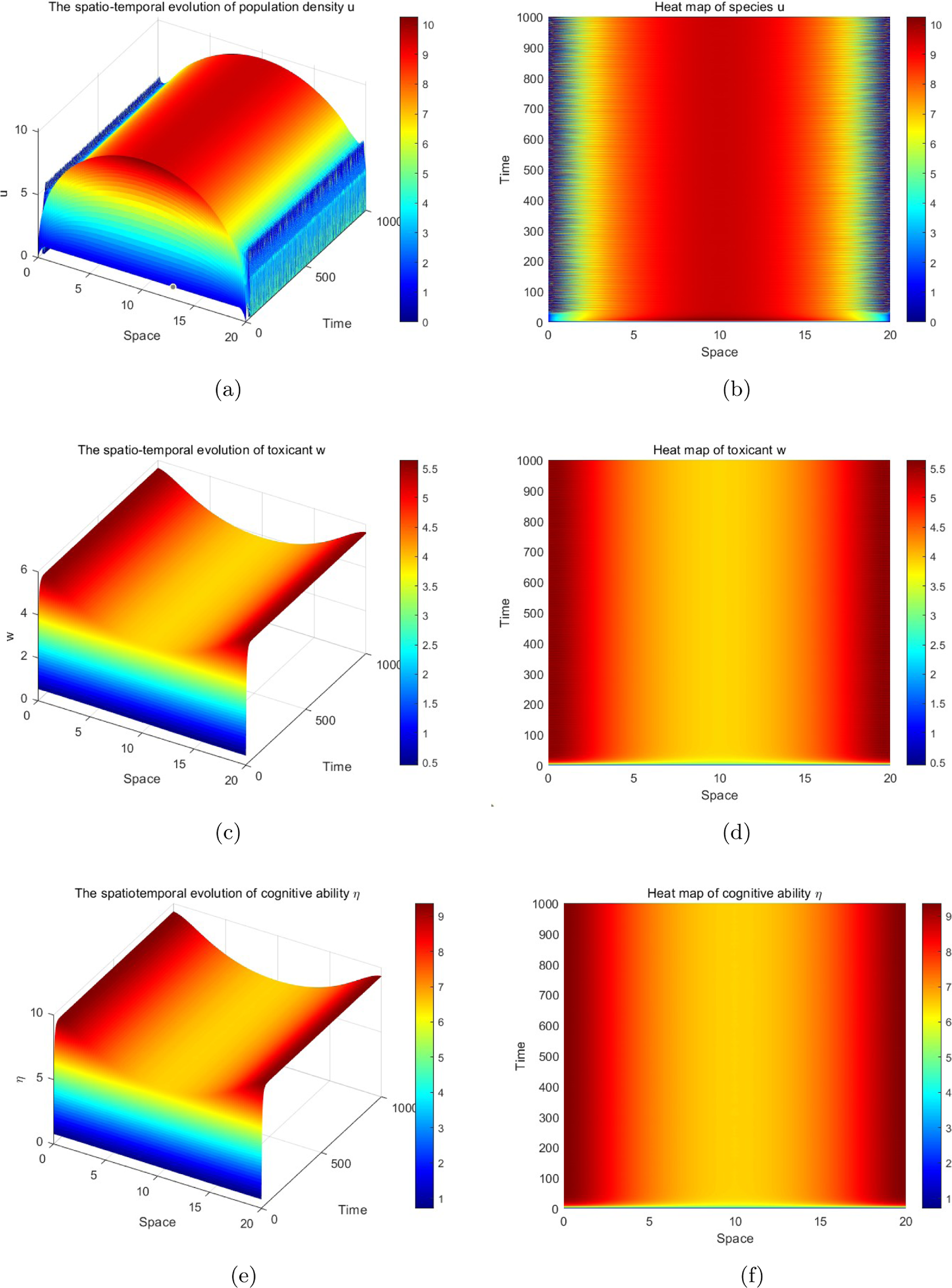
Figure 1. Long description
The image contains six graphs. The first graph (a) is a 3D surface plot showing the evolution of population density with respect to time and space. The second graph (b) is a heat map of population density, with time on the y-axis and space on the x-axis. The third graph (c) is a 3D surface plot showing the evolution of toxicant with respect to time and space. The fourth graph (d) is a heat map of toxicant, with time on the y-axis and space on the x-axis. The fifth graph (e) is a 3D surface plot showing the evolution of cognitive ability with respect to time and space. The sixth graph (f) is a heat map of cognitive ability, with time on the y-axis and space on the x-axis. Each heat map uses a color gradient to represent different values, with the color bar on the right indicating the scale. The 3D surface plots provide a visual representation of how each variable changes over time and space, while the heat maps offer a more detailed view of the distribution of these variables.
In Figure 1, we simulate the variation laws of population density and toxin concentration in a one-dimensional case. Figures (a), (c) and (e) are, respectively, the spatiotemporal evolution graphs of population concentration, toxin concentration and cognitive ability. Figures (b), (d) and (f) are the heat maps of population concentration, toxin concentration and cognitive ability, respectively. We clearly observe from Figures (c)–(f) the synchronicity of toxic substance concentration and cognitive ability: In the spatio-temporal evolution diagram, the phases of the two remain highly consistent, and in the heat map, their spatial distribution patterns are also closely connected. This synchronization phenomenon may stem from the feedback regulation mechanism of cognitive ability to toxic substance sensitivity, that is, organisms adjust their spatial distribution strategies by perceiving environmental toxicity.
It is worth noting that in sharp contrast to the above-mentioned synchronous phenomena, the evolution characteristics of population concentrations (Figures (a) and (b)) exhibit completely opposite behavioural patterns: when Figures (a) and (b) show the population aggregation areas, corresponding to Figures (c) and (d), they present the characteristics of toxin concentration dissipation. This reverse response mechanism may reflect the survival strategy of the population in a toxic environment. That is, when the concentration of toxic substances increases, the population reduces the exposure risk through active diffusion, thereby resulting in a decrease in the apparent distribution density (see Figure 1).
(a) Three-dimensional distribution of population density $u$
. (b) Contour lines of population density
$u$
. (b) Contour lines of population density $u$
. (c) Three-dimensional distribution of toxicant
$u$
. (c) Three-dimensional distribution of toxicant $w$
. (d) Contour lines of toxicant
$w$
. (d) Contour lines of toxicant $w$
. (e) Three-dimensional distribution of cognitive ability
$w$
. (e) Three-dimensional distribution of cognitive ability $\eta$
. (f) Contour lines of cognitive ability
$\eta$
. (f) Contour lines of cognitive ability $\eta$
.
$\eta$
.
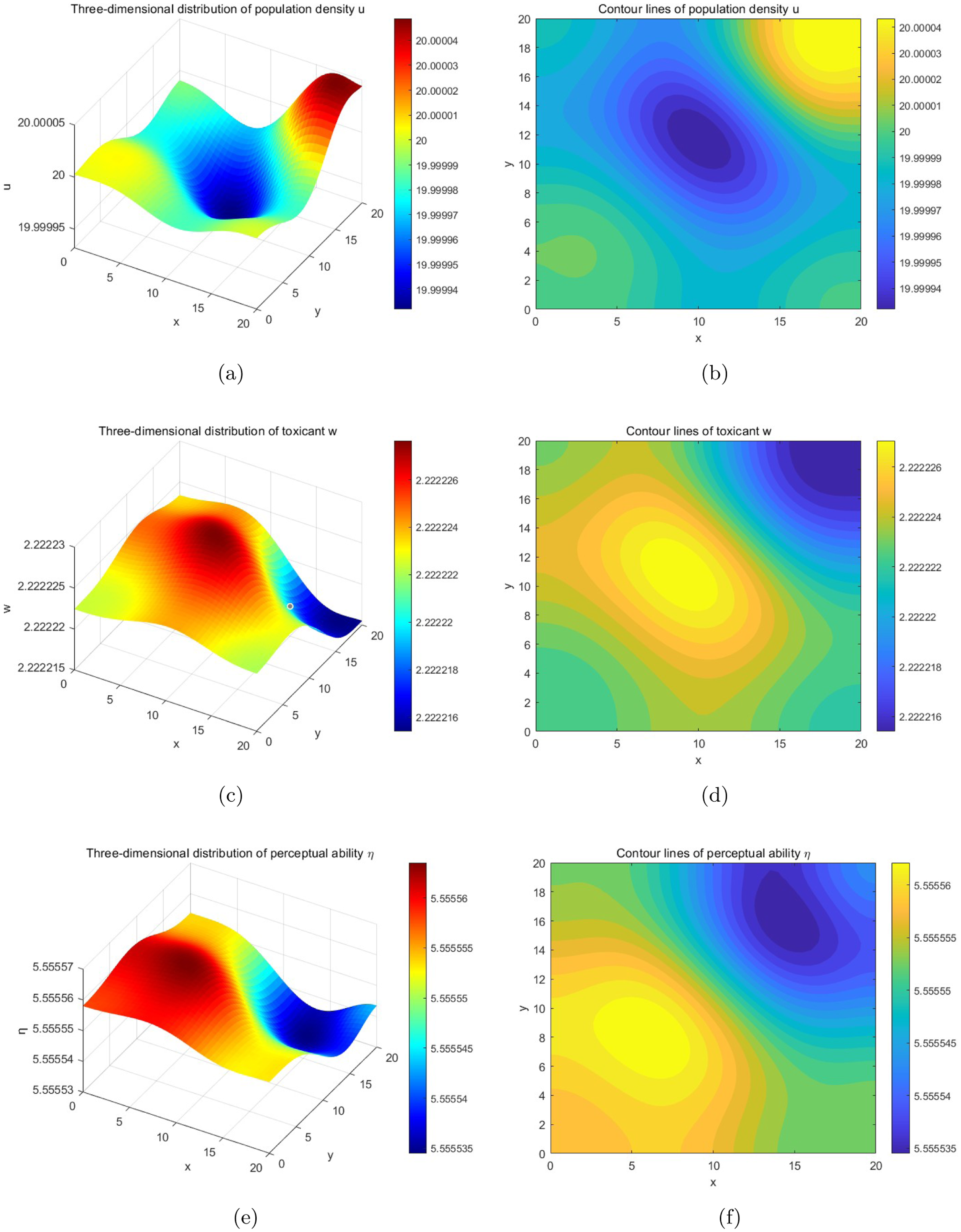
Figure 2. Long description
The image contains six subplots arranged in two rows and three columns. The first row shows three-dimensional distributions: population density, toxicant distribution, and cognitive ability. The second row displays corresponding contour lines for each distribution. Each subplot includes a color gradient to represent different values. The x and y axes in each subplot range from 0 to 20, and the z-axis in the three-dimensional plots ranges from specific minimum to maximum values. The contour lines in the second row provide a two-dimensional representation of the data shown in the three-dimensional plots above them. All values are approximated.
(a) Population density gradient field $\nabla u$
. (b) Toxicant gradient field
$\nabla u$
. (b) Toxicant gradient field $\nabla w$
. (c) Cognitive ability gradient field
$\nabla w$
. (c) Cognitive ability gradient field $\nabla \eta$
. (d) The phase space trajectory of the central point.
$\nabla \eta$
. (d) The phase space trajectory of the central point.
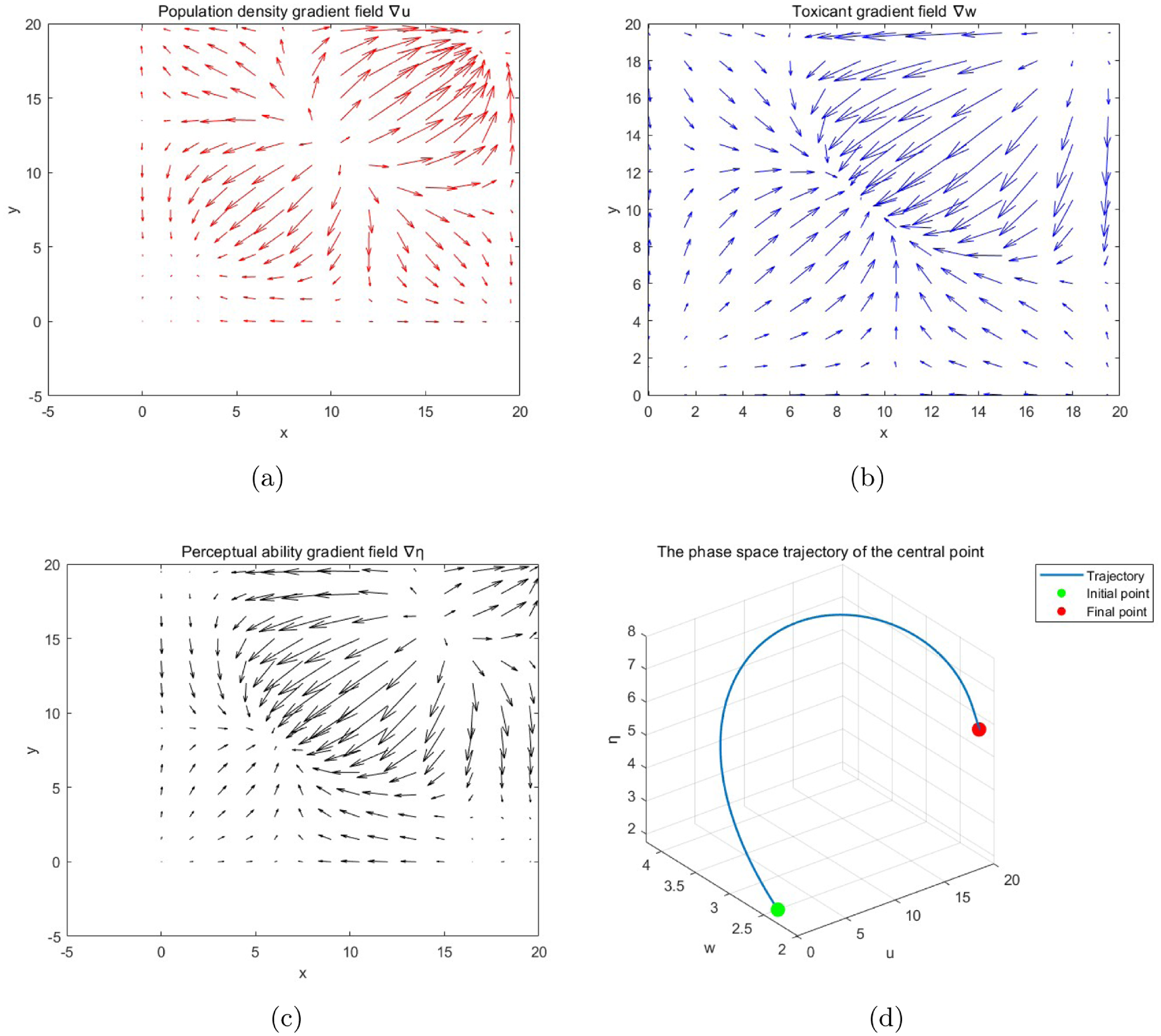
Figure 3. Long description
The image contains four separate graphs. The first graph, labeled (a), displays the population density gradient field with red arrows indicating the direction and magnitude of the gradient. The second graph, labeled (b), shows the toxicant gradient field with blue arrows. The third graph, labeled (c), represents the perceptual ability gradient field with black arrows. The fourth graph, labeled (d), illustrates the phase space trajectory of the central point in a 3D space with a blue line indicating the trajectory, a green dot marking the initial point, and a red dot marking the final point.
In Figures 2 and 3, we study the evolution and distribution patterns of population density, toxin concentration and cognitive ability through two-dimensional numerical simulation. Figure 2 shows the three-dimensional evolution and its corresponding contour map. The results indicate that the three variables all present uniform distribution characteristics in the vertical direction, which confirms that the system has reached the positive equilibrium state predicted by theory. Through quantitative analysis of the density of contour lines, we further discover that population density and toxic substance concentration exhibit obvious migration behaviours on the horizontal plane: the population tends to avoid areas with high toxic substance concentration, forming a specific spatial distribution pattern.
Figure 3(a)–(c) mainly presents the gradient field distribution of each variable. We find that the gradient direction of the population density ( $\nabla u$
) showed a significant negative correlation with the gradient of the toxic substance concentration (
$\nabla u$
) showed a significant negative correlation with the gradient of the toxic substance concentration ( $\nabla w$
), indicating that the population would actively avoid the areas where the toxic substance concentration increased. Meanwhile, we find that the gradient direction of cognitive ability (
$\nabla w$
), indicating that the population would actively avoid the areas where the toxic substance concentration increased. Meanwhile, we find that the gradient direction of cognitive ability ( $\nabla \eta$
) was highly consistent with the gradient of toxic concentration, indicating that organisms can accurately perceive toxic threats in the environment. The differences in this chemotactic behaviour reveal the inherent regulatory mechanism of the system: cognitive ability, as a mediating variable, achieves self-protection by guiding the population away from the toxic area, thereby maintaining the dynamic balance of the ecosystem. In Figure 3(d), we simulate the trajectory map of the phase space and find that the system has a steady-state attractor, indicating that at this time, the population density, toxin concentration and cognitive ability have reached a dynamic equilibrium.
$\nabla \eta$
) was highly consistent with the gradient of toxic concentration, indicating that organisms can accurately perceive toxic threats in the environment. The differences in this chemotactic behaviour reveal the inherent regulatory mechanism of the system: cognitive ability, as a mediating variable, achieves self-protection by guiding the population away from the toxic area, thereby maintaining the dynamic balance of the ecosystem. In Figure 3(d), we simulate the trajectory map of the phase space and find that the system has a steady-state attractor, indicating that at this time, the population density, toxin concentration and cognitive ability have reached a dynamic equilibrium.
These findings not only verify the biological rationality of the chemotactic term $\left (\chi \nabla \cdot \left (u \nabla \eta \right )\right )$
in the theoretical model, but more importantly, reveal the adaptive mechanism in the multi-factor coupled system: when environmental toxicity increases, organisms optimize the spatial distribution strategy by enhancing local cognitive ability. This result provides a new theoretical basis for understanding the regulation of population behaviour in complex ecological environments.
$\left (\chi \nabla \cdot \left (u \nabla \eta \right )\right )$
in the theoretical model, but more importantly, reveal the adaptive mechanism in the multi-factor coupled system: when environmental toxicity increases, organisms optimize the spatial distribution strategy by enhancing local cognitive ability. This result provides a new theoretical basis for understanding the regulation of population behaviour in complex ecological environments.
7. Discussion
This study establishes a single-species cognitive model with nonlinear degenerate diffusion and systematically investigates the population dynamics in a toxic environment.
In terms of theoretical analysis, we first prove the local existence of weak solutions to the model. Subsequently, via a regularization approach, we establish the global existence and uniform boundedness of classical solutions for the regularized system. Furthermore, through compactness arguments, we obtain the global existence of weak solutions for the original degenerate system, laying a rigorous mathematical foundation for the model.
In the numerical simulation part, we conduct studies for both one-dimensional and two-dimensional cases. The numerical results not only verify the reasonableness of the degenerate diffusion term and the coupling structure but also visually reveal the dynamic relationships among population density, toxin concentration and cognitive ability in spatiotemporal evolution. In particular, we observe a significant positive correlation between the cognitive gradient ( $\nabla \eta$
) and the toxin concentration gradient (
$\nabla \eta$
) and the toxin concentration gradient ( $\nabla w$
), while the population density gradient (
$\nabla w$
), while the population density gradient ( $\nabla u$
) exhibits the opposite trend. This phenomenon confirms that cognitive ability serves as a key regulatory mechanism for populations to actively avoid environmental risks.
$\nabla u$
) exhibits the opposite trend. This phenomenon confirms that cognitive ability serves as a key regulatory mechanism for populations to actively avoid environmental risks.
The theoretical results (global existence of weak solutions) provide fundamental mathematical assurance for analyzing such ‘cognitive-toxin’ coupled systems, and the framework can be extended to more general nonlinear diffusion terms or cognitive feedback mechanisms. However, the work still has certain limitations: First, the model assumes a linear cognitive memory process ( $\eta _t = bw - \gamma \eta$
) and a constant toxin input rate; future work could consider more complex nonlinear cognitive functions or time-varying environments. Second, the theoretical analysis requires the diffusion exponent to satisfy
$\eta _t = bw - \gamma \eta$
) and a constant toxin input rate; future work could consider more complex nonlinear cognitive functions or time-varying environments. Second, the theoretical analysis requires the diffusion exponent to satisfy $\gamma \gt \max \{2-2/n, 1\}$
; the solution properties for
$\gamma \gt \max \{2-2/n, 1\}$
; the solution properties for $\gamma$
below this critical threshold remain to be explored. Additionally, this paper does not address the uniqueness, stability or long-time asymptotic behaviour (e.g., formation of steady-state patterns) of the solutions.
$\gamma$
below this critical threshold remain to be explored. Additionally, this paper does not address the uniqueness, stability or long-time asymptotic behaviour (e.g., formation of steady-state patterns) of the solutions.
The observed phenomenon of ‘avoidance’ of space – that is, the population density in highly toxic areas decreases – is directly driven by the cognitive chemotactic term $\chi \nabla \cdot (u\nabla \eta )$
. This mechanism suggests that increasing the cognitive learning rate can enhance the population’s ability to avoid toxins. The parameter
$\chi \nabla \cdot (u\nabla \eta )$
. This mechanism suggests that increasing the cognitive learning rate can enhance the population’s ability to avoid toxins. The parameter $b$
, which increases
$b$
, which increases $\eta$
and its gradient, can theoretically enhance the population’s ability to escape from toxic areas, thereby potentially increasing its long-term survival probability. However, systematic parameter sensitivity analysis (which is left for future work) is still needed to quantify this effect and determine the critical threshold for the persistence of the population.
$\eta$
and its gradient, can theoretically enhance the population’s ability to escape from toxic areas, thereby potentially increasing its long-term survival probability. However, systematic parameter sensitivity analysis (which is left for future work) is still needed to quantify this effect and determine the critical threshold for the persistence of the population.
In summary, by combining theoretical analysis and numerical simulation, this study not only refines the theoretical framework for chemotaxis (cognitive-taxis) models with nonlinear diffusion but also provides new insights and modelling tools for understanding adaptive strategies of organisms in stressful environments.
Data availability statement
Not applicable.
Author contributions
Xinyu Bo: Formal analysis, methodology, software, writing – review and editing, writing – original draft; Wenjun Liu: methodology, supervision; Guangying Lv: methodology, supervision, formal analysis, writing – review and editing; Xuebing Zhang: methodology, software, writing – review and editing.
Funding statement
This work was supported by NSFC of China grants 12171247 and the Startup Foundation for Introducing Talent of NUIST.
Competing interests
The authors declare that they have no competing interests.
Ethical standards
Not applicable.


 u
u u
u w
w w
w η
η η
η
 u
u u
u w
w w
w η
η η
η
 ∇u
∇u ∇w
∇w ∇η
∇η
 Open access

