


INTRODUCTION
Increased ice-mass loss through melt and accelerated glacier discharge into the ocean has been observed in the Canadian Arctic and Greenland (e.g. Enderlin and others, Reference Enderlin2014; Harig and Simons, Reference Harig and Simons2016). A distinction has been made between the dynamic response of land-terminating and tidewater-terminating outlet glaciers (e.g. Joughin and others, Reference Joughin2008), whereby increases in ice velocity on land-terminating glaciers are often interpreted as hydraulically-driven sliding. Observational evidence from Arctic glaciers (e.g. Müller and Iken, Reference Müller and Iken1973; Bingham and others, Reference Bingham, Nienow and Sharp2003, Reference Bingham, Hubbard, Nienow and Sharp2008) and the Greenland ice sheet (e.g. Shepherd and others, Reference Shepherd2009; Bartholomew and others, Reference Bartholomew2010; Palmer and others, Reference Palmer, Shepherd, Nienow and Joughin2011) has linked seasonal and diurnal speed-up to surface meltwater production. However, this simple mechanism of melt-induced speed-up is nuanced when consideration is given to the response of the subglacial drainage system to variable meltwater input. High water fluxes may actually inhibit glacier acceleration (e.g. Sundal and others, Reference Sundal2011; Andrews and others, Reference Andrews2014) due to reductions in basal water pressure in response to the establishment of efficient subglacial drainage channels. Melt supply variability and drainage system capacity therefore play important roles in controlling any ice flow acceleration (Kavanaugh and others, Reference Kavanaugh, Moore, Dow and Sanders2010; Schoof, Reference Schoof2010).
Additional processes are at work on tidewater outlet glaciers, where dynamic changes are thought to be triggered primarily by perturbations at the ice/ocean interface (e.g. Nick and others, Reference Nick, Vieli, Howat and Joughin2009; Murray and others, Reference Murray2010, Reference Murray2015). For example, subglacial discharge (e.g. Beaird and others, Reference Beaird, Straneo and Jenkins2015; Fried and others, Reference Fried2015; Carroll and others, Reference Carroll2016) and warm waters entering fjords (e.g. Holland and others, Reference Holland, Thomas, Young and Ribergaard2008; Mortensen and others, Reference Mortensen, Lennert, Bendtsen and Rysgaard2011; Straneo and others, Reference Straneo2012) can thermally erode the submarine portion of the calving front, thereby changing the stress balance of the terminus region. Short-term velocity fluctuations in marine-terminating glaciers may also correlate with the break-up of frontal ice mélange (e.g. Amundson and others, Reference Amundson, Fahnestock, Truffer, Brown and Lüthi2010; Howat and others, Reference Howat, Box, Ahn, Herrington and McFadden2010; Walter and others, Reference Walter2012) and tidal forcing (e.g. Walters and Dunlap, Reference Walters and Dunlap1987; O'Neel and others, Reference O'Neel, Echelmeyer and Motyka2001).
This study addresses the dynamic response of a major Arctic tidewater glacier to seasonal and sub-seasonal changes. The outlet glacier has a scientific history dating back to 1961 (Boon and others, Reference Boon, Burgess, Koerner and Sharp2010) and was chosen for an in-depth investigation during the 2007/08 International Polar Year. Belcher Glacier (75°39′N; 81°30′W) is situated in the northeast sector of Devon Ice Cap in the Canadian Arctic (Fig. 1). It is the largest and fastest flowing outlet of Devon Ice Cap, and is estimated to account for 42% of the ice cap's calving loss (Van Wychen and others, Reference Van Wychen2012) and ~15% of its total mass loss (Burgess and others, Reference Burgess, Sharp, Mair, Dowdeswell and Benham2005). The along-flow distance from the ice-cap divide to the marine terminus is >40 km, of which the lower 16 km are characterized by glacier bed elevations below sea level. The terminal ice cliff is ~250 m thick and thought to be lightly grounded.
Field location. (a) Canada with Devon Island boxed in red. (b) Devon Ice Cap on Devon Island, with Belcher Glacier boxed in blue. (c) Belcher Glacier and its supraglacial drainage sub-catchments, channels, lakes and locations of moulins. Base image: Landsat 7, August 2000, NASA Landsat Program.

The present study uses a hydrologically-coupled higher-order ice flow model (Pimentel and others, Reference Pimentel, Flowers and Schoof2010; Pimentel and Flowers, Reference Pimentel and Flowers2011) adapted to the Belcher Glacier system. We use the model to investigate intra-annual velocity variations observed in 2008 and 2009, and in particular to evaluate the relative importance of frontal buttressing versus basal lubrication as controls on ice dynamics.
OBSERVATIONAL AND DERIVED DATA
DEM
We constructed DEMs of the surface and bed of Belcher Glacier from multiple data sources. Surface elevations come from the SPIRIT DEMs, which are derived from SPOT HRS 5 images acquired on 20 August and 17 October 2007 (Korona and others, Reference Korona, Berthier, Bernard, Rémy and Thouvenot2009). We mapped ice thicknesses using 12.5 MHz ground penetrating radar (GPR) data collected in May 2007 and May 2008 (Fig. 2a), complemented by coincident GPS measurements of surface elevation and position. Additional ice-thickness data come from 100 MHz airborne radar surveys conducted in April 2000 by the Scott Polar Research Institute at Cambridge University (see Fig. 2b and Dowdeswell and others (Reference Dowdeswell, Benham, Gorman and Burgess2004)) and 150 MHz radar surveys in 2005 by the Center for Remote Sensing of Ice Sheets at the University of Kansas. We used these ice-thickness data with the ice-surface elevations to determine bed elevations. Prior to interpolating the data to produce a DEM of the glacier bed (on the same spatial grid as the surface DEM), we averaged all bed elevation data within 56 m of each grid point of the DEM. We used an adaptive Gaussian kernel to implement inverse-distance weighting of the data in the averaging of the bed data. We derived model parameters from an experimental semivariogram for use in a kriging algorithm to generate the final bed DEM. A Landsat 7 panchromatic image from 2000 was used to delineate bedrock outcrops, where interpolated surface- and bed elevations were constrained to be equal. Our DEM of ice thickness was obtained by subtracting the final bed DEM from the ice-surface DEM (Fig. 2c).
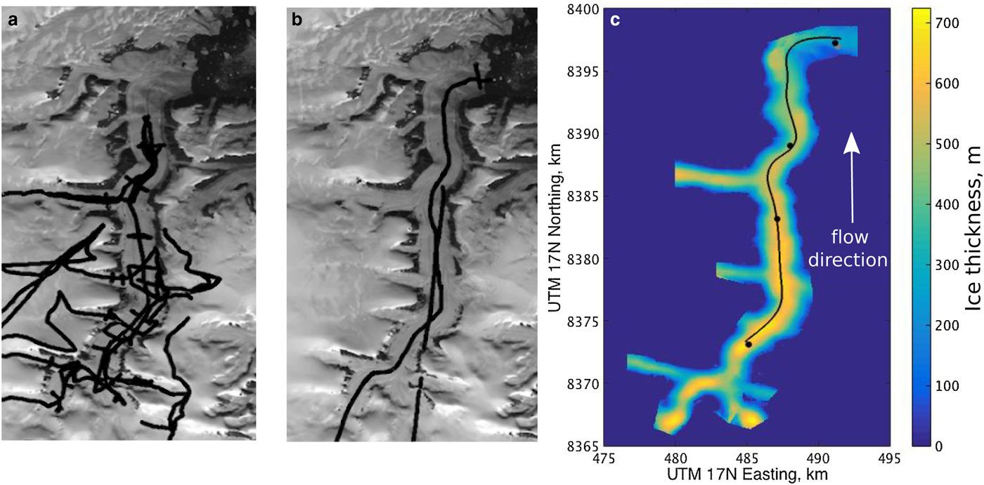
Radar survey locations and ice-thickness maps. (a) GPR survey (May 2007 and May 2008). (b) Airborne radar survey (April 2000, see Dowdeswell and others (Reference Dowdeswell, Benham, Gorman and Burgess2004)). (c) Belcher Glacier ice-thickness map annotated with flowline path (black line) and locations of GPS receivers (dots).
Surface velocities from GPS
We use continuous summer and partial over-winter GPS data from 2008 to 2010. Five Trimble NetRS dual-frequency GPS receivers were mounted on poles drilled into Belcher Glacier. From May through August of 2008 and 2009, the GPS receivers sampled at 15 s intervals. Data were processed using TRACK, the GAMIT kinematic processing software, to produce time series of position estimates at 30 s intervals (Danielson and Sharp, Reference Danielson and Sharp2013). For all of 2010, and September to April 2008 and 2009, the GPS receivers were programmed for a reduced duty cycle to extend operations. In this mode, data were collected at each GPS station for 1 hour at every 6 hours, and post-processed into a single position estimate using Precise Point Positioning (PPP). The resulting time series have one position estimate every 6 hours. This strategy allowed some of the stations to operate through the fall and early spring, though none operated during mid-winter (December–February).
Surface velocities from speckle tracking
We derived velocity maps of Belcher Glacier from various multi-day periods throughout 2009/10 using speckle tracking methods applied to Radarsat-2 imagery (Van Wychen and others, Reference Van Wychen2012). We extracted centreline profiles of ice-surface velocities along the main trunk glacier from maps of ice motion generated from satellite image pairs on the following dates: 1–25 March 2009, 5–29 March 2009, 3–27 October 2009, 21 December 2009–14 January 2010 and 8 February–3 March 2010. Error analysis of a subset of these data indicates an accuracy of
 ${\rm \sim} 5 \,{\rm ma}^{ - 1} $
when compared with the GPS-derived velocities at two of the GPS locations and
${\rm \sim} 5 \,{\rm ma}^{ - 1} $
when compared with the GPS-derived velocities at two of the GPS locations and
 ${\rm \sim} 10\! -\!\! 15\, {\rm ma}^{ - 1} $
when compared with a larger speckle-tracking dataset for locations over bedrock and at ice divides (Van Wychen and others, Reference Van Wychen2012).
${\rm \sim} 10\! -\!\! 15\, {\rm ma}^{ - 1} $
when compared with a larger speckle-tracking dataset for locations over bedrock and at ice divides (Van Wychen and others, Reference Van Wychen2012).
Surface run-off
We identified six surface runoff sub-catchments on the Belcher Glacier based on surface topography. Each sub-catchment contains supraglacial channels and lakes that were mapped using a combination of satellite imagery, aerial photography and field observations (Fig. 1c). We used a distributed surface energy-balance model coupled with a multi-layer, subsurface snow model to generate a time series of daily run-off for each sub-catchment for 2008 and 2009 (Duncan, Reference Duncan2011). The model was driven by on-ice meteorological data and validated with in situ field measurements of albedo, snow/ice ablation, and snowpack temperature and density. Run-off from each catchment feeds supraglacial meltwater channels that either drain into moulins or crevasses, or discharge into supraglacial lakes. The lakes eventually drain through a spillway or in situ through fracture propagation (e.g. Boon and Sharp (Reference Boon and Sharp2003)). We established the timing of lake drainage events and the opening of moulins by using time-lapse photography (see Danielson and Sharp (Reference Danielson and Sharp2013) for further details). For the purposes of the modelling, once these surface-to-bed connections are established, all subsequent run-off is assumed to drain directly to the bed at these locations.
Run-off from catchments 1, 2 and 3 initially accumulates in supraglacial lakes. On specific dates (determined from time-lapse photography), these lakes drain over the ice surface and into moulins. Run-off from catchment 4 accumulates in a supraglacial lake before rapid fracture-driven drainage occurs within the lake basin. Run-off from catchment five drains through crevasses, which are prevalent towards the terminus of the glacier. Run-off from catchment 6 is not thought to influence the dynamics of the glacier and so is not included in this study. The timing of the drainage events is given in Table 1, with a more complete analysis for 2009 provided by Danielson and Sharp (Reference Danielson and Sharp2013).
Timing of drainage events in each sub-catchment (see Fig. 1c)
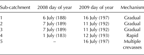
Drainage is classified as ‘gradual’ (supraglacial lake water transported by an incised surface channel to a downstream moulin) or ‘rapid’ (catastrophic lake drainage through a crevasse or moulin within the lake basin). Sub-catchment 5 drains through multiple crevasses near the glacier terminus.
COMPUTATIONAL MODEL
Below we provide an overview of the hydrologically coupled ice flow model, which is described in detail elsewhere (Pimentel and others, Reference Pimentel, Flowers and Schoof2010; Pimentel and Flowers, Reference Pimentel and Flowers2011) and has been used in previous work (Flowers and others, Reference Flowers, Roux, Pimentel and Schoof2011; Beaud and others, Reference Beaud, Flowers and Pimentel2014).
Ice flow
We use a ‘higher-order’ ice-dynamics model (Pattyn and others, Reference Pattyn2008) with the well-known Stokes-flow approximation (Blatter, Reference Blatter1995; Pattyn, Reference Pattyn2002) that retains second-order accuracy regardless of the amount of glacier slip (Schoof and Hindmarsh, Reference Schoof and Hindmarsh2010). Our particular version is 2-D in x (flowline direction) and z (vertical direction, between glacier bed, b, and ice surface, s), but approximates aspects of 3-D flow with a flow-band adaptation (channel half-width ω = ω(x, z)), and a lateral drag parameterization based on the velocity at the valley wall (u wall = u wall (x, z)). An elliptic problem for the horizontal velocity u = u(x,z) is solved by iterating on viscosity η = η(x, z):
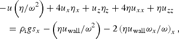 $$\eqalign{& -\! u\left( {\eta /\omega ^2} \right) + 4u_x \eta _x + u_z \eta _z + 4\eta u_{xx} + \eta u_{zz} \cr & \quad = \rho _{\rm i} gs_x - \left( {\eta u_{{\rm wall}} /\omega ^2} \right) - 2\left( {\eta u_{{\rm wall}} \omega _x /\omega} \right)_x,} $$
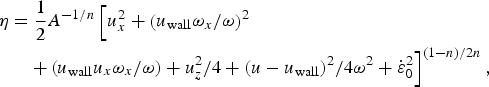 $$\eqalign{ \eta & = \displaystyle{1 \over 2}A^{ - 1/n} \left[ u_x^2 + \left( {u_{{\rm wall}} \omega _x /\omega} \right)^2 \right.\cr & \quad \left.+ \left( {u_{{\rm wall}} u_x \omega _x /\omega} \right) + u_z^2 /4 + (u - u_{{\rm wall}} )^2 /4\omega ^2 + \dot \varepsilon_0^2 \right]^{(1 - n)/2n},}$$
where subscripts t and x represent partial derivatives, i.e. u
x
= ∂u/∂x. Table 2 gives values of Glen's flow-law coefficient A and exponent n, ice density ρ
i, gravitational acceleration g, and the viscosity regularisation parameter
 $\dot {\rm \epsilon} _0 $
.
$\dot {\rm \epsilon} _0 $
.
Model constants and parameters

Boundary conditions
We use a regularized Coulomb friction law as a Robin-type boundary condition at the base of the glacier that relates basal drag τ b to sliding speed u b = u(x, z = b) (Schoof, Reference Schoof2005; Gagliardini and others, Reference Gagliardini, Cohen, Raback and Zwinger2007):
 $$\tau _{\rm b} = CN\left( {\displaystyle{{u_{\rm b}} \over {\Lambda C^n N^n + u_{\rm b}}}} \right)^{1/n}, $$
where Λ ∝ A (u
b = Λτ
b in the absence of cavitation) and the constant C represents a maximum for τ
b/N and satisfies ‘Iken's bound’, an upper bound requiring that C be less than or equal to the maximum bedrock slope (see Iken (Reference Iken1981); Schoof (Reference Schoof2005)). Eqn (3) is influenced by spatial and temporal variations in basal water pressure
 $P_{\rm w}^{\rm s} $
through the effective pressure
$P_{\rm w}^{\rm s} $
through the effective pressure
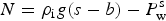 $N = \rho _{\rm i} g(s - b) - P_{\rm w}^{\rm s} $
. The friction law is similarly applied to the valley walls to obtain u
wall (see Pimentel and others (Reference Pimentel, Flowers and Schoof2010) for details).
$N = \rho _{\rm i} g(s - b) - P_{\rm w}^{\rm s} $
. The friction law is similarly applied to the valley walls to obtain u
wall (see Pimentel and others (Reference Pimentel, Flowers and Schoof2010) for details).
The ice/atmosphere interface is treated as a stress-free surface:
 $$s_x \left( {4u_x + 2u_{{\rm wall}} \omega _x /\omega} \right) - u_z = 0\quad {\rm at}\quad z = s.$$
The boundary condition at the calving front of a tidewater-terminating glacier adapted for backstress, σ B , is given by Nick and others (Reference Nick, van der Veen, Vieli and Benn2010). Here we also include δ t, a perturbation to sea-level due to tidal cycles (cf. (cf. Brunt and MacAyeal (Reference Brunt and MacAyeal2014)):
 $$U_x = A\left[ {\displaystyle{{\rho _{\rm i} g} \over 4}\left( {h - \displaystyle{{\rho _{\rm s}} \over {\rho _{\rm i} h}}\left( {\displaystyle{\rho \over {\rho _{\rm s}}} h} \right)^2 - \delta _{\rm t} - \displaystyle{{\sigma _B} \over {\rho _{\rm i} g}}} \right)} \right]^n, $$
where U x is the vertically integrated horizontal strain rate, h is the ice thickness at the terminus and ρ s is the density of seawater. For our purposes, σ B represents the backstress exerted by processes at the glacier terminus such as the effects of changing ice-mélange conditions. Belcher Glacier's terminus position is relatively stable (Burgess and others, Reference Burgess, Sharp, Mair, Dowdeswell and Benham2005), so we do not consider an evolving frontal position in this study and adopt a calving rule that maintains a constant ice thickness at the ice/ocean interface.
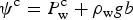
Hydrologic coupling
Spatial and temporal variations in basal water pressure are modelled using interacting inefficient and efficient subglacial drainage systems. The model used here is detailed in Pimentel and Flowers (Reference Pimentel and Flowers2011) and contextualized with respect to other drainage models in Flowers (Reference Flowers2015). The inefficient system is modelled as a macro-porous water sheet with an area-averaged thickness h
s, basal water pressure
 $P_{\rm w}^{\rm s} $
, water flux q
s and fluid potential
$P_{\rm w}^{\rm s} $
, water flux q
s and fluid potential
 $\psi ^{\rm s} = P_{\rm w}^{\rm s} + \rho _{\rm w} gb$
:
$\psi ^{\rm s} = P_{\rm w}^{\rm s} + \rho _{\rm w} gb$
:
 $$h_t^{\rm s} + q_x^{\rm s} = (Q_{\rm G} + u_{\rm b} \tau _{\rm b} )/\rho _{\rm i} L + \dot b^{\rm s} + \phi ^{{\rm s:c}}, $$
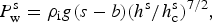 $$P_{\rm w}^{\rm s} = \rho _{\rm i} g(s - b)(h^{\rm s} /h_{\rm c}^{\rm s} )^{7/2}, $$
 $$q^{\rm s} = - Kh^{\rm s} \psi _x^{\rm s} /\rho _{\rm w} g,$$
where
 $\dot b^{\rm s} $
is the meltwater source term for the inefficient system and ϕ
s:c denotes the water exchange between inefficient and efficient drainage systems (see Eqn (12)). The effective hydraulic conductivity, K, varies as a function of h
s = h
s(x, t) and has a median value of
$\dot b^{\rm s} $
is the meltwater source term for the inefficient system and ϕ
s:c denotes the water exchange between inefficient and efficient drainage systems (see Eqn (12)). The effective hydraulic conductivity, K, varies as a function of h
s = h
s(x, t) and has a median value of
 $0.4 \,{\rm ms}^{ - 1} $
in this study. Table 2 gives values for the geothermal flux Q
G, the latent heat of fusion L, the critical sheet thickness
$0.4 \,{\rm ms}^{ - 1} $
in this study. Table 2 gives values for the geothermal flux Q
G, the latent heat of fusion L, the critical sheet thickness
 $h_{\rm c}^{\rm s} $
and the density of water ρ
w.
$h_{\rm c}^{\rm s} $
and the density of water ρ
w.
The efficient system is modelled as a semi-circular bed-floored, water-filled Röthlisberger channel with cross-sectional area S, water pressure
 $P_{\rm w}^{\rm c} $
, water discharge Q
c and fluid potential
$P_{\rm w}^{\rm c} $
, water discharge Q
c and fluid potential
 $\psi ^{\rm c} = P_{\rm w}^{\rm c} + \rho _{\rm w} gb$
:
$\psi ^{\rm c} = P_{\rm w}^{\rm c} + \rho _{\rm w} gb$
:
 $$\eqalign{& S_t + Q^{\rm c} (\psi _x^{\rm c} - c_{\rm p} \rho _{\rm w} \Phi P_{{\rm w},x}^{\rm c} )/\rho _{\rm i} L \cr & \quad = 2AS(\rho _{\rm i} g(s - b) - P_{\rm w}^{\rm c} )^n /n^n,}$$
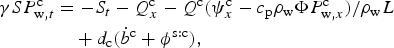 $$\eqalign{\gamma SP_{{\rm w},t}^{\rm c} & = - S_t - Q_x^{\rm c} - Q^{\rm c} (\psi _x^{\rm c} - c_{\rm p} \rho _{\rm w} \Phi P_{{\rm w},x}^{\rm c} )/\rho _{\rm w} L \cr & \quad + d_{\rm c} (\dot b^{\rm c} + \phi ^{{\rm s:c}} ),}$$
 $$Q^{\rm c} = - 2\sqrt 2 \psi _x^{\rm c} S^{3/2} /(P_{{\rm wet}} \rho _{\rm w} f_{\rm R} \vert \psi _x^{\rm c} \vert )^{1/2}. $$
Here
 $\dot b^{\rm c} $
denotes the meltwater source term to the efficient system, P
wet is the perimeter of S and f
R
is a friction coefficient given by
$\dot b^{\rm c} $
denotes the meltwater source term to the efficient system, P
wet is the perimeter of S and f
R
is a friction coefficient given by
 $f_{\rm R} = 8gn'^2 R_{\rm H}^{ - 1/3} $
with hydraulic radius R
H = S/P
wet. The latent conduit spacing, d
c, is set equal to the glacier width based on time-lapse photography at the terminus indicating a single primary meltwater plume. Table 2 gives values for the Manning roughness n′, specific heat capacity of water c
p, numerical compressibility γ and Clausius–Clapeyron slope Φ.
$f_{\rm R} = 8gn'^2 R_{\rm H}^{ - 1/3} $
with hydraulic radius R
H = S/P
wet. The latent conduit spacing, d
c, is set equal to the glacier width based on time-lapse photography at the terminus indicating a single primary meltwater plume. Table 2 gives values for the Manning roughness n′, specific heat capacity of water c
p, numerical compressibility γ and Clausius–Clapeyron slope Φ.
The rate of water exchange between the efficient and inefficient subglacial drainage systems is modelled as (Flowers, Reference Flowers2008):
 $$\phi ^{{\rm s:c}} = \chi ^{{\rm s:c}} \displaystyle{{Kh^{{\rm s:c}}} \over {\rho _{\rm w} gd_{\rm c}^2}} (P_{\rm w}^{\rm s} - P_{\rm w}^{\rm c} ),$$
where χ
s:c is a fixed coefficient (Table 2) and h
s:c is found by solving Eqn (7) with the left-hand side set to
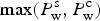 $\max (P_{\rm w}^{\rm s}, P_{\rm w}^{\rm c} )$
.
$\max (P_{\rm w}^{\rm s}, P_{\rm w}^{\rm c} )$
.
MODEL APPLICATION TO THE BELCHER GLACIER SYSTEM
The Belcher Glacier system (Fig. 1c) consists of a main trunk glacier formed from four convergent tributary glaciers. Approximately half way to its terminus, a major tributary joins the trunk glacier on its western side. A further six minor tributaries feed the trunk glacier upstream of this major tributary junction. Approximately 6 km from the marine terminus, the Belcher Glacier merges with another major tributary that enters from the west. Maximum velocities are observed near the centreline of the main Belcher Glacier, thus the flowline dynamics do not appear strongly influenced by this near-terminus confluence (Van Wychen and others, Reference Van Wychen2012). We therefore exclude this final tributary from the model.
Glacier flowline and tributary fluxes
The centreline profile location is shown in Figure 2c and the corresponding profiles of surface- and bed elevation in Figure 3a. The modelled flowline begins just downstream of the four convergent tributaries at the head of the glacier (see Fig. 2c). The ice-surface velocity at this location has been determined from annual (May 2008–May 2009) GPS displacement measurements to be
 $56\, {\rm ma}^{ - 1} $
. The upstream boundary condition on the ice flow model is prescribed by computing the vertical velocity profile using the shallow-ice equation and then scaling this profile based on the measured GPS surface velocity at this location. Surface velocities at the upstream boundary are thus constrained to match the GPS time series. At the downstream end of the flowline, the terminus position is held fixed at the marine boundary. Observations suggest that the annual mean terminus position has been stable for at least 50 years (Burgess and others, Reference Burgess, Sharp, Mair, Dowdeswell and Benham2005) with a range in annual minimum positions of ~375 m between 1999 and 2010. Time-lapse photography and Landsat 7 images from 2009 indicate minimal seasonal variability of the terminus position. Motion, where it occurs, is largely concentrated in the southern portion of the terminus away from the centreline, where the change in position of the ice margin was <290 m horizontal grid resolution of the model.
$56\, {\rm ma}^{ - 1} $
. The upstream boundary condition on the ice flow model is prescribed by computing the vertical velocity profile using the shallow-ice equation and then scaling this profile based on the measured GPS surface velocity at this location. Surface velocities at the upstream boundary are thus constrained to match the GPS time series. At the downstream end of the flowline, the terminus position is held fixed at the marine boundary. Observations suggest that the annual mean terminus position has been stable for at least 50 years (Burgess and others, Reference Burgess, Sharp, Mair, Dowdeswell and Benham2005) with a range in annual minimum positions of ~375 m between 1999 and 2010. Time-lapse photography and Landsat 7 images from 2009 indicate minimal seasonal variability of the terminus position. Motion, where it occurs, is largely concentrated in the southern portion of the terminus away from the centreline, where the change in position of the ice margin was <290 m horizontal grid resolution of the model.
Model representation of glacier geometry. Grey lines are the profiles from the DEMs and black lines are the profiles used in the model. (a) ice surface and bed elevations along flowline. (b) Surface width along flowline. (c) A representative glacier cross section.

Ice fluxes from the one major and six minor tributaries have been estimated by Van Wychen and others (Reference Van Wychen2012) based on remotely sensed surface velocities. These tributary fluxes are accounted for in the model by converting the ice flux into an equivalent surface mass-balance perturbation. The perturbations are then applied to the model grid points closest to the tributary junction locations, and act as source terms as the free surface evolves in time.
Channel shape
A cross-sectional profile of the glacier was calculated at each gridpoint along the flowline by dividing the surface width across the glacier (perpendicular to the flowline) into 30 equal intervals and determining the ice thickness in each interval using the surface and bed DEMs. The channel shape was found to be consistently parabolic along the flowline. A representative channel shape was then obtained by fitting a quadratic function to the mean of all the cross-sectional profiles after they were normalized to a unit width. This function, together with the observed variation in glacier width at the surface along the flowline, smoothed using a 4th-order polynomial (Fig. 3b), is used to approximate glacier width as a function of flow line position and depth, i.e. ω = ω(x, z) (see Fig. 3c for an example). Making use of the parabolic valley shape provides cross-sectional area estimates with a normalized RMS deviation of 5.6% from the areas derived from the elevation models. By contrast, if a rectangular-shaped channel is assumed, the cross-sectional area is grossly over-estimated, with a normalized RMS deviation of 34.1%. We set a minimum surface half-width of 250 m to prevent unbounded lateral drag in Eqn (1).
Glen's flow-law coefficient
Temperature measurements from deep boreholes at the summit of Devon Island Ice Cap indicate that the central ice cap is cold-based (Paterson, Reference Paterson1976), whereas the fast-flowing outlet glaciers are likely warm-based at their termini (Dowdeswell and others, Reference Dowdeswell, Benham, Gorman and Burgess2004). The ice near the bed, where most deformation occurs, may also be near the pressure melting point. However, without ice-temperature measurements or thermo-mechanical modelling for Belcher Glacier, we cannot accurately derive an ice-temperature field or values for the temperature-dependent rate factor, A, in Glen's flow law. With this restriction, we take a value of A corresponding to temperate ice (Cuffey and Paterson, Reference Cuffey and Paterson2010); this value represents an upper bound on ice-softness for this glacier. If the ice is colder, and therefore stiffer, the contribution of glacier sliding to surface velocities would be greater. Higher sliding rates would be achieved in the model by reducing parameter values Λ and/or C in the friction law.
Model spin-up and parameter tuning
To remove unwanted transients generated from non-equilibrium and irregular glacier geometry we apply the mean 1980–2006 annual net mass balance (Gardner and Sharp, Reference Gardner and Sharp2009), along with the tributary fluxes, to the Belcher flowline, while holding the terminus position fixed and allowing the free surface to evolve. Due to the negative mass balance of the glacier, no steady state could be found for these conditions. We therefore adopt a transient initial state that removes the initial perturbations in ice-surface elevation. A reference geometry (Fig. 3a) is thus established that smooths slope irregularities, while modelled ice-surface elevations and velocities remain close to observed values. Using this reference geometry enables us to examine the glacier response to melt-season forcing and boundary perturbations. The ‘spin-up’ simulation used to obtain the reference geometry employs a constant basal water-pressure distribution. This distribution was obtained a priori by running the subglacial drainage model, including only the inefficient system, to steady state; we thus obtain a baseline ‘winter’ water pressure distribution along the bed. We also assume no buttressing at the terminus (i.e. σ B = 0 in Eqn (5)).
We define a winter baseline velocity field using the steady-state ‘winter’ water-pressure distribution described above, under the assumption that the subglacial hydrologic system is reset to some steady-state condition in winter. Without a strong hydraulic stimulus in the form of surface melt, the glacier flows at a slower and steadier rate than it does in summer. This is likely an over-simplification of the actual subglacial conditions (cf. Schoof and others, Reference Schoof, Rada, Wilson, Flowers and Haseloff2014), but it serves as a basis for assessing the glacier's seasonal behaviour. The GPS-derived velocities for Belcher Glacier seem to largely support this idea, although there are some winter variations in ice velocities detected by Radarsat-2 speckle tracking (Van Wychen and others, Reference Van Wychen2012). Furthermore, we have observed fractured and collapsed lake ice on the basin floors in spring, suggesting the potential for delivery of supraglacial water to the bed during winter lake-drainage events.
Friction-law parameters
In the friction law (Eqn (3)) the parameters Λ and C can be related to the wavelength of the dominant bedrock bumps λ max, and the maximum bedrock slope m max, as follows: Λ ≈ kA, where A is Glen's flow-law coefficient and k = λ max/m max with C ≤ m max. Since these values are unknown, they are set using a sensitivity analysis in which we select a parameter pair (k,C) that minimizes differences between the modelled and observed ice-surface velocities.
Meltwater forcing
Using imagery from Landsat-7, Wyatt and Sharp (Reference Wyatt and Sharp2015) found that interannual velocity variability on Devon Ice Cap was greater in areas close to locations where surface drainage ended abruptly without re-establishment further down-glacier. This motivates our approach to delivering surface water to the basal drainage system in the model. Surface run-off in each sub-catchment is assumed to accumulate supraglacially until a surface-to-bed connection is established (with the exception of catchment 5 in 2008). Once a surface-to-bed connection exists (see Table 1), any stored water and all subsequent meltwater is fed directly into the modelled subglacial drainage system. The possibility of englacial transport and/or storage is not addressed. Exactly when and how the connection occurs depends on the individual catchment (see Table 1). The drainage entry point for meltwater from sub-catchment 1 occurs at the upstream boundary of the model domain, so meltwater input from this catchment drives a prescribed water-flux boundary condition (Eqn (6)). Meltwater from sub-catchments 2–4 enters the model at the grid point location closest to the draining lake or moulin, and is accommodated in the model initially through the (inefficient) sheet drainage system, via source term
 $\dot b^{\rm s} $
(Eqn (6)). Over a 24-hour period following the drainage event, meltwater input to the model transitions linearly to the (efficient) channelized drainage system, via source term
$\dot b^{\rm s} $
(Eqn (6)). Over a 24-hour period following the drainage event, meltwater input to the model transitions linearly to the (efficient) channelized drainage system, via source term
 $\dot b^{\rm c} $
(Eqn (10)). Sub-catchment 5 is heavily crevassed and Wyatt and Sharp (Reference Wyatt and Sharp2015) suggest that distributed drainage of surface meltwater through crevasses is the dominant mode of meltwater delivery to the bed in this region. We therefore prescribe uniform water input in this catchment to all grid points down-glacier of the lake (visible in Fig. 1c) through the source term
$\dot b^{\rm c} $
(Eqn (10)). Sub-catchment 5 is heavily crevassed and Wyatt and Sharp (Reference Wyatt and Sharp2015) suggest that distributed drainage of surface meltwater through crevasses is the dominant mode of meltwater delivery to the bed in this region. We therefore prescribe uniform water input in this catchment to all grid points down-glacier of the lake (visible in Fig. 1c) through the source term
 $\dot b^{\rm c} $
. Due to failure of the time-lapse photography equipment in 2008 we have no direct observations of lake drainage timing for sub-catchment 5, so we assume that a surface-to-bed connection is open from the onset of the melt season in 2008.
$\dot b^{\rm c} $
. Due to failure of the time-lapse photography equipment in 2008 we have no direct observations of lake drainage timing for sub-catchment 5, so we assume that a surface-to-bed connection is open from the onset of the melt season in 2008.
RESULTS
Winter baseline simulations
Modelled ice-surface speeds along the flowline are compared with both in situ and remotely-sensed data (Fig. 4a). The profile of modelled winter baseline speeds is broadly similar to the observations and falls within the range of measured winter flowline speeds. Differences are small when compared with the variability of observed melt-season flowspeeds, represented here by the minimum and maximum GPS-derived summer values (vertical bars, Fig. 4a). Further context on the seasonal range of observed ice-surface velocities is provided in Figure 4c.
Modelled and measured ice-surface speeds. (a) Modelled speeds along the Belcher Glacier centreline with sea-ice backstresses of 0 and 150 kPa are shown as black lines. Observed centreline speeds from Radarsat-2 speckle tracking are shown as coloured lines. Grey (2008) and black (2009) vertical bars indicate the summer minimum and maximum speeds computed from GPS-derived 24-hr running means. GPS-derived winter baseline speeds are shown as dots. (b) Modelled surface speeds at the terminus from different backstress perturbations: no perturbation (black star and dashed line), sea-ice backstress (blue crosses), and tidal sea-level change (red dots). (c) A time series of observed speeds. GPS-derived 24-hr running means are shown as coloured lines according to station location given as distance from the glacier terminus. Horizontal bars indicate observed centreline speeds from Radarsat-2 speckle tracking, colour indicates distance from the glacier terminus.

Modelled speeds within 3 km of the terminus are slightly lower than the observed values, although the modelled speed at the terminus is still above the lowest observed value (from 8 February–3 March 2010). Differences between modelled and observed speeds may be a result of uncertainty in bed topography, particularly in the heavily crevassed region of the terminus where radar data were limited (Figs 2a and b). Differences may also arise from limitations of the flow-band model, including the choice to neglect the terminal tributary (catchment 6, Fig. 1c). The modelled horizontal strain rate (U x , the slope of the lines in Fig. 4a) at the terminus is greater than that observed, a possible consequence of assuming a value of A appropriate for temperate ice; colder ice would result in a lower strain rate (see Fig. 5), as would buttressing at the terminus (see below).
Modelled ice-surface speeds along the Belcher Glacier centreline for various cross-sectional valley shapes and values of Glen's flow-law coefficient, A: rectangular cross section and
 $A = 2.4 \times 10^{ - 24} {\rm Pa}^{ - 3} {\rm s}^{ - 1} $
as for temperate ice (blue); parabolic cross section and
$A = 2.4 \times 10^{ - 24} {\rm Pa}^{ - 3} {\rm s}^{ - 1} $
as for temperate ice (blue); parabolic cross section and
 $A = 2.4 \times 10^{ - 24} {\rm Pa}^{ - 3} {\rm s}^{ - 1} $
as for temperate ice (black); parabolic cross section and
$A = 2.4 \times 10^{ - 24} {\rm Pa}^{ - 3} {\rm s}^{ - 1} $
as for temperate ice (black); parabolic cross section and
 $A = 9.3 \times 10^{ - 24} {\rm Pa}^{ - 3} {\rm s}^{ - 1} $
for an ice temperature of
$A = 9.3 \times 10^{ - 24} {\rm Pa}^{ - 3} {\rm s}^{ - 1} $
for an ice temperature of
 $ - 5 {\rm ^\circ} {\rm C}$
(red). Values of A from Cuffey and Paterson (Reference Cuffey and Paterson2010).
$ - 5 {\rm ^\circ} {\rm C}$
(red). Values of A from Cuffey and Paterson (Reference Cuffey and Paterson2010).
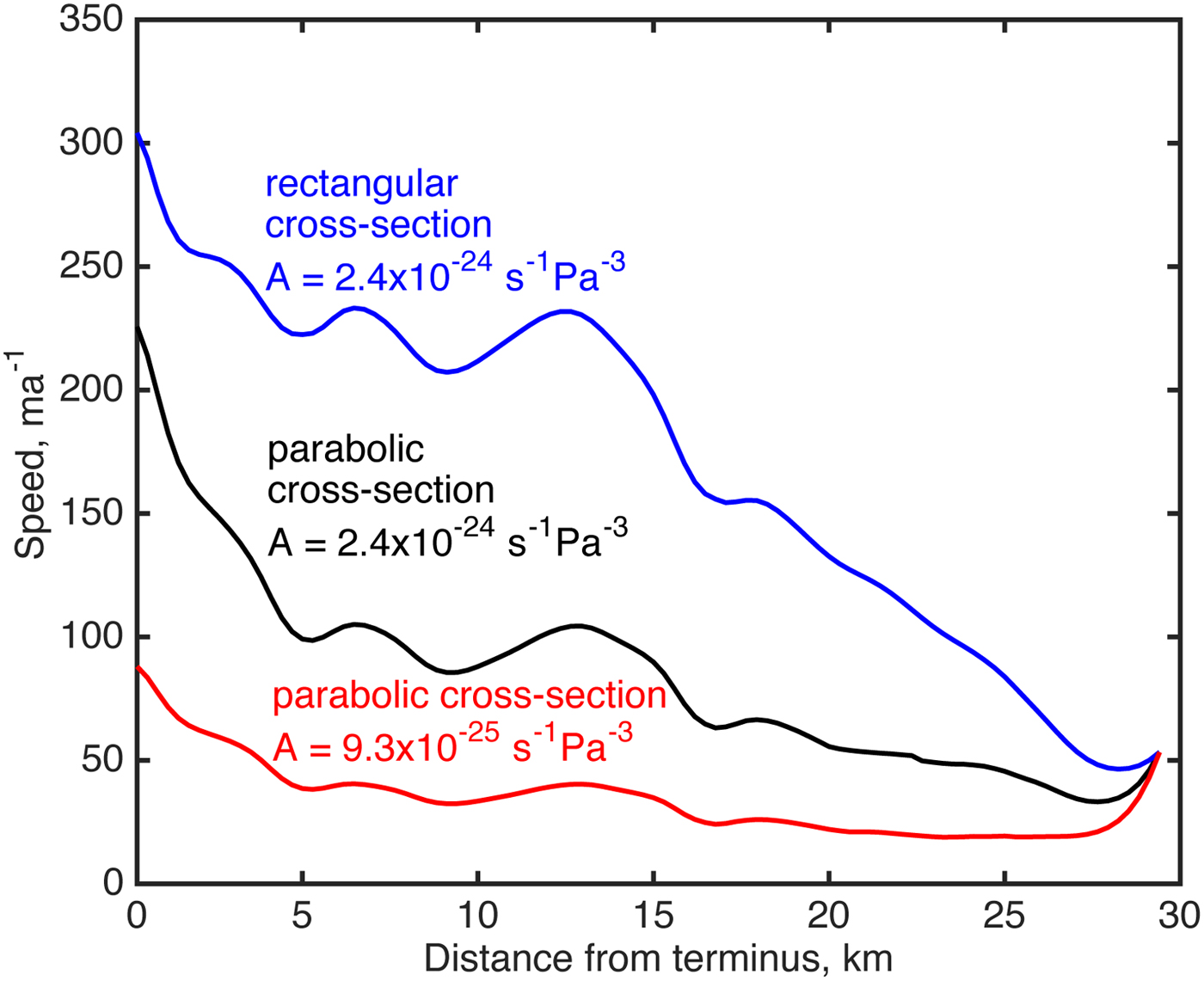
Including a representation of valley cross-sectional shape is important for producing winter baseline speeds that match the observations (Fig. 5). The importance of parameterizing glacier width for generating lateral drag was previously highlighted for an alpine glacier by Pimentel and others (Reference Pimentel, Flowers and Schoof2010). Here we highlight the key role of glacier width and shape for a large marine-terminating outlet glacier. Reduced width near the base of the glacier increases drag and decreases flowline speeds (Fig. 5). We find that both along-flow variations in width and reduced width with increasing depth (changing cross-sectional shape) are necessary to match observed flowline speeds in the absence of significant model recalibration. Although we do not explicitly explore the effect of channel shape on seasonal dynamics, we do expect it to play a role. For example, Enderlin and others (Reference Enderlin, Howatt and Vieli2013) have shown that the dynamic response of a marine-terminating outlet glacier to frontal perturbations is sensitive to glacier width variations.
Sea ice and tidal effects
Given our realistic simulated baseline flowspeeds, we now explore the effects of perturbations at the ice/ocean interface. We consider perturbations due to the effects of changing sea-ice (and or ice mélange) backstress and tidal forcing by changing the boundary conditions at the glacier terminus (Eqn (5)). Because our baseline flowspeeds were determined without buttressing, we examine only positive perturbations. Backstress applied at the ice/ocean interface reduces modelled terminus speeds below the baseline value (Fig 4a), with at least 150 kPa required to reach values similar to the lowest observed (from 8 February–3 March 2010). The application of such a backstress influences ice-surface speeds up to ~4 km from the terminus (Fig. 4a).
The maximum and minimum tidal elevations in 2008 were estimated using WebTide (a tidal prediction model developed by Fisheries and Oceans Canada) to be +1.68 m and –1.44 m, respectively. Here we compare the effects of a representative annual high tide (+1.50 m) with those of an annual low tide (–1.50 m) (Fig. 4b). Since tidal cycles continuously modulate sea level, contrasting the effects of an annual high tide and an annual low provides an upper limit on the influence of tidal forcing on glacier flowspeeds at the terminus. The modelled influence is small, compared with that of the backstress imposed to emulate sea ice (Fig. 4b).
Changes in backstress can produce the range of observed winter flowspeeds at the terminus derived from both remote sensing and in situ GPS data. The large observed intra-annual variability in flowspeed near the terminus and further up-glacier (Fig. 4c) cannot, however, be explained by variations in backstress alone.
Hydrologic controls
The hydrologic forcing differed significantly between the 2008 and 2009 melt seasons (Figs 6a and b). In 2008, two periods of run-off are separated by a near cessation of surface melt around day of year 206. In contrast, 2009 was characterized by a single dominant peak in run-off around day of year 208. Both the maximum and total run-off were greater in 2009 than 2008. However, surface-to-bed connections were established earlier in 2008 than 2009 (indicated by dots in Figs 6a and b).
Surface run-off, modelled evolution of the subglacial drainage system and modelled versus measured ice-surface speed for 2008 (left column) and 2009 (right column). (a) Estimated surface run-off time series from individual sub-catchments (lines), with the timing of surface-to-bed connections indicated (dots) for 2008. (b) As in (a) but for 2009. (c) Fraction of total simulated subglacial discharge routed through the conduit system as a function of time and distance from the glacier terminus for 2008. Warm colours indicate a conduit-dominated (efficient) drainage system, while cool colours indicate a sheet-dominated (inefficient) drainage system. Horizontal lines indicate the location and duration of meltwater input to the subglacial system, colour-coded by sub-catchment (see legend in (b)). (d) As in (c) but for 2009. (e) Daily modelled and measured ice-surface speeds at GPS locations in 2008. Modelled speeds with threshold drainage are shown as black lines and those with continuous drainage are shown as grey lines. Daily measured speeds, shown as blue lines, were computed as 24-hr running means from the GPS data. Station locations are given as distance from the glacier terminus in the upper right of each panel. Vertical red lines indicate the timing of surface-to-bed connections. (f) As in (e) but for 2009.

During times of high run-off, modelled subglacial drainage occurs preferentially in the conduit system (yellow colours in Figs 6c and d). The diminishing availability of surface water, combined with the absence of subglacial access points, in the uppermost reaches of the model domain inhibit conduit formation and result in sheet-dominated subglacial drainage (blue colours in Figs 6c and d). The dark blue vertical swaths in Figures 6c and d represent the rapid injection of water initially into the subglacial sheet, upon surface-to-bed connections (horizontal lines) in sub-catchments 2–5. No such perturbation occurs for sub-catchment 1, where a smaller amount of water is fed into the system through the upstream boundary condition. Similarly, this perturbation is absent from sub-catchment 5, as water is assumed to drain to the bed through multiple entry points.
The velocity time series from the uppermost GPS station is used to formulate the model boundary conditions, we therefore have five remaining time series (two from 2008, three from 2009) to compare with our model results (Figs 6e–i). We compare 24-hour running means computed from hourly GPS data with modelled daily flowline speeds from the gridcell that includes the GPS location. Broadly speaking, the baseline speeds match well (as seen also in Fig. 4a), and the timing and magnitude of the short-lived acceleration events share some common characteristics. However, the modelled peaks are sometimes more pronounced (e.g. Fig. 6h) and their timing not always coincident with observed peaks. The most marked discrepancy, however, is the absence in the model of prolonged periods of elevated flow rates that appear to be associated with run-off (especially close to the terminus, Figs 6e and f). The model response to melt is simply too abrupt and short-lived.
The model produces mean flowspeeds closer to the observed values at the GPS sites in 2008 than in 2009, as indicated by the smaller absolute error (column three in Table 3). For all five GPS time series, the mean modelled speeds during the melt season are lower than the mean measured values. The range in speeds, quantified as the difference between the 24-hour maximum and minimum values over the summer period (day of year 160–240), is best captured by the model close to the terminus (column four in Table 3). Two major velocity peaks are visible in the GPS data for 2008. The second of these events is much smaller in the model and is almost entirely absent near the terminus.
Statistics from the comparison of modelled and GPS-observed horizontal velocities (see Figs 6e–i), with two time series from 2008 and three from 2009
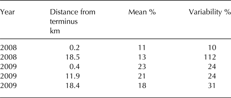
Mean is the percentage difference between the mean observed and mean modelled melt-season velocities (day of year 160–240) relative to observations. Variability is defined as the summer maximum minus the summer minimum and expressed as the percent difference between observed and modelled values relative to observations.
The rapid establishment of surface-to-bed connections (see Table 1) dominates the modelled melt-season flowspeeds in both 2008 and 2009 (Figs 6e–i). If surface meltwater is instead fed continuously into the modelled subglacial drainage system, the well-timed speed-up events are not captured. Figure 6f provides an example in which the observed peak in flowspeed around day of year 198 is only captured in the model when the observed drainage of a supraglacial lake in sub-catchment 5 is included.
In 2008, GPS-derived velocities decline to baseline values during the interval of near-zero run-off beginning around day of year 206. Velocities increase again to a second peak around day of year 215, near the second peak in run-off. In contrast, peak velocities lead peak runoff by at least 10 days in 2009. By the time run-off is at its maximum in 2009 (around day of year 208), velocities are already declining. The model results in Figures 6c, and d would support a standard explanation for the timing of run-off versus speed-up in the 2 years as related to the state of drainage-system development.
DISCUSSION
In this study we have considered the dynamic response of the tidewater-terminating Belcher Glacier to perturbations at the terminus and the basal boundary. We perturbed the terminus boundary condition using a backstress parameter to emulate the effect of changing sea ice and ice mélange conditions. The backstress that mélange exerts on a glacier front is uncertain, so various values have been used in the literature. For example, Krug and others (Reference Krug, Durand, Gagliardini and Weiss2015) investigated the impact of ice mélange on the advance and retreat cycles of glaciers with synthetic geometries using a range of backstress values up to 1 MPa. We explore values up to 300 kPa, but consider values <50 kPa to be realistic estimates of the constraining strength of the landfast seasonal sea ice and icebergs in front of Belcher Glacier. For comparison, Walter and others (Reference Walter2012) estimate a buttressing stress due to the presence of ice mélange at Store Gletscher, Greenland, to be ~30–60 kPa. We find that backstress alone cannot produce the magnitude or longitudinal extent of melt-season velocity variability observed at Belcher Glacier, leaving hydrologic forcing as the suspected driver. In a study of 16 glaciers in northwest Greenland, observed with and without the presence of ice mélange, Moon and others (Reference Moon, Joughin and Smith2015) also suggest that seasonal velocity changes are largely due to run-off forcing rather than changes in the extent and thickness of ice mélange. They note, in addition, that the magnitude of seasonal speed-up they calculate for these 16 glaciers is similar to that observed by other studies on land-terminating glaciers.
Herdes and others (Reference Herdes, Copland, Danielson and Sharp2012) showed that the break-up of landfast sea ice in front of Belcher Glacier for the years 1997 to 2008 consistently occurred in mid-July. The break-up was found to be correlated with the release of existing ice mélange and newly calved icebergs into the fjord. In 2008, break-up occurred on 16 July (day of year 196), well into the melt season (Figs 6a and b) and after the observed threshold drainage events (Table 1). Time-lapse photographs show that subglacial meltwater plumes, along with ocean currents and winds, push the weakened sea ice and icebergs away from the glacier front (Herdes and others, Reference Herdes, Copland, Danielson and Sharp2012). A decline in backstress due to weakening of the seasonal sea-ice matrix in the early part of the melt season (before threshold drainage) would be consistent with these observations and could contribute to the increase in near-terminus velocities. In spring we observe concentric folds and longitudinal fractures in the sea ice, emanating from the Belcher Glacier terminus, indicating that the sea ice and ice mélange resist the forward motion of the glacier in winter. The weakening of this resistive force may contribute to the steady velocity increase at the near-terminus GPS station that precedes the modelled speed-up (Figs 6e and f). The observed velocities appear to return to baseline values prior to the mid-to-late October formation of sea ice in front of Belcher Glacier (Herdes and others, Reference Herdes, Copland, Danielson and Sharp2012). Changes in backstress magnitude due to the sea ice could also have an influence on terminus velocities during the winter season or produce year-to-year differences.
Changes in terminus stress conditions at tidewater glaciers are also influenced by frontal submarine melting. Warm salty ocean water delivered by fjord circulation to the ice/ocean interface increases submarine melt that promotes undercutting and can trigger calving and accelerated ice flow (e.g. O'Leary and Christoffersen, Reference O'Leary and Christoffersen2013; Krug and others, Reference Krug, Durand, Gagliardini and Weiss2015). Several CTD profiles collected near the Belcher Glacier terminus and in deeper water toward the coastal shelf on 16 August 2011 reveal ocean water broadly characterized by three vertical layers: an upper warm layer, with temperatures between
 $0\! -\! 5 ^{\circ} {\rm C}$
in the top 30–50 m, an intermediate cool layer with temperatures below 0°C to a depth of ~280 m and a deep warm layer with temperatures ~
$0\! -\! 5 ^{\circ} {\rm C}$
in the top 30–50 m, an intermediate cool layer with temperatures below 0°C to a depth of ~280 m and a deep warm layer with temperatures ~
 $0 ^{\circ} {\rm C}$
. These profiles indicate that warmer deeper fjord water is not in contact with the ice front, and are significantly different from those in Greenland fjords where temperatures in the deep layers are >
$0 ^{\circ} {\rm C}$
. These profiles indicate that warmer deeper fjord water is not in contact with the ice front, and are significantly different from those in Greenland fjords where temperatures in the deep layers are >
 $0 ^{\circ} {\rm C}$
and can reach
$0 ^{\circ} {\rm C}$
and can reach
 $4 ^{\circ} {\rm C}$
(cf. Straneo and others, Reference Straneo2012). Unlike several Greenland outlet glaciers, Belcher Glacier does not exhibit straightforward evidence of submarine melt-induced thinning from warm ocean waters at depth. Submarine melting is therefore not considered a significant contributor to reduced buttressing and backstress at the Belcher Glacier terminus.
$4 ^{\circ} {\rm C}$
(cf. Straneo and others, Reference Straneo2012). Unlike several Greenland outlet glaciers, Belcher Glacier does not exhibit straightforward evidence of submarine melt-induced thinning from warm ocean waters at depth. Submarine melting is therefore not considered a significant contributor to reduced buttressing and backstress at the Belcher Glacier terminus.
Recent studies from Greenland have highlighted the prominent role of subglacial discharge in contributing to submarine melt (e.g. Beaird and others, Reference Beaird, Straneo and Jenkins2015; Fried and others, Reference Fried2015; Carroll and others, Reference Carroll2016). Subglacial plumes have been proposed to drive warm saline water toward glacier termini during the melt season and generate buoyancy-driven melt, including in relatively cold and shallow Greenland fjords similar to those of Belcher Glacier (Carroll and others, Reference Carroll2016). A turbid meltwater plume is visible in the time-lapse photographs from Belcher Glacier terminus and was persistent from year to year close to the southern edge of the terminus. Localized lowering of the ice surface and a concentration of iceberg calving at this location suggest the occurrence of submarine melting due to subglacial discharge. Additional subglacial outlets may exist that do not produce observable plumes but still contribute to submarine melt, as found by Fried and others (Reference Fried2015) at a tidewater glacier in central West Greenland. An analysis of water types from another proglacial fjord in Greenland indicates submarine-melt-driven convection and convection-driven melt from surface run-off at the ice/ocean interface suggesting multiple melt processes may be important (Beaird and others, Reference Beaird, Straneo and Jenkins2015). Such ice/ocean boundary processes may promote calving and frontal ice loss at Belcher Glacier. The resultant retreat of the terminus, and associated reduction in buttressing, may cause accelerated ice flow. Although interannual and seasonal changes to the Belcher Glacier terminus position are small enough to be within a single model gridcell, the changing stress conditions likely have some impact on near-terminus flow velocities.
In the hydrologically-driven melt-season simulations, we find that threshold drainage events generate strong initial speed-up events in the first half of the melt season (similar to Joughin and others, Reference Joughin2013). Significant early-season speed-up events are not captured by the model when we assume surface-to-bed connections to be open from the onset of the melt season (Figs 6e–i). Meltwater that impinges on the inefficient drainage system decreases effective pressure and enhances glacier slip. This influx of meltwater then leads to conduit development in the model and a more efficient drainage system, thereby increasing effective pressures and reducing glacier slip. The greatest changes in modelled speed occur during sharp increases in meltwater input (e.g. day 183 (2008) and day 193 (2009)) rather than during periods of peak run-off (which occur much later in the melt season, see Fig 6a and b), consistent with Schoof (Reference Schoof2010). For example, GPS-derived ice-surface velocities decrease from around day 206 in 2009, while run-off is still high (Fig. 6). This observation suggests that an efficient drainage system has been established, and is in line with the model results showing dominance of conduit discharge at this time (Fig. 6d).
In the first half of the melt season, after the initial surface-to-bed connections have been established, a channelized drainage system develops in the model and brings to an end the velocity increase, whereas the observations show that higher velocities persist for several days. This model–data mismatch could be the result of overly vigorous channel development in the model, or the presence of episodic drainage events and/or additional drainage locations that are not adequately captured in the observationally-derived model inputs. Configuring the model to converge in the presence of sudden large influxes of meltwater requires parameter choices that reduce model sensitivity, and therefore reduce the magnitude of the modelled velocity response to drainage events later in the meltseason. Limitations to model–data comparison also arise from the spatial and temporal differences in modelled versus measured flowspeeds. The measured speeds represent point-scale values based on hourly GPS data, while the modelled speeds represent gridcell-averaged flowline values obtained with daily (rather than hourly) forcing.
CONCLUSION
Using a hydrologically-coupled higher-order ice flow model, we have examined the dynamics of Belcher Glacier in response to variations in frontal buttressing and melt-season hydrology. A realistic representation of valley width and cross-sectional shape, along with a novel approach to accounting for tributary fluxes in a flowband model, allows us to simulate the general spatial structure of observed winter flow speeds. Buttressing at the ice/ocean interface was explored through perturbations intended to represent tidal cycles and changes in sea-ice and ice-mélange conditions. Tidal effects are found to have minimal influence on the glacier flow speed at the terminus. Reductions in flow speed commensurate with observations along the lowermost 4 km of the glacier can be achieved with a prescribed backstress of 150 kPa. This result suggests that variations in pre- and early melt season terminus velocities and year-to-year differences in winter terminus velocities could be influenced by seasonal and interannual sea-ice and ice-mélange dynamics. However, the large seasonal variability in flow speeds observed at Belcher Glacier (Fig. 4c), both near the terminus and further up-glacier, can only be emulated with hydrologic forcing. It is a shortcoming of our modelling study that some processes at the calving front are left unresolved. For example, we do not allow for changes to frontal geometry, do not include a process-based calving law and do not account for submarine melt due to subglacial discharge, all of which likely have some influence on near-terminus flow speeds. We used a distributed surface energy-balance and sub-surface snow model to generate time series of run-off for five sub-catchments of Belcher Glacier. Time-lapse photography and remote sensing are used to locate sub-catchment drainage points and to ascertain the timing of major supraglacial lake drainage events.
We find that an efficient drainage system develops in the model following threshold drainage events of meltwater from the surface. This system persists through the melt season downstream of the meltwater input locations, provided a sufficient supply of water. Modelled flow speeds resemble GPS-derived flow speeds in the timing of glacier acceleration following threshold drainage events, but fail to capture the prolonged periods of enhanced flow speed that appear closely associated with run-off (Fig. 6). Shortcomings in our drainage scenarios and process representation in the numerical model, as well as poorly constrained model parameters, may explain why modelled speed-up events are short-lived relative to events in the GPS records. The 2008 and 2009 run-off hydrographs are very different, with the 2009 season exhibiting one distinct peak rather than two, and having a greater maximum and total run-off than 2008. These features are evident in the behaviour of the modelled subglacial drainage system, with efficient drainage being sustained for a longer period and reaching further up-glacier in 2009 than 2008.
Overall, we find that hydrologic forcing plays a greater role than frontal buttressing in the intra-annual dynamics of Belcher Glacier assessed through GPS and remote sensing observations from 2008 and 2009. Knowledge of meltwater input locations and the timing of surface-to-bed connection events are important for understanding and modelling the flow patterns at this tidewater outlet glacier. In addition to the hydrological and ice/ocean processes explored here, future work should examine the role of submarine melt processes and changes in terminus position as additional drivers of Belcher Glacier dynamics.
ACKNOWLEDGEMENTS
This study was funded by the Natural Sciences and Engineering Research Council (NSERC) of Canada, through the International Polar Year Special Research Opportunity fund. Support for fieldwork on Belcher Glacier was provided by Polar Continental Shelf Program and the Canada Foundation for Innovation. We thank the Nunavut Research Institute and the communities of Grise Fjord and Resolute Bay for permission to conduct fieldwork on Belcher Glacier. We are grateful to James Davis, Alex Gardner, Emilie Herdes, Hannah Milne and Tyler Sylvestre for help in the field and to the anonymous reviewers, the Scientific Editor Fiamma Straneo and the Chief Editor Helen Amanda Fricker for their careful and constructive comments, which resulted in a substantially improved manuscript.


 Open access