


1. Introduction
Shock waves occurring during cavitating bubble collapse have always fascinated scientists as one of the most destructive forces in nature. Cavitation is the phenomenon where individual bubbles or bubble clouds vigorously oscillate and violently collapse due to instantaneous pressure fluctuations in a liquid. As they implode, cavitation bubbles produce high-speed liquid jets (typically above 100 m s−1) (Tzanakis et al. Reference Tan, Lee, Khong, Connolley, Fezzaa and Mi2014) and omnidirectional shock waves with local pressure spikes in the range of gigapascals (Pishchalnikov et al. Reference Petkovšek, Hočevar and Dular2019). Accurate determination of the shock wave characteristics is essential in controlling the effectiveness of the external processing conditions on various physical, chemical and biological systems. Shock waves are of importance due to their extreme dynamics, and underpin many of the applications that utilize acoustic cavitation, notably melt treatment (Meyers, Gupta & Murr Reference Mettin1981; Eskin & Eskin Reference Eskin and Eskin2014; Tan et al. Reference Suslick2015; Eskin & Mi Reference Eskin and Mi2018; Eskin et al. Reference Eskin, Tzanakis, Wang, Lebon, Subroto, Pericleous and Mi2019), sonochemistry (Suslick Reference Song, Johansen and Prentice1990), lithotripsy (Church Reference Church1989; Zhong, Chuong & Preminger Reference Yusuf, Symes and Prentice1993Reference Zhong, Chuong and Preminger; Vogel Reference Tzanakis, Lebon, Eskin and Pericleous1997; Bailey et al. Reference Bailey, Pishchalnikov, Sapozhnikov, Cleveland, McAteer, Miller, Pishchalnikova, Connors, Crum and Evan2005; Cleveland & McAteer Reference Cleveland and McAteer2007; Kobayashi, Kodama & Takahira Reference Johnston, Tapia-Siles, Gerold, Postema, Cochran, Cuschieri and Prentice2011; Pishchalnikov et al. Reference Petkovšek, Hočevar and Dular2019), ocular surgery (Vogel et al. Reference Vogel, Busch and Parlitz1986), food processing (Long Reference Lebon, Tzanakis, Pericleous and Eskin2001) and pharmaceutics (Dalecki Reference Dalecki2004; Menezes et al. Reference Long2008), to name but a few. Furthermore, it has recently been discussed, as part of the present studies, that shock wave emission is the governing mechanism for intermetallics fragmentation (Priyadarshi et al. Reference Pishchalnikov, Behnke-Parks, Schmidmayer, Maeda, Colonius, Kenny and Laser2020) as well as for graphite exfoliation (Morton et al. Reference Morris, Hurrell, Shaw, Zhang and Beard2021). However, the key properties of cavitation-driven shock waves and the underlying shock wave mechanisms are not well understood and therefore remain a topic of great interest.
Acoustic pressure measurements can be essential for quantifying and understanding shock wave propagation. There have been several works dealing with experimental pressure measurements and numerical predictions in the presence of a shock wave (Doukas et al. Reference Doukas, Zweig, Frisoli, Birngruber and Deutsch1991; Vogel, Busch & Parlitz Reference Vogel1996; Pecha & Gompf Reference Neppiras2000; Možina & Močnik Reference Moussatov, Granger and Dubus2005; Gregorcic & Mozina Reference Gregorcic and Mozina2007; Brujan, Ikeda & Matsumoto Reference Brujan, Ikeda and Matsumoto2008; Holzfuss Reference Holzfuss2010; Brujan, Ikeda & Matsumoto Reference Brujan, Ikeda and Matsumoto2012). However, to the best of our knowledge, a full spectrum analysis (especially in the megahertz range) and pressure mapping of the acoustic cavitation-induced shock waves associated with the high-intensity ultrasonic energy generated at low driving frequencies, i.e. 17–30 kHz (so called power ultrasound), have not been performed yet, whereas the application of power ultrasound is widespread and essential for many applications. The majority of reported studies on shock waves have been focused on medical applications and were related to transducers with significantly higher driving frequencies, e.g. 692 kHz (Song, Johansen & Prentice Reference Son, Lim, Khim and Ashokkumar2016), 254 kHz (Johnston et al. Reference Johansen, Song and Prentice2014; Johansen, Song & Prentice Reference Johansen, Song, Johnston and Prentice2018) and 1.1 MHz (Brujan, Ikeda & Matsumoto Reference Brujan, Ikeda and Matsumoto2012), with results showing that shock waves are responsible for the rise of subharmonic peaks and the noise floor. Furthermore, previous studies with low driving frequencies (Laborde et al. Reference Kobayashi, Kodama and Takahira1998; Moholkar, Sable & Pandit Reference Meyers, Gupta and Murr2000; Son et al. Reference Settles2012) were carried out for low acoustic power intensities (0.3–3 W cm−2) with pressure amplitudes being mostly scrutinized for the harmonics and subharmonics to the driving frequency in the kilohertz range. In contrast, this work employs a system combining high power densities (90–460 W cm−2) with a low acoustic driving frequency (24 kHz), known to produce a broad spectrum of pressure peaks associated with shock waves arising from inertial cavitation events, resonating nodes due to the container dimensions and harmonics from stably oscillating bubbles.
Highly sensitive fibre-optic hydrophones (FOHs) that are calibrated for a broad range of megahertz frequencies (associated with shock wave emissions) have been deployed (Morris et al. Reference Möller, Degen and Dual2009), since the strong adhesion between their optical fibre and the liquid enables the sensor to seize the tensile phase of the shock wave, avoiding the possibility of cavitation taking place at the surface of the probe (Cleveland & McAteer Reference Cleveland and McAteer2007; Morris et al. Reference Möller, Degen and Dual2009) to ensure that no additional noise or signals are captured. This allowed the frequency spectrum of shock waves in the range above 1 MHz produced by a low-frequency transducer (24 kHz) to be resolved via detailed pressure measurements. We present a comprehensive experimental study to understand in detail the shock wave mechanisms and dynamic features in a sonicated environment with high-precision measurement tools. We intentionally used a broadly calibrated FOH at high frequencies to capture all the detailed spectral features in the megahertz range associated with transient cavitation and shock wave emissions. Pressure measurements were supplemented with visualization techniques. A spatial pressure map was constructed by collating individual pressure measurements taken in the vicinity of the ultrasonic source (and up to 10 mm distant) to provide a better understanding of the physics of acoustic cavitation and associated emission of shock waves produced by collapsing bubble structures.
2. Experimental set-up
A schematic of our experimental set-up is shown in figure 1. An FOH (Precision Acoustics Ltd) was fixed on a plastic holder and mounted at the bottom of a glass tank with internal dimensions 300 mm × 75 mm × 100 mm. The probe has an outer diameter of 125 μm and the optically illuminated core (which defines the active element) has a diameter of 10 μm. The very small active element ensures that the FOH has a very broad directional response below 15 MHz (Morris et al. Reference Möller, Degen and Dual2009). All probe type hydrophones, including the FOH, have a peak in their directional response when their active element is pointed at the source of the ultrasonic signal. For the measurements reported here, it is not possible to know, a priori, the precise location of a bubble that is undergoing cavitation. Therefore, the hydrophone should be, as far as is possible, equally responsive to acoustic signals, regardless of their angle of incidence upon the hydrophone. The FOH was calibrated over the range of 1–30 MHz at 1 MHz increments (see figure S1 in the supplementary material available at https://doi.org/10.1017/jfm.2021.186). Sonication was applied by a 24 kHz transducer (UP200S, Hielscher Ultrasonics GmbH) to the deionized (DI) water inside the tank. The water level was 80 mm and the diameter of the cylindrical Ti sonotrode tip was 3 mm. Across the tank, 136 locations were chosen for the measurement of acoustic pressure emissions. All experiments for each position were performed for three different input transducer powers, 20 %, 60 % and 100 %, corresponding to peak-to-peak displacement amplitudes of 42, 126 and 210 μm and nominal intensities of 92, 276 and 460 W cm−2, respectively. These power intensities are much larger than in similar studies with low driving frequencies (3.2 W cm−2 in Laborde et al. (Reference Kobayashi, Kodama and Takahira1998), 0.3–0.95 W cm−2 in Son et al. (Reference Settles2012) and 0.53 W cm−2 in Moholkar, Sable & Pandit (Reference Meyers, Gupta and Murr2000)). The inset plot in figure 1 shows where the probe was placed: at  $- 10 \le x \le 10 \ \textrm{mm}$ and $1 \le y \le 10\;\textrm{mm}$, with the centre of the sonotrode tip taken as the origin. This gave us an extensive symmetric map of the pressure distribution around the sonication source.
Experimental set-up for pressure measurement by the FOH. A small sonotrode is immersed in the glass tank filled with DI water. The signals are captured by a PicoScope, setting the sampling rate (resolution). A high-speed camera (HPV X2, Shimadzu) captures the shock wave propagation. And 10 ns laser pulses (640 nm) by CAVILUX Smart UHS provides the required illumination.

To ensure the safe functionality of the FOH sensor, each experiment lasted for 5–10 s (until steady-state conditions were achieved) and the closest distance of the hydrophone tip from the source was chosen to be 1 mm. The temperature was kept constant at 25 °C during the experiments. Furthermore, we used a high-speed camera (HPV X2, Shimadzu, Japan) to capture the shock wave emission. High-speed recordings were carried out at frame rates of up to one million frames per second, with a resolution of 400 × 250 pixels and 200 ns exposure time. The illumination was delivered by 10 ns laser pulses (640 nm) from a CAVILUX Smart UHS system (Cavitar Ltd) to create an effective temporal resolution of emitted shock waves. The detailed experimental set-up for high-speed recordings of shock waves facilitates shadowgraphic imaging such that pressure transients are directly imaged via refractive index variations imposed as the shock wave propagates and is described elsewhere (Johansen 2018; Yusuf, Symes & Prentice Reference Yasui, Iida, Tuziuti, Kozuka and Towata2021). The FOH was manually fixed on the tank (as shown in figure 1), but, for each experiment, the tank was traversed using translational stages to place the FOH at the desired position measured precisely by high-speed camera.
Acoustic pressure emissions were captured using a digital oscilloscope (PicoScope-3204D, Pico Technology) through the output of the FOH system. The electronic connection of the sensor is schematically represented in figure 1. The PicoScope captured and recorded real-time acoustic data for 60 random waveforms (to ensure repeatability and to average out the effect of the random nature of cavitation) under steady-state conditions. The sampling rate was  $500 \times {10^6}\;\textrm{samples}\;{\textrm{s}^{ - 1}}$. The entire analysis of the experimental data was carried out via an in-house MATLAB code based on the deconvolution process as described previously (Hurrell Reference Hurrell2004; Hurrell & Rajagopal Reference Hurrell and Rajagopal2016; Johansen et al. Reference Johansen2017; Lebon et al. Reference Laborde, Bouyer, Caltagirone and Gérard2018) and in Appendix D in IEC (Reference Dalecki2013) to correctly apply the sensitivity of the FOH (see figures S1 and S2 in the supplementary material). The MATLAB code ultimately calculates the desired pressure magnitudes in the time domain from the original voltage data acquired by the PicoScope. Background noise (~10 mV) was recorded and subtracted from the raw signals, and bandpass filters (in the calibration range 1–30 MHz) were applied to avoid the contribution of the non-calibrated range of FOH. Furthermore, from the high-speed recordings, we utilized image-processing techniques to measure the wavelength of the shock wave disturbance and consequently to infer its frequency.
3. Results and discussion
Figure 2 shows a sample of pressure in the frequency domain, clearly demonstrating a distinct peak in the high-frequency range of 3–4 MHz. The inset in figure 2 shows the magnified area near the peak frequency, which shows that the peak occurs within a frequency bandwidth of 3.27–3.43 MHz. This high-frequency peak was observed for all the experiments irrespective of position or input power. See supplementary movie SV1 for the entire P–f plots (with their prominent peak) for all 136 positions and input powers of 20 %, 60 % and 100 % along with their corresponding probe position marked around the sonotrode. Our hypothesis is that this distinct peak in the pressure spectrum is the result of cavitation activity and shock wave emissions due to bubble implosions. To investigate whether acoustic cavitation is responsible for this, we performed a number of additional experiments for different conditions to eliminate other possible sources that can potentially contribute to that frequency peak, such as interference from acoustic resonance, effects of transducer, different probe, sonotrode size, presence of glass walls and possible electromagnetic interference (see figures S4–S8 and table S1 in the supplementary material).
Pressure versus frequency measured by the FOH. The inset magnifies the plot near the distinct peak frequency. For this experiment, the probe was at  $x = 0$ and $y = 1\;\textrm{mm}$ and the input power was 60 %. The pressure was averaged over 60 waveforms. The pressure at the peak frequency is $0.479 \pm 0.06\;\textrm{kPa}$.

When we used a different transducer and sonotrode (figures S4 and S5) and a different probe (figure S6), we still observed the peak. Placing the probe and sonotrode far from each other, putting a glass wall between them (figure S7) and covering the probe with an acoustically reflective material (to see if electromagnetic interference can contribute to the peak; see figure S8) either weakened or suppressed the peak. Therefore, these additional experiments strengthen our hypothesis that the shock wave propagation due to bubble collapses might be the plausible cause of the observed peak at 3.27–3.43 MHz frequency. It should be noted that the broadband nature of the shock wave distributes its power (not necessarily equally) over almost all frequencies, across a flat-wise spectrum (see figure S9). Therefore, this peak contains a portion of the power content of the shock wave, while the rest of its power is distributed over all other frequencies.
The majority of the previous studies on shock wave measurements and visualizations were performed for a single bubble collapse and the consequent analysis of a single or a few shock waves showed that, apart from the energy that is spread over a very large frequency range, a prominent though obscured peak can also be observed, indicating that even those individual shock waves can still lead to a peak in the frequency domain (Cleveland & McAteer Reference Cleveland and McAteer2007; Johansen et al. Reference Johansen2017). However, in our case, we are facing multiple shock waves, due to the continuous formation and collapse of cavitation-induced bubbles. Thus, an ensemble of imploding bubbles and the consequent piling up of numerous shock waves may lead to this prominent peak that is sensed by FOH. However, the energy of these bubble collapses is not strong enough for the probe to pick up the subsequent harmonics.
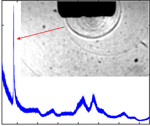
To further examine the measured shock wave frequency, using the Schlieren (Settles Reference Priyadarshi, Khavari, Subroto, Conte, Prentice, Pericleous, Eskin, Durodola and Tzanakis2012; Möller, Degen & Dual Reference Moholkar, Sable and Pandit2013) method, we analysed the high-speed images of shock wave emission to extract the wavelength of the disturbance and consequently the frequency. Figure 3 shows a snapshot of a propagation of the shock wave along with the distribution of optical intensity across the shock wave (distance d from point a towards b). The shock wave and the sonication source (sonotrode) are specified in the figure. The intensity profile shows a full cycle of the wave from which the wavelength  $(\lambda )$ and consequently the frequency of the emission can be measured. The optical intensity is proportional to the second derivative of the index of rarefaction (Evans Reference Evans1990; Settles Reference Priyadarshi, Khavari, Subroto, Conte, Prentice, Pericleous, Eskin, Durodola and Tzanakis2012) as well as that of pressure (Chamanzar et al. Reference Chamanzar, Scopelliti, Bloch, Do, Huh, Seo, Iafrati, Sohal, Alam and Maharbiz2019). Thus, the change in the optical intensity (diffraction of light) is due to the change in acoustic pressure as the pressure waves propagate through the liquid bulk. Therefore, the wave front can be considered as the compression phase, and the tail as the rarefaction phase, typical of a shock wave profile (Cleveland & McAteer Reference Cleveland and McAteer2007). As a result, measuring the speed of sound and the wavelength from the high-speed recordings can give us the frequency of the wave propagation.
A snapshot of shock wave propagation (a) along with the intensity profile (b) across the shock wave. The intensity profile shows how the wavelength  $(\lambda )$ and consequently the frequency can be calculated. Arrows show the sonotrode and shock wave. The red dashed rectangle magnifies the shock wave for better visualization. Scale bar is 2 mm.

After monitoring the propagation of multiple shock fronts in our entire experiments, the mean speed of the shock wave emission (speed of sound) was measured to be  $1464 \pm 5\;\textrm{m}\;{\textrm{s}^{ - 1}}$ and pixel size was $39.02 \pm 4\;{\rm \mu} \mathrm{m}$. For the case in figure 3, this frequency was found to be 4.2 MHz. We measured this frequency for numerous shock waves (around 300) for six different experiments with different input powers (20 %, 40 % and 60 %) and found the average frequency to be $4.78 \pm 0.3\;\textrm{MHz}$ (the corresponding average wavelength was $315 \pm 20\;{\rm \mu} \mathrm{m}$). This value is reasonably close to the calculated value from the deconvolution process, i.e. 3.27–3.43 MHz (see figure S10 in the supplementary material for the measured frequency for different cases of different experiments and their corresponding mean value for each experiment). A detailed discussion of this discrepancy is to be found in the supplementary material (see figure S11).
The formation of shock waves has a profound effect on the overall pressure distribution in the liquid. We are going to demonstrate this by measuring the pressure profiles and then correlating these observations to the shock waves. The final output of the deconvolution process is the desired pressure profile in the time domain used to measure the maximum and root-mean-square (r.m.s.) pressures ( ${P_{max}}$ and ${P_{rms}}$), averaged over 60 waveforms for each experiment. Figures 4 and 5 show the contour plots of ${P_{max}}$ and ${P_{rms}}$ distribution versus horizontal and vertical position surrounding the sonotrode for three different transducer powers: (a) 20 %, (b) 60 % and (c) 100 % (see figures S12 and S13 in the supplementary material for the contour plots of ${P_{max}}$ and ${P_{rms}}$ versus input power). It is evident from figure 4 that
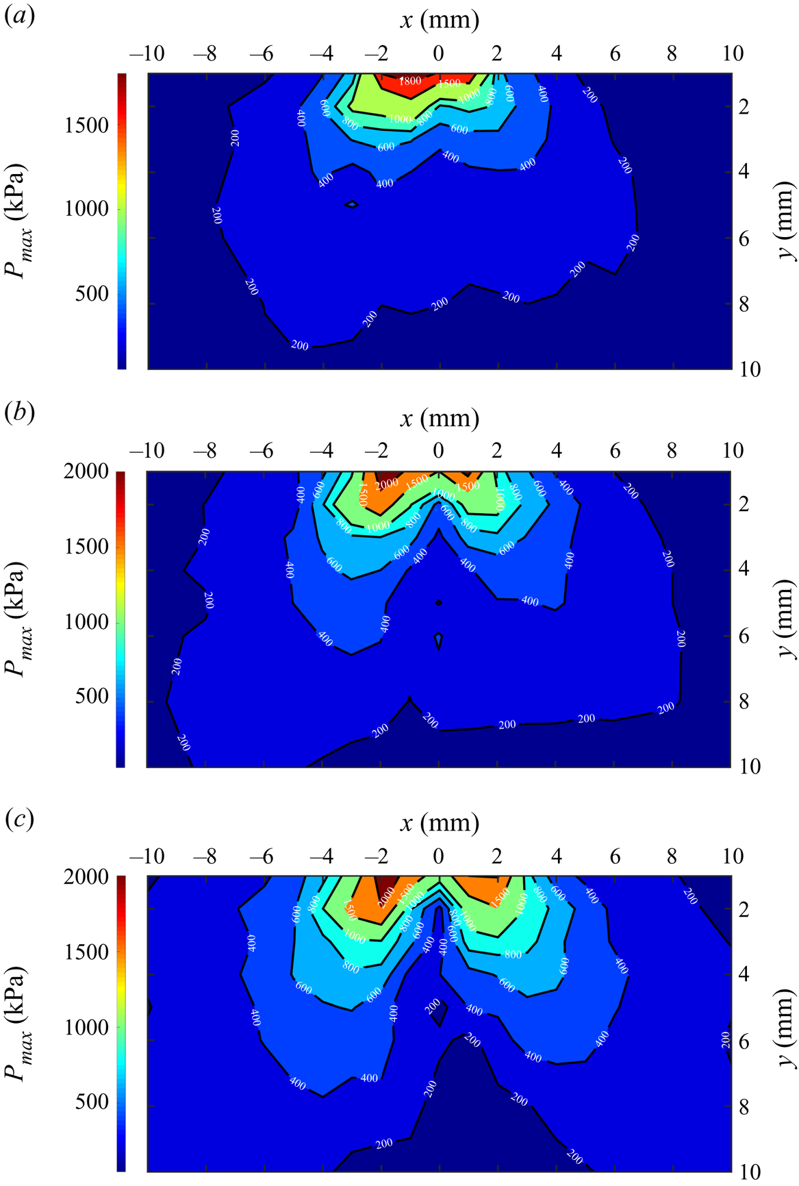
  ${P_{max}}$ is largest just under and in the closest proximity to the sonotrode, but, as the FOH probe moves away from the source, ${P_{max}}$ drops significantly. A similar behaviour is observed for r.m.s. pressure near to and far from the source (figure 5). In fact, our measurements show that within the 10 mm distance in the map of observation, ${P_{max}}$ drops by 97–98 % for all input powers. The corresponding drop for ${P_{rms}}$ was 75–78 %. Furthermore, it is clear from these plots that considerably larger peak pressure magnitudes are obtained only in the regions very close to the sonotrode, i.e. in areas where bubble concentration is likely to be the highest, indicating a strong nonlinear vibration mode of bubbles (transient cavitation) (Hamilton & Blackstock Reference Hamilton and Blackstock1998; Naugolnykh & Ostrovsky Reference Možina and Močnik1998; Campos-Pozuelo et al. Reference Campos-Pozuelo, Granger, Vanhille, Moussatov and Dubus2005). Additionally, the contour plots show high-pressure regions near the source as well as the non-symmetrical shape of the cavitation zone; the latter becomes less symmetrical with increase in power (the oscillation amplitude of the sonotrode). As the cavitation intensity near the sonotrode increases (increase of input power), a significant drop in the measured acoustic pressure close to the centre of the radiating surface can be observed. Note how the maximum pressure $({P_{max}})$ drops by almost one order of magnitude over a distance less than 10 mm away from the source for all input powers.
Contour plots of  ${P_{max}}$ around the sonotrode for three different transducer powers: (a) 20 %, (b) 60 % and (c) 100 %. The sonotrode is at (0, 0).
Contour plots of  ${P_{rms}}$ around the sonotrode for three different transducer powers: (a) 20 %, (b) 60 % and (c) 100 %. The sonotrode is at (0, 0).

This decrease in the peak pressure amplitude, especially for the case of 60 % and 100 % power, can be attributed to the cavitation shielding effect caused by the bubble cloud formation (Moussatov, Granger & Dubus Reference Morton, Khavari, Qin, Maciejewska, Grobert, Eskin, Mi, Porfyrakis, Prentice and Tzanakis2003) at the horn surface that restricts the propagation of the driving acoustic field and corresponding cavitation emissions into the medium (Lebon et al. Reference Laborde, Bouyer, Caltagirone and Gérard2018). This is in good agreement with previous observations, where the conical shape structure is believed to absorb the acoustic emissions, weakening the cavitation impact (Moussatov, Granger & Dubus Reference Morton, Khavari, Qin, Maciejewska, Grobert, Eskin, Mi, Porfyrakis, Prentice and Tzanakis2003; Yasui et al. Reference Vogel, Hentschel, Holzfuss and Lauterborn2008; Tzanakis et al. Reference Tzanakis, Eskin, Georgoulas and Fytanidis2016, Reference Tzanakis, Hodnett, Lebon, Dezhkunov and Eskin2017; Lebon et al. Reference Laborde, Bouyer, Caltagirone and Gérard2018). As the cavitation cloud intensifies with the input power, the shielding becomes stronger, which leads to weakening the pressure field at some short distance (Mettin Reference Menezes, Takayama, Gojani and Hosseini2005). Another possibility for a weakening pressure field and decreasing cavitation intensity is the absence of periodic bubble collapses as observed in Yusuf, Symes & Prentice (Reference Yasui, Iida, Tuziuti, Kozuka and Towata2021). In this recent work, an erratic behaviour of cavitation intensity for different input powers associated with shock wave emissions was shown. It was attributed to the local minima in the acoustic data observed with increasing sonotrode intensity (increased input power) caused by extended periods of non-collapsing deflations and thus the absence of shock wave generation. This is in line with previous observations (Tzanakis et al. Reference Tzanakis, Eskin, Georgoulas and Fytanidis2016), where a similar behaviour was noticed.
On the other hand, the study by Son et al. (Reference Settles2012) showed that the increase in input power resulted in an increase in the acoustic emissions only at derivative frequencies such as harmonics and subharmonics. However, it should be noted that this might also be related to the shock wave propagation and the spatial distribution of the cavitation energy at those frequencies, as it is known that subharmonics arise from transient cavitation events and the associated shock waves, while their interaction with bubbles in their pathway (as bubbles absorb part of the shock wave energy) triggers more stable cavitation events that are superimposed onto the existing harmonic or superharmonic spectral features (Neppiras Reference Naugolnykh and Ostrovsky1968; Petkovšek, Hočevar & Dular Reference Pecha and Gompf2020) of the fundamental frequency. Hence, the magnitude of cavitation intensity is inextricably linked to the shock waves and their propagation towards the bulk liquid.
It is evident that, at an input power of 20 % (figures 4a and 5a), where bubbly structures are rather weak and disjointed (Tzanakis et al. Reference Tzanakis, Hodnett, Lebon, Dezhkunov and Eskin2017), a rather uniform pressure field is formed below the sonotrode with a lower shielding effect as compared to that of the 60 % (figures 4b and 5b) and 100 % (figures 4c and 5c) power regimes. Furthermore, as can be seen more clearly in figure 5,  ${P_{rms}}$ (being statistically more robust than ${P_{max}}$) does not exhibit a symmetric pressure distribution (as expected), since the cavitation zone is ‘dancing’ continuously and propagating at various directions. This is a characteristic feature of the stochastic cavitation phenomenon. As seen in figure 5, in our case the cavitation zone mostly points towards the left $( - x)$ regions (possible structural tilt of the sonotrode tip) and consequently gives rise to more bubble collapses there, as the bubbly clouds are thrust to the left; therefore, the pressure is expected to be higher in those regions, and this is well captured by the FOH probe.
Furthermore, the presence of bubble clouds indicates the propagation of the shock waves and, most importantly, where the shock waves are mostly absorbed. At low input power (see supplementary movie SV2, power 20 %), the shock wave, while passing through the right side of the sonotrode, interacts with tiny cavitation nuclei and generates bubbles (i.e. the nuclei grow to form bubbles), which means that the shock wave should be less strong at this side than at the left side, where the shock wave propagates undisturbed (Petkovšek, Hočevar & Dular Reference Pecha and Gompf2020). This agrees well with the pressure contours in figure 5. On the other hand, at higher power (see supplementary movie SV3, power 60 %), the majority of the bubbles are observed in the central region just below the source (sonotrode axis), leading to energy absorption in that zone. Therefore, the shock waves are weakened around the axis of symmetry and are stronger at the edges, again in agreement with the pressure contours in figure 4.
Figure 6 shows the maximum pressure  ${P_{max}}$ of our entire sets of experiments for all horizontal (left and right) and vertical positions for all three transducer powers (20 %, 60 % and 100 %), versus the radial position $(r)$ measured from the source $(r = \sqrt {{x^2} + {y^2}} )$. Interestingly, the data fit well with the $1/r$ scale, as was previously suggested based on theoretical grounds (Vogel, Busch & Parlitz Reference Vogel1996) or numerical calculations of shock wave velocity (Holzfuss, Rüggeberg & Billo Reference Holzfuss, Rüggeberg and Billo1998; Holzfuss Reference Holzfuss2010). We can now verify this scale by direct experimental pressure measurements. According to figure 6, the pressure drop away from the sonotrode may be explained by the fact that the shock wave is briefly supersonic upon formation and loses its energy quickly afterwards (Vogel, Busch & Parlitz Reference Vogel1996; Johansen 2018). The individual fitting equations for each input power are ${P_{20\,\%}} = 2.29/{r^{ - 1.1}}$, ${P_{60\,\%}} = 2.31/{r^{ - 0.99}}$ and ${P_{100\,\%}} = 2.22/{r^{ - 0.85}}$. The reason for the multiple pressure magnitudes for the same position in figure 6 is that several different positions with the same r value have different x and y coordinates.
Plot of  ${P_{max}}$ versus r for the entire experimental matrix (all horizontal and vertical positions and input powers).

This is expected, as the strength of the shock wave pressure across the spatial positions hugely depends on the speed of the propagating shock fronts. It has been reported that the speed of a shock wave within 100 μm from the acoustic source is close to 2500 m s−1 and becomes equal to the speed of sound beyond the source (Brujan, Ikeda & Matsumoto Reference Brujan, Ikeda and Matsumoto2008). Also, previous studies confirm the significant dissipation of shock wave mechanical energy within the first 10 mm of its propagation (Vogel, Busch & Parlitz Reference Vogel1996). Note that 10 mm is the outer limit of our experimental map (see figure 1). The spatial pressure mapping (figure 5) clearly shows that the pressure in the centre of the sonotrode is considerably reduced with increase in input power, while the pressure on the sides is increased (see also figures S12 and S13 in the supplementary material). The reason for that is that persistent bubble clouds are barely present at the sides of the sonotrode and, therefore, the shock waves are emitted to the liquid bulk without being disturbed.
Figure 7 shows a series of snapshots for shock wave emission for different time steps (see movie SV2 in the supplementary material for the full recording) where sonotrode, bubble clouds and shock waves are specified. It is clearly seen in several snapshots (figure 7c–h) that, in steady-state conditions, the shock waves emitted near the sides of the sonotrode propagate to the bulk uninterrupted, since the bubbles in those regions collapse in isolation or coincide with the borders of the bubble cloud (figure 7b). Additionally, the attenuation of shock wave pressure with radial distance from the sonotrode  $({P_{max}}\sim {r^{ - 1}})$ in figure 6 can now be explained as the energy dissipation resulting in pressure field modification during shock front propagation in the medium (Brujan, Ikeda & Matsumoto Reference Brujan, Ikeda and Matsumoto2008).
Snapshots of acoustic cavitation and shock wave propagation. The red arrows mark the sonotrode and bubble clouds surrounding it. The blue arrows indicate the shock wave at different time steps and various positions. The shock waves are emitted to the bulk of the liquid undisturbed. The scale bar is 2 mm.

Finally, to investigate how the frequency  $(\,{f_{peak}})$ of this new peak (see figure 2), caused by shock wave emission, is changing with distance from the source, a three-dimensional bar plot with respect to horizontal and vertical positions for input power of 20 % is shown in figure 8 (the corresponding plots for input powers of 60 % and 100 % follow the same trend and are shown in figures S14 and S15 in the supplementary material). The frequency of the peak is highest in the vicinity of the sonotrode and slightly reduces (4 %) at farther distances. This tendency indicates the broadband nature of the peak source, with significant broadband intensity contribution in the short bandwidth range. Table S2 in the supplementary material presents the minimum and maximum magnitudes of the peak frequency and peak pressure for three different input powers. In order to further confirm this tendency, bandpass filters were applied within the range of 3–4 MHz that includes the measured prominent peak. A drop of $25\,\%\pm 6\,\%$ in pressure magnitudes was identified, showing that the observed peak contains some of the shock wave power; however, most of its energy is, as expected, distributed among all other frequencies (see figure S9). This can be seen in supplementary movie SV1, where we also observe some local maxima in P–f profile at higher frequencies, particularly between 15 and 20 MHz, which become prominent in the vicinity of the sonotrode. This is due to the presence of multiple intensified collapsing spots near the cavitation zone that emit shock waves and raise the cavitation noise floor. The prominence of these humps near the sonotrode shows that most of the shock wave energy is, as expected, distributed among all other frequencies, including the high frequency values.
Three-dimensional distribution of the peak frequency versus horizontal and vertical position for a transducer power of 20 %.

It should also be noted that a typical spectrum in the low-frequency range, including the driving frequency, shows the capability of the sensor to resolve the emissions at these frequencies as well. The FOH can capture, as expected, the driving frequency along with its harmonics, subharmonics and ultraharmonics (see figure S16 in the supplementary material for acoustic level in decibel scale for our case study (without the bandpass filter)). For our entire set of experiments,  ${f_{peak}}$ changes between 3.27–3.40, 3.46 and 3.43 MHz for input powers of 20 %, 60 % and 100 %, respectively. The corresponding ranges for pressure at this frequency $({P_{peak}})$ were 0.12–0.72, 0.12–0.95 and 0.16–1.17 kPa.
4. Conclusions
We performed a comprehensive experimental study of accurate pressure measurements for horizontal and vertical distances close to an ultrasonic source (up to 10 mm). The characteristics of acoustic cavitation-induced shock waves from a low-frequency source (24 kHz) associated with power ultrasound applications were resolved. A prominent frequency peak within the range of 3.27–3.43 MHz was detected. We hypothesize that this newly observed peak is associated with the accumulative effect of shock wave emissions. This has not been previously reported and is in contrast to the current views where shock waves are in general characterized by a broadband acoustic impulse, described by a short rise of a sharp peak in the time domain and held to be solely responsible for raising the ‘noise floor’ in the frequency domain (Cleveland & McAteer Reference Cleveland and McAteer2007; Song, Johansen & Prentice Reference Son, Lim, Khim and Ashokkumar2016). It can be observed that, whilst the broadband acoustic pulses are undoubtedly present (see figure S2b), the experimental configuration used here clearly gives rise to a consistent additional peak in the 3.27–3.43 MHz region.
Furthermore, a similar value for frequency of the shock wave emission was measured using high-speed photography at one million frames per second. Our data for the maximum pressure fit well with the  $1/r$ scale, confirming that this is the reliable scale for the proximal distances (1–10 mm) from the sonotrode. Our contour mappings also showed how the shielding effect can weaken the pressure field right below the sonotrode for high input powers. The new observations reported in this study can provide fundamental insights and another stepping stone into the world of shock wave emissions induced by acoustic cavitation, and can be effectively used for developing and validating the numerical models and optimization of various industrial processes. The hypothesis proposed in this study, i.e. the shock wave emissions being the source of the observed peak, should be studied further and will be the subject of our upcoming investigations.
Supplementary material and movies
Supplementary material and movies are available at https://doi.org/10.1017/jfm.2021.186.
Acknowledgements
We thank Dr P. Prentice (University of Glasgow) for helpful discussions and assisting with the high-speed recordings.
Funding
This research study was supported by the UK Engineering and Physical Sciences Research Council (EPSRC) through the UltraMelt2 (grants EP/R011001/1, EP/R011095/1 and EP/R011044/1) and EcoUltra2D (grants EP/R031401/1, EP/R031665/1, EP/R031819/1 and EP/R031975/1) projects.
Declaration of interests
The authors report no conflict of interest.


 Open access