


1. Introduction
Travelling water waves have long played a central role in the field of fluid mechanics. Following a tradition dating back to Stokes (Stokes Reference Stokes1847; Craik Reference Craik2005), most work on travelling waves has assumed periodic boundary conditions; see e.g. Nekrasov (Reference Nekrasov1921), Levi-Civita (Reference Levi-Civita1925), Lamb (Reference Lamb1932), Milne-Thomson (Reference Milne-Thomson1968), Beale (Reference Beale1979), Toland & Jones (Reference Toland and Jones1985), Jones & Toland (Reference Jones and Toland1989) and Johnson (Reference Johnson1997). Solitary water waves that propagate on the real line but decay to zero at infinity also have a long history (Rayleigh Reference Rayleigh1876) and have been studied extensively (Friedrichs & Hyers Reference Friedrichs and Hyers1954; Byatt-Smith & Longuet-Higgins Reference Byatt-Smith and Longuet-Higgins1976; Amick & Toland Reference Amick and Toland1981; Vanden-Broeck & Dias Reference Vanden-Broeck and Dias1992; Milewski, Vanden-Broeck & Wang Reference Milewski, Vanden-Broeck and Wang2010; Vanden-Broeck Reference Vanden-Broeck2010). A third option is to assume spatially quasi-periodic boundary conditions. These arise naturally in many contexts related to water waves, which we briefly outline below. However, to date, spatially quasi-periodic water waves have only been investigated through weakly nonlinear models (Zakharov Reference Zakharov1968; Bridges & Dias Reference Bridges and Dias1996; Janssen Reference Janssen2003; Ablowitz & Horikis Reference Ablowitz and Horikis2015) or through a Fourier–Bloch stability analysis in which the eigenfunctions of the linearization about a Stokes wave have a different period than the Stokes wave (Longuet-Higgins Reference Longuet-Higgins1978; Deconinck & Oliveras Reference Deconinck and Oliveras2011; Trichtchenko, Deconinck & Wilkening Reference Trichtchenko, Deconinck and Wilkening2016). No methods currently exist to study the long-time evolution of unstable subharmonic perturbations under the full water wave equations nor to compute quasi-periodic travelling waves beyond the weakly nonlinear regime. Our goal in this paper and its companion (Wilkening & Zhao Reference Wilkening and Zhao2020) is to address this gap and develop a mathematical and computational conformal mapping framework to study fully nonlinear spatially quasi-periodic water waves, focusing here on travelling waves and in Wilkening & Zhao (Reference Wilkening and Zhao2020) on the time-dependent initial value problem.
In oceanography, modulational instabilities of periodic narrowband wave trains are thought to contribute to the formation of rogue waves in the open ocean (Osborne, Onorato & Seria Reference Osborne, Onorato and Seria2000; Janssen Reference Janssen2003). The nonlinear dynamics is usually approximated by the nonlinear Schrödinger equation (Benney & Newell Reference Benney and Newell1967; Zakharov Reference Zakharov1968) and the growth of unstable modes is governed by the Benjamin–Feir instability (Benjamin & Feir Reference Benjamin and Feir1967). Three-dimensional effects of multi-phase interacting wave trains are also believed to be important in the growth of unstable modes and rogue wave generation (Bridges & Laine-Pearson Reference Bridges and Laine-Pearson2005; Onorato, Osborne & Serio Reference Onorato, Osborne and Serio2006; Ablowitz & Horikis Reference Ablowitz and Horikis2015). Along these lines, an interesting open question is whether wave trains of different wavelength co-propagating in the same direction might have interesting stability properties. We present in this paper a method of computing spatially quasi-periodic travelling wave trains of this type on deep water, leaving the stability question for future research.
Modulational instabilities of periodic wave trains bring in unstable modes that grow exponentially until nonlinear effects become important. As noted by Osborne et al. (Reference Osborne, Onorato and Seria2000), one expects Fermi–Pasta–Ulam recurrence in this scenario (Berman & Izrailev Reference Berman and Izrailev2005). An example of such recurrence in the context of standing waves was given by Bryant & Stiassnie (Reference Bryant and Stiassnie1994) when the wavelength of the subharmonic mode is 9 times that of the unperturbed standing wave. In such a study, it is essential to account for the nonlinear interaction of the unstable mode with the carrier wave to understand its transition back to a nearly recurrent state. If the wavelength of the perturbation is an irrational multiple of that of the carrier wave, this is inherently a large-amplitude spatially quasi-periodic dynamics problem for which weakly nonlinear theory may be insufficient to maintain accuracy.
For larger-amplitude waves, weakly nonlinear theory is not an accurate water wave model. The spectral stability of large-amplitude Stokes waves to subharmonic perturbations has been studied by Longuet-Higgins (Reference Longuet-Higgins1978), McLean (Reference McLean1982), MacKay & Saffman (Reference MacKay and Saffman1986), Deconinck & Oliveras (Reference Deconinck and Oliveras2011), Trichtchenko et al. (Reference Trichtchenko, Deconinck and Wilkening2016) and many others. The eigenvalues of the linearized evolution operator in a Fourier–Bloch stability analysis give growth rates for small-amplitude subharmonic perturbations. When the growth rate is positive, our framework for solving the quasi-periodic initial value problem (Wilkening & Zhao Reference Wilkening and Zhao2020) provides the groundwork needed to account for the nonlinear dynamics once the unstable mode amplitude grows beyond the realm of validity of the linearization about the Stokes wave. When the eigenvalue is zero, the methods of this paper can be used to follow new branches of quasi-periodic travelling waves that bifurcate from the main branch of periodic Stokes waves. Chen & Saffman (Reference Chen and Saffman1980) found wavelength-doubling and wavelength-tripling bifurcations of this type from finite-amplitude waves whereas Wilton (Reference Wilton1915), Trichtchenko et al. (Reference Trichtchenko, Deconinck and Wilkening2016), Akers, Ambrose & Sulon (Reference Akers, Ambrose and Sulon2019) and Akers & Nicholls (Reference Akers and Nicholls2020) consider the special case where the bifurcation occurs at zero amplitude. Generalizing Wilton's work to the case in which the linear dispersion relation supports two irrationally related wavenumbers that travel at the same speed, Bridges & Dias (Reference Bridges and Dias1996) used a spatial Hamiltonian structure to construct weakly nonlinear approximations of spatially quasi-periodic travelling gravity–capillary waves for two special cases: deep water and shallow water. The existence of such waves in the fully nonlinear setting is still an open problem. In this paper, we demonstrate their existence numerically and explore their properties.
Beyond the long-time dynamics of unstable subharmonic modes and new branches of travelling waves, spatially quasi-periodic water waves arise in other ways. Wave forecasting in oceanography is usually based on Monte Carlo ensemble-averaged sea states, where the surface elevation is considered as a random variable satisfying certain probability distributions and the wave spectrum is continuous. In numerical simulation (Janssen Reference Janssen2003), the discretization of wavenumber space will lead to spatially quasi-periodic waves. Another way in which spatial and temporal quasi-periodicity can arise is by approximating the wave dynamics using an integrable model equation such as the Nonlinear Schrödinger (NLS) equation, the Korteweg–de Vries (KdV) equation or the Benjamin–Ono equation. These equations have hierarchies of exact quasi-periodic solutions that appear when using the inverse scattering transform to represent solutions (Flaschka, Forest & McLaughlin Reference Flaschka, Forest and McLaughlin1980; Dobrokhotov & Krichever Reference Dobrokhotov and Krichever1991). As another example, Torres et al. (Reference Torres, Adrados, Aragón, Cobo and Tehuacanero2003) and Torres et al. (Reference Torres, Adrados, Cobo, Fernandez, Chiappe, Louis, Miralles, Verges and Aragon2006) have demonstrated that quasi-periodic pattern formation can emerge in a parametrically driven Faraday wave tank when the container has a carefully prepared bottom topography. This work was motivated by the problem of finding an analogue of Bloch theory for quasi-crystals in materials science (Levine & Steinhardt Reference Levine and Steinhardt1984; Shechtman et al. Reference Shechtman, Blech, Gratias and Cahn1984).
As a starting point for our work, recall the dispersion relation for linearized travelling gravity–capillary waves in deep water
 \begin{equation} c^2 = gk^{{-}1}+\tau k. \end{equation}
Here,  $c$ is the phase speed,
  $k$ is the wavenumber,
  $g$ is the acceleration due to gravity and
  $\tau$ is the coefficient of surface tension. Notice that
 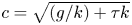 $c=\sqrt {(g/k)+\tau k}$ has a positive minimum, denoted by
  $c_{crit}$. For any fixed phase speed
  $c>c_{crit}$, there are two distinct positive wavenumbers satisfying the dispersion relation (1.1), denoted
  $k_1$ and
  $k_2$. Any travelling solution of the linearized problem with this speed can be expressed as a superposition of waves with these wavenumbers. If
  $k_1$ and
  $k_2$ are rationally related, the motion is spatially periodic and corresponds to the well-known Wilton ripples (Wilton Reference Wilton1915; Trichtchenko et al. Reference Trichtchenko, Deconinck and Wilkening2016; Akers et al. Reference Akers, Ambrose and Sulon2019; Akers & Nicholls Reference Akers and Nicholls2020). However, if
  $k_1$ and
  $k_2$ are irrationally related, the motion will be spatially quasi-periodic.
Recently, Berti & Montalto (Reference Berti and Montalto2016) and Baldi et al. (Reference Baldi, Berti, Haus and Montalto2018) have proved the existence of small-amplitude temporally quasi-periodic gravity–capillary standing waves using Nash–Moser theory. Using similar techniques, Berti, Franzoi & Maspero (Reference Berti, Franzoi and Maspero2020) have proved the existence of small-amplitude time quasi-periodic travelling gravity–capillary waves with constant vorticity; and Feola & Giuliani (Reference Feola and Giuliani2020) have proved existence of time quasi-periodic travelling gravity waves without surface tension or vorticity. Quasi-periodic travelling waves have a special meaning in the latter two papers that does not imply that they evolve without changing shape. All four papers formulate the problem on a spatially periodic domain, and it is shown that solutions of the linearized standing wave or travelling wave problems can be combined and perturbed to obtain temporally quasi-periodic solutions of the nonlinear problem. Following the same philosophy, we look for spatially quasi-periodic solutions of the travelling water wave equations that are perturbations of solutions of the linearized problem. The velocity potential can be eliminated from the Euler equations when looking for travelling solutions, so our goal is to study travelling waves with height functions of the form
 \begin{equation} \eta(\alpha) = \tilde\eta(k_1\alpha,k_2\alpha), \quad \tilde\eta(\alpha_1,\alpha_2)= \sum_{(\,j_1, j_2)\in\mathbb{Z}^2}\hat{\eta}_{j_1, j_2}\,\textrm{e}^{\textrm{i}(\,j_1\alpha_1+j_2\alpha_2)}. \end{equation}
Here,  $\tilde \eta$ is real valued and defined on the torus
 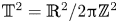 $\mathbb{T}^2=\mathbb{R}^2/2{\rm \pi} \mathbb{Z}^2$, and
  $\alpha$ parameterizes the free surface in such a way that the fluid domain is the image of the lower half-plane
  $\{w=\alpha +i\beta : \beta <0\}$ under a conformal map
  $z(w)$ whose imaginary part on the upper boundary is
 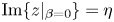 $\operatorname {Im}\{z\vert _{\beta =0}\}=\eta$. The leading term here is
  $\eta _{lin}(\alpha )=2\operatorname {Re}\{\hat \eta _{1,0}\,\textrm {e}^{\textrm {i}k_1\alpha }+ \hat \eta _{0,1}\,\textrm {e}^{\textrm {i}k_2\alpha }\}$, which will be a solution of the linearized problem.
Unlike Bridges & Dias (Reference Bridges and Dias1996), we use a conformal mapping formulation (Dyachenko et al. Reference Dyachenko, Kuznetsov, Spector and Zakharov1996a; Dyachenko, Zakharov & Kuznetsov Reference Dyachenko, Zakharov and Kuznetsov1996b; Choi & Camassa Reference Choi and Camassa1999; Dyachenko Reference Dyachenko2001; Zakharov, Dyachenko & Vasilyev Reference Zakharov, Dyachenko and Vasilyev2002; Li, Hyman & Choi Reference Li, Hyman and Choi2004; Hunter, Ifrim & Tataru Reference Hunter, Ifrim and Tataru2016; Dyachenko Reference Dyachenko2019) of the gravity–capillary water wave problem. This makes it possible to compute the normal velocity of the fluid from the velocity potential on the free surface via a quasi-periodic variant of the Hilbert transform. As in the periodic case, the Hilbert transform is a Fourier multiplier operator, but now acts on functions defined on a higher-dimensional torus. In a companion paper (Wilkening & Zhao Reference Wilkening and Zhao2020), we use this idea to develop a numerical method to compute the time evolution of solutions of the Euler equations from arbitrary quasi-periodic initial data. The present paper focuses on travelling waves in this framework.
We formulate the travelling wave computation as a nonlinear least-squares problem and use the Levenberg–Marquardt method to search for solutions. This approach builds on the overdetermined shooting methods developed by Wilkening and collaborators (Ambrose & Wilkening Reference Ambrose and Wilkening2010, Reference Ambrose and Wilkening2014; Wilkening & Yu Reference Wilkening and Yu2012; Rycroft & Wilkening Reference Rycroft and Wilkening2013; Govindjee, Potter & Wilkening Reference Govindjee, Potter and Wilkening2014) to compute standing waves and other time-periodic solutions. Specifically, we fix the ratio  $k_2/k_1$, denoted by
  $k$, and solve simultaneously for the phase speed
  $c$, the coefficient of surface tension
  $\tau$ and the unknown Fourier modes
  $\hat \eta _{j_1,j_2}$ in (1.2a,b) subject to the constraint that
  $\hat \eta _{1,0}$ and
  $\hat \eta _{0,1}$ have prescribed values. In § 3, we discuss the merits of these bifurcation parameters over, say, prescribing
  $\tau$ and
  $\hat \eta _{1,0}$ and solving for
  $\hat \eta _{0,1}$ along with
  $c$ and the other unknown Fourier modes. While the numerical method is general and can be used to search for solutions for any irrational
  $k$, for brevity we present results only for
  $k=1/\sqrt 2$ and
  $k = \sqrt {151}$, which exhibit clear nonlinear interaction between the two component waves.
Because we focus here on quasi-periodic travelling waves that persist to zero amplitude, the left and right branches of the dispersion relation (1.1) can be viewed as the wavenumbers of gravity waves and capillary waves, respectively (Djordjevic & Redekopp Reference Djordjevic and Redekopp1977). For the ocean, the ratio between them would be many orders of magnitude larger than we consider here, so our results pertain to much smaller-scale laboratory experiments rather than the ocean. Staying within the quasi-periodic Wilton ripple framework that begins at small amplitude with the dispersion relation (1.1) would be problematic for the ocean as increasing  $k$ to
  $10^7$ does not seem likely to lead to interesting nonlinear interactions between gravity and capillary waves due to their vast separation of scales, and is anyway computationally out of reach for our current algorithm.
A more promising idea is to look for spatially quasi-periodic gravity waves (with negligible surface tension) that bifurcate from finite-amplitude periodic travelling waves, similar to the wavelength doubling and tripling bifurcations found by Chen & Saffman (Reference Chen and Saffman1980). In this case, both component waves are gravity waves and the bifurcation arises due to a nonlinear resonance in the Euler equations. We have computed such a quasi-periodic bifurcation from the family of  $2{\rm \pi}$-periodic ‘pure gravity’ Stokes waves at a wave height of 0.809070794 and a wave speed of 1.083977047 when
  $k=1/\sqrt 2$. Details on these preliminary results will be given in future work. We also hope to extend our results to the case of finite-depth water waves, search for quasi-periodic perturbations of overhanging travelling gravity–capillary waves (Akers, Ambrose & Wright Reference Akers, Ambrose and Wright2014), and study the stability of these waves (Deconinck & Oliveras Reference Deconinck and Oliveras2011; Trichtchenko et al. Reference Trichtchenko, Deconinck and Wilkening2016).
The paper is organized as follows. In § 2, we define a quasi-periodic Hilbert transform, derive the equations of motion governing quasi-periodic travelling water waves and summarize the main results and notation introduced by Wilkening & Zhao (Reference Wilkening and Zhao2020) on the more general spatially quasi-periodic initial value problem. In § 3, we design a Fourier pseudo-spectral method to numerically solve the torus version of the quasi-periodic travelling wave equations. The discretization leads to an overdetermined nonlinear least-squares problem that we solve using a variant of the Levenberg–Marquardt method (Nocedal & Wright Reference Nocedal and Wright1999; Wilkening & Yu Reference Wilkening and Yu2012). In § 4, we present a detailed numerical study of a two-parameter family of quasi-periodic travelling waves with  $k=1/\sqrt 2$ and
  $g=1$ and validate the accuracy of the method. We then search for larger-amplitude waves with
  $k=1/\sqrt 2$ and
  $k=1/\sqrt {151}$ and explore the computational limits of our implementation. In the conclusion section, we summarize the results and discuss the effects of floating-point arithmetic and whether solutions might exist for rational values of
  $k$. Finally, in Appendix A, we study the dynamics of quasi-periodic travelling waves and show that the waves maintain a permanent form but generally travel at a non-uniform speed in conformal space in order to travel at constant speed in physical space.
2. Preliminaries
As explained above, the primary goal of this paper is to study spatially quasi-periodic travelling water waves using a conformal mapping framework. In this section, we establish notation; review the properties of the quasi-periodic Hilbert transform; discuss quasi-periodic conformal maps and complex velocity potentials; and propose a synthesis of viewpoints between the Hou, Lowengrub and Shelley formalism for evolving interfaces (Hou, Lowengrub & Shelley Reference Hou, Lowengrub and Shelley1994, Reference Hou, Lowengrub and Shelley1997) and the conformal mapping method developed by Dyachenko et al. (Reference Dyachenko, Kuznetsov, Spector and Zakharov1996a) and subsequent authors (Dyachenko et al. Reference Dyachenko, Zakharov and Kuznetsov1996b; Choi & Camassa Reference Choi and Camassa1999; Dyachenko Reference Dyachenko2001; Zakharov et al. Reference Zakharov, Dyachenko and Vasilyev2002; Dyachenko Reference Dyachenko2019). We also summarize the one-dimensional and torus versions of the equations of motion for the spatially quasi-periodic initial value problem (Wilkening & Zhao Reference Wilkening and Zhao2020); discuss families of one-dimensional quasi-periodic solutions corresponding to a single solution of the torus version of the problem; derive the equations governing travelling waves; and review the linear theory of quasi-periodic travelling waves.
2.1. Quasi-periodic functions and the Hilbert transform
A function  $u(\alpha )$ is quasi-periodic if there exists a continuous, periodic function
  $\tilde u(\boldsymbol \alpha )$ defined on the
  $d$-dimensional torus
  $\mathbb{T}^d$ such that
 \begin{equation} u(\alpha) = \tilde u(\boldsymbol{k} \alpha), \quad \tilde u(\boldsymbol\alpha) = \sum_{\boldsymbol{j}\in\mathbb{Z}^d}\hat{u}_{\boldsymbol{j}} \,\textrm{e}^{\textrm{i}\langle\,\boldsymbol{j},\,\boldsymbol{\alpha}\rangle}, \quad \alpha\in\mathbb{R}, \ \boldsymbol\alpha,\boldsymbol k \in \mathbb{R}^d. \end{equation}
We generally assume  $\tilde u(\boldsymbol \alpha )$ is real analytic, which means the Fourier modes satisfy the symmetry condition
  $\hat u_{-\boldsymbol j}=\overline {\hat u_{\boldsymbol j}}$ and decay exponentially as
  $|\,\boldsymbol j|\rightarrow \infty$, i.e.
  $|\hat u_{\boldsymbol j}|\le M\, \textrm {e}^{-\sigma |\,\boldsymbol j|}$ for some
  $M,\sigma >0$. Entries of the vector
  $\boldsymbol {k}$ are required to be linearly independent over
  $\mathbb {Z}$. Fixing this vector
  $\boldsymbol k$, we define two versions of the Hilbert transform, one acting on
  $u$ (the quasi-periodic version) and the other on
  $\tilde u$ (the torus version)
 \begin{equation} H[u](\alpha) = \frac{1}{\rm \pi}\operatorname{PV} \int_{-\infty}^\infty\frac{u(\xi)}{\alpha-\xi}\,\textrm{d} \xi, \quad H[\tilde u](\boldsymbol\alpha) = \sum_{\boldsymbol{j}\in\mathbb{Z}^d} ({-}i)\operatorname{sgn}(\langle\,\boldsymbol{j},\boldsymbol{k}\rangle) \hat{u}_{\boldsymbol{j}}\, \textrm{e}^{\textrm{i} \langle\,\boldsymbol{j},\,\boldsymbol{\alpha}\rangle}. \end{equation}
Here,  $\operatorname {sgn}(q)\in \{1,0,-1\}$ depending on whether
  $q>0$,
  $q=0$ or
  $q<0$, respectively. Note that the torus version of
  $H$ is a Fourier multiplier on
  $L^2(\mathbb{T}^d)$ that depends on
  $\boldsymbol k$. It is shown in Wilkening & Zhao (Reference Wilkening and Zhao2020) that
 \begin{equation} H[u](\alpha)=H[\tilde u](\boldsymbol k\alpha), \end{equation}
and the most general bounded analytic function  $f(w)$ in the lower half-plane whose real part agrees with
  $u$ on the real axis has the form
 \begin{equation} f(w) = \hat u_{\boldsymbol 0} + i\hat v_{\boldsymbol 0} + \sum_{\langle\,\boldsymbol j,\boldsymbol k\rangle<0} 2 \hat u_{\boldsymbol j}\,\textrm{e}^{\textrm{i}\langle\,\boldsymbol j,\boldsymbol k\rangle w}, \quad (w=\alpha+i\beta, \beta\le0), \end{equation}
where  $\hat v_{\boldsymbol 0}$ is an arbitrary constant and the sum is over all
  $\boldsymbol j\in \mathbb{Z}^d$ satisfying
  $\langle \,\boldsymbol j,\boldsymbol k\rangle <0$. The imaginary part of
  $f$ on the real axis is then given by
  $v=\hat v_{\boldsymbol 0}-H[u]$. Similarly, given
  $v$, the most general bounded analytic function
  $f(w)$ in the lower half-plane whose imaginary part agrees with
  $v$ on the real axis has the form (2.4) with
  $u=\hat u_{\boldsymbol 0} + H[v]$, where
  $\hat u_{\boldsymbol 0}$ is an arbitrary constant. This analytic extension is quasi-periodic on slices of constant depth, i.e.
 \begin{equation} f(w) = \tilde f(\boldsymbol k\alpha,\beta), \quad (w=\alpha+i\beta,\beta\le0), \end{equation}
where  $\tilde f(\boldsymbol \alpha ,\beta ) = \hat u_{\boldsymbol 0} + i\hat v_{\boldsymbol 0} + \sum _{\langle \,\boldsymbol j,\boldsymbol k\rangle <0} 2[\hat u_{\boldsymbol j}\, \textrm {e}^{-\langle \,\boldsymbol j,\boldsymbol k\rangle \beta }]\, \textrm {e}^{\textrm {i}\langle \,\boldsymbol j,\boldsymbol \alpha \rangle }$ is periodic in
  $\boldsymbol \alpha$ for fixed
  $\beta \le 0$. The torus version of the bounded analytic extension corresponding to
  $\tilde u(\boldsymbol \alpha +\boldsymbol \theta )$ is simply
  $\tilde f(\boldsymbol \alpha +\boldsymbol \theta ,\beta )$, which has imaginary part
  $\tilde v(\boldsymbol \alpha +\boldsymbol \theta )$ on the real axis. As a result, the Hilbert transform commutes with the shift operator,
 \begin{equation} H[\tilde u(\boldsymbol{\cdot}+\boldsymbol\theta)](\boldsymbol\alpha) = H[\tilde u](\boldsymbol\alpha+\boldsymbol\theta), \end{equation}
which can also be checked directly from (2.2a,b). We also define quasi-periodic and torus versions of two projection operators,
 \begin{equation} P = \operatorname{id} - P_0, \quad P_0 [u] = P_0 [\tilde u] = \hat{u}_{\boldsymbol{0}} = \frac{1}{(2{\rm \pi})^d} \int_{\mathbb{T}^d} \tilde u(\boldsymbol{\alpha})\, \textrm{d} \alpha_1\ldots \, \textrm{d} \alpha_d, \end{equation}
where  $P_0[u]$ is a constant function on
  $\mathbb{R}$,
  $P_0[\tilde u]$ is a constant function on
  $\mathbb{T}^d$ and
  $P[u]$ has zero mean on
  $\mathbb{R}$ in the sense that its torus representation,
  $P[\tilde u]$, which satisfies
  $P[u](\alpha )=P[\tilde u](\boldsymbol k\alpha )$, has zero mean on
  $\mathbb{T}^d$.
2.2. A quasi-periodic conformal mapping
For the general initial value problem (Wilkening & Zhao Reference Wilkening and Zhao2020), we consider a time-dependent conformal map  $z(w,t)$ that maps the lower half-plane
 \begin{equation} \mathbb{C}^{-} = \{w=\alpha+i\beta: \alpha\in\mathbb{R},\beta<0\} \end{equation}
to the fluid domain  $\varOmega _f(t)$ that lies below the free surface in physical space. At each time
  $t$, we assume
  $z(w,t)$ extends continuously to
  $\overline {\mathbb{C}^-}$, and in fact is analytic on a slightly larger half-plane
  $\mathbb{C}^-_\varepsilon =\{w: \operatorname {Im} w<\varepsilon \}$, where
  $\varepsilon >0$ could depend on
  $t$. The free surface
  $\varGamma (t)$ is parameterized by
 \begin{equation} \zeta(\alpha,t)=\xi(\alpha,t)+i\eta(\alpha,t), \quad (\alpha\in\mathbb{R}, t \,{fixed}), \quad \zeta = z\vert_{\beta=0}. \end{equation}
We assume  $\alpha \mapsto \zeta (\alpha ,t)$ is injective but do not assume
  $\varGamma (t)$ is the graph of a single-valued function of
  $x$ in the derivation. An example of a time-dependent spatially quasi-periodic overturning water wave is computed by Wilkening & Zhao (Reference Wilkening and Zhao2020). In future work we will study travelling quasi-periodic perturbations of the overhanging periodic travelling water waves computed by Akers et al. (Reference Akers, Ambrose and Wright2014).
The conformal map is required to remain a bounded distance from the identity map in the lower half-plane. Specifically, we require that
 \begin{equation} |z(w,t)-w|\le M(t) \quad (w=\alpha+i\beta, \beta\le0), \end{equation}
where  $M(t)$ is a uniform bound that could vary in time. The Cauchy integral formula implies that
  $|z_w-1|\le M(t)/|\beta |$, so at any fixed time,
 \begin{equation} z_w\rightarrow1 \text{ as } \beta\to-\infty. \end{equation}
In this paper and its companion (Wilkening & Zhao Reference Wilkening and Zhao2020), we assume  $\eta$ has two spatial quasi-periods, i.e. at any time it has the form (2.1a,b) with
  $d=2$ and
  $\boldsymbol {k}=[k_1,k_2]^T$. This is a major departure from previous work (Meiron, Orszag & Israeli Reference Meiron, Orszag and Israeli1981; Dyachenko et al. Reference Dyachenko, Kuznetsov, Spector and Zakharov1996a; Zakharov et al. Reference Zakharov, Dyachenko and Vasilyev2002; Dyachenko, Lushnikov & Korotkevich Reference Dyachenko, Lushnikov and Korotkevich2016), where
  $\eta$ is assumed to be periodic. Through non-dimensionalization, we may set
  $k_1=1$ and
  $k_2 = k$, where
  $k$ is irrational
 \begin{equation} \eta(\alpha,t) = \tilde\eta(\alpha,k\alpha,t), \quad \tilde\eta(\alpha_1,\alpha_2,t) = \sum_{j_1, j_2\in\mathbb{Z}} \hat{\eta}_{j_1, j_2}(t)\,\textrm{e}^{\textrm{i}(\,j_1\alpha_1+j_2\alpha_2)}. \end{equation}
Here,  $\hat {\eta }_{-j_1, -j_2}(t) = \overline {\hat {\eta }_{j_1,j_2}(t)}$ since
  $\tilde \eta (\alpha _1,\alpha _2,t)$ is real valued. Since
  $w\mapsto [z(w,t)-w]$ is bounded and analytic on
  $\mathbb{C}^-$ and its imaginary part agrees with
  $\eta$ on the real axis, there is a real number
  $x_0$ (possibly depending on time) such that
 \begin{equation} \xi(\alpha, t) = \alpha + x_0(t) + H[\eta](\alpha, t), \quad \xi_\alpha(\alpha, t) = 1 + H[\eta_\alpha](\alpha, t). \end{equation}
We use a tilde to denote the periodic functions on the torus that correspond to the quasi-periodic parts of  $\xi$,
  $\zeta$ and
  $z$,
$z$,
 \begin{equation} \left. \begin{gathered} \xi(\alpha,t) = \alpha + \tilde\xi(\alpha,k\alpha,t), \quad \zeta(\alpha,t) = \alpha + \tilde\zeta(\alpha,k\alpha,t), \\ z(\alpha+i\beta,t)=(\alpha+i\beta )+ \tilde z(\alpha,k\alpha,\beta,t), \quad (\beta\le 0). \end{gathered} \right\} \end{equation}
Specifically,  $\tilde \xi = x_0(t) + H[\tilde \eta ]$,
  $\tilde \zeta = \tilde \xi + i\tilde \eta$, and
 \begin{equation} \tilde z(\alpha_1,\alpha_2,\beta,t) = x_0(t)+i\hat\eta_{0,0}(t)+\sum_{j_1+j_2k<0} (2i\hat\eta_{j_1,j_2}(t)\, \textrm{e}^{-(\,j_1+j_2k)\beta}) \, \textrm{e}^{\textrm{i}(\,j_1\alpha_1+j_2\alpha_2)}. \end{equation}
Since the modes  $\hat \eta _{j_1,j_2}$ are assumed to decay exponentially, there is a uniform bound
  $M(t)$ such that
  $|\tilde z(\alpha _1,\alpha _2,\beta ,t)|\le M(t)$ for
  $(\alpha _1,\alpha _2)\in \mathbb{T}^2$ and
  $\beta \le 0$. Wilkening & Zhao (Reference Wilkening and Zhao2020) show that as long as the free surface
  $\zeta (\alpha ,t)$ does not self-intersect at a given time
  $t$, the mapping
  $w\mapsto z(w,t)$ is an analytic isomorphism of the lower half-plane onto the fluid region.
2.3. The complex velocity potential and equations of motion for the initial value problem
Adopting the notation of Wilkening & Zhao (Reference Wilkening and Zhao2020), let  $\varPhi ^{phys}(x,y,t)$ denote the velocity potential in physical space and let
  $W^{phys}(x+iy,t)= \varPhi ^{phys}(x,y,t)+i\varPsi ^{phys}(x,y,t)$ denote the complex velocity potential, where
  $\varPsi ^{phys}$ is the streamfunction. Using the conformal mapping
  $z(w,t)$, we pull back these functions to the lower half-plane and define
 \begin{equation} W(w,t) = \varPhi(\alpha,\beta,t)+i\varPsi(\alpha,\beta,t) = W^{phys}(z(w,t),t), \quad (w=\alpha+i\beta). \end{equation}
We also define
 \begin{equation} \varphi=\varPhi\vert_{\beta=0}, \quad \psi=\varPsi\vert_{\beta=0}. \end{equation}
We assume  $\varphi$ is quasi-periodic with the same quasi-periods as
  $\eta$,
 \begin{equation} \varphi(\alpha, t) = \tilde\varphi(\alpha,k\alpha,t), \quad \tilde\varphi(\alpha_1,\alpha_2,t) = \sum_{j_1, j_2\in\mathbb{Z}} \hat{\varphi}_{j_1, j_2}(t) \, \textrm{e}^{\textrm{i}(\,j_1\alpha_1+j_2\alpha_2)}. \end{equation}
The fluid velocity  $\boldsymbol {\nabla }\varPhi ^{phys}(x,y,t)$ is assumed to decay to zero as
  $y\rightarrow -\infty$ (since we work in the laboratory frame). Since
  $\textrm {d} W/ \textrm {d} w=(\textrm {d} W^{phys}/\textrm {d} z)(\textrm {d} z/ \textrm {d} w)$, it follows from (2.11) that
  $\textrm {d} W/ \textrm {d} w\rightarrow 0$ as
  $\beta \to -\infty$. Thus,
 \begin{equation} \psi_\alpha ={-}H[\varphi_\alpha], \quad \psi(\alpha, t) ={-}H[\varphi](\alpha, t). \end{equation}
Here, we have assumed  $P_0[\varphi ] = \hat {\varphi }_{0,0}(t) = 0$ and
  $P_0[\psi ] = \hat {\psi }_{0,0}(t) = 0$, which is allowed since
  $\varPhi$ and
  $\varPsi$ can be modified by additive constants (or functions of time only) without affecting the fluid motion.
Let  $U$ and
  $V$ denote the normal and tangential velocities of the curve parameterization, respectively; let
  $s_\alpha =|\zeta _\alpha |=(\xi _\alpha ^2+\eta _\alpha ^2)^{1/2}$ denote the rate at which arclength increases as the curve
  $\alpha \mapsto \zeta (\alpha ,t)$ is traversed; and let
  $\theta$ denote the tangent angle of the curve relative to the horizontal. Then
 \begin{equation} \zeta_\alpha = s_\alpha\, \textrm{e}^{\textrm{i}\theta}, \quad \zeta_t = (V+iU)\,\textrm{e}^{\textrm{i}\theta}. \end{equation}
Tracking a fluid particle  $x_p(t)+iy_p(t)= \zeta (\alpha _p(t),t)$ on the free surface, we find that
 \begin{equation} \dot x_p=\xi_\alpha\dot\alpha_p+\xi_t=\varPhi^{phys}_x, \quad \dot y_p=\eta_\alpha\dot\alpha_p+\eta_t=\varPhi^{phys}_y. \end{equation}
Eliminating  $\dot \alpha _p$ gives the kinematic condition
 \begin{equation} U = \zeta_t\boldsymbol{\cdot}\hat{\boldsymbol n} = \boldsymbol{\nabla}\varPhi^{phys}\boldsymbol{\cdot}\hat{\boldsymbol n}, \end{equation}
where  $\hat {\boldsymbol n}=(-\eta _\alpha ,\xi _\alpha )/s_\alpha$ is the outward unit normal to
  $\varGamma$ and we have identified
  $\zeta _t$ with the vector
  $(\xi _t,\eta _t)$ in
  $\mathbb{R}^2$. The general philosophy proposed by Hou, Lowengrub & Shelley (HLS) (Hou et al. Reference Hou, Lowengrub and Shelley1994, Reference Hou, Lowengrub and Shelley1997) is that while (2.22) constrains the normal velocity
  $U$ of the curve to match that of the fluid, the tangential velocity
  $V$ can be chosen arbitrarily to improve the mathematical properties of the representation or the accuracy and stability of the numerical scheme. Whereas HLS propose choosing
  $V$ to keep
  $s_\alpha (t)$ independent of
  $\alpha$, we interpret the work of Dyachenko et al. (Reference Dyachenko, Kuznetsov, Spector and Zakharov1996a) and subsequent authors (Choi & Camassa Reference Choi and Camassa1999; Dyachenko Reference Dyachenko2001, Reference Dyachenko2019; Zakharov et al. Reference Zakharov, Dyachenko and Vasilyev2002) as choosing
  $V$ to maintain a conformal representation. Briefly, since
  $\varPhi ^{phys}$ and
  $\varPsi ^{phys}$ satisfy the Cauchy–Riemann equations, we have
 \begin{equation} -\frac{\psi_\alpha}{s_\alpha} ={-}\frac{\varPsi^{phys}_x\xi_\alpha + \varPsi^{phys}_y\eta_\alpha}{s_\alpha} = \frac{\varPhi^{phys}_y\xi_\alpha - \varPhi^{phys}_x\eta_\alpha}{s_\alpha} = \boldsymbol{\nabla}\varPhi^{phys}\boldsymbol{\cdot} \hat{\boldsymbol n} = U. \end{equation}
Assuming  $z_t/z_\alpha$ is bounded and analytic in the lower half-plane (justified below),
 \begin{equation} \left. \frac{z_t}{z_\alpha}\right\vert_{\beta=0} = \frac{\zeta_t}{\zeta_\alpha} = \frac{V+iU}{s_\alpha} \Rightarrow \frac{V}{s_\alpha} = H\left(\frac{U}{s_\alpha}\right)+C_1 ={-}H\left(\frac{\psi_\alpha}{s_\alpha^2}\right)+C_1, \end{equation}
where  $C_1$ is an arbitrary constant (in space) that we are free to choose. For any differentiable function
  $\alpha _0(t)$, replacing
  $C_1(t)$ by
 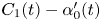 $C_1(t)-\alpha _0'(t)$ will cause a reparameterization of the solution with
  $\alpha$ replaced by
  $\alpha -\alpha _0(t)$; see Appendix A. The tangential and normal velocities can be rotated back to obtain
  $\xi _t$ and
  $\eta _t$ via
 \begin{equation} \begin{pmatrix} \xi_t \\ \eta_t \end{pmatrix} = \begin{pmatrix} \xi_\alpha & -\eta_\alpha \\ \eta_\alpha & \xi_\alpha \end{pmatrix} \begin{pmatrix} V/s_\alpha \\ U/s_\alpha \end{pmatrix}, \end{equation}
which can be interpreted as the real and imaginary parts of the complex multiplication  $\zeta _t = (\zeta _\alpha )(\zeta _t/\zeta _\alpha )$. As explained in Wilkening & Zhao (Reference Wilkening and Zhao2020), the first equation of (2.25) is automatically satisfied if the second equation holds and
  $\xi$ is reconstructed from
  $\eta$ via (2.13a,b), provided
  $x_0(t)$ satisfies
 \begin{equation} \frac{\textrm{d}\kern0.7pt x_0}{\textrm{d} t} = P_0\left[ \xi_\alpha \frac V{s_\alpha} - \eta_\alpha \frac U{s_\alpha} \right]. \end{equation}
The equations of motion for water waves in the conformal framework may now be written
 \begin{equation} \left. \begin{gathered}
\xi_\alpha = 1 + H[\eta_\alpha], \quad \psi ={-}H[\varphi],
\quad J = \xi_\alpha^2 + \eta_\alpha^2, \quad \chi =
\dfrac{\psi_\alpha}{J}, \\
\text{choose }C_1 \text{ (see below), compute }
\dfrac{\textrm{d}\kern0.7pt x_0}{\textrm{d} t} \text{ in (2.26)} \text{ if necessary},\\
\eta_t ={-}\eta_\alpha H[\chi] - \xi_\alpha\chi + C_1\eta_\alpha, \quad \kappa =
\dfrac{\xi_\alpha\eta_{\alpha\alpha} -
\eta_\alpha\xi_{\alpha\alpha}}{J^{3/2}}, \\ \varphi_t =
P\left[\dfrac{\psi_\alpha^2 - \varphi_\alpha^2}{2J} -
\varphi_\alpha H[\chi] + C_1\varphi_\alpha - g\eta +
\tau\kappa\right], \end{gathered} \right\}
\end{equation}
\begin{equation} \left. \begin{gathered}
\xi_\alpha = 1 + H[\eta_\alpha], \quad \psi ={-}H[\varphi],
\quad J = \xi_\alpha^2 + \eta_\alpha^2, \quad \chi =
\dfrac{\psi_\alpha}{J}, \\
\text{choose }C_1 \text{ (see below), compute }
\dfrac{\textrm{d}\kern0.7pt x_0}{\textrm{d} t} \text{ in (2.26)} \text{ if necessary},\\
\eta_t ={-}\eta_\alpha H[\chi] - \xi_\alpha\chi + C_1\eta_\alpha, \quad \kappa =
\dfrac{\xi_\alpha\eta_{\alpha\alpha} -
\eta_\alpha\xi_{\alpha\alpha}}{J^{3/2}}, \\ \varphi_t =
P\left[\dfrac{\psi_\alpha^2 - \varphi_\alpha^2}{2J} -
\varphi_\alpha H[\chi] + C_1\varphi_\alpha - g\eta +
\tau\kappa\right], \end{gathered} \right\}
\end{equation}
where the last equation comes from the unsteady Bernoulli equation and the Laplace–Young condition for the pressure. These equations govern the evolution of  $x_0$,
  $\eta$ and
  $\varphi$. The full curve
  $\zeta =\xi +i\eta$ and its analytic extension
  $z$ to the lower half-plane can be reconstructed from
  $\eta$ using (2.13a,b) and (2.14). Doing so ensures that
  $z$ is injective and that
  $z_t/z_\alpha$ remains bounded in the lower half-plane provided that the free surface does not self-intersect and
  $J$ remains non-zero on the surface; see Wilkening & Zhao (Reference Wilkening and Zhao2020) for details.
As noted by Wilkening & Zhao (Reference Wilkening and Zhao2020), (2.27) can be interpreted as an evolution equation for the functions  $\tilde \zeta (\alpha _1,\alpha _2,t)$ and
  $\tilde \varphi (\alpha _1,\alpha _2,t)$ on the torus
  $\mathbb{T}^2$. The
  $\alpha$-derivatives are replaced by the directional derivatives
  $[\partial _{\alpha _1}+k\partial _{\alpha _2}]$ and the quasi-periodic Hilbert transform is replaced by its torus version, i.e.
  $H[\tilde u]$ in (2.2a,b) above. The pseudo-spectral method proposed in Wilkening & Zhao (Reference Wilkening and Zhao2020) is based on this representation. A convenient choice of
  $C_1$ is
 \begin{equation} C_1 = \left[H\left(\frac{\tilde\psi_\alpha}{\tilde J}\right) - \frac{\tilde\eta_\alpha\tilde\psi_\alpha}{ (1+\tilde\xi_\alpha)\tilde J} \right]_{(\alpha_1,\alpha_2)=(0,0)}, \end{equation}
which causes  $\tilde \xi (0,0,t)$ to remain constant in time, alleviating the need to evolve
  $x_0(t)$ explicitly. Here
  $\tilde J=(1+\tilde \xi _\alpha )^2 + \tilde \eta _\alpha ^2$, and all instances of
  $\xi _\alpha$ in (2.27) must be replaced by
 \begin{equation} \widetilde{\xi_\alpha} = 1 + \tilde\xi_\alpha, \end{equation}
since the secular growth term  $\alpha$ is not part of
  $\tilde \xi$ in (2.14). Using (2.13a,b) and (2.14),
  $\tilde \zeta$ is completely determined by
  $x_0(t)$ and
  $\tilde \eta$, so only these have to be evolved – the formula for
  $\tilde \xi _t$ in (2.25) is redundant as long as (2.26) is satisfied. Other choices of
  $C_1$ are considered in Appendix A.
Wilkening & Zhao (Reference Wilkening and Zhao2020) show that solving the torus version of (2.27) yields a three-parameter family of one-dimensional solutions of the form
 \begin{equation} \begin{aligned} \zeta(\alpha,t; \theta_1,\theta_2,\delta) & = \alpha + \delta + \tilde\zeta( \theta_1+\alpha,\theta_2+k\alpha,t), \\ \varphi(\alpha,t; \theta_1,\theta_2) & = \tilde\varphi( \theta_1+\alpha,\theta_2+k\alpha,t), \end{aligned} \quad \left( \begin{aligned} \alpha\in\mathbb{R}, \ t\ge0 \\ \theta_1,\theta_2,\ \delta\in\mathbb{R} \end{aligned}\right). \end{equation}
The parameters  $(\theta _1,\theta _2,\delta )$ lead to the same solution as
  $(0,\theta _2-k\theta _1,0)$ up to a spatial phase shift and
  $\alpha$-reparameterization. Thus, every solution is equivalent to one of the form
 \begin{equation} \begin{aligned} \zeta(\alpha,t; 0,\theta,0) & = \alpha + \tilde\zeta(\alpha,\theta+k\alpha,t), \\ \varphi(\alpha,t; 0,\theta) & = \tilde\varphi(\alpha,\theta+k\alpha,t) \end{aligned} \quad \alpha\in\mathbb{R}, \ t\ge 0,\ \theta\in[0,2{\rm \pi}). \end{equation}
Within this smaller family, two values of  $\theta$ lead to equivalent solutions if they differ by
  $2{\rm \pi} (n_1k+n_2)$ for some integers
  $n_1$ and
  $n_2$. This equivalence is due to solutions ‘wrapping around’ the torus with a spatial shift,
 \begin{align} \zeta(\alpha+2{\rm \pi} n_1,t; 0,\theta,0) = \zeta(\alpha,t; 0,\theta+2{\rm \pi}(n_1k+n_2),2{\rm \pi} n_1), \quad (\alpha\in[0,2{\rm \pi}),\ n_1\in\mathbb{Z}). \end{align}
Here,  $n_2$ is chosen so that
  $0\le [\theta +2{\rm \pi} (n_1k+n_2)]<2{\rm \pi}$ and we used periodicity of
  $\zeta (\alpha ,t; \theta _1,\theta _2,\delta )$ with respect to
  $\theta _1$ and
  $\theta _2$. Wilkening & Zhao (Reference Wilkening and Zhao2020) also show that if all the waves in the family (2.31) are single valued and have no vertical tangent lines, there is a corresponding family of solutions of the Euler equations in a standard graph-based formulation (Zakharov Reference Zakharov1968; Craig & Sulem Reference Craig and Sulem1993; Johnson Reference Johnson1997) that are quasi-periodic in physical space.
2.4. Quasi-periodic travelling water waves
We now specialize to the case of quasi-periodic travelling waves and derive the equations of motion in a conformal mapping framework. One approach (see e.g. Milewski et al. (Reference Milewski, Vanden-Broeck and Wang2010) for the periodic case) is to write down the equations of motion in a graph-based representation of the surface variables  $\eta ^{phys}(x,t)$ and
  $\varphi ^{phys}(x,t)=\varPhi ^{phys}(x,\eta (x,t),t)$ and substitute
 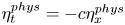 $\eta ^{phys}_t = -c\eta ^{phys}_x$,
  $\varphi ^{phys}_t = -c\varphi ^{phys}_x$ to solve for the initial condition of a solution of the form
 \begin{equation} \eta^{phys}(x,t)=\eta^{phys}_0(x-ct), \quad \varphi^{phys}(x,t)=\varphi^{phys}_0(x-ct). \end{equation}
We present below an alternative derivation of the equations in Milewski et al. (Reference Milewski, Vanden-Broeck and Wang2010) that is more direct and does not assume the wave profile is single valued. Other systems of equations have also been derived to describe travelling water waves, e.g. by Nekrasov (Reference Nekrasov1921), Milne-Thomson (Reference Milne-Thomson1968) and Dyachenko et al. (Reference Dyachenko, Lushnikov and Korotkevich2016).
Recall the kinematic condition (2.23) that the normal velocity of the curve is given by 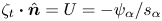 $\zeta _t\boldsymbol {\cdot }\hat {\boldsymbol n} = U = -\psi _\alpha /s_\alpha$. Since the wave travels at constant speed
  $c$ in physical space, there is a reparameterization
  $\beta (\alpha ,t)$ such that
 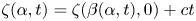 $\zeta (\alpha ,t)=\zeta (\beta (\alpha ,t),0)+ct$. Since
  $\zeta _\alpha$ is tangent to the curve, the normal velocity is simply
  $\zeta _t\boldsymbol {\cdot }\hat {\boldsymbol n}=(c,0)\boldsymbol {\cdot }\hat {\boldsymbol n}=-c\eta _\alpha /s_\alpha$, where we used
 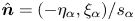 $\hat {\boldsymbol n}=(-\eta _\alpha ,\xi _\alpha )/s_\alpha$. We conclude that
 \begin{equation} \psi_\alpha = c\eta_\alpha, \quad \varphi_\alpha = H[\psi_\alpha] = cH[\eta_\alpha] = c(\xi_\alpha -1). \end{equation}
This expresses  $\psi$ and
  $\varphi$ (up to additive constants) in terms of
  $\eta$ and
  $\xi =\alpha +x_0+H[\eta ]$, leaving only
  $\eta$ to be determined. As in the graph-based approach of (2.33a,b) above, it suffices to compute the initial wave profile at
  $t=0$ to know the full evolution of the travelling wave under (2.27); however, the wave generally travels at a non-uniform speed in conformal space in order to travel at constant speed in physical space. This is demonstrated in § 4.2 and proved in Appendix A.
The two-dimensional velocity potential  $\varPhi ^{phys}(x,y,t)$ may be assumed to exist even if the travelling wave possesses overhanging regions that cause the graph-based representation via
  $\eta ^{phys}(x,t)$ and
  $\varphi ^{phys}(x,t)$ to break down. In a moving frame travelling at constant speed
  $c$ along with the wave, the free surface will be a streamline. Let
  $\breve{z}=z-ct$ denote position in the moving frame and note that the complex velocity potential picks up a background flow term,
  $\breve{W}^{phys}(\breve{z},t)=W^{phys}(\breve{z}+ct,t)-c\breve{z}$, and becomes time independent. We drop
  $t$ in the notation and define
  $\breve{W}(w)=\breve{W}^{phys}(\breve{z}(w))$, where
  $\breve{z}(w)=z(w,0)$ conformally maps the lower half-plane onto the fluid region of this stationary problem. We assume
  $W^{phys}(\breve{z}(\alpha ),0)$ is quasi-periodic with exponentially decaying mode amplitudes, so
 \begin{equation} |\breve{W}(w)+cw|\le|W^{phys}(\breve{z}(w),0)|+c|\breve{z}(w)-w|,
\end{equation}
\begin{equation} |\breve{W}(w)+cw|\le|W^{phys}(\breve{z}(w),0)|+c|\breve{z}(w)-w|,
\end{equation}
is bounded in the lower half-plane. Since the streamfunction  $\operatorname {Im}\{\breve{W}^{phys}(\breve{z})\}$ is constant on the free surface, we may assume
 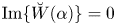 $\operatorname {Im}\{\breve{W}(\alpha )\}=0$ for
  $\alpha \in \mathbb{R}$. The function
  $\operatorname {Im}\{\breve{W}(w)+cw\}$ is then bounded and harmonic in the lower half-plane and satisfies homogeneous Dirichlet boundary conditions on the real line, so it is zero (Axler, Bourdon & Ramey Reference Axler, Bourdon and Ramey1992). Up to an additive real constant,
 \begin{equation} \breve{W}(w)={-}cw. \end{equation}
Thus,  $|\breve{\boldsymbol {\nabla }}\breve{\varPhi} ^{phys}|^2=|\breve{W}'(w)/\breve{z}'(w)|^2=c^2/J$. Since the free surface is a streamline in the moving frame, the steady Bernoulli equation
 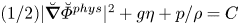 $(1/2)|\breve{\boldsymbol {\nabla }}\breve{\varPhi}^{phys}|^2+g\eta +p/\rho =C$ together with the Laplace–Young condition
  $p=p_0-\rho \tau \kappa$ on the pressure gives
 \begin{equation} \left. \begin{gathered} \xi_\alpha = 1 + H[\eta_\alpha], \quad J = \xi_\alpha^2 + \eta_\alpha^2, \\ \kappa = \dfrac{\xi_\alpha\eta_{\alpha\alpha} - \eta_\alpha\xi_{\alpha\alpha}}{J^{3/2}}, \quad P\left[\dfrac{c^2}{2J} + g\eta -\tau\kappa\right] = 0, \end{gathered}\right\} \end{equation}
which is the desired system of equations for  $\eta$.
In the quasi-periodic travelling wave problem, we seek a solution of (2.37) of the form (2.12a,b), except that  $\tilde \eta$ and its Fourier modes will not depend on time. Like the initial value problem, (2.37) can be interpreted as a nonlinear system of equations for
  $\tilde \eta (\alpha _1,\alpha _2)$ defined on
  $\mathbb{T}^2$, where the
  $\alpha$-derivatives are replaced by
  $[\partial _{\alpha _1} + k\partial _{\alpha _2}]$ and the Hilbert transform is replaced by its torus version in (2.2a,b). Without loss of generality, we assume
 \begin{equation} \hat{\eta}_{0,0} = 0. \end{equation}
We also assume that  $\tilde \eta$ is an even, real function of
  $(\alpha _1,\alpha _2)$ on
  $\mathbb{T}^2$. Hence, in our set-up, the Fourier modes of
  $\tilde \eta$ satisfy
 \begin{equation} \hat{\eta}_{{-}j_1, -j_2} = \bar{\hat{\eta}}_{j_1, j_2}, \quad \hat{\eta}_{{-}j_1, -j_2} = \hat{\eta}_{j_1, j_2}, \quad (\,j_1, j_2)\in \mathbb{Z}^2. \end{equation}
This implies that all the Fourier modes  $\hat {\eta }_{j_1, j_2}$ are real, and causes
 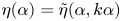 $\eta (\alpha )=\tilde \eta (\alpha ,k\alpha )$ to be even as well, which is compatible with the symmetry of (2.37). However, as in (2.30), there is a larger family of quasi-periodic travelling solutions embedded in this solution, namely
 \begin{equation} \eta(\alpha;\theta) = \tilde\eta(\alpha,\theta+k\alpha). \end{equation}
As in (2.32), two values of  $\theta$ lead to equivalent solutions (up to
  $\alpha$-reparameterization and a spatial phase shift) if they differ by
  $2{\rm \pi} (n_1k+n_2)$ for some integers
  $n_1$ and
  $n_2$. In general,
  $\eta (\alpha -\alpha _0;\theta )$ will not be an even function of
  $\alpha$ for any choice of
  $\alpha _0$ unless
 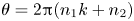 $\theta =2{\rm \pi} (n_1k+n_2)$ for some integers
  $n_1$ and
  $n_2$. In the periodic case, symmetry breaking travelling water waves have been found by Zufiria (Reference Zufiria1987), though most of the literature is devoted to periodic travelling waves with even symmetry.
2.5. Linear theory of quasi-periodic travelling waves
Linearizing (2.37) around the trivial solution  $\eta (\alpha ) = 0$, we obtain,
 \begin{equation} c^2H[\delta{\eta}_\alpha] - g\delta{\eta} + \tau\delta{\eta}_{\alpha\alpha} = 0, \end{equation}
where  $\delta \eta$ denotes the variation of
  $\eta$. Substituting (1.2a,b) into (2.41), we obtain a resonance relation for the Fourier modes of
  $\delta \eta$
 \begin{equation} (c^2|\,j_1k_1+j_2k_2| - g - \tau(\,j_1k_1+j_2k_2)^2) \widehat{\delta\eta}_{j_1,j_2} = 0, \quad (\,j_1, j_2) \in \mathbb{Z}^2. \end{equation}
Note that,  $j_1k_1+j_2k_2$, which appears in the exponent of the Fourier plane wave representation (1.2a,b), plays the role of
  $k$ in the dispersion relation (1.1). Many families of quasi-periodic travelling wave solutions bifurcate from the trivial solution even after specifying
  $k_1$ and
  $k_2$. Selecting a branch amounts to choosing two of the modes
  $\widehat {\delta \eta }_{j_1,j_2}$ to bring in at linear order and setting the others to zero in (2.42). In this paper, we focus on the case in which
  $\hat \eta _{1,0}$ and
  $\hat \eta _{0,1}$ enter linearly. This gives the first-order resonance conditions
 \begin{equation} c^2k_1 - g - \tau k_1^2 = 0, \quad c^2k_2 - g - \tau k_2^2 = 0, \end{equation}
where  $k_1=1$ and
  $k_2=k$ in our non-dimensionalized setting. For right-moving waves, we then have
  $c=\sqrt {g/k_1 + g/k_2}$ and
  $\tau =g/(k_1k_2)$. Any superposition of waves with dimensionless wave numbers
  $k_1=1$ and
  $k_2=k$ travelling with speed
  $c=c_{lin}$ will solve the linearized problem (2.41) for
  $\tau =\tau _{lin}$. Here, we have introduced the notation
  $c_{lin}=\sqrt {g+g/k}$ and
  $\tau _{lin}=g/k$ to facilitate the discussion of nonlinear effects below.
3. Numerical method
Equations (2.37) involve computing derivatives and Hilbert transforms of quasi-periodic functions that arise in intermediate computations. Let  $f(\alpha )$ denote one of these functions, and let
  $\tilde f$ denote the corresponding periodic function on the torus,
 \begin{equation} f(\alpha) = \tilde f(\alpha,k\alpha), \quad \tilde f(\alpha_1,\alpha_2) = \sum_{j_1, j_2 \in \mathbb{Z}} \hat{f}_{j_1, j_2}\, \textrm{e}^{\textrm{i}(\,j_1\alpha_1+j_2\alpha_2)}, \quad (\alpha_1, \alpha_2)\in\mathbb{T}^2. \end{equation}
Each  $\tilde f$ that arises is represented by its values on a uniform
  $M_1\times M_2$ grid on the torus
  $\mathbb{T}^2$,
 \begin{equation} \tilde f_{m_1,m_2} = \tilde f(2{\rm \pi} m_1/M_1, 2{\rm \pi} m_2/M_2), \quad (0\le m_1 < M_1, 0\le m_2 < M_2). \end{equation}
Products, powers and quotients in (2.37) are evaluated pointwise on the grid while derivatives and the Hilbert transform are computed in Fourier space via
 \begin{equation} \left. \begin{gathered} \widetilde{f_\alpha} (\alpha_1, \alpha_2) = \sum_{j_1, j_2\in \mathbb{Z}} i(\,j_1 + j_2 k) \hat{f}_{j_1, j_2}\, \textrm{e}^{\textrm{i}(\,j_1\alpha_1+j_2\alpha_2)}, \\ \widetilde{H[f]} (\alpha_1, \alpha_2) = \sum_{j_1, j_2\in \mathbb{Z}} ({-}i)\text{sgn}(\,j_1 + j_2 k) \hat{f}_{j_1, j_2} \, \textrm{e}^{\textrm{i}(\,j_1\alpha_1+j_2\alpha_2)}. \end{gathered}\right\} \end{equation}
We use the ‘r2c’ version of the two-dimensional fast Fourier transform (FFTW) library to rapidly compute the forward and inverse transform given by
 \begin{align} \hat f_{j_1,j_2} = \frac1{M_2}\sum_{m_2=0}^{M_2-1} \left(\frac1{M_1}\sum_{m_1=0}^{M_1-1} \tilde f_{m_1,m_2} \, \textrm{e}^{{-}2{\rm \pi} {\rm i}j_1m_1/M_1}\right)\, \textrm{e}^{{-}2{\rm \pi} {\rm i}j_2m_2/M_2}, \quad \begin{pmatrix} 0\le j_1\le M_1/2 \\ -M_2/2< j_2\le M_2/2 \end{pmatrix}. \end{align}
The FFTW library actually returns the index range  $0\le j_2 < M_2$, but we use
  $\hat f_{j_1,j_2-M_2}=\hat f_{j_1,j_2}$ to de-alias the Fourier modes and map the indices
  $j_2>M_2/2$ to their correct negative values. The missing entries with
  $-M_1/2 < j_1 < 0$ are determined implicitly by
 \begin{equation} \hat f_{{-}j_1,-j_2}=\overline{\hat f_{j_1,j_2}}. \end{equation}
When computing  $f_\alpha$ and
  $H[f]$ via (3.3), the Nyquist modes with
  $j_1=M_1/2$ or
  $j_2=M_2/2$ are set to zero, which ensures that the ‘c2r’ transform reconstructs real-valued functions
  $\widetilde {f_\alpha }$ and
  $\widetilde {H[f]}$ from their Fourier modes. Further details on this pseudo-spectral representation are given in Wilkening & Zhao (Reference Wilkening and Zhao2020) in the context of time stepping the dynamic equations (2.27).
This pseudo-spectral representation of quasi-periodic functions can be generalized to functions with quasi-periods larger than two. In this case, one could still use the ’r2c’ and ’c2r’ routines in the FFTW library where the function is represented by a  $d$-dimensional array of Fourier coefficients
 \begin{equation} \tilde{f}_{m_1, m_2, \ldots, m_d} = \sum_{j_1=0}^{M_1-1} \cdots \sum_{j_d=0}^{M_d-1} \hat{f}_{j_1, j_2, \ldots, j_d} \, \textrm{e}^{2{\rm \pi} {\rm i} j_dm_d/M_d} \ldots \textrm{e}^{2{\rm \pi} {\rm i} j_1m_1/M_1}, \end{equation}
where  $\tilde {f}_{m_1, m_2, \ldots , m_d}=\tilde f(2{\rm \pi} m_1/M_1,\ldots ,2{\rm \pi} m_d/M_d)$ is the value of
  $\tilde {f}$ evaluated on a uniform
  $M_1\times M_2\times \cdots \times M_d$ grid on
  $\mathbb {T}^d$.
Wilkening & Yu (Reference Wilkening and Yu2012) propose an overdetermined shooting algorithm based on the Levenberg–Marquardt method (Nocedal & Wright Reference Nocedal and Wright1999) for computing standing water waves accurately and efficiently. Here we adapt this method to compute quasi-periodic travelling waves instead of standing waves. We first formulate the problem in a nonlinear least-squares framework. We consider  $\tau$,
  $c^2$ (which we denote as
  $b$) and
  $\eta$ as unknowns in (2.37) and define the residual function
 \begin{equation} \mathcal{R}[\tau, b, \hat\eta] := P\left[\frac{b}{2\tilde J} + g\tilde\eta -\tau \tilde\kappa \right]. \end{equation}
Here,  $\hat \eta$ represents the Fourier modes of
  $\eta$, which are assumed real via (2.39a,b);
  $J$ and
  $\kappa$ depend on
  $\eta$ through the auxiliary equations of (2.37); and a tilde indicates that the function is represented on the torus,
  $\mathbb{T}^2$, as in (3.1a,b). We also define the objective function
 \begin{equation} \mathcal{F} [\tau, b, \hat\eta] := \frac{1}{8\pi^2}\int_{\mathbb{T}^2} \mathcal{R}^2[\tau, b, \hat\eta]\, \textrm{d} \alpha_1\,\textrm{d} \alpha_2. \end{equation}
Note that solving (2.37) is equivalent to finding a zero of the objective function  $\mathcal {F}[\tau , b, \hat \eta ]$. The parameter
  $k$ in (3.1a,b) is taken to be a fixed, irrational number when searching for zeros of
  $\mathcal {F}$.
In the numerical computation, we truncate the problem to finite dimensions by varying only the leading Fourier modes  $\hat {\eta }_{j_1, j_2}$ with
  $|\,j_1|\le N_1$ and
  $|\,j_2|\le N_2$. We evaluate the residual
  $\mathcal{R}$ (and compute the Fourier transforms) on an
  $M_1\times M_2$ grid, where
  $M_i\ge 2N_i+2$. The resulting nonlinear least-squares problem is overdetermined because we zero pad the Fourier modes
  $\hat {\eta }_{j_1, j_2}$ when
  $|\,j_1|$ or
  $|\,j_2|$ is larger than
  $N_1$ or
  $N_2$, respectively. Assuming the
  $\hat \eta _{j_1,j_2}$ are real (i.e. that
  $\eta$ is even) also reduces the number of unknowns relative to the number of equations, which are enumerated by the
  $M_1M_2$ grid points without exploiting symmetry. Guided by the linear theory of § 2.5, we fix the two base Fourier modes
  $\hat {\eta }_{1,0}$ and
  $\hat {\eta }_{0,1}$ at non-zero amplitudes, chosen independently, and minimize
  $\mathcal{F}$ over the remaining unknowns via the Levenberg–Marquardt algorithm.
It might seem more natural to prescribe  $\tau$ and
  $\hat {\eta }_{1,0}$ and solve for
  $\hat {\eta }_{0,1}$ along with
  $b=c^2$ and the other unknown Fourier modes of
  $\eta$. However, since
  $\tau =\tau _{lin}=g/k$ is a constant within the linear approximation, deviation of
  $\tau$ from
  $\tau _{lin}$ is a higher-order nonlinear effect. This will be confirmed in figure 4 of § 4.1 below. As a result,
  $\tau$ is a poor choice for a continuation parameter near the trivial solution in the same way that solving
  $x^2-y^2=(\tau -\tau _{lin})$ for
  $x(\tau ,y)$ or
  $y(\tau ,x)$ leads to problems of existence, uniqueness, and sensitive dependence on
  $\tau$ near
  $\tau _{lin}$. Beyond the linear regime, one can choose any two parameters among
  $\tau$,
  $b$ and the Fourier modes
  $\hat \eta _{j_1,j_2}$ to use as continuation parameters. How well they work will depend on the invertibility and condition number of the Fréchet derivative of
  $\mathcal{R}$ with respect to the remaining variables, using the implicit function theorem. We also note that the existence of time quasi-periodic water waves has only been established rigorously when
  $\tau$ belongs to a Cantor-like set (Berti & Montalto Reference Berti and Montalto2016; Baldi et al. Reference Baldi, Berti, Haus and Montalto2018; Berti et al. Reference Berti, Franzoi and Maspero2020). It is possible that small divisors (Plotnikov & Toland Reference Plotnikov and Toland2001; Iooss, Plotnikov & Toland Reference Iooss, Plotnikov and Toland2005; Berti & Montalto Reference Berti and Montalto2016) and ‘near resonances’ in the quasi-periodic travelling wave problem will prevent these solutions from existing in smooth families.
The Levenberg–Marquardt solver requires a linear ordering of the unknowns. We enumerate the  $\hat \eta _{j_1,j_2}$ so that lower-frequency modes appear first. As the ‘shell index’
  $s$ ranges from 1 to
  $max(N_1,N_2)$, we enumerate all the index pairs
  $(\,j_1,j_2)$ with
  $max(|\,j_1|,|\,j_2|)=s$ before increasing
  $s$. Within shell
  $s$, we proceed clockwise, along straight lines through the lattice, from
  $(0,s)$ to
  $(s,s)$ to
  $(s,-s)$ to
  $(1,-s)$. The other Fourier modes are known from (2.38) and (2.39a,b). If
  $N_1\ne N_2$, we omit
  $(\,j_1,j_2)$ in the enumeration if
  $j_1>N_1$ or
  $j_2>N_2$. The total number of modes
  $\hat \eta _{j_1,j_2}$ indexed in this way is
 \begin{equation} N_{tot} = N_1(2N_2+1)+N_2. \end{equation}
We replace  $\hat \eta _{1,0}$ by
  $\tau$ and
  $\hat \eta _{0,1}$ by
  $b$ in the list of unknowns to avoid additional shuffling of the variables when the prescribed base modes are removed from the list. Eventually there are
  $N_{tot}$ parameters to compute, shown here for the case that
  $N_2\ge N_1\ge 2$
 \begin{equation} p_1=\tau, \quad p_2=\hat\eta_{1,1}, \quad p_3=b, \quad p_4=\hat\eta_{1,-1}, \quad p_5=\hat\eta_{0,2}, \ldots, p_{N_{tot}}=\hat\eta_{1,-N_2}. \end{equation}
Re-ordering the arguments of  $\mathcal{R}$ and
  $\mathcal{F}$, our goal is to find
  $p$ given
  $\hat \eta _{1,0}$ and
  $\hat \eta _{0,1}$ such that
  $\mathcal{R}[p;\hat \eta _{1,0},\hat \eta _{0,1}]=0$ and
  $\mathcal{F}[p;\hat \eta _{1,0},\hat \eta _{0,1}]=0$. The objective function
  $\mathcal {F}$ is evaluated numerically by the trapezoidal rule approximation over
  $\mathbb{T}^2$, which is spectrally accurate
 \begin{align} \begin{aligned} f(p) & = \frac{1}{2} r(p)^Tr(p) \approx \mathcal{F}[p;\hat\eta_{1,0},\hat\eta_{0,1} ], \\ r_m(p) & = \frac{\mathcal{R} [p;\hat\eta_{1,0},\hat\eta_{0,1}] (\alpha_{m_1}, \alpha_{m_2})}{\sqrt{M_1M_2}}, \end{aligned} \quad \begin{pmatrix} m = 1+m_1+M_1m_2 \\ \alpha_{m_i} = 2{\rm \pi} m_i/M_i \end{pmatrix}, \quad 0\leq m_i < M_i. \end{align}
The parameters  $p_j$ are chosen to minimize
  $f(p)$ using the Levenberg–Marquardt method (Nocedal & Wright Reference Nocedal and Wright1999; Wilkening & Yu Reference Wilkening and Yu2012). The method requires a Jacobian matrix
  $\partial r_m/\partial p_j$, which we compute by solving the following variational equations:
 \begin{equation} \left. \begin{gathered} \delta{\xi}_\alpha = H[\delta{\eta}_\alpha], \quad \delta{J} = 2(\xi_\alpha\delta{\xi}_\alpha + \eta_\alpha\delta{\eta}_\alpha ), \\ \delta{\kappa} ={-}\dfrac{3}{2}\kappa\dfrac{\delta J}{J} + \dfrac{1}{J^{3/2}} (\delta{\xi}_\alpha\eta_{\alpha\alpha}+ \xi_\alpha\delta{\eta}_{\alpha\alpha}- \delta{\eta}_\alpha\xi_{\alpha\alpha}- \eta_{\alpha}\delta{\xi}_{\alpha\alpha}),\\ \delta{\mathcal{R}} = P\left[\dfrac{\delta b}{ 2\tilde J} - \dfrac{1}{2\tilde J^2} b \widetilde{\delta{J}} + g\widetilde{\delta{\eta}} - \delta\tau\tilde\kappa - \tau\widetilde{\delta{\kappa}}\right]. \end{gathered}\right\} \end{equation}
In the last equation, as before, a tilde denotes the torus version of a quasi-periodic function. We then have  ${\partial r_m}/{\partial p_j} = \delta \mathcal{R}(\alpha _{m_1},\alpha _{m_2})/\sqrt {M_1M_2}$, where
  $m=1+m_1+M_1m_2$ and the
  $j$th column of the Jacobian corresponds to setting the perturbation
  $\delta \tau$,
  $\delta b$ or
  $\delta \hat \eta _{j_1,j_2}$ corresponding to
  $p_j$ in (3.10) to 1 and the others to 0.
Like Newton's method, the Levenberg–Marquardt method generates a sequence of approximate solutions  $p^{(0)}$,
  $p^{(1)}$, etc., which terminate when the residual drops below the desired tolerance or fails to decrease sufficiently. If
  $max(|\hat \eta _{1,0}|,|\hat \eta _{0,1}|)\le 0.01$, we find that the solution of the linearized problem serves as a good initial guess
 \begin{equation} \left. \begin{gathered} \tilde\eta^{(0)}(\alpha_1,\alpha_2) = \hat\eta_{1,0}(\textrm{e}^{\textrm{i}\alpha_1}+\textrm{e}^{-\textrm{i}\alpha_1}) + \hat\eta_{0,1}(\textrm{e}^{\textrm{i}\alpha_2}+\textrm{e}^{-\textrm{i}\alpha_2}), \\ \tau^{(0)} = \tau_{lin} = g/k, \quad b^{(0)} = c_{lin}^2 = g+g/k. \end{gathered}\right\} \end{equation}
We compute larger-amplitude solutions beyond the applicability of linear theory using numerical continuation to explore one-dimensional slices (or paths) through the two-dimensional family of quasi-periodic travelling waves holding either the ratio  $\gamma =\hat \eta _{1,0}/\hat \eta _{0,1}$ fixed or one of the modes
  $\hat \eta _{1,0}$,
  $\hat \eta _{0,1}$ fixed. We find that linear extrapolation from the previous two solutions on a path works well as the starting guess for the next Levenberg–Marquardt solve. Details of our Levenberg–Marquardt implementation, including stopping criteria and a strategy for delaying the re-computation of the Jacobian, are given by Wilkening & Yu (Reference Wilkening and Yu2012).
4. Numerical results
4.1. Spatially quasi-periodic travelling waves
We now present a detailed numerical study of solutions of (2.37) with  $k=1/\sqrt 2$ and
  $g=1$ on three continuation paths corresponding to
  $\gamma \in \{5,1,0.2\}$, where
  $\gamma =\hat \eta _{1,0}/\hat \eta _{0,1}$ is the amplitude ratio of the prescribed base modes. In each case, we vary the larger of
  $\hat \eta _{1,0}$ and
  $\hat \eta _{0,1}$ from
  $0.001$ to
  $0.01$ in increments of
  $0.001$. The initial guess for the first two solutions on each path are obtained using the linear approximation (3.13), which by (3.10) corresponds to
 \begin{equation} p^{(0)}_1=\tau^{(0)}=\sqrt2, \quad p^{(0)}_3=b^{(0)}=1+\sqrt2, \quad p^{(0)}_j=0, \quad j\not\in\{1,3\}. \end{equation}
As noted already, the amplitudes  $\hat \eta _{1,0}$ and
  $\hat \eta _{0,1}$ are prescribed – they are not included among the unknowns. The initial guess for the remaining 8 solutions on each continuation path are obtained from linear extrapolation from the previous two computed solutions. In all cases, we use
  $M=60$ for the grid size and
  $N=24$ for the Fourier cutoff in each dimension, where we drop the subscripts when
  $M_1=M_2$ and
  $N_1=N_2$. The nonlinear least-squares problem involves
  $M^2=3600$ equations in
  $N_{tot}=1200$ unknowns.
Figure 1 shows the initial conditions  $\eta$ and
  $\varphi$ for the last solution on each continuation path (with
  $max\{\hat \eta _{1,0}, \hat \eta _{0,1}\}=0.01$). Panels (a), (b) and (c) correspond to
  $\gamma =5, 1$ and
  $0.2$, respectively. The solution in all three cases is quasi-periodic, i.e.
  $\eta$ and
  $\varphi$ never exactly repeat themselves; we plot the solution from
  $x=0$ to
  $x=36{\rm \pi}$ as a representative snapshot. For these three solutions, the objective function
  $f$ in (3.11), which is a squared error, was minimized to
  $6.05\times 10^{-28}$,
  $9.28\times 10^{-28}$ and
  $4.25\times 10^{-28}$, respectively, with similar or smaller values for lower-amplitude solutions on each path. For each of the 30 solutions computed on these paths, only one Jacobian evaluation and 3–5
  $f$ evaluations were needed to achieve roundoff-error accuracy. In our computations,
  $\eta$ and
  $\varphi$ are represented by
  $\tilde \eta (\alpha _1, \alpha _2)$ and
  $\tilde \varphi (\alpha _1, \alpha _2)$, which are defined on the torus
  $\mathbb {T}^2$. In figure 2, we show contour plots of
  $\tilde \eta (\alpha _1, \alpha _2)$ and
  $\tilde \varphi (\alpha _1, \alpha _2)$ corresponding to the final solution on each path. Following the dashed lines through
  $\mathbb{T}^2$ in figure 2 leads to the plots in figure 1. By construction in (2.39a,b),
  $\tilde \eta (-\boldsymbol \alpha )=\tilde \eta (\boldsymbol \alpha )$ while
  $\tilde \varphi (-\boldsymbol \alpha )=-\tilde \varphi (\boldsymbol \alpha )$.
Spatially quasi-periodic travelling solutions in the laboratory frame at  $t = 0$. The wave height
  $\eta (\alpha )$ (solid red line) and velocity potential
  $\varphi (\alpha )$ (dashed blue line) are plotted parametrically against
  $\xi (\alpha )$ to show the wave in physical space.

Contour plots of  $\tilde \eta$ and
  $\tilde \varphi$ on
  $\mathbb {T}^2$. The dashed lines show
  $(\alpha , k\alpha )$ and its periodic images with
  $0\le \alpha \le 10{\rm \pi}$ and
  $k=1/\sqrt {2}$. Evaluating
  $\tilde \eta$ and
  $\tilde \varphi$ at these points gives
  $\eta$ and
  $\varphi$ in (2.12a) and (2.18a), which were plotted in figure 1.
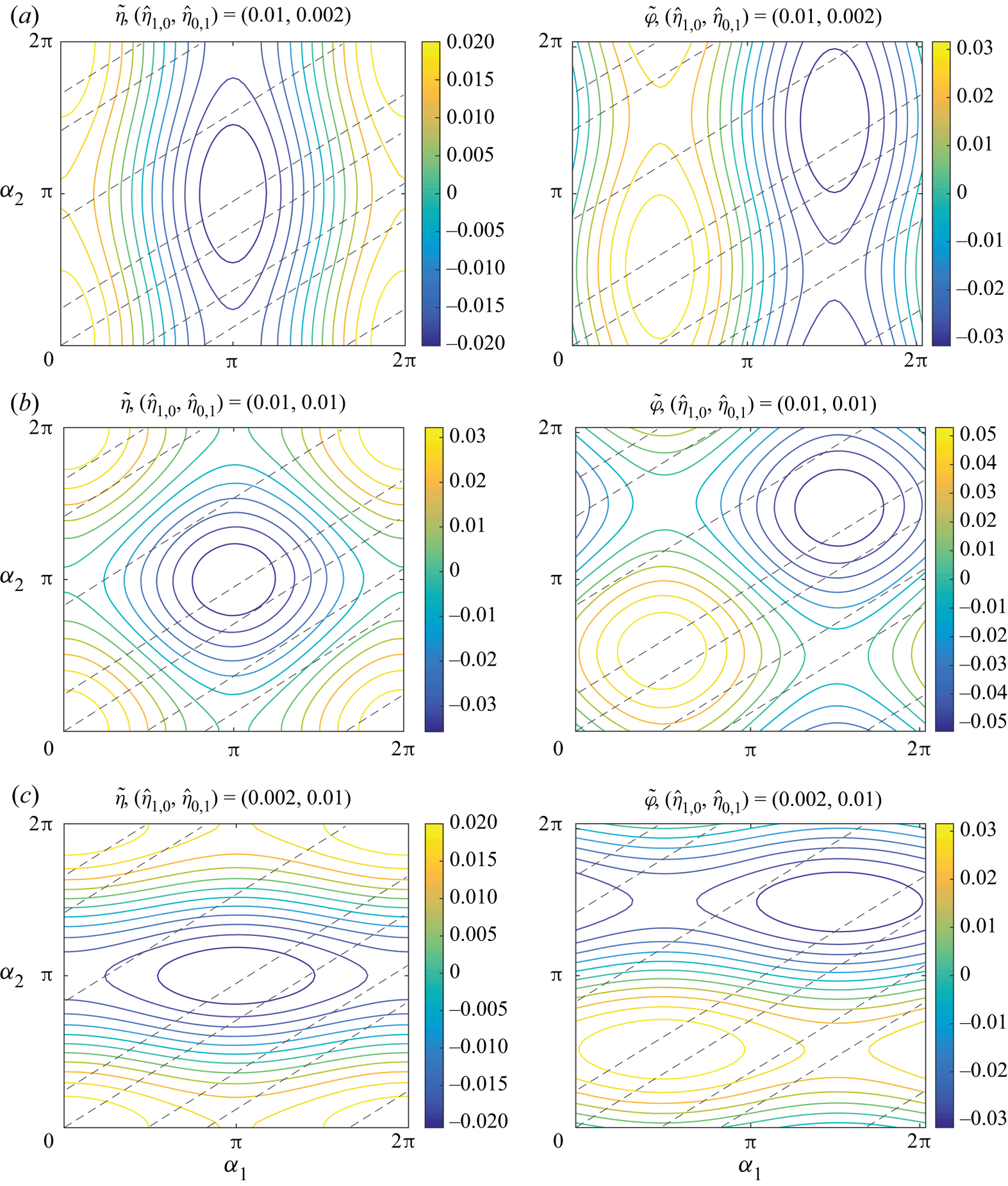
The amplitude ratio,  $\gamma := \hat {\eta }_{1,0} / \hat {\eta }_{0,1}$, determines the bulk shape of the solution. If
  $\gamma \gg 1$, the component wave with wavenumber 1 will be dominant; if
  $\gamma \ll 1$, the component wave with wavenumber
  $k=1/\sqrt 2$ will be dominant; and if
  $\gamma$ is close to 1, both waves together will be dominant over higher-frequency Fourier modes (at least in the regime we study here). This is demonstrated with
  $\gamma =5$,
  $1$ and
  $0.2$ in panels (a), (b) and (c) of figure 1. Panels (a,c) show a clear dominant mode with visible variations in the amplitude. The oscillations are faster in panel (a) than in (c) since
  $1>k\approx 0.707$. By contrast, in panel (b), there is no single dominant wavelength.
This can also be understood from the contour plots of figure 2. In case (a),  $\gamma \gg 1$ and the contour lines of
  $\tilde \eta$ and
  $\tilde \varphi$ are perturbations of sinusoidal waves depending only on
  $\alpha _1$. The unperturbed waves would have vertical contour lines. The
  $\alpha _2$-dependence of the perturbation causes local extrema to form at the crest and trough. As a result, the contour lines join to form closed curves that are elongated vertically since the dominant variation is in the
  $\alpha _1$ direction. Case (c) is similar, but the contour lines are elongated horizontally since the dominant variation is in the
  $\alpha _2$ direction. Following the dashed lines in figure 2, a cycle of
  $\alpha _1$ is completed before a cycle of
  $\alpha _2$ (since
  $k<1$). In case (a), a cycle of
  $\alpha _1$ traverses the dominant variation of
  $\tilde \eta$ and
  $\tilde \varphi$ on the torus, whereas in case (c), this is true of
  $\alpha _2$. So the waves in figure 1 appear to oscillate faster in case (a) than case (c). In the intermediate case (b) with
  $\gamma =1$, the contour lines of the crests and troughs are nearly circular, but not perfectly round. The amplitude of the waves in figure 1 are largest when the dashed lines in figure 2 pass near the extrema of
  $\tilde \eta$ and
  $\tilde \varphi$, and are smallest when the dashed lines pass near the zero level sets of
  $\tilde \eta$ and
  $\tilde \varphi$.
Next we examine the behaviour of the Fourier modes that make up these solutions. Figure 3 shows two-dimensional plots of the Fourier modes  $\hat \eta _{j_1,j_2}$ for the 3 cases above, with
  $\gamma \in \{5,1,0.2\}$ and
  $max\{\hat \eta _{1,0},\hat \eta _{0,1}\}= 0.01$. Only the prescribed modes and the modes that were optimized by the solver (see (3.10)) are plotted, which have indices in the range
  $0\le j_1\le N$ and
  $-N\le j_2\le N$, excluding
  $j_2\le 0$ when
  $j_1=0$. The other modes are determined by the symmetry of (2.39a,b) and by zero padding
  $\hat \eta _{j_1,j_2}=0$ if
  $N < j_1\le M/2$ or
 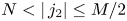 $N<|\,j_2|\le M/2$. We used
  $N=24$ and
  $M=60$ in all 3 calculations. One can see that the fixed Fourier modes
  $\hat {\eta }_{1,0}$ and
  $\hat {\eta }_{0,1}$ are the two highest-amplitude modes in all three cases. In this sense, our solutions of the nonlinear problem (2.37) are small-amplitude perturbations of the solutions (3.13) of the linearized problem. However, in the plots of figure 3, there are many active Fourier modes other than the four modes
  $\textrm {e}^{\pm \textrm {i}\alpha _1}$,
  $\textrm {e}^{\pm \textrm {i} \alpha _2}$ from linear theory. In this sense, these solutions have left the linear regime. Carrying out a weakly nonlinear Stokes expansion to high enough order to accurately predict all these modes would be difficult due to the two-dimensional array of unknown Fourier modes, which would complicate the analysis of the periodic Wilton ripple problem (Vanden-Broeck Reference Vanden-Broeck2010; Trichtchenko et al. Reference Trichtchenko, Deconinck and Wilkening2016; Akers et al. Reference Akers, Ambrose and Sulon2019; Akers & Nicholls Reference Akers and Nicholls2020). Steeper waves that are well outside of the linear regime will be computed in § 4.3.
Two-dimensional Fourier modes of  $\tilde \eta$ for the
  $k=1/\sqrt 2$ solutions plotted in figures 1 and 2: (a)
  $\gamma =5$; (b,d)
  $\gamma =1$; (c)
  $\gamma =0.2$. In all three cases, the modes decay visibly slower along the line
  $j_1+j_2k=0$, indicating the presence of resonant mode interactions.

In panels (a,b,c) of figure 3, the modes appear to decay more slowly in one direction than in other directions. This is seen more clearly when viewed from above, as shown in panel (d) for the case of  $\gamma =1$. (The other two cases are similar.) The direction along which the modes decay less rapidly appears to coincide with the line
 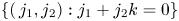 $\{(\,j_1,j_2):j_1+j_2k=0\}$, which is plotted in red. A partial explanation is that when
  $j_1+j_2k$ is close to zero, the corresponding modes
  $\textrm {e}^{\textrm {i}(\,j_1+j_2k)\alpha }$ in the expansion of
  $\eta (\alpha )$ in (2.12a,b) have very long wavelengths. Slowly varying perturbations lead to small changes in the residual of the water wave equations, so these modes are not strongly controlled by the governing equations (2.37). We believe this would lead to a small divisor problem that would complicate a rigorous proof of existence of quasi-periodic travelling water waves. Similar small divisor problems arise in proving the existence of standing water waves (Plotnikov & Toland Reference Plotnikov and Toland2001; Iooss et al. Reference Iooss, Plotnikov and Toland2005), three-dimensional travelling gravity waves (Iooss & Plotnikov Reference Iooss and Plotnikov2009) and two-dimensional time quasi-periodic gravity–capillary waves (Berti & Montalto Reference Berti and Montalto2016; Baldi et al. Reference Baldi, Berti, Haus and Montalto2018; Berti et al. Reference Berti, Franzoi and Maspero2020), where small divisors are tackled using a Nash–Moser iterative scheme.
Next we show that  $\tau$ and
  $c$ depend nonlinearly on the amplitude of the Fourier modes
  $\hat {\eta }_{1,0}$ and
  $\hat {\eta }_{0,1}$. Panels (a) and (b) of figure 4 show plots of
  $\tau$ and
  $c$ versus
 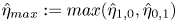 $\hat \eta _{max}:=max(\hat \eta _{1,0},\hat \eta _{0,1})$ for 9 values of
  $\gamma =\hat \eta _{1,0}/\hat \eta _{0,1}$, namely
  $\gamma =0.1, 0.2, 0.5, 0.8, 1, 1.25, 2, 5, 10$. On each curve,
  $\hat \eta _{max}$ varies from 0 to
  $0.01$ in increments of
  $0.001$. At small amplitude, linear theory predicts
 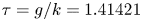 $\tau =g/k=1.41421$ and
 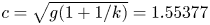 $c=\sqrt {g(1+1/k)}=1.55377$. This is represented by the black marker at
  $\hat \eta _{max}=0$ in each plot. For each value of
  $\gamma$, the curves
  $\tau$ and
  $c$ are seen to have zero slope at
  $\hat \eta _{max}=0$, and can be concave up or concave down depending on
  $\gamma$. This can be understood from the contour plots of panels (e,f). Both
  $\tau$ and
  $c$ appear to be even functions of
  $\hat \eta _{1,0}$ and
  $\hat \eta _{0,1}$ when the other is held constant. Both plots have a saddle point at the origin, are concave down in the
  $\hat \eta _{1,0}$ direction holding
  $\hat \eta _{0,1}$ fixed, and are concave up in the
  $\hat \eta _{0,1}$ direction holding
  $\hat \eta _{1,0}$ fixed. The solid lines in the first quadrant of these plots are the slices corresponding to the values of
  $\gamma$ plotted in panels (a,b). The concavity of the one-dimensional plots depends on how these lines intersect the saddle in the two-dimensional plots.
Surface tension, wave speed, energy and momentum of small-amplitude quasi-periodic water waves with  $k=1/\sqrt 2$. (a–d) Plots of
  $\tau$,
  $c$,
$c$,  $E$ and
  $P_x$ versus
  $\hat {\eta }_{max}=max\{\hat \eta _{1,0},\hat \eta _{0,1}\}$ holding
  $\gamma =\hat \eta _{1,0}/\hat \eta _{0,1}$ fixed. The black arrow in each plot shows how the curves change as
  $\gamma$ increases from
  $0.1$ to
  $10$. (e, f) Contour plots of
  $\tau$ and
  $c$ and the rays of constant
  $\gamma$ corresponding to (a,b). (g) Mode amplitudes of a two-dimensional Chebyshev expansion of
  $c(\hat \eta _{1,0},\hat \eta _{0,1})$ over the rectangle
  $-0.01\le \hat \eta _{1,0},\hat \eta _{0,1}\le 0.01$.

The contour plots of panels (e,f) of figure 4 were made by solving (2.37) with  $(\hat \eta _{1,0},\hat \eta _{0,1})$ ranging over a uniform
  $26\times 26$ grid on the square
  $[-0.01,0.01]\times [-0.01,0.01]$. Using an even number of grid points avoids the degenerate case where
  $\hat \eta _{1,0}$ or
  $\hat \eta _{0,1}$ is zero. At those values, the two-dimensional family of quasi-periodic solutions meets a sheet of periodic solutions where
  $\tau$ or
  $c$ becomes a free parameter. Alternative techniques would be needed in these degenerate cases to determine the value of
  $\tau$ or
  $c$ from which a periodic travelling wave in the nonlinear regime bifurcates to a quasi-periodic wave. In panel (g), we plot the magnitude of the Chebyshev coefficients in the expansion
 \begin{equation} c(\hat\eta_{1,0},\hat\eta_{0,1}) = \sum_{m=0}^{15}\sum_{n=0}^{15} \hat c_{mn}T_m(100\hat\eta_{1,0})T_n(100\hat\eta_{0,1}), \quad -0.01\le \hat\eta_{1,0},\hat\eta_{0,1}\le 0.01. \end{equation}
This was done by evaluating  $c$ on a cartesian product of two 16-point Chebyshev–Lobatto grids over
  $[-0.01,0.01]$ and using the one-dimensional fast Fourier transform in each direction to compute the Chebyshev modes. We see that the modes decay to machine precision by the time
  $m+n\ge 10$ or so, and only even modes
  $m$ and
  $n$ are active. The plot for
  $|\hat \tau _{mn}|$ is very similar, so we omit it. These plots confirm the visual observation from the contour plots that
  $\tau$ and
  $c$ are even functions of
  $\hat \eta _{1,0}$ and
  $\hat \eta _{0,1}$ when the other is held constant. These properties of
  $\tau$ and
  $c$ make them unsuitable as continuation parameters near the trivial solution, as discussed in § 3.
In panels (c,d) of figure 4, we show the energy  $E$ and momentum
  $P_x$ of waves in the above two-parameter family of quasi-periodic solutions,
 \begin{equation} \left. \begin{array}{c@{}} \begin{aligned} E & = \int_{\mathbb{T}^2} \tfrac{1}{2} \tilde{\psi}(\partial_{\alpha_1} + k\partial_{\alpha_2})\tilde{\varphi} + \tfrac{1}{2} g\tilde{\eta}^2(1+ (\partial_{\alpha_1} + k\partial_{\alpha_2})\tilde{\xi}) \\ & \quad + \tau\left(\sqrt{(1+ (\partial_{\alpha_1} + k\partial_{\alpha_2})\tilde{\xi})^2 + ((\partial_{\alpha_1} + k\partial_{\alpha_2})\tilde{\eta})^2} - 1\right)\, \textrm{d} \alpha_1\,\textrm{d} \alpha_2, \end{aligned}\\ P_x ={-}\displaystyle\int_{\mathbb{T}^2} \tilde{\varphi}(\partial_{\alpha_1} + k\partial_{\alpha_2})\tilde{\eta}\, \textrm{d} \alpha_1 \,\textrm{d} \alpha_2. \end{array}\right\} \end{equation}
These formulas are derived by Zakharov et al. (Reference Zakharov, Dyachenko and Vasilyev2002) and Dyachenko, Lushnikov & Zakharov (Reference Dyachenko, Lushnikov and Zakharov2019) in the conformal mapping framework for a water wave of infinite depth. The only modification needed for spatially quasi-periodic waves with  $d$ quasi-periods is that integrals over
  $\mathbb{R}$ or
  $\mathbb{T}$ are replaced by integrals over
  $\mathbb{T}^d$. Wilkening & Zhao (Reference Wilkening and Zhao2020) confirm that
  $E$ and
  $P_x$ in (4.3) are conserved quantities under the evolution equations (2.27). We see in figure 4 that the energy and momentum of the quasi-periodic waves are positively correlated. In particular, the quasi-periodic wave family with
  $\gamma = 1$ possesses the largest energy and momentum when
  $\hat {\eta }_{max}$ is fixed, even though it does not have the highest wave speed. Energy and momentum can both be regarded as measures of the amplitude of the wave. Unlike the wave speed, they are both zero at the flat rest state. We note that
  $\gamma =1$ corresponds to maximizing both
  $|\eta _{1,0}|$ and
  $|\eta _{0,1}|$ to have the value
  $\hat {\eta }_{max}$, and also leads to the largest-amplitude oscillations in figure 1. The Hamiltonian structure of the equations of motion could be useful e.g. in generalizing the time quasi-periodic results of Berti et al. (Reference Berti, Franzoi and Maspero2020) to the spatially quasi-periodic setting.
4.2. Time evolution of spatially quasi-periodic travelling waves
In this section, we confirm that the quasi-periodic solutions we obtain by minimizing the objective function (3.11) are indeed travelling waves under the evolution equations (2.27). This allows us to measure the accuracy of our independent codes for solving these two problems by comparing the numerical results. An interesting feature of the conformal mapping formulation arises in this comparison, namely that for most choices of  $C_1$ in (2.27), travelling waves move at a non-uniform speed through conformal space in order to travel at constant speed in physical space. This is discussed in this section and proved in Appendix A.
In figure 5, we plot the time evolution of  $\zeta (\alpha ,t)$ in the laboratory frame from
  $t=0$ to
  $t=3$. The initial conditions, plotted with thick blue lines, are those of the travelling waves computed in figures 1 and 2 above by minimizing the objective function (3.11). The grey curves give snapshots of the solution at uniformly sampled times with
  ${\rm \Delta} t=0.1$. They were computed using the fifth-order explicit Runge–Kutta method described by Wilkening & Zhao (Reference Wilkening and Zhao2020) with a step size of 1/300, so there are 30 Runge–Kutta steps between snapshots in the figure. The solutions are plotted over the representative interval
  $0\le x\le 12{\rm \pi}$, though they extend in both directions to
  $\pm \infty$ without exactly repeating. The initial condition and time evolution were computed on the torus and then sampled along the
  $(1,k)$ direction to extract the data for these one-dimensional plots.
Time evolution of the travelling wave profiles,  $\zeta (\alpha ,t)$, from
  $t=0$ to
  $t=3$ in the laboratory frame. The thick blue lines correspond to the initial conditions.

For quantitative comparison, let  $\tilde \eta _0(\boldsymbol \alpha )$ denote the initial condition on the torus, which is computed numerically by minimizing (3.11). We then compute
  $\tilde \xi _0=H[\tilde \eta _0]$ and
  $\tilde \varphi _0=c\tilde \xi _0$, which are odd functions of
  $\boldsymbol \alpha =(\alpha _1,\alpha _2)\in \mathbb{T}^2$ since
  $\tilde \eta$ is even. From Corollary A.5 of Appendix A, we define the ‘exact solution’ of the time evolution of the travelling wave under (2.27) and (2.28) with these initial conditions as
 \begin{equation} \left. \begin{gathered} \tilde\eta_{exact}(\boldsymbol\alpha,t) = \tilde\eta_0(\boldsymbol\alpha - \boldsymbol k \alpha_0(t)), \\ \tilde\varphi_{exact}(\boldsymbol\alpha,t) = \tilde\varphi_0(\boldsymbol\alpha - \boldsymbol k\alpha_0(t)), \end{gathered}\right\} \end{equation}
where  $\boldsymbol k=(1,k)$,
 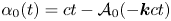 $\alpha _0(t)=ct - \mathcal{A}_0(-\boldsymbol kct)$ and
  $\mathcal{A}_0(x_1,x_2)$ is a periodic function on
  $\mathbb{T}^2$ defined implicitly by (A12) below. We see in (4.4) that the waves do not change shape as they move through the torus along the characteristic direction
  $\boldsymbol k$, but the travelling speed
  $\alpha _0'(t)$ in conformal space varies in time in order to maintain
  $\tilde \xi (0,0,t)=0$ via (2.28). By Corollary A.5, the exact reconstruction of
  $\tilde \xi _{exact}$ from
  $\tilde \eta _{exact}$ is
 \begin{equation} \tilde\xi_{exact}(\boldsymbol\alpha,t) = \tilde\xi_0(\boldsymbol\alpha - \boldsymbol k\alpha_0(t)) + \delta_0(t), \end{equation}
where  $\delta _0(t) = ct-\alpha _0(t) = \mathcal{A}_0(-\boldsymbol kct)$ measures the deviation in position from travelling at the constant speed
  $ct$ in conformal space. The defining property (A12) of
  $\mathcal{A}_0(x_1,x_2)$ ensures that
  $\tilde \xi _{exact}(0,0,t)=0$.
The significance of  $\mathcal{A}_0$ is that the inverse of the mapping
  $\boldsymbol x = \boldsymbol \alpha + \boldsymbol k\tilde \xi _0(\boldsymbol \alpha )$ on
  $\mathbb{T}^2$, assuming it is single valued, is
 \begin{equation} \boldsymbol \alpha = \boldsymbol x + \boldsymbol k\mathcal{A}_0(\boldsymbol x). \end{equation}
This result of Wilkening & Zhao (Reference Wilkening and Zhao2020) allows us to express quasi-periodic solutions of the initial value problem in conformal space as quasi-periodic functions in physical space. In the travelling case considered here, the exact solutions on the torus in physical space are  $\tilde \eta _0^{phys}(\boldsymbol x-\boldsymbol kct)$ and
  $\tilde \varphi _0^{phys}(\boldsymbol x-\boldsymbol kct)$, where e.g.
 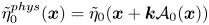 $\tilde \eta _0^{phys}(\boldsymbol x) = \tilde \eta _0(\boldsymbol x +\boldsymbol k \mathcal{A}_0(\boldsymbol x))$. We know this already on physical grounds, but it also follows from (4.4) and (4.5) using
 \begin{equation} \tilde\eta^{phys}_{exact}(\boldsymbol x,t) = \tilde\eta_{exact}(\boldsymbol x + \boldsymbol k\mathcal{A}(\boldsymbol x,t), t), \quad \tilde\varphi^{phys}_{exact}(\boldsymbol x,t) = \tilde\varphi_{exact}(\boldsymbol x + \boldsymbol k\mathcal{A}(\boldsymbol x,t), t), \end{equation}
where  $\mathcal{A}(\boldsymbol x,t) = \mathcal{A}_0(\boldsymbol x-\boldsymbol kct) - \mathcal{A}_0(-\boldsymbol kct)$ satisfies the time-dependent analogue of (A12).
Figure 6 shows contour plots of the torus version of the  $\gamma =5$ and
  $\gamma =0.2$ solutions shown in panels (a,c) of figure 5 at the final time computed,
  $T=3$. A similar plot of the
  $\gamma =1$ solution is given in Wilkening & Zhao (Reference Wilkening and Zhao2020). The dashed lines show the trajectory from
  $t=0$ to
  $t=T$ of the wave crest that begins at
  $(0,0)$ and continues along the path
  $\alpha _1=\alpha _0(t),$
  $\alpha _2=k\alpha _0(t)$ through the torus in (4.4). The following table gives the phase speed,
  $c$, surface tension,
  $\tau$, translational shift in conformal space at the final time computed,
  $\alpha _0(T)$, and deviation from steady motion in conformal space,
  $\delta _0(T)$, for these three finite-amplitude solutions (recall that
 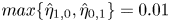 $max\{\hat \eta _{1,0},\hat \eta _{0,1}\}=0.01$ and
  $\hat \eta _{1,0}/\hat \eta _{0,1}=\gamma$) as well as for the zero-amplitude limit
 \begin{align}
\begin{array}{c|c|c|c|c} & \gamma=5 & \gamma=1 & \gamma =
0.2 & \text{linear theory} \\\hline c & \phantom{-} 1.552175 &
\phantom{-} 1.552197 & \phantom{-} 1.553743 & c_{lin} =
1.553774 \\ \tau & \phantom{-} 1.409665 & \phantom{-}
1.410902 & \phantom{-} 1.415342 & \tau_{lin} = 1.414214 \\
\alpha_0(T) & \phantom{-} 4.677416 & \phantom{-} 4.681174 &
\phantom{-} 4.668757 & c_{lin}T = 4.661322 \\
\delta_0(T) & -0.020890 & -0.024583 & -0.007527 & 0\end{array} \quad \begin{array}{c} \\ \\ \\ (T=3).
\end{array} \end{align}
\begin{align}
\begin{array}{c|c|c|c|c} & \gamma=5 & \gamma=1 & \gamma =
0.2 & \text{linear theory} \\\hline c & \phantom{-} 1.552175 &
\phantom{-} 1.552197 & \phantom{-} 1.553743 & c_{lin} =
1.553774 \\ \tau & \phantom{-} 1.409665 & \phantom{-}
1.410902 & \phantom{-} 1.415342 & \tau_{lin} = 1.414214 \\
\alpha_0(T) & \phantom{-} 4.677416 & \phantom{-} 4.681174 &
\phantom{-} 4.668757 & c_{lin}T = 4.661322 \\
\delta_0(T) & -0.020890 & -0.024583 & -0.007527 & 0\end{array} \quad \begin{array}{c} \\ \\ \\ (T=3).
\end{array} \end{align}
In figure 7, we plot  $\delta _0(t)$ for
  $0\le t\le T$ (solid lines) along with
  $(c-c_{lin})t$ (dashed and dotted lines) for the three finite-amplitude solutions in this table. Writing
  $\alpha _0(t) = c_{lin}t + [(c-c_{lin})t - \delta _0(t)]$, we see that the deviation of
  $\alpha _0(t)$ from linear theory over this time interval is due mostly to fluctuations in
  $\delta _0(t)$ rather than the steady drift
  $(c-c_{lin})t$ due to the change in phase speed
  $c$ of the finite-amplitude wave.
Contour plots of the numerical solution  $\tilde \eta (\alpha _1,\alpha _2,T)$ on the torus corresponding to the quasi-periodic solutions
  $\eta (\alpha ,t)$ of panels (a,c) of figure 5 at the final time shown,
  $t=T=3$. The dashed lines show the trajectory of the wave crest from
  $t=0$ to
  $t=T$.

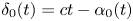


Computing the exact solution (4.4) requires evaluating  $\delta _0(t) = \mathcal{A}_0(-ct,-kct)$. We use Newton's method to solve the implicit equation (A12) for
  $\mathcal{A}_0(x_1,x_2)$ at each point of a uniform
  $M\times M$ grid, with
  $M_1=M_2=M$ in the notation of § 3. We then use FFTW to compute the two-dimensional Fourier representation of
  $\mathcal{A}_0(x_1,x_2)$, which is used to quickly evaluate the function at any point. It would also have been easy to compute
  $\mathcal{A}_0(-ct,-kct)$ directly by Newton's method, but the Fourier approach is also very fast and gives more information about the function
  $\mathcal{A}_0(x_1,x_2)$. In particular, the modes decay to machine roundoff on the grid, corroborating the assertion of Wilkening & Zhao (Reference Wilkening and Zhao2020) that
  $\mathcal{A}_0$ is real analytic. We use the exact solution to compute the error in time stepping (2.27) and (2.28) from
  $t=0$ to
  $t=T$,
 \begin{align} \text{err} = \sqrt{\|\tilde\eta-\tilde\eta_{{exact}}\|^2 + \|\tilde\varphi-\tilde\varphi_{{exact}}\|^2}, \quad \|\tilde\eta\|^2 = \frac1{M_1M_2}\sum_{m_1,m_2} \tilde\eta\left(\frac{2{\rm \pi} m_1}{M_1},\frac{2{\rm \pi} m_2}{M_2},T\right)^2. \end{align}
A detailed convergence study is given in Wilkening & Zhao (Reference Wilkening and Zhao2020) to compare the accuracy and efficiency of the Runge–Kutta and exponential time differencing schemes proposed in that paper using the  $\gamma =1$ travelling solution above as a test case. Here we report the errors for all three waves plotted in figure 5
 \begin{equation} \begin{array}{c|c|c|c} & \gamma=5 & \gamma=1 & \gamma=0.2 \\\hline \text{err} & 1.04\times10^{{-}16} & 1.16\times10^{{-}16} & 7.38\times10^{{-}17} \end{array}, \end{equation}
using the simplest time stepping method of Wilkening & Zhao (Reference Wilkening and Zhao2020) to solve (2.27), namely a fifth-order explicit Runge–Kutta method using 900 uniform steps from  $t=0$ to
  $t=3$. These errors appear to mostly be due to roundoff error in floating-point arithmetic, validating the accuracy of both the time stepping algorithm of Wilkening & Zhao (Reference Wilkening and Zhao2020) and the travelling wave solver of § 3, which was taken as the exact solution. Evolving the solutions to compute these errors took less than a second on a laptop (with
  $M^2=3600$ grid points and 900 time steps), while computing the travelling waves via the Levenberg-Marquardt method took 7 seconds on a laptop and only 0.9 seconds on a server (Intel Xeon Gold 6136, 3GHz) running on 12 threads (with
  $M^2=3600$ grid points and
  $N_{tot}=1200$ unknowns).
4.3. Larger-amplitude gravity–capillary waves
In the previous sections we studied the full two-parameter family of quasi-periodic travelling waves with  $k=1/\sqrt 2$, varying both
  $\hat \eta _{1,0}$ and
  $\hat \eta _{0,1}$ over the range
  $[-0.01,0.01]$. Here we search for larger-amplitude waves along the path
  $\gamma =1$, where
  $\hat \eta _{1,0}=\hat \eta _{0,1}=\hat \eta _{max}$ serves as an amplitude parameter. The calculations are done on an
  $M\times M$ grid with Fourier cutoff
  $N$. As the amplitude increases with
  $M$ and
  $N$ fixed, the Fourier modes outside of the cutoff region
  $max(|\,j_1|,|\,j_2|)\le N$ eventually grow in magnitude to exceed
  $\varepsilon \hat \eta _{max}$, where
  $\varepsilon$ is machine precision. Because we formulate the problem as an overdetermined least-squares problem, it ceases to be possible to satisfy all the equations with the limited number of Fourier degrees of freedom, and the minimum value of the objective function begins to grow rapidly with amplitude.
This is demonstrated in figure 8 using five grids ranging from  $(M,N)\,{=}\,(48,11)$ to
  $(M,N)=(240{,}100)$ and
  $\hat \eta _{max}$ ranging from
  $0.001$ to
  $0.029$. Because the objective function
  $f$ is a squared error, if the solution has 14 digits of accuracy the objective function will be around
  $10^{-28}$. The coarsest grid becomes under-resolved for
  $\hat \eta _{max}>0.013$ while the finest grid becomes under-resolved for
  $\hat \eta _{max}\ge 0.0281$. One can see from the two-dimensional Fourier plots in figure 3 that
  $N=24$ was overkill at the amplitude
  $\hat \eta _{max}=0.01$ since the modes have decayed below
  $\varepsilon \hat \eta _{max}=1.11\times 10^{-18}$ by the time
  $max(|\,j_1|,|\,j_2|)\ge 11$. But we see in figure 8 that once
  $\hat \eta _{max}$ reaches 0.021, it becomes necessary to increase
  $M$ and
  $N$ to maintain accuracy. At this amplitude, a two-dimensional Fourier plot (not shown) contains larger-amplitude modes extending all the way to the boundary of
  $max(|\,j_1|,|\,j_2|)\le 24$.
Minimum value of the objective function  $f$ for different values of
  $M$,
$M$,  $N$ and amplitude,
  $\hat \eta _{max}$. Each curve is labelled by two numbers,
  $M$ and
  $N$, with
  $N$ the smaller one. The objective function grows rapidly with
  $\hat \eta _{max}$ once there are not enough Fourier modes to represent the solution to machine precision.

The running time grows rapidly with grid size, with each calculation on the grids in figure 8 requiring an average of
 \begin{equation} \begin{array}{r|c|c|c|c|c} (M,N) & (48,11) & (72,24) & (96,40) & (192,75) & (240,100) \\\hline \text{running time} & 0.1\ \text{s} & 0.9\ \text{s} & 10.2\ \text{s} & 8.5\ \text{min} & 55.3\ \text{min} \end{array}, \end{equation}
on a 3 GHz server with 24 cores. The memory requirements also grow rapidly as several matrices of size  $M^2\times N_{tot}$ are computed in the Levenberg–Marquardt algorithm, namely the Jacobian and its (reduced) singular value decomposition. In the
  $(M,N)=(240,100)$ case, each of these matrices requires 9.3 GB of storage, and we are not able to increase the problem size further due to hardware limitations. As a possible future research direction, one can try to improve the performance of the Levenberg–Marquardt method for high-dimensional problems using Krylov subspace approximations (Lin, O'Malley & Vesselinov Reference Lin, O'Malley and Vesselinov2016) without computing the entire Jacobian or its singular value decomposition (SVD).
In figure 9(a), we plot the largest-amplitude ‘fully resolved’ solution in figure 8 with  $(M,N)=(240,100)$ and
  $(\hat {\eta }_{1, 0}, \hat {\eta }_{0, 1}) = (0.028, 0.028)$. The solid black curve is the nonlinear travelling wave, which has a maximum slope of
  $0.107$ over the representative interval
  $[0,10{\rm \pi} ]$ shown in the plot, while the dashed red curve is the linear prediction
  $\eta (\alpha ) = 0.056\cos (\alpha ) + 0.056\cos (\alpha /\sqrt {2})$. At this amplitude, there is a visible difference between the nonlinear and linear quasi-periodic waves, especially near the peaks and troughs of the waves. However, the difference is not large since the two base modes are still the dominant Fourier modes: the amplitudes of the other Fourier modes are less than 0.0035, which is
  $1/8$ of the base modes.
Plots of higher-amplitude quasi-periodic travelling waves. Panels (a,c) show the initial conditions  $\eta$ over
  $[0,10{\rm \pi} ]$. Panels (b,d) show the amplitudes of Fourier modes along different directions versus the magnitude of the two-dimensional mode index
  $(\,j_1,j_2)$.

One of the main obstacles to computing high-amplitude solutions numerically is the slow decay of Fourier modes along certain resonant directions. To demonstrate this, we plot in figure 9(b) the amplitudes of the Fourier modes of  $\tilde {\eta }$ along 7 directions:
  $j_1+akj_2\approx 0$ with
  $a\in \{1,1.1,0.9,1.5,0.5,0\}$ and
  $j_2 = 0$. Since
  $k$ is irrational, in direction
  $j_1 + akj_2 \approx 0$ we choose
  $j_1$ to be
  $min\{{floor}(-akj_2), N\}$ with
  $j_2\in \{-1,\ldots ,-N\}$. As shown in the figure, the Fourier modes decay more slowly when the ratio
  $-j_1/j_2$ is close to
  $k$. Even though
  $j_1 + k j_2 = 0$ is the resonant condition for linear quasi-periodic waves, the effects of this resonance persist into the nonlinear regime. Along the direction
  $j_1+kj_2\approx 0$, the mode with
  $(\,j_1,j_2)$ farthest from the origin is
  $\hat {\eta }_{70, -100}$ and its amplitude is
  $8.3\times 10^{-12}$, which is the point where floating-point error and finite
  $N$ truncation effects are roughly equal in this large-scale optimization problem.
In non-resonant directions, the modes decay faster, often remaining smaller than  $\varepsilon \hat \eta _{max}$. For example, curves (4)–(7) in figure 9(b) drop below
  $10^{-20}$ for
  $(\,j_1^2+j_2^2)\ge 50$, whereas
  $\varepsilon \hat \eta _{max}=(2^{-53})(0.028)=3.1\times 10^{-18}$. This may also be observed in the two-dimensional Fourier plots of figure 3. Presumably the columns
  $\partial \mathcal{R}/\partial p_j$ of the Jacobian corresponding to these modes remain nearly orthogonal to the residual
  $\mathcal{R}$ throughout the computation, so the Levenberg–Marquardt algorithm brings them into the calculation with very small coefficients. Since increasing the amplitude beyond
  $\hat \eta _{max}=0.028$ leads to loss of spectral accuracy, this is the largest-amplitude wave of this type that we can compute.
Next we look for steeper waves by modifying the surface tension parameter  $\tau$ and wavenumber ratio
  $k$. So far we have only shown calculations with
  $k = 1/\sqrt {2}$, which was an arbitrary choice. In ocean waves, the characteristic wavelength of gravity waves is larger than that of capillary waves by several orders of magnitude. Here we increase
  $k$ modestly to
 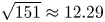 $\sqrt {151} \approx 12.29$, which is still much smaller than occurs in the ocean but could be relevant to a laboratory experiment. The case of pure gravity waves, which is more relevant to the ocean, will be undertaken in future work. Some comments on this were given in the introduction.
Rather than explore the two-parameter family of quasi-periodic water waves with  $k=\sqrt {151}$ near the trivial solution or follow a path holding
  $\gamma =\hat \eta _{1,0}/\hat \eta _{0,1}$ constant, we attempt to compute steep quasi-periodic travelling waves as small quasi-periodic perturbations of large-amplitude periodic waves, which are comparatively inexpensive to compute (Dyachenko et al. Reference Dyachenko, Lushnikov and Korotkevich2016; Trichtchenko et al. Reference Trichtchenko, Deconinck and Wilkening2016). In panel (e) of figure 4 above, the contour plot of
  $\tau (\hat \eta _{1,0},\hat \eta _{0,1})$ represents a surface in three-dimensional
  $(\hat \eta _{1,0},\hat \eta _{0,1},\tau )$ space. The coordinate planes
  $\hat \eta _{0,1}=0$ and
  $\hat \eta _{1,0}=0$ in this space are two additional surfaces representing travelling waves, the first of periodic waves of wavelength
  $2{\rm \pi}$ and the second of periodic waves of wavelength
  $2{\rm \pi} /k$. The two parameters on the
  $\hat \eta _{0,1}=0$ surface are
  $\tau$ and
  $\hat \eta _{1,0}$. This surface intersects the
  $\tau (\hat \eta _{1,0},\hat \eta _{0,1})$ surface along a curve
  $\tau (\hat \eta _{1,0},0)$ where it is possible to bifurcate from periodic travelling waves to quasi-periodic travelling waves. As explained after (4.2) above,
  $\tau (\hat \eta _{1,0},0)$ is an even function of
  $\hat \eta _{1,0}$, so its deviation from
  $\tau _{lin}$ is a second-order correction.
In the present case of  $k=\sqrt {151}$, we hold the surface tension fixed at
 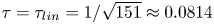 $\tau =\tau _{lin}=1/\sqrt {151} \approx 0.0814$ and use the Levenberg–Marquardt method to compute the resulting one-parameter family of
  $2{\rm \pi}$-periodic travelling waves, denoted as
  $\eta _{per}$, over the range
  $0\le \hat \eta _{1,0} \le 0.1$. At the amplitude
  $\hat \eta _{1,0}=0.1$, the Fourier modes
  $\hat \eta _{j_1}$ of
  $\eta _{per}(\alpha )$ decay to machine precision around
  $j_1=200$. The maximum slope of this wave in physical space is 0.332, which is about 3 times steeper than the quasi-periodic wave computed above with
  $k=1/\sqrt 2$ and
  $\hat \eta _{1,0}=\hat \eta _{0,1}=0.028$. Rather than search within the family of periodic waves for the bifurcation point
  $\tau (0.1,0)$, we attempt to jump directly onto the family of quasi-periodic waves from the periodic wave with
  $\tau =\tau _{lin}$. As an initial guess for the Levenberg–Marquardt method, we set
 \begin{equation} \tilde\eta^{(0)}(\alpha_1,\alpha_2) = \eta_{per}(\alpha_1) + \hat\eta_{0,1}( \textrm{e}^{\textrm{i}\alpha_2} + \textrm{e}^{-\textrm{i}\alpha_2}), \quad \tau^{(0)}=\tau_{lin}, \quad b^{(0)} = c_{per}^2, \end{equation}
in (4.1a–c), where  $c_{per}$ is the wave speed of
  $\eta _{per}$. We succeeded in minimizing the objective function to
  $f=8.4\times 10^{-29}$ holding
  $(\hat \eta _{1,0},\hat \eta _{0,1})$ fixed at
  $(0.1,0.00003)$ and using
  $(N_1,N_2)=(216,8)$ for the Fourier cutoffs on an
  $M_1\times M_2=576\times 24$ grid. Using smaller values
  $N_2 < N_1$ and
  $M_2 < M_1$ is possible since the unperturbed wave is independent of
  $\alpha _2$, and is required to make the problem computationally tractable. We then use numerical continuation to increase
  $\hat \eta _{0,1}$ to
  $0.0003$ in increments of
  $0.00003$, holding
  $\hat \eta _{1,0}=0.1$ fixed. Polynomial interpolation of
  $\tau (0.1,\hat \eta _{0,1})$ from the points
  $\hat \eta _{0,1}\in \{\pm 0.00003m: 1\le m\le 5\}$ gives the value
  $\tau (0.1,0)=0.0807311$ for the surface tension of the periodic travelling wave where the bifurcation to quasi-periodicity occurs. This is only
  $0.8\,\%$ smaller than
  $\tau _{lin}$, which explains why it was possible to find nearby quasi-periodic waves to the
  $\tau =\tau _{lin}$ periodic waves even though this is not the precise location of the bifurcation.
The last solution on this path, with ( $\hat \eta _{1,0},\hat \eta _{0,1})=(0.1,0.0003)$, is shown in panels (c) and (d) of figure 9. We had to increase the Fourier cutoffs
  $(N_1,N_2)$ to
  $(350,30)$ and the grid to
  $M_1\times M_2 = 720\times 64$ to achieve spectral accuracy. The objective function for this quasi-periodic solution has been minimized to
  $f=1.8\times 10^{-25}$ and the maximum slope over the representative interval
  $[0,10{\rm \pi} ]$ is
  $0.448$, so this wave is 35 % steeper than
  $\eta _{per}$ and 4.2 times steeper than the
  $k=1/\sqrt 2$ wave of panels (a,b) of the figure. Hardware limitations prevented increasing
  $\hat \eta _{0,1}$ further since there are already
  $M_1M_2=46\,080$ nonlinear equations in
  $N_{tot}=21{\kern1pt}380$ unknowns. The wave speed and surface tension of this quasi-periodic wave are
  $\tau =0.0809677$ and
  $c=1.072419$, which are close to the values
  $\tau (0.1,0)=0.0807311$ and
  $c(0.1,0)=1.071972$ of the periodic wave at the bifurcation.
Panel (c) shows the nonlinear periodic and quasi-periodic travelling waves as well as the linear quasi-periodic travelling wave  $\eta = 0.2 \cos (\alpha ) + 0.0006 \cos (k\alpha )$ over the representative interval
  $[0,10{\rm \pi} ]$. Both nonlinear waves deviate from the linear wave by more than 50 % of the amplitude of the linear wave, which shows that these solutions are well outside of the linear regime. The difference between the periodic wave and the quasi-periodic wave is also visible, with the wave peak at
  $\xi =0$ perturbed upward and the others perturbed upward or downward and left or right, asymmetrically, in a non-repeating pattern. The small oscillations in the trough also change aperiodically from one trough to the next, which shows that some of the modes
  $\hat \eta _{j_1,j_2}$ with
  $j_2\ne 0$ are comparable in size to the modes of the periodic wave responsible for the capillary ripples in the troughs.
Panel (d) shows the Fourier mode amplitudes  $\hat \eta _{j_1,j_2}$ along various directions in the
  $(\,j_1,j_2)$ lattice. Along the direction
  $j_1 + akj_2 \approx 0$ we choose
  $j_1$ to be
  $min\{\,{floor}(-akj_2), N_1\}$ with
  $j_2\in \{-1,\ldots ,-N_2\}$. One can see that the Fourier modes decay more slowly along directions
  $j_1 + akj_2 \approx 0$ when
  $a\in \{1,1.1,0.9,1.5\}$ than when
  $a\in \{0.5,0\}$ or when
  ${j_2\approx 0}$. Thus, the linear resonance condition
  $j_1 + k j_2 = 0$ continues to have a large effect on the Fourier modes in the nonlinear regime. As noted in § 4.1 above, we believe this is because the corresponding modes
  $\textrm {e}^{\textrm {i}(\,j_1+j_2k)\alpha }$ in the expansion of
  $\eta (\alpha )$ in (2.12a,b) have long wavelengths and are not as strongly controlled by the governing equations (2.37) as other modes, which leads to greater sensitivity to nonlinear interactions among the Fourier modes.
5. Conclusion
In this work, we have formulated the two-dimensional, infinite depth gravity–capillary travelling wave problem in a spatially quasi-periodic, conformal mapping framework. We have numerically demonstrated the existence of travelling solutions that are a quasi-periodic generalizations of Wilton's ripples. To compute them, we adapted an overdetermined nonlinear least-squares technique introduced by Wilkening & Yu (Reference Wilkening and Yu2012) for a different problem. For each solution computed, the value of  $k$ and the amplitudes of two base Fourier modes
  $\hat {\eta }_{1,0}$ and
  $\hat {\eta }_{0,1}$ are fixed while
  $\tau$,
  $c$ and the other Fourier modes
  $\hat \eta _{j_1,j_2}$ are varied to search for solutions of (2.37). Before minimizing (3.11), the initial guess for each solution is computed using either the linear approximation (3.13) or numerical continuation. We obtained quasi-periodic travelling solutions with maximum slope as large as 0.448 and validated the accuracy of the travelling solutions using the time stepping algorithm of Wilkening & Zhao (Reference Wilkening and Zhao2020). To evolve at constant speed in physical space, we have shown that the two-dimensional representation of the quasi-periodic waves travel at a non-uniform speed through the torus. We explain this by constructing a change of variables, namely (4.6), relating quasi-periodic functions in conformal space to quasi-periodic functions in physical space with the same wavenumber ratio
  $k$.
$k$.
As the amplitude increases, we have found that the wave spectrum of a quasi-periodic travelling wave continues to decay exponentially, but becomes much broader than in the linear and weakly nonlinear approximations. For example, the solution shown in panels (c,d) of figure 9 has 23 modes within  $1\,\%$ of
  $\hat \eta _{1,0}$, 265 within a factor of
  $10^{-5}$, 1500 within a factor of
  $10^{-9}$ and 21 380 involved in the calculation. We also demonstrated the nonlinear dependence of wave speed, surface tension, energy and momentum for the two-parameter family with amplitude parameters in the range
  $max\{|\hat \eta _{1,0}| , |\hat \eta _{0,1}|\}\le 0.01$. Resonance effects were always observed in the Fourier modes
  $\hat \eta _{j_1,j_2}$ near the line
  ${j_1+j_2k=0}$, which is the resonance condition for linear waves. We provided the explanation that these modes are slowly varying when evaluated along the characteristic direction
  $(1,k)$ in the torus, and therefore are not strongly controlled by the Euler equations even for large-amplitude waves in the nonlinear regime. Additional resonance effects could be investigated in the future using Fourier–Bloch stability techniques (Longuet-Higgins Reference Longuet-Higgins1978; Deconinck & Oliveras Reference Deconinck and Oliveras2011; Trichtchenko et al. Reference Trichtchenko, Deconinck and Wilkening2016) generalized to the case of large-amplitude quasi-periodic travelling waves.
The question of what happens in our framework if  $k$ is rational is interesting. We believe the initial value problem (2.27) could still be solved, though in that case solving the torus version of the equations is equivalent to simultaneously computing a family of one-dimensional solutions on a periodic domain. Families of one-dimensional waves corresponding to a single solution of the torus problem are discussed in detail by Wilkening & Zhao (Reference Wilkening and Zhao2020), and take the form (2.30) above. If
  $k=q/p$ with
  $p$ and
  $q$ relatively prime integers, the waves in this family all have period
  $2{\rm \pi} p$. The travelling wave problem becomes degenerate if
  $k$ is rational – solutions of the torus version of (2.37) may still exist (we do not know), but if so, they are not unique. Indeed, if
  $k=q/p$ as above and
  $\tilde \eta _1$ solves the torus version of (2.37), then for any
  $2{\rm \pi}$-periodic, real analytic function
  $\alpha _0(r)$,
 \begin{equation} \tilde\eta_2\begin{pmatrix} \alpha_1\\ \alpha_2\end{pmatrix} = \tilde\eta_1\left(\begin{pmatrix} \alpha_1\\ \alpha_2\end{pmatrix} - \begin{pmatrix} p \\ q \end{pmatrix} \alpha_0 ({-}q\alpha_1 + p\alpha_2 )\right), \end{equation}
will also be a solution of (2.37) since the corresponding one-dimensional functions passing through the torus along characteristic lines are related by a simple reparameterization,
 \begin{equation} \eta_2(\alpha;\theta) = \tilde\eta_2\begin{pmatrix} \alpha \\ \theta + k\alpha \end{pmatrix} = \tilde\eta_1\begin{pmatrix} \alpha-p\alpha_0(p\theta) \\ \theta + k\alpha - q\alpha_0(p\theta) \end{pmatrix} = \eta_1(\alpha-p\alpha_0(p\theta);\theta). \end{equation}
Another degeneracy is that the modes  $\hat \eta _{j_1,j_2}$ of a solution of (2.37) with
  $j_1+kj_2=0$ and
  $(\,j_1,j_2)\ne\,(0,0)$ can be modified arbitrarily (maintaining
  $\hat \eta _{-j_1,-j_2}=\overline {\hat \eta _{j_1,j_2}}$) to obtain additional solutions of (2.37). These modes are plane waves that only affect the one-dimensional functions passing through the torus along characteristic lines by an additive constant. The resonance phenomenon observed in the Fourier modes in figure 3 is presumably a small divisor phenomenon (Iooss & Plotnikov Reference Iooss and Plotnikov2009) in the irrational case related to this degeneracy. If solutions for rational
  $k$ exist, a natural open question is whether they can be selected to fit together continuously with solutions for nearby irrational wavenumbers. In floating-point arithmetic, irrational wavenumbers are approximated by rational ones. We did not encounter difficulties with this, presumably because the above degeneracies are not visible with the grid resolution used. More work is needed to understand this rigorously.
The amplitude ratio  $\gamma =\hat \eta _{1,0}/\hat \eta _{0,1}$ plays an important role in determining the shapes of smaller-amplitude solutions. As seen in figures 1 and 5, the quasi-periodic features of the solutions are most evident when
  $\gamma \approx 1$. For larger-amplitude waves such as the one plotted in figure 9(c), quasi-periodicity can lead to visible changes from one peak or trough to the next, without ever repeating. It is remarkable that such a complicated aperiodic wave train is a stationary solution of the Euler equations in a moving frame.
In the future, we hope to explore the long-time dynamics of unstable subharmonic perturbations of periodic waves; to search for quasi-periodic travelling waves that bifurcate from large-amplitude periodic gravity waves or from overhanging gravity–capillary waves; to study the behaviour of different perturbation families, e.g. fixing the amplitudes of different base Fourier modes in (2.42) such as  $\hat {\eta }_{1,0}$ and
  $\hat {\eta }_{1,1}$; to study the stability of co-propagating quasi-periodic travelling waves and compare to the effects of oblique multi-phase interacting wave trains (Onorato et al. Reference Onorato, Osborne and Serio2006; Ablowitz & Horikis Reference Ablowitz and Horikis2015); to develop a generalization of Fourier–Bloch stability analysis for quasi-periodic waves, which presumably will further increase the number of quasi-periods of the perturbed wave; and to study finite-depth effects on both the initial value problem and the travelling wave problem. Additional future research challenges include establishing rigorous existence proofs; improving the algorithm to employ a Newton–Krylov or limited-memory approach so that it is not necessary to compute or factor the entire Jacobian matrix; and developing a formulation for quasi-periodic three-dimensional water waves, which would require abandoning the conformal mapping framework.
Funding
This work was supported in part by the National Science Foundation under award number DMS-1716560 and by the Department of Energy, Office of Science, Applied Scientific Computing Research, under award number DE-AC02-05CH11231.
Declaration of interest
The authors report no conflict of interest.
Appendix A. Dynamics of travelling waves in conformal space
In this section we study the dynamics of the travelling waves of § 2.4 under the evolution equations (2.27) for various choices of  $C_1$. We show that the waves maintain a permanent form but generally travel at a non-uniform speed in conformal space. We start by showing that there is a choice of
  $C_1$ for which
  $\eta$ and
  $\varphi$ remain stationary in time. We then show how
  $C_1$ changes when the waves are phase shifted by
  $\alpha _0(t)$, and how to determine
  $\alpha _0(t)$ so that
  $C_1$ takes the value in (2.28). The evolution of the torus version of (2.37) under (2.27) is also worked out.
We will need the following theorem and corollary, proved in Wilkening & Zhao (Reference Wilkening and Zhao2020):
Theorem A.1 Suppose  $\varepsilon >0$ and
  $z(w)$ is analytic on the half-plane
  $\mathbb{C}^-_\varepsilon = \{w: \operatorname {Im} w<\varepsilon \}$. Suppose there is a constant
  $M>0$ such that
  $|z(w)-w|\le M$ for
  $w\in \mathbb{C}^-_\varepsilon$, and that the restriction
  $\zeta =z\vert _\mathbb{R}$ is injective. Then the curve
  $\zeta (\alpha )$ separates the complex plane into two regions, and
  $z(w)$ is an analytic isomorphism of the lower half-plane onto the region below the curve
  $\zeta (\alpha )$.
Corollary A.2 Suppose  $k>0$ is irrational,
  $\tilde \eta (\alpha _1,\alpha _2)=\sum _{(\,j_1,j_2)\in \mathbb{Z}^2} \hat \eta _{j_1,j_2}\,\textrm {e}^{\textrm {i}(\,j_1\alpha _1+j_2\alpha _2)}$, and there exist constants
  $C$ and
  $\varepsilon >0$ such that
 \begin{equation} \hat\eta_{{-}j_1,-j_2}=\overline{\hat\eta_{j_1,j_2}}, \quad |\hat\eta_{j_1,j_2}|\le C\, \textrm{e}^{{-}3\varepsilon Kmax(|\,j_1|,|\,j_2|)}, \quad (\,j_1,j_2)\in\mathbb{Z}^2, \end{equation}
where  $K=max(k,1)$. Let
  $x_0$ be real and define
  $\tilde \xi =x_0+H[\tilde \eta ]$,
  $\tilde \zeta = \tilde \xi +i\tilde \eta$ and
 \begin{equation} \tilde z(\alpha_1,\alpha_2,\beta) = x_0 + i\hat\eta_{0,0} + \sum_{j_1+j_2k<0} 2i\hat\eta_{j_1,j_2}\, \textrm{e}^{-(\,j_1+j_2k)\beta}\,\textrm{e}^{\textrm{i}(\,j_1\alpha_1+ j_2\alpha_2)}, \quad (\beta<\varepsilon), \end{equation}
where the sum is over all integer pairs  $(\,j_1,j_2)$ satisfying the inequality. Suppose also that for each fixed
  $\theta \in [0,2{\rm \pi} )$, the function
  $\alpha \mapsto \zeta (\alpha;\theta )= \alpha +\tilde \zeta (\alpha ,\theta +k\alpha )$ is injective from
  $\mathbb{R}$ to
  $\mathbb{C}$ and
  $\zeta _\alpha (\alpha;\theta )\ne 0$ for
  $\alpha \in \mathbb{R}$. Then, for each
  $\theta \in \mathbb{R}$, the curve
  $\zeta (\alpha;\theta )$ separates the complex plane into two regions and
 \begin{equation} z(\alpha+i\beta;\theta) = (\alpha+i\beta) + \tilde z(\alpha,\theta+k\alpha,\beta), \quad (\beta<\varepsilon), \end{equation}
is an analytic isomorphism of the lower half-plane onto the region below  $\zeta (\alpha;\theta )$. Moreover, there is a constant
  $\delta >0$ such that
  $|z_w(w;\theta )|\ge \delta$ for
  $\operatorname {Im} w\le 0$ and
  $\theta \in \mathbb{R}$.
We now prove a theorem and two corollaries that describe the dynamics of travelling waves in conformal space under the evolution equations (2.27) for various choices of  $C_1$.
Theorem A.3 Suppose  $\tilde \eta _0(\alpha _1,\alpha _2)$ satisfies the torus version of (2.37) as well as the assumptions in Corollary A.2. Define
  $\tilde \xi _0 = H[\tilde \eta _0]$,
  $\tilde \zeta _0=\tilde \xi _0+i\tilde \eta _0$ and
  $\tilde \varphi _0=c\tilde \xi _0$. Let
  $\eta _0(\alpha;\theta )=\tilde \eta _0(\alpha ,\theta +k\alpha )$,
  $\varphi _0(\alpha;\theta )=\tilde \varphi _0(\alpha ,\theta +k\alpha )$,
  $\xi _0(\alpha;\theta )=\alpha +\tilde \xi _0(\alpha ,\theta +k\alpha )$ and
  $\zeta _0=\xi _0+i\eta _0$. Suppose that for each
  $\theta \in [0,2{\rm \pi} )$,
  $\alpha \mapsto \zeta _0(\alpha;\theta )$ is injective, i.e. none of the curves in the family (2.40) self-intersect. Then for each
  $\theta \in \mathbb{R}$,
 \begin{equation} \zeta(\alpha,t;\theta) = \zeta_0(\alpha;\theta)+ct, \quad \varphi(\alpha,t;\theta) = \varphi_0(\alpha;\theta), \end{equation}
satisfy (2.27) with  $C_1=cP_0[\xi _\alpha /J]$.
Proof. We have assumed the initial reconstruction of  $\xi$ from
  $\eta$ yields
  $\xi (\alpha ,0;\theta )=\xi _0(\alpha;\theta )$, so
  $x_0(0)=0$ in (2.13a,b). We need to show that
  $\eta _t=0$,
  $\varphi _t=0$ and
  $\textrm{d}\kern0.7pt x_0/ \textrm {d} t=c$ in (2.27), from which it follows that
  $\xi (\alpha ,t;\theta )=\xi _0(\alpha;\theta )+ct$. Since
  $\tilde \xi _0=H[\tilde \eta _0]$ and none of the curves in the family (2.40) self-intersect, Theorem A.1 and Corollary A.2 above show that the holomorphic extension from
  $\zeta _0(\alpha;\theta )$ to
  $z_0(w;\theta )$ is an analytic isomorphism of the lower half-plane to the fluid region, and
  $1/|z_{0,w}|$ is uniformly bounded. In (2.27), we define
  $\xi _\alpha =1+H[\eta _\alpha ]$,
  $\psi =-H[\varphi ]$,
  $J=\xi _\alpha ^2+\eta _\alpha ^2$ and
  $\chi =\psi _\alpha /J$. This formula for
  $\xi _\alpha$ gives the same result as differentiating
  $\xi (\alpha ,t;\theta )$ in (A4) with respect to
  $\alpha$. From
  $\tilde \varphi _0=c\tilde \xi _0$ and
  $\hat \eta _{0,0}=0$, we have
  $\chi =c\eta _\alpha /J$. The extension of
  $\zeta (\alpha ,t;\theta )$ to the lower half-plane is
  $z(w,t;\theta )=[z_0(w;\theta )+ct]$. We have not yet established that
  $\zeta (\alpha ,t;\theta )$ solves (2.27), but we know
  $z_t/z_w$ is bounded in the lower half-plane, so there is a
  $C_1$ such that
 \begin{equation} \begin{pmatrix} -H\chi + C_1 \\ -\chi \end{pmatrix} = \frac1J\begin{pmatrix} \xi_\alpha & \eta_\alpha \\ -\eta_\alpha & \xi_\alpha \end{pmatrix}\begin{pmatrix} c \\ 0 \end{pmatrix}, \end{equation}
where the right-hand side represents complex division of  $z_t$ by
  $z_\alpha$. Since
  $P_0H\chi =0$, we learn from (A5) that
  $C_1=cP_0[\xi _\alpha /J]$. But
  $\xi _t$ and
  $\eta _t$ in (2.25) are obtained by multiplying (A5) by
  $[\xi _\alpha ,-\eta _\alpha;\eta _\alpha , \xi _\alpha ]$, which gives
  $\xi _t=c$,
  $\eta _t=0$. Equation (2.26) is then
  $\textrm{d}\kern0.7pt x_0/ \textrm {d} t=P_0[\xi _t]=c$. Finally, using
  $\chi =c\eta _\alpha /J$,
  $H\chi = C_1-c\xi _\alpha /J$,
  $\varphi _\alpha =c(\xi _\alpha -1)$ and
  $\psi _\alpha =c\eta _\alpha$ in (2.27) gives
 \begin{align} \varphi_t &= P\left[\frac{\psi_\alpha^2 - \varphi_\alpha^2}{2J} - \varphi_\alpha H[\chi] + C_1\varphi_\alpha - g\eta + \tau\kappa\right] \nonumber\\ &= P\left[\frac{c^2\eta_\alpha^2 - c^2(\xi_\alpha^2-2\xi_\alpha+1)}{2J} + c\frac{c(\xi_\alpha-1)\xi_\alpha}{J} - g\eta + \tau\kappa\right] \nonumber\\ &= P\left[\frac{c^2}{2J}(J-1) - g\eta + \tau\kappa\right] = P\left[ -\frac{c^2}{2J}-g\eta + \tau\kappa\right] = 0, \end{align}
where we used (2.37) in the last step.
Corollary A.4 Suppose  $\tilde \zeta _0(\alpha _1,\alpha _2)$,
  $\tilde \varphi _0(\alpha _1,\alpha _2)$,
  $\zeta _0(\alpha;\theta )$ and
  $\varphi _0(\alpha;\theta )$ satisfy the hypotheses of Theorem A.3 and
  $\alpha _0(t)$ is any continuously differentiable, real-valued function. Then
 \begin{equation} \zeta(\alpha,t;\theta) = \zeta_0(\alpha-\alpha_0(t);\theta) +ct, \quad \varphi(\alpha,t; \theta) = \varphi_0(\alpha-\alpha_0(t);\theta), \end{equation}
are solutions of (2.27) with  $C_1=cP_0[\xi _\alpha /J]-\alpha _0'(t)$. The corresponding solutions of the torus version of (2.27) for this choice of
  $C_1$ are
 \begin{equation} \left. \begin{array}{c} \tilde\zeta(\alpha_1,\alpha_2,t) = \tilde\zeta_0(\alpha_1-\alpha_0(t), \alpha_2-k\alpha_0(t)) + ct - \alpha_0(t), \\ \tilde\varphi(\alpha_1,\alpha_2,t) = \tilde\varphi_0(\alpha_1-\alpha_0(t), \alpha_2-k\alpha_0(t)). \end{array}\right\} \end{equation}
Proof. Since  $\partial _\alpha$ and
  $H$ commute with
  $\alpha$-translations, substitution of
 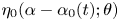 $\eta _0(\alpha -\alpha _0(t);\theta )$ and
 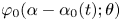 $\varphi _0(\alpha -\alpha _0(t);\theta )$ in the right-hand sides of (2.27) without changing
  $C_1$ would still lead to
  $\eta _t=0$,
  $\varphi _t=0$ and
  $\textrm{d}\kern0.7pt x_0/ \textrm {d} t=c$, and (2.25) would still give
  $\xi _t=c$. Including
  $-\alpha _0'(t)$ in
  $C_1$ leads instead to
 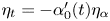 $\eta _t=-\alpha _0'(t)\eta _\alpha$ and
  $\varphi _t=-\alpha _0'(t)\varphi _\alpha$ in (2.27) and
 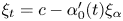 $\xi _t=c-\alpha _0'(t)\xi _\alpha$ in (2.25), which are satisfied by (A7). It also leads to
  $\textrm{d}\kern0.7pt x_0/ \textrm {d} t=[c-\alpha _0'(t)]$ in (2.26), which keeps the reconstruction of
  $\xi$ from
  $\eta$ via (2.13a,b) consistent with the evolution equation for
  $\xi _t$.
The functions in (A7) and (A8) are related by
 \begin{equation} \zeta(\alpha,t;\theta)=\alpha+\tilde\zeta(\alpha,\theta+k\alpha,t), \quad \varphi(\alpha,t;\theta)= \tilde\varphi(\alpha,\theta+k\alpha,t). \end{equation}
Applying the one-dimensional version of (2.27) to (A9) is equivalent to applying the torus version of (2.27) to (A8) and evaluating at  $(\alpha ,\theta +k\alpha ,t)$. Since (A7) satisfies the one-dimensional version of (2.27) and every point
  $(\alpha _1,\alpha _2)\in \mathbb{T}^2$ can be written as
  $(\alpha ,\theta +k\alpha )$ for some
  $\alpha$ and
  $\theta$, (A8) satisfies the torus version of (2.27).
Corollary A.5 Suppose  $\tilde \zeta _0(\alpha _1,\alpha _2)$,
  $\tilde \varphi _0(\alpha _1,\alpha _2)$,
  $\zeta _0(\alpha;\theta )$ and
  $\varphi _0(\alpha;\theta )$ satisfy the hypotheses of Theorem A.3 and
  $\xi _{0,\alpha }(\alpha;\theta )>0$ for
  $\alpha \in [0,2{\rm \pi} )$ and
  $\theta \in [0,2{\rm \pi} )$. Then if
  $C_1$ is chosen as in (2.28) to maintain
  $\tilde \xi (0,0,t)=0$, the solution of the torus version of (2.27) with initial conditions
 \begin{equation} \tilde\zeta(\alpha_1,\alpha_2,0) = \tilde\zeta_0(\alpha_1,\alpha_2), \quad \tilde\varphi(\alpha_1,\alpha_2,0) = \tilde\varphi_0(\alpha_1,\alpha_2), \end{equation}
has the form (A8) with
 \begin{equation} \alpha_0(t)=ct-\mathcal{A}_0({-}ct,-kct), \end{equation}
where  $\mathcal{A}_0(x_1,x_2)$ is defined implicitly by
 \begin{equation} \mathcal{A}_0(x_1,x_2) + \tilde\xi_0(x_1+\mathcal{A}_0(x_1,x_2), x_2+k\mathcal{A}_0(x_1,x_2)) = 0, \quad (x_1,x_2)\in\mathbb{T}^2. \end{equation}
Proof. The assumption that  $\xi _{0,\alpha }(\alpha;\theta )>0$ ensures that all the waves in the family
  $\zeta _0(\alpha;\theta )$ are single valued and have no vertical tangent lines. Under these hypotheses, it is proved in Wilkening & Zhao (Reference Wilkening and Zhao2020) that there is a unique function
  $\mathcal{A}_0(x_1,x_2)$ satisfying (A12) and that it is real analytic and periodic. We seek a solution of the form (A8) satisfying
  $\tilde \xi (0,0,t)=0$,
 \begin{align} \tilde\xi(0,0,t) &= \tilde\xi_0(-\alpha_0(t),-k\alpha_0(t)) +ct - \alpha_0(t) \nonumber\\ & = [ct-\alpha_0(t)] + \tilde\xi_0({-}ct+[ct-\alpha_0(t)], -kct+k[ct-\alpha_0(t)]) = 0. \end{align}
Comparing with (A12), we find that  $[ct-\alpha _0(t)]=\mathcal{A}_0(-ct,-kct)$, which is (A11). Since
  $\tilde \eta _0(\alpha _1,\alpha _2)$ is even,
  $\tilde \xi _0=H[\tilde \eta _0]$ is odd and
  $\mathcal{A}_0(0,0)=0$. Thus,
  $\alpha _0(0)=0$ and the initial conditions (A10) are satisfied. Since
  $\xi (0,0,t)=0$,
  $C_1$ satisfies (2.28).


 Open access