





1 Introduction
Canonical wall-bounded flows (channel, pipe and turbulent boundary layer (TBL)) are widely seen in engineering applications and in nature (Smits & Marusic Reference Smits and Marusic2013). Turbulent channel and pipe are internal flows driven by a pressure gradient, which fully determines the mean velocity profile (MVP) and hence also the friction coefficient. In contrast, the TBL, driven by the freestream, develops a profile dependent on both $x$
(streamwise) and
$x$
(streamwise) and $y$
(wall-normal) coordinates. These flows are of great theoretical and practical interest and have been studied for more than a century (Pope Reference Pope2000; Wilcox Reference Wilcox2006).
$y$
(wall-normal) coordinates. These flows are of great theoretical and practical interest and have been studied for more than a century (Pope Reference Pope2000; Wilcox Reference Wilcox2006).
A central issue in the study of these flows is to develop viable mathematical models, in particular, to predict the mean flow properties such as the MVP, mean kinetic-energy profile (MKP), mean temperature profile (MTP), etc. Despite intensive efforts, predictions have remained essentially empirical, with the exception of the log law for MVP in the so-called overlap region. In recent decades, large volumes of empirical data have been obtained from experimental and numerical studies, but they have not led to any deep understanding of the principles governing mean flow properties. Such principles, once discovered, should help to guide the statistical analysis of detailed data, offered particularly by direct numerical simulations (DNS). The present work develops new theoretical concepts aiming to discover physical principles, via an innovative symmetry approach.
The study of turbulence in canonical wall-bounded flows begins by a scaling analysis focusing on a one-dimensional variation with respect to distance from the wall (Pope Reference Pope2000). The analysis identifies friction velocity $u_{\unicode[STIX]{x1D70F}}$
, wall viscous length unit
$u_{\unicode[STIX]{x1D70F}}$
, wall viscous length unit $\unicode[STIX]{x1D6FF}_{\unicode[STIX]{x1D708}}\equiv \unicode[STIX]{x1D708}/u_{\unicode[STIX]{x1D70F}}$
and friction Reynolds number (Re)
$\unicode[STIX]{x1D6FF}_{\unicode[STIX]{x1D708}}\equiv \unicode[STIX]{x1D708}/u_{\unicode[STIX]{x1D70F}}$
and friction Reynolds number (Re) $Re_{\unicode[STIX]{x1D70F}}\equiv u_{\unicode[STIX]{x1D70F}}\unicode[STIX]{x1D6FF}/\unicode[STIX]{x1D708}$
as three fundamental physical parameters, where
$Re_{\unicode[STIX]{x1D70F}}\equiv u_{\unicode[STIX]{x1D70F}}\unicode[STIX]{x1D6FF}/\unicode[STIX]{x1D708}$
as three fundamental physical parameters, where $\unicode[STIX]{x1D6FF}$
is wall flow thickness (e.g. half-width of the channel or radius of the pipe, or thickness of the boundary layer) and
$\unicode[STIX]{x1D6FF}$
is wall flow thickness (e.g. half-width of the channel or radius of the pipe, or thickness of the boundary layer) and $\unicode[STIX]{x1D708}$
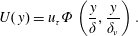
is kinematic viscosity. Scaling (dimensional) analysis yields an expression for the mean velocity as
$\unicode[STIX]{x1D708}$
is kinematic viscosity. Scaling (dimensional) analysis yields an expression for the mean velocity as
 $$\begin{eqnarray}U(\,y)=u_{\unicode[STIX]{x1D70F}}\unicode[STIX]{x1D6F7}\left(\frac{y}{\unicode[STIX]{x1D6FF}},\frac{y}{\unicode[STIX]{x1D6FF}_{\unicode[STIX]{x1D708}}}\right).\end{eqnarray}$$
In the limit $y/\unicode[STIX]{x1D6FF}\rightarrow 0$
(very close to the wall),
$y/\unicode[STIX]{x1D6FF}\rightarrow 0$
(very close to the wall), $\unicode[STIX]{x1D6F7}(y/\unicode[STIX]{x1D6FF},y/\unicode[STIX]{x1D6FF}_{\unicode[STIX]{x1D708}})\rightarrow \unicode[STIX]{x1D6F7}_{1}(0,y/\unicode[STIX]{x1D6FF}_{\unicode[STIX]{x1D708}})=f_{w}(y^{+})$
, which is called wall function, first used by Prandtl (Reference Prandtl1925), and
$\unicode[STIX]{x1D6F7}(y/\unicode[STIX]{x1D6FF},y/\unicode[STIX]{x1D6FF}_{\unicode[STIX]{x1D708}})\rightarrow \unicode[STIX]{x1D6F7}_{1}(0,y/\unicode[STIX]{x1D6FF}_{\unicode[STIX]{x1D708}})=f_{w}(y^{+})$
, which is called wall function, first used by Prandtl (Reference Prandtl1925), and $y^{+}=y/\unicode[STIX]{x1D6FF}_{\unicode[STIX]{x1D708}}$
, is the distance in wall units. In the other limit
$y^{+}=y/\unicode[STIX]{x1D6FF}_{\unicode[STIX]{x1D708}}$
, is the distance in wall units. In the other limit $y/\unicode[STIX]{x1D6FF}_{\unicode[STIX]{x1D708}}\gg 1$
(very far from the wall),
$y/\unicode[STIX]{x1D6FF}_{\unicode[STIX]{x1D708}}\gg 1$
(very far from the wall), $\unicode[STIX]{x1D6F7}(y/\unicode[STIX]{x1D6FF},y/\unicode[STIX]{x1D6FF}_{\unicode[STIX]{x1D708}})\rightarrow \unicode[STIX]{x1D6F7}_{1}(y/\unicode[STIX]{x1D6FF},\infty )=g(y^{\prime })$
with
$\unicode[STIX]{x1D6F7}(y/\unicode[STIX]{x1D6FF},y/\unicode[STIX]{x1D6FF}_{\unicode[STIX]{x1D708}})\rightarrow \unicode[STIX]{x1D6F7}_{1}(y/\unicode[STIX]{x1D6FF},\infty )=g(y^{\prime })$
with $y^{\prime }=y/\unicode[STIX]{x1D6FF}$
, which is commonly referred to as the outer function. Until now, the actual forms of
$y^{\prime }=y/\unicode[STIX]{x1D6FF}$
, which is commonly referred to as the outer function. Until now, the actual forms of $f_{w}(y^{+})$
and
$f_{w}(y^{+})$
and $g(y^{\prime })$
are based on empirical propositions. The most popular model for the wall function is given by Van Driest (Reference Driest1956), which is believed to be universal for incompressible canonical wall-bounded flows, whereas the form of the wake function is more varied, depending on the geometry and other physical conditions. Specifically, a velocity-defect law due to Von Karman (Reference Von Karman1930) reads
$g(y^{\prime })$
are based on empirical propositions. The most popular model for the wall function is given by Van Driest (Reference Driest1956), which is believed to be universal for incompressible canonical wall-bounded flows, whereas the form of the wake function is more varied, depending on the geometry and other physical conditions. Specifically, a velocity-defect law due to Von Karman (Reference Von Karman1930) reads
 $$\begin{eqnarray}U_{d}^{+}(\,y/\unicode[STIX]{x1D6FF})=U_{c}^{+}-U_{}^{+}(\,y/\unicode[STIX]{x1D6FF})=F_{D}(\,y/\unicode[STIX]{x1D6FF}),\end{eqnarray}$$
where $U_{d}^{+}$
is the mean velocity defect,
$U_{d}^{+}$
is the mean velocity defect, $U_{c}^{+}$
is the centreline velocity for channel and pipe flows, or velocity at the edge of the TBL (typically 99 % of the freestream velocity), while the outer function
$U_{c}^{+}$
is the centreline velocity for channel and pipe flows, or velocity at the edge of the TBL (typically 99 % of the freestream velocity), while the outer function $F_{D}$
is flow dependent (superscript
$F_{D}$
is flow dependent (superscript $+$
indicates normalization using
$+$
indicates normalization using $u_{\unicode[STIX]{x1D70F}}$
and
$u_{\unicode[STIX]{x1D70F}}$
and $\unicode[STIX]{x1D708}$
, i.e. in wall units).
$\unicode[STIX]{x1D708}$
, i.e. in wall units).
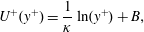
The above two-scale (inner and outer) description follows the essence of Prandtl’s boundary-layer concept and is commonly referred to as ‘classical’ scaling. The celebrated log law is obtained by matching (1.1) and (1.2), that is
 $$\begin{eqnarray}U^{+}(y^{+})=\frac{1}{\unicode[STIX]{x1D705}}\ln (y^{+})+B,\end{eqnarray}$$
where the Karman constant $\unicode[STIX]{x1D705}$
was believed to be universal (Pope Reference Pope2000; Wilcox Reference Wilcox2006), and the additive constant
$\unicode[STIX]{x1D705}$
was believed to be universal (Pope Reference Pope2000; Wilcox Reference Wilcox2006), and the additive constant $B$
is flow dependent (Marusic et al.
Reference Marusic, McKeon, Monkewitz, Nagib, Smits and Sreenivasan2010). The log law was later obtained by Millikan (Reference Millikan1938) by an argument that
$B$
is flow dependent (Marusic et al.
Reference Marusic, McKeon, Monkewitz, Nagib, Smits and Sreenivasan2010). The log law was later obtained by Millikan (Reference Millikan1938) by an argument that $y^{+}\unicode[STIX]{x2202}U^{+}/\unicode[STIX]{x2202}y^{+}$
must match using (1.1) and (1.2). However, other quantities can be invoked to define the matching condition. For instance, if one invokes
$y^{+}\unicode[STIX]{x2202}U^{+}/\unicode[STIX]{x2202}y^{+}$
must match using (1.1) and (1.2). However, other quantities can be invoked to define the matching condition. For instance, if one invokes $(\,y^{+}/U^{+})\unicode[STIX]{x2202}U^{+}/\unicode[STIX]{x2202}y^{+}$
as an invariant matching condition, the resulting functional form of the mean velocity is a power law. Thus, (1.3) is not the unique matching form and that is why the debate between the log law and the power law has been strong over the decades (Barenblatt Reference Barenblatt1993; Cipra Reference Cipra1996; Barenblatt & Chorin Reference Barenblatt and Chorin2004; George Reference George2005).
$(\,y^{+}/U^{+})\unicode[STIX]{x2202}U^{+}/\unicode[STIX]{x2202}y^{+}$
as an invariant matching condition, the resulting functional form of the mean velocity is a power law. Thus, (1.3) is not the unique matching form and that is why the debate between the log law and the power law has been strong over the decades (Barenblatt Reference Barenblatt1993; Cipra Reference Cipra1996; Barenblatt & Chorin Reference Barenblatt and Chorin2004; George Reference George2005).
In turbulent-pipe studies, the log law contradicts the boundary conditions at wall and centreline, and Prandtl was dissatisfied with this (Davidson et al.
Reference Davidson, Kaneda, Moffatt and Sreenivasan2011). In 1925, Prandtl suggested representing effects of turbulent fluctuation, i.e. Reynolds stress $W=-\langle u^{\prime }v^{\prime }\rangle$
(which is non-negative in turbulent shear flows except in the case of negative production due to alignment of successive coherent structure orientations at a physical location (Hussain & Zaman Reference Hussain and Zaman1985), which is not a subject of concern here), in terms of an eddy viscosity
$W=-\langle u^{\prime }v^{\prime }\rangle$
(which is non-negative in turbulent shear flows except in the case of negative production due to alignment of successive coherent structure orientations at a physical location (Hussain & Zaman Reference Hussain and Zaman1985), which is not a subject of concern here), in terms of an eddy viscosity $\unicode[STIX]{x1D708}_{T}$
and a velocity gradient, that is
$\unicode[STIX]{x1D708}_{T}$
and a velocity gradient, that is
 $$\begin{eqnarray}-\langle u^{\prime }v^{\prime }\rangle =\unicode[STIX]{x1D708}_{T}S=\ell _{uv}^{2}S^{2}.\end{eqnarray}$$
Here, $S=\unicode[STIX]{x2202}U/\unicode[STIX]{x2202}y$
is the mean shear and
$S=\unicode[STIX]{x2202}U/\unicode[STIX]{x2202}y$
is the mean shear and
 $$\begin{eqnarray}\ell _{uv}=\sqrt{W}/S\end{eqnarray}$$
is called the stress length function, which is the same as the mixing length $\ell _{M}$
introduced by Prandtl (Reference Prandtl1925), but now interpreted as indicating an eddy whose size does not need to be proportional to
$\ell _{M}$
introduced by Prandtl (Reference Prandtl1925), but now interpreted as indicating an eddy whose size does not need to be proportional to $y$
(the basis of the classical mixing length hypothesis). Note that (1.4) is a mere definition, which requires
$y$
(the basis of the classical mixing length hypothesis). Note that (1.4) is a mere definition, which requires $\ell _{uv}$
to be modelled. As summarized in White (Reference White2006), both Prandtl (Reference Prandtl1925) and Von Karman (Reference Von Karman1930) took turns to make estimates of
$\ell _{uv}$
to be modelled. As summarized in White (Reference White2006), both Prandtl (Reference Prandtl1925) and Von Karman (Reference Von Karman1930) took turns to make estimates of $\ell _{uv}$
and arrived at the following proposals:
$\ell _{uv}$
and arrived at the following proposals:
 $$\begin{eqnarray}\displaystyle & \text{overlap region}\quad \ell _{uv}\approx \unicode[STIX]{x1D705}y & \displaystyle\end{eqnarray}$$
 $$\begin{eqnarray}\displaystyle & \text{sublayer}\quad \ell _{uv}\approx y^{2} & \displaystyle\end{eqnarray}$$
 $$\begin{eqnarray}\displaystyle & \text{outer layer}\quad \ell _{uv}\approx \text{const.} & \displaystyle\end{eqnarray}$$
The linear assumption (1.6) leads to the log law, while (1.7) is proposed to satisfy the wall condition, i.e. $\ell _{uv}\rightarrow 0$
as
$\ell _{uv}\rightarrow 0$
as $y\rightarrow 0$
(because of the vanishing Reynolds stress
$y\rightarrow 0$
(because of the vanishing Reynolds stress $W=0$
and the non-zero mean shear
$W=0$
and the non-zero mean shear $S=u_{\unicode[STIX]{x1D70F}}^{2}/\unicode[STIX]{x1D708}$
at the wall Pope Reference Pope2000). Various combinations of (1.6)–(1.8) yield formulas for wall function and wake function. For example, by assuming both (1.6) and (1.7), van Driest (Reference Driest1956) proposed an exponential damping function
$S=u_{\unicode[STIX]{x1D70F}}^{2}/\unicode[STIX]{x1D708}$
at the wall Pope Reference Pope2000). Various combinations of (1.6)–(1.8) yield formulas for wall function and wake function. For example, by assuming both (1.6) and (1.7), van Driest (Reference Driest1956) proposed an exponential damping function
 $$\begin{eqnarray}\ell _{uv}\approx \unicode[STIX]{x1D705}y[1-\exp (-y^{+}/A)],\end{eqnarray}$$
where $A\approx 26$
is determined for a flat-plate TBL. One may also merge (1.9) with (1.8) to produce a piecewise functional form covering both inner and outer flows, widely used in Reynolds-averaged Navier–Stokes (RANS) models (Pope Reference Pope2000; Wilcox Reference Wilcox2006). Another well-known model was suggested by Coles (Reference Coles1956) going from the overlap region (the log law) to the outer region, by taking into account both (1.2) and (1.3), namely
$A\approx 26$
is determined for a flat-plate TBL. One may also merge (1.9) with (1.8) to produce a piecewise functional form covering both inner and outer flows, widely used in Reynolds-averaged Navier–Stokes (RANS) models (Pope Reference Pope2000; Wilcox Reference Wilcox2006). Another well-known model was suggested by Coles (Reference Coles1956) going from the overlap region (the log law) to the outer region, by taking into account both (1.2) and (1.3), namely
 $$\begin{eqnarray}U^{+}(y^{+})=\frac{1}{\unicode[STIX]{x1D705}}\ln (y^{+})+B+\frac{2\unicode[STIX]{x1D6F1}_{c}}{\unicode[STIX]{x1D705}}W_{f}\left(\frac{y}{\unicode[STIX]{x1D6FF}}\right),\end{eqnarray}$$
with the Coles wake parameter $\unicode[STIX]{x1D6F1}_{c}$
and the wake function
$\unicode[STIX]{x1D6F1}_{c}$
and the wake function $W_{f}(x)$
. A widely used empirical model for pipe or channel or TBL is
$W_{f}(x)$
. A widely used empirical model for pipe or channel or TBL is $W_{f}(x)=\sin ^{2}(\unicode[STIX]{x03C0}x/2)$
.
$W_{f}(x)=\sin ^{2}(\unicode[STIX]{x03C0}x/2)$
.
As we show below, the correct scaling in the viscous sublayer is $\ell _{uv}\propto y^{3/2}$
and (1.7) describes the scaling in the buffer layer. The latter, placed just above the viscous sublayer, is populated with numerous near-wall vortex structures and where turbulent production is the strongest. These two features distinguish them from the sublayer. Note that although eddy viscosity/mixing length approaches have made some modest successes, these cannot be taken literally as they are not supposed to be. For example, equation (1.6) cannot be valid very far from the wall. In order to describe the MVP for the entire flow region and to accurately measure flow constants (such as
$\ell _{uv}\propto y^{3/2}$
and (1.7) describes the scaling in the buffer layer. The latter, placed just above the viscous sublayer, is populated with numerous near-wall vortex structures and where turbulent production is the strongest. These two features distinguish them from the sublayer. Note that although eddy viscosity/mixing length approaches have made some modest successes, these cannot be taken literally as they are not supposed to be. For example, equation (1.6) cannot be valid very far from the wall. In order to describe the MVP for the entire flow region and to accurately measure flow constants (such as $\unicode[STIX]{x1D705}$
), we need to theoretically determine the stress length function for the entire flow. We also need theoretical arguments to extend/modify the function to include other boundary conditions (such as pressure gradient, roughness, heating, etc.).
$\unicode[STIX]{x1D705}$
), we need to theoretically determine the stress length function for the entire flow. We also need theoretical arguments to extend/modify the function to include other boundary conditions (such as pressure gradient, roughness, heating, etc.).
Two important issues are worth mentioning: how exact is the log law and how universal is the Karman constant $\unicode[STIX]{x1D705}$
? The log law has been challenged by Barenblatt (Reference Barenblatt1993), Barenblatt & Chorin (Reference Barenblatt and Chorin2004) and George (Reference George2005). They argue that the power law is more natural and fits the MVP data in a wider domain. In addition,
$\unicode[STIX]{x1D705}$
? The log law has been challenged by Barenblatt (Reference Barenblatt1993), Barenblatt & Chorin (Reference Barenblatt and Chorin2004) and George (Reference George2005). They argue that the power law is more natural and fits the MVP data in a wider domain. In addition, $\unicode[STIX]{x1D705}$
has been assumed to be a universal constant for a long time (Pope Reference Pope2000; Wilcox Reference Wilcox2006), equaling 0.40–0.41. However, as more data accumulate,
$\unicode[STIX]{x1D705}$
has been assumed to be a universal constant for a long time (Pope Reference Pope2000; Wilcox Reference Wilcox2006), equaling 0.40–0.41. However, as more data accumulate, $\unicode[STIX]{x1D705}$
measured using the classical definition of the log law (1.3) shows a 20 % variation, from 0.37 to 0.45 (Nagib & Chauhan Reference Nagib and Chauhan2008; Marusic et al.
Reference Marusic, McKeon, Monkewitz, Nagib, Smits and Sreenivasan2010; Segalini, Orlu & Alfredsson Reference Segalini, Orlu and Alfredsson2013; Wu et al.
Reference Wu, Chen, She and Hussain2013). To resolve these controversies, Smits, McKeon & Marusic (Reference Smits, McKeon and Marusic2011) suggest developing new facilities with an improved measurement accuracy; also, a valuable move would be to develop a composite description of MVP, such as the models by Monkewitz, Chauhan & Nagib (Reference Monkewitz, Chauhan and Nagib2007) (hereafter cited as MCN) and Nagib & Chauhan (Reference Nagib and Chauhan2008). Further improved models should involve more relevant physical content and more rigorous theoretical underpinning.
$\unicode[STIX]{x1D705}$
measured using the classical definition of the log law (1.3) shows a 20 % variation, from 0.37 to 0.45 (Nagib & Chauhan Reference Nagib and Chauhan2008; Marusic et al.
Reference Marusic, McKeon, Monkewitz, Nagib, Smits and Sreenivasan2010; Segalini, Orlu & Alfredsson Reference Segalini, Orlu and Alfredsson2013; Wu et al.
Reference Wu, Chen, She and Hussain2013). To resolve these controversies, Smits, McKeon & Marusic (Reference Smits, McKeon and Marusic2011) suggest developing new facilities with an improved measurement accuracy; also, a valuable move would be to develop a composite description of MVP, such as the models by Monkewitz, Chauhan & Nagib (Reference Monkewitz, Chauhan and Nagib2007) (hereafter cited as MCN) and Nagib & Chauhan (Reference Nagib and Chauhan2008). Further improved models should involve more relevant physical content and more rigorous theoretical underpinning.
Here we pursue this line of thought by developing a composite formula connecting the inner and outer (and hence the overlap) flow region descriptions guided by a dilatation-invariance principle. Specifically, we determine the forms of $f_{w}(\,y^{+})$
and
$f_{w}(\,y^{+})$
and $g(\,y^{\prime })$
(
$g(\,y^{\prime })$
( $\unicode[STIX]{x1D705}$
is measured based on
$\unicode[STIX]{x1D705}$
is measured based on $g$
), and then the entire function
$g$
), and then the entire function $\unicode[STIX]{x1D6F7}(\,y^{\prime },y^{+})$
. This is accomplished by introducing a set of new quantities, called order functions, which is an extension of the concept of order parameter in Landau’s mean-field theory to reveal the macroscopic symmetry emerged from microscopic fluctuations. Here, the order function is different from the order parameter in its spatial variation in the wall normal direction, which reflects the changing of symmetry due to varying turbulent fluctuations. Briefly, our derivation of the MVP involves three steps. First, the stress length function is identified as the order function (other choices such as the mean velocity or the eddy viscosity function are inappropriate as discussed below), which characterizes the length scale of eddies responsible for the momentum transport normal to the wall. Second, a dilatation-group analysis is applied to the mean-momentum equation, focusing on the dilatation invariants of the stress length function and its derivative as (new) similarity variables (note that the group invariants include dimensionless quantities as a special set), which further leads to building local invariant solutions for the unclosed balance equations. Third, a multi-layer formula for the stress length function over the entire flow domain is developed employing the multiplicative rule; and the balance mechanisms between different terms in the turbulent kinetic-energy equation are interpreted as the origin of the multi-layer structure. That is, the transition from one layer to another is assumed to satisfy a generalized Lie-group invariance ansatz so that the matching technique yields a complete analytical formula. Hence it yields the MVP for the entire flow, where
$\unicode[STIX]{x1D6F7}(\,y^{\prime },y^{+})$
. This is accomplished by introducing a set of new quantities, called order functions, which is an extension of the concept of order parameter in Landau’s mean-field theory to reveal the macroscopic symmetry emerged from microscopic fluctuations. Here, the order function is different from the order parameter in its spatial variation in the wall normal direction, which reflects the changing of symmetry due to varying turbulent fluctuations. Briefly, our derivation of the MVP involves three steps. First, the stress length function is identified as the order function (other choices such as the mean velocity or the eddy viscosity function are inappropriate as discussed below), which characterizes the length scale of eddies responsible for the momentum transport normal to the wall. Second, a dilatation-group analysis is applied to the mean-momentum equation, focusing on the dilatation invariants of the stress length function and its derivative as (new) similarity variables (note that the group invariants include dimensionless quantities as a special set), which further leads to building local invariant solutions for the unclosed balance equations. Third, a multi-layer formula for the stress length function over the entire flow domain is developed employing the multiplicative rule; and the balance mechanisms between different terms in the turbulent kinetic-energy equation are interpreted as the origin of the multi-layer structure. That is, the transition from one layer to another is assumed to satisfy a generalized Lie-group invariance ansatz so that the matching technique yields a complete analytical formula. Hence it yields the MVP for the entire flow, where $f_{w}(\,y^{+})$
and
$f_{w}(\,y^{+})$
and $g(\,y^{\prime })$
are also derived in good agreement with the data.
$g(\,y^{\prime })$
are also derived in good agreement with the data.
Note that the current analysis focuses on the group invariants of the stress length function instead of the mean velocity in earlier works by Oberlack (Reference Oberlack2001), Lindgren, Osterlund & Johansson (Reference Lindgren, Osterlund and Johansson2004) and Marati et al. (Reference Marati, Davoudi, Casciola and Eckhardt2006), explained as follows. In our view, it is very important to choose the right group invariant when its constancy is used to construct the invariant solution. The constant dilatation invariant for the mean velocity, as assumed in previous works, is only valid in part of the viscous sublayer very close to the wall where $U^{+}\approx y^{+}$
; and this constancy is lost except in a restricted region beyond the log layer where Barenblatt argued it is the power law (Barenblatt Reference Barenblatt1993). However, Barenblatt’s proposal has two difficulties: on one hand, there exists no simple pattern for the variation of the dilatation invariant of the mean velocity from one layer to another (so as to define a multi-layer); on the other hand, the invariant (e.g. scaling exponent) is
$U^{+}\approx y^{+}$
; and this constancy is lost except in a restricted region beyond the log layer where Barenblatt argued it is the power law (Barenblatt Reference Barenblatt1993). However, Barenblatt’s proposal has two difficulties: on one hand, there exists no simple pattern for the variation of the dilatation invariant of the mean velocity from one layer to another (so as to define a multi-layer); on the other hand, the invariant (e.g. scaling exponent) is $Re$
-dependent, making this proposal less sound. As we show below, both difficulties can be resolved when one chooses the dilatation invariants of the stress length (order) function and its derivative: a clear and universal multi-layer structure appears with
$Re$
-dependent, making this proposal less sound. As we show below, both difficulties can be resolved when one chooses the dilatation invariants of the stress length (order) function and its derivative: a clear and universal multi-layer structure appears with $Re$
-independent scaling. It turns out that the correct choice of dilatation invariants is key to constructing the composite solution matching two local invariant solutions of adjacent layers together, a previously unresolved issue (Oberlack & Rosteck Reference Oberlack and Rosteck2010).
$Re$
-independent scaling. It turns out that the correct choice of dilatation invariants is key to constructing the composite solution matching two local invariant solutions of adjacent layers together, a previously unresolved issue (Oberlack & Rosteck Reference Oberlack and Rosteck2010).
The present analysis can be considered as a generalization of the intermediate asymptotic approach by Barenblatt (Reference Barenblatt1996), who proposes the existence of local power law in a restricted domain. Presently, the sublayer and buffer layer are restricted, respectively, to the domains of $y^{+}\lesssim 10$
and
$y^{+}\lesssim 10$
and $10\lesssim y^{+}\lesssim 40$
. The novelty here is to motivate three concrete analytical forms of Lie-group invariance ansatz (see (2.21), (2.24) and (2.26)). In particular, neither the defect-power law (2.24) nor the transition from one scaling to another (2.26) has been obtained before; these yield the analytical function for the stress length valid throughout the entire flow region. In other words, the present formalism gives the inner wall function and outer wake function in the classical boundary layer asymptotic sense (as
$10\lesssim y^{+}\lesssim 40$
. The novelty here is to motivate three concrete analytical forms of Lie-group invariance ansatz (see (2.21), (2.24) and (2.26)). In particular, neither the defect-power law (2.24) nor the transition from one scaling to another (2.26) has been obtained before; these yield the analytical function for the stress length valid throughout the entire flow region. In other words, the present formalism gives the inner wall function and outer wake function in the classical boundary layer asymptotic sense (as $Re_{\unicode[STIX]{x1D70F}}\rightarrow \infty$
), without adopting the restrictive Baranblatt’s intermediate asymptotic argument. Also note that the current symmetry analysis is significantly different from previous works modelling the mean velocity (Nickels Reference Nickels2004; Del Alamo & Jimenez Reference Del Alamo and Jimenez2006; Monkewitz et al.
Reference Monkewitz, Chauhan and Nagib2007; Panton Reference Panton2007; L’vov, Procaccia & Rudenko Reference L’vov, Procaccia and Rudenko2008) by two features: a unified description of the mean velocities of all three canonical flows (channel, pipe and TBL) is obtained for the first time and the current parameters adequately characterize the physical multi-layer structure in the flow. This symmetry may be a physical principle applicable to a variety of wall-bounded flows, for which no-slip wall is a common presence and the multi-layer structure is a universal characteristic. Several other examples, such as rough pipe (She et al.
Reference She, Wu, Chen and Hussain2012), compressible TBL (Wu et al.
Reference Wu, Bi, Hussain and She2017), etc., show convincing evidence of the multi-layer structure. In summary, we have achieved a fairly accurate description, beyond the log law and power law, of the entire mean profiles of wall turbulent flow.
$Re_{\unicode[STIX]{x1D70F}}\rightarrow \infty$
), without adopting the restrictive Baranblatt’s intermediate asymptotic argument. Also note that the current symmetry analysis is significantly different from previous works modelling the mean velocity (Nickels Reference Nickels2004; Del Alamo & Jimenez Reference Del Alamo and Jimenez2006; Monkewitz et al.
Reference Monkewitz, Chauhan and Nagib2007; Panton Reference Panton2007; L’vov, Procaccia & Rudenko Reference L’vov, Procaccia and Rudenko2008) by two features: a unified description of the mean velocities of all three canonical flows (channel, pipe and TBL) is obtained for the first time and the current parameters adequately characterize the physical multi-layer structure in the flow. This symmetry may be a physical principle applicable to a variety of wall-bounded flows, for which no-slip wall is a common presence and the multi-layer structure is a universal characteristic. Several other examples, such as rough pipe (She et al.
Reference She, Wu, Chen and Hussain2012), compressible TBL (Wu et al.
Reference Wu, Bi, Hussain and She2017), etc., show convincing evidence of the multi-layer structure. In summary, we have achieved a fairly accurate description, beyond the log law and power law, of the entire mean profiles of wall turbulent flow.
This paper is organized as follows. In § 2, we summarize previous studies using Lie group symmetry analysis and introduce our study of invariant solutions of stress length function with three ansatz. In § 3, we apply the analysis to form a concise description of the wall function with viscous sublayer, buffer layer, log layer and the wake function consisting of a bulk layer; for turbulent pipes and channels the wake also consists of a core layer. Section 4 is devoted to comparing the theoretical results and the empirical data. Section 5 summarizes and further discusses the results. In appendix A, we present a standard three-step Lie-group-symmetry analysis, so that no previous knowledge of Lie group is assumed. For more exhaustive discussions, see Bluman & Kumei (1989) and Cantwell (Reference Cantwell2002). In appendix B, we discuss the main features of a current symmetry-based approach and its generality to other wall flows.
2 Symmetry approach to the study of wall flows
Symmetry is an important concept in physics (Falkovich Reference Falkovich2009; Gibson, Halcrow & Cvitanovic Reference Gibson, Halcrow and Cvitanovic2009; Kadanoff Reference Kadanoff2009) as it indicates invariants in the system. It is associated with a pattern which satisfies invariant properties under a certain rule of transformation. Generally speaking, if there is an invariant quantity, i.e. remaining unchanged under transformation, then there exists a symmetry. Lie groups are basic tools to characterize continuous symmetry in mathematical structures such as differential equations. It was originally developed by Sophus Lie in the 1890s (Bluman & Kumei 1989; Cantwell Reference Cantwell2002), laying the foundations for the theory of continuous transformation groups and now provides a systematic tool to reduce the differential order or the number of independent variables, when studying ordinary or partial differential equations.
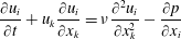
Early studies devoted to Lie-group symmetry analysis for the Navier–Stokes (NS) equations, i.e.
 $$\begin{eqnarray}\displaystyle & \displaystyle \frac{\unicode[STIX]{x2202}u_{k}}{\unicode[STIX]{x2202}x_{k}}=0 & \displaystyle\end{eqnarray}$$
 $$\begin{eqnarray}\displaystyle & \displaystyle \frac{\unicode[STIX]{x2202}u_{i}}{\unicode[STIX]{x2202}t}+u_{k}\frac{\unicode[STIX]{x2202}u_{i}}{\unicode[STIX]{x2202}x_{k}}=\unicode[STIX]{x1D708}\frac{\unicode[STIX]{x2202}^{2}u_{i}}{\unicode[STIX]{x2202}x_{k}^{2}}-\frac{\unicode[STIX]{x2202}p}{\unicode[STIX]{x2202}x_{i}} & \displaystyle\end{eqnarray}$$
(note that the density is absorbed in $p$
) and the relevant symmetry transformations can be found in textbooks, for example, Frisch (Reference Frisch1995) and Cantwell (Reference Cantwell2002), which are briefly summarized below:
$p$
) and the relevant symmetry transformations can be found in textbooks, for example, Frisch (Reference Frisch1995) and Cantwell (Reference Cantwell2002), which are briefly summarized below:
 $$\begin{eqnarray}\left.\begin{array}{@{}l@{}}\!(\text{i})\;\text{space translations:}\;t^{\ast }=t,\quad x_{i}^{\ast }=x_{i}+\unicode[STIX]{x1D716}_{i},\quad u_{i}^{\ast }=u_{i},\quad p^{\ast }=p\!\\ \!(\text{ii})\;\text{time translations:}\;t^{\ast }=t+\unicode[STIX]{x1D716},\quad x_{i}^{\ast }=x_{i},\quad u_{i}^{\ast }=u_{i},\quad p^{\ast }=p\!\\ \!(\text{iii})\;\text{Galilean transformations:}\;t^{\ast }=t,\quad x_{i}^{\ast }=x_{i}+\unicode[STIX]{x1D716}_{i}t,\quad u_{i}^{\ast }=u_{i}+\unicode[STIX]{x1D716}_{i},\quad p^{\ast }=p\!\\ \!(\text{iv})\;\text{rotations:}\;t^{\ast }=t,\quad x_{i}^{\ast }=a_{ij}x_{j},\quad u_{i}^{\ast }=a_{ij}u_{j},\quad p^{\ast }=p\!\\ \!(\text{v})\;\text{dilatations:}\;t^{\ast }=\text{e}^{\unicode[STIX]{x1D716}}t,\quad x_{i}^{\ast }=\text{e}^{\unicode[STIX]{x1D706}\unicode[STIX]{x1D716}}x_{i},\quad u_{i}^{\ast }=\text{e}^{(\unicode[STIX]{x1D706}-1)\unicode[STIX]{x1D716}}u_{i},\quad \unicode[STIX]{x1D708}^{\ast }=\text{e}^{(2\unicode[STIX]{x1D706}-1)\unicode[STIX]{x1D716}}\unicode[STIX]{x1D708},\quad p^{\ast }=\text{e}^{(2\unicode[STIX]{x1D706}-1)\unicode[STIX]{x1D716}}p.\!\end{array}\right\}\end{eqnarray}$$
Here $\unicode[STIX]{x1D716}\in R$
(and
$\unicode[STIX]{x1D716}\in R$
(and $\unicode[STIX]{x1D716}_{i}\in R^{3}$
) denotes the Lie-group parameter;
$\unicode[STIX]{x1D716}_{i}\in R^{3}$
) denotes the Lie-group parameter; $a_{ij}$
is the element of an orthonormal matrix (the reflection symmetry is also included);
$a_{ij}$
is the element of an orthonormal matrix (the reflection symmetry is also included); $\unicode[STIX]{x1D706}\in R$
is a free parameter for dilatations (dilatation on viscosity also;
$\unicode[STIX]{x1D706}\in R$
is a free parameter for dilatations (dilatation on viscosity also; $\unicode[STIX]{x1D706}=1/2$
if no dilatation of viscosity). Note that the boundary condition is crucial for the application of symmetry transformations, because it may break the aforementioned symmetries in (2.3) or introduce new symmetries (Bluman & Kumei 1989; Kelbin, Cheviakov & Oberlack Reference Kelbin, Cheviakov and Oberlack2013; Avsarkisov, Oberlack & Hoyas Reference Avsarkisov, Oberlack and Hoyas2014; Chen & Hussain Reference Chen and Hussain2017).
$\unicode[STIX]{x1D706}=1/2$
if no dilatation of viscosity). Note that the boundary condition is crucial for the application of symmetry transformations, because it may break the aforementioned symmetries in (2.3) or introduce new symmetries (Bluman & Kumei 1989; Kelbin, Cheviakov & Oberlack Reference Kelbin, Cheviakov and Oberlack2013; Avsarkisov, Oberlack & Hoyas Reference Avsarkisov, Oberlack and Hoyas2014; Chen & Hussain Reference Chen and Hussain2017).
Symmetry analysis is a particularly useful tool in the study of turbulence. For example, the Kolmogorov 1941 theory (Kolmogorov Reference Kolmogorov1941), the Frisch–Parisi multi-fractal model (Frisch & Parisi Reference Frisch, Parisi, Ghil, Benzi and Parisi1985), as well as the She–Leveque model of intermittency (She & Leveque Reference She and Leveque1994; She & Zhang Reference She and Zhang2009) are all based on symmetry considerations. The symmetry can be formally defined: if $\boldsymbol{u}(t,\boldsymbol{x})$
is a solution for a velocity field, then the transformed
$\boldsymbol{u}(t,\boldsymbol{x})$
is a solution for a velocity field, then the transformed $\boldsymbol{u}^{\ast }(t^{\ast },\boldsymbol{x}^{\ast })$
is also a solution (
$\boldsymbol{u}^{\ast }(t^{\ast },\boldsymbol{x}^{\ast })$
is also a solution ( $\ast$
denotes transformed variables). In general, the velocity field
$\ast$
denotes transformed variables). In general, the velocity field $\boldsymbol{u}(t,\boldsymbol{x})$
could have the following symmetries for each of the above items in (2.3): (i–ii) homogeneity in space and time; (iii) independent of reference frame (note, however, that acceleration is permitted); (iv) isotropy: isotropic turbulence with zero mean velocity; and (v) Re similarity for
$\boldsymbol{u}(t,\boldsymbol{x})$
could have the following symmetries for each of the above items in (2.3): (i–ii) homogeneity in space and time; (iii) independent of reference frame (note, however, that acceleration is permitted); (iv) isotropy: isotropic turbulence with zero mean velocity; and (v) Re similarity for $\unicode[STIX]{x1D706}=1/2$
(constant viscosity). The three scaling models mentioned above (Kolmogorov Reference Kolmogorov1941; Frisch & Parisi Reference Frisch, Parisi, Ghil, Benzi and Parisi1985; She & Leveque Reference She and Leveque1994) impose appropriate symmetry constraints on turbulent fluctuating velocities in the scale space to predict the scaling of a two-point velocity structure function. This work is a continuing effort in the same direction, but directs the subject from homogeneous isotropic turbulence to wall flows as well as from scale space to physical space, as described below.
$\unicode[STIX]{x1D706}=1/2$
(constant viscosity). The three scaling models mentioned above (Kolmogorov Reference Kolmogorov1941; Frisch & Parisi Reference Frisch, Parisi, Ghil, Benzi and Parisi1985; She & Leveque Reference She and Leveque1994) impose appropriate symmetry constraints on turbulent fluctuating velocities in the scale space to predict the scaling of a two-point velocity structure function. This work is a continuing effort in the same direction, but directs the subject from homogeneous isotropic turbulence to wall flows as well as from scale space to physical space, as described below.
2.1 Symmetry analysis with length (order) functions
Let us take a canonical turbulent channel flow in the $x$
direction, for example. The mean-momentum equation has the following form, steady in time,
$x$
direction, for example. The mean-momentum equation has the following form, steady in time,
 $$\begin{eqnarray}\frac{\unicode[STIX]{x2202}}{\unicode[STIX]{x2202}y}\left(\ell _{uv}\frac{\unicode[STIX]{x2202}U}{\unicode[STIX]{x2202}y}\right)^{2}+\unicode[STIX]{x1D708}\frac{\unicode[STIX]{x2202}^{2}U}{\unicode[STIX]{x2202}y^{2}}+\bar{P}_{x}=0,\end{eqnarray}$$
where $\bar{P}_{x}$
is the constant pressure gradient driving the channel flow; the nonlinear mean convection term and the diffusion terms in
$\bar{P}_{x}$
is the constant pressure gradient driving the channel flow; the nonlinear mean convection term and the diffusion terms in $x$
and
$x$
and $z$
directions are all zeros. In (2.4), the Reynolds stress is replaced by the stress length function, e.g. (1.5). In the following, we treat (2.4) for inner and outer flows separately (as in a standard singular perturbation framework). For the inner flow, using viscous (wall) units, i.e.
$z$
directions are all zeros. In (2.4), the Reynolds stress is replaced by the stress length function, e.g. (1.5). In the following, we treat (2.4) for inner and outer flows separately (as in a standard singular perturbation framework). For the inner flow, using viscous (wall) units, i.e.
 $$\begin{eqnarray}y^{+}=yu_{\unicode[STIX]{x1D70F}}/\unicode[STIX]{x1D708},\quad U^{+}=U/u_{\unicode[STIX]{x1D70F}}\end{eqnarray}$$
the streamwise mean-momentum equation is
 $$\begin{eqnarray}\mathbb{C}=\frac{\unicode[STIX]{x2202}^{2}U^{+}}{\unicode[STIX]{x2202}y^{+2}}+2\ell _{uv}^{+2}\left(\frac{\unicode[STIX]{x2202}U^{+}}{\unicode[STIX]{x2202}y^{+}}\right)\left(\frac{\unicode[STIX]{x2202}^{2}U^{+}}{\unicode[STIX]{x2202}y^{+2}}\right)+2\ell _{uv}^{+}\dot{\ell }_{uv}^{+}\left(\frac{\unicode[STIX]{x2202}U^{+}}{\unicode[STIX]{x2202}y^{+}}\right)^{2}+\frac{1}{Re_{\unicode[STIX]{x1D70F}}}=0,\end{eqnarray}$$
where the left-hand side of (2.6) is named $\mathbb{C}$
;
$\mathbb{C}$
; $\dot{\ell }_{uv}^{+}=\unicode[STIX]{x2202}\ell _{uv}^{+}/\unicode[STIX]{x2202}y^{+}$
is the derivative of stress length function; and the wall condition is
$\dot{\ell }_{uv}^{+}=\unicode[STIX]{x2202}\ell _{uv}^{+}/\unicode[STIX]{x2202}y^{+}$
is the derivative of stress length function; and the wall condition is $U^{+}(0)=\ell _{uv}^{+}(0)=0$
. For the outer flow, using outer length scale
$U^{+}(0)=\ell _{uv}^{+}(0)=0$
. For the outer flow, using outer length scale $\unicode[STIX]{x1D6FF}$
(the half-height of channel or pipe radius)
$\unicode[STIX]{x1D6FF}$
(the half-height of channel or pipe radius)
 $$\begin{eqnarray}r=1-y/\unicode[STIX]{x1D6FF},\quad \ell _{uv}^{\wedge }=\ell _{uv}/\unicode[STIX]{x1D6FF},\end{eqnarray}$$
the mean-momentum equation (2.4) is
 $$\begin{eqnarray}\mathbb{N}=\frac{-1}{Re_{\unicode[STIX]{x1D70F}}}\frac{\unicode[STIX]{x2202}^{2}U^{+}}{\unicode[STIX]{x2202}r^{2}}+2\ell _{uv}^{\wedge 2}\frac{\unicode[STIX]{x2202}U^{+}}{\unicode[STIX]{x2202}r}\frac{\unicode[STIX]{x2202}^{2}U^{+}}{\unicode[STIX]{x2202}r^{2}}+2\ell _{uv}^{\wedge }\dot{\ell }_{uv}^{\wedge }\left(\frac{\unicode[STIX]{x2202}U^{+}}{\unicode[STIX]{x2202}r}\right)^{2}-1=0,\end{eqnarray}$$
where the left-hand side of (2.8) is named $\mathbb{N}$
;
$\mathbb{N}$
; $\dot{\ell }_{uv}^{\wedge }=\unicode[STIX]{x2202}\ell _{uv}^{\wedge }/\unicode[STIX]{x2202}r$
, and the centreline condition is
$\dot{\ell }_{uv}^{\wedge }=\unicode[STIX]{x2202}\ell _{uv}^{\wedge }/\unicode[STIX]{x2202}r$
, and the centreline condition is $U^{+}(0)=U_{c}^{+},\ell _{uv}^{\wedge }(0)=\infty$
.
$U^{+}(0)=U_{c}^{+},\ell _{uv}^{\wedge }(0)=\infty$
.
In appendix A, we present a standard three-step Lie-group analysis of (2.6) and (2.8). According to (A 7) and (A 8), the inner flow admits the following two-parameter ( $\unicode[STIX]{x1D716}$
and
$\unicode[STIX]{x1D716}$
and $\unicode[STIX]{x1D6FC}$
) dilatation transformations:
$\unicode[STIX]{x1D6FC}$
) dilatation transformations:
 $$\begin{eqnarray}\left.\begin{array}{@{}c@{}}y^{+\ast }=\text{e}^{\unicode[STIX]{x1D716}}y^{+},\quad Re_{\unicode[STIX]{x1D70F}}^{\ast }=\text{e}^{(1+2\unicode[STIX]{x1D6FC})\unicode[STIX]{x1D716}}Re_{\unicode[STIX]{x1D70F}},\quad \ell _{uv}^{+\ast }=\text{e}^{\unicode[STIX]{x1D6FC}\unicode[STIX]{x1D716}}\ell _{uv}^{+},\quad \dot{\ell }_{uv}^{+\ast }=\text{e}^{(\unicode[STIX]{x1D6FC}-1)\unicode[STIX]{x1D716}}\dot{\ell }_{uv}^{+},\\ U^{+\ast }=\text{e}^{(1-2\unicode[STIX]{x1D6FC})\unicode[STIX]{x1D716}}U^{+},\quad \dot{U}^{+\ast }=\text{e}^{(-2\unicode[STIX]{x1D6FC})\unicode[STIX]{x1D716}}\dot{U}^{+},\quad \ddot{U} ^{+\ast }=\text{e}^{(-1-2\unicode[STIX]{x1D6FC})\unicode[STIX]{x1D716}}\ddot{U} ^{+},\end{array}\right\}\end{eqnarray}$$
which define six group invariants (by eliminating $\unicode[STIX]{x1D716}$
) given by
$\unicode[STIX]{x1D716}$
) given by
 $$\begin{eqnarray}\left.\begin{array}{@{}c@{}}I_{0}=Re_{\unicode[STIX]{x1D70F}}/y^{+(1+2\unicode[STIX]{x1D6FC})},\quad I_{1}=\ell _{uv}^{+}/y^{+\unicode[STIX]{x1D6FC}},\quad I_{2}=\dot{\ell }_{uv}^{+}/y^{+(\unicode[STIX]{x1D6FC}-1)},\\ G_{1}=U^{+}/y^{+(1-2\unicode[STIX]{x1D6FC})},\quad G_{2}=\dot{U}^{+}y^{+2\unicode[STIX]{x1D6FC}},\quad G_{3}=\ddot{U} ^{+}y^{+(1+2\unicode[STIX]{x1D6FC})}.\end{array}\right\}\end{eqnarray}$$
Note that the boundary condition is also invariant under the dilatation (2.9), i.e. $U^{+\ast }(0)=\ell _{uv}^{+\ast }(0)=0$
.
$U^{+\ast }(0)=\ell _{uv}^{+\ast }(0)=0$
.
The group invariants, called similarity variables (Cantwell Reference Cantwell2002), are functions of $y^{+}$
and
$y^{+}$
and $Re_{\unicode[STIX]{x1D70F}}$
in (2.10). The dilatation transformations (2.9) correspond physically to a kind of re-scaling in the direction normal to the wall, which extends the simple re-scaling of
$Re_{\unicode[STIX]{x1D70F}}$
in (2.10). The dilatation transformations (2.9) correspond physically to a kind of re-scaling in the direction normal to the wall, which extends the simple re-scaling of $y$
and
$y$
and $\ell _{uv}$
by dimensional argument. In fact, a dimensional analysis can only yield a proportionality relation between
$\ell _{uv}$
by dimensional argument. In fact, a dimensional analysis can only yield a proportionality relation between $\ell _{uv}$
and
$\ell _{uv}$
and $y$
, giving
$y$
, giving $\unicode[STIX]{x1D6FC}=1$
, since
$\unicode[STIX]{x1D6FC}=1$
, since $\unicode[STIX]{x1D6F1}=\ell _{uv}/y$
is dimensionless. However,
$\unicode[STIX]{x1D6F1}=\ell _{uv}/y$
is dimensionless. However, $\unicode[STIX]{x1D6FC}$
can also be different from unity in (2.10), as explained below.
$\unicode[STIX]{x1D6FC}$
can also be different from unity in (2.10), as explained below.
Using the transformation of the Reynolds stress
 $$\begin{eqnarray}\langle u^{\prime }v^{\prime }\rangle ^{\ast }=-[\ell _{uv}^{\ast }(\unicode[STIX]{x2202}U^{\ast }/\unicode[STIX]{x2202}y^{\ast })]^{2}=\text{e}^{-2\unicode[STIX]{x1D6FC}\unicode[STIX]{x1D716}}\langle u^{\prime }v^{\prime }\rangle ,\end{eqnarray}$$
if one adopts a normal scaling argument (i.e. $\unicode[STIX]{x1D6FC}=1$
), one obtains
$\unicode[STIX]{x1D6FC}=1$
), one obtains $\langle u^{\prime }v^{\prime }\rangle ^{\ast }=\text{e}^{-2\unicode[STIX]{x1D716}}\langle u^{\prime }v^{\prime }\rangle$
, indeed the same dilatation factor as
$\langle u^{\prime }v^{\prime }\rangle ^{\ast }=\text{e}^{-2\unicode[STIX]{x1D716}}\langle u^{\prime }v^{\prime }\rangle$
, indeed the same dilatation factor as ${U^{\ast }}^{2}=\text{e}^{-2\unicode[STIX]{x1D716}}U^{2}$
. However, for
${U^{\ast }}^{2}=\text{e}^{-2\unicode[STIX]{x1D716}}U^{2}$
. However, for $\unicode[STIX]{x1D6FC}\neq 1$
, the velocity fluctuations (
$\unicode[STIX]{x1D6FC}\neq 1$
, the velocity fluctuations ( $u^{\prime }$
and
$u^{\prime }$
and $v^{\prime }$
) scale differently from the mean velocity; the consequence is that
$v^{\prime }$
) scale differently from the mean velocity; the consequence is that $\ell _{uv}$
scales differently from
$\ell _{uv}$
scales differently from $y$
(the usual case except in the log layer). How are such different scalings possible? In the following, we propose an argument for random dilatation transformation to demonstrate why
$y$
(the usual case except in the log layer). How are such different scalings possible? In the following, we propose an argument for random dilatation transformation to demonstrate why $\unicode[STIX]{x1D6FC}\neq 1$
is possible from a group-analysis perspective.
$\unicode[STIX]{x1D6FC}\neq 1$
is possible from a group-analysis perspective.
Recall Kraichnan’s argument regarding the random Galilean transformation for the NS equation (Frisch Reference Frisch1995) for homogenous isotropic turbulence: letting $x_{i}^{\ast }=x_{i}+d_{i}t$
,
$x_{i}^{\ast }=x_{i}+d_{i}t$
, $u_{i}^{\ast }=u_{i}+d_{i}$
, where each
$u_{i}^{\ast }=u_{i}+d_{i}$
, where each $d_{i}$
(
$d_{i}$
( $i=1,2,3$
) is a random variable satisfying Gaussian distribution with zero mean. In this case, there is no translation for the mean velocity
$i=1,2,3$
) is a random variable satisfying Gaussian distribution with zero mean. In this case, there is no translation for the mean velocity $\overline{u}_{i}$
, since
$\overline{u}_{i}$
, since $\overline{d}_{i}=0$
; but there is a translation acting on the fluctuation, i.e.
$\overline{d}_{i}=0$
; but there is a translation acting on the fluctuation, i.e. $u^{\prime \ast }=u^{\prime }+d_{i}$
. In other words, the fluctuation and the mean are transformed differently. We apply a similar argument by introducing a random dilatation transformation, i.e.
$u^{\prime \ast }=u^{\prime }+d_{i}$
. In other words, the fluctuation and the mean are transformed differently. We apply a similar argument by introducing a random dilatation transformation, i.e. $u_{i}^{\ast }=\unicode[STIX]{x1D706}u_{i}$
where
$u_{i}^{\ast }=\unicode[STIX]{x1D706}u_{i}$
where $\unicode[STIX]{x1D706}$
is an independent, positive random variable, which yields,
$\unicode[STIX]{x1D706}$
is an independent, positive random variable, which yields, ${\bar{u}_{i}}^{\ast }=\overline{\unicode[STIX]{x1D706}}\bar{u}_{i}$
and
${\bar{u}_{i}}^{\ast }=\overline{\unicode[STIX]{x1D706}}\bar{u}_{i}$
and $u_{i}^{\prime \ast }=u_{i}^{\ast }-{\bar{u}_{i}}^{\ast }=\unicode[STIX]{x1D706}u_{i}-\overline{\unicode[STIX]{x1D706}}\bar{u}_{i}$
. Taking the parallel flow for example, the streamwise mean velocity
$u_{i}^{\prime \ast }=u_{i}^{\ast }-{\bar{u}_{i}}^{\ast }=\unicode[STIX]{x1D706}u_{i}-\overline{\unicode[STIX]{x1D706}}\bar{u}_{i}$
. Taking the parallel flow for example, the streamwise mean velocity $\bar{u}^{\ast }=\bar{\unicode[STIX]{x1D706}}\bar{u}$
and the streamwise fluctuation
$\bar{u}^{\ast }=\bar{\unicode[STIX]{x1D706}}\bar{u}$
and the streamwise fluctuation $u^{\prime \ast }=\unicode[STIX]{x1D706}u-\bar{\unicode[STIX]{x1D706}}\bar{u}$
; similarly, the vertical mean velocity
$u^{\prime \ast }=\unicode[STIX]{x1D706}u-\bar{\unicode[STIX]{x1D706}}\bar{u}$
; similarly, the vertical mean velocity $\bar{v}^{\ast }=\bar{\unicode[STIX]{x1D706}}\bar{v}=0$
and the vertical fluctuation
$\bar{v}^{\ast }=\bar{\unicode[STIX]{x1D706}}\bar{v}=0$
and the vertical fluctuation $v^{\prime \ast }=\unicode[STIX]{x1D706}v-\bar{\unicode[STIX]{x1D706}}\bar{v}=\unicode[STIX]{x1D706}v^{\prime }$
(since
$v^{\prime \ast }=\unicode[STIX]{x1D706}v-\bar{\unicode[STIX]{x1D706}}\bar{v}=\unicode[STIX]{x1D706}v^{\prime }$
(since $\bar{v}=0$
and
$\bar{v}=0$
and $v=v^{\prime }$
). Therefore, the Reynolds stress is transformed as
$v=v^{\prime }$
). Therefore, the Reynolds stress is transformed as $\overline{u^{\prime }v^{\prime }}^{\ast }=\overline{u^{\prime \ast }v^{\prime \ast }}=\overline{\unicode[STIX]{x1D706}^{2}}\overline{u^{\prime }v^{\prime }}$
, while the square of the mean velocity is transformed as
$\overline{u^{\prime }v^{\prime }}^{\ast }=\overline{u^{\prime \ast }v^{\prime \ast }}=\overline{\unicode[STIX]{x1D706}^{2}}\overline{u^{\prime }v^{\prime }}$
, while the square of the mean velocity is transformed as $\overline{\unicode[STIX]{x1D706}}^{2}\bar{u}_{i}^{2}$
. Since
$\overline{\unicode[STIX]{x1D706}}^{2}\bar{u}_{i}^{2}$
. Since $\overline{\unicode[STIX]{x1D706}^{2}}$
is different from
$\overline{\unicode[STIX]{x1D706}^{2}}$
is different from $\overline{\unicode[STIX]{x1D706}}^{2}$
in general, the dilatation of the Reynolds stress is obviously different from that obtained by multiplying the scaling of the mean velocities
$\overline{\unicode[STIX]{x1D706}}^{2}$
in general, the dilatation of the Reynolds stress is obviously different from that obtained by multiplying the scaling of the mean velocities $\bar{u}$
. This possibility has not been considered before (Oberlack Reference Oberlack2001; Lindgren et al.
Reference Lindgren, Osterlund and Johansson2004; Marati et al.
Reference Marati, Davoudi, Casciola and Eckhardt2006). It is important to treat the dilatations for the mean and fluctuations separately.
$\bar{u}$
. This possibility has not been considered before (Oberlack Reference Oberlack2001; Lindgren et al.
Reference Lindgren, Osterlund and Johansson2004; Marati et al.
Reference Marati, Davoudi, Casciola and Eckhardt2006). It is important to treat the dilatations for the mean and fluctuations separately.
Here, we are interested in the invariant solution which not only satisfies the balance equation but also remains invariant under the symmetry transformation (2.9). According to the standard procedure in Lie group analysis, one substitutes the invariants into the original differential equation and then solves the resulting equation to obtain the invariant solution (an example is the Blasius solution). However, this approach does not apply here, because the resultant equation (after the substitution of (2.10) into (2.6))
 $$\begin{eqnarray}\mathbb{C}=G_{3}+2I_{1}^{2}G_{2}G_{3}+2I_{1}I_{2}G_{2}^{2}+1/I_{0}=0\end{eqnarray}$$
is not closed (with two undetermined variables $I$
and
$I$
and $G$
). Still, analytical results, which can be obtained near the wall and near the centreline as below, inspire us to adopt another common procedure to develop invariant solutions: taking a simple ansatz (e.g. constancy of group invariant) to constrain
$G$
). Still, analytical results, which can be obtained near the wall and near the centreline as below, inspire us to adopt another common procedure to develop invariant solutions: taking a simple ansatz (e.g. constancy of group invariant) to constrain $I$
or
$I$
or $G$
in (2.12) (we actually constrain
$G$
in (2.12) (we actually constrain $I$
to solve
$I$
to solve $G$
using (2.12)).
$G$
using (2.12)).
Let us examine (2.12) near the wall in the viscous sublayer, to explain why our strategy of constraining $I$
is better. In the sublayer, the leading-order balance between the viscous shear and the pressure gradient is
$I$
is better. In the sublayer, the leading-order balance between the viscous shear and the pressure gradient is $G_{3}+1/I_{0}\approx 0$
. A Taylor-expansion in
$G_{3}+1/I_{0}\approx 0$
. A Taylor-expansion in $y^{+}$
yields a solution to the mean velocity, i.e.
$y^{+}$
yields a solution to the mean velocity, i.e. $U^{+}=y^{+}-y^{+2}/(2Re_{\unicode[STIX]{x1D70F}})+O(\,y^{+3})$
. This expansion can also be interpreted as an invariant solution by constraining
$U^{+}=y^{+}-y^{+2}/(2Re_{\unicode[STIX]{x1D70F}})+O(\,y^{+3})$
. This expansion can also be interpreted as an invariant solution by constraining $G$
: the first term in the expansion can be reproduced by assuming
$G$
: the first term in the expansion can be reproduced by assuming $G_{2}=\text{const.}=1$
(with
$G_{2}=\text{const.}=1$
(with $\unicode[STIX]{x1D6FC}=0$
) knowing that
$\unicode[STIX]{x1D6FC}=0$
) knowing that $U^{+}=y^{+}$
, a trivial result under the no-slip wall condition. The second term can be obtained using the relation
$U^{+}=y^{+}$
, a trivial result under the no-slip wall condition. The second term can be obtained using the relation $G_{3}=-1/I_{0}$
from (2.12). On the other hand, by setting
$G_{3}=-1/I_{0}$
from (2.12). On the other hand, by setting $I_{1}$
and
$I_{1}$
and $I_{2}$
to be constants, one includes the effect of the Reynolds stress and captures the higher-order terms in (2.12). Noting that since
$I_{2}$
to be constants, one includes the effect of the Reynolds stress and captures the higher-order terms in (2.12). Noting that since $W^{+}\propto y^{+3}$
and
$W^{+}\propto y^{+3}$
and $\ell _{uv}^{+}\propto y^{+3/2}$
(as explained in the subsequent § 3.1.1), one has
$\ell _{uv}^{+}\propto y^{+3/2}$
(as explained in the subsequent § 3.1.1), one has $I_{1}=\text{const.}$
with
$I_{1}=\text{const.}$
with $\unicode[STIX]{x1D6FC}=3/2$
, leaving
$\unicode[STIX]{x1D6FC}=3/2$
, leaving $G_{1}$
,
$G_{1}$
, $G_{2}$
and
$G_{2}$
and $G_{3}$
all
$G_{3}$
all $y^{+}$
-dependent, and a higher order approximation is immediately obtained:
$y^{+}$
-dependent, and a higher order approximation is immediately obtained: $U^{+}=y^{+}-y^{+2}/(2Re_{\unicode[STIX]{x1D70F}})-I_{1}^{2}y^{+4}/4+O(\,y^{+5})$
. Hence, by working on the constant dilatation invariant of the stress length rather than the mean velocity, we obtain a better approximation for
$U^{+}=y^{+}-y^{+2}/(2Re_{\unicode[STIX]{x1D70F}})-I_{1}^{2}y^{+4}/4+O(\,y^{+5})$
. Hence, by working on the constant dilatation invariant of the stress length rather than the mean velocity, we obtain a better approximation for $U^{+}$
, valid in a more extended domain.
$U^{+}$
, valid in a more extended domain.
Similarly, the symmetry transformation for the outer mean-momentum equation (2.8) is
 $$\begin{eqnarray}\left.\begin{array}{@{}c@{}}r^{\ast }=\text{e}^{\unicode[STIX]{x1D716}}r,\quad Re_{\unicode[STIX]{x1D70F}}^{\ast }=\text{e}^{-(1/2+\unicode[STIX]{x1D6FC})\unicode[STIX]{x1D716}}Re_{\unicode[STIX]{x1D70F}},\quad \ell _{uv}^{\wedge \ast }=\text{e}^{\unicode[STIX]{x1D6FC}\unicode[STIX]{x1D716}}\ell _{uv}^{\wedge },\quad \dot{\ell }_{uv}^{\wedge \ast }=\text{e}^{(\unicode[STIX]{x1D6FC}-1)\unicode[STIX]{x1D716}}\dot{\ell }_{uv}^{\wedge },\\ U^{+\ast }=U_{c}^{+}-\text{e}^{(3/2-\unicode[STIX]{x1D6FC})\unicode[STIX]{x1D716}}(U_{c}^{+}-U^{+}),\quad \dot{U}^{+\ast }=\text{e}^{(1/2-\unicode[STIX]{x1D6FC})\unicode[STIX]{x1D716}}\dot{U}^{+},\quad \ddot{U} ^{+\ast }=\text{e}^{(-1/2-\unicode[STIX]{x1D6FC})\unicode[STIX]{x1D716}}\ddot{U} ^{+}.\end{array}\right\}\end{eqnarray}$$
The centreline condition remains invariant, i.e. $U^{+\ast }(0)=U_{c}^{+}$
and
$U^{+\ast }(0)=U_{c}^{+}$
and $\ell _{uv}^{\wedge \ast }(0)=\infty$
, and the corresponding group invariants are
$\ell _{uv}^{\wedge \ast }(0)=\infty$
, and the corresponding group invariants are
 $$\begin{eqnarray}\left.\begin{array}{@{}c@{}}I_{0}=Re_{\unicode[STIX]{x1D70F}}r^{1/2+\unicode[STIX]{x1D6FC}},\quad I_{1}=\ell _{uv}^{\wedge }/r^{\unicode[STIX]{x1D6FC}},\quad I_{2}=\dot{\ell }_{uv}^{\wedge }/r^{\unicode[STIX]{x1D6FC}-1},\\ G_{1}=(U_{c}^{+}-U^{+})/r^{3/2-\unicode[STIX]{x1D6FC}},\quad G_{2}=\dot{U}^{+}/r^{1/2-\unicode[STIX]{x1D6FC}},\quad G_{3}=\ddot{U} ^{+}r^{1/2+\unicode[STIX]{x1D6FC}}.\end{array}\right\}\end{eqnarray}$$
Thus, the outer mean-momentum equation (2.8) in terms of group invariants is
 $$\begin{eqnarray}\mathbb{N}=-G_{3}/I_{0}+2I_{1}^{2}G_{2}G_{3}+2I_{1}I_{2}G_{2}^{2}-1=0.\end{eqnarray}$$
A similar examination of (2.15), as we have done for the viscous sublayer, can be carried out to define the central core layer of channel and pipe flows. Here, $W^{+}\propto r$
and
$W^{+}\propto r$
and $\ell _{uv}^{\wedge }\propto 1/\sqrt{r}$
(see discussion in § 3.2.1). Thus, a candidate invariant solution for (2.15) is
$\ell _{uv}^{\wedge }\propto 1/\sqrt{r}$
(see discussion in § 3.2.1). Thus, a candidate invariant solution for (2.15) is $I_{1}=\text{const.}$
with
$I_{1}=\text{const.}$
with $\unicode[STIX]{x1D6FC}=-1/2$
(note that
$\unicode[STIX]{x1D6FC}=-1/2$
(note that $I_{2}$
,
$I_{2}$
, $G_{1}$
,
$G_{1}$
, $G_{2}$
and
$G_{2}$
and $G_{3}$
are also constants) and
$G_{3}$
are also constants) and $U^{+}=U_{c}^{+}-G_{1}r^{2}+O(r^{3})$
, which is consistent with a simple quadratic expansion around the centreline, a result of the mirror symmetry for internal flows (i.e.
$U^{+}=U_{c}^{+}-G_{1}r^{2}+O(r^{3})$
, which is consistent with a simple quadratic expansion around the centreline, a result of the mirror symmetry for internal flows (i.e. $S=0$
at
$S=0$
at $r=0$
).
$r=0$
).
The above arguments inspire the following systematic procedure to define the multi-layer structure of wall turbulence. By assuming $I_{1}$
or
$I_{1}$
or $I_{2}$
to be constants (or postulating a simple ansatz relating
$I_{2}$
to be constants (or postulating a simple ansatz relating $I_{1}$
and
$I_{1}$
and $I_{2}$
), we define a candidate invariant solution of the steady RANS equation. This has two important features: the RANS equation is solved (knowing
$I_{2}$
), we define a candidate invariant solution of the steady RANS equation. This has two important features: the RANS equation is solved (knowing $I_{1}$
and
$I_{1}$
and $I_{2}$
) and the solution remains invariant under dilatation transformation. This invariant nature is particularly important, because it may establish a universal solution based on the similarity requirement of the solution manifolds covering a set of wall flows with varying boundary conditions. Indeed, this universal solution exists because the analytical expression of the multi-layer structure is universal, while only layer thicknesses are flow-dependent. In this sense, the postulated ansatz via group invariants are more than semi-empirical models, and stress length plays a special role in revealing the function of dilatation invariance of wall flows.
$I_{2}$
) and the solution remains invariant under dilatation transformation. This invariant nature is particularly important, because it may establish a universal solution based on the similarity requirement of the solution manifolds covering a set of wall flows with varying boundary conditions. Indeed, this universal solution exists because the analytical expression of the multi-layer structure is universal, while only layer thicknesses are flow-dependent. In this sense, the postulated ansatz via group invariants are more than semi-empirical models, and stress length plays a special role in revealing the function of dilatation invariance of wall flows.
Note that previous Lie-group analyses for wall-bounded flows (Oberlack Reference Oberlack2001; Lindgren et al.
Reference Lindgren, Osterlund and Johansson2004; Marati et al.
Reference Marati, Davoudi, Casciola and Eckhardt2006) also introduced the assumption of a constant group invariant to suggest candidate invariant solutions to the unclosed balance equation. For example, a specific proposal by Oberlack (Reference Oberlack2001) assumes a constant invariant in the following group of transformation (a combination of a translation in $U$
and dilatation in
$U$
and dilatation in $y$
)
$y$
)
 $$\begin{eqnarray}y^{\ast }=\text{e}^{\unicode[STIX]{x1D716}}y,\quad U^{\ast }=U+b\unicode[STIX]{x1D716}\end{eqnarray}$$
( $b$
has a dimension of velocity). In this case, the group invariant is composed of
$b$
has a dimension of velocity). In this case, the group invariant is composed of $U$
and
$U$
and $y$
(by eliminating
$y$
(by eliminating $\unicode[STIX]{x1D716}$
):
$\unicode[STIX]{x1D716}$
):
 $$\begin{eqnarray}I=U^{\ast }-b\ln y^{\ast }=U-b\ln y.\end{eqnarray}$$
Then, by assuming $I=\text{const.}$
, the log law is obtained:
$I=\text{const.}$
, the log law is obtained:
 $$\begin{eqnarray}U=b\ln y+I.\end{eqnarray}$$
Such a constant group invariant assumption can also be found in Lindgren et al. (Reference Lindgren, Osterlund and Johansson2004) and Marati et al. (Reference Marati, Davoudi, Casciola and Eckhardt2006). It should be mentioned that (2.16) breaks the boundary condition, since the translation in $U$
is broken by the wall condition
$U$
is broken by the wall condition $U=0$
at
$U=0$
at $y=0$
. In fact, the dilatation group is the only rigorous invariance group of wall turbulence under the no-slip wall condition. That is why we focus on the dilatation invariance of the stress length function.
$y=0$
. In fact, the dilatation group is the only rigorous invariance group of wall turbulence under the no-slip wall condition. That is why we focus on the dilatation invariance of the stress length function.
2.2 Three ansatz for candidate invariant solutions
Here, we introduce three kinds of invariant solutions to the stress length function, while the reasons why they exist and how they agree with DNS data will be presented in the next section. First, we define the notation, that is: $\ell$
denotes
$\ell$
denotes $\ell _{uv}^{+}$
for the inner flow and
$\ell _{uv}^{+}$
for the inner flow and $\ell _{uv}^{\wedge }$
for the outer flow, while
$\ell _{uv}^{\wedge }$
for the outer flow, while $y$
denotes
$y$
denotes $y^{+}$
for the inner flow and
$y^{+}$
for the inner flow and $r$
for the outer flow. Thus, the more compactly defined dilatation invariants associated with
$r$
for the outer flow. Thus, the more compactly defined dilatation invariants associated with $\ell$
and
$\ell$
and $\text{d}\ell /\text{d}y$
in (2.10) and (2.14) are
$\text{d}\ell /\text{d}y$
in (2.10) and (2.14) are
 $$\begin{eqnarray}\displaystyle & I_{1}=\ell _{}^{\ast }/{y^{\ast }}^{\unicode[STIX]{x1D6FC}}=\ell /y^{\unicode[STIX]{x1D6FC}} & \displaystyle\end{eqnarray}$$
 $$\begin{eqnarray}\displaystyle & \displaystyle I_{2}=\left.\left(\frac{\text{d}\ell _{}^{\ast }}{\text{d}y^{\ast }}\right)\right/{y^{\ast }}^{(\unicode[STIX]{x1D6FC}-1)}=\left.\left(\frac{\text{d}\ell }{\text{d}y}\right)\right/y^{(\unicode[STIX]{x1D6FC}-1)}. & \displaystyle\end{eqnarray}$$
Note that $I_{2}$
is a prolongation in the Lie group.
$I_{2}$
is a prolongation in the Lie group. $I_{2}$
is also called the differential invariant, which is useful not only for (i) the order reduction of a differential equation (such as obtaining Blasius from NS equations), but also for (ii) constructing models for symmetries with known symmetries (Olver Reference Olver1995; Cantwell Reference Cantwell2002). We follow (ii) in this study by postulating three ansatz as below.
$I_{2}$
is also called the differential invariant, which is useful not only for (i) the order reduction of a differential equation (such as obtaining Blasius from NS equations), but also for (ii) constructing models for symmetries with known symmetries (Olver Reference Olver1995; Cantwell Reference Cantwell2002). We follow (ii) in this study by postulating three ansatz as below.
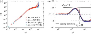
(a) Stress length function shown by DNS data and (b) $Q(y^{+})=\text{d}\ln (\ell _{uv}^{+DNS}/L)/\text{d}\ln (y^{+})$
reveals local scaling in sub-, buffer and log layers with exponents
$Q(y^{+})=\text{d}\ln (\ell _{uv}^{+DNS}/L)/\text{d}\ln (y^{+})$
reveals local scaling in sub-, buffer and log layers with exponents $3/2$
, 2 and 1, respectively. Two channel flows from Iwamoto, Suzuki & Kasagi (Reference Iwamoto, Suzuki and Kasagi2002) at
$3/2$
, 2 and 1, respectively. Two channel flows from Iwamoto, Suzuki & Kasagi (Reference Iwamoto, Suzuki and Kasagi2002) at $Re_{\unicode[STIX]{x1D70F}}=650$
and Hoyas & Jimenez (Reference Hoyas and Jimenez2006) at
$Re_{\unicode[STIX]{x1D70F}}=650$
and Hoyas & Jimenez (Reference Hoyas and Jimenez2006) at $Re_{\unicode[STIX]{x1D70F}}=940$
, one pipe flow of Wu & Moin (Reference Wu and Moin2008) at
$Re_{\unicode[STIX]{x1D70F}}=940$
, one pipe flow of Wu & Moin (Reference Wu and Moin2008) at $Re_{\unicode[STIX]{x1D70F}}=1142$
and one TBL flow of Schlatter et al. (Reference Schlatter, Li, Brethouwer, Johansson and Henningson2010) at
$Re_{\unicode[STIX]{x1D70F}}=1142$
and one TBL flow of Schlatter et al. (Reference Schlatter, Li, Brethouwer, Johansson and Henningson2010) at $Re_{\unicode[STIX]{x1D70F}}=1270$
. Dashed lines indicate sublayer thickness
$Re_{\unicode[STIX]{x1D70F}}=1270$
. Dashed lines indicate sublayer thickness $y_{sub}^{+}=9.7$
and buffer-layer thickness
$y_{sub}^{+}=9.7$
and buffer-layer thickness $y_{buf}^{+}=41$
, respectively, at the middle of scaling transitions.
$y_{buf}^{+}=41$
, respectively, at the middle of scaling transitions.
2.2.1 Ansatz 1: power law
The first ansatz is a constant dilatation invariant for $I_{1}$
, which leads to the power law scaling for the stress length function:
$I_{1}$
, which leads to the power law scaling for the stress length function:
 $$\begin{eqnarray}\text{If }I_{1}=\text{const.},\text{ from }(2.19),\quad \ell =I_{1}y^{\unicode[STIX]{x1D6FC}}.\end{eqnarray}$$
In this case, $I_{2}$
is also a constant, which can be verified by substituting (2.21) into (2.20)
$I_{2}$
is also a constant, which can be verified by substituting (2.21) into (2.20)
 $$\begin{eqnarray}I_{2}=\unicode[STIX]{x1D6FC}I_{1}=\text{const}.\end{eqnarray}$$
The ratio of these two dilatation invariants
 $$\begin{eqnarray}\unicode[STIX]{x1D6FE}=I_{2}/I_{1}=\text{d}\ln (\ell )/\text{d}\ln (\,y)\end{eqnarray}$$
is particularly important because we can use $\unicode[STIX]{x1D6FE}$
as a diagnostic function to analyse DNS data: if there is a power law of
$\unicode[STIX]{x1D6FE}$
as a diagnostic function to analyse DNS data: if there is a power law of $\ell$
in a range of
$\ell$
in a range of $y$
, then
$y$
, then $\unicode[STIX]{x1D6FE}$
displays a local plateau (constant
$\unicode[STIX]{x1D6FE}$
displays a local plateau (constant $\unicode[STIX]{x1D6FC}$
) in the same
$\unicode[STIX]{x1D6FC}$
) in the same $y$
range. How
$y$
range. How $\unicode[STIX]{x1D6FE}$
enables the discovery of different scaling exponents in the viscous sublayer, buffer layer, etc. will be shown later in figure 1.
$\unicode[STIX]{x1D6FE}$
enables the discovery of different scaling exponents in the viscous sublayer, buffer layer, etc. will be shown later in figure 1.
2.2.2 Ansatz 2: defect-power law
When $I_{1}\neq \text{const.}$
, a second invariant relation is postulated:
$I_{1}\neq \text{const.}$
, a second invariant relation is postulated:
 $$\begin{eqnarray}\text{For }I_{1}\neq \text{const}.\text{ but }I_{2}=\text{const}.,\text{ from (2.20)},\quad \text{d}\ell /\text{d}y=I_{2}y^{(\unicode[STIX]{x1D6FC}-1)}.\end{eqnarray}$$
We refer to this case as the dilatation symmetry broken in $\ell$
but preserved in
$\ell$
but preserved in $\text{d}\ell /\text{d}y$
. Integration of (2.24) yields the defect-power law
$\text{d}\ell /\text{d}y$
. Integration of (2.24) yields the defect-power law
 $$\begin{eqnarray}\ell =(I_{2}/\unicode[STIX]{x1D6FC})y^{\unicode[STIX]{x1D6FC}}+c.\end{eqnarray}$$
2.2.3 Ansatz 3: scaling transition, a generalized invariant relation
To describe a smooth and monotonic transition of $\ell$
from one power-law scaling
$\ell$
from one power-law scaling $\ell ^{(I)}=c_{I}y^{\unicode[STIX]{x1D6FE}_{I}}$
to another
$\ell ^{(I)}=c_{I}y^{\unicode[STIX]{x1D6FE}_{I}}$
to another $\ell ^{(II)}=c_{II}y^{\unicode[STIX]{x1D6FE}_{II}}$
(i.e. from one layer to another), a simple transition ansatz can be found with a nonlinear relation between the two dilatation invariants. Specifically, we extend (2.22) to include a nonlinear term (explained below) as
$\ell ^{(II)}=c_{II}y^{\unicode[STIX]{x1D6FE}_{II}}$
(i.e. from one layer to another), a simple transition ansatz can be found with a nonlinear relation between the two dilatation invariants. Specifically, we extend (2.22) to include a nonlinear term (explained below) as
 $$\begin{eqnarray}I_{2}=\unicode[STIX]{x1D6FE}_{I}I_{1}+c\left(I_{1}\right)^{n}\quad \Rightarrow \quad \ell =c_{I}y^{\unicode[STIX]{x1D6FE}_{I}}\left(1+(\,y/y_{c})^{p}\right)^{(\unicode[STIX]{x1D6FE}_{II}-\unicode[STIX]{x1D6FE}_{I})/p},\end{eqnarray}$$
where $I_{1}=\ell /y^{\unicode[STIX]{x1D6FE}_{II}}$
and
$I_{1}=\ell /y^{\unicode[STIX]{x1D6FE}_{II}}$
and $I_{2}=(\text{d}\ell /\text{d}y)/y^{\unicode[STIX]{x1D6FE}_{II}-1}$
. The power laws in the two adjacent layers are
$I_{2}=(\text{d}\ell /\text{d}y)/y^{\unicode[STIX]{x1D6FE}_{II}-1}$
. The power laws in the two adjacent layers are
 $$\begin{eqnarray}\displaystyle & \ell ^{(I)}=c_{I}y^{\unicode[STIX]{x1D6FE}_{I}}\text{ for }y\ll y_{c} & \displaystyle\end{eqnarray}$$
 $$\begin{eqnarray}\displaystyle & \ell ^{(II)}=(c_{I}y_{c}^{\unicode[STIX]{x1D6FE}_{I}-\unicode[STIX]{x1D6FE}_{II}})y^{\unicode[STIX]{x1D6FE}_{II}}\text{ for }y\gg y_{c}, & \displaystyle\end{eqnarray}$$
which are connected at the transition location $y=y_{c}=(c_{I}/c_{II})^{1/(\unicode[STIX]{x1D6FE}_{II}-\unicode[STIX]{x1D6FE}_{I})}$
where
$y=y_{c}=(c_{I}/c_{II})^{1/(\unicode[STIX]{x1D6FE}_{II}-\unicode[STIX]{x1D6FE}_{I})}$
where $\ell ^{(I)}=\ell ^{(II)}$
. Parenthetically, it is interesting that (2.26) has appeared before in some fluid mechanics problems, such as connecting two spectral regions (Batchelor Reference Batchelor1951) and building a compound MVP (L’vov et al.
Reference L’vov, Procaccia and Rudenko2008).
$\ell ^{(I)}=\ell ^{(II)}$
. Parenthetically, it is interesting that (2.26) has appeared before in some fluid mechanics problems, such as connecting two spectral regions (Batchelor Reference Batchelor1951) and building a compound MVP (L’vov et al.
Reference L’vov, Procaccia and Rudenko2008).
The choice of the generalized invariant relation (2.26) is explained below. Note that the left-hand side of (2.26) can be rewritten as $I_{2}/I_{1}=\unicode[STIX]{x1D6FE}_{I}+c\left(I_{1}\right)^{n-1}$
, characterizing the local scaling exponent
$I_{2}/I_{1}=\unicode[STIX]{x1D6FE}_{I}+c\left(I_{1}\right)^{n-1}$
, characterizing the local scaling exponent $\unicode[STIX]{x1D6FE}=I_{2}/I_{1}$
varying from a constant value
$\unicode[STIX]{x1D6FE}=I_{2}/I_{1}$
varying from a constant value $\unicode[STIX]{x1D6FE}_{I}$
(in layer I) to
$\unicode[STIX]{x1D6FE}_{I}$
(in layer I) to $\unicode[STIX]{x1D6FE}_{II}$
(in layer II) by suitable choices of
$\unicode[STIX]{x1D6FE}_{II}$
(in layer II) by suitable choices of $c$
and
$c$
and $n$
. To see this, we rewrite the left-hand side of (2.26) as
$n$
. To see this, we rewrite the left-hand side of (2.26) as
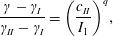 $$\begin{eqnarray}\frac{\unicode[STIX]{x1D6FE}-\unicode[STIX]{x1D6FE}_{I}}{\unicode[STIX]{x1D6FE}_{II}-\unicode[STIX]{x1D6FE}_{I}}=\left(\frac{c_{II}}{I_{1}}\right)^{q},\end{eqnarray}$$
where $n=1-q$
and
$n=1-q$
and $c=(\unicode[STIX]{x1D6FE}_{II}-\unicode[STIX]{x1D6FE}_{I})c_{II}^{q}$
are substituted as compact notations. Then, for
$c=(\unicode[STIX]{x1D6FE}_{II}-\unicode[STIX]{x1D6FE}_{I})c_{II}^{q}$
are substituted as compact notations. Then, for $y\gg y_{c}$
(i.e. approaching layer II),
$y\gg y_{c}$
(i.e. approaching layer II), $I_{1}=\ell /y^{\unicode[STIX]{x1D6FE}_{II}}\rightarrow c_{II}$
, the right-hand side of (2.29) goes to 1, consistent with the left-hand side of (2.29). For
$I_{1}=\ell /y^{\unicode[STIX]{x1D6FE}_{II}}\rightarrow c_{II}$
, the right-hand side of (2.29) goes to 1, consistent with the left-hand side of (2.29). For $y\ll y_{c}$
(approaching layer I), the right-hand side of (2.29) goes to zero when
$y\ll y_{c}$
(approaching layer I), the right-hand side of (2.29) goes to zero when $p=q(\unicode[STIX]{x1D6FE}_{II}-\unicode[STIX]{x1D6FE}_{I})\gg 1$
, consistent with the left-hand side of (2.29). This can always be guaranteed by choosing an appropriate
$p=q(\unicode[STIX]{x1D6FE}_{II}-\unicode[STIX]{x1D6FE}_{I})\gg 1$
, consistent with the left-hand side of (2.29). This can always be guaranteed by choosing an appropriate $q$
where
$q$
where $q$
specifies the sharpness of the transition between the two layers. Therefore, equation (2.29) connecting the two asymptotic power-law states (2.27) and (2.28) is explicitly written as
$q$
specifies the sharpness of the transition between the two layers. Therefore, equation (2.29) connecting the two asymptotic power-law states (2.27) and (2.28) is explicitly written as
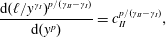 $$\begin{eqnarray}\frac{\text{d}(\ell /y^{\unicode[STIX]{x1D6FE}_{I}})^{p/(\unicode[STIX]{x1D6FE}_{II}-\unicode[STIX]{x1D6FE}_{I})}}{\text{d}(y^{p})}=c_{II}^{p/(\unicode[STIX]{x1D6FE}_{II}-\unicode[STIX]{x1D6FE}_{I})},\end{eqnarray}$$
which, after integration, yields the scaling (simply means power law) transition ansatz, the right-hand side of (2.26),
 $$\begin{eqnarray}\ell =c_{I}y^{\unicode[STIX]{x1D6FE}_{I}}(1+(\,y/y_{c})^{p})^{(\unicode[STIX]{x1D6FE}_{II}-\unicode[STIX]{x1D6FE}_{I})/p}.\end{eqnarray}$$
All of the parameters in (2.31) are determined from (2.29), except for $c_{I}$
which is an integration constant determined by the power-law coefficient in layer I.
$c_{I}$
which is an integration constant determined by the power-law coefficient in layer I.
In the following, we will show that (2.25) and (2.31) serve as the basic analytical structures which, together with the commonly used multiplicative matching rule, define the analytical multi-layer wall function and wake function. Let us emphasise that the functional form of the multi-layer structure is obtained from symmetry analysis, while the parameter values are determined by a variety of other techniques (involving Taylor expansion, heuristic reasoning and empirical data fitting), as presented in the following section.
3 A multi-layer stress length function
The notion of the multi-layer structure in wall turbulence is well known (Pope Reference Pope2000; Wei et al.
Reference Wei, Fife, Klewicki and Mcmurtry2005; Klewicki et al.
Reference Klewicki, Chin, Blackburn, Ooi and Marusic2012). However, our four-layer description below differs from previously defined four layers by Wei et al. (Reference Wei, Fife, Klewicki and Mcmurtry2005) and Klewicki et al. (Reference Klewicki, Chin, Blackburn, Ooi and Marusic2012), who considered the leading-order balance of the mean-momentum equation (viz., layer I extends to $y^{+}\approx 3$
, layer II to
$y^{+}\approx 3$
, layer II to $y^{+}\approx 1.6\sqrt{Re_{\unicode[STIX]{x1D70F}}}$
, layer III to
$y^{+}\approx 1.6\sqrt{Re_{\unicode[STIX]{x1D70F}}}$
, layer III to $y^{+}\approx 2.6\sqrt{Re_{\unicode[STIX]{x1D70F}}}$
and layer IV to the centreline). In the following, we report our Lie-group description of the multi-layer structure of the stress length function and validate the concept using DNS data.
$y^{+}\approx 2.6\sqrt{Re_{\unicode[STIX]{x1D70F}}}$
and layer IV to the centreline). In the following, we report our Lie-group description of the multi-layer structure of the stress length function and validate the concept using DNS data.
First, let us explain two new regions of the flow. According to our study here, a bulk-flow region can be defined by quasi-balance (meaning nearly equal) between production and dissipation. This bulk flow contains the overlap region near the wall and extends to the edge of the TBL; in the case of channel and pipe flows, there is an additional layer, the ‘core layer’, towards the centre, where turbulent transport replaces production with balance dissipation. Below we introduce inner (2.5) and outer scales (2.7) to normalize the stress length function (thereby also balance equations). Specifically, in analogy to the centreline of channel/pipe, an outer dilatation centre is defined for the TBL (let us call it $\unicode[STIX]{x1D6FF}$
, where
$\unicode[STIX]{x1D6FF}$
, where $\unicode[STIX]{x1D6FF}$
is not necessarily
$\unicode[STIX]{x1D6FF}$
is not necessarily $\unicode[STIX]{x1D6FF}_{99}$
commonly used to describe the boundary layer edge of the TBL). The invariant solutions expressed in terms of the stress length function are the same as (2.21), (2.24) and (2.26), but only by replacing
$\unicode[STIX]{x1D6FF}_{99}$
commonly used to describe the boundary layer edge of the TBL). The invariant solutions expressed in terms of the stress length function are the same as (2.21), (2.24) and (2.26), but only by replacing $y$
with
$y$
with $y^{+}$
(inner) or with
$y^{+}$
(inner) or with $r$
(outer). At the end, these postulated solutions should be validated by DNS data, which we present in detail now.
$r$
(outer). At the end, these postulated solutions should be validated by DNS data, which we present in detail now.
3.1 Wall layers
The normalized group invariants for stress length function (2.19) and its derivative (2.20), are respectively
 $$\begin{eqnarray}I_{1}=\ell _{uv}^{+}/y^{+\unicode[STIX]{x1D6FC}},\quad I_{2}=\dot{\ell }_{uv}^{+}/y^{+(\unicode[STIX]{x1D6FC}-1)}.\end{eqnarray}$$
Then, the constant dilatation-invariant assumption in (2.21) yields
 $$\begin{eqnarray}I_{1}=c_{1},\quad \text{and}\quad I_{2}=\unicode[STIX]{x1D6FC}c_{1},\end{eqnarray}$$
which lead to a power-law scaling as a function of $y^{+}$
:
$y^{+}$
:
 $$\begin{eqnarray}\ell _{uv}^{+}=c_{1}y^{+\unicode[STIX]{x1D6FC}}.\end{eqnarray}$$
To test (3.3), we display the following diagnostic function as in (2.23)
 $$\begin{eqnarray}\unicode[STIX]{x1D6FE}=I_{2}/I_{1}=\text{d}\ln (\ell _{uv}^{+})/\text{d}\ln (y^{+}).\end{eqnarray}$$
If the empirical $\unicode[STIX]{x1D6FE}$
as opposed to the theoretical
$\unicode[STIX]{x1D6FE}$
as opposed to the theoretical $\unicode[STIX]{x1D6FC}$
displays a plateau in the range of
$\unicode[STIX]{x1D6FC}$
displays a plateau in the range of $y^{+}$
, then a local power law of
$y^{+}$
, then a local power law of $\ell _{uv}$
is validated and the value of the plateau is thus
$\ell _{uv}$
is validated and the value of the plateau is thus $\unicode[STIX]{x1D6FC}$
. This is shown in figure 1 with
$\unicode[STIX]{x1D6FC}$
. This is shown in figure 1 with $\unicode[STIX]{x1D6FC}=3/2$
in the viscous sublayer,
$\unicode[STIX]{x1D6FC}=3/2$
in the viscous sublayer, $\unicode[STIX]{x1D6FC}=2$
in the buffer layer and
$\unicode[STIX]{x1D6FC}=2$
in the buffer layer and $\unicode[STIX]{x1D6FC}=1$
in the log layer. The scaling in the buffer layer is a typical intermediate asymptotic scaling (Barenblatt Reference Barenblatt1996) covering a restricted domain (
$\unicode[STIX]{x1D6FC}=1$
in the log layer. The scaling in the buffer layer is a typical intermediate asymptotic scaling (Barenblatt Reference Barenblatt1996) covering a restricted domain ( $10\lesssim y^{+}\lesssim 40$
). The calculation of
$10\lesssim y^{+}\lesssim 40$
). The calculation of $\unicode[STIX]{x1D6FE}$
is unavoidably affected by the nearby viscous sublayer and bulk region and the value of scaling exponent 2 appears only at a point (rather than over an extended plateau). Nevertheless, this does not invalidate the concept of the buffer-layer scaling
$\unicode[STIX]{x1D6FE}$
is unavoidably affected by the nearby viscous sublayer and bulk region and the value of scaling exponent 2 appears only at a point (rather than over an extended plateau). Nevertheless, this does not invalidate the concept of the buffer-layer scaling $\ell _{uv}^{+}\propto y^{+2}$
, especially after we employ the third ansatz to form a combined multi-layer description. Also note that in order to present a clear display of
$\ell _{uv}^{+}\propto y^{+2}$
, especially after we employ the third ansatz to form a combined multi-layer description. Also note that in order to present a clear display of $\unicode[STIX]{x1D6FC}=1$
in the log layer, we plot a compensated
$\unicode[STIX]{x1D6FC}=1$
in the log layer, we plot a compensated $\unicode[STIX]{x1D6FE}$
function, i.e.
$\unicode[STIX]{x1D6FE}$
function, i.e. $Q(y^{+})=\text{d}\ln (\ell _{uv}^{+DNS}/L)/\text{d}\ln (y^{+})$
, where
$Q(y^{+})=\text{d}\ln (\ell _{uv}^{+DNS}/L)/\text{d}\ln (y^{+})$
, where $L=\ell _{uv}^{\wedge Outer}/y^{+}$
is the theoretical formula for the outer flow (see later). This compensated plot eliminates the outer-flow influence on the log layer, but without changing the scaling exponents in the viscous sublayer and buffer layer, as
$L=\ell _{uv}^{\wedge Outer}/y^{+}$
is the theoretical formula for the outer flow (see later). This compensated plot eliminates the outer-flow influence on the log layer, but without changing the scaling exponents in the viscous sublayer and buffer layer, as $L$
is a constant near the wall. In the following, we introduce the local power law for each of the layers.
$L$
is a constant near the wall. In the following, we introduce the local power law for each of the layers.
3.1.1 Viscous sublayer
In the viscous sublayer, the stress length function is
 $$\begin{eqnarray}\ell _{uv}^{+sub}=I_{1}^{sub}y^{+3/2}.\end{eqnarray}$$
This can be justified by a near-wall expansion (Pope Reference Pope2000; Wu et al.
Reference Wu, Chen, She and Hussain2012): $u^{\prime }\propto y$
and
$u^{\prime }\propto y$
and $v^{\prime }\propto y^{2}$
such that the Reynolds shear stress
$v^{\prime }\propto y^{2}$
such that the Reynolds shear stress $W^{+}=W/u_{\unicode[STIX]{x1D70F}}^{2}\propto y^{+3}$
. Since
$W^{+}=W/u_{\unicode[STIX]{x1D70F}}^{2}\propto y^{+3}$
. Since $S^{+}\approx 1$
near the wall, thus
$S^{+}\approx 1$
near the wall, thus $\ell _{uv}^{+}\propto y^{+3/2}$
(hence
$\ell _{uv}^{+}\propto y^{+3/2}$
(hence $\unicode[STIX]{x1D6FC}=3/2$
). Note that for
$\unicode[STIX]{x1D6FC}=3/2$
). Note that for $I_{1}^{sub}$
, according to current DNS data, it is approximately 0.034. Interestingly, if we assume
$I_{1}^{sub}$
, according to current DNS data, it is approximately 0.034. Interestingly, if we assume $\ell _{uv}^{+}(\,y_{sub}^{+})\approx 1$
(in wall units), we immediately obtain an estimate of
$\ell _{uv}^{+}(\,y_{sub}^{+})\approx 1$
(in wall units), we immediately obtain an estimate of $y_{sub}^{+}=(I_{1}^{sub})^{-2/3}\approx 9.5$
, which is very close to the final value 9.7 (see figure 1).
$y_{sub}^{+}=(I_{1}^{sub})^{-2/3}\approx 9.5$
, which is very close to the final value 9.7 (see figure 1).
3.1.2 Buffer layer
Note that the log layer is well known as in (1.6), while the viscous sublayer is characterized by (3.5). A natural question is: What is the scaling exponent of the stress length function in the buffer layer? In fact, in the buffer layer, the power law for the stress length function is
 $$\begin{eqnarray}\ell _{uv}^{+buf}=I_{1}^{buf}y^{+2}.\end{eqnarray}$$
A preliminary study yields the following explanation. Using dimensional analysis we obtain $\ell _{uv}=\ell _{\unicode[STIX]{x1D708}}\unicode[STIX]{x1D6E9}^{1/4}$
, where
$\ell _{uv}=\ell _{\unicode[STIX]{x1D708}}\unicode[STIX]{x1D6E9}^{1/4}$
, where $\ell _{\unicode[STIX]{x1D708}}=(W/S)^{3/4}/\unicode[STIX]{x1D700}^{1/4}=\unicode[STIX]{x1D708}_{T}^{3/4}/\unicode[STIX]{x1D700}^{1/4}$
is a shear-induced eddy length and
$\ell _{\unicode[STIX]{x1D708}}=(W/S)^{3/4}/\unicode[STIX]{x1D700}^{1/4}=\unicode[STIX]{x1D708}_{T}^{3/4}/\unicode[STIX]{x1D700}^{1/4}$
is a shear-induced eddy length and $\unicode[STIX]{x1D6E9}=\unicode[STIX]{x1D700}/(SW)$
is the ratio between dissipation and production. A near-wall expansion yields
$\unicode[STIX]{x1D6E9}=\unicode[STIX]{x1D700}/(SW)$
is the ratio between dissipation and production. A near-wall expansion yields $\ell _{\unicode[STIX]{x1D708}}\propto y^{2}$
, while in the buffer layer
$\ell _{\unicode[STIX]{x1D708}}\propto y^{2}$
, while in the buffer layer $\unicode[STIX]{x1D6E9}\approx \text{const.}$
(due to the fact that turbulent transport and dissipation are of the same order as production). Hence,
$\unicode[STIX]{x1D6E9}\approx \text{const.}$
(due to the fact that turbulent transport and dissipation are of the same order as production). Hence, $\ell _{uv}\propto y^{2}$
by multiplying
$\ell _{uv}\propto y^{2}$
by multiplying $\ell _{\unicode[STIX]{x1D708}}$
and
$\ell _{\unicode[STIX]{x1D708}}$
and $\unicode[STIX]{x1D6E9}$
. Such a scaling exponent 2 is shown in figure 1, indicated by a peak in the
$\unicode[STIX]{x1D6E9}$
. Such a scaling exponent 2 is shown in figure 1, indicated by a peak in the $\unicode[STIX]{x1D6FE}$
function located at approximately
$\unicode[STIX]{x1D6FE}$
function located at approximately $y^{+}=20$
; and the coefficient
$y^{+}=20$
; and the coefficient $I_{1}^{buf}\approx 0.01$
from moderate
$I_{1}^{buf}\approx 0.01$
from moderate $Re$
’s DNS data. Whether this power law can be explained by a statistical study of coherent vortex structures (Schoppa & Hussain Reference Schoppa and Hussain2002) in the buffer layer, deserves further study. Interestingly, equation (1.7) assumes also a power-law scaling with exponent 2, but it should be valid in the buffer layer and not the viscous sublayer.
$Re$
’s DNS data. Whether this power law can be explained by a statistical study of coherent vortex structures (Schoppa & Hussain Reference Schoppa and Hussain2002) in the buffer layer, deserves further study. Interestingly, equation (1.7) assumes also a power-law scaling with exponent 2, but it should be valid in the buffer layer and not the viscous sublayer.
3.1.3 Log-law region (log layer)
The power scaling in the log-law region (log layer) is
 $$\begin{eqnarray}\ell _{uv}^{+log}=I_{1}^{log}y^{+}=\unicode[STIX]{x1D705}y^{+},\end{eqnarray}$$
which is the classical assumption made by Prandtl in 1925 (leading to the log law for the mean velocity), i.e. the Karman constant $\unicode[STIX]{x1D705}=I_{1}^{log}$
. Later we will see (3.7) can be obtained from a near-wall asymptotic analysis of a (outer) bulk solution (3.13). Hence, (3.7) is not an assumption.
$\unicode[STIX]{x1D705}=I_{1}^{log}$
. Later we will see (3.7) can be obtained from a near-wall asymptotic analysis of a (outer) bulk solution (3.13). Hence, (3.7) is not an assumption.
3.2 Outer flow
As shown in (2.14), the group invariants for the length function and its derivative are respectively
 $$\begin{eqnarray}I_{1}=\ell _{uv}^{\wedge }/r^{\unicode[STIX]{x1D6FC}},\quad I_{2}=\dot{\ell }_{uv}^{\wedge }/r^{\unicode[STIX]{x1D6FC}-1}\end{eqnarray}$$
and the corresponding diagnostic function for the power-law scaling exponent is
 $$\begin{eqnarray}\unicode[STIX]{x1D6FE}=I_{2}/I_{1}=\unicode[STIX]{x2202}\ln (\ell _{uv}^{\wedge })/\unicode[STIX]{x2202}\ln (r).\end{eqnarray}$$
3.2.1 Core layer
A power law for the stress length can be derived near the centreline (core layer, as $r\rightarrow 0$
)
$r\rightarrow 0$
)
 $$\begin{eqnarray}\ell _{uv}^{\wedge core}=I_{1}^{core}r^{-1/2},\end{eqnarray}$$
which can be explained as follows. The leading-order balance of the mean-momentum equation between the Reynolds stress and the total stress yields $W^{+}\approx \unicode[STIX]{x1D70F}^{+}=r$
; meanwhile, the central symmetry (zero mean shear) yields the first-order expansion
$W^{+}\approx \unicode[STIX]{x1D70F}^{+}=r$
; meanwhile, the central symmetry (zero mean shear) yields the first-order expansion $S^{+}\propto r$
as
$S^{+}\propto r$
as $r\rightarrow 0$
; hence
$r\rightarrow 0$
; hence $\ell _{uv}^{\wedge }=\sqrt{W^{+}}/(Re_{\unicode[STIX]{x1D70F}}S^{+})\propto r^{-1/2}$
, which diverges to infinity as
$\ell _{uv}^{\wedge }=\sqrt{W^{+}}/(Re_{\unicode[STIX]{x1D70F}}S^{+})\propto r^{-1/2}$
, which diverges to infinity as $r\rightarrow 0$
. In a historical context, mixing length is undefined in the core region. Here we resolve this problem by analytically quantifying its asymptotical behaviour and indeed a well-defined formula for it is given and valid in the core. This extra layer is present in a channel/pipe, as shown in figure 2. For the TBL, the core layer is absent, since no centre symmetry is forced by the opposite wall condition (see figure 3). Typical data would show occasional abrupt jumps to the high values of the stress length function outside the boundary layer thickness. Such jumps are obviously artefacts and hence are ignored.
$r\rightarrow 0$
. In a historical context, mixing length is undefined in the core region. Here we resolve this problem by analytically quantifying its asymptotical behaviour and indeed a well-defined formula for it is given and valid in the core. This extra layer is present in a channel/pipe, as shown in figure 2. For the TBL, the core layer is absent, since no centre symmetry is forced by the opposite wall condition (see figure 3). Typical data would show occasional abrupt jumps to the high values of the stress length function outside the boundary layer thickness. Such jumps are obviously artefacts and hence are ignored.
Plot of the stress length function $\ell _{uv}^{+}$
(symbols) divided
$\ell _{uv}^{+}$
(symbols) divided $1-r^{4}$
comparing the current theory with DNS data (Hoyas & Jimenez Reference Hoyas and Jimenez2006). The plateau demonstrates the existence of the bulk flow with the defect-power law (in coordinate
$1-r^{4}$
comparing the current theory with DNS data (Hoyas & Jimenez Reference Hoyas and Jimenez2006). The plateau demonstrates the existence of the bulk flow with the defect-power law (in coordinate $r$
), valid from
$r$
), valid from $y^{+}\approx 50$
to approximately
$y^{+}\approx 50$
to approximately $0.6Re_{\unicode[STIX]{x1D70F}}$
. The lines are composite solutions: the sub-buffer-layer transition
$0.6Re_{\unicode[STIX]{x1D70F}}$
. The lines are composite solutions: the sub-buffer-layer transition $\ell _{uv}^{+(sub\text{-}buf)}$
(compensated by
$\ell _{uv}^{+(sub\text{-}buf)}$
(compensated by $y^{+}$
, solid line), the buffer-log-layer transition
$y^{+}$
, solid line), the buffer-log-layer transition $\ell _{uv}^{+(buf\text{-}log)}$
(compensated by
$\ell _{uv}^{+(buf\text{-}log)}$
(compensated by $y^{+}$
, dashed line) and the bulk-core-layer transition
$y^{+}$
, dashed line) and the bulk-core-layer transition $\ell _{uv}^{+(bulk\text{-}core)}$
(dashed line). See table 1.
$\ell _{uv}^{+(bulk\text{-}core)}$
(dashed line). See table 1.

(a) The stress length function from DNS data (in log–log coordinates) compensated by the bulk-flow formula reveals a four-layer structure, i.e. viscous sublayer, buffer layer, bulk zone and core layer (for channel and pipe), separated by (empirical) layer thicknesses $y_{sub}^{+}\approx 9.7$
,
$y_{sub}^{+}\approx 9.7$
, $y_{buf}^{+}\approx 41$
and
$y_{buf}^{+}\approx 41$
and $r_{core}\approx 0.27$
respectively. (b) The stress length function from DNS data (in log–linear coordinates) shows the constant plateau of the bulk-flow structure, where the green dashed line indicates the bulk-flow constant
$r_{core}\approx 0.27$
respectively. (b) The stress length function from DNS data (in log–linear coordinates) shows the constant plateau of the bulk-flow structure, where the green dashed line indicates the bulk-flow constant $\unicode[STIX]{x1D705}\approx 0.45$
. Note that the stress length profiles in the three flows collapse in the viscous sublayer, buffer layer and bulk flow, by multiplying
$\unicode[STIX]{x1D705}\approx 0.45$
. Note that the stress length profiles in the three flows collapse in the viscous sublayer, buffer layer and bulk flow, by multiplying $m=4$
(channel and TBL) and
$m=4$
(channel and TBL) and $m=5$
(pipe) respectively. Solid lines are theoretical formulas (3.27) and (3.28) with the above parameters (for the TBL, we choose
$m=5$
(pipe) respectively. Solid lines are theoretical formulas (3.27) and (3.28) with the above parameters (for the TBL, we choose $\unicode[STIX]{x1D6FF}=\unicode[STIX]{x1D70E}\unicode[STIX]{x1D6FF}_{99}\approx 0.7\unicode[STIX]{x1D6FF}_{99}$
). Data are the same as in figure 1.
$\unicode[STIX]{x1D6FF}=\unicode[STIX]{x1D70E}\unicode[STIX]{x1D6FF}_{99}\approx 0.7\unicode[STIX]{x1D6FF}_{99}$
). Data are the same as in figure 1.
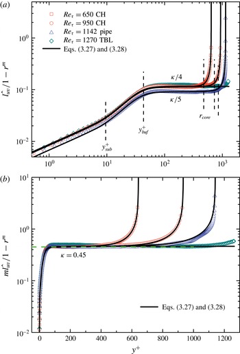
3.2.2 Bulk flow (quasi-balance region)
The bulk flow is defined by a quasi-balance between production (SW) and dissipation ( $\unicode[STIX]{x1D700}$
). In this region,
$\unicode[STIX]{x1D700}$
). In this region, $\unicode[STIX]{x1D6E9}=\unicode[STIX]{x1D700}/(SW)\approx 1$
and
$\unicode[STIX]{x1D6E9}=\unicode[STIX]{x1D700}/(SW)\approx 1$
and $\ell _{\unicode[STIX]{x1D708}}=\unicode[STIX]{x1D708}_{T}^{3/4}/\unicode[STIX]{x1D700}^{1/4}\rightarrow \ell _{e}$
as
$\ell _{\unicode[STIX]{x1D708}}=\unicode[STIX]{x1D708}_{T}^{3/4}/\unicode[STIX]{x1D700}^{1/4}\rightarrow \ell _{e}$
as $r\rightarrow 0$
(finite dissipation and eddy viscosity), therefore
$r\rightarrow 0$
(finite dissipation and eddy viscosity), therefore $\ell _{uv}=\ell _{\unicode[STIX]{x1D708}}\unicode[STIX]{x1D6E9}^{1/4}\approx \ell _{\unicode[STIX]{x1D708}}\rightarrow \ell _{e}$
(Chen, Hussain & She Reference Chen, Hussain and She2016b
). The existence of a finite
$\ell _{uv}=\ell _{\unicode[STIX]{x1D708}}\unicode[STIX]{x1D6E9}^{1/4}\approx \ell _{\unicode[STIX]{x1D708}}\rightarrow \ell _{e}$
(Chen, Hussain & She Reference Chen, Hussain and She2016b
). The existence of a finite $\ell _{e}$
introduces a characteristic length, which contradicts the dilatation symmetry of
$\ell _{e}$
introduces a characteristic length, which contradicts the dilatation symmetry of $\ell _{uv}$
generally implying the absence of any characteristic length. In this case, we need to skip the constant
$\ell _{uv}$
generally implying the absence of any characteristic length. In this case, we need to skip the constant $I_{1}$
assumption, but assume a constant group invariant for its first derivative only, i.e.
$I_{1}$
assumption, but assume a constant group invariant for its first derivative only, i.e.
 $$\begin{eqnarray}I_{1}\neq \text{const}.\quad \text{and}\quad I_{2}=\text{const}.\end{eqnarray}$$
Once again, when the dilatation symmetry in the length function itself is broken, it may still be preserved for its derivative. Integrating (3.11) using (3.8) yields
 $$\begin{eqnarray}\ell _{uv}^{\wedge }=(I_{2}/m)r^{m}+c,\end{eqnarray}$$
where $c$
is an integration constant and
$c$
is an integration constant and $m$
(
$m$
( $=\unicode[STIX]{x1D6FC}$
) is a scaling exponent.
$=\unicode[STIX]{x1D6FC}$
) is a scaling exponent.
Note that (3.12) should be consistent with the wall condition $\ell _{uv}^{\wedge }\rightarrow 0$
as
$\ell _{uv}^{\wedge }\rightarrow 0$
as $r\rightarrow 1$
(towards the wall), then
$r\rightarrow 1$
(towards the wall), then $c=-I_{2}/m$
. A consequence is that we obtain a linear asymptotic scaling for
$c=-I_{2}/m$
. A consequence is that we obtain a linear asymptotic scaling for $\ell _{uv}^{\wedge }$
as
$\ell _{uv}^{\wedge }$
as $r\rightarrow 1$
, i.e.
$r\rightarrow 1$
, i.e. $\ell _{uv}^{\wedge }\rightarrow -I_{2}(1-r)=-I_{2}(\,y/\unicode[STIX]{x1D6FF})$
, which is, in viscous units,
$\ell _{uv}^{\wedge }\rightarrow -I_{2}(1-r)=-I_{2}(\,y/\unicode[STIX]{x1D6FF})$
, which is, in viscous units, $\ell _{uv}^{+}\rightarrow -I_{2}y^{+}$
. This is exactly the linear scaling (3.7) in the log layer. By defining
$\ell _{uv}^{+}\rightarrow -I_{2}y^{+}$
. This is exactly the linear scaling (3.7) in the log layer. By defining $\unicode[STIX]{x1D705}=-I_{2}$
, (3.12) is exactly (3.7) when
$\unicode[STIX]{x1D705}=-I_{2}$
, (3.12) is exactly (3.7) when $r\rightarrow 1$
. Therefore, the final expression for the bulk flow is
$r\rightarrow 1$
. Therefore, the final expression for the bulk flow is
 $$\begin{eqnarray}\ell _{uv}^{\wedge bulk}=\unicode[STIX]{x1D705}(1-r^{m})/m,\end{eqnarray}$$
and the Karman constant is in fact the dilatation-group invariant of the bulk flow. As long as the dilatation symmetry holds, $\unicode[STIX]{x1D705}$
is a constant. This is a very interesting finding as the constancy of
$\unicode[STIX]{x1D705}$
is a constant. This is a very interesting finding as the constancy of $\unicode[STIX]{x1D705}$
has been the subject of numerous controversies in the literature (Nagib & Chauhan Reference Nagib and Chauhan2008; Marusic et al.
Reference Marusic, McKeon, Monkewitz, Nagib, Smits and Sreenivasan2010), although we have asserted a universal
$\unicode[STIX]{x1D705}$
has been the subject of numerous controversies in the literature (Nagib & Chauhan Reference Nagib and Chauhan2008; Marusic et al.
Reference Marusic, McKeon, Monkewitz, Nagib, Smits and Sreenivasan2010), although we have asserted a universal $\unicode[STIX]{x1D705}$
(Chen, Hussain & She Reference Chen, Hussain and She2016a
; Chen et al.
Reference Chen, Hussain and She2016b
; Chen & She Reference Chen and She2016). This new interpretation also implies that
$\unicode[STIX]{x1D705}$
(Chen, Hussain & She Reference Chen, Hussain and She2016a
; Chen et al.
Reference Chen, Hussain and She2016b
; Chen & She Reference Chen and She2016). This new interpretation also implies that $\unicode[STIX]{x1D705}$
can be measured from the bulk-flow data hence can be free of the ambiguity of the non-unique overlap region. Moreover, a theoretical determination the scaling exponent
$\unicode[STIX]{x1D705}$
can be measured from the bulk-flow data hence can be free of the ambiguity of the non-unique overlap region. Moreover, a theoretical determination the scaling exponent $m$
was reported by Chen et al. (Reference Chen, Hussain and She2016b
), where a variational argument yields
$m$
was reported by Chen et al. (Reference Chen, Hussain and She2016b
), where a variational argument yields $m=4$
for the flat wall (channel and TBL) and
$m=4$
for the flat wall (channel and TBL) and $m=5$
for the cylindrical wall (pipe).
$m=5$
for the cylindrical wall (pipe).
3.3 Scaling transition between adjacent layers
The above results give a (local) quantitative characterization of the multi-layer structure, i.e. power laws for viscous sublayer, buffer layer and core layer, and defect-power law for bulk flow. As proposed by Oberlack & Rosteck (Reference Oberlack and Rosteck2010), it is an open issue to describe scaling matching between different layers, which is now addressed by using the generalized invariant relation (2.26) (or (2.29)) as below.
Applying (2.29) to the viscous sublayer and buffer layer yields
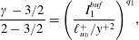 $$\begin{eqnarray}\frac{\unicode[STIX]{x1D6FE}-3/2}{2-3/2}=\left(\frac{I_{1}^{buf}}{\ell _{uv}^{+}/y^{+2}}\right)^{q_{1}},\end{eqnarray}$$
where $3/2$
and 2 are the scaling exponents in the sublayer and buffer layer, respectively; and
$3/2$
and 2 are the scaling exponents in the sublayer and buffer layer, respectively; and $I_{1}^{buf}$
is the constant dilatation invariant in the buffer layer. It leads to the following scaling transition function connecting the two layers, (3.5) and (3.6), together as follows:
$I_{1}^{buf}$
is the constant dilatation invariant in the buffer layer. It leads to the following scaling transition function connecting the two layers, (3.5) and (3.6), together as follows:
 $$\begin{eqnarray}\ell _{uv}^{+(sub\text{-}buf)}=I_{1}^{sub}y^{+3/2}\left(1+\left(\frac{y^{+}}{y_{sub}^{+}}\right)^{p_{1}}\right)^{1/2p_{1}}=\ell _{0}\left(\frac{y^{+}}{y_{sub}^{+}}\right)^{3/2}\left(1+\left(\frac{y^{+}}{y_{sub}^{+}}\right)^{p_{1}}\right)^{1/2p_{1}},\end{eqnarray}$$
where the constant dilatation invariants $I_{1}^{sub}$
and
$I_{1}^{sub}$
and $I_{1}^{buf}$
are replaced by
$I_{1}^{buf}$
are replaced by $y_{sub}^{+}=(I_{1}^{sub}/I_{1}^{buf})^{2}$
(which is called the sublayer thickness and takes a value of approximately 9.7 shown in figure 1) and
$y_{sub}^{+}=(I_{1}^{sub}/I_{1}^{buf})^{2}$
(which is called the sublayer thickness and takes a value of approximately 9.7 shown in figure 1) and $\ell _{0}=I_{1}^{sub}(I_{1}^{sub}/I_{1}^{buf})^{3}\approx 1.03$
(determined from
$\ell _{0}=I_{1}^{sub}(I_{1}^{sub}/I_{1}^{buf})^{3}\approx 1.03$
(determined from $\unicode[STIX]{x1D705}$
). Note also that the transition sharpness
$\unicode[STIX]{x1D705}$
). Note also that the transition sharpness $p_{1}=q_{1}(2-3/2)=q_{1}/2$
is set as integer 4, which is least sensitive to predict MVP.
$p_{1}=q_{1}(2-3/2)=q_{1}/2$
is set as integer 4, which is least sensitive to predict MVP.
Similarly, for buffer and log layers, by using (2.29)
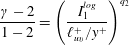 $$\begin{eqnarray}\frac{\unicode[STIX]{x1D6FE}-2}{1-2}=\left(\frac{I_{1}^{log}}{\ell _{uv}^{+}/y^{+}}\right)^{q_{2}}\end{eqnarray}$$
one has the following scaling transition:
 $$\begin{eqnarray}\ell _{uv}^{+(buf\text{-}log)}=I_{1}^{buf}y_{}^{+2}\left(1+\left(\frac{y^{+}}{y_{buf}^{+}}\right)^{p_{2}}\right)^{-1/p_{2}}=\ell _{0}\left(\frac{y^{+}}{y_{sub}^{+}}\right)^{2}\left(1+\left(\frac{y^{+}}{y_{buf}^{+}}\right)^{p_{2}}\right)^{-1/p_{2}},\end{eqnarray}$$
where $y_{buf}^{+}=I_{1}^{log}/I_{1}^{buf}=\unicode[STIX]{x1D705}y_{sub}^{+2}/\ell _{0}$
(approximately 41, as shown in figure 1); and
$y_{buf}^{+}=I_{1}^{log}/I_{1}^{buf}=\unicode[STIX]{x1D705}y_{sub}^{+2}/\ell _{0}$
(approximately 41, as shown in figure 1); and $p_{2}=4$
, the same as
$p_{2}=4$
, the same as $p_{1}$
.
$p_{1}$
.
The generalized invariant relation also works accurately for the outer flow. Note that the bulk solution (3.13) saturates to a constant $\ell _{uv}^{\wedge }\rightarrow \unicode[STIX]{x1D705}/m$
towards the centre, indicating a zero scaling exponent, while the scaling exponent in the core layer is
$\ell _{uv}^{\wedge }\rightarrow \unicode[STIX]{x1D705}/m$
towards the centre, indicating a zero scaling exponent, while the scaling exponent in the core layer is $-1/2$
; thus applying (2.29) to the bulk edge and the core-layer yields
$-1/2$
; thus applying (2.29) to the bulk edge and the core-layer yields
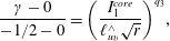 $$\begin{eqnarray}\frac{\unicode[STIX]{x1D6FE}-0}{-1/2-0}=\left(\frac{I_{1}^{core}}{\ell _{uv}^{\wedge }\sqrt{r}}\right)^{q_{3}},\end{eqnarray}$$
where $\unicode[STIX]{x1D6FE}$
is a function of
$\unicode[STIX]{x1D6FE}$
is a function of $r$
as in (3.9). Integrating (3.18) with respect to
$r$
as in (3.9). Integrating (3.18) with respect to $r$
leads to the following composite solution:
$r$
leads to the following composite solution:
 $$\begin{eqnarray}\ell _{uv}^{\wedge (bulk\text{-}core)}=(\unicode[STIX]{x1D705}/m)(1+(r/r_{core})^{p_{3}})^{-1/(2p_{3})}/Z_{c},\end{eqnarray}$$
where $Z_{c}=(1+(1/r_{core})^{p_{3}})^{-1/(2p_{3})}$
obtained from
$Z_{c}=(1+(1/r_{core})^{p_{3}})^{-1/(2p_{3})}$
obtained from $\ell _{uv}^{\wedge }\rightarrow \unicode[STIX]{x1D705}/m$
as
$\ell _{uv}^{\wedge }\rightarrow \unicode[STIX]{x1D705}/m$
as $r\rightarrow 1$
, and
$r\rightarrow 1$
, and $I_{1}^{core}=(\unicode[STIX]{x1D705}r_{core}^{1/2})/(mZ_{c})$
is replaced by the core layer thickness
$I_{1}^{core}=(\unicode[STIX]{x1D705}r_{core}^{1/2})/(mZ_{c})$
is replaced by the core layer thickness $r_{core}$
(which is then measured to be 0.27 shown later). Note that the sharpness
$r_{core}$
(which is then measured to be 0.27 shown later). Note that the sharpness $p_{3}$
has been derived by us (Chen et al.
Reference Chen, Hussain and She2016b
) to be
$p_{3}$
has been derived by us (Chen et al.
Reference Chen, Hussain and She2016b
) to be $-2$
from a central symmetry consideration, which is summarized as follows. From (3.19), we can calculate that near the centreline
$-2$
from a central symmetry consideration, which is summarized as follows. From (3.19), we can calculate that near the centreline $\unicode[STIX]{x2202}_{r}\unicode[STIX]{x1D700}\propto r^{-p_{3}-1}$
(using
$\unicode[STIX]{x2202}_{r}\unicode[STIX]{x1D700}\propto r^{-p_{3}-1}$
(using $\unicode[STIX]{x1D700}=SW\unicode[STIX]{x1D6E9}$
). On the other hand, the dissipation is parabolic in the core layer (as
$\unicode[STIX]{x1D700}=SW\unicode[STIX]{x1D6E9}$
). On the other hand, the dissipation is parabolic in the core layer (as $\unicode[STIX]{x2202}_{r}\unicode[STIX]{x1D700}=0$
at the centre). Thus, by requiring equality between our calculation and the symmetry consideration, i.e.
$\unicode[STIX]{x2202}_{r}\unicode[STIX]{x1D700}=0$
at the centre). Thus, by requiring equality between our calculation and the symmetry consideration, i.e. $\unicode[STIX]{x2202}_{r}\unicode[STIX]{x1D700}\propto r^{-p_{3}-1}\propto r$
, one has
$\unicode[STIX]{x2202}_{r}\unicode[STIX]{x1D700}\propto r^{-p_{3}-1}\propto r$
, one has $p_{3}=-2$
.
$p_{3}=-2$
.
The multi-layer representations of the invariant solutions are summarized in table 1. Note that the defect-power law in the quasi-balance region connects two asymptotic scalings, i.e. linear scaling in the log layer and the finite constant value at the bulk edge. Figure 2 displays clear robust scaling, confirming the existence of dilatation invariance in each layer. One may wonder why the invariance (symmetry) is preserved in each layer. It is a conjecture that turbulence preserves statistical symmetries (Frisch Reference Frisch1995) (which means symmetry on the statistical quantities). Here, the dilatation symmetry is indeed preserved locally in the stress length hence validating that conjecture. The dilatation invariance in both the viscous sublayer and the central core layer can be rigorously proven using the boundary constraints. New dilatation invariance suggested by us includes the power law (e.g. $y^{+2}$
) in the buffer layer and the defect-power law (e.g.
$y^{+2}$
) in the buffer layer and the defect-power law (e.g. $1-r^{m}$
) in the bulk flow. In conclusion, while prior approaches have applied dilatation invariance to the MVP, our approach pushes the level higher by applying dilatation invariance to a turbulence quantity, namely stress length function.
$1-r^{m}$
) in the bulk flow. In conclusion, while prior approaches have applied dilatation invariance to the MVP, our approach pushes the level higher by applying dilatation invariance to a turbulence quantity, namely stress length function.
Multi-layer structure for the stress length function. The first layer adjacent to the wall is the viscous sublayer ending at $y_{sub}^{+}\approx 9.7$
; then it is the buffer layer ending at
$y_{sub}^{+}\approx 9.7$
; then it is the buffer layer ending at $y_{buf}^{+}\approx 41$
; the core layer extends from the centreline to the core layer thickness
$y_{buf}^{+}\approx 41$
; the core layer extends from the centreline to the core layer thickness $r_{core}\approx 0.27$
and the remaining flow domain is the bulk-flow region. The right column shows the scaling transition which connects local power laws in adjacent layers (middle column) together. Note that
$r_{core}\approx 0.27$
and the remaining flow domain is the bulk-flow region. The right column shows the scaling transition which connects local power laws in adjacent layers (middle column) together. Note that $m=4$
for channel and the TBL,
$m=4$
for channel and the TBL, $m=5$
for pipe, and
$m=5$
for pipe, and $\ell _{0}=\unicode[STIX]{x1D705}y_{sub}^{+2}/y_{buf}^{+}$
,
$\ell _{0}=\unicode[STIX]{x1D705}y_{sub}^{+2}/y_{buf}^{+}$
, $Z_{c}=(1+r_{core}^{2})^{1/4}$
.
$Z_{c}=(1+r_{core}^{2})^{1/4}$
.

3.4 Composite stress length function for the entire flow
To obtain a composite formula for the entire flow domain, we use the following multiplicative rule (Van Dyke Reference Van Dyke1964):
 $$\begin{eqnarray}\unicode[STIX]{x1D719}^{I\text{-}III}=\unicode[STIX]{x1D719}^{I\text{-}II}\unicode[STIX]{x1D719}^{II\text{-}III}/\unicode[STIX]{x1D719}^{Common}.\end{eqnarray}$$
Note that for the inner three layers, the multiplicative rule corresponds to
 $$\begin{eqnarray}\ell _{uv}^{+In}=\ell _{uv}^{+(sub\text{-}buf)}\ell _{uv}^{+(buf\text{-}log)}/\ell _{uv}^{+buf},\end{eqnarray}$$
which leads to the following composite solution for the inner flow
 $$\begin{eqnarray}\ell _{uv}^{+In}=\ell _{0}\left(\frac{y^{+}}{y_{sub}^{+}}\right)^{3/2}\left(1+\left(\frac{y^{+}}{y_{sub}^{+}}\right)^{4}\right)^{1/8}\left(1+\left(\frac{y^{+}}{y_{buf}^{+}}\right)^{4}\right)^{-1/4}.\end{eqnarray}$$
Similarly, applying the multiplicative rule to the outer flow
 $$\begin{eqnarray}\ell _{uv}^{\wedge Outer}=\ell _{uv}^{\wedge bulk}\ell _{uv}^{\wedge (bulk\text{-}core)}/\ell _{0}^{\wedge },\end{eqnarray}$$
where $\ell _{0}^{\wedge }=\unicode[STIX]{x1D705}/m$
, the resulting outer solution is
$\ell _{0}^{\wedge }=\unicode[STIX]{x1D705}/m$
, the resulting outer solution is
 $$\begin{eqnarray}\displaystyle \text{CH }\& \text{ Pipe} & : & \displaystyle \ell _{uv}^{\wedge Outer}=\frac{\unicode[STIX]{x1D705}}{mZ_{c}}(1-r^{m})\left(1+\left(\frac{r_{core}}{r}\right)^{2}\right)^{1/4};\end{eqnarray}$$
 $$\begin{eqnarray}\displaystyle \text{TBL} & : & \displaystyle \ell _{uv}^{\wedge Outer}=\frac{\unicode[STIX]{x1D705}}{4}(1-r^{4}).\end{eqnarray}$$
Finally, the composite stress length for the entire flow domain is obtained by
 $$\begin{eqnarray}\ell _{uv}^{+}=\ell _{uv}^{+In}\ell _{uv}^{+Outer}/\ell _{uv}^{+Common}=\ell _{uv}^{+In}\ell _{uv}^{+Outer}/\ell _{uv}^{+log},\end{eqnarray}$$
which is (for channel and pipe)
 $$\begin{eqnarray}\ell _{uv}^{+}=\ell _{0}\left(\frac{y^{+}}{y_{sub}^{+}}\right)^{3/2}\!\left(1+\left(\frac{y^{+}}{y_{sub}^{+}}\right)^{4}\right)^{\!1/8}\left(1+\left(\frac{y^{+}}{y_{buf}^{+}}\right)^{4}\right)^{\!-1/4}\frac{1-r^{m}}{m(1-r)Z_{c}}\left(1+\left(\frac{r_{core}}{r}\right)^{2}\right)^{\!1/4}.\end{eqnarray}$$
For the TBL, the entire formula is the same, except for the absence of the core layer
 $$\begin{eqnarray}\ell _{uv}^{+}=\ell _{0}\left(\frac{y^{+}}{y_{sub}^{+}}\right)^{3/2}\left(1+\left(\frac{y^{+}}{y_{sub}^{+}}\right)^{4}\right)^{1/8}\left(1+\left(\frac{y^{+}}{y_{buf}^{+}}\right)^{4}\right)^{-1/4}\frac{1-r^{4}}{4(1-r)}.\end{eqnarray}$$
Figures 2 and 3 show verifications of (3.27) and (3.28) compensated by the bulk-flow structure, $1-r^{m}$
, where the agreement with DNS data is quite satisfactory. Note that each of the inner layers and the core (divergent) layer are demarcated by the corresponding layer thicknesses.
$1-r^{m}$
, where the agreement with DNS data is quite satisfactory. Note that each of the inner layers and the core (divergent) layer are demarcated by the corresponding layer thicknesses.
4 Validation of wall function and wake function
4.1 Validation by DNS data for moderate $Re$
$Re$

As in the preceding introduction, in the near-wall region ( $y/\unicode[STIX]{x1D6FF}\rightarrow 0$
),
$y/\unicode[STIX]{x1D6FF}\rightarrow 0$
), $\unicode[STIX]{x1D6F7}(y/\unicode[STIX]{x1D6FF},y/\unicode[STIX]{x1D6FF}_{\unicode[STIX]{x1D708}})\rightarrow \unicode[STIX]{x1D6F7}_{1}(0,y/\unicode[STIX]{x1D6FF}_{\unicode[STIX]{x1D708}})=f_{w}(y^{+})$
, which is called the wall function. It is believed to be universal for canonical wall-bounded flows (Pope Reference Pope2000); this concept has been widely used in numerical modelling of wall flows, when the grid resolution becomes problematic. A well-known wall function is the van Driest (Reference Driest1956) damping function (1.9), which bears an incorrect asymptotic scaling
$\unicode[STIX]{x1D6F7}(y/\unicode[STIX]{x1D6FF},y/\unicode[STIX]{x1D6FF}_{\unicode[STIX]{x1D708}})\rightarrow \unicode[STIX]{x1D6F7}_{1}(0,y/\unicode[STIX]{x1D6FF}_{\unicode[STIX]{x1D708}})=f_{w}(y^{+})$
, which is called the wall function. It is believed to be universal for canonical wall-bounded flows (Pope Reference Pope2000); this concept has been widely used in numerical modelling of wall flows, when the grid resolution becomes problematic. A well-known wall function is the van Driest (Reference Driest1956) damping function (1.9), which bears an incorrect asymptotic scaling $\ell _{uv}\propto y^{2}$
in the viscous sublayer that should be
$\ell _{uv}\propto y^{2}$
in the viscous sublayer that should be $\ell _{uv}\propto y^{3/2}$
, as in (3.5).
$\ell _{uv}\propto y^{3/2}$
, as in (3.5).
Here, we propose a further improvement to the wall function. Substituting $\ell _{uv}^{+}$
into the momentum balance equation, which is
$\ell _{uv}^{+}$
into the momentum balance equation, which is $S^{+}+W^{+}=\unicode[STIX]{x1D70F}^{+}$
in common with channel, pipe and TBL flows (Pope Reference Pope2000), the solution for the mean shear for three flows can be generally denoted as
$S^{+}+W^{+}=\unicode[STIX]{x1D70F}^{+}$
in common with channel, pipe and TBL flows (Pope Reference Pope2000), the solution for the mean shear for three flows can be generally denoted as
 $$\begin{eqnarray}\displaystyle & \displaystyle S^{+}=\left.\left(-1+\sqrt{1+4\unicode[STIX]{x1D70F}^{+}\ell _{uv}^{+2}}\right)\right/(2\ell _{uv}^{+2}), & \displaystyle\end{eqnarray}$$
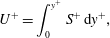 $$\begin{eqnarray}\displaystyle & \displaystyle U^{+}=\int _{0}^{y^{+}}S^{+}\,\text{d}y^{+}, & \displaystyle\end{eqnarray}$$
where $\unicode[STIX]{x1D70F}^{+}$
is the total stress. For channel and pipe flows,
$\unicode[STIX]{x1D70F}^{+}$
is the total stress. For channel and pipe flows, $\unicode[STIX]{x1D70F}^{+}=1-y^{+}/Re_{\unicode[STIX]{x1D70F}}$
exactly; for the TBL,
$\unicode[STIX]{x1D70F}^{+}=1-y^{+}/Re_{\unicode[STIX]{x1D70F}}$
exactly; for the TBL, $\unicode[STIX]{x1D70F}^{+}$
can be derived from the wall normal velocity using the NS equation, which is
$\unicode[STIX]{x1D70F}^{+}$
can be derived from the wall normal velocity using the NS equation, which is $\unicode[STIX]{x1D70F}^{+}=1+\int _{0}^{y}(U^{+}\unicode[STIX]{x2202}_{x}U^{+}+V^{+}\unicode[STIX]{x2202}_{y^{\prime }}U^{+})\,\text{d}y^{\prime }$
. Commonly, all three flows have
$\unicode[STIX]{x1D70F}^{+}=1+\int _{0}^{y}(U^{+}\unicode[STIX]{x2202}_{x}U^{+}+V^{+}\unicode[STIX]{x2202}_{y^{\prime }}U^{+})\,\text{d}y^{\prime }$
. Commonly, all three flows have $\unicode[STIX]{x1D70F}^{+}\approx 1$
in the near-wall region. Substituting
$\unicode[STIX]{x1D70F}^{+}\approx 1$
in the near-wall region. Substituting $\unicode[STIX]{x1D70F}^{+}=1$
into (4.1) and (4.2), one has respectively
$\unicode[STIX]{x1D70F}^{+}=1$
into (4.1) and (4.2), one has respectively
 $$\begin{eqnarray}\displaystyle & \displaystyle S^{+}(\,y^{+})=\left.\left(-1+\sqrt{1+4\ell _{uv}^{+2}}\right)\right/(2\ell _{uv}^{+2}), & \displaystyle\end{eqnarray}$$
 $$\begin{eqnarray}\displaystyle & \displaystyle U^{+}(\,y^{+})=\int _{0}^{y^{+}}\left.\left(-1+\sqrt{1+4\ell _{uv}^{+2}}\right)\right/(2\ell _{uv}^{+2})\,\text{d}y^{+}, & \displaystyle\end{eqnarray}$$
where $\ell _{uv}^{+}$
for the near-wall region is given in (3.22)
$\ell _{uv}^{+}$
for the near-wall region is given in (3.22)
 $$\begin{eqnarray}\displaystyle \ell _{uv}^{+}=\ell _{0}\left(\frac{y^{+}}{y_{sub}^{+}}\right)^{3/2}\left(1+\left(\frac{y^{+}}{y_{sub}^{+}}\right)^{4}\right)^{1/8}\left(1+\left(\frac{y^{+}}{y_{buf}^{+}}\right)^{4}\right)^{-1/4}. & & \displaystyle\end{eqnarray}$$
With the empirical parameters $y_{sub}^{+}=9.7$
,
$y_{sub}^{+}=9.7$
, $\unicode[STIX]{x1D705}=0.45$
and
$\unicode[STIX]{x1D705}=0.45$
and $y_{buf}^{+}=41$
(while
$y_{buf}^{+}=41$
(while $\ell _{0}=\unicode[STIX]{x1D705}y_{sub}^{+2}/y_{buf}^{+}\approx 1.03$
), the resulting MVPs are plotted in figure 4 and the agreement with data is good from the wall up to
$\ell _{0}=\unicode[STIX]{x1D705}y_{sub}^{+2}/y_{buf}^{+}\approx 1.03$
), the resulting MVPs are plotted in figure 4 and the agreement with data is good from the wall up to $y^{+}\approx 300$
. This supports a universal wall function for channel, pipe and TBL flows. In fact, our preliminary study also shows that the new wall function (4.4) with (4.5) applies to compressible channel, pipe and TBL flows, as well as to TBL flows with pressure gradient effects. This establishes the universal multi-layer formula of stress length.
$y^{+}\approx 300$
. This supports a universal wall function for channel, pipe and TBL flows. In fact, our preliminary study also shows that the new wall function (4.4) with (4.5) applies to compressible channel, pipe and TBL flows, as well as to TBL flows with pressure gradient effects. This establishes the universal multi-layer formula of stress length.

Note that the outer-flow prediction of MVP can be given through the integration of $S^{+}\approx \sqrt{\unicode[STIX]{x1D70F}^{+}}/\ell _{uv}^{+}$
. Taking channel and pipe flows for example,
$S^{+}\approx \sqrt{\unicode[STIX]{x1D70F}^{+}}/\ell _{uv}^{+}$
. Taking channel and pipe flows for example, $\unicode[STIX]{x1D70F}^{+}=1-y^{+}/Re_{\unicode[STIX]{x1D70F}}=r$
(the TBL is treated in Chen & She Reference Chen and She2016), and the stress length function is given in (3.24). Thus,
$\unicode[STIX]{x1D70F}^{+}=1-y^{+}/Re_{\unicode[STIX]{x1D70F}}=r$
(the TBL is treated in Chen & She Reference Chen and She2016), and the stress length function is given in (3.24). Thus,
 $$\begin{eqnarray}U^{+}=U_{c}^{+}-\int _{0}^{r}\frac{\sqrt{r^{\prime }}}{\ell _{uv}^{\wedge Outer}}\,\text{d}r^{\prime }=U_{c}^{+}-\int _{0}^{r}\frac{mr^{\prime }[(1+{r_{core}}^{2})/({r^{\prime }}^{2}+{r_{core}}^{2})]^{1/4}}{\unicode[STIX]{x1D705}(1-{r^{\prime }}^{m})}\,\text{d}r^{\prime },\end{eqnarray}$$
where $\unicode[STIX]{x1D705}$
and
$\unicode[STIX]{x1D705}$
and $r_{core}$
are measured as follows. A direct way to measure
$r_{core}$
are measured as follows. A direct way to measure $\unicode[STIX]{x1D705}$
is to examine the compensated stress length function, i.e.
$\unicode[STIX]{x1D705}$
is to examine the compensated stress length function, i.e. $m\ell _{uv}^{\wedge }/(1-r^{m})$
, as shown in figure 3(b) where a plateau identifies the bulk zone and yields an estimate of
$m\ell _{uv}^{\wedge }/(1-r^{m})$
, as shown in figure 3(b) where a plateau identifies the bulk zone and yields an estimate of $\unicode[STIX]{x1D705}\approx 0.45$
. However, this method requires high-quality Reynolds-shear-stress and mean-shear data, and avoiding the influence of data noise. We develop an integration method to measure
$\unicode[STIX]{x1D705}\approx 0.45$
. However, this method requires high-quality Reynolds-shear-stress and mean-shear data, and avoiding the influence of data noise. We develop an integration method to measure $\unicode[STIX]{x1D705}$
and
$\unicode[STIX]{x1D705}$
and $r_{core}$
, based on the MVP data as input.
$r_{core}$
, based on the MVP data as input.
We rewrite (4.6) as
 $$\begin{eqnarray}U^{+}(r)=U_{c}^{+}-\frac{1}{\unicode[STIX]{x1D705}}f(r;r_{core}),\end{eqnarray}$$
where $f$
is
$f$
is
 $$\begin{eqnarray}f(r;r_{core})=m(1+r_{core}^{2})^{1/4}\int _{0}^{r}r^{\prime }/[(1-{r^{\prime }}^{m})({r^{\prime }}^{2}+r_{core}^{2})^{1/4}]\,\text{d}r^{\prime },\end{eqnarray}$$
( $m=4$
for channel and 5 for pipe). Then, the integration method consists of minimising the errors between the theoretical prediction of (4.7) and empirical MVP data for varying
$m=4$
for channel and 5 for pipe). Then, the integration method consists of minimising the errors between the theoretical prediction of (4.7) and empirical MVP data for varying $\unicode[STIX]{x1D705}$
and
$\unicode[STIX]{x1D705}$
and $r_{core}$
. This can also be considered as a fitting procedure with two parameters as follows. Let
$r_{core}$
. This can also be considered as a fitting procedure with two parameters as follows. Let $U^{+Em}(r_{i})$
be a set of empirically measured mean velocities. Denote the theoretical mean velocity from (4.7) as
$U^{+Em}(r_{i})$
be a set of empirically measured mean velocities. Denote the theoretical mean velocity from (4.7) as $U^{+The}(r_{i};\unicode[STIX]{x1D705},r_{core})$
with corresponding parameters
$U^{+The}(r_{i};\unicode[STIX]{x1D705},r_{core})$
with corresponding parameters $\unicode[STIX]{x1D705}$
and
$\unicode[STIX]{x1D705}$
and $r_{core}$
; and the relative error is defined as
$r_{core}$
; and the relative error is defined as $E_{r}=[\sum (1-U_{i}^{+Em}/U_{i}^{+The})^{2}/N]^{1/2}$
. Then, the minimum of
$E_{r}=[\sum (1-U_{i}^{+Em}/U_{i}^{+The})^{2}/N]^{1/2}$
. Then, the minimum of $E_{r}$
yields the optimal
$E_{r}$
yields the optimal $\unicode[STIX]{x1D705}^{Opt}$
and
$\unicode[STIX]{x1D705}^{Opt}$
and $r_{core}^{Opt}$
. Note that the range of data used in the present method (i.e. the range spanned by
$r_{core}^{Opt}$
. Note that the range of data used in the present method (i.e. the range spanned by $N$
measuring points) is still a factor which may influence the outcome of optimal
$N$
measuring points) is still a factor which may influence the outcome of optimal $\unicode[STIX]{x1D705}$
and
$\unicode[STIX]{x1D705}$
and $r_{core}$
, but is far less important than the range defining the overlap region in prior efforts to measure
$r_{core}$
, but is far less important than the range defining the overlap region in prior efforts to measure $\unicode[STIX]{x1D705}$
based on the log law. Since (4.7) is valid for the outer flow, we take
$\unicode[STIX]{x1D705}$
based on the log law. Since (4.7) is valid for the outer flow, we take $y^{+}\geqslant 150$
as the data domain, where
$y^{+}\geqslant 150$
as the data domain, where $y^{+}\approx 150$
is the location where the quasi-balance between production and dissipation begins according to our analysis of the DNS data (Iwamoto et al.
Reference Iwamoto, Suzuki and Kasagi2002; Hoyas & Jimenez Reference Hoyas and Jimenez2006). On the other hand, for high-quality DNS data, the outer edge is the centreline (in practice when dealing with experimental data, we set a minimum
$y^{+}\approx 150$
is the location where the quasi-balance between production and dissipation begins according to our analysis of the DNS data (Iwamoto et al.
Reference Iwamoto, Suzuki and Kasagi2002; Hoyas & Jimenez Reference Hoyas and Jimenez2006). On the other hand, for high-quality DNS data, the outer edge is the centreline (in practice when dealing with experimental data, we set a minimum $r\geqslant 0.1$
from the centreline to avoid having too small values of the velocity defect).
$r\geqslant 0.1$
from the centreline to avoid having too small values of the velocity defect).
Contours of $E_{r}$
for DNS channel at
$E_{r}$
for DNS channel at $Re_{\unicode[STIX]{x1D70F}}=650$
(Iwamoto et al.
Reference Iwamoto, Suzuki and Kasagi2002) (a) and at
$Re_{\unicode[STIX]{x1D70F}}=650$
(Iwamoto et al.
Reference Iwamoto, Suzuki and Kasagi2002) (a) and at $Re_{\unicode[STIX]{x1D70F}}=940$
(Hoyas & Jimenez Reference Hoyas and Jimenez2006) (b), using the theoretical MVP given by (4.7). Different colours indicate different levels of error
$Re_{\unicode[STIX]{x1D70F}}=940$
(Hoyas & Jimenez Reference Hoyas and Jimenez2006) (b), using the theoretical MVP given by (4.7). Different colours indicate different levels of error $E_{r}$
. The optimal
$E_{r}$
. The optimal $\unicode[STIX]{x1D705}^{Opt}\approx 0.452$
and
$\unicode[STIX]{x1D705}^{Opt}\approx 0.452$
and $r_{core}^{Opt}\approx 0.26$
for (a) and
$r_{core}^{Opt}\approx 0.26$
for (a) and $\unicode[STIX]{x1D705}^{Opt}\approx 0.447$
and
$\unicode[STIX]{x1D705}^{Opt}\approx 0.447$
and $r_{core}^{Opt}\approx 0.31$
for (b) are marked by crosses. (c) Verification of (4.7) at
$r_{core}^{Opt}\approx 0.31$
for (b) are marked by crosses. (c) Verification of (4.7) at $Re_{\unicode[STIX]{x1D70F}}=650$
indicated by the linearity between
$Re_{\unicode[STIX]{x1D70F}}=650$
indicated by the linearity between $f(r,0.26)$
and
$f(r,0.26)$
and $U_{d}^{+DNS}$
. Note that the slope is the Karman constant
$U_{d}^{+DNS}$
. Note that the slope is the Karman constant $\unicode[STIX]{x1D705}=0.452$
. (d) Accurate description of MVP. The inset shows the relative error
$\unicode[STIX]{x1D705}=0.452$
. (d) Accurate description of MVP. The inset shows the relative error $1-U^{DNS}/U^{SED}$
(times 100), which is bounded within 0.1 %.
$1-U^{DNS}/U^{SED}$
(times 100), which is bounded within 0.1 %.
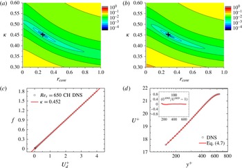
Figure 5(a) shows contours of errors $E_{r}$
for DNS channel data at
$E_{r}$
for DNS channel data at $Re_{\unicode[STIX]{x1D70F}}=650$
(Iwamoto et al.
Reference Iwamoto, Suzuki and Kasagi2002), for which we find
$Re_{\unicode[STIX]{x1D70F}}=650$
(Iwamoto et al.
Reference Iwamoto, Suzuki and Kasagi2002), for which we find $\unicode[STIX]{x1D705}^{Opt}\approx 0.452$
and
$\unicode[STIX]{x1D705}^{Opt}\approx 0.452$
and $r_{core}^{Opt}\approx 0.26$
. Also, at
$r_{core}^{Opt}\approx 0.26$
. Also, at $Re_{\unicode[STIX]{x1D70F}}=940$
(Hoyas & Jimenez Reference Hoyas and Jimenez2006),
$Re_{\unicode[STIX]{x1D70F}}=940$
(Hoyas & Jimenez Reference Hoyas and Jimenez2006), $\unicode[STIX]{x1D705}^{Opt}\approx 0.447$
and
$\unicode[STIX]{x1D705}^{Opt}\approx 0.447$
and $r_{core}^{Opt}\approx 0.31$
(figure 5
b). The results are consistent with previously reported values obtained through the compensated plot of the stress length function (in figure 3). The consistency of the method is further checked by verifying (4.7), i.e. using the scaling function
$r_{core}^{Opt}\approx 0.31$
(figure 5
b). The results are consistent with previously reported values obtained through the compensated plot of the stress length function (in figure 3). The consistency of the method is further checked by verifying (4.7), i.e. using the scaling function $f$
and the mean defect velocity,
$f$
and the mean defect velocity, $U_{d}^{+DNS}$
, to display a linear relation. Taking
$U_{d}^{+DNS}$
, to display a linear relation. Taking $Re_{\unicode[STIX]{x1D70F}}=650$
for example, figure 5(c) shows a clear linear relation with slope 0.452 for the entire outer region from
$Re_{\unicode[STIX]{x1D70F}}=650$
for example, figure 5(c) shows a clear linear relation with slope 0.452 for the entire outer region from $y^{+}=150$
to
$y^{+}=150$
to $y^{+}=Re_{\unicode[STIX]{x1D70F}}$
. Figure 5(d) shows that the theoretical MVP according to (4.7) (with three parameters
$y^{+}=Re_{\unicode[STIX]{x1D70F}}$
. Figure 5(d) shows that the theoretical MVP according to (4.7) (with three parameters $U_{c}^{+DNS}=21.54$
;
$U_{c}^{+DNS}=21.54$
; $r_{core}=0.26$
and
$r_{core}=0.26$
and $\unicode[STIX]{x1D705}=0.452$
) agrees very well with DNS data, with small errors, bounded within 0.1 % (see inset), indicating high-quality measurements. Therefore, on average, we choose
$\unicode[STIX]{x1D705}=0.452$
) agrees very well with DNS data, with small errors, bounded within 0.1 % (see inset), indicating high-quality measurements. Therefore, on average, we choose $\unicode[STIX]{x1D705}\approx 0.45$
and
$\unicode[STIX]{x1D705}\approx 0.45$
and $r_{core}\approx 0.27$
for current DNS data.
$r_{core}\approx 0.27$
for current DNS data.
A further consistency check is carried out by fixing $\unicode[STIX]{x1D705}=0.45,r_{core}=0.27$
and displaying the resulting outer MVPs using (4.6) for channels and pipes, as shown in figure 6, which are in excellent agreement with the data. This fully demonstrates the validity of the bulk-flow structure, i.e.
$\unicode[STIX]{x1D705}=0.45,r_{core}=0.27$
and displaying the resulting outer MVPs using (4.6) for channels and pipes, as shown in figure 6, which are in excellent agreement with the data. This fully demonstrates the validity of the bulk-flow structure, i.e. $1-r^{4}$
for channel and
$1-r^{4}$
for channel and $1-r^{5}$
for pipe. Note that (4.6) can be rewritten as
$1-r^{5}$
for pipe. Note that (4.6) can be rewritten as
 $$\begin{eqnarray}U_{c}^{+}-U^{+}=G(r);\quad G(r)=\int _{0}^{r}\frac{mr^{\prime }[(1+{r_{core}}^{2})/({r^{\prime }}^{2}+{r_{core}}^{2})]^{1/4}}{\unicode[STIX]{x1D705}(1-{r^{\prime }}^{m})}\,\text{d}r^{\prime }.\end{eqnarray}$$
We refer to $G$
as the wake function for channel and pipe flows.
$G$
as the wake function for channel and pipe flows.

It is interesting to compare our current results with the analysis by Klewicki (Reference Klewicki2013), who introduced a characteristic length scale $L_{width}^{+}=O(\unicode[STIX]{x1D6FD}^{-1/2})$
where
$L_{width}^{+}=O(\unicode[STIX]{x1D6FD}^{-1/2})$
where $\unicode[STIX]{x1D6FD}=\text{d}W^{+}/\text{d}y^{+}+\,1/Re_{\unicode[STIX]{x1D70F}}=-\text{d}S^{+}/\text{d}y^{+}$
(according to the mean-momentum equation). From our bulk solution
$\unicode[STIX]{x1D6FD}=\text{d}W^{+}/\text{d}y^{+}+\,1/Re_{\unicode[STIX]{x1D70F}}=-\text{d}S^{+}/\text{d}y^{+}$
(according to the mean-momentum equation). From our bulk solution $S^{+}=\sqrt{W^{+}}/\ell _{uv}^{+}\approx m\sqrt{r}/\unicode[STIX]{x1D705}(1-r^{m})Re_{\unicode[STIX]{x1D70F}}=m\sqrt{r}/\unicode[STIX]{x1D705}y^{+}(1+r+\cdots +r^{m-1})$
, it follows that, for the asymptotically large
$S^{+}=\sqrt{W^{+}}/\ell _{uv}^{+}\approx m\sqrt{r}/\unicode[STIX]{x1D705}(1-r^{m})Re_{\unicode[STIX]{x1D70F}}=m\sqrt{r}/\unicode[STIX]{x1D705}y^{+}(1+r+\cdots +r^{m-1})$
, it follows that, for the asymptotically large $Re$
’s,
$Re$
’s, $S^{+}\approx (\unicode[STIX]{x1D705}y^{+})^{-1}$
as
$S^{+}\approx (\unicode[STIX]{x1D705}y^{+})^{-1}$
as $r\rightarrow 1$
; then
$r\rightarrow 1$
; then $L_{width}^{+}\propto \sqrt{\unicode[STIX]{x1D705}}y^{+}$
, consistent with the results of Klewicki (Reference Klewicki2013).
$L_{width}^{+}\propto \sqrt{\unicode[STIX]{x1D705}}y^{+}$
, consistent with the results of Klewicki (Reference Klewicki2013).
Finally, descriptions of entire MVP (lines) for channel and pipe flows are given in figure 7 using (3.27) and $\unicode[STIX]{x1D70F}^{+}=1-y^{+}/Re_{\unicode[STIX]{x1D70F}}$
. The agreement is strong between predictions and data, as shown in the inset figures: the relative errors are bounded within 1 % at every measured point. Hence, through a multi-layer stress length function we obtain accurate descriptions of MVP for wall flows.
$\unicode[STIX]{x1D70F}^{+}=1-y^{+}/Re_{\unicode[STIX]{x1D70F}}$
. The agreement is strong between predictions and data, as shown in the inset figures: the relative errors are bounded within 1 % at every measured point. Hence, through a multi-layer stress length function we obtain accurate descriptions of MVP for wall flows.
Predictions of MVP through (3.27) (solid lines) compared with DNS data (symbols) of channel (a) and pipe (b) flows. The insets show the relative errors, i.e. $100\times (1-U^{DNS}/U^{SED})$
, uniformly bounded within 1 % (dashed lines) for the entire flow region. The data are the same as in figure 1.
$100\times (1-U^{DNS}/U^{SED})$
, uniformly bounded within 1 % (dashed lines) for the entire flow region. The data are the same as in figure 1.
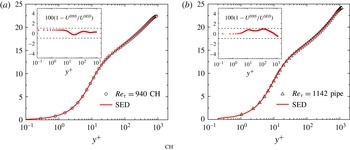
To examine the sensitivity of the ansatz in predicting the mean velocity $U(\,y)$
, we have computed
$U(\,y)$
, we have computed $U(\,y)$
for varying parameters (
$U(\,y)$
for varying parameters ( $\unicode[STIX]{x1D705},y_{sub}^{+},y_{buf}^{+},r_{core},p$
) in (3.27). It turns out that
$\unicode[STIX]{x1D705},y_{sub}^{+},y_{buf}^{+},r_{core},p$
) in (3.27). It turns out that $\unicode[STIX]{x1D705}$
is the most sensitive parameter, whose 2 % variation yields a 2 % change in the MVP. In contrast, for the same change of MVP,
$\unicode[STIX]{x1D705}$
is the most sensitive parameter, whose 2 % variation yields a 2 % change in the MVP. In contrast, for the same change of MVP, $y_{buf}^{+}$
needs to be changed by 4 %,
$y_{buf}^{+}$
needs to be changed by 4 %, $y_{sub}^{+}$
by 25 % and
$y_{sub}^{+}$
by 25 % and $r_{core}$
by 50 %. In addition, the transition sharpness
$r_{core}$
by 50 %. In addition, the transition sharpness $p$
is the least sensitive parameter: by varying current
$p$
is the least sensitive parameter: by varying current $p=4$
to either 2 or 6, changes the MVP by no more than 1 %. Thus, the most sensitive parameters are layer thickness and the Karman constant. Note that the scaling exponents are also important to quantify the MVP, but they are not fitting parameters, as they are either determined by boundary conditions or predicted theoretically.
$p=4$
to either 2 or 6, changes the MVP by no more than 1 %. Thus, the most sensitive parameters are layer thickness and the Karman constant. Note that the scaling exponents are also important to quantify the MVP, but they are not fitting parameters, as they are either determined by boundary conditions or predicted theoretically.
4.2 Validation by experimental data for high
$Re$

Given the fact that the multi-layer formula is verified and the parameters are determined by the DNS data, it is important to compare the predictions with experimental data at higher $Re$
to confirm whether the candidate solutions proposed here are generally valid for all Reynolds numbers. Below, we compare our theoretical prediction with experimental data: channel-flow data from Melbourne (Monty Reference Monty2005) (for
$Re$
to confirm whether the candidate solutions proposed here are generally valid for all Reynolds numbers. Below, we compare our theoretical prediction with experimental data: channel-flow data from Melbourne (Monty Reference Monty2005) (for $Re_{\unicode[STIX]{x1D70F}}$
varying from 1170 to 4042) and pipe-flow data from Princeton (Zagarola & Smits Reference Zagarola and Smits1998) (for
$Re_{\unicode[STIX]{x1D70F}}$
varying from 1170 to 4042) and pipe-flow data from Princeton (Zagarola & Smits Reference Zagarola and Smits1998) (for $Re_{\unicode[STIX]{x1D70F}}$
varying from 76 100 to 528 550), as shown in figure 8. The comparison shows that the present formalism yields a quantitative description with good accuracy over a wide range of
$Re_{\unicode[STIX]{x1D70F}}$
varying from 76 100 to 528 550), as shown in figure 8. The comparison shows that the present formalism yields a quantitative description with good accuracy over a wide range of $Re$
(i.e. errors are mostly bounded within 1 %), with a universal
$Re$
(i.e. errors are mostly bounded within 1 %), with a universal $\unicode[STIX]{x1D705}\approx 0.45$
but a slight change of
$\unicode[STIX]{x1D705}\approx 0.45$
but a slight change of $y_{buf}^{+}$
and
$y_{buf}^{+}$
and $r_{core}$
, both growing slowly as
$r_{core}$
, both growing slowly as $Re$
increases for
$Re$
increases for $Re_{\unicode[STIX]{x1D70F}}$
below 5000 but becoming constants (
$Re_{\unicode[STIX]{x1D70F}}$
below 5000 but becoming constants ( $y_{buf}^{+}\approx 44$
,
$y_{buf}^{+}\approx 44$
, $r_{core}\approx 0.5$
) for
$r_{core}\approx 0.5$
) for $Re_{\unicode[STIX]{x1D70F}}$
over 5000. Such a transition around
$Re_{\unicode[STIX]{x1D70F}}$
over 5000. Such a transition around $Re_{\unicode[STIX]{x1D70F}}=5000$
is also noted but not explained by Marusic et al. (Reference Marusic, McKeon, Monkewitz, Nagib, Smits and Sreenivasan2010).
$Re_{\unicode[STIX]{x1D70F}}=5000$
is also noted but not explained by Marusic et al. (Reference Marusic, McKeon, Monkewitz, Nagib, Smits and Sreenivasan2010).
MVPs for the entire flow (3.27) (solid lines) compared with experimental data (symbols) of channel (a) and pipe (c) flows. Experimental data for channel flow are from Melbourne (Monty Reference Monty2005) and from Princeton (Zagarola & Smits Reference Zagarola and Smits1998) for pipe flow. Each profile has been vertically shifted for a better display. (b,d) Show the relative errors of channel and pipe flows, respectively, mostly bounded within 1 % (dashed lines) for the entire flow region.
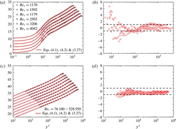
5 Discussions and concluding remarks
Several recent studies of the MVP are noteworthy. Monkewitz et al. (Reference Monkewitz, Chauhan and Nagib2007) and Nagib & Chauhan (Reference Nagib and Chauhan2008) (i.e. the MCN model) have made a tremendous effort to parameterize the entire MVP of channel, pipe and TBL, which concludes that the classical description (an inner–outer two-layer model with a logarithmic overlap region) is better than the competing power-law model. However, more than 10 fitting parameters defying any physical explanation are needed for each canonical flow, and the parameter variations among different flows are hardly intuitive. Moreover, the choice of wake functions has no sound physical basis and $\unicode[STIX]{x1D705}$
as a free-fitting parameter is called the ‘Karman coefficient’. Another model, by Nickels (Reference Nickels2004), employs a three-layer description (with an explicit logarithmic layer), but the switch from channel and pipe flows to the TBL has no justification. In addition, in Nickels’s model
$\unicode[STIX]{x1D705}$
as a free-fitting parameter is called the ‘Karman coefficient’. Another model, by Nickels (Reference Nickels2004), employs a three-layer description (with an explicit logarithmic layer), but the switch from channel and pipe flows to the TBL has no justification. In addition, in Nickels’s model $\unicode[STIX]{x1D705}$
is also a fitting parameter with no discussion of its universality and with no attempt to determine wake parameters to predict the full MVP. Del Alamo & Jimenez (Reference Del Alamo and Jimenez2006) also proposed a model for turbulent eddy viscosity, following Reynolds & Hussain (Reference Reynolds and Hussain1972), which leads to a closure description of the MVP in channel flows with no intent to generalize to the TBL is reported. A physical model by L’vov et al. (Reference L’vov, Procaccia and Rudenko2008) addresses explicitly effects of turbulent fluctuations on the mean velocity using three characteristic length scales, but then still employs an empirical wake function (by inspecting DNS data) for describing channel and pipe flows, without extending the analysis to the TBL. In summary, all existing quantitative models (Nickels Reference Nickels2004; Del Alamo & Jimenez Reference Del Alamo and Jimenez2006; Monkewitz et al.
Reference Monkewitz, Chauhan and Nagib2007; Panton Reference Panton2007; L’vov et al.
Reference L’vov, Procaccia and Rudenko2008) for wall turbulence remain essentially empirical.
$\unicode[STIX]{x1D705}$
is also a fitting parameter with no discussion of its universality and with no attempt to determine wake parameters to predict the full MVP. Del Alamo & Jimenez (Reference Del Alamo and Jimenez2006) also proposed a model for turbulent eddy viscosity, following Reynolds & Hussain (Reference Reynolds and Hussain1972), which leads to a closure description of the MVP in channel flows with no intent to generalize to the TBL is reported. A physical model by L’vov et al. (Reference L’vov, Procaccia and Rudenko2008) addresses explicitly effects of turbulent fluctuations on the mean velocity using three characteristic length scales, but then still employs an empirical wake function (by inspecting DNS data) for describing channel and pipe flows, without extending the analysis to the TBL. In summary, all existing quantitative models (Nickels Reference Nickels2004; Del Alamo & Jimenez Reference Del Alamo and Jimenez2006; Monkewitz et al.
Reference Monkewitz, Chauhan and Nagib2007; Panton Reference Panton2007; L’vov et al.
Reference L’vov, Procaccia and Rudenko2008) for wall turbulence remain essentially empirical.
In this paper, we present a derivation of the multi-layer formula for the stress length function, motivated from an innovative Lie-group symmetry analysis. The Lie-group formalism expresses the mean-momentum equation in terms of the group invariants, which is not closed and hence cannot be solved directly. Then, a specific set of ansatz are postulated for group invariants associated with the stress length and its derivative, then the multi-layer analytical structure is predicted, which yields expressions for the mean shear, the Reynolds stress and hence the mean velocity over the entire domain. While the multi-layer structure follows from the symmetry assumption, which is rigorously justified locally for the viscous sublayer and the central core layer, the parameters quantifying the multi-layer are obtained by a mixture of phenomenological reasoning and empirical fitting to data. The final results are reasonable, since the current description provides a simple distinction between channel, pipe and TBL ( $m=4$
for a flat wall while
$m=4$
for a flat wall while $m=5$
for a cylindrical wall; the presence of the central core layer for internal flows while absent for the external flow). It is particularly interesting to mention that
$m=5$
for a cylindrical wall; the presence of the central core layer for internal flows while absent for the external flow). It is particularly interesting to mention that $\unicode[STIX]{x1D705}$
and
$\unicode[STIX]{x1D705}$
and $y_{sub}^{+}$
are checked to be universal constants for three canonical wall flows, while
$y_{sub}^{+}$
are checked to be universal constants for three canonical wall flows, while $y_{buf}^{+}$
possesses modest
$y_{buf}^{+}$
possesses modest $Re$
-dependence (which will be reported in the near future). Hence, a unified description of three canonical wall-bounded flows is achieved.
$Re$
-dependence (which will be reported in the near future). Hence, a unified description of three canonical wall-bounded flows is achieved.
As explained in previous sections, the multi-layered structure identified here is closely associated with the different balances between the terms in the turbulent kinetic-energy equation (i.e. $SW+\unicode[STIX]{x1D6F1}_{p}=\unicode[STIX]{x1D700}$
, where
$SW+\unicode[STIX]{x1D6F1}_{p}=\unicode[STIX]{x1D700}$
, where $SW$
is the production,
$SW$
is the production, $\unicode[STIX]{x1D700}$
is the dissipation and
$\unicode[STIX]{x1D700}$
is the dissipation and $\unicode[STIX]{x1D6F1}_{p}$
is the spatial transport effect). This is illustrated again by the ratio of
$\unicode[STIX]{x1D6F1}_{p}$
is the spatial transport effect). This is illustrated again by the ratio of $SW$
to
$SW$
to $\unicode[STIX]{x1D700}$
shown in figure 9. One can see that the viscous sublayer is characterized by
$\unicode[STIX]{x1D700}$
shown in figure 9. One can see that the viscous sublayer is characterized by $SW\ll \unicode[STIX]{x1D700}\approx \unicode[STIX]{x1D6F1}_{p}$
; the buffer layer by the same order of
$SW\ll \unicode[STIX]{x1D700}\approx \unicode[STIX]{x1D6F1}_{p}$
; the buffer layer by the same order of $SW$
,
$SW$
, $\unicode[STIX]{x1D700}$
and
$\unicode[STIX]{x1D700}$
and $|\unicode[STIX]{x1D6F1}_{p}|$
; the bulk region by
$|\unicode[STIX]{x1D6F1}_{p}|$
; the bulk region by $SW\approx \unicode[STIX]{x1D700}\gg |\unicode[STIX]{x1D6F1}_{p}|$
; and the core layer by
$SW\approx \unicode[STIX]{x1D700}\gg |\unicode[STIX]{x1D6F1}_{p}|$
; and the core layer by $SW\ll \unicode[STIX]{x1D700}\approx \unicode[STIX]{x1D6F1}_{p}$
. Thus, different balances of the kinetic-energy equation terms give rise to different layers of the stress length function.
$SW\ll \unicode[STIX]{x1D700}\approx \unicode[STIX]{x1D6F1}_{p}$
. Thus, different balances of the kinetic-energy equation terms give rise to different layers of the stress length function.
Ratio of production to dissipation terms of the kinetic-energy equation in a DNS channel at $Re_{\unicode[STIX]{x1D70F}}=650$
(Iwamoto et al.
Reference Iwamoto, Suzuki and Kasagi2002). The boundaries of viscous sublayer, buffer layer, bulk region and core layer are located at
$Re_{\unicode[STIX]{x1D70F}}=650$
(Iwamoto et al.
Reference Iwamoto, Suzuki and Kasagi2002). The boundaries of viscous sublayer, buffer layer, bulk region and core layer are located at $y_{sub}^{+}\approx 9.7$
,
$y_{sub}^{+}\approx 9.7$
, $y_{buf}^{+}\approx 41$
and
$y_{buf}^{+}\approx 41$
and $r_{core}\approx 0.27$
, respectively.
$r_{core}\approx 0.27$
, respectively.
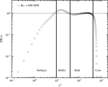
Note that the universality of $\unicode[STIX]{x1D705}$
is an important issue. In the literature, the
$\unicode[STIX]{x1D705}$
is an important issue. In the literature, the $\unicode[STIX]{x1D705}$
values are under vivid debates varying over a fairly wide range (Marusic et al.
Reference Marusic, McKeon, Monkewitz, Nagib, Smits and Sreenivasan2010). One of the major uncertainties in measuring
$\unicode[STIX]{x1D705}$
values are under vivid debates varying over a fairly wide range (Marusic et al.
Reference Marusic, McKeon, Monkewitz, Nagib, Smits and Sreenivasan2010). One of the major uncertainties in measuring $\unicode[STIX]{x1D705}$
is due to the arbitrary setting of the overlap region, which obviously leads to different values of
$\unicode[STIX]{x1D705}$
is due to the arbitrary setting of the overlap region, which obviously leads to different values of $\unicode[STIX]{x1D705}$
(Alfredsson et al.
Reference Alfredsson, Imayamaa, Lingwood, Orlu and Segalini2013; Segalini et al.
Reference Segalini, Orlu and Alfredsson2013). Taking the Princeton pipe data, for example, while Zagarola & Smits (Reference Zagarola and Smits1998) chose an overlap region of
$\unicode[STIX]{x1D705}$
(Alfredsson et al.
Reference Alfredsson, Imayamaa, Lingwood, Orlu and Segalini2013; Segalini et al.
Reference Segalini, Orlu and Alfredsson2013). Taking the Princeton pipe data, for example, while Zagarola & Smits (Reference Zagarola and Smits1998) chose an overlap region of $600<y^{+}<0.07Re_{\unicode[STIX]{x1D70F}}$
, yielding
$600<y^{+}<0.07Re_{\unicode[STIX]{x1D70F}}$
, yielding $\unicode[STIX]{x1D705}=0.436$
, McKeon et al. (Reference McKeon, Li, Jiang, Morrison and Smits2004) chose the region of
$\unicode[STIX]{x1D705}=0.436$
, McKeon et al. (Reference McKeon, Li, Jiang, Morrison and Smits2004) chose the region of $600<y^{+}<0.12Re_{\unicode[STIX]{x1D70F}}$
, yielding
$600<y^{+}<0.12Re_{\unicode[STIX]{x1D70F}}$
, yielding $\unicode[STIX]{x1D705}=0.421$
. Recently, Marusic et al. (Reference Marusic, Monty, Hultmark and Smits2013) defined a logarithmic region (in
$\unicode[STIX]{x1D705}=0.421$
. Recently, Marusic et al. (Reference Marusic, Monty, Hultmark and Smits2013) defined a logarithmic region (in $y^{+}$
) from
$y^{+}$
) from $3\sqrt{Re_{\unicode[STIX]{x1D70F}}}$
to
$3\sqrt{Re_{\unicode[STIX]{x1D70F}}}$
to $0.15Re_{\unicode[STIX]{x1D70F}}$
and suggested
$0.15Re_{\unicode[STIX]{x1D70F}}$
and suggested $\unicode[STIX]{x1D705}$
to be 0.39 for Princeton pipe data. Another recent effort by Nagib & Chauhan (Reference Nagib and Chauhan2008) involves determining
$\unicode[STIX]{x1D705}$
to be 0.39 for Princeton pipe data. Another recent effort by Nagib & Chauhan (Reference Nagib and Chauhan2008) involves determining $\unicode[STIX]{x1D705}$
freely in (artificially) composed asymptotic expansions. In contrast, here we have derived a geometry-dependent bulk-flow structure (i.e.
$\unicode[STIX]{x1D705}$
freely in (artificially) composed asymptotic expansions. In contrast, here we have derived a geometry-dependent bulk-flow structure (i.e. $1-r^{m}$
with
$1-r^{m}$
with $m=4$
for channel and TBL and 5 for pipe), thus removing the need for defining the overlap region. Our theory then defines
$m=4$
for channel and TBL and 5 for pipe), thus removing the need for defining the overlap region. Our theory then defines $\unicode[STIX]{x1D705}$
as a global coefficient valid for the entire outer flow (including the overlap region), which coincides with Prandtl’s original definition close to the wall for asymptotically large
$\unicode[STIX]{x1D705}$
as a global coefficient valid for the entire outer flow (including the overlap region), which coincides with Prandtl’s original definition close to the wall for asymptotically large $Re^{\prime }$
s. The value 0.45 is measured here from DNS data in figure 5, and is verified to a great extent to higher
$Re^{\prime }$
s. The value 0.45 is measured here from DNS data in figure 5, and is verified to a great extent to higher $Re$
by a number of experimental MVPs for channel, pipe and TBL (She et al.
Reference She, Wu, Chen and Hussain2012; Chen et al.
Reference Chen, Hussain and She2016b
; Chen & She Reference Chen and She2016). An additional support of this new Karman constant stems from a recent study of the Wilcox
$Re$
by a number of experimental MVPs for channel, pipe and TBL (She et al.
Reference She, Wu, Chen and Hussain2012; Chen et al.
Reference Chen, Hussain and She2016b
; Chen & She Reference Chen and She2016). An additional support of this new Karman constant stems from a recent study of the Wilcox $k{-}\unicode[STIX]{x1D714}$
model (Chen et al.
Reference Chen, Hussain and She2016a
): by changing
$k{-}\unicode[STIX]{x1D714}$
model (Chen et al.
Reference Chen, Hussain and She2016a
): by changing $\unicode[STIX]{x1D705}=0.41$
in the original
$\unicode[STIX]{x1D705}=0.41$
in the original $k{-}\unicode[STIX]{x1D714}$
model (Wilcox Reference Wilcox2006) to 0.45, one immediately obtains much better agreement with Princeton’s experimental MVPs near the wall, with significant improvement at high
$k{-}\unicode[STIX]{x1D714}$
model (Wilcox Reference Wilcox2006) to 0.45, one immediately obtains much better agreement with Princeton’s experimental MVPs near the wall, with significant improvement at high $Re$
’s. Thus, our results support a universal
$Re$
’s. Thus, our results support a universal $\unicode[STIX]{x1D705}$
for three canonical wall flows, which should be verified against more data.
$\unicode[STIX]{x1D705}$
for three canonical wall flows, which should be verified against more data.
It is natural to ask whether the stress length is the only choice as a symmetry-preserved variable. Actually, the prediction will be different if a different quantity, e.g. the eddy viscosity $\unicode[STIX]{x1D708}_{T}^{+}=W^{+}/S^{+}$
, is assumed to follow the invariant ansatz. Note that if one carries the transformation (2.9) on
$\unicode[STIX]{x1D708}_{T}^{+}=W^{+}/S^{+}$
, is assumed to follow the invariant ansatz. Note that if one carries the transformation (2.9) on $\unicode[STIX]{x1D708}_{T}^{+}$
in the balance equation (2.6), the transformed eddy viscosity then reads
$\unicode[STIX]{x1D708}_{T}^{+}$
in the balance equation (2.6), the transformed eddy viscosity then reads $\unicode[STIX]{x1D708}_{T}^{+\ast }=\ell _{uv}^{+\ast 2}S^{+\ast }=\ell _{uv}^{+2}S^{+}=\unicode[STIX]{x1D708}_{T}^{+}$
. In other words,
$\unicode[STIX]{x1D708}_{T}^{+\ast }=\ell _{uv}^{+\ast 2}S^{+\ast }=\ell _{uv}^{+2}S^{+}=\unicode[STIX]{x1D708}_{T}^{+}$
. In other words, $\unicode[STIX]{x1D708}_{T}^{+}$
is itself a dilatation invariant. However, unlike
$\unicode[STIX]{x1D708}_{T}^{+}$
is itself a dilatation invariant. However, unlike $I_{1}$
or
$I_{1}$
or $I_{2}$
for the stress length, neither the scalar nor the differential invariant of
$I_{2}$
for the stress length, neither the scalar nor the differential invariant of $\unicode[STIX]{x1D708}_{T}^{+}$
is a true constant in any of the layers, since neither
$\unicode[STIX]{x1D708}_{T}^{+}$
is a true constant in any of the layers, since neither $\unicode[STIX]{x1D708}_{T}^{+}=\text{const.}$
nor
$\unicode[STIX]{x1D708}_{T}^{+}=\text{const.}$
nor $\unicode[STIX]{x1D708}_{T}^{+}\propto \ln (y^{+})$
is supported by empirical data. In practice, choosing
$\unicode[STIX]{x1D708}_{T}^{+}\propto \ln (y^{+})$
is supported by empirical data. In practice, choosing $\ell _{uv}$
to follow the dilatation invariant ansatz yields simple and valid analytical forms for all relevant functions (e.g.
$\ell _{uv}$
to follow the dilatation invariant ansatz yields simple and valid analytical forms for all relevant functions (e.g. $S^{+}$
,
$S^{+}$
, $W^{+}$
).
$W^{+}$
).
Also, what does the symmetry analysis using the Lie-group formalism add to our understanding beyond making a direct postulate of power law? The answer is that a Lie-group formalism guarantees that the RANS equation remains invariant under the (dilatation) group of transformation and any invariant solution ansatz used here also guarantees that a transformed solution satisfies the RANS equation. While the power-law form of the stress length can be motivated from simple scaling arguments, the ansatz of the second and third kinds, a defect-power-law form for the bulk flow and a series of scaling matched forms, would be difficult to guess. This last ansatz is invoked by the simple continuity assumption about the variation of the local group invariants. A future task is to combine the stress length function with the study of coherent structures. For example, by assuming that the stress length indeed describes the integral scale eddies, one may extend the Townsend–Perry wall-attached eddy theory (Townsend Reference Townsend1976; Perry & Chong Reference Perry and Chong1982; Perry, Henbest & Chong Reference Perry, Henbest and Chong1986).
The present approach also can be applied to describe the distribution of streamwise fluctuation intensity (Chen et al.
Reference Chen, Wei, Hussain and She2015). In analogy to the stress length function $\ell _{uv}$
defined in (1.4), it is natural to define
$\ell _{uv}$
defined in (1.4), it is natural to define $\ell _{uu}=\langle u^{\prime }u^{\prime }\rangle ^{1/2}/\unicode[STIX]{x2202}_{y}U$
, which leads to
$\ell _{uu}=\langle u^{\prime }u^{\prime }\rangle ^{1/2}/\unicode[STIX]{x2202}_{y}U$
, which leads to $\langle u^{\prime }u^{\prime }\rangle =-\langle u^{\prime }v^{\prime }\rangle (\ell _{uu}/\ell _{uv})^{2}$
. Similar to
$\langle u^{\prime }u^{\prime }\rangle =-\langle u^{\prime }v^{\prime }\rangle (\ell _{uu}/\ell _{uv})^{2}$
. Similar to $\ell _{uv}^{\wedge Outer}$
in (3.24), a composite formula for
$\ell _{uv}^{\wedge Outer}$
in (3.24), a composite formula for $\ell _{uu}^{\wedge }$
connecting the bulk and the core layer of pipe flows is suggested as
$\ell _{uu}^{\wedge }$
connecting the bulk and the core layer of pipe flows is suggested as
 $$\begin{eqnarray}\ell _{uu}^{\wedge }=\unicode[STIX]{x1D705}^{\prime }(1-r)^{\unicode[STIX]{x0394}\unicode[STIX]{x1D6FE}}(1-r^{5})[1+(r_{core}/r)^{2}]^{1/2}/(5Z_{c}^{\prime }),\end{eqnarray}$$
where $Z_{c}^{\prime }=(1+r_{core}^{2})^{1/2}$
. Here,
$Z_{c}^{\prime }=(1+r_{core}^{2})^{1/2}$
. Here, $\ell _{uu}^{\wedge }$
differs from
$\ell _{uu}^{\wedge }$
differs from $\ell _{uv}^{\wedge }$
by the presence of an abnormal scaling
$\ell _{uv}^{\wedge }$
by the presence of an abnormal scaling $\unicode[STIX]{x0394}\unicode[STIX]{x1D6FE}\neq 0$
quantifying a meso-layer and a different core layer scaling at the centreline (
$\unicode[STIX]{x0394}\unicode[STIX]{x1D6FE}\neq 0$
quantifying a meso-layer and a different core layer scaling at the centreline ( $\ell _{uu}^{\wedge }\propto 1/r$
for
$\ell _{uu}^{\wedge }\propto 1/r$
for $r\rightarrow 0$
due to a finite
$r\rightarrow 0$
due to a finite $\langle u^{\prime }u^{\prime }\rangle$
at the centreline). Note that
$\langle u^{\prime }u^{\prime }\rangle$
at the centreline). Note that $\unicode[STIX]{x0394}\unicode[STIX]{x1D6FE}=0$
yields
$\unicode[STIX]{x0394}\unicode[STIX]{x1D6FE}=0$
yields $|\langle u^{\prime }u^{\prime }\rangle /\langle u^{\prime }v^{\prime }\rangle |^{1/2}=\ell _{uu}/\ell _{uv}\approx \unicode[STIX]{x1D705}^{\prime }/\unicode[STIX]{x1D705}$
in the overlap region, which indicates
$|\langle u^{\prime }u^{\prime }\rangle /\langle u^{\prime }v^{\prime }\rangle |^{1/2}=\ell _{uu}/\ell _{uv}\approx \unicode[STIX]{x1D705}^{\prime }/\unicode[STIX]{x1D705}$
in the overlap region, which indicates $\langle u^{\prime }u^{\prime }\rangle \approx (\unicode[STIX]{x1D705}^{\prime }/\unicode[STIX]{x1D705})^{2}u_{\unicode[STIX]{x1D70F}}^{2}$
, a constant streamwise kinetic energy. However, this contrasts with a recent observation of an outer peak of
$\langle u^{\prime }u^{\prime }\rangle \approx (\unicode[STIX]{x1D705}^{\prime }/\unicode[STIX]{x1D705})^{2}u_{\unicode[STIX]{x1D70F}}^{2}$
, a constant streamwise kinetic energy. However, this contrasts with a recent observation of an outer peak of $\langle u^{\prime }u^{\prime }\rangle$
in high
$\langle u^{\prime }u^{\prime }\rangle$
in high $Re$
pipe (Hultmark et al.
Reference Hultmark, Vallikivi, Bailey and Smits2012). In other words, the presence of the outer peak implies that
$Re$
pipe (Hultmark et al.
Reference Hultmark, Vallikivi, Bailey and Smits2012). In other words, the presence of the outer peak implies that $\unicode[STIX]{x0394}\unicode[STIX]{x1D6FE}\neq 0$
.
$\unicode[STIX]{x0394}\unicode[STIX]{x1D6FE}\neq 0$
.
Thus, using (3.24) and (5.1), the outer streamwise kinetic-energy profile is given as
 $$\begin{eqnarray}\langle u^{\prime }u^{\prime }\rangle ^{+}=-\langle u^{\prime }v^{\prime }\rangle ^{+}(\ell _{uu}/\ell _{uv})^{2}\approx r(\unicode[STIX]{x1D705}^{\prime }/\unicode[STIX]{x1D705})^{2}(1-r)^{2\unicode[STIX]{x0394}\unicode[STIX]{x1D6FE}}(Z_{c}/Z_{c}^{\prime })^{2}[1+(r_{core}/r)^{2}]^{1/2}.\end{eqnarray}$$
With the values of $r_{core}=0.27$
,
$r_{core}=0.27$
, $\unicode[STIX]{x1D705}^{\prime }=0.80$
and
$\unicode[STIX]{x1D705}^{\prime }=0.80$
and $\unicode[STIX]{x0394}\unicode[STIX]{x1D6FE}=-0.06$
for
$\unicode[STIX]{x0394}\unicode[STIX]{x1D6FE}=-0.06$
for $\ell _{uu}$
, figure 10 shows good agreement between (5.2) and the data. Hence, the multi-layer ansatz and the length order functions give rise to a unified description of the mean velocity and kinetic-energy profiles. A complete description of the entire
$\ell _{uu}$
, figure 10 shows good agreement between (5.2) and the data. Hence, the multi-layer ansatz and the length order functions give rise to a unified description of the mean velocity and kinetic-energy profiles. A complete description of the entire $\langle u^{\prime }u^{\prime }\rangle$
,
$\langle u^{\prime }u^{\prime }\rangle$
, $\langle v^{\prime }v^{\prime }\rangle$
and
$\langle v^{\prime }v^{\prime }\rangle$
and $\langle w^{\prime }w^{\prime }\rangle$
profiles through
$\langle w^{\prime }w^{\prime }\rangle$
profiles through $\ell _{uu}$
,
$\ell _{uu}$
, $\ell _{vv}$
and
$\ell _{vv}$
and $\ell _{ww}$
can all be obtained similarly.
$\ell _{ww}$
can all be obtained similarly.


Finally, it is necessary to clarify the analytical part of current results from those obtained from data, where concerns may arise regarding the ‘derivation’ (or ‘prediction’) of the multi-layer structure. Here, let us summarize our three steps to define the invariant solution of the RANS equation and hence obtain the multi-layer structure. First, the theory chooses the length (order) function since length scale is essential to the description of turbulence. Second, the Lie-group argument is invoked to determine the analytical form of the stress length function, with the dilatation invariance from $y=0$
(the wall) and
$y=0$
(the wall) and $r=0$
(the centre of channel/pipe and the edge of the TBL). The composite formula over the entire flow region is obtained by matching the local dilatation invariants, and the wall and wake functions for the mean velocity are directly obtained from the mean-momentum equation. Finally, a variety of techniques are used to determine the values of the scaling exponents and layer thicknesses in the multi-layer formula, where phenomenological arguments and data fitting are involved only in this step. Thus the three steps constitute a general and systematic procedure. We have applied the approach to a variety of wall-bounded flows (channel, pipe, TBL, Rayleigh–Benard convection and Taylor–Coutte flow, etc.), and under the effects of compressibility (Zhang et al.
Reference Zhang, Bi, Hussain, Li and She2012; Wu et al.
Reference Wu, Bi, Hussain and She2017), roughness (She et al.
Reference She, Wu, Chen and Hussain2012) and pressure gradient, and these results will be communicated in the near future.
$r=0$
(the centre of channel/pipe and the edge of the TBL). The composite formula over the entire flow region is obtained by matching the local dilatation invariants, and the wall and wake functions for the mean velocity are directly obtained from the mean-momentum equation. Finally, a variety of techniques are used to determine the values of the scaling exponents and layer thicknesses in the multi-layer formula, where phenomenological arguments and data fitting are involved only in this step. Thus the three steps constitute a general and systematic procedure. We have applied the approach to a variety of wall-bounded flows (channel, pipe, TBL, Rayleigh–Benard convection and Taylor–Coutte flow, etc.), and under the effects of compressibility (Zhang et al.
Reference Zhang, Bi, Hussain, Li and She2012; Wu et al.
Reference Wu, Bi, Hussain and She2017), roughness (She et al.
Reference She, Wu, Chen and Hussain2012) and pressure gradient, and these results will be communicated in the near future.
Acknowledgements
We thank B. Cantwell and M. Oberlack for helpful discussions. Y. Wu contributed during the initial stages of this work. This work is supported by National Nature Science Fund 11221062, 11452002 and by MOST 973 project 2009CB724100.
Appendix A. Dilation group analysis for channel flow
The analysis consists of the following three standard steps. Step one is to define the symmetry transformations. For (2.6), a Lie-group transformation $S_{\unicode[STIX]{x1D700}}$
can be expressed as
$S_{\unicode[STIX]{x1D700}}$
can be expressed as
 $$\begin{eqnarray}\boldsymbol{t}^{\ast }=\unicode[STIX]{x1D6F7}(\boldsymbol{t},\boldsymbol{x},\unicode[STIX]{x1D700});\quad \boldsymbol{x}^{\ast }=\unicode[STIX]{x1D6F9}(\boldsymbol{t},\boldsymbol{x},\unicode[STIX]{x1D700}),\end{eqnarray}$$
where the superscript $\ast$
denotes transformed variables;
$\ast$
denotes transformed variables; $\boldsymbol{t}=(\,y^{+},Re_{\unicode[STIX]{x1D70F}})$
and
$\boldsymbol{t}=(\,y^{+},Re_{\unicode[STIX]{x1D70F}})$
and $\boldsymbol{x}=(U^{+},\ell _{uv}^{+})$
are independent and dependent variables, respectively; and
$\boldsymbol{x}=(U^{+},\ell _{uv}^{+})$
are independent and dependent variables, respectively; and $\unicode[STIX]{x1D6F7},\unicode[STIX]{x1D6F9}$
are analytical functions of
$\unicode[STIX]{x1D6F7},\unicode[STIX]{x1D6F9}$
are analytical functions of $\boldsymbol{t}$
,
$\boldsymbol{t}$
, $\boldsymbol{x}$
and a continuous parameter
$\boldsymbol{x}$
and a continuous parameter $\unicode[STIX]{x1D700}$
(note that a key step is to specify the independent
$\unicode[STIX]{x1D700}$
(note that a key step is to specify the independent $(\,y^{+},Re_{\unicode[STIX]{x1D70F}})$
and dependent variables (
$(\,y^{+},Re_{\unicode[STIX]{x1D70F}})$
and dependent variables ( $U^{+},\ell _{uv}^{+}$
). The next step is to follow the standard software to calculate the infinitesimals). Then the symmetry transformation satisfies
$U^{+},\ell _{uv}^{+}$
). The next step is to follow the standard software to calculate the infinitesimals). Then the symmetry transformation satisfies
 $$\begin{eqnarray}\mathbb{C}(\boldsymbol{t},\boldsymbol{x})=0\quad \Leftrightarrow \quad \mathbb{C}(\boldsymbol{t}^{\ast },\boldsymbol{x}^{\ast })=0.\end{eqnarray}$$
Note that $S_{\unicode[STIX]{x1D700}}$
can also be expressed in an infinitesimal form
$S_{\unicode[STIX]{x1D700}}$
can also be expressed in an infinitesimal form
 $$\begin{eqnarray}\displaystyle \boldsymbol{t}^{\ast }=\boldsymbol{t}+\overrightarrow{\unicode[STIX]{x1D709}}(\boldsymbol{t},\boldsymbol{x})\unicode[STIX]{x1D700}+O(\unicode[STIX]{x1D700}^{2});\quad \boldsymbol{x}^{\ast }=\boldsymbol{x}+\overrightarrow{\unicode[STIX]{x1D702}}(\boldsymbol{t},\boldsymbol{x})\unicode[STIX]{x1D700}+O(\unicode[STIX]{x1D700}^{2}), & & \displaystyle\end{eqnarray}$$
where $\overrightarrow{\unicode[STIX]{x1D709}}=\unicode[STIX]{x2202}\unicode[STIX]{x1D6F7}/\unicode[STIX]{x2202}\unicode[STIX]{x1D700}|_{\unicode[STIX]{x1D700}=0}=(\unicode[STIX]{x1D709}_{y^{+}},\unicode[STIX]{x1D709}_{Re_{\unicode[STIX]{x1D70F}}})$
and
$\overrightarrow{\unicode[STIX]{x1D709}}=\unicode[STIX]{x2202}\unicode[STIX]{x1D6F7}/\unicode[STIX]{x2202}\unicode[STIX]{x1D700}|_{\unicode[STIX]{x1D700}=0}=(\unicode[STIX]{x1D709}_{y^{+}},\unicode[STIX]{x1D709}_{Re_{\unicode[STIX]{x1D70F}}})$
and $\overrightarrow{\unicode[STIX]{x1D702}}=\unicode[STIX]{x2202}\unicode[STIX]{x1D6F9}/\unicode[STIX]{x2202}\unicode[STIX]{x1D700}|_{\unicode[STIX]{x1D700}=0}=(\unicode[STIX]{x1D702}_{U^{+}},\unicode[STIX]{x1D702}_{\ell _{uv}^{+}})$
are the so-called infinitesimals. Then Taylor expansion,
$\overrightarrow{\unicode[STIX]{x1D702}}=\unicode[STIX]{x2202}\unicode[STIX]{x1D6F9}/\unicode[STIX]{x2202}\unicode[STIX]{x1D700}|_{\unicode[STIX]{x1D700}=0}=(\unicode[STIX]{x1D702}_{U^{+}},\unicode[STIX]{x1D702}_{\ell _{uv}^{+}})$
are the so-called infinitesimals. Then Taylor expansion, $\mathbb{C}(\boldsymbol{t}^{\ast },\boldsymbol{x}^{\ast })=\mathbb{C}(\boldsymbol{t},\boldsymbol{x})+\unicode[STIX]{x1D700}X\mathbb{C}+O(\unicode[STIX]{x1D700}^{2})$
, yields the following equation for the infinitesimals:
$\mathbb{C}(\boldsymbol{t}^{\ast },\boldsymbol{x}^{\ast })=\mathbb{C}(\boldsymbol{t},\boldsymbol{x})+\unicode[STIX]{x1D700}X\mathbb{C}+O(\unicode[STIX]{x1D700}^{2})$
, yields the following equation for the infinitesimals:
 $$\begin{eqnarray}X\mathbb{C}|_{C=0}=\unicode[STIX]{x1D709}_{y^{+}}\frac{\unicode[STIX]{x2202}\mathbb{C}}{\unicode[STIX]{x2202}y^{+}}+\unicode[STIX]{x1D709}_{Re_{\unicode[STIX]{x1D70F}}}\frac{\unicode[STIX]{x2202}\mathbb{C}}{\unicode[STIX]{x2202}Re_{\unicode[STIX]{x1D70F}}}+\unicode[STIX]{x1D702}_{U^{+}}\frac{\unicode[STIX]{x2202}\mathbb{C}}{\unicode[STIX]{x2202}U^{+}}+\unicode[STIX]{x1D702}_{\ell _{uv}^{+}}\frac{\unicode[STIX]{x2202}\mathbb{C}}{\unicode[STIX]{x2202}\ell _{uv}^{+}}+X_{p}=0,\end{eqnarray}$$
where $X$
is the so called Lie-group operator and
$X$
is the so called Lie-group operator and $X_{p}$
, solved from
$X_{p}$
, solved from $\overrightarrow{\unicode[STIX]{x1D709}}$
and
$\overrightarrow{\unicode[STIX]{x1D709}}$
and $\overrightarrow{\unicode[STIX]{x1D702}}$
, is referred to as the ‘prolongation’ (of the group) by the contact condition (see Cantwell Reference Cantwell2002). The infinitesimals can be solved conveniently by software Maple13, yielding
$\overrightarrow{\unicode[STIX]{x1D702}}$
, is referred to as the ‘prolongation’ (of the group) by the contact condition (see Cantwell Reference Cantwell2002). The infinitesimals can be solved conveniently by software Maple13, yielding
 $$\begin{eqnarray}\displaystyle \unicode[STIX]{x1D709}_{y^{+}}=a_{1}y^{+}+b_{1},\quad \unicode[STIX]{x1D709}_{Re_{\unicode[STIX]{x1D70F}}}=a_{2}Re_{\unicode[STIX]{x1D70F}}, & & \displaystyle\end{eqnarray}$$
 $$\begin{eqnarray}\displaystyle \unicode[STIX]{x1D702}_{U^{+}}=(2a_{1}-a_{2})U^{+}+b_{2},\quad \unicode[STIX]{x1D702}_{\ell _{uv}^{+}}=(-a_{1}+a_{2})\ell _{uv}^{+}/2, & & \displaystyle\end{eqnarray}$$
where coefficients $a_{i}$
and
$a_{i}$
and $b_{i}$
(
$b_{i}$
( $i=1,2$
) are functions of
$i=1,2$
) are functions of $Re_{\unicode[STIX]{x1D70F}}$
denoting dilatations and translations, respectively. Now, the wall condition, i.e.
$Re_{\unicode[STIX]{x1D70F}}$
denoting dilatations and translations, respectively. Now, the wall condition, i.e. $U^{+^{\ast }}=\ell _{uv}^{+^{\ast }}=0$
at
$U^{+^{\ast }}=\ell _{uv}^{+^{\ast }}=0$
at $y^{+^{\ast }}=0$
, leads to
$y^{+^{\ast }}=0$
, leads to $b_{1}=b_{2}=0$
; thus, near the wall, only the dilatations (as opposed to translations) are permitted. Normalized with the parameter
$b_{1}=b_{2}=0$
; thus, near the wall, only the dilatations (as opposed to translations) are permitted. Normalized with the parameter $a_{1}$
, we have
$a_{1}$
, we have
 $$\begin{eqnarray}\displaystyle \unicode[STIX]{x1D709}_{y^{+}}=y^{+},\quad \unicode[STIX]{x1D709}_{Re_{\unicode[STIX]{x1D70F}}}=(1+2\unicode[STIX]{x1D6FC})Re_{\unicode[STIX]{x1D70F}}, & & \displaystyle\end{eqnarray}$$
 $$\begin{eqnarray}\displaystyle \unicode[STIX]{x1D702}_{U^{+}}=(1-2\unicode[STIX]{x1D6FC})U^{+},\quad \unicode[STIX]{x1D702}_{\ell _{uv}^{+}}=\unicode[STIX]{x1D6FC}\ell _{uv}^{+}, & & \displaystyle\end{eqnarray}$$
where $\unicode[STIX]{x1D6FC}=(-1+a_{2}/a_{1})/2$
is the only remaining parameter quantifying the local scaling of the stress length.
$\unicode[STIX]{x1D6FC}=(-1+a_{2}/a_{1})/2$
is the only remaining parameter quantifying the local scaling of the stress length.
Step two is to define group invariants, which are obtained by solving the characteristic equations $\text{d}t_{i}/\text{d}\unicode[STIX]{x1D709}_{i}=\text{d}x_{i}/\text{d}\unicode[STIX]{x1D702}_{i}$
, for our case, written as
$\text{d}t_{i}/\text{d}\unicode[STIX]{x1D709}_{i}=\text{d}x_{i}/\text{d}\unicode[STIX]{x1D702}_{i}$
, for our case, written as
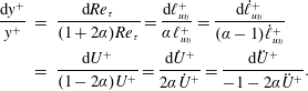 $$\begin{eqnarray}\displaystyle \frac{\text{d}y^{+}}{y^{+}} & = & \displaystyle \frac{\text{d}Re_{\unicode[STIX]{x1D70F}}}{(1+2\unicode[STIX]{x1D6FC})Re_{\unicode[STIX]{x1D70F}}}=\frac{\text{d}\ell _{uv}^{+}}{\unicode[STIX]{x1D6FC}\ell _{uv}^{+}}=\frac{\text{d}\dot{\ell }_{uv}^{+}}{(\unicode[STIX]{x1D6FC}-1)\dot{\ell }_{uv}^{+}}\nonumber\\ \displaystyle & = & \displaystyle \frac{\text{d}U^{+}}{(1-2\unicode[STIX]{x1D6FC})U^{+}}=\frac{\text{d}\dot{U}^{+}}{2\unicode[STIX]{x1D6FC}\dot{U}^{+}}=\frac{\text{d}\ddot{U} ^{+}}{-1-2\unicode[STIX]{x1D6FC}\ddot{U} ^{+}}.\end{eqnarray}$$
Here, we introduce the prolongated infinitesimals for the gradients of mean velocity (up to second order) and of the stress length function, for example, $\unicode[STIX]{x1D702}_{\dot{\ell }_{uv}^{+}}=(\unicode[STIX]{x1D6FC}-1)\dot{\ell _{uv}^{+}}$
, where
$\unicode[STIX]{x1D702}_{\dot{\ell }_{uv}^{+}}=(\unicode[STIX]{x1D6FC}-1)\dot{\ell _{uv}^{+}}$
, where $\cdot$
denotes a derivative operator in
$\cdot$
denotes a derivative operator in $y^{+}$
. The solutions to (A 9) define the following group invariants:
$y^{+}$
. The solutions to (A 9) define the following group invariants:
 $$\begin{eqnarray}\left.\begin{array}{@{}c@{}}I_{0}=Re_{\unicode[STIX]{x1D70F}}/y^{+(1+2\unicode[STIX]{x1D6FC})},\quad I_{1}=\ell _{uv}^{+}/y^{+\unicode[STIX]{x1D6FC}},\quad I_{2}=\dot{\ell }_{uv}^{+}/y^{+(\unicode[STIX]{x1D6FC}-1)},\\ G_{1}=U^{+}/y^{+(1-2\unicode[STIX]{x1D6FC})},\quad G_{2}=\dot{U}^{+}y^{+2\unicode[STIX]{x1D6FC}},\quad G_{3}=\ddot{U} ^{+}y^{+(1+2\unicode[STIX]{x1D6FC})}.\end{array}\right\}\end{eqnarray}$$
These group invariants, in general, functions of $y^{+}$
and
$y^{+}$
and $Re_{\unicode[STIX]{x1D70F}}$
, are the similarity variables (Cantwell Reference Cantwell2002).
$Re_{\unicode[STIX]{x1D70F}}$
, are the similarity variables (Cantwell Reference Cantwell2002).
Finally, in step three, we rewrite $\mathbb{C}=0$
in terms of the group invariants,
$\mathbb{C}=0$
in terms of the group invariants,
 $$\begin{eqnarray}\mathbb{C}=G_{3}+2I_{1}^{2}G_{2}G_{3}+2I_{1}I_{2}G_{2}^{2}+1/I_{0}=0.\end{eqnarray}$$
Similarly, for the outer flow, the analysis above yields (in centre units)
 $$\begin{eqnarray}\left.\begin{array}{@{}c@{}}I_{0}=Re_{\unicode[STIX]{x1D70F}}r^{1/2+\unicode[STIX]{x1D6FC}},\quad I_{1}=\ell _{uv}^{\wedge }/r^{\unicode[STIX]{x1D6FC}},\quad I_{2}=\dot{\ell }_{uv}^{\wedge }/r^{\unicode[STIX]{x1D6FC}-1},\\ G_{1}=(U_{c}^{+}-U^{+})/r^{3/2-\unicode[STIX]{x1D6FC}},\quad G_{2}=\dot{U}^{+}/r^{5/2-\unicode[STIX]{x1D6FC}},\quad G_{3}=\ddot{U} ^{+}/r^{7/2-\unicode[STIX]{x1D6FC}},\end{array}\right\}\end{eqnarray}$$
where $\cdot$
denotes
$\cdot$
denotes $r$
-derivative and the outer mean-momentum equation in terms of group invariants is
$r$
-derivative and the outer mean-momentum equation in terms of group invariants is
 $$\begin{eqnarray}\mathbb{N}=-G_{3}/I_{0}+2I_{1}^{2}G_{2}G_{3}+2I_{1}I_{2}G_{2}^{2}-1=0.\end{eqnarray}$$
Geometrically speaking, $\mathbb{C}=0$
(or
$\mathbb{C}=0$
(or $\mathbb{N}=0$
) defines an invariant surface in the variable space of
$\mathbb{N}=0$
) defines an invariant surface in the variable space of $\boldsymbol{t}$
and
$\boldsymbol{t}$
and $\boldsymbol{x}$
, which is invariant under a dilatation group of transformation, and the infinitesimals are tangent vectors to the invariant surface. The so-called invariant solution, for example,
$\boldsymbol{x}$
, which is invariant under a dilatation group of transformation, and the infinitesimals are tangent vectors to the invariant surface. The so-called invariant solution, for example, $\unicode[STIX]{x1D6E9}(\boldsymbol{t},\boldsymbol{x})=0$
, defined to satisfy the invariant surface condition, i.e.
$\unicode[STIX]{x1D6E9}(\boldsymbol{t},\boldsymbol{x})=0$
, defined to satisfy the invariant surface condition, i.e. $X\unicode[STIX]{x1D6E9}|_{\unicode[STIX]{x1D6E9}=0}=0$
, must be a function of similarity variables. The present work seeks an analytical form of the invariants of the stress length function and its first derivative, namely
$X\unicode[STIX]{x1D6E9}|_{\unicode[STIX]{x1D6E9}=0}=0$
, must be a function of similarity variables. The present work seeks an analytical form of the invariants of the stress length function and its first derivative, namely $\unicode[STIX]{x1D6E9}(I_{1},I_{2})=0$
, which is a sub-space tangent to a prescribed set of infinitesimals (e.g.
$\unicode[STIX]{x1D6E9}(I_{1},I_{2})=0$
, which is a sub-space tangent to a prescribed set of infinitesimals (e.g. $\unicode[STIX]{x1D709}_{y^{+}}$
,
$\unicode[STIX]{x1D709}_{y^{+}}$
, $\unicode[STIX]{x1D702}_{\ell _{uv}^{+}}$
and
$\unicode[STIX]{x1D702}_{\ell _{uv}^{+}}$
and $\unicode[STIX]{x1D702}_{\dot{\ell }_{uv}^{+}}$
).
$\unicode[STIX]{x1D702}_{\dot{\ell }_{uv}^{+}}$
).
Appendix B. The structure ensemble dynamics theory
The structure ensemble dynamics (SED) theory aims to develop a foundation dealing with the (statistical) symmetry of turbulence (Frisch Reference Frisch1995), based on which a quantitative description becomes feasible. It originates from three concepts, i.e. ensemble, structure and dynamics, with the following fundamental assumption: the ensemble property of structure and dynamics, spatial and temporal constituents of physical systems (e.g. wall flows), is a quantifiable behaviour governed by a statistical symmetry. Thus, to uncover the relevant statistical symmetry would be the main task to reveal the simplicity of a turbulent system, a complex system induced by various boundary conditions and nonlinear multi-scale interactions among a large number of degrees of freedom. In this section, we address why and how the SED provides a general framework to quantify wall-bounded turbulent systems.
Dilation symmetry is of particular importance to turbulent wall flows due to the constraint by the presence of wall. The non-slip wall condition governs all terms in the RANS equations (including mean-momentum, kinetic-energy and internal-energy equations) when any transformations are performed. SED, following Landau’s spirit, further assumes that the dilatation symmetry also determines the solutions of RANS equations (i.e. distributions of mean quantities) through order parameter/function which describes ensemble properties emerged from the turbulence fluctuation background. The relevant order parameter/function, once identified, is thus the key to quantifying turbulence, since its role of symmetry is universal to wall flows. Specifically, SED theory involves two important concepts, i.e. multi-state and order function, which are universal to all wall flows as explained in detail below.
B.1 Multi-state symmetries with distinct energy-balance mechanism
Turbulence as a typical non-equilibrium process displays a number of symmetry-breaking behaviours. In wall-bounded flows, when turbulent fluctuations arise, several balance mechanisms in energy dynamics (e.g. turbulence production or transport-balance dissipation) are comparable, which is the origin of different scaling of stress length. Thus, it is natural to conjecture that multi-state is the general form of symmetry-breaking in wall turbulence. To facilitate the generalization of the present analysis to other flows, a basic set of postulates are formulated as follows: (i) the existence of wall introduces a finite number of statistical states due to the presence of different characteristic fluctuation structures; (ii) each state covers a spatially extended domain, which is a layer in wall-bounded flows, depending on the distance from the wall; and (iii) layers, as well as transitions between layers, are characterized by the symmetry properties of the order functions. In other words, wall-bounded turbulent flows typically exhibit a ‘multi-layer structure’. Then, the key issue is to find appropriate variables and suitable formalisms for their descriptions; this is accomplished by the concept of order function as described below.
B.2 Order function
Generally speaking, order functions are quantities displaying distinct symmetry properties. It is inspired by the concept of order parameter in the statistical mean-field theory, which describes the changes of the statistical state (e.g. phase transition) associated with symmetry breaking. In critical phenomena, phase transition accompanies symmetry changes, which alter the scaling exponent. In turbulent flow, fluctuations inherently alter the mean velocity (through Reynolds stress) and this interaction also constitutes symmetry breaking. This effect is described by introducing a length order function, which displays a distinct character from one layer to another by its dilatation-invariant scaling. In a sense, turbulent fluctuations restore a dilatation symmetry (layer by layer) (Frisch Reference Frisch1995) and the symmetry property can be quantified by the scaling of the order functions.
An order function typically involves a ratio of two (or more) statistical quantities. Finding an appropriate order function for a given turbulent flow is the very first step in a SED study of turbulent flows. Three kinds of order functions have been suggested (She et al. Reference She, Chen, Wu and Hussain2010). The first is a ratio between two (dominant) terms in the governing equation (mean-momentum equation or mean kinetic-energy equation), called ratio-order function. The ratio-order function is particularly effective in connecting the statistical state to its dynamical origin, e.g. linking the multi-layer to the balance mechanism in the momentum or energy equation. The second is a length function, which is probably the most important quantity for describing physics phenomena; the complexity of turbulence lies in the fact that multiple characteristic length scales are relevant to different aspects of turbulence dynamics. Usually, dimensional argument is sufficient to define a number of relevant length scales (such as the stress length function). The third is a sensitive indicator function with correct (theoretical) asymptotic scaling which is effective to incorporate boundary effects and can be used to check the quality of simulation (see She et al. Reference She, Chen, Wu and Hussain2010).
Note that we keep the list of order function open, as additional fluctuations (such as density, temperature, etc.) may introduce new order functions. As more flows are studied by us, we will show that for each flow, there always exists a set of order functions which exhibit distinct symmetry behaviour across different layers and hold important physical constants – some of which (like Karman constant) maybe universal for different kinds of flows.
B.3 How does one proceed in a SED study of turbulence?
A SED study of turbulence proceeds in three steps. First, it consists in verifying the existence of the symmetry, which amounts to verifying whether the order function has local scaling. Second, it determines the parameters, such as scaling exponents and layer thicknesses, with available empirical data. In particular, one would identify universal constants which do not vary with physical conditions ( $Re$
,
$Re$
, $Ma$
, geometry, surface roughness, pressure gradient, etc.). Finally, based on the above qualitative (first step) and quantitative (second step) information, one calculates important quantities (such as friction coefficient, heat flux, etc.) in the third step, for making predictions for a range of physical parameters (such as
$Ma$
, geometry, surface roughness, pressure gradient, etc.). Finally, based on the above qualitative (first step) and quantitative (second step) information, one calculates important quantities (such as friction coefficient, heat flux, etc.) in the third step, for making predictions for a range of physical parameters (such as $Re$
,
$Re$
, $Ma$
, etc.). The three steps constitute a complete procedure, going from DNS analysis to relevant engineering model construction (as we have done for improving the
$Ma$
, etc.). The three steps constitute a complete procedure, going from DNS analysis to relevant engineering model construction (as we have done for improving the $k{-}\unicode[STIX]{x1D714}$
model Chen et al.
Reference Chen, Hussain and She2016a
). Note that this procedure is also applicable to a number of wall flows under a variety of physical conditions (such as two-phase flows, magneto-hydrodynamic flow, flows in tokamac, etc.), which can be helpful in better utilizing a DNS study of practical flow systems. The SED is proposed to fulfil this need.
$k{-}\unicode[STIX]{x1D714}$
model Chen et al.
Reference Chen, Hussain and She2016a
). Note that this procedure is also applicable to a number of wall flows under a variety of physical conditions (such as two-phase flows, magneto-hydrodynamic flow, flows in tokamac, etc.), which can be helpful in better utilizing a DNS study of practical flow systems. The SED is proposed to fulfil this need.


 Open access

