


1. Introduction
Rapid advances in micro-fabrication techniques have aided the miniaturisation and integration of electro-mechanical systems on tiny chips. These micro-electro-mechanical systems find applications in areas ranging from biomedical devices to micro space/aerial vehicles. Currently, these devices rely on low-energy density batteries for their power requirements, which limits their portability and functionality. Micro/meso combustors were initially conceived as potential alternatives to power these devices since the energy density of a typical liquid hydrocarbon is two orders higher in magnitude than standard alkaline/Li-ion batteries (Fernandez-Pello Reference Fernandez-Pello2002; Maruta Reference Maruta2011; Kaisare & Vlachos Reference Kaisare and Vlachos2012). However, micro/meso-scale combustion has found its way into other domains in the form of micro-reactors (that find extensive applications in quantitative chemistry as reported by Zimmermann et al. (Reference Zimmermann, Krippner, Vogel and Müller2002)) and fire safety systems. In this context, ‘micro’ describes combustors with a characteristic length scale smaller than the quenching diameter, while ‘meso’ combustors have a larger length scale that is of the order of the quenching diameter (Ju & Maruta Reference Ju and Maruta2011).
When the combustor size drops to micro or meso scales, the surface area-to-volume ratio increases significantly. As a result, wall heat losses become a critical factor, making the flame susceptible to both thermal and radical quenching. To sustain combustion under these conditions, a widely adopted strategy involves the upstream recirculation of heat from the product gases into the unburnt reactants. This approach preheats the reactants and alters the temperature gradient at the walls, thereby mitigating heat losses and enabling the flame to persist in channels narrower than the classical quenching limit (Lloyd & Weinberg Reference Lloyd and Weinberg1974). Unlike large-scale combustors, where the walls primarily act as a sink for heat and radicals, flame--wall interactions at smaller scales are more complex. In micro and meso combustors, the walls can also contribute energy to the fluid, depending on the Biot and Fourier numbers. This intricate coupling between the flame and the walls can give rise to additional flame regimes that are not observed in large-scale systems. Evans & Kyritsis (Reference Evans and Kyritsis2011) demonstrated that the thermal properties of the walls, especially thermal conductivity, significantly influence the temperature distribution along the walls and the overall flame dynamics in micro and meso combustors. Recent advancements, such as segmented nozzle designs (Luo et al. Reference Luo, Jiaqiang, Chen, Zhang and Ding2024), have significantly improved wall temperature distribution, thereby enhancing the stability and efficiency of micro-scale flames. Furthermore, the incorporation of innovative features like conical rings has been shown to effectively enhance flame stability (Cai et al. Reference Cai, Jiaqiang, Zhao and Zhao2024; Li et al. Reference Li, Jiaqiang, Ding, Cai and Luo2024). The following discussion explores the commonly observed flame behaviours at these small scales, shedding light on the unique dynamics that arise in micro and meso combustors.
Maruta et al. (Reference Maruta, Parc, Oh, Fujimori, Minaev and Fursenko2004, Reference Maruta, Kataoka, Kim, Minaev and Fursenko2005) conducted studies with a cylindrical quartz tube of inner diameter $2\,\rm mm$
that acts as an optically accessible micro combustor for premixed methane--air flames. The effect of product gas heat recirculation was imposed using two heating plates positioned at the top and bottom of the tube. In addition to the stationary flames (SFs) that establish themselves at a specific section within the channel, various unsteady flame behaviours were also documented. These included a flame exhibiting a series of ignition, propagation, extinction and re-ignition events, referred to as flames with repetitive extinction and ignition (FREI), as well as a pulsating flame and a flame displaying traits of both pulsation and FREI. Similar observations were reported by Fan et al. (Reference Fan, Minaev, Sereshchenko, Fursenko, Kumar, Liu and Maruta2009) in premixed methane--air flames inside micro-scale rectangular quartz channels of different cross-sections. Ju & Xu (Reference Ju and Xu2005) conducted both theoretical and experimental studies on the propagation and extinction of flames at meso scales. Their findings indicate that a flame within a meso-scale channel could propagate at velocities exceeding that of an adiabatic flame, contingent upon the thermal characteristics and heat capacity of the channel walls. Moreover, in addition to heat recirculation from the product gases, streamwise heat conduction along the walls from the flame can also elevate the temperature of the reactant mixture upstream of the flame front, as noted by Kessler & Short (Reference Kessler and Short2008). This upstream heating has a direct impact on the flame speed, further illustrating the complex interplay between thermal processes and flame dynamics in meso-scale systems.
$2\,\rm mm$
that acts as an optically accessible micro combustor for premixed methane--air flames. The effect of product gas heat recirculation was imposed using two heating plates positioned at the top and bottom of the tube. In addition to the stationary flames (SFs) that establish themselves at a specific section within the channel, various unsteady flame behaviours were also documented. These included a flame exhibiting a series of ignition, propagation, extinction and re-ignition events, referred to as flames with repetitive extinction and ignition (FREI), as well as a pulsating flame and a flame displaying traits of both pulsation and FREI. Similar observations were reported by Fan et al. (Reference Fan, Minaev, Sereshchenko, Fursenko, Kumar, Liu and Maruta2009) in premixed methane--air flames inside micro-scale rectangular quartz channels of different cross-sections. Ju & Xu (Reference Ju and Xu2005) conducted both theoretical and experimental studies on the propagation and extinction of flames at meso scales. Their findings indicate that a flame within a meso-scale channel could propagate at velocities exceeding that of an adiabatic flame, contingent upon the thermal characteristics and heat capacity of the channel walls. Moreover, in addition to heat recirculation from the product gases, streamwise heat conduction along the walls from the flame can also elevate the temperature of the reactant mixture upstream of the flame front, as noted by Kessler & Short (Reference Kessler and Short2008). This upstream heating has a direct impact on the flame speed, further illustrating the complex interplay between thermal processes and flame dynamics in meso-scale systems.
Jackson et al. (Reference Jackson, Buckmaster, Lu, Kyritsis and Massa2007) compared the problem of flame propagation/stabilisation in narrow ducts to that of an edge flame and proposed a model that captured the transition between steady and unsteady flame solutions. The model only had thermal considerations and ignored hydrodynamic contributions by directly imposing a Poiseuille velocity profile inside the duct. This treatment was further emphasised by Bieri et al. (Reference Bieri, Kurdyumov and Matalon2011) and Evans & Kyritsis (Reference Evans and Kyritsis2011). Nonetheless, it was observed that the frequency of flame oscillations in unsteady flames aligned with the Strouhal number associated with the instability of the jet emerging from the micro/meso channels (St $\sim$
0.4; Richecoeur & Kyritsis Reference Richecoeur and Kyritsis2005), emphasising the role of hydrodynamics in dictating the quantitative flame dynamics. Flame--wall interactions in unsteady flame regimes was extensively studied by Evans & Kyritsis (Reference Evans and Kyritsis2009, Reference Evans and Kyritsis2011). Their work showed that a thin wall serves a dual purpose: acting as a heat sink following ignition, resulting in flame extinction due to rapid heat losses, as well as enabling re-ignition since the wall temperature rises quickly (due to flame–wall interaction) due to the associated low thermal inertia. Consequently, this leads to high-frequency extinction and re-ignition events (FREI).
$\sim$
0.4; Richecoeur & Kyritsis Reference Richecoeur and Kyritsis2005), emphasising the role of hydrodynamics in dictating the quantitative flame dynamics. Flame--wall interactions in unsteady flame regimes was extensively studied by Evans & Kyritsis (Reference Evans and Kyritsis2009, Reference Evans and Kyritsis2011). Their work showed that a thin wall serves a dual purpose: acting as a heat sink following ignition, resulting in flame extinction due to rapid heat losses, as well as enabling re-ignition since the wall temperature rises quickly (due to flame–wall interaction) due to the associated low thermal inertia. Consequently, this leads to high-frequency extinction and re-ignition events (FREI).
Studies by Richecoeur & Kyritsis (Reference Richecoeur and Kyritsis2005) and David P (Reference David2012) have also documented acoustic emissions from flames in the FREI regime. Their research indicates that these acoustic signals correspond to gas expansion events (pressure bursts) occurring during the ignition phase of unsteady flames. The associated frequency spectrum was found to span a wide range, including the natural harmonic modes of the combustor. However, the amplitude of these pressure fluctuations decays to quiescent levels as the flame propagates upstream following ignition. David (Reference David2012) emphasised that the level of acoustic emissions depends significantly on the specific experimental set-up. Their studies demonstrated that sound generation– or its absence– is heavily influenced by the thermal conductivity of the combustor’s wall material; higher conductivity amplifies sound emissions.
Recent studies by Tang et al. (Reference Tang, Cai, Li, Zhou and Gao2024) and Cai et al. (Reference Cai, Tang, Zhao, Zhou and Huang2020) also report acoustic emissions in oscillating flame regimes. These flames exhibited fluctuations in the flame front and were localised to a region inside the combustor without upstream propagation (unlike FREI). The observed pressure fluctuations were found to correspond to the oscillations of the flame front. However, the frequencies of these fluctuations were significantly off from the natural harmonic of the combustor tube. Similarly, studies by Prakash et al. (Reference Prakash, Armijo, Masel and Shannon2007a ,Reference Prakash, Armijo, Masel and Shannonb ) on the dynamics of non-premixed methane–oxygen flames in micro-scale channels demonstrated acoustic emissions during the transient phase preceding the establishment of a steady-state flame. In this phase, an edge flame with an elongated tail was observed to anchor at the inlet of the mixing layer between the methane–oxygen streams. Additionally, an unsteady flame undergoing repetitive cycles of ignition and extinction was present. The corresponding acoustic signals exhibited two dominant peaks: one associated with the repetition frequency of the unsteady flame and the other near the natural harmonic of the combustor tube. The authors hypothesised that the second peak is thermoacoustic in nature and attributed it to the steady flame anchored at the mixing layer. However, the acoustic emission ceased to exist beyond the transient phase. Interestingly, thermoacoustic coupling, which is widely observed in large-scale combustors (Schuller et al. Reference Schuller, Poinsot and Candel2020; Mohan & Mariappan Reference Mohan and Mariappan2023) and flames propagating inside channels (Castela et al. Reference Castela, Correa, Alam, Jason and Lacoste2021; Dubey et al. Reference Dubey, Koyama, Hashimoto and Fujita2021; Flores-Montoya et al. Reference Flores-Montoya, Muntean, Pozo-Estivariz and Martínez-Ruiz2023), has not been reported in periodically repeating unsteady flame regimes within micro/meso-scale combustors. This phenomenon will be discussed further in the current work, wherein we report a novel periodically repeating unsteady flame regime exhibiting thermoacoustic coupling while traversing to the upstream end of the tube.
Studies have also explored the micro/meso channel flame dynamics under different wall temperature profiles (all the investigated temperature profiles are monotonic along the combustor axis). Kang et al. (Reference Kang, Gollan, Jacobs and Veeraragavan2017) performed numerical investigations on methane–air flames in microchannels, revealing that flame propagation speed depends not only on the chemical heat release rate but also on the rate of heat exchange between the flame and the channel walls. These interactions collectively result in quantitative variations in flame regime characteristics under different wall temperature profiles. Similarly, Ratna Kishore et al. (Reference Ratna Kishore, Minaev, Akram and Kumar2017) demonstrated that reducing the axial wall temperature gradients shifts the ignition location toward zones with lower wall temperatures. Numerical studies by Wang and collaborators (Wang & Fan Reference Wang and Fan2021a ,Reference Wang and Fanb , Reference Wang and Fan2022, Reference Wang and Fan2023; Liu et al. Reference Liu, Wang and Fan2025) have highlighted the significant impact of wall temperature profiles on micro-scale flame dynamics. Their research reveals a variety of complex phenomena, including the coexistence of upstream normal and downstream weak flames, FREI exhibiting multiple bifurcations and other intricate flame behaviours driven by incomplete combustion and residual species. Notably, variations in wall temperature gradients and profiles were shown to play a pivotal role in influencing flame stability, flame structure and reaction pathways. These findings underscore that changes in wall temperature distributions are critical for controlling and predicting flame behaviour in micro- and meso-scale combustion systems.
In practical meso-scale combustors such as swiss-roll burners, where combustion is stabilised at the centre, hot product gases follow a rectangular outward spiral path while reactants travel along an inward rectangular spiral path to reach the reaction-stabilised centre of the combustor. The wall temperature profile is expected to decrease monotonically as we move radially outward from the reaction zone. However, as the flow decelerates at the corners of these rectangular spiral paths, regions with minor spikes in the wall temperature profile are anticipated. The existing literature provides compelling evidence to show that such spikes in the wall temperature profile can significantly influence flame–wall interactions, leading to both quantitative and qualitative changes in flame dynamics. A simplified depiction of wall temperature spikes causing changes in the flame behaviour is discussed in the current study.
The objective of the current study is twofold. The first part investigates the dynamics of unsteady premixed methane–air flames in meso-scale channels, imposed with a monotonically decaying temperature profile along the combustor axis (in the upstream direction). Alongside the well-documented FREI regime, we report the observation of a periodically repeating unsteady novel flame regime that exhibits thermoacoustic coupling. Additionally, we explore the changes in the dynamics of these unsteady flame regimes following the imposition of a bimodal heating profile. This bimodal profile represents a simplified one-dimensional depiction of the local temperature spike imposed over a monotonically decaying wall temperature profile along the combustor axis.
2. Experimental set-up
2.1. Meso-scale combustor facility
A cylindrical quartz channel of $5\,\rm mm$
inner diameter (
$5\,\rm mm$
inner diameter ( ${d}_{i}$
) and
${d}_{i}$
) and $7\,\rm mm$
outer diameter (
$7\,\rm mm$
outer diameter ( $d_{o}$
) is used as an optically accessible meso-scale combustor (length:
$d_{o}$
) is used as an optically accessible meso-scale combustor (length: $380\,\rm mm$
). The channel is heated using two external heaters: a primary heater and a secondary heater, as depicted in figure 1(a). The primary heating unit consists of two heating torches, each fitted with
$380\,\rm mm$
). The channel is heated using two external heaters: a primary heater and a secondary heater, as depicted in figure 1(a). The primary heating unit consists of two heating torches, each fitted with $12\,\rm mm$
cylindrical nozzles at their tips. These torches are oriented at an angle of
$12\,\rm mm$
cylindrical nozzles at their tips. These torches are oriented at an angle of $35^{\circ}$
from the central plane (as shown in figure 1a, right) such that the combustor tube passes through the stagnation plane of the jet flames produced by the torches. The tips of the torches are positioned
$35^{\circ}$
from the central plane (as shown in figure 1a, right) such that the combustor tube passes through the stagnation plane of the jet flames produced by the torches. The tips of the torches are positioned $20\,\rm mm$
below the axis of the combustor tube. The secondary heater is a McKenna flat flame burner, featuring a flat, circular porous surface with a diameter of
$20\,\rm mm$
below the axis of the combustor tube. The secondary heater is a McKenna flat flame burner, featuring a flat, circular porous surface with a diameter of $60\,\rm mm$
at the top, over which a flat flame is stabilised. It is positioned
$60\,\rm mm$
at the top, over which a flat flame is stabilised. It is positioned $25\,\rm mm$
below the combustor tube axis. The dual-torch primary heater directs the flame onto a narrow section of the combustor tube, with a width approximately matching the nozzle diameter (
$25\,\rm mm$
below the combustor tube axis. The dual-torch primary heater directs the flame onto a narrow section of the combustor tube, with a width approximately matching the nozzle diameter ( $12\,\rm mm$
). In contrast, the secondary heater heats a broader section of the tube, corresponding to the
$12\,\rm mm$
). In contrast, the secondary heater heats a broader section of the tube, corresponding to the $60\,\rm mm$
diameter of its porous surface. This distinction is clear in figure 1(b), which plots the inner wall temperature profile along the combustor axis. The figure shows that the primary heating zone (the combustor section directly above the primary heater) is narrower compared with the secondary heating zone (the section above the secondary heater). Additionally, the peak temperature in the primary heating zone (
$60\,\rm mm$
diameter of its porous surface. This distinction is clear in figure 1(b), which plots the inner wall temperature profile along the combustor axis. The figure shows that the primary heating zone (the combustor section directly above the primary heater) is narrower compared with the secondary heating zone (the section above the secondary heater). Additionally, the peak temperature in the primary heating zone ( ${\sim }1130\,\rm K$
) is higher than that in the secondary heating zone (
${\sim }1130\,\rm K$
) is higher than that in the secondary heating zone ( ${\sim}1025\,\rm K$
) and is a result of positioning the primary heater closer to the combustor axis than the secondary heater. In combination, the primary and secondary heaters impose a bimodal wall heating profile over the combustor walls. The distance between the centres of the heaters, characterised by
${\sim}1025\,\rm K$
) and is a result of positioning the primary heater closer to the combustor axis than the secondary heater. In combination, the primary and secondary heaters impose a bimodal wall heating profile over the combustor walls. The distance between the centres of the heaters, characterised by $d$
(figure 1a), is varied to obtain different bimodal wall heating profiles. The secondary heater was intentionally positioned farther from the combustor tube axis (than the primary heater) to ensure that it only preheats the premixed reactant mixture without triggering an auto-ignition event. In contrast, the primary heater was specifically designed to induce auto-ignition of the reactant mixture.
$d$
(figure 1a), is varied to obtain different bimodal wall heating profiles. The secondary heater was intentionally positioned farther from the combustor tube axis (than the primary heater) to ensure that it only preheats the premixed reactant mixture without triggering an auto-ignition event. In contrast, the primary heater was specifically designed to induce auto-ignition of the reactant mixture.
(a) Experimental set-up. (b) Inner wall temperature profiles at different separation distances ( $d/{d}_{i}$
). The regions highlighted in brown and yellow represent the primary and secondary heating zones, respectively, for
$d/{d}_{i}$
). The regions highlighted in brown and yellow represent the primary and secondary heating zones, respectively, for $d/{d}_{i}=18$
.
$d/{d}_{i}=18$
.

Figure 1(b) depicts the spatial profile of the wall temperature measured along the inner walls of the combustor tube, using a $1\,\rm mm$
K-type thermocouple. It is to be noted that since the combustor tube is heated from below, the inner wall temperature is not uniform across the combustor cross-section. The lower periphery, in closer proximity to the heaters, has a higher wall temperature compared with the upper periphery. This disparity was most pronounced in the primary heating zone, reaching approximately
$1\,\rm mm$
K-type thermocouple. It is to be noted that since the combustor tube is heated from below, the inner wall temperature is not uniform across the combustor cross-section. The lower periphery, in closer proximity to the heaters, has a higher wall temperature compared with the upper periphery. This disparity was most pronounced in the primary heating zone, reaching approximately $2\,\%$
of the measured temperature. The temperature profiles depicted in figure 1(b) represent inner wall temperature measured along the lower periphery of the combustor in the axial direction. A plot comparing the inner wall temperatures along the lower and upper peripheries is provided in section S1 of the supplementary material. The profiles are estimated from three sets of experimental measurements and correspond to quiescent conditions inside the combustor.
$2\,\%$
of the measured temperature. The temperature profiles depicted in figure 1(b) represent inner wall temperature measured along the lower periphery of the combustor in the axial direction. A plot comparing the inner wall temperatures along the lower and upper peripheries is provided in section S1 of the supplementary material. The profiles are estimated from three sets of experimental measurements and correspond to quiescent conditions inside the combustor.
Methane and air regulated through two precise mass flow controllers (Bronkhorst flexi-flow compact with the range of 0–1.6 SLPM for $\rm CH_4$
and 0–2 SLPM for air) are directed into a mixing chamber, where the streams mix into each other to create a homogeneous mixture, which is then subsequently fed into the quartz combustor tube at its upstream end. The flow rates of liquefied petroleum gas and air into the primary and secondary heaters were controlled using precise pressure regulators and mass flow controllers (Alicat Scientific MCR-500SLPM), respectively. In the discussions that follow, the
$\rm CH_4$
and 0–2 SLPM for air) are directed into a mixing chamber, where the streams mix into each other to create a homogeneous mixture, which is then subsequently fed into the quartz combustor tube at its upstream end. The flow rates of liquefied petroleum gas and air into the primary and secondary heaters were controlled using precise pressure regulators and mass flow controllers (Alicat Scientific MCR-500SLPM), respectively. In the discussions that follow, the $x$
axis is oriented along the combustor axis, extending along the downstream direction. The origin (
$x$
axis is oriented along the combustor axis, extending along the downstream direction. The origin ( $x=0\,\rm mm$
) is set at the upstream end of the tube. The quartz tube connects to the upstream mixing chamber via a
$x=0\,\rm mm$
) is set at the upstream end of the tube. The quartz tube connects to the upstream mixing chamber via a $1.5$
mm tubular constriction followed by a flashback arrestor. The
$1.5$
mm tubular constriction followed by a flashback arrestor. The $1.5\,\rm mm$
tube houses a
$1.5\,\rm mm$
tube houses a $100\,\unicode{x03BC}\rm m$
wire mesh upstream of
$100\,\unicode{x03BC}\rm m$
wire mesh upstream of $x=0\,\rm mm$
.
$x=0\,\rm mm$
.
The current study was performed at three different equivalence ratios ( $\Phi$
):
$\Phi$
): $0.8$
,
$0.8$
, $1.0$
and
$1.0$
and $1.2$
. The mixture velocity (
$1.2$
. The mixture velocity ( $\bar {u}$
) was varied between
$\bar {u}$
) was varied between $0.1$
and
$0.1$
and $0.3\,\rm m\,s^-{^1}$
in increments of
$0.3\,\rm m\,s^-{^1}$
in increments of $0.05\,\rm m\,s^-{^1}$
, yielding upstream Reynolds numbers between
$0.05\,\rm m\,s^-{^1}$
, yielding upstream Reynolds numbers between $32$
and
$32$
and $96$
in increments of
$96$
in increments of $16$
. The experiments were conducted with four different wall heating conditions: a baseline case, wherein only the primary heater was used (no flat flame burner), and three other cases, wherein the distance between the centres of the dual torch and the flat flame burner (
$16$
. The experiments were conducted with four different wall heating conditions: a baseline case, wherein only the primary heater was used (no flat flame burner), and three other cases, wherein the distance between the centres of the dual torch and the flat flame burner ( $d$
) was varied between
$d$
) was varied between $75\,\rm mm$
to
$75\,\rm mm$
to $105\,\rm mm$
, in increments of
$105\,\rm mm$
, in increments of $15\,\rm mm$
, which corresponds to
$15\,\rm mm$
, which corresponds to $d/d_{i}$
of
$d/d_{i}$
of $15$
,
$15$
, $18$
and
$18$
and $21$
. The axial temperature profile corresponding to these cases is plotted in figure 1(b).
$21$
. The axial temperature profile corresponding to these cases is plotted in figure 1(b).
2.2. High-speed flame imaging and data acquisition from PMT and microphone
A Phantom Miro Lab 110 high-speed camera coupled with a $100\,\rm mm$
Tokina macro-lens was used for high-speed flame imaging. The dynamics were captured at 4000 frames per second (
$100\,\rm mm$
Tokina macro-lens was used for high-speed flame imaging. The dynamics were captured at 4000 frames per second ( $250\,\unicode{x03BC}\rm s$
exposure time) with a spatial resolution of
$250\,\unicode{x03BC}\rm s$
exposure time) with a spatial resolution of $200\,\unicode{x03BC}\rm m$
per pixel (frame size of 1280 × 120 pixels). The data were used to track the spatial location of the flame. It is to be noted that the initial
$200\,\unicode{x03BC}\rm m$
per pixel (frame size of 1280 × 120 pixels). The data were used to track the spatial location of the flame. It is to be noted that the initial $65\,\rm mm$
segment of the quartz tube was inaccessible for imaging due to the presence of a steel support that held the
$65\,\rm mm$
segment of the quartz tube was inaccessible for imaging due to the presence of a steel support that held the $380\,\rm mm$
long quartz combustor tube in the form of a cantilever (figure 1a). The OH* chemiluminescence signal of the flame was captured using a Hamamatsu photomultiplier tube (PMT, H 11526-110-NF). The PMT was positioned at a distance of
$380\,\rm mm$
long quartz combustor tube in the form of a cantilever (figure 1a). The OH* chemiluminescence signal of the flame was captured using a Hamamatsu photomultiplier tube (PMT, H 11526-110-NF). The PMT was positioned at a distance of $70\,\rm mm$
from the downstream end of the combustor along the tube axis, such that the photocathode is exposed to the flame inside the combustor tube via a Nikon Rayfact (PF10445MF) UV lens and an OH* bandpass filter (
$70\,\rm mm$
from the downstream end of the combustor along the tube axis, such that the photocathode is exposed to the flame inside the combustor tube via a Nikon Rayfact (PF10445MF) UV lens and an OH* bandpass filter ( $\sim 310 \pm 10\,\text {nm}$
); depicted in figure 1(a). The pressure field fluctuation was recorded using a PCB microphone (PCB 130E20), which was placed at a radial distance of
$\sim 310 \pm 10\,\text {nm}$
); depicted in figure 1(a). The pressure field fluctuation was recorded using a PCB microphone (PCB 130E20), which was placed at a radial distance of $80\,\rm mm$
from the combustor axis at the downstream end of the combustor tube (figure 1a). The data from the PMT and the microphone were acquired using an NI-DAQ (PCI 6251) at 12,000 Hz and was triggered alongside flame imaging via the high-speed camera.
$80\,\rm mm$
from the combustor axis at the downstream end of the combustor tube (figure 1a). The data from the PMT and the microphone were acquired using an NI-DAQ (PCI 6251) at 12,000 Hz and was triggered alongside flame imaging via the high-speed camera.
The flame images from the high-speed camera were processed in ImageJ, where they were subjected to thresholding using the Otsu thresholding technique, an integral feature of ImageJ. Otsu’s thresholding algorithm calculates a single intensity threshold value ( $I_f$
) that separates all the pixels within an image into two categories: foreground and background. This threshold value
$I_f$
) that separates all the pixels within an image into two categories: foreground and background. This threshold value $(I_f)$
is determined by minimising the variance within each category or maximising the variance between the two. Pixels
$(I_f)$
is determined by minimising the variance within each category or maximising the variance between the two. Pixels $(i, j)$
with intensities greater than or equal to
$(i, j)$
with intensities greater than or equal to $I_f$
are set to a binary value of 1, while those with intensities less than
$I_f$
are set to a binary value of 1, while those with intensities less than $I_f$
are assigned 0. The resulting binary area, comprising pixels with a value of 1, delineates the flame’s boundary. Once the boundary is estimated, the location of the flame (
$I_f$
are assigned 0. The resulting binary area, comprising pixels with a value of 1, delineates the flame’s boundary. Once the boundary is estimated, the location of the flame ( $x_f$
) is tracked by estimating the centroid of the region isolated by the flame boundary. The method has proven to be an effective technique for tracking the position of the flame and has been implemented previously by Vadlamudi et al. (Reference Vadlamudi, Thirumalaikumaran and Basu2021), Pandey et al. (Reference Pandey, Basu, Gautham, Potnis and Chattopadhyay2020), Thirumalaikumaran et al. (Reference Thirumalaikumaran, Vadlamudi and Basu2022) and Vadlamudi et al. (Reference Vadlamudi, Aravind and Basu2023). The position of the flame is tracked spatially with respect to time to obtain the flame propagation speed (
$x_f$
) is tracked by estimating the centroid of the region isolated by the flame boundary. The method has proven to be an effective technique for tracking the position of the flame and has been implemented previously by Vadlamudi et al. (Reference Vadlamudi, Thirumalaikumaran and Basu2021), Pandey et al. (Reference Pandey, Basu, Gautham, Potnis and Chattopadhyay2020), Thirumalaikumaran et al. (Reference Thirumalaikumaran, Vadlamudi and Basu2022) and Vadlamudi et al. (Reference Vadlamudi, Aravind and Basu2023). The position of the flame is tracked spatially with respect to time to obtain the flame propagation speed ( $S_f$
) in the reference frame of zero upstream mixture velocity, compensating for the relative velocity of the incoming mixture (
$S_f$
) in the reference frame of zero upstream mixture velocity, compensating for the relative velocity of the incoming mixture ( $\bar {u}$
) with respect to the upstream traversing flame. Mathematically,
$\bar {u}$
) with respect to the upstream traversing flame. Mathematically, $S_f$
can be expressed as
$S_f$
can be expressed as
 \begin{align} S_f = \frac {{\rm d}x_f}{{\rm d}t} - \bar {u} \Rightarrow \ S_f = \frac {{\rm d}x_f}{{\rm d}t} + |\bar {u}|. \end{align}
It is to be noted that in the above relation, $\bar {u}$
is the velocity of the fuel–air mixture measured along the x axis, while
$\bar {u}$
is the velocity of the fuel–air mixture measured along the x axis, while $S_f$
and
$S_f$
and ${{\rm d}x_f}/{{\rm d}t}$
are measured along the negative x axis since the flame tends to traverse upstream with respect to the incoming flow.
${{\rm d}x_f}/{{\rm d}t}$
are measured along the negative x axis since the flame tends to traverse upstream with respect to the incoming flow.
The OH* chemiluminescence and microphone signals are processed in MATLAB after filtering it using the Savitzky–Golay filter (Savitzky & Golay Reference Savitzky and Golay1964), which is a low-pass filter based on the local least-square polynomial approximation that smooths the signal without distorting it (Di Stazio et al. Reference Di Stazio, Chauveau, Dayma and Dagaut2016a ,Reference Di Stazio, Chauveau, Dayma and Dagautb ). The data from the PMT and the pressure sensor were used to estimate the time scales associated with the unsteady meso-scale flame regimes. In the discussion presented in the subsequent sections, all the descriptors of unsteady flames (position, flame propagation speeds, OH* chemiluminescence, frequency of repetition, time scales, etc.) are results averaged out over at least ten periodic repetition cycles from three different trials.
3. Results and discussion
3.1. Global observations
Premixed methane–air mixture, at $300\,\rm K$
, enters the quartz combustor tube at
$300\,\rm K$
, enters the quartz combustor tube at $x=0\,\rm mm$
and travels downstream, continuously gaining heat from the combustor walls and increasing its mean flow temperature (
$x=0\,\rm mm$
and travels downstream, continuously gaining heat from the combustor walls and increasing its mean flow temperature ( $T_m$
). The mixture auto-ignites close to the primary heating zone where the inner wall temperatures are close to
$T_m$
). The mixture auto-ignites close to the primary heating zone where the inner wall temperatures are close to $1130\,\rm K$
. Upon auto-ignition, the mixture starts to propagate upstream, consuming the incoming reactants. This behaviour is consistently observed across the space of experimental conditions explored in the current work. However, this upstream traversing flame exhibits different dynamics contingent on the operating conditions of Reynolds numbers (
$1130\,\rm K$
. Upon auto-ignition, the mixture starts to propagate upstream, consuming the incoming reactants. This behaviour is consistently observed across the space of experimental conditions explored in the current work. However, this upstream traversing flame exhibits different dynamics contingent on the operating conditions of Reynolds numbers ( $Re$
), equivalence ratios (
$Re$
), equivalence ratios ( $\Phi$
) and imposed wall heating profiles. Two global flame behaviours emerge, steady flames and unsteady flames.
$\Phi$
) and imposed wall heating profiles. Two global flame behaviours emerge, steady flames and unsteady flames.
Stationary stable flames (steady flames) stabilise themselves at a characteristic upstream location (figure 2a) post ignition. However, the unsteady flames demonstrate two distinct patterns: they either extinguish after traversing a characteristic distance (figure 2b) or persist (continue propagating) until extinguished at the upstream meshed constriction of the combustor tube (figure 2d) at $x=0\,\rm mm$
. These unsteady flame regimes demonstrate periodic recurrence, reigniting after a characteristic time delay following extinction, as the fresh incoming mixture auto-ignites and repeats the flame cycle. Accordingly, three major flame regimes can be identified: stationary flames (SF), flames with repetitive extinction and ignition (FREI) and propagating flames (PF), respectively. In the subsequent sections, the dynamics of the latter-mentioned unsteady flame regimes (FREI and PF) are discussed, initially focusing on the trends observed in the baseline case (wherein only the primary heater is used) and then comparing them with the changes observed due to the introduction of the secondary heater at different separation distances (
$x=0\,\rm mm$
. These unsteady flame regimes demonstrate periodic recurrence, reigniting after a characteristic time delay following extinction, as the fresh incoming mixture auto-ignites and repeats the flame cycle. Accordingly, three major flame regimes can be identified: stationary flames (SF), flames with repetitive extinction and ignition (FREI) and propagating flames (PF), respectively. In the subsequent sections, the dynamics of the latter-mentioned unsteady flame regimes (FREI and PF) are discussed, initially focusing on the trends observed in the baseline case (wherein only the primary heater is used) and then comparing them with the changes observed due to the introduction of the secondary heater at different separation distances ( $d$
). Propagating flames identified in the current study are a novel observation and have not been reported in the literature to the best of the author’s knowledge. Although stationary steady flames are identified in the present work, further experiments are necessary to establish conclusive trends in this regime since the SFs are expected to sustain over a wide range of Reynolds numbers above
$d$
). Propagating flames identified in the current study are a novel observation and have not been reported in the literature to the best of the author’s knowledge. Although stationary steady flames are identified in the present work, further experiments are necessary to establish conclusive trends in this regime since the SFs are expected to sustain over a wide range of Reynolds numbers above $100$
(Ju & Maruta Reference Ju and Maruta2011), which is beyond the scope of the present work.
$100$
(Ju & Maruta Reference Ju and Maruta2011), which is beyond the scope of the present work.
(a) Stationary flames (SFs). (b) Flames with repetitive extinction and ignition (FREI). (c) Diverging FREI (D-FREI). (d) Propagating flames (PFs). (e) Combined flame (CF). The brown and orange dashed vertical lines indicate the locations of the primary and secondary heaters, respectively. In the figure, $T$
is the characteristic time period of repetition of the unsteady flames and
$T$
is the characteristic time period of repetition of the unsteady flames and $t_c$
is the convective time scale associated with the flow. Supplementary movies 1–4 available at https://doi.org/10.1017/jfm.2025.113 illustrate the unsteady flame regimes depicted in figure 2(b–e), respectively. Here, ‘bs’ denotes baseline conditions.
$t_c$
is the convective time scale associated with the flow. Supplementary movies 1–4 available at https://doi.org/10.1017/jfm.2025.113 illustrate the unsteady flame regimes depicted in figure 2(b–e), respectively. Here, ‘bs’ denotes baseline conditions.

In the baseline configuration, the FREI regime appears at the equivalence ratio of $1.0$
and
$1.0$
and $1.2$
, in the low-Reynolds-number regime, bounded by upper limits of
$1.2$
, in the low-Reynolds-number regime, bounded by upper limits of $64$
and
$64$
and $48$
, respectively (figure 3a). These flames, upon auto-ignition, propagate upstream and extinguish after a characteristic travel distance. This cycle is observed to repeat itself with a characteristic frequency (
$48$
, respectively (figure 3a). These flames, upon auto-ignition, propagate upstream and extinguish after a characteristic travel distance. This cycle is observed to repeat itself with a characteristic frequency ( $\sim O (10)$
), which increases with rising
$\sim O (10)$
), which increases with rising $Re$
and
$Re$
and $\Phi$
. Both the ignition and extinction locations are found to move downstream into regions of higher wall temperatures as the Reynolds number increases. Although the ignition locations are comparable between the equivalence ratios of
$\Phi$
. Both the ignition and extinction locations are found to move downstream into regions of higher wall temperatures as the Reynolds number increases. Although the ignition locations are comparable between the equivalence ratios of $1.0$
and
$1.0$
and $1.2$
, the flame tends to extinguish with a shorter flame travel at
$1.2$
, the flame tends to extinguish with a shorter flame travel at $\Phi =1.2$
.
$\Phi =1.2$
.
(a) Regime map indicating the different flame regimes observed in the baseline case. (b–d) Regime map corresponding to $d/d_{i}$
of
$d/d_{i}$
of $21$
,
$21$
, $18$
and
$18$
and $15$
, respectively.
$15$
, respectively.

Introducing the secondary heater was found to qualitatively alter the OH* chemiluminescence and flame speed profiles of the FREI regime in a characteristic range of $Re$
and
$Re$
and $\Phi$
. At
$\Phi$
. At $\Phi =1.0$
, the FREI dynamics changed significantly when the secondary heater was introduced at different separation distances (
$\Phi =1.0$
, the FREI dynamics changed significantly when the secondary heater was introduced at different separation distances ( $d$
). A
$d$
). A $75$
mm separation between the heaters (
$75$
mm separation between the heaters ( $d/{d}_i\,=\,\rm 15$
) was found to shift the flame’s extinction location upstream, increasing the flame’s travel distance while reducing the FREI repetition frequency. Additionally, an extra peak emerged in the OH* chemiluminescence and flame propagation speed (
$d/{d}_i\,=\,\rm 15$
) was found to shift the flame’s extinction location upstream, increasing the flame’s travel distance while reducing the FREI repetition frequency. Additionally, an extra peak emerged in the OH* chemiluminescence and flame propagation speed ( $S_f$
) profiles. This regime that diverges from the baseline FREI behaviour will be referred to as diverging FREI (D-FREI) in the sections that follow (figure 2c). Similar trends were observed when the separation distance was increased to
$S_f$
) profiles. This regime that diverges from the baseline FREI behaviour will be referred to as diverging FREI (D-FREI) in the sections that follow (figure 2c). Similar trends were observed when the separation distance was increased to $90\,\rm mm$
(
$90\,\rm mm$
( $d/{d}_i\,=\,18$
) for
$d/{d}_i\,=\,18$
) for $Re \geq 48$
, wherein the flame exhibited D-FREI behaviour. However, as the Reynolds number dropped below 48 (at
$Re \geq 48$
, wherein the flame exhibited D-FREI behaviour. However, as the Reynolds number dropped below 48 (at $d/{d}_i\,=\,18$
), the flame was found to retain the qualitative behaviour of the baseline FREI regime, exhibiting only minor quantitative variations in the FREI descriptors. Dynamics resembling the baseline FREI were also observed when the separation distance was further increased to
$d/{d}_i\,=\,18$
), the flame was found to retain the qualitative behaviour of the baseline FREI regime, exhibiting only minor quantitative variations in the FREI descriptors. Dynamics resembling the baseline FREI were also observed when the separation distance was further increased to $105\,\rm mm$
(
$105\,\rm mm$
( $d/d_i\,=\,21$
) across all values of
$d/d_i\,=\,21$
) across all values of $Re$
. However, unlike stoichiometric conditions, at the equivalence ratio of
$Re$
. However, unlike stoichiometric conditions, at the equivalence ratio of $1.2$
, the dynamics were found to be weakly dependent on the separation distance (
$1.2$
, the dynamics were found to be weakly dependent on the separation distance ( $d$
), wherein the flame exhibited only minor quantitative variations (with respect to the baseline case) in the FREI descriptors for all values of
$d$
), wherein the flame exhibited only minor quantitative variations (with respect to the baseline case) in the FREI descriptors for all values of $d/d_{i}$
(across the space of
$d/d_{i}$
(across the space of $Re$
). These observations with relevant arguments are discussed in detail in §§ 3.3.1 and 3.4.
$Re$
). These observations with relevant arguments are discussed in detail in §§ 3.3.1 and 3.4.
In the baseline case, PFs were observed at the equivalence ratio of $0.8$
within the Reynolds number range of
$0.8$
within the Reynolds number range of $48$
to
$48$
to $80$
. A PF, unlike FREI, continues travelling until it reaches the upstream end of the tube, wherein it is forced to extinguish by a meshed constriction (figure 2d). Their ignition characteristics are similar to that observed in the FREI regime, wherein the ignition location moves downstream into regions of higher wall temperatures as
$80$
. A PF, unlike FREI, continues travelling until it reaches the upstream end of the tube, wherein it is forced to extinguish by a meshed constriction (figure 2d). Their ignition characteristics are similar to that observed in the FREI regime, wherein the ignition location moves downstream into regions of higher wall temperatures as $Re$
increases. However, unlike FREI, PFs develop instabilities during their propagation phase, that transform into a violent back-and-forth motion of the flame front (figure 9a). These fluctuations are also found to be accompanied by a distinctive acoustic signal. A frequency domain analysis reveals that the fluctuations in the OH* chemiluminescence (heat release rate) and pressure signals are coupled during this phase and that the frequency of oscillation is close to the natural harmonic of the combustor tube. It is interesting to note that once the thermoacoustic coupling is established, the flame propagates upstream at a near-constant propagation velocity (
$Re$
increases. However, unlike FREI, PFs develop instabilities during their propagation phase, that transform into a violent back-and-forth motion of the flame front (figure 9a). These fluctuations are also found to be accompanied by a distinctive acoustic signal. A frequency domain analysis reveals that the fluctuations in the OH* chemiluminescence (heat release rate) and pressure signals are coupled during this phase and that the frequency of oscillation is close to the natural harmonic of the combustor tube. It is interesting to note that once the thermoacoustic coupling is established, the flame propagates upstream at a near-constant propagation velocity ( $S_{f,ins}$
), which tends to increase with an increase in the Reynolds number. In the presence of a secondary heater, the Reynolds number range over which the PFs were observed shifted between
$S_{f,ins}$
), which tends to increase with an increase in the Reynolds number. In the presence of a secondary heater, the Reynolds number range over which the PFs were observed shifted between $32$
and
$32$
and $80$
for all values of
$80$
for all values of $d/d_i$
. The imposition was also found to elevate the peaks of the OH* chemiluminescence and the flame speed signals and quantitatively alter the flame descriptors. These trends are further discussed in § 3.4.
$d/d_i$
. The imposition was also found to elevate the peaks of the OH* chemiluminescence and the flame speed signals and quantitatively alter the flame descriptors. These trends are further discussed in § 3.4.
A combined flame (CF) regime was identified at the equivalence ratio of $0.8$
and
$0.8$
and $Re=32$
(figure 2e) in the baseline configuration. The flame exhibited characteristics of both FREI and PFs, wherein a series of finite travel flame cycles (flame extinction after a characteristic travel distance, similar to FREI) was followed by a propagation flame cycle wherein the flame travelled up to the upstream end of the tube (similar to a PF). The number of FREI cycles between consecutive PF cycles was stochastic. This flame regime is synonymous with transitional flame regimes that exist at the regime boundaries of different flame types, as reportedby Ju & Maruta (Reference Ju and Maruta2011). It is to be noted that this regime ceases to exist when the secondary heater is introduced and is only observed in the baseline configuration.
$Re=32$
(figure 2e) in the baseline configuration. The flame exhibited characteristics of both FREI and PFs, wherein a series of finite travel flame cycles (flame extinction after a characteristic travel distance, similar to FREI) was followed by a propagation flame cycle wherein the flame travelled up to the upstream end of the tube (similar to a PF). The number of FREI cycles between consecutive PF cycles was stochastic. This flame regime is synonymous with transitional flame regimes that exist at the regime boundaries of different flame types, as reportedby Ju & Maruta (Reference Ju and Maruta2011). It is to be noted that this regime ceases to exist when the secondary heater is introduced and is only observed in the baseline configuration.
It is important to note that the flame front images shown in figure 2 are not symmetric about the combustor axis. This asymmetry arises due to the peripheral non-uniformity in the wall temperature profiles, which influences the flame shape (Di Stazio et al. Reference Di Stazio, Chauveau, Dayma and Dagaut2016a
). While this may cause minor quantitative changes in the flame characteristics owing to changes in the effective flame speeds, the trends and variations with respect to $Re$
,
$Re$
, $\Phi$
and
$\Phi$
and $d/d_{i}$
, which constitute the primary focus of this study, remain unaltered.
$d/d_{i}$
, which constitute the primary focus of this study, remain unaltered.
Figure 3 presents a regime map that depicts the occurrence of the identified flame regimes as a function of equivalence ratio and Reynolds number at different wall heating conditions. In the sections that follow ( $\S\S\,$
3.3.1 and 3.3.2), the above-mentioned characteristics of FREI and PFs are discussed in detail with relevant scaling/mathematical arguments. However, to delve into such mathematical arguments, we need to first estimate the mean flow temperature (
$\S\S\,$
3.3.1 and 3.3.2), the above-mentioned characteristics of FREI and PFs are discussed in detail with relevant scaling/mathematical arguments. However, to delve into such mathematical arguments, we need to first estimate the mean flow temperature ( $T_m$
) of the reactant mixture prior to ignition, which can act as a parameter to characterise and compare the flame characteristics across the explored parametric space (§ 3.2).
$T_m$
) of the reactant mixture prior to ignition, which can act as a parameter to characterise and compare the flame characteristics across the explored parametric space (§ 3.2).
3.2. Estimation of the mean flow temperature
Mean flow temperature ( $T_{m}$
) is an estimate of the average temperature of the flow across the cross-sectional area (at a given axial distance,
$T_{m}$
) is an estimate of the average temperature of the flow across the cross-sectional area (at a given axial distance, $x$
) and can be used as a parameter to characterise the ignition–extinction behaviours of the fuel–air mixture. The estimation of
$x$
) and can be used as a parameter to characterise the ignition–extinction behaviours of the fuel–air mixture. The estimation of $T_m$
presented below is applicable only up to the section where the fluid packet auto-ignites or encounters the unsteady moving flame inside the tube. The following simplifying assumptions were used to evaluate
$T_m$
presented below is applicable only up to the section where the fluid packet auto-ignites or encounters the unsteady moving flame inside the tube. The following simplifying assumptions were used to evaluate $T_{m}$
.
$T_{m}$
.
Experiments were conducted under steady-state external heating conditions. Due to the proximity of the external heaters to the combustor tube’s lower periphery, a higher inner wall temperature is expected here compared with the upper periphery. However, since the disparities in the inner wall temperatures ( $T_{w,i}(x,r)$
) were measured to be
$T_{w,i}(x,r)$
) were measured to be ${\leq}2\,\%$
of its measured value, we can approximate the wall temperature profile to have a radial uniformity. This implies that
${\leq}2\,\%$
of its measured value, we can approximate the wall temperature profile to have a radial uniformity. This implies that $T_{w,i} (x,r )=T_{w,i} (x )$
in figure 4(a).
$T_{w,i} (x,r )=T_{w,i} (x )$
in figure 4(a).
(a) Schematic depicting heat transfer across the tubular quartz combustor tube. (b) Schematic showing energy transfer across a control volume inside the quartz tube.

As the unsteady regimes of FREI and PFs propagate upstream following ignition, the flame interacts with the combustor walls. However, the wall heating effects resulting from these interactions are negligible compared with the heating provided by the external heaters. Therefore, disregarding the wall heating effects of the unsteady flames on the quartz tube, we can approximate the tube to remain in a steady state. It should be noted that this is a simplifying approximation, and the wall heating effects of unsteady flames can become significant depending on the operating conditions (Ju & Maruta Reference Ju and Maruta2011). However, since our focus is on discussing the qualitative trends in flame characteristics based on the estimated $T_{m}$
, this approximation can be considered valid within the context of the current study. Consequently, the energy balance equation for the quartz combustor tube simplifies to (figure 4a)
$T_{m}$
, this approximation can be considered valid within the context of the current study. Consequently, the energy balance equation for the quartz combustor tube simplifies to (figure 4a)
 \begin{align} \frac {\partial ^2 T}{\partial r^2}+\frac {1}{r}\left (\frac {\partial T}{\partial r}\right )+\frac {\partial ^2 T}{\partial x^2}=0. \end{align}
It is to be noted that (3.1) holds true for all Reynolds numbers and equivalence ratios of the premixture flow inside the quartz tube since the effect of the internal flow manifests in the form of boundary conditions along the inner walls of the tube. A simple scaling analysis can now be used to deduce the temperature drop across the inner and outer walls of the combustor tube:
 \begin{align} \frac {(\Delta T)_r}{(\Delta r)^2} \sim \frac {(\Delta T)_x}{(\Delta x)^2}. \end{align}
The inner wall temperature profile, as measured using the thermocouple, reveals that the axial gradient of the wall temperature is highest near the secondary heating zone wherein the temperature drops from $1025\,\rm K$
to
$1025\,\rm K$
to $300\,\rm K$
(
$300\,\rm K$
( $(\Delta T)_x = 725\,\rm K$
) over an axial distance of approximately
$(\Delta T)_x = 725\,\rm K$
) over an axial distance of approximately $70\,\rm mm$
(
$70\,\rm mm$
( $\Delta x = 70\,\rm mm$
). As per the above scaling law, this would imply that
$\Delta x = 70\,\rm mm$
). As per the above scaling law, this would imply that $(\Delta T)_r \sim 0.15\,\rm K$
, which would correspond to the highest temperature drop in the radial direction (taking
$(\Delta T)_r \sim 0.15\,\rm K$
, which would correspond to the highest temperature drop in the radial direction (taking $\Delta r \sim (r_{o}-r_{i})$
, where
$\Delta r \sim (r_{o}-r_{i})$
, where $r_{o}$
and
$r_{o}$
and $r_{i}$
are the outer and inner wall radii of the combustor tube, respectively). We can thus approximate the inner and outer wall temperatures to be comparable. Section S2 of the supplementary materials presents a finite difference formulation to estimate the outer wall temperature profile from the measured inner wall temperature profile and (3.1). The plots in section S2 clearly depict that the fractional change in temperature between the inner and outer walls of the combustor tube is negligible.
$r_{i}$
are the outer and inner wall radii of the combustor tube, respectively). We can thus approximate the inner and outer wall temperatures to be comparable. Section S2 of the supplementary materials presents a finite difference formulation to estimate the outer wall temperature profile from the measured inner wall temperature profile and (3.1). The plots in section S2 clearly depict that the fractional change in temperature between the inner and outer walls of the combustor tube is negligible.
Combining the above simplifications with the fact that the outer wall temperature is maintained constant by the external heaters (Di Stazio et al. Reference Di Stazio, Chauveau, Dayma and Dagaut2016a
), we can assume that the measured inner wall temperature profile remains temporally invariant and does not change with $Re$
and
$Re$
and $\Phi$
. Thus, the inner wall temperature profile in figure 1(b), which is measured under quiescent conditions, can be assumed to hold true across all experimental conditions explored in the current study.
$\Phi$
. Thus, the inner wall temperature profile in figure 1(b), which is measured under quiescent conditions, can be assumed to hold true across all experimental conditions explored in the current study.
We can now estimate the heat transferred from the combustor walls to the fluid moving inside the tube, assuming a temporally invariant inner wall temperature profile. For the Reynolds number range under consideration, the hydrodynamic entrance length is of the order of $O(10^{\circ})\,\rm mm$
, which is negligible in comparison with the length of the tube (
$O(10^{\circ})\,\rm mm$
, which is negligible in comparison with the length of the tube ( $380\,\rm mm$
). We can thus assume the flow to be fully developed as it passes through the primary and secondary heating zones. Additionally, the Peclet number associated with the flow is of the orderof
$380\,\rm mm$
). We can thus assume the flow to be fully developed as it passes through the primary and secondary heating zones. Additionally, the Peclet number associated with the flow is of the orderof $O(10)$
, and hence, the effect of axial conduction inside the flow can be neglected in comparison with axial advection effects (Bejan Reference Bejan2013). The energy balance equation for the steady reactant mixture stream moving downstream inside the combustor tube thus reduces to a balance between the radial conduction effects from the combustor walls and axial advection effects associated with the flow:
$O(10)$
, and hence, the effect of axial conduction inside the flow can be neglected in comparison with axial advection effects (Bejan Reference Bejan2013). The energy balance equation for the steady reactant mixture stream moving downstream inside the combustor tube thus reduces to a balance between the radial conduction effects from the combustor walls and axial advection effects associated with the flow:
 \begin{align} \frac {u\left (r\right )}{\alpha }\left (\frac {\partial T}{\partial x}\right )=\frac {\partial ^2T}{\partial r^2}+\frac {1}{r}\left (\frac {\partial T}{\partial r}\right ). \end{align}
A simple scaling analysis can be used to show that the Nusselt number will remain constant under these considerations (Bejan Reference Bejan2013). For an elemental control volume of length $\Delta x$
(where
$\Delta x$
(where $\Delta x \lt \lt L$
, where, L is the length of the combustor tube) in the flow domain (figure 4b), the wall temperature can be assumed to remain spatially constant across the elemental length of
$\Delta x \lt \lt L$
, where, L is the length of the combustor tube) in the flow domain (figure 4b), the wall temperature can be assumed to remain spatially constant across the elemental length of $\Delta x$
. Invoking the assumption detailed earlier on the temporal invariance of the inner wall temperature, we can assume the inner wall temperature to remain locally constant across
$\Delta x$
. Invoking the assumption detailed earlier on the temporal invariance of the inner wall temperature, we can assume the inner wall temperature to remain locally constant across $\Delta x$
; spatially and temporally. This simplification helps in estimating the value of the Nusselt number to 3.66, locally (Bejan Reference Bejan2013).
$\Delta x$
; spatially and temporally. This simplification helps in estimating the value of the Nusselt number to 3.66, locally (Bejan Reference Bejan2013).
The energy balance equation can be further simplified to obtain
 \begin{align} q^{\prime\prime}_{w}(x)(2 \pi r_i \Delta x) = \dot {m} ( H(x + \Delta x) - H(x) ), \end{align}
where $q^{\prime\prime}_{w}(x)$
is the wall heat flux at the axial distance of
$q^{\prime\prime}_{w}(x)$
is the wall heat flux at the axial distance of $x$
,
$x$
, $\dot {m}$
is the reactant mass flow rate and
$\dot {m}$
is the reactant mass flow rate and $H(x)$
is the specific enthalpy of the mixture. Substituting for
$H(x)$
is the specific enthalpy of the mixture. Substituting for $q^{\prime\prime}_{w}(x)$
as
$q^{\prime\prime}_{w}(x)$
as $h ( T_{o}(x) - T_{m}(x) )$
, where
$h ( T_{o}(x) - T_{m}(x) )$
, where $h$
is the coefficient of heat transfer that is evaluated in terms of Nusselt number as
$h$
is the coefficient of heat transfer that is evaluated in terms of Nusselt number as $h=((Nu) k))/(2 r_{i})$
; and using
$h=((Nu) k))/(2 r_{i})$
; and using $H(x) = C_{p}(T)T_{m}(x)$
in the above equation, we obtain
$H(x) = C_{p}(T)T_{m}(x)$
in the above equation, we obtain
 \begin{align} T_m (x + \Delta x) = T_m (x) + \Delta x \Big( \frac {\alpha (Nu)}{\bar {u} r_{i}^2} ( T_o(x) - T_m(x) ) \Big), \end{align}
where $\alpha$
is the thermal diffusivity and
$\alpha$
is the thermal diffusivity and $\bar {u}$
is the mean flow velocity of the mixture. Since the mean flow temperature at the inlet of the quartz tube (
$\bar {u}$
is the mean flow velocity of the mixture. Since the mean flow temperature at the inlet of the quartz tube ( $x=0\,\rm mm$
) is known, (3.5) can be used to march spatially along the combustor axis to obtain the mean flow temperature profile (axially).
$x=0\,\rm mm$
) is known, (3.5) can be used to march spatially along the combustor axis to obtain the mean flow temperature profile (axially).
Figure 5 plots the axial variation of the mean flow temperature for the baseline configuration and the case corresponding to ${d}/{d_i}=21$
, at the Reynolds number of
${d}/{d_i}=21$
, at the Reynolds number of $32$
and
$32$
and $80$
(similar trends are observed for other values of
$80$
(similar trends are observed for other values of $ {d}/{d_i}$
and
$ {d}/{d_i}$
and $Re$
and is hence not presented in the plots). In the range of
$Re$
and is hence not presented in the plots). In the range of $x/d_{i}$
, where the wall temperature gradient is positive (
$x/d_{i}$
, where the wall temperature gradient is positive ( ${{\rm d}T_{w,i}}/{{\rm d}x} \gt 0$
), the plots show that the mean flow temperature drops as the Reynolds number increases, and the reverse is true when
${{\rm d}T_{w,i}}/{{\rm d}x} \gt 0$
), the plots show that the mean flow temperature drops as the Reynolds number increases, and the reverse is true when ${{\rm d}T_{w,i}}/{{\rm d}x} \lt 0$
(figure 5a,b). In general, the mean flow temperature profile tends to shift downstream (with respect to
${{\rm d}T_{w,i}}/{{\rm d}x} \lt 0$
(figure 5a,b). In general, the mean flow temperature profile tends to shift downstream (with respect to $T_{w,i}$
) with increasing Re, and this downstream shift becomes more pronounced at higher Reynolds numbers. The plots imply that in the regions where the temperature gradient is positive, the reactants have to travel longer distances along the combustor axis to reach a given mean flow temperature as
$T_{w,i}$
) with increasing Re, and this downstream shift becomes more pronounced at higher Reynolds numbers. The plots imply that in the regions where the temperature gradient is positive, the reactants have to travel longer distances along the combustor axis to reach a given mean flow temperature as $Re$
increases.
$Re$
increases.
(a,b) Plots of the mean flow temperature profiles in the baseline configuration and at $d/d_{i} = 21$
, respectively. The plots correspond to the Reynolds numbers of
$d/d_{i} = 21$
, respectively. The plots correspond to the Reynolds numbers of $32$
and
$32$
and $80$
and are plotted alongside the inner wall temperature profile.
$80$
and are plotted alongside the inner wall temperature profile.

Section S3 in the supplementary materials presents a finite volume based numerical simulation to estimate the mean flow temperature, accounting for the conjugate heat transfer between the combustor tube walls and the internal flow. The plots in the section demonstrate a strong agreement between the theoretical estimate of the mean flow temperature (presented here) and the estimation of $T_m$
from the numerical simulations.
$T_m$
from the numerical simulations.
3.3. Baseline configuration
This section explores the dynamics of the unsteady flame regimes across the space of $Re$
and
$Re$
and $\Phi$
in the baseline configuration.
$\Phi$
in the baseline configuration.
3.3.1. Flames with repetitive extinction and ignition
Figure 6 presents the typical OH* chemiluminescence signal, flame position ( $x_f$
) and propagation speed (
$x_f$
) and propagation speed ( $S_f$
) in a FREI cycle. Ignition is marked by simultaneous peaks in OH* chemiluminescence and flame speed profiles and is followed by a decay in both signals as the flame propagates upstream. The flame eventually extinguishes after traversing a characteristic distance.
$S_f$
) in a FREI cycle. Ignition is marked by simultaneous peaks in OH* chemiluminescence and flame speed profiles and is followed by a decay in both signals as the flame propagates upstream. The flame eventually extinguishes after traversing a characteristic distance.
(a) Flame position is plotted alongside the corresponding mean flow temperature of the unburnt reactants in a typical FREI cycle. (b) The OH* chemiluminescence signal is plotted alongsidethe flame propagation speed ( $S_{f}$
). The plots correspond to
$S_{f}$
). The plots correspond to $Re = 48$
at an equivalence ratio of
$Re = 48$
at an equivalence ratio of $1.0$
. In the figure,
$1.0$
. In the figure, $t_{ie}$
represents the ignition-to-extinction time scale,
$t_{ie}$
represents the ignition-to-extinction time scale, $t_{ei}$
denotes the flame re-ignition time scale and
$t_{ei}$
denotes the flame re-ignition time scale and $T$
is the time period of FREI oscillations.
$T$
is the time period of FREI oscillations.

The observed flame dynamics can be understood using the analytical model for flame propagation in narrow channels developed by Daou & Matalon (Reference Daou and Matalon2002). It should be noted that while the model was developed for the asymptotic limit where $2l_f/d_{i} \gt \gt 1$
(where
$2l_f/d_{i} \gt \gt 1$
(where $l_f$
is the flame thickness), the qualitative trends– which are the primary focus of the current study – remain valid for
$l_f$
is the flame thickness), the qualitative trends– which are the primary focus of the current study – remain valid for $2l_f/d_{i} \geq 0.135$
(Daou & Matalon Reference Daou and Matalon2002). Based on our experimental data, the minimum value of
$2l_f/d_{i} \geq 0.135$
(Daou & Matalon Reference Daou and Matalon2002). Based on our experimental data, the minimum value of $2l_f/d_{i}$
corresponding to the conditions in this study is 0.21. Therefore, the model is applicable to the experimental space explored in this work. Therefore, we have
$2l_f/d_{i}$
corresponding to the conditions in this study is 0.21. Therefore, the model is applicable to the experimental space explored in this work. Therefore, we have
 \begin{align} V^2\ln {\left (V\right )}=\ -\kappa. \end{align}
The model non-dimensionalises flame propagation speed as $V={2}/{3} ({1}/{\bar {u}}\left |{{\rm d}x_f}/{{\rm d}t}\right |+1 )$
, which can be rewritten in terms of
$V={2}/{3} ({1}/{\bar {u}}\left |{{\rm d}x_f}/{{\rm d}t}\right |+1 )$
, which can be rewritten in terms of $S_{f}$
as
$S_{f}$
as $V={2}/{3} ({S_f}/{\bar {u}} )$
. The heat losses at the combustor walls are accounted for using a non-dimensional parameter,
$V={2}/{3} ({S_f}/{\bar {u}} )$
. The heat losses at the combustor walls are accounted for using a non-dimensional parameter, $\kappa$
, defined as
$\kappa$
, defined as
 \begin{align} \kappa =\frac {Eq_w^{\prime \prime }l_f^2}{R_o^2T_a^2r_i}, \end{align}
where $E$
is the activation energy of the one-step reaction that describes the chemical activity,
$E$
is the activation energy of the one-step reaction that describes the chemical activity, $q_{w}^{\prime \prime }$
is the heat flux at the inner walls of the combustor tube,
$q_{w}^{\prime \prime }$
is the heat flux at the inner walls of the combustor tube, $l_{f}$
describes the flame thickness,
$l_{f}$
describes the flame thickness, $R_{o}$
is the universal gas constant and
$R_{o}$
is the universal gas constant and $T_{a}$
is the adiabatic flame temperature. The wall heat flux,
$T_{a}$
is the adiabatic flame temperature. The wall heat flux, $q_{w}^{\prime \prime }$
, can be expressed as
$q_{w}^{\prime \prime }$
, can be expressed as $\bar {h} (T_a-T_{w,i} ),$
where
$\bar {h} (T_a-T_{w,i} ),$
where $\bar {h}$
is the effective heat transfer coefficient. The plots in figure 5(a) depict that the inner wall temperatures are close to the mean flow temperatures at a given axial location. We can thus approximate
$\bar {h}$
is the effective heat transfer coefficient. The plots in figure 5(a) depict that the inner wall temperatures are close to the mean flow temperatures at a given axial location. We can thus approximate $ (T_a-T_{w,i} )$
as
$ (T_a-T_{w,i} )$
as $ (T_a-T_m )$
in the expression for
$ (T_a-T_m )$
in the expression for $q_{w}^{\prime \prime }$
. Here,
$q_{w}^{\prime \prime }$
. Here, $ (T_a-T_m )$
can be further scaled as
$ (T_a-T_m )$
can be further scaled as $({Q_RY_F})/{C_p}$
based on energy balance between the reactants and products (Daou & Matalon Reference Daou and Matalon2002; Law Reference Law2006). Thus,
$({Q_RY_F})/{C_p}$
based on energy balance between the reactants and products (Daou & Matalon Reference Daou and Matalon2002; Law Reference Law2006). Thus, $\kappa$
reduces to
$\kappa$
reduces to
 \begin{align} \kappa =E\bar {h}\left (\frac {Q_RY_F}{C_p}\right )\frac {l_f^2}{R_o^2T_a^2r_i}. \end{align}
As evident from the above equation, for a fixed value of Reynolds number and equivalence ratio, $\kappa$
scales inversely with
$\kappa$
scales inversely with $T_a^2$
:
$T_a^2$
:
 \begin{align} \kappa \propto \frac {1}{T_a^2}. \end{align}
As the FREI flame auto-ignites in the primary heating zone and propagates upstream, it encounters reactants with progressively decaying mean flow temperatures (see figure 6a). Since $T_a$
scales as
$T_a$
scales as $ (T_m+\ {(Q_RY_F)}/{C_p} )$
,
$ (T_m+\ {(Q_RY_F)}/{C_p} )$
, $T_a$
drops during the propagation phase, increasing
$T_a$
drops during the propagation phase, increasing $\kappa$
. This reduces
$\kappa$
. This reduces $V$
as per (3.6), causing
$V$
as per (3.6), causing $S_f$
to drop during the propagation phase, and this is evident in figure 6(b), which depicts the same trend experimentally. To plot in section S4 of the supplementary materials depicts the inverse dependence of
$S_f$
to drop during the propagation phase, and this is evident in figure 6(b), which depicts the same trend experimentally. To plot in section S4 of the supplementary materials depicts the inverse dependence of $V$
on
$V$
on $\kappa$
. Given that the flame speed (
$\kappa$
. Given that the flame speed ( $S_f$
) scales with the reaction rate (Law Reference Law2006),
$S_f$
) scales with the reaction rate (Law Reference Law2006), $\omega$
, a corresponding decay is expected in
$\omega$
, a corresponding decay is expected in $\omega$
, and is corroborated by the OH* chemiluminescence signal of the flame (figure 6b), which also scales with the reaction rate.
$\omega$
, and is corroborated by the OH* chemiluminescence signal of the flame (figure 6b), which also scales with the reaction rate.
Following the analytical model outlined in (3.6) and the plot in section S4 of the supplementary materials, the non-dimensional heat loss parameter, $\kappa$
, increases and reaches a local maximum of 0.18 as the upstream traversing flame nears extinction (Daou & Matalon Reference Daou and Matalon2002). This is accompanied by a simultaneous decay in
$\kappa$
, increases and reaches a local maximum of 0.18 as the upstream traversing flame nears extinction (Daou & Matalon Reference Daou and Matalon2002). This is accompanied by a simultaneous decay in $V$
, which drops to a minimum of 2/3 close to extinction. At this point,
$V$
, which drops to a minimum of 2/3 close to extinction. At this point, ${{\rm d}x_f}/{{\rm d}t}$
will reduce to zero (as per the definition of
${{\rm d}x_f}/{{\rm d}t}$
will reduce to zero (as per the definition of $V$
), causing the flame to cease propagation and extinguish.
$V$
), causing the flame to cease propagation and extinguish.
Figure 7 presents the ignition, extinction, flame speed and OH* chemiluminescence characteristics of the baseline FREI regime as a function of the premixture Reynolds number. As $Re$
increases at a given equivalence ratio, the reactant mass flow rate increases. Mathematically, this can be expressed as
$Re$
increases at a given equivalence ratio, the reactant mass flow rate increases. Mathematically, this can be expressed as
 \begin{align} \dot {m}=\ \rho _u\left (\pi r_i^2\right )\bar {u}=\ \rho _u\left (\pi r_i^2\right )\left (Re\frac {\nu }{2r_i}\right )\ \sim \left (MW\right )_r\omega. \end{align}
(a,b) Ignition and extinction location are plotted alongside the corresponding mean flow temperature of the unburnt reactants across the space of $Re$
at which FREI is observed. Panel (c) shows
$Re$
at which FREI is observed. Panel (c) shows $\textit{OH}^*_{ign}$
plotted alongside the flame propagation speed at ignition,
$\textit{OH}^*_{ign}$
plotted alongside the flame propagation speed at ignition, $S_{f,ign}$
. (d) Flame travel distance and repetition frequency of FREI cycles are plotted for different values of
$S_{f,ign}$
. (d) Flame travel distance and repetition frequency of FREI cycles are plotted for different values of $Re$
. In the figure, solid lines correspond to stoichiometric conditions and dotted lines correspond to
$Re$
. In the figure, solid lines correspond to stoichiometric conditions and dotted lines correspond to $\Phi =1.2$
.
$\Phi =1.2$
.

The last term in (3.10) is based on the mass consumption rate of the reactants (Law Reference Law2006). Here $(MW)_r$
is the molecular weight of the reactant mixture and
$(MW)_r$
is the molecular weight of the reactant mixture and $\omega$
is the global reaction rate. Equation (3.10) implies that the reaction rate increases with an increase in the Reynolds number (
$\omega$
is the global reaction rate. Equation (3.10) implies that the reaction rate increases with an increase in the Reynolds number ( $\omega \ \sim Re$
) to supplement the higher consumption rate of the reactants at higher
$\omega \ \sim Re$
) to supplement the higher consumption rate of the reactants at higher $Re$
. This trend is corroborated by the plots in figure 7(c), which show that the OH* chemiluminescence signal of the flame at ignition increases with an increase in the Reynolds number. Here,
$Re$
. This trend is corroborated by the plots in figure 7(c), which show that the OH* chemiluminescence signal of the flame at ignition increases with an increase in the Reynolds number. Here, $S_{f}$
at ignition exhibits a similar trend against
$S_{f}$
at ignition exhibits a similar trend against $Re$
owing to the direct correspondence between
$Re$
owing to the direct correspondence between $\omega$
and
$\omega$
and $S_f$
(figure 7c). It is interesting to note that the mean flow temperature of the reactants at ignition follows a similar trend, and increases with
$S_f$
(figure 7c). It is interesting to note that the mean flow temperature of the reactants at ignition follows a similar trend, and increases with $Re$
(figure 7b). Given that
$Re$
(figure 7b). Given that $T_a$
scales as
$T_a$
scales as $ (T_m+ {Q_RY_F}/{C_p} )$
, an associated increase in
$ (T_m+ {Q_RY_F}/{C_p} )$
, an associated increase in $T_{a}$
is anticipated at higher Reynolds numbers. This increment in
$T_{a}$
is anticipated at higher Reynolds numbers. This increment in $T_a$
with increasing
$T_a$
with increasing $Re$
positively contributes to the required increase in the reaction rate (
$Re$
positively contributes to the required increase in the reaction rate ( $\omega$
) at higher Reynolds numbers (alongside the contribution due to increased concentrations of the reactants at higher
$\omega$
) at higher Reynolds numbers (alongside the contribution due to increased concentrations of the reactants at higher $Re$
), as indicated by a positive correlation between
$Re$
), as indicated by a positive correlation between $T_a$
and
$T_a$
and $\omega$
, in the following equation:
$\omega$
, in the following equation:
 \begin{align} \omega \ \sim AT_a^b\exp {\left (-\frac {E_a}{R_oT_a}\right )}\left [Fuel\right ]^c\left [Air\right ]^d. \end{align}
Here $b$
,
$b$
, $c$
and
$c$
and $d$
are constants specific to the fuel–oxidiser type. However, as illustrated in § 3.2,which formulates the heat transfer from the walls into the premixed reactants, the mean flow temperature (
$d$
are constants specific to the fuel–oxidiser type. However, as illustrated in § 3.2,which formulates the heat transfer from the walls into the premixed reactants, the mean flow temperature ( $T_m$
) of the reactants at a given axial distance (
$T_m$
) of the reactants at a given axial distance ( $x$
) drops with increasing
$x$
) drops with increasing $Re$
(figure 5a). Thus, to attain higher mean flow temperatures at higher
$Re$
(figure 5a). Thus, to attain higher mean flow temperatures at higher $Re$
, the reactant mixture has to travel further downstream into regions of higher wall temperatures. This trend is evident in figure 7(a), which demonstrates that the ignition location moves downstream with increasing
$Re$
, the reactant mixture has to travel further downstream into regions of higher wall temperatures. This trend is evident in figure 7(a), which demonstrates that the ignition location moves downstream with increasing $Re$
. Similar observations suggesting a downstream shift in the ignition locations at higher Reynolds numbers were reported earlier by Maruta et al. (Reference Maruta, Kataoka, Kim, Minaev and Fursenko2005) and Di Stazio et al. (Reference Di Stazio, Chauveau, Dayma and Dagaut2016a
).
$Re$
. Similar observations suggesting a downstream shift in the ignition locations at higher Reynolds numbers were reported earlier by Maruta et al. (Reference Maruta, Kataoka, Kim, Minaev and Fursenko2005) and Di Stazio et al. (Reference Di Stazio, Chauveau, Dayma and Dagaut2016a
).
Once auto-ignition is achieved, the flame propagates upstream with a decaying profile in $S_f$
and
$S_f$
and $V$
(figure 6b). Equation (3.6) can be used to estimate the decay rate of the upstream travelling flames (drop in
$V$
(figure 6b). Equation (3.6) can be used to estimate the decay rate of the upstream travelling flames (drop in $V$
against
$V$
against $x$
),
$x$
), $ {{\rm d}V}/{{\rm d}x}$
, as
$ {{\rm d}V}/{{\rm d}x}$
, as
 \begin{align} \frac {{\rm d}V}{{\rm d}x}=\frac {1}{V\left (1+2\ln {\left (V\right )}\right )}\left (\frac {2c}{T_a^3}\right )\left (\frac {{\rm d}T_a}{{\rm d}x}\right ), \end{align}
where $c=E\bar {h} ( {Q_RY_F}/{C_p} ) ({l_f^2}/{R_o^2r_i})$
is a constant. In the above equation,
$c=E\bar {h} ( {Q_RY_F}/{C_p} ) ({l_f^2}/{R_o^2r_i})$
is a constant. In the above equation, $ ( {{\rm d}T_a}/{{\rm d}x} )$
can be substituted with
$ ( {{\rm d}T_a}/{{\rm d}x} )$
can be substituted with $ ( {{\rm d}T_m}/{{\rm d}x} )$
since
$ ( {{\rm d}T_m}/{{\rm d}x} )$
since $T_a$
$T_a$ $= [T_m+ {Q_RY_F}/{C_p} ]$
, where
$= [T_m+ {Q_RY_F}/{C_p} ]$
, where $ {Q_RY_F}/{C_p}$
is a constant. Thus, differentiating this equation yields
$ {Q_RY_F}/{C_p}$
is a constant. Thus, differentiating this equation yields $ ( {{\rm d}T_a}/{{\rm d}x} ) = ( {{\rm d}T_m}/{{\rm d}x} )$
. Evaluating the variation of
$ ( {{\rm d}T_a}/{{\rm d}x} ) = ( {{\rm d}T_m}/{{\rm d}x} )$
. Evaluating the variation of $ {{\rm d}V}/{{\rm d}x}$
with respect to
$ {{\rm d}V}/{{\rm d}x}$
with respect to $Re$
can help us understand how the flame travel distance (distance between the ignition and extinction location) varies with the Reynolds number. To simplify the analysis, we can estimate a scale for
$Re$
can help us understand how the flame travel distance (distance between the ignition and extinction location) varies with the Reynolds number. To simplify the analysis, we can estimate a scale for $ {{\rm d}V}/{{\rm d}x}$
by evaluating it at
$ {{\rm d}V}/{{\rm d}x}$
by evaluating it at $x_{ign}$
(ignition location):
$x_{ign}$
(ignition location):
 \begin{align} p=\ \frac {{\rm d}V}{{\rm d}x} \sim \frac {c^\prime e^{g x_{ign}}}{V_{ign}(1+2\ln {(V_{ign})})}. \end{align}
In the above equation, $c^\prime ={2cg T_{m,o}}/{ ({QY_F}/{C_p} )^3}$
and
$c^\prime ={2cg T_{m,o}}/{ ({QY_F}/{C_p} )^3}$
and $V_{ign}=V(x_{ign})$
. The formulation employs an exponential profile to approximate
$V_{ign}=V(x_{ign})$
. The formulation employs an exponential profile to approximate $T_m$
as
$T_m$
as $T_{m,o}\exp (g x)$
for
$T_{m,o}\exp (g x)$
for $x\le x_{ign}$
. This approximation is depicted in figure 5(a). Differentiating (3.13) with respect to
$x\le x_{ign}$
. This approximation is depicted in figure 5(a). Differentiating (3.13) with respect to $Re$
yields
$Re$
yields
 \begin{align} & \frac {\partial p}{\partial (Re)}\nonumber\\& \sim \frac {\left [\left [V_{ign}\!\left (\!1\!+\!2\ln\! {\left (V_{ign}\right )}\!\right )c^\prime e^{g x_{ign}}\!\right ]\!\left ( {\partial x_{ign}}/{\partial \left (Re\right )}\right )\!-\!\left [c^\prime e^{g x_{ign}}\!\left (3\!+\!2\ln\! {\left (V_{ign}\right )}\!\right )\!\right ]\!\left ( {\partial V_{ign}}/{\partial \left (Re\right )}\right )\!\right ]}{[V_{ign}(1+2\ln {(V_{ign})}]^2}. \end{align}
Figure 7 shows that $ ({\partial x_{ign}}/{\partial (Re )} )\gt 0$
(explained earlier) and the plot in section S5 of the supplementary materials depicts that
$ ({\partial x_{ign}}/{\partial (Re )} )\gt 0$
(explained earlier) and the plot in section S5 of the supplementary materials depicts that $ ({\partial V_{ign}}/{\partial (Re )} )\lt 0$
in the FREI regime. A physical reasoning based on the laminar flame propagation theory is presented in section S6 of the supplementary materials to justify the observed variation of
$ ({\partial V_{ign}}/{\partial (Re )} )\lt 0$
in the FREI regime. A physical reasoning based on the laminar flame propagation theory is presented in section S6 of the supplementary materials to justify the observed variation of $V$
with
$V$
with $Re$
. Substituting these inequalities in the above equation yields
$Re$
. Substituting these inequalities in the above equation yields
 \begin{align} \frac {\partial p}{\partial (Re)}\gt 0. \end{align}
The above-obtained inequality can now be used to deduce the trends in the travel distance ( $d_{tr}$
) upon varying the Reynolds numbers. Following the definition of
$d_{tr}$
) upon varying the Reynolds numbers. Following the definition of $p$
, we can obtain the following scaling law for
$p$
, we can obtain the following scaling law for $d_{tr}$
:
$d_{tr}$
:
 \begin{align} p=\frac {{\rm d}V}{{\rm d}x} \sim \frac {V_{ign}}{d_{tr}}\Longrightarrow d_{tr} \sim \frac {V_{ign}}{p}. \end{align}
Differentiating the above scaling law with respect to Re gives
 \begin{align} \frac {\partial \left (d_{tr}\right )}{\partial \left (Re\right )} \sim \frac {1}{p}\left (\frac {\partial V_{ign}}{\partial \left (Re\right )}\right )-\frac {d_{tr}}{p}\left (\frac {\partial p}{\partial \left (Re\right )}\right ). \end{align}
Since ${\partial p}/{\partial (Re)}\gt 0$
(3.15) and
${\partial p}/{\partial (Re)}\gt 0$
(3.15) and $ ({\partial V_{ign}}/{\partial (Re )} )\lt 0$
(see the plots in the section S5 of the supplementary figure), the above equation yields
$ ({\partial V_{ign}}/{\partial (Re )} )\lt 0$
(see the plots in the section S5 of the supplementary figure), the above equation yields
 \begin{align} \frac {\partial \left (d_{tr}\right )}{\partial \left (Re\right )}\lt 0. \end{align}
This implies that the flame’s travel distance decreases with increasing $Re$
, and the trend is evident in figure 7(d). However, since,
$Re$
, and the trend is evident in figure 7(d). However, since, $d_{tr}=x_{ign}-x_{ext}$
, we can now estimate the expected trend of
$d_{tr}=x_{ign}-x_{ext}$
, we can now estimate the expected trend of $x_{ext}$
against
$x_{ext}$
against $Re$
:
$Re$
:
 \begin{align} \frac {\partial \left (x_{ext}\right )}{\partial \left (Re\right )}=\ \frac {\partial \left (x_{ign}\right )}{\partial \left (Re\right )}-\frac {\partial \left (d_{tr}\right )}{\partial \left (Re\right )}. \end{align}
In the above equation, ${\partial (x_{ign} )}/{\partial (Re )}\gt 0$
(figure 7a) and
${\partial (x_{ign} )}/{\partial (Re )}\gt 0$
(figure 7a) and ${\partial (d_{tr} )}/{\partial (Re )}\lt 0$
(3.18). This implies that
${\partial (d_{tr} )}/{\partial (Re )}\lt 0$
(3.18). This implies that
 \begin{align} \frac {\partial \left (x_{ext}\right )}{\partial \left (Re\right )}\gt 0. \end{align}
The inequality implies that the extinction location moves downstream as the Reynolds number increases. This is corroborated by the trends observed in figure 7(a). Equation (3.20) also implies that the flame extinguishes at higher mean flow temperatures at higher $Re$
(since
$Re$
(since ${{\rm d}T_m}/{{\rm d}x}\gt 0$
in the extinction region of the FREI regime) and is evident from the plots in figure 7(b).
${{\rm d}T_m}/{{\rm d}x}\gt 0$
in the extinction region of the FREI regime) and is evident from the plots in figure 7(b).
The plots in figure 7(d) suggest that the frequency of the FREI cycles increases with increasing Reynolds numbers. To understand this trend, let us break down the time period associated within a FREI cycle ( $T$
) into different time scales. A FREI cycle has three major events: ignition, extinction and re-ignition. Accordingly, there are two associated time scales (figure 6b): the time between ignition and extinction (
$T$
) into different time scales. A FREI cycle has three major events: ignition, extinction and re-ignition. Accordingly, there are two associated time scales (figure 6b): the time between ignition and extinction ( $t_{ie}$
) andthe time between extinction and re-ignition (
$t_{ie}$
) andthe time between extinction and re-ignition ( $t_{ei}$
). Therefore, we have
$t_{ei}$
). Therefore, we have
 \begin{align} T=t_{ie}+t_{ei} .\end{align}
The time scale, $t_{ie}$
, describes the time associated with the flame to propagate upstream, post-ignition, and traverse a distance of
$t_{ie}$
, describes the time associated with the flame to propagate upstream, post-ignition, and traverse a distance of $d_{tr}$
. Likewise,
$d_{tr}$
. Likewise, $t_{ei}$
describes the time associated with the fresh reactant mixture to travel a distance of
$t_{ei}$
describes the time associated with the fresh reactant mixture to travel a distance of $d_{tr}$
and auto-ignite at the ignition location, initiating the next FREI cycle. We can thus scale
$d_{tr}$
and auto-ignite at the ignition location, initiating the next FREI cycle. We can thus scale $T$
as
$T$
as
 \begin{align} \left (\frac {1}{f}\right ) \sim T\ \sim \frac {d_{tr}}{\left ( {{\rm d}x_f}/{{\rm d}t}\right )_{ign}}+\frac {d_{tr}}{\bar {u}}. \end{align}
Differentiating the above equation with respect to $Re$
, we obtain
$Re$
, we obtain
 \begin{align} \frac {\partial T}{\partial \left (Re\right )}\! \sim \left (\!\frac {1}{\left ( {{\rm d}x_f}/{{\rm d}t}\right )_{ign}}+\frac {1}{\bar {u}}\right )\left (\frac {\partial (d_{tr})}{\partial \left (Re\right )}\right )-\frac {d_{tr}}{\left (\!\left ( {{\rm d}x_f}/{{\rm d}t}\right )_{ign}\right )^2}\left (\frac {\partial \left ( ( {{\rm d}x_f}/{{\rm d}t}\right )_{ign} )}{\partial \left (Re\right )}\right )-\frac {d_i d_{tr}}{{\nu Re}^2}. \end{align}
However, the plots in the section S5 of the supplementary figure depict that $({\partial ( ({{\rm d}x_f}/{{\rm d}t} )_{ign} )})/{\partial (Re )}\gt 0$
, while (3.18) illustrates that
$({\partial ( ({{\rm d}x_f}/{{\rm d}t} )_{ign} )})/{\partial (Re )}\gt 0$
, while (3.18) illustrates that ${\partial (d_{tr})}/{\partial (Re )}\lt 0$
. Therefore, the above equation simplifies to
${\partial (d_{tr})}/{\partial (Re )}\lt 0$
. Therefore, the above equation simplifies to
 \begin{align} \frac {\partial T}{\partial \left (Re\right )}\lt 0. \end{align}
Equation (3.24) implies that the time period of the FREI oscillations decreases with increasing $Re$
, and thus, justifies the increasing trend of FREI frequencies with
$Re$
, and thus, justifies the increasing trend of FREI frequencies with $Re$
, depicted in figure 7(d). The trends described above are variations with respect to the Reynolds number. Similar trends can be obtained against the equivalence ratio as well.
$Re$
, depicted in figure 7(d). The trends described above are variations with respect to the Reynolds number. Similar trends can be obtained against the equivalence ratio as well.
As the equivalence ratio increases from 1.0 to 1.2, the flame thickness ( $l_f$
) increases and the adiabatic flame temperature (
$l_f$
) increases and the adiabatic flame temperature ( $T_a$
) reduces. Thus, as per (3.8),
$T_a$
) reduces. Thus, as per (3.8), $\kappa$
increases, which in turn drops
$\kappa$
increases, which in turn drops $V$
(see (3.6)). Thus, the flame propagation speed (
$V$
(see (3.6)). Thus, the flame propagation speed ( $S_f$
) is expected to drop with increasing
$S_f$
) is expected to drop with increasing $\Phi$
, and is corroborated by the plots in figure 7(c). The plots illustrate that both
$\Phi$
, and is corroborated by the plots in figure 7(c). The plots illustrate that both $S_f$
and OH* chemiluminescence signals at ignition drop with increasing
$S_f$
and OH* chemiluminescence signals at ignition drop with increasing $\Phi$
. Ignition locations are comparable at the equivalence ratios of 1.0 and 1.2 across the space of
$\Phi$
. Ignition locations are comparable at the equivalence ratios of 1.0 and 1.2 across the space of $Re$
(figure 7a). However, the extinction location is observed to shift downstream reducing
$Re$
(figure 7a). However, the extinction location is observed to shift downstream reducing $d_{tr}$
at
$d_{tr}$
at $\Phi =1.2$
. This trend can be understood by estimating how
$\Phi =1.2$
. This trend can be understood by estimating how ${{\rm d}V}/{{\rm d}x}$
changes with increasing
${{\rm d}V}/{{\rm d}x}$
changes with increasing $\Phi$
. Following (3.12), we see that
$\Phi$
. Following (3.12), we see that
 \begin{align} p\left (=\frac {{\rm d}V}{{\rm d}x}\right )\ \propto \frac {l_f^2}{\left ( {QY_F}/{C_p}\right )^2}\left (\frac {1}{V_{ign}\left (1+2\ln {\left (V_{ign}\right )}\right )}\right ). \end{align}
As $ {QY_F}/{C_p}$
and
$ {QY_F}/{C_p}$
and $V_{ign}$
tend to decrease, while
$V_{ign}$
tend to decrease, while $l_f$
increases as the mixture shifts from stoichiometric (
$l_f$
increases as the mixture shifts from stoichiometric ( $\Phi =1.0$
) to fuel-rich conditions (
$\Phi =1.0$
) to fuel-rich conditions ( $\Phi =1.2$
), it is expected that
$\Phi =1.2$
), it is expected that $p$
will be higher at
$p$
will be higher at $\Phi =1.2$
. Thus,
$\Phi =1.2$
. Thus,
 \begin{align} \frac {\partial p}{\partial \Phi }\gt 0\ \quad \text {for } \Phi \gt 1. \end{align}
Following a similar process as depicted earlier, we can formulate ${\partial (d_{tr} )}/{\partial (\Phi )}$
by differentiating (3.16) with respect to
${\partial (d_{tr} )}/{\partial (\Phi )}$
by differentiating (3.16) with respect to $\Phi$
:
$\Phi$
:
 \begin{align} \frac {\partial \left (d_{tr}\right )}{\partial \left (\Phi \right )}=\frac {1}{p}\left (\frac {\partial V_{ign}}{\partial \left (\Phi \right )}\right )-\frac {d_{tr}}{p}\left (\frac {\partial p}{\partial \left (\Phi \right )}\right ) .\end{align}
However, since, $ ({\partial V_{ign}}/{\partial (\Phi )} )\lt 0$
(figure 7c) and
$ ({\partial V_{ign}}/{\partial (\Phi )} )\lt 0$
(figure 7c) and $ ({\partial p}/{\partial (\Phi )} )\gt 0$
(see (3.26)) in fuel-rich conditions, the travel distance (
$ ({\partial p}/{\partial (\Phi )} )\gt 0$
(see (3.26)) in fuel-rich conditions, the travel distance ( $d_{tr}$
) is expected to drop as
$d_{tr}$
) is expected to drop as $\Phi$
increases from 1.0 to 1.2. This causes the flame to extinguish at higher values of
$\Phi$
increases from 1.0 to 1.2. This causes the flame to extinguish at higher values of $x_{ext}$
(at
$x_{ext}$
(at $\Phi\,=\,1.2$
), in comparison with the stoichiometric conditions. A drop in the travel distance is also accompanied by a drop in the time period of FREI oscillation, leading to an increase in the repetition frequency at
$\Phi\,=\,1.2$
), in comparison with the stoichiometric conditions. A drop in the travel distance is also accompanied by a drop in the time period of FREI oscillation, leading to an increase in the repetition frequency at $\Phi =1.2$
(figure 7d).
$\Phi =1.2$
(figure 7d).
3.3.2. Propagating flames
The OH* chemiluminescence signature of a typical PF, alongside its instantaneous flame location and flame propagation speed, is plotted in figure 8. Similar to that observed in the FREI regime, the flame auto-ignites in the high-temperature primary heating zone and starts to propagate upstream into regions of lower mean flow temperatures. Interestingly, unlike FREI, flames in this regime develop instabilities (reflected as fluctuation in the OH* chemiluminescence signal) as they propagate upstream. These instabilities grow in magnitude, turn violent over the period (figure 8b) and become evident in flame imaging as back-and-forth motion of the flame front while still continuing to propagate upstream (figure 9a).
(a) Flame position is plotted alongside the flame propagation speed for a typical PF cycle. (b) Plot of the corresponding OH* chemiluminescence signal and the pressure signal from the microphone. The profiles correspond to the Reynolds number of $48$
. In the figure,
$48$
. In the figure, $t_{ins}$
denotes the time associated with the flame to traverse a distance of
$t_{ins}$
denotes the time associated with the flame to traverse a distance of $x_{ins}$
and
$x_{ins}$
and $t_{ei}$
is the time between extinction and re-ignition.
$t_{ei}$
is the time between extinction and re-ignition.

(a) Image sequence depicting the violent back-and-forth motion of a PF at $Re=48$
for the baseline case. (b) Similar back-and-forth motion of the flame front at the same Reynolds number for
$Re=48$
for the baseline case. (b) Similar back-and-forth motion of the flame front at the same Reynolds number for $d/d_{i} = 18$
.
$d/d_{i} = 18$
.

These fluctuations are accompanied by a reduction in the mean flame propagation speeds and OH* chemiluminescence signal (figure 8b). When decomposed in the frequency space, it becomes evident that these fluctuations in the OH* chemiluminescence signature exhibit a distinct peak frequency close to the natural harmonic of the combustor tube (figure 10b). Interestingly, the microphone captures pressure fluctuations at the same frequency (figures 8b and 10b). A phase plot between heat release rate (OH* chemiluminescence fluctuations) and pressure fluctuations reveals that these fluctuations are coupled (figure 10a,b) and that the heat release rate fluctuations tend to lag behind the pressure fluctuations. For the plots corresponding to figure 10(a,b), the heat release signal was found to lag behind the pressure signal by a phase angle of 30.8 $^{\circ}$
(estimated from the cross-power spectral density at the frequency corresponding to the peak power density, presented in figure 10b). It is important to note that in the plots presented in figure 10,
$^{\circ}$
(estimated from the cross-power spectral density at the frequency corresponding to the peak power density, presented in figure 10b). It is important to note that in the plots presented in figure 10, $p^{\prime }$
and
$p^{\prime }$
and $q^{\prime }$
represent the fluctuating components of the pressure and PMT signals, respectively, which were obtained by subtracting the moving mean values of these signals from the original data.
$q^{\prime }$
represent the fluctuating components of the pressure and PMT signals, respectively, which were obtained by subtracting the moving mean values of these signals from the original data.
(a) Phase plot between $q^{\prime }$
and
$q^{\prime }$
and $p^{\prime }$
during the thermoacoustic phase of a PF. (b) The FFT of the
$p^{\prime }$
during the thermoacoustic phase of a PF. (b) The FFT of the $p^{\prime }$
and
$p^{\prime }$
and $q^{\prime }$
signals is plotted alongside the cross-power spectral density of
$q^{\prime }$
signals is plotted alongside the cross-power spectral density of $p^{\prime }$
and
$p^{\prime }$
and $q^{\prime }$
. (c) Thermoacoustic frequency (
$q^{\prime }$
. (c) Thermoacoustic frequency ( $f_{ins}$
) and the mean growth rate of the thermoacoustic instability is plotted against the Reynolds number. (d) The root-mean-square value of the pressure fluctuations and the PMT fluctuations are plotted across the space of
$f_{ins}$
) and the mean growth rate of the thermoacoustic instability is plotted against the Reynolds number. (d) The root-mean-square value of the pressure fluctuations and the PMT fluctuations are plotted across the space of $Re$
. It should be noted that the pressure fluctuations presented in the figure have been corrected to account for the spatial location of the microphone with respect to the instantaneous location of the flame.
$Re$
. It should be noted that the pressure fluctuations presented in the figure have been corrected to account for the spatial location of the microphone with respect to the instantaneous location of the flame.

The plots in figure 10(a,b) make it clear that the observed instability is thermoacoustic in nature, in which the fluctuating heat release rate at the flame adds energy to the acoustic field, causing the pressure fluctuations to amplify, which, in turn, causes velocity fluctuations upstream of the flame and aggravate the heat release rate fluctuations. These fluctuations, however, dampen as the flame propagates to reach the upstream end of the combustor tube and encounters the meshed constriction, where it extinguishes. The process repeats again when the reactant mixture re-ignites with a characteristic time delay, generating a new PF. The authors hypothesise that the developed thermoacoustic instability is responsible for the PF (observed at $\Phi =0.8$
) to sustain till the upstream end of the tube, while unsteady flames at
$\Phi =0.8$
) to sustain till the upstream end of the tube, while unsteady flames at $\Phi =1.0$
and
$\Phi =1.0$
and $1.2$
extinguish after a characteristic propagation distance. The instability causes the flame front to move back and forth, which enhances the mixing between the upstream reactant mixture and the product gases (figure 9). The resulting preheating of the reactants might explain why the flame is able to sustain till the upstream end of the tube, wherein the mean flow temperature of the upstream gases is close to 300K (ambient levels).
$1.2$
extinguish after a characteristic propagation distance. The instability causes the flame front to move back and forth, which enhances the mixing between the upstream reactant mixture and the product gases (figure 9). The resulting preheating of the reactants might explain why the flame is able to sustain till the upstream end of the tube, wherein the mean flow temperature of the upstream gases is close to 300K (ambient levels).
The observed thermoacoustic coupling phase is similar to that of a flame propagating in a tube filled with a quiescent reactant mixture, as reported by Dubey et al. (Reference Dubey, Koyama, Hashimoto and Fujita2021), Castela et al. (Reference Castela, Correa, Alam, Jason and Lacoste2021) and Flores-Montoya et al. (Reference Flores-Montoya, Muntean, Pozo-Estivariz and Martínez-Ruiz2023). However, the primary distinction lies in the nature of the flame behaviour: our observations correspond to a periodically repeating flame, whereas in the referenced studies, the premixed flame is established only once, as the reactants are consumed during propagation and are not continuously replenished by a steady reactant flow, as in the present study.
Figure 10(c) plots the variation of the observed thermoacoustic coupling frequency ( $f_{ins}$
) against
$f_{ins}$
) against $Re$
. Here,
$Re$
. Here, $f_{ins}$
is found to increase with increasing
$f_{ins}$
is found to increase with increasing $Re$
. The figure also plots the variation in the growth rate (
$Re$
. The figure also plots the variation in the growth rate ( $\alpha _g$
) of the OH* chemiluminescence fluctuations, which tends to attain a state of limit cycle, as depicted in figure 8(b). The growth rate
$\alpha _g$
) of the OH* chemiluminescence fluctuations, which tends to attain a state of limit cycle, as depicted in figure 8(b). The growth rate $\alpha_g$
tends to decrease with increasing
$\alpha_g$
tends to decrease with increasing $Re$
. However, the decay rate of the fluctuations (
$Re$
. However, the decay rate of the fluctuations ( $\alpha _d$
) was found to remain at a near-constant value close to −8.23 (with a standard deviation of 1.2) across the space of
$\alpha _d$
) was found to remain at a near-constant value close to −8.23 (with a standard deviation of 1.2) across the space of $Re$
. The constancy of the decay rate suggests that meshed constriction at the upstream end of the tube, which is a geometrical parameter independent of the Reynolds number, causes the instability to decay while extinguishing the flame. It should be noted that the growth and decay rates of the OH* chemiluminescence signal were obtained by approximating the envelope of the fluctuation (obtained from Hilbert transform of the signal) using an exponential profile (= exp(
$Re$
. The constancy of the decay rate suggests that meshed constriction at the upstream end of the tube, which is a geometrical parameter independent of the Reynolds number, causes the instability to decay while extinguishing the flame. It should be noted that the growth and decay rates of the OH* chemiluminescence signal were obtained by approximating the envelope of the fluctuation (obtained from Hilbert transform of the signal) using an exponential profile (= exp( $\alpha t$
)) . It is also interesting to note that alongside the growth rates, the root-mean-square (r.m.s.) value of the fluctuations also tends to drop with increasing
$\alpha t$
)) . It is also interesting to note that alongside the growth rates, the root-mean-square (r.m.s.) value of the fluctuations also tends to drop with increasing $Re$
(figure 10d).
$Re$
(figure 10d).
The variation of the flame characteristics with Reynolds number is similar to those observed in the FREI regime. As the Reynolds number increases, the flame tends to ignite at higher mean flow temperatures, causing the ignition location to shift downstream (figure 11a). Concurrently, the spatial location where the PF develops thermoacoustic instability ( $x_{ins}$
) also shifts downstream with increasing Reynolds numbers (figure 11a). The mean propagation velocity (
$x_{ins}$
) also shifts downstream with increasing Reynolds numbers (figure 11a). The mean propagation velocity ( $\bar {S}_{f,ins}$
) at which the flame propagates beyond
$\bar {S}_{f,ins}$
) at which the flame propagates beyond $x_{ins}$
(
$x_{ins}$
( $x\lt x_{ins}$
) is found to remain relatively constant (till the flame extinguishes) with a weak increment with
$x\lt x_{ins}$
) is found to remain relatively constant (till the flame extinguishes) with a weak increment with $Re$
.
$Re$
.
(a) Ignition locations and thermoacoustic coupling locations are plotted alongside their corresponding mean flow temperatures across $Re$
for the baseline configuration. (b) The mean flame propagation speed, for
$Re$
for the baseline configuration. (b) The mean flame propagation speed, for $x \leq x_{ins}$
, is plotted against
$x \leq x_{ins}$
, is plotted against $Re$
, alongside the frequency of repetition of PF cycles.
$Re$
, alongside the frequency of repetition of PF cycles.

A time-scale analysis, analogous to that presented for the FREI regime can be used to estimate the trends in the repetition frequency (number of PF cycles per second) associated with PFs with increasing $Re$
. The OH* chemiluminescence signature of the PF presented in figure 8(b) clearly reveals two dominant time scales: one associated with the propagation of the flame from
$Re$
. The OH* chemiluminescence signature of the PF presented in figure 8(b) clearly reveals two dominant time scales: one associated with the propagation of the flame from $x_{ins}$
to the upstream end of the combustor tube (
$x_{ins}$
to the upstream end of the combustor tube ( $t_{ins}$
) and the other associated with the re-ignition of the fresh reactant mixture initiating the next PF cycle, post-extinction of the present cycle (
$t_{ins}$
) and the other associated with the re-ignition of the fresh reactant mixture initiating the next PF cycle, post-extinction of the present cycle ( $t_{ei}$
). It is to be noted that the time scale associated with the flame to propagate from
$t_{ei}$
). It is to be noted that the time scale associated with the flame to propagate from $x_{ign}$
to
$x_{ign}$
to $x_{ins}$
is negligible in comparison with
$x_{ins}$
is negligible in comparison with $t_{ins}$
and
$t_{ins}$
and $t_{ei}$
(figure 8b). Scaling the dominant time scales in terms of the associated length and velocity scales, we obtain
$t_{ei}$
(figure 8b). Scaling the dominant time scales in terms of the associated length and velocity scales, we obtain
 \begin{align} T\ \sim t_{ins}+t_{ei\ } \sim \frac {x_{ins}}{\overline{\left({dx_f}/{dt}\right)}_{ins}}+\frac {x_{ign}}{\bar {u\ }} .\end{align}
In the above equation, $\overline{ ( {{\rm d}x_f}/{{\rm d}t} )}_{ins}=\bar {S}_{f,ins}-\bar {u}$
. Differentiating the equation with respect to
$\overline{ ( {{\rm d}x_f}/{{\rm d}t} )}_{ins}=\bar {S}_{f,ins}-\bar {u}$
. Differentiating the equation with respect to $Re$
, we obtain
$Re$
, we obtain
 \begin{align} \frac {{\rm d}T}{{\rm d}\left (Re\right )} &\sim \left [ \frac {1}{\overline{\left ( {{\rm d}x_f}/{{\rm d}t}\right )}_{ins}}\left (\frac {{\rm d}x_{ins}}{{\rm d}\left (Re\right )}\right )+\frac {1}{\bar {u}}\left (\frac {{\rm d}x_{ign}}{{\rm d}\left (Re\right )}\right ) \right ]\nonumber\\ & - \left [ \frac {x_{ins}}{\left (\overline {\left ( {{\rm d}x_f}/{{\rm d}t}\right )}_{ins}\right )^2} \frac {{\rm d} \left ( \overline{\left ( {{\rm d}x_f}/{{\rm d}t}\right )}_{ins} \right )}{{\rm d}(Re)} + \frac {d_i x_{ign}}{\nu Re^2}\right ]. \end{align}
It should be noted that, $ {d ( \overline{ ({{\rm d}x_f}/{{\rm d}t} )}_{ins} )}/{d(Re)}$
in the above equation can be expressed as
$ {d ( \overline{ ({{\rm d}x_f}/{{\rm d}t} )}_{ins} )}/{d(Re)}$
in the above equation can be expressed as
 \begin{align} \frac {{\rm d} \left( \overline { \left( {{\rm d}x_f}/{{\rm d}t} \right)}_{ins} \right)}{{\rm d}(Re)} = \frac {{\rm d} ( \bar {S}_{f,ins} )}{{\rm d}(Re)} - \frac {\nu }{d_i} .\end{align}
It is evident from figure 11(b) that ${d ( \bar {S}_{f,ins} )}/{d(Re)} \sim 0$
. Thus,
${d ( \bar {S}_{f,ins} )}/{d(Re)} \sim 0$
. Thus, $ {d ( \overline { ({{\rm d}x_f}/{{\rm d}t} )}_{ins} )}/ {d(Re)} \sim 0$
since the second term in (3.30) is negligible. Additionally, the term
$ {d ( \overline { ({{\rm d}x_f}/{{\rm d}t} )}_{ins} )}/ {d(Re)} \sim 0$
since the second term in (3.30) is negligible. Additionally, the term $ {d_i x_{ign}}/{\nu Re^2}$
in (3.29) is negligible in comparison with the first two terms (since the term scales inversely with the square of
$ {d_i x_{ign}}/{\nu Re^2}$
in (3.29) is negligible in comparison with the first two terms (since the term scales inversely with the square of $Re$
). Thus, the expression for
$Re$
). Thus, the expression for $ {{\rm d}T}/{d (Re )}$
reduces to
$ {{\rm d}T}/{d (Re )}$
reduces to
 \begin{align} \frac {{\rm d}T}{{\rm d}\left (Re\right )} \sim \frac {1}{\overline{\left ( \frac{{\rm d}x_f}{{\rm d}t}\right )}_{ins}}\left (\frac {{\rm d}x_{ins}}{{\rm d}\left (Re\right )}\right )+\frac {1}{\bar {u}}\left (\frac {{\rm d}x_{ign}}{{\rm d}\left (Re\right )}\right ) .\end{align}
Since both $ ( {{\rm d}x_{ins}}/{d (Re )} )$
and
$ ( {{\rm d}x_{ins}}/{d (Re )} )$
and $ ( {{\rm d}x_{ign}}/{d (Re )} )$
are greater than zero (figure 11a),
$ ( {{\rm d}x_{ign}}/{d (Re )} )$
are greater than zero (figure 11a), $T$
tends to increase with
$T$
tends to increase with $Re$
, decreasing the repetition frequency of the PF cycle (figure 11b).
$Re$
, decreasing the repetition frequency of the PF cycle (figure 11b).
3.3.3. Combined flames
At the Reynolds number of $32$
and equivalence ratio of
$32$
and equivalence ratio of $0.8$
, a flame exhibiting characteristics of both FREI and PFs is observed. The OH* chemiluminescence signature of the flame is plotted in figure 12, alongside its corresponding instantaneous flame position and flame propagation speeds. The image sequence depicting the flame dynamics is presented in figure 2(e).
$0.8$
, a flame exhibiting characteristics of both FREI and PFs is observed. The OH* chemiluminescence signature of the flame is plotted in figure 12, alongside its corresponding instantaneous flame position and flame propagation speeds. The image sequence depicting the flame dynamics is presented in figure 2(e).
(a) The position of the flame is plotted alongside the corresponding mean flow temperature of the unburnt reactants for a combined flame (CF). (b) Plot of the corresponding pressure signal alongside its OH* chemiluminescence signature.

It is evident from the figures that there is no periodicity in the observed flame dynamics. The convective time scale ( $t_c$
) is hence used to non-dimensionalise time and represent time-series variation in figure 12. The flame tends to exhibit a series of finite travel FREI cycles followed by a PF cycle (wherein the flame travels to the upstream end of the combustor tube). The number of FREI cycles between consecutive PF cycles was stochastic and is found not to exhibit a characteristic repetition pattern. Not only was the flame behaviour qualitatively switching between FREI and PF, but FREI descriptors (extinction locations, flame travel distance) showed quantitative changes between consecutive FREI cycles.
$t_c$
) is hence used to non-dimensionalise time and represent time-series variation in figure 12. The flame tends to exhibit a series of finite travel FREI cycles followed by a PF cycle (wherein the flame travels to the upstream end of the combustor tube). The number of FREI cycles between consecutive PF cycles was stochastic and is found not to exhibit a characteristic repetition pattern. Not only was the flame behaviour qualitatively switching between FREI and PF, but FREI descriptors (extinction locations, flame travel distance) showed quantitative changes between consecutive FREI cycles.
It is to be noted that the flame regime was consistently observed at $Re=32$
and
$Re=32$
and $\Phi =0.8$
, across three independent experimental trials, even after extended waiting periods in each trial. As the observation of this flame type was limited to a single data point (
$\Phi =0.8$
, across three independent experimental trials, even after extended waiting periods in each trial. As the observation of this flame type was limited to a single data point ( $Re=32$
,
$Re=32$
, $\Phi =0.8$
), further data analysis was not possible to establish any trends with respect to
$\Phi =0.8$
), further data analysis was not possible to establish any trends with respect to $Re$
. This requires an independent study that deals with meso-scale flame dynamics at
$Re$
. This requires an independent study that deals with meso-scale flame dynamics at $Re\lt 32$
and is beyond the scope of the present work.
$Re\lt 32$
and is beyond the scope of the present work.
3.3.4. Comparison between the flame regimes
This section details a comparison between the flame regimes in terms of their heat release rates, repetition frequency and flame propagation speeds. To make an effective comparison in terms of heat release, it is essential to establish the correlation between the intensity signal from the PMT and the theoretical output power. The theoretical output power ( $q_{th}$
) can be estimated based on the mass consumption rate of the fuel (
$q_{th}$
) can be estimated based on the mass consumption rate of the fuel ( $\dot {m_{f}}$
) and the enthalpy of combustion (
$\dot {m_{f}}$
) and the enthalpy of combustion ( $Q_R$
). It can then be related to the PMT intensity (
$Q_R$
). It can then be related to the PMT intensity ( $q_{pmt}$
) using a power law formulation, as reported by Lee & Santavicca (Reference Lee and Santavicca2003). Section S7 of the supplementary materials details the method used to formulate the power law (
$q_{pmt}$
) using a power law formulation, as reported by Lee & Santavicca (Reference Lee and Santavicca2003). Section S7 of the supplementary materials details the method used to formulate the power law ( $q_{pmt} = Aq_{th}^b$
) and the correlations established based on our experimental data. It should, however, be noted that the formulation is developed based on the data from steady-state flames.
$q_{pmt} = Aq_{th}^b$
) and the correlations established based on our experimental data. It should, however, be noted that the formulation is developed based on the data from steady-state flames.
To enable a meaningful comparison between the different unsteady flame regimes, a reference standard is necessary. For this purpose, the developed correlations between $q_{th}$
and
$q_{th}$
and $q_{pmt}$
are used to estimate the PMT output intensity for an equivalent steady-state flame that could hypothetically exist under the operating conditions of the unsteady flames (FREI, PF and CF). This estimate is denoted as
$q_{pmt}$
are used to estimate the PMT output intensity for an equivalent steady-state flame that could hypothetically exist under the operating conditions of the unsteady flames (FREI, PF and CF). This estimate is denoted as $Q_{pmt,SS}$
and is compared against the experimentally observed
$Q_{pmt,SS}$
and is compared against the experimentally observed $Q_{pmt}$
for these unsteady flames. It should be noted that
$Q_{pmt}$
for these unsteady flames. It should be noted that $Q_{pmt}$
represents the integrated PMT signal output over a reference period
$Q_{pmt}$
represents the integrated PMT signal output over a reference period $\tau$
(
$\tau$
( $Q_{pmt} = \int ^{\tau } q_{pmt} {\rm d}t$
), and is therefore an indicator of the total energy release for the period of
$Q_{pmt} = \int ^{\tau } q_{pmt} {\rm d}t$
), and is therefore an indicator of the total energy release for the period of $\tau$
. Similarly,
$\tau$
. Similarly, $Q_{pmt,SS} = \tau \cdot q_{pmt,SS}$
, where
$Q_{pmt,SS} = \tau \cdot q_{pmt,SS}$
, where $q_{pmt,SS}$
denotes the power output of an equivalent steady-state flame established under the same operating conditions, as estimated using the developed correlation (see section S7of the supplementary materials).
$q_{pmt,SS}$
denotes the power output of an equivalent steady-state flame established under the same operating conditions, as estimated using the developed correlation (see section S7of the supplementary materials).
The plots in figure 13(a) clearly illustrate that the $Q_{pmt}$
values corresponding to FREI and PFs are higher in comparison with
$Q_{pmt}$
values corresponding to FREI and PFs are higher in comparison with $Q_{pmt,SS}$
. This observation suggests that the net heat release rates in unsteady flames of FREI and PFs exceed those of steady-state flames (if stabilised under the same conditions). This phenomenon is likely attributed to the preheating of the upstream combustor walls during the establishment of unsteady flames inside the combustor tube (Ju & Maruta Reference Ju and Maruta2011; Kaisare & Vlachos Reference Kaisare and Vlachos2012). Since unsteady flames undergo cycles of ignition, propagation and extinction, the wall regions upstream of the ignition zone experience preheating during the propagation phase of the unsteady flames (as the flame travels upstream following ignition). Post flame extinction, the fresh reactant mixture passes through this preheated zone, causing the temperature of the unburnt reactant mixture to rise. Consequently, the increased reactant temperatures enhance the reaction rates, leading to a rise in
$Q_{pmt,SS}$
. This observation suggests that the net heat release rates in unsteady flames of FREI and PFs exceed those of steady-state flames (if stabilised under the same conditions). This phenomenon is likely attributed to the preheating of the upstream combustor walls during the establishment of unsteady flames inside the combustor tube (Ju & Maruta Reference Ju and Maruta2011; Kaisare & Vlachos Reference Kaisare and Vlachos2012). Since unsteady flames undergo cycles of ignition, propagation and extinction, the wall regions upstream of the ignition zone experience preheating during the propagation phase of the unsteady flames (as the flame travels upstream following ignition). Post flame extinction, the fresh reactant mixture passes through this preheated zone, causing the temperature of the unburnt reactant mixture to rise. Consequently, the increased reactant temperatures enhance the reaction rates, leading to a rise in $Q_{pmt}$
. The plots in figure 13(a) also suggest that the ratio
$Q_{pmt}$
. The plots in figure 13(a) also suggest that the ratio $X = Q_{pmt}/Q_{pmt,SS}$
is higher for FREI regimes in comparison with PF regimes, and the value of
$X = Q_{pmt}/Q_{pmt,SS}$
is higher for FREI regimes in comparison with PF regimes, and the value of $X$
tends to decrease with increasing Reynolds number in both regimes. It should be noted that estimating the absolute efficiency of these flame regimes (comparison against the theoretical output power) requires exhaust gas analysis and is beyond the scope of the current work.
$X$
tends to decrease with increasing Reynolds number in both regimes. It should be noted that estimating the absolute efficiency of these flame regimes (comparison against the theoretical output power) requires exhaust gas analysis and is beyond the scope of the current work.
(a) Plot of $Q_{pmt}/Q_{pmt,SS}$
in the parametric space where FREI and PFs are observed. (b) Variation of the repetition frequency across the space of Re in the FREI (
$Q_{pmt}/Q_{pmt,SS}$
in the parametric space where FREI and PFs are observed. (b) Variation of the repetition frequency across the space of Re in the FREI ( $\Phi\,=\,1.0$
and 1.2) and PF (
$\Phi\,=\,1.0$
and 1.2) and PF ( $\Phi\,=\,0.8$
) regimes. (c) Peak flame propagation speed plotted against Reynolds number.
$\Phi\,=\,0.8$
) regimes. (c) Peak flame propagation speed plotted against Reynolds number.

Other interesting parameters for comparing the unsteady flame regimes of FREI and PFs are the repetition frequency and the peak flame propagation speeds. The frequency plots in figure 13(b) clearly differentiate the two flame regimes: PFs have their repetition frequency nearly an order of magnitude lower than that of FREI flames. However, their peak flame speeds are comparable, as shown in figure 13(c). It is important to note that the peak flame speed of PFs is distinct from $S_{f,ins}$
(the flame speed following thermoacoustic coupling, plotted in figure 11d) and is nearly an order of magnitude lower than
$S_{f,ins}$
(the flame speed following thermoacoustic coupling, plotted in figure 11d) and is nearly an order of magnitude lower than $S_{f,peak}$
.
$S_{f,peak}$
.
3.4. Effect of the secondary heater
This section details the changes induced in the dynamics of the unsteady flame regimes due to the introduction of the secondary heater.
3.4.1. Flames with repetitive extinction and ignition
The introduction of the flat flame (secondary heater) divides the FREI regimes into two sub-regimes: one that retains the qualitative features of the baseline FREI and another termed the D-FREI regime. The D-FREI regime is characterised by distinct OH* chemiluminescence and flame speed profiles that include a post-ignition peak deviating from the baseline behaviour (figure 14b). The D-FREI was observed in a characteristic range of Reynolds number ( $Re$
), equivalence ratios (
$Re$
), equivalence ratios ( $\Phi$
) and separation distances (
$\Phi$
) and separation distances ( $d$
). To understand the presence of D-FREI and the reasons for the deviation in the OH* chemiluminescence signal from its baseline behaviour, we first examine the ignition–extinction characteristics of the flame.
$d$
). To understand the presence of D-FREI and the reasons for the deviation in the OH* chemiluminescence signal from its baseline behaviour, we first examine the ignition–extinction characteristics of the flame.
(a) The position of the flame is plotted alongside the corresponding mean flow temperature of the unburnt reactants for a typical D-FREI. (b) The flame propagation speed is plotted alongside its OH* chemiluminescence signature. The plots correspond to $Re=48$
and an equivalence ratio of
$Re=48$
and an equivalence ratio of $1.0$
for
$1.0$
for $d/d_{i} = 15$
.
$d/d_{i} = 15$
.

As the secondary heater is introduced at different separation distances ( $d$
), ignition locations (figure 15, plotted in solid lines) did not appear to change significantly, as ignition remained confined to the primary heating zone, which was unaffected by the addition of the secondary heater. However, the variations in the extinction locations (figure 15(a), plotted in dotted lines) were prominent when the flame deviated from its baseline behaviour to exhibit D-FREI. It is to be noted that D-FREI was observed only in a characteristic range of
$d$
), ignition locations (figure 15, plotted in solid lines) did not appear to change significantly, as ignition remained confined to the primary heating zone, which was unaffected by the addition of the secondary heater. However, the variations in the extinction locations (figure 15(a), plotted in dotted lines) were prominent when the flame deviated from its baseline behaviour to exhibit D-FREI. It is to be noted that D-FREI was observed only in a characteristic range of $Re$
and
$Re$
and $d$
at stoichiometric conditions (figure 15a,b). At
$d$
at stoichiometric conditions (figure 15a,b). At $d/d_i=18$
, the regime was observed for
$d/d_i=18$
, the regime was observed for $Re\geq 48$
, and for
$Re\geq 48$
, and for $d/d_i=15$
, D-FREI was observed across the space of
$d/d_i=15$
, D-FREI was observed across the space of $Re$
. In the rest of the parametric space, the characteristics were comparable to the baseline FREI.
$Re$
. In the rest of the parametric space, the characteristics were comparable to the baseline FREI.
(a) Ignition and extinction locations are plotted against Reynolds numbers for different wall heating conditions at the equivalence ratio of $1.0$
. (b) Here,
$1.0$
. (b) Here, $x_{ign}$
and
$x_{ign}$
and $x_{ext}$
are traced out for different values of
$x_{ext}$
are traced out for different values of $Re$
and
$Re$
and $d/d_{i}$
at the equivalence ratio of
$d/d_{i}$
at the equivalence ratio of $1.2$
. (c) The parameter
$1.2$
. (c) The parameter $R$
is plotted against
$R$
is plotted against $Re/({\rm d}\Phi )$
across the FREI regime for all values of
$Re/({\rm d}\Phi )$
across the FREI regime for all values of $d/d_{i}$
. (d) The FREI repetition frequency is plotted against
$d/d_{i}$
. (d) The FREI repetition frequency is plotted against $Re$
for all values of
$Re$
for all values of $d/d_{i}$
. The solid lines in this plot correspond to
$d/d_{i}$
. The solid lines in this plot correspond to $\Phi =1.0$
, while the dashed lines correspond to
$\Phi =1.0$
, while the dashed lines correspond to $\Phi =1.2$
.
$\Phi =1.2$
.

The plots in figure 15(a) depict that, in the D-FREI regime, the flame travels beyond its baseline extinction location (extinction location at the corresponding $Re$
and
$Re$
and $\Phi$
in the baseline configuration) and extinguishes further upstream beyond the secondary heating zone. An image sequence depicting the corresponding flame dynamics is presented in figure 2(c). To comprehend this, letus assess how the introduction of the secondary heater at different separation distances changes the mean flow temperatures and the corresponding reaction rates at the baseline extinction location (
$\Phi$
in the baseline configuration) and extinguishes further upstream beyond the secondary heating zone. An image sequence depicting the corresponding flame dynamics is presented in figure 2(c). To comprehend this, letus assess how the introduction of the secondary heater at different separation distances changes the mean flow temperatures and the corresponding reaction rates at the baseline extinction location ( $x_{ext,b}$
). For this, let us define a parameter,
$x_{ext,b}$
). For this, let us define a parameter, $R$
as
$R$
as
 \begin{align} R= \left[\frac {\exp { \left(- \frac{E_a}{R_oT_{m,d} (x_{ext,b} )} \right)}}{\exp { \left(- \frac{E_a}{R_oT_{m,b} (x_{ext,b} )} \right)}} \right]_{Re,\Phi },\end{align}
where $T_{m,d}(x_{ext,b})$
is the mean flow temperature at the baseline extinction location when the secondary heater is at a separation distance of
$T_{m,d}(x_{ext,b})$
is the mean flow temperature at the baseline extinction location when the secondary heater is at a separation distance of $d$
and
$d$
and $T_{m,b}(x_{ext,b})$
is the mean flow temperature at the extinction location in the baseline configuration; both evaluated at a fixed value of
$T_{m,b}(x_{ext,b})$
is the mean flow temperature at the extinction location in the baseline configuration; both evaluated at a fixed value of $Re$
and
$Re$
and $\Phi$
. The variation of
$\Phi$
. The variation of $R$
across the space of
$R$
across the space of $Re$
,
$Re$
, $\Phi$
and
$\Phi$
and $d$
is plotted in figure 15(c). The parameter
$d$
is plotted in figure 15(c). The parameter $R$
serves as an indicator to characterise the extent to which the ability of a premixed reactant mixture to sustain combustion at
$R$
serves as an indicator to characterise the extent to which the ability of a premixed reactant mixture to sustain combustion at $x_{ext,b}$
has increased due to the introduction of the secondary heater at a separation distance of
$x_{ext,b}$
has increased due to the introduction of the secondary heater at a separation distance of $d$
.
$d$
.
The figure clearly shows that, for cases where the flame behaviour remains consistent with the baseline behaviour, $R$
stays below approximately 1.4. In contrast, cases exhibiting diverging behaviour (D-FREI) have
$R$
stays below approximately 1.4. In contrast, cases exhibiting diverging behaviour (D-FREI) have $R$
values ranging from 1.9–4.2. The map distinctly divides the space into two regions, indicating that if the value of
$R$
values ranging from 1.9–4.2. The map distinctly divides the space into two regions, indicating that if the value of $R$
exceeds a certain threshold range, the flame is likely to sustain combustion reactions and diverge from baseline behaviour to exhibit D-FREI. It is to be noted that a similar map can be created if
$R$
exceeds a certain threshold range, the flame is likely to sustain combustion reactions and diverge from baseline behaviour to exhibit D-FREI. It is to be noted that a similar map can be created if $R$
is evaluated based on the adiabatic flame temperature corresponding to
$R$
is evaluated based on the adiabatic flame temperature corresponding to $T_{m,d}(x_{ext,b})$
and
$T_{m,d}(x_{ext,b})$
and $T_{m,b}(x_{ext,b})$
.
$T_{m,b}(x_{ext,b})$
.
When the flame exhibits D-FREI behaviour, it propagates beyond the baseline extinction location into the secondary heating zone. Here, the flame traverses two distinct regions: region $A$
, characterised by progressively increasing mean flow temperatures of the upstream reactant mixture (figure 14a,b), followed by region
$A$
, characterised by progressively increasing mean flow temperatures of the upstream reactant mixture (figure 14a,b), followed by region $D_s$
, wherein the mean flow temperatures progressively decrease (figure 14a,b). These are additional zones introduced by the secondary heater. In region
$D_s$
, wherein the mean flow temperatures progressively decrease (figure 14a,b). These are additional zones introduced by the secondary heater. In region $A$
, since the upstream mixture temperature increases along the propagation direction, we expect a proportional trend in the flame temperature, flame speeds and reaction rates, and this is reflected as a coupled spike in the OH* chemiluminescence and the flame speed plots in figure 14(b). The flame attains its absolute peak in the OH* chemiluminescence and the flame speed profiles close to the exit of region
$A$
, since the upstream mixture temperature increases along the propagation direction, we expect a proportional trend in the flame temperature, flame speeds and reaction rates, and this is reflected as a coupled spike in the OH* chemiluminescence and the flame speed plots in figure 14(b). The flame attains its absolute peak in the OH* chemiluminescence and the flame speed profiles close to the exit of region $A$
(figure 14b). This peak is greater in magnitude than the one attained post-ignition. As the flame continues propagating into region
$A$
(figure 14b). This peak is greater in magnitude than the one attained post-ignition. As the flame continues propagating into region $D_{s}$
, the OH* chemiluminescence signal and the flame propagation speeds start to decay (figure 14b) as the flame encounters reactants with progressively decaying mean flow temperatures similar to that observed in the propagation phase of the baseline case, and finally extinguishes after a characteristic travel distance.
$D_{s}$
, the OH* chemiluminescence signal and the flame propagation speeds start to decay (figure 14b) as the flame encounters reactants with progressively decaying mean flow temperatures similar to that observed in the propagation phase of the baseline case, and finally extinguishes after a characteristic travel distance.
Extending these observations in the ignition–extinction characteristics, D-FREI is bound to have a change in its characteristic time scales in comparison with its baseline counterpart. It is evident from the OH* chemiluminescence profile (figure 14b) that flame divergence from its baseline behaviour introduces an additional time scale, $t_{ip}$
, which characterises the time between ignition and the instant the flame attains its global peak in OH* chemiluminescence and
$t_{ip}$
, which characterises the time between ignition and the instant the flame attains its global peak in OH* chemiluminescence and $S_f$
profiles. However, a comparison of the different time scales involved reveals that the time between extinction and re-ignition (
$S_f$
profiles. However, a comparison of the different time scales involved reveals that the time between extinction and re-ignition ( $t_{ei}$
) is still the most dominant (figure 14b), and thus, the frequency variation with respect to Reynolds number is expected to follow the same increasing trend as that observed in the previous section (baseline case). However,
$t_{ei}$
) is still the most dominant (figure 14b), and thus, the frequency variation with respect to Reynolds number is expected to follow the same increasing trend as that observed in the previous section (baseline case). However, $t_{ip}$
introduces a shift in the time period of D-FREI, and this shift is reflected in the frequency plot in the form of a negative offset (figure 15d).
$t_{ip}$
introduces a shift in the time period of D-FREI, and this shift is reflected in the frequency plot in the form of a negative offset (figure 15d).
3.4.2. Propagating flames
Propagating flames, unlike FREI, extinguish only at the upstream end of the combustor tube. Hence, they pass through regions $A$
and
$A$
and $D_{s}$
, and thus, exhibit a flame acceleration phase post-ignition. This is reflected in the OH* chemiluminescence and flame speed signals as a heightened peak (figure 16a,b).
$D_{s}$
, and thus, exhibit a flame acceleration phase post-ignition. This is reflected in the OH* chemiluminescence and flame speed signals as a heightened peak (figure 16a,b).
(a) Flame position is plotted alongside the corresponding mean flow temperature of the unburnt reactants. (b) Plot of the corresponding OH* chemiluminescence signal and the pressure signal from the microphone. The profiles correspond to a Reynolds number of $48$
and
$48$
and $d/d_{i}=18$
. (c) Ignition locations and thermoacoustic coupling locations are plotted alongside their corresponding mean flow temperatures across
$d/d_{i}=18$
. (c) Ignition locations and thermoacoustic coupling locations are plotted alongside their corresponding mean flow temperatures across $Re$
for all values of
$Re$
for all values of $d/d_{i}$
. (d) The mean flame propagation speed for
$d/d_{i}$
. (d) The mean flame propagation speed for $x \leq x_{ins}$
is plotted against
$x \leq x_{ins}$
is plotted against $Re$
, alongside the frequency of repetition of PF cycles, across the parametric space of
$Re$
, alongside the frequency of repetition of PF cycles, across the parametric space of $d/d_{i}$
.
$d/d_{i}$
.

Similar to our observations in the previous section, the ignition locations are not altered by the introduction of the secondary heater (figure 16c). However, $x_{ins}$
show significant deviation from the baseline observations. Thermoacoustic instabilities are found to affect flame propagation only after the flame crosses the secondary heating zone, implying that
$x_{ins}$
show significant deviation from the baseline observations. Thermoacoustic instabilities are found to affect flame propagation only after the flame crosses the secondary heating zone, implying that $x_{ins}$
shifts upstream due to the introduction of the secondary heater.
$x_{ins}$
shifts upstream due to the introduction of the secondary heater.
Alongside this, the upstream shift in $x_{ins}$
is found to increase with
$x_{ins}$
is found to increase with $Re$
, which contrasts with the observations in the baseline case (figure 16c). This reversal in the trend in
$Re$
, which contrasts with the observations in the baseline case (figure 16c). This reversal in the trend in $x_{ins}$
against
$x_{ins}$
against $Re$
might explain the reversal in the trend of PF repetition frequency (in comparison with the baseline observation) following (3.31). In the presence of the secondary heater, the repetition frequency of the PF cycle (
$Re$
might explain the reversal in the trend of PF repetition frequency (in comparison with the baseline observation) following (3.31). In the presence of the secondary heater, the repetition frequency of the PF cycle ( $f$
) is found to increase with increasing
$f$
) is found to increase with increasing $Re$
(figure 16d). However,
$Re$
(figure 16d). However, $S_{f,ins}$
follows a similar trend to that observed in the baseline case and tends to increase with increasing
$S_{f,ins}$
follows a similar trend to that observed in the baseline case and tends to increase with increasing $Re$
(figure 16d).
$Re$
(figure 16d).
The thermoacoustic coupling frequency ( $f_{ins}$
) is found to increase with increasing Reynolds number (figure 17a), while the growth rates (
$f_{ins}$
) is found to increase with increasing Reynolds number (figure 17a), while the growth rates ( $\alpha _g$
) and the r.m.s. value of fluctuations exhibits a decreasing trend (figure 17b), which is synonymous with the observation in the baseline configuration. It should be noted that the fluctuations in pressure and heat release rates drop to the order of the noise level as the Reynolds number increases to
$\alpha _g$
) and the r.m.s. value of fluctuations exhibits a decreasing trend (figure 17b), which is synonymous with the observation in the baseline configuration. It should be noted that the fluctuations in pressure and heat release rates drop to the order of the noise level as the Reynolds number increases to $80$
, and hence, the corresponding values of
$80$
, and hence, the corresponding values of $f_{ins}$
,
$f_{ins}$
, $p^{\prime }_{rms}$
and
$p^{\prime }_{rms}$
and $q^{\prime }_{rms}$
at
$q^{\prime }_{rms}$
at $Re=80$
are not reported here.
$Re=80$
are not reported here.
(a) Thermoacoustic frequency ( $f_{ins}$
) and the mean growth rate of the thermoacoustic instability is plotted against
$f_{ins}$
) and the mean growth rate of the thermoacoustic instability is plotted against $Re$
. (b) The r.m.s. value of the pressure fluctuations and the PMT fluctuations are plotted across the space of
$Re$
. (b) The r.m.s. value of the pressure fluctuations and the PMT fluctuations are plotted across the space of $Re$
. The plots correspond to all the values of
$Re$
. The plots correspond to all the values of $d/d_{i}$
explored in the current work.
$d/d_{i}$
explored in the current work.

3.5. Linear acoustic analysis on PF
A linear acoustic analysis is presented in this section to theoretically estimate the coupling frequency at which pressure and heat release rate fluctuations interact when the flame propagates in a one-dimensional channel. The flame is visualised as a discontinuity separating the cold-unburnt reactants and the hot product gases, which is a fair assumption in the high activation energy limit when the flame thickness is negligible compared with the length scale of the combustor (corresponds to the case under study). A schematic of the flame propagating inside the combustor tube is provided in figure 18.
A schematic depicting a model combustor for linear acoustic analysis.

At $x=0$
, the tube is assumed to be acoustically closed to account for the effect of the constriction at the upstream end, and at
$x=0$
, the tube is assumed to be acoustically closed to account for the effect of the constriction at the upstream end, and at $x=L$
, the combustor has an open end, being exposed to the open atmosphere. The flame position is marked by
$x=L$
, the combustor has an open end, being exposed to the open atmosphere. The flame position is marked by $x_{f}$
. For simplicity, a step temperature profile is assumed for the gas mixture inside the combustion chamber. The mixture is assumed to remain at the ambient temperature of
$x_{f}$
. For simplicity, a step temperature profile is assumed for the gas mixture inside the combustion chamber. The mixture is assumed to remain at the ambient temperature of $T_{u}$
(unburnt gas temperature) till it encounters the flame, at which point it attains a temperature of
$T_{u}$
(unburnt gas temperature) till it encounters the flame, at which point it attains a temperature of $T_{b}$
(burnt gas temperature) and continues to remain in this limit till the downstream end of the tube. Although a huge approximation, it can still help compute the thermoacoustic modes (Clavin et al. Reference Clavin, Pelcé and He1990; Pelcé & Rochwerger Reference Pelcé and Rochwerger1992). It is to be noted here that since the speed of sound depends on the fluid temperature (
$T_{b}$
(burnt gas temperature) and continues to remain in this limit till the downstream end of the tube. Although a huge approximation, it can still help compute the thermoacoustic modes (Clavin et al. Reference Clavin, Pelcé and He1990; Pelcé & Rochwerger Reference Pelcé and Rochwerger1992). It is to be noted here that since the speed of sound depends on the fluid temperature ( $c = \sqrt {\gamma R T}$
), the acoustic waves travel at different velocities before and after the flame. Here,
$c = \sqrt {\gamma R T}$
), the acoustic waves travel at different velocities before and after the flame. Here, $c_{u}$
and
$c_{u}$
and $c_{b}$
are the acoustic velocities in the unburnt (
$c_{b}$
are the acoustic velocities in the unburnt ( $ x \in (0,x_{f})$
) and burnt gas regions (
$ x \in (0,x_{f})$
) and burnt gas regions ( $ x \in (x_{f},L)$
), respectively. For low-Mach-number flames like that encountered here, pressure variation across the flame can be neglected and combustion can be assumed to be isobaric (Law Reference Law2006).
$ x \in (x_{f},L)$
), respectively. For low-Mach-number flames like that encountered here, pressure variation across the flame can be neglected and combustion can be assumed to be isobaric (Law Reference Law2006).
For performing the linear acoustic analysis, all the flow variables are expressed as a summation of their base flow quantities (denoted by superscript $0$
) and acoustic perturbation terms (superscript
$0$
) and acoustic perturbation terms (superscript $1$
):
$1$
):
 \begin{align} {a = a_{0} + a_{1} } .\end{align}
To derive the evolution equation for the perturbation terms, a few more simplifying assumptions are necessary. The equations are derived for a quiescent flow ( $u_{0} = 0$
) with constant base flow density (
$u_{0} = 0$
) with constant base flow density ( $\rho _{0} = \textrm{constant}$
) and base flow entropy (
$\rho _{0} = \textrm{constant}$
) and base flow entropy ( $s_{0} = \textrm{constant}$
). The mixture is assumed to be an ideal gas with negligible diffusion effects (momentum and thermal) and body force terms. To make the formulation applicable to the present case, the analysis should be performed in the reference frame of the unburnt mixture (effectively making
$s_{0} = \textrm{constant}$
). The mixture is assumed to be an ideal gas with negligible diffusion effects (momentum and thermal) and body force terms. To make the formulation applicable to the present case, the analysis should be performed in the reference frame of the unburnt mixture (effectively making $u_{0}=0$
).
$u_{0}=0$
).
Substituting for the flow variables in terms of their base flow and perturbation components, alongside the above-mentioned approximations, the conservation equations (mass, momentum and energy) yield the following set of differential equations in one dimension:
 \begin{align} {\rho _{0} \frac {\partial u_{1}}{\partial t} + \frac {\partial p_{1}}{\partial x} = 0 } ,\end{align}
 \begin{align} {\frac {\partial p_{1}}{\partial t} + \gamma p_{0} \frac {\partial u_{1}}{\partial x} = (\gamma - 1) \rho _{0} \dot {q_{1}} } ,\end{align}
where $\rho _{0}$
is the baseline density,
$\rho _{0}$
is the baseline density, $p_{0}$
is the baseline pressure,
$p_{0}$
is the baseline pressure, $\gamma$
is the ratio of specific heats,
$\gamma$
is the ratio of specific heats, $u_{1}$
and
$u_{1}$
and $p_{1}$
are the acoustic velocities and pressure and
$p_{1}$
are the acoustic velocities and pressure and $\dot {q_{1}}$
is the heat release rate fluctuation. It is to be noted here that
$\dot {q_{1}}$
is the heat release rate fluctuation. It is to be noted here that $\dot {q_{1}}=0$
in the unburnt and burnt gas regions and is non-zero only in the region occupied by the flame, which is of negligible volume in the high activation energy limit, as described before. Thus, we can formulate equations for
$\dot {q_{1}}=0$
in the unburnt and burnt gas regions and is non-zero only in the region occupied by the flame, which is of negligible volume in the high activation energy limit, as described before. Thus, we can formulate equations for $p_{1}$
and
$p_{1}$
and $u_{1}$
in the unburnt and burnt gas regions with
$u_{1}$
in the unburnt and burnt gas regions with $\dot {q_{1}}=0$
, and then impose jump boundary conditions at the interface of the two regions to introduce the effect of the flame.
$\dot {q_{1}}=0$
, and then impose jump boundary conditions at the interface of the two regions to introduce the effect of the flame.
The above equations can be simplified for the burnt and unburnt gas regions with $\dot {q_{1}}=0$
to obtain the acoustic wave equation as
$\dot {q_{1}}=0$
to obtain the acoustic wave equation as
 \begin{align} {\frac {1}{c^2} \left( \frac {\partial ^2 p_{1}}{\partial t^2}\right) - \nabla ^2 p_{1} = 0 } .\end{align}
The solution to the above set of differential equations reduces to the form
 \begin{align} {p_{1}(x,t) = A e^{ik(x-x_{f})+i\omega t} + B e^{-ik(x-x_{f})+i\omega t} } ,\end{align}
 \begin{align} {u_{1}(x,t) = \frac {-A}{\rho c} e^{ik(x-x_{f})+i\omega t} + \frac {B}{\rho c} e^{-ik(x-x_{f})+i\omega t} } ,\end{align}
where $A$
and
$A$
and $B$
are constants,
$B$
are constants, $k$
is the wavenumber and
$k$
is the wavenumber and $\omega$
is the angular frequency. Wavenumber and angular frequency can be related as
$\omega$
is the angular frequency. Wavenumber and angular frequency can be related as $\omega = k c$
. It is to be noted that
$\omega = k c$
. It is to be noted that $A$
,
$A$
, $B$
,
$B$
, $k$
and
$k$
and $c$
differ in the burnt and unburnt zones. Therefore, writing these equations explicitly for the burnt and unburnt regions, we obtain
$c$
differ in the burnt and unburnt zones. Therefore, writing these equations explicitly for the burnt and unburnt regions, we obtain
 \begin{align} {p_{1}(x,t) = \begin{cases} A_{u} e^{ik_{u}(x-x_{f})+i\omega t} + B_{u} e^{-ik_{u}(x-x_{f})+i\omega t}, &\text {$x\in (0,x_{f})$},\\ A_{b} e^{ik_{b}(x-x_{f})+i\omega t} + B_{b} e^{-ik_{b}(x-x_{f})+i\omega t}, &\text {$x \in (x_{f},L)$,} \end{cases} } \end{align}
 \begin{align} {u_{1}(x,t) = \begin{cases} \frac {-A_{u}}{\rho _{u} c_{u}} e^{ik_{u}(x-x_{f})+i\omega t} + \frac {B_{u}}{\rho _{u} c_{u}} e^{-ik_{u}(x-x_{f})+i\omega t}, &\text {$x\in (0,x_{f})$},\\[5pt] \frac {-A_{b}}{\rho _{b} c_{b}} e^{ik_{b}(x-x_{f})+i\omega t} + \frac {B_{b}}{\rho _{b} c_{b}} e^{-ik_{b}(x-x_{f})+i\omega t}, &\text {$x \in (x_{f},L)$} .\end{cases} } \end{align}
Evaluating the boundary condition and jump conditions across the flame will yield us a dispersion relation to evaluate $\omega$
.
$\omega$
.
At $x=0$
, the acoustic velocity is zero since the upstream end is approximated to be acoustically closed. This yields
$x=0$
, the acoustic velocity is zero since the upstream end is approximated to be acoustically closed. This yields
 \begin{align} {A_{u} e^{-i k_{u} x_{f}} - B_{u} e^{i k_{u} x_{f}} = 0 } .\end{align}
The pressure perturbation goes to zero at the open end ( $x=L$
) since the end is open to the atmosphere. Therefore, we have,
$x=L$
) since the end is open to the atmosphere. Therefore, we have,
 \begin{align} {A_{b} e^{i k_{b} (L-x_{f})} + B_{b} e^{-i k_{b} (L-x_{f})} = 0 } .\end{align}
In the high activation energy limit, wherein we approximate the flame to be a discontinuity at $x=x_{f}$
, it can be demonstrated that the
$x=x_{f}$
, it can be demonstrated that the $p_{1}$
would remain the same across the flame. The approximation can be derived by integrating (3.34) over the infinitesimally small control volume (
$p_{1}$
would remain the same across the flame. The approximation can be derived by integrating (3.34) over the infinitesimally small control volume ( $V_f$
) surrounding the flame (approaching the limit where the size of this control volume tends to zero):
$V_f$
) surrounding the flame (approaching the limit where the size of this control volume tends to zero):

 \begin{align} {\implies A_{u} + B_{u} = A_{b} + B_{b} } .\end{align}
To derive the jump conditions for the perturbation velocities across the flame, we need to consider the governing equation (3.35). Integrating the equation over the infinitesimal control volume ( $V_f$
) surrounding the flame, we obtain
$V_f$
) surrounding the flame, we obtain
 \begin{align} {u_{1}(x=x^{+}_{f}) - u_{1}(x=x^{-}_{f}) = \frac {(\gamma - 1)}{c^2_{u} A} \int _{V_f} \dot {q_{1}} {\rm d}V} .\end{align}
The right-hand side of (3.45) can now be approximated using the $n-\tau$
model (Schmid et al. Reference Schmid, Blumenthal, Schulze, Polifke and Sattelmayer2013) as
$n-\tau$
model (Schmid et al. Reference Schmid, Blumenthal, Schulze, Polifke and Sattelmayer2013) as
 \begin{align} {\frac {(\gamma - 1)}{c^2_{u} A} \int _{V_f} \dot {q^{\prime}} {\rm d}V = n u_{1}(x_{f},t-\tau )} .\end{align}
Substituting (3.46) into (3.45) and simplifying, we obtain
 \begin{align} {\bigl [1 + n e^{-i \omega \tau } \bigr ] (A_{u}-B_{u}) - \Gamma (A_{b}-B_{b}) = 0 } .\end{align}
In the above equation, $\Gamma = {\rho _{u}c_{u}}/{\rho _{b}c_{b}}$
. It is to be noted here that
$\Gamma = {\rho _{u}c_{u}}/{\rho _{b}c_{b}}$
. It is to be noted here that $n$
(interaction index) and
$n$
(interaction index) and $\tau$
(time delay) in (3.47) are unknown parameters that need separate evaluation, which is beyond the scope of the current study. However, an estimate of the thermoacoustic frequencies can still be obtained by assuming that the flame is passive, wherein there is a continuity in the acoustic velocities across the flame (Mohan & Mariappan Reference Mohan and Mariappan2020; Schuller et al. Reference Schuller, Poinsot and Candel2020). This can be imposed by taking
$\tau$
(time delay) in (3.47) are unknown parameters that need separate evaluation, which is beyond the scope of the current study. However, an estimate of the thermoacoustic frequencies can still be obtained by assuming that the flame is passive, wherein there is a continuity in the acoustic velocities across the flame (Mohan & Mariappan Reference Mohan and Mariappan2020; Schuller et al. Reference Schuller, Poinsot and Candel2020). This can be imposed by taking $n=0$
in (3.47).
$n=0$
in (3.47).
Equations (3.41), (3.42), (3.44) and (3.47) represent a system of linear equations with $A_{u}$
,
$A_{u}$
, $B_{u}$
,
$B_{u}$
, $A_{b}$
and
$A_{b}$
and $B_{b}$
as the variables. Since the right-hand side of all the equations is zero, non-trivial solutions can exist only when the determinant of the coefficient matrix is zero:
$B_{b}$
as the variables. Since the right-hand side of all the equations is zero, non-trivial solutions can exist only when the determinant of the coefficient matrix is zero:
 \begin{align} {\begin{vmatrix} e^{-i k_{u} x_{f}} & \quad -e^{i k_{u} x_{f}} & \quad 0 & \quad 0 \\ 0 & \quad 0 & \quad e^{i k_{b} (L-x_{f})} & \quad e^{-i k_{b} (L-x_{f})} \\ 1 & \quad 1 & \quad -1 & \quad -1 \\ 1 & \quad -1 & \quad -\Gamma & \quad \Gamma \end{vmatrix} = 0} .\end{align}
The above equation, when simplified by substituting for $c_u$
,
$c_u$
, $c_b$
,
$c_b$
, $\rho _u$
and
$\rho _u$
and $\rho _b$
in terms of the corresponding temperature fields, yields the following dispersion relation for
$\rho _b$
in terms of the corresponding temperature fields, yields the following dispersion relation for $\omega$
:
$\omega$
:
 \begin{align} \textrm{cos}\left ( \frac {\omega (L-x_f)}{c_b} \right ) \textrm{cos}\left ( \frac {\omega x_f}{c_u} \right ) - \sqrt {\frac {T_b}{T_u}} \textrm{sin}\left ( \frac {\omega (L-x_f)}{c_b} \right ) \textrm{sin}\left ( \frac {\omega x_f}{c_u} \right ) = 0 .\end{align}
In the above equation, the real part of $\omega$
can be written down as
$\omega$
can be written down as $\omega _{r} = 2 \pi f_{ins}$
. Figure 19 compares theoretical predictions of
$\omega _{r} = 2 \pi f_{ins}$
. Figure 19 compares theoretical predictions of $f_{ins}$
(3.49) with the experimental observations in the baseline configuration and for all values of
$f_{ins}$
(3.49) with the experimental observations in the baseline configuration and for all values of $d/d_i$
. The predictions are found to closely align with the experimental data. This shows that the observed instability is a result of thermoacoustic coupling.
$d/d_i$
. The predictions are found to closely align with the experimental data. This shows that the observed instability is a result of thermoacoustic coupling.
Theoretical estimate of the thermoacoustic frequency in comparison with the experimentally observed coupling frequency between heat release rate and pressure fluctuations (a) the baseline case and (b–d) $d/d_{i} = 15, 18$
and
$d/d_{i} = 15, 18$
and $21$
, respectively.
$21$
, respectively.

4. Conclusion
The study examines the dynamics of premixed methane–air flames in meso-scale channels and identifies three distinct flame regimes: a steady stationary flame (SF) regime and two unsteady flame regimes. The focus is on the two unsteady flames, whose behaviour depends on the operating equivalence ratio. The first type involves flames undergoing a repeated cycle of ignition, propagation, extinction and re-ignition. These are referred to as flames with repetitive extinction and ignition (FREI) and were observed at equivalence ratios of $ \phi = 1.0$
and
$ \phi = 1.0$
and $ \phi = 1.2$
. At
$ \phi = 1.2$
. At $ \phi = 1.0$
, FREI occurred between Reynolds numbers
$ \phi = 1.0$
, FREI occurred between Reynolds numbers $ Re = 32$
and
$ Re = 32$
and $ 64$
, whereas at
$ 64$
, whereas at $ \phi = 1.2$
, it was observed within the range
$ \phi = 1.2$
, it was observed within the range $ Re = 32$
–
$ Re = 32$
– $ 48$
. The second type of unsteady flame is referred to as propagating flames (PF). These flames travel the entire length of the combustor tube before extinguishing at the meshed upstream constriction. They then re-ignite after a characteristic time period. Propagating flames were observed at an equivalence ratio of
$ 48$
. The second type of unsteady flame is referred to as propagating flames (PF). These flames travel the entire length of the combustor tube before extinguishing at the meshed upstream constriction. They then re-ignite after a characteristic time period. Propagating flames were observed at an equivalence ratio of $ \phi = 0.8$
within the Reynolds number range
$ \phi = 0.8$
within the Reynolds number range $ Re \in [48, 80]$
. Propagating flames also exhibited a distinct thermoacoustic coupling. In the propagation phase, pressure and heat release rate fluctuations were coupled at frequencies close to the natural harmonic of the combustor tube. This behaviour represents a novel observation in micro/meso-scale combustion research. The repetition frequency of these unsteady flame regimes increases with both Reynolds number and equivalence ratio. Trends in ignition–extinction characteristics, OH* chemiluminescence and flame speed profiles were analysed in detail using a theoretical model for flame propagation in narrow channels.
$ Re \in [48, 80]$
. Propagating flames also exhibited a distinct thermoacoustic coupling. In the propagation phase, pressure and heat release rate fluctuations were coupled at frequencies close to the natural harmonic of the combustor tube. This behaviour represents a novel observation in micro/meso-scale combustion research. The repetition frequency of these unsteady flame regimes increases with both Reynolds number and equivalence ratio. Trends in ignition–extinction characteristics, OH* chemiluminescence and flame speed profiles were analysed in detail using a theoretical model for flame propagation in narrow channels.
The study also explores the effects of varying wall temperature profiles. The combustor walls were heated using two external heaters positioned at different separation distances ( $d$
) between each other to impose distinct bimodal wall heating profiles. When FREI was subjected to a bimodal heating profile, it exhibited flame bifurcation behaviour over specific Reynolds number range and separation distances at stoichiometric conditions. This bifurcation resulted in additional peaks in OH* chemiluminescence and flame speed profiles, altering the regime’s dynamics. Similarly, PFs showed enhanced peaks in OH* chemiluminescence and flame speed signals under bimodal wall heating profiles. The findings from the study provide valuable insights for optimising micro/meso-scale combustors, especially for applications involving non-uniform wall temperatures or heat fluxes.
$d$
) between each other to impose distinct bimodal wall heating profiles. When FREI was subjected to a bimodal heating profile, it exhibited flame bifurcation behaviour over specific Reynolds number range and separation distances at stoichiometric conditions. This bifurcation resulted in additional peaks in OH* chemiluminescence and flame speed profiles, altering the regime’s dynamics. Similarly, PFs showed enhanced peaks in OH* chemiluminescence and flame speed signals under bimodal wall heating profiles. The findings from the study provide valuable insights for optimising micro/meso-scale combustors, especially for applications involving non-uniform wall temperatures or heat fluxes.
Supplementary movies.
A supplementary movies are available at https://doi.org/10.1017/jfm.2025.113.
Acknowledgments.
The authors would like to express their gratitude for the insightful discussions with Dr Balasundaram Mohan from the Indian Institute of Science during this study.
Funding.
We thank SERB (Science and Engineering Research Board) - CRG: CRG/2020/000055 for their financial support. S.B. acknowledges funding from the Pratt and Whitney Chair Professorship and A.A. acknowledges the funding received through the Prime Minister’s Research Fellowship scheme.
Declaration of interests.
The authors have no competing interest to disclose.


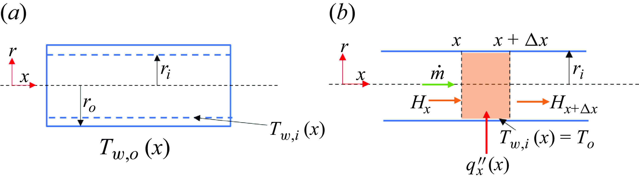


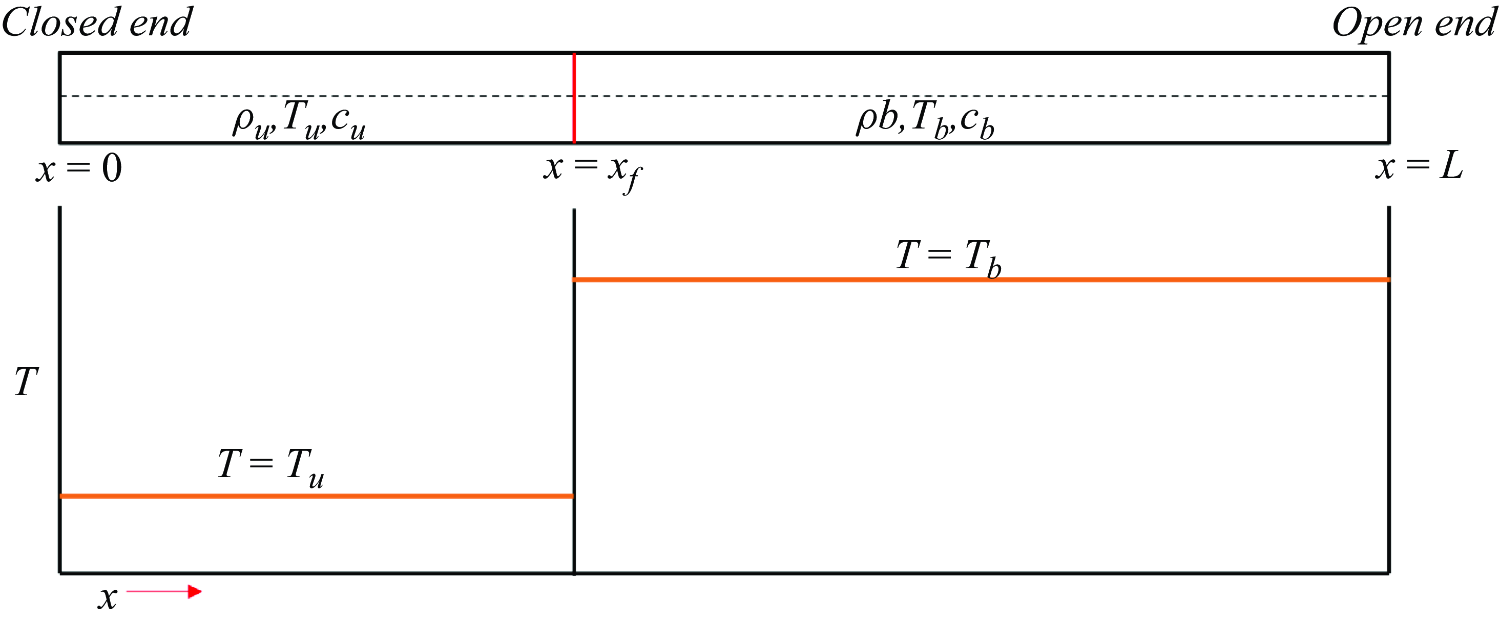


 Open access