


1. Introduction
Injection of  $\textrm {CO}_2$ into underground reservoirs to reduce greenhouse gas emissions, also known as geological carbon sequestration, is one of the major proposed technological solutions to meet future global temperature targets (Bickle Reference Bickle2009; Bui et al. Reference Bui, Adjiman, Bardow, Anthony, Boston, Brown, Fennell, Fuss, Galindo and Hackett2018). During this process, the injected $\textrm {CO}_{2}$ rises as a buoyant plume within the porous aquifer, encountering impermeable cap rocks which force it to spread laterally as a gravity current. As the flow spreads out, capillary forces play a key role in determining the saturation distribution and consequent flow properties via the relative permeability and capillary pressure (Nordbotten & Celia Reference Nordbotten and Celia2011). Heterogeneities in rock properties at the $1 - 100\ \mathrm {cm}$ scales substantially amplify and complicate the effect of variations in pore-scale capillary forces, and are manifest in the large-scale saturation distributions within the $\textrm {CO}_{2}$ current. Hence, in order to ensure safe and efficient sequestration, it is imperative to be able to model how small-scale heterogeneities, which are ubiquitous in all subsurface reservoirs, affect spreading rates at the macroscale (Jackson & Krevor Reference Jackson and Krevor2020; Benham, Bickle & Neufeld Reference Benham, Bickle and Neufeld2021).
The only previous attempts to model such flows in heterogeneous media involve using upscaled relative permeability data, often acquired using numerical calculations or core flooding experiments (Jackson et al. Reference Jackson, Agada, Reynolds and Krevor2018), and applying these to reservoir simulators (Braun, Helmig & Manthey Reference Braun, Helmig and Manthey2005; Cavanagh & Haszeldine Reference Cavanagh and Haszeldine2014; Li & Benson Reference Li and Benson2015; Trevisan, Krishnamurthy & Meckel Reference Trevisan, Krishnamurthy and Meckel2017). However, these studies are often computationally demanding and focus on a specific type of heterogeneity (e.g. over some horizontal/vertical length scale, as investigated by Jackson & Krevor Reference Jackson and Krevor2020). In particular, it is not currently understood how generic small-scale heterogeneities affect the propagation of such large-scale flows. Furthermore, since heterogeneities are usually measured through isolated and sparsely distributed bore hole samples, such measurements often come with a large degree of uncertainty. Yet, despite this, there are very few studies which discuss how such uncertainty at small scales translates to large-scale predictions. Indeed, whilst the studies of Hinton & Woods (Reference Hinton and Woods2020a, Reference Hinton and Woods2020b) investigated how variations in permeability cause shear dispersion for miscible flows, the corresponding effects due to capillary forces within immiscible flows have not yet been addressed. However, as discussed by Jackson & Krevor (Reference Jackson and Krevor2020), these capillary forces associated with the heterogeneities play a critical role during  $\textrm {CO}_{2}$ migration, and, therefore, require careful modelling.
In this study we derive a simple upscaled model for the evolution of an axisymmetric two-phase gravity current beneath an impermeable cap rock, where the structure and distribution of layered heterogeneities is a model input. This simplified approach not only greatly reduces the computational demand of modelling such small-scale details, but also allows us to study a large range of heterogeneities by parameterising them as different types of archetypal sedimentary layering. In this way, we assess how the properties of the heterogeneities affect the macroscale flow, as well as how uncertainty in the measurements is manifest in such flow predictions. Our simple model provides other key insights, such as the self-similar nature of the upscaled gravity current, scaling laws for the speed of propagation and an understanding of where and when the flow transitions between the so-called capillary and viscous limiting behaviours.
In modelling subsurface migration of  $\textrm {CO}_{2}$, a key difficulty is resolving the complex properties of the heterogeneous porous medium. This is a two-fold challenge since resolving all the details of the rock geometry is very computationally intensive, and it is almost impossible to obtain such fine-scaled resolution over field (kilometre) scales from field measurements. Hence, there is a strong motivation for an upscaled modelling approach which describes the bulk, or average effect of heterogeneities on the large-scale flow features. There are many possible levels of upscaling, from the pore scale upwards, as discussed by Krevor et al. (Reference Krevor, Blunt, Benson, Pentland, Reynolds, Al-Menhali and Niu2015). Here we focus on length scales between the size of the heterogeneities and the size of the aquifer. Therefore, in the context of this study small-scale heterogeneities refer to variations on the scale of $10^{-2} - 1\ \mathrm {m}$, and the large-scale flow refers to a gravity current which is typically around $1 - 10\ \mathrm {m}$ thick (Cowton et al. Reference Cowton, Neufeld, White, Bickle, White and Chadwick2016). We do not consider pore-scale heterogeneities, which occur at $10^{-6} - 10^{-3}\ \mathrm {m}$, since these are difficult to resolve with bore hole measurements, and are typically incorporated into bulk properties instead, such as pore entry pressure. Likewise, we do not consider heterogeneities larger than the metre-scale because of the exceedingly long time it would take to establish capillary equilibrium over such length scales.
Heterogeneity types range from variation within the pore structure of a rock to variation in the rock type itself. Owing to the complexity of geological processes, these heterogeneities arise from many different causes, including sedimentary layering, subsequent diagenetic changes in the mineral fabrics and tectonic fracturing and faulting. Each type of heterogeneity affects the flow in a different way, via the action of small-scale capillary forces, thereby presenting a significant challenge for generic upscaling approaches. However, the low computational cost of our approach allows us to investigate a wide variety of heterogeneity types via simple parameterisations of archetypal cases. Among these, we study the effects of lithostatic compaction as well as sedimentary strata with permeability sampled from a probability distribution. The latter case is particularly useful since it captures how the uncertainty in field studies, due to a lack of measurements, is manifest in the uncertainty of modelling predictions.
When upscaling the effect of heterogeneities, a key parameter is the capillary number (Jackson et al. Reference Jackson, Agada, Reynolds and Krevor2018), which is defined as the ratio between horizontal flow-driving pressure gradients (associated with Darcy flow) and vertical capillary pressure gradients (associated with the capillary forces). Hence, in the limit of a small capillary number, known as the capillary limit, the capillary forces due to heterogeneities dominate the flow behaviour, while in the limit of a large capillary number, known as the viscous limit, they have a negligible effect. Many previous studies focus on each of these cases separately, though recently semi-analytical approaches have been derived by Benham et al. (Reference Benham, Bickle and Neufeld2021) and Boon & Benson (Reference Boon and Benson2021) that capture the transition between the viscous and capillary regimes, demonstrating which regions of a confined aquifer are in each of these limits, and which regions are in between the limits. However, gravity was neglected in those studies, restricting the applicability to very thin aquifers.
For  $\textrm {CO}_{2}$ sequestration sites in large aquifers, gravity plays a dominant role in the rise and spreading of the buoyant plume of injected fluid (Nordbotten & Celia Reference Nordbotten and Celia2011). The role of buoyancy is characterised by the ratio between the strength of gravitational forces and capillary forces, and may be quantified by a dimensionless Bond number (Golding, Huppert & Neufeld Reference Golding, Huppert and Neufeld2013) (defined in § 2.3). As discussed by Benham et al. (Reference Benham, Bickle and Neufeld2021), the Bond number is greater than unity for aquifers larger than around ${\sim }1\ \mathrm {m}$ thick, in which case gravity alters the upscaled flow properties significantly. Hence, in this study we focus on the upscaled modelling of such gravity currents, so that more general injection scenarios in larger aquifers can be addressed.
There is a long history of studying gravity currents in porous media, from early work which explored the behaviour in the absence of capillary forces and heterogeneities (Huppert & Woods Reference Huppert and Woods1995), to later studies which investigated the effect of confinement (Pegler, Huppert & Neufeld Reference Pegler, Huppert and Neufeld2014), permeability variations (Hinton & Woods Reference Hinton and Woods2018) and capillary forces (Golding et al. Reference Golding, Huppert and Neufeld2013). Recently, Jackson & Krevor (Reference Jackson and Krevor2020) showed that small-scale capillary heterogeneities can significantly modify the large-scale migration of a buoyant plume within an aquifer. However, their numerical approach is both computationally intensive, and does not provide general scalings for different types of heterogeneity.
The aim of the present study is to quantify the macroscopic effect of a wide range of heterogeneities on the axisymmetric injection of  $\textrm {CO}_{2}$ beneath an impermeable cap rock. The low computational cost of our simple approach allows us to explore different parameterisations of heterogeneities, providing insights into the dominant controls on the evolution of the gravity current. Similar to Benham et al. (Reference Benham, Bickle and Neufeld2021) (though focusing on gravitational effects), we investigate both the viscous limit, the capillary limit and the transition between these limits using a locally defined capillary number that determines where and when heterogeneities play an important role. We show that away from this transition zone the upscaled gravity current is self-similar, where the front moves like the square root of time (like the homogeneous case discussed by Golding et al. Reference Golding, Huppert and Neufeld2013) and the prefactor varies significantly depending on the type and strength of the heterogeneity, as well as the Bond number. In addition, we provide a framework for managing real permeability data with uncertainty in the measurements, illustrating how this uncertainty is manifest in modelling predictions. Finally, we use our upscaled approach to investigate how heterogeneities may have affected the injection of $\textrm {CO}_{2}$ at the Sleipner site in the North Sea (Bickle et al. Reference Bickle, Chadwick, Huppert, Hallworth and Lyle2007).
Our paper is organised as follows. In § 2 we derive a simplified model for the upscaled gravity current, discussing different types of heterogeneities. Section 3 presents both numerical and analytical results, demonstrating that heterogeneities can significantly accelerate plume migration. Moreover, we show that uncertainty due to lack of field measurements has profound consequences on such predictions, especially in post-injection scenarios where capillary effects are enhanced as the plume thins out. In § 4 we apply our results to the case study of the Sleipner project, and finally we close with some concluding remarks in § 5.
2. Upscaled modelling of two-phase gravity currents
In this section we outline the assumptions used to model an upscaled two-phase gravity current in a heterogeneous porous medium, making note of how the saturation of phases varies within the current. Then, we derive the upscaled governing equations and boundary conditions which describe the macroscopic dynamics. Subsequently, we discuss a variety of different types of heterogeneity and how these are manifest in the upscaled properties. Finally, despite the added complexity of the heterogeneities, we demonstrate the self-similar nature of the gravity current, thereby greatly reducing the complexity of the problem.
2.1. Fundamentals of two-phase flow in heterogeneous porous media
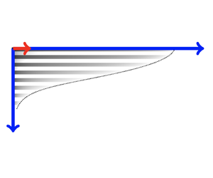
The flow scenario we consider is illustrated in figure 1 with a radial coordinate system  $(r,z)$. A buoyant non-wetting phase (e.g. $\textrm {CO}_{2}$) is injected at a point source at the origin with flow rate $Q$ into a surrounding porous medium saturated with a denser wetting phase (e.g. water). The resulting current spreads out radially under gravity with thickness $z=h(r,t)$ beneath a horizontal impermeable cap rock located at $z=0$. Motivated by the dominant heterogeneity arising from sedimentary layering, we consider a porous medium which has vertically varying permeability $k(z)$ and porosity $\phi (z)$.
Schematic diagram of an axisymmetric gravity current (with constant injection  $Q$) in both the homogeneous case (a) and the heterogeneous case (with sedimentary strata) (c), also illustrating the corresponding vertical non-wetting saturation profiles (b,d), given by (2.10), (2.12) (note the heterogeneity wavelength is exaggerated for illustration purposes). (e) Relationship between mean non-wetting saturation $\bar {s}$ (2.13) and gravity current thickness $h$.
$h$.

We model this scenario using conservation of mass and Darcy's law for two-phase flow (Bear Reference Bear2013). Hence, the governing equations are
 $$\begin{gather} \phi(z) \frac{\partial S_i}{\partial t}+{\boldsymbol{\nabla}}\boldsymbol{\cdot}\boldsymbol{u}_i=0,\quad i=n,w, \end{gather}$$
 $$\begin{gather}\boldsymbol{u}_i={-}\frac{k(z)k_{ri}(S_i)}{\mu_i}{\boldsymbol{\nabla}} \left(\,p_i -\rho_i g \boldsymbol{z} \right),\quad i=n,w, \end{gather}$$
where subscripts  $i=n,w$ indicate non-wetting and wetting phases, and $S_i$, $p_i$, $\boldsymbol {u}_i$, $\rho _i$, $\mu _i$, $k_{ri}(S_i)$ are the saturations, pressures, Darcy velocities, densities, viscosities and relative permeabilities of the two phases. We assume that the pore spaces are filled, such that $S_n+S_w=1$. Furthermore, due to capillary forces, the pressure difference between phases satisfies
 \begin{equation} p_n-p_w=p_c(S_n),\end{equation}
where  $p_c(S_n)$ is the capillary pressure. As is often done, we assume that both $k_{ri}$ and $p_c$ depend on the saturation only for simplicity (though in general they may have more complex dependencies). These are usually approximated with empirical parameterised formulae, such as those proposed by Corey (Reference Corey1954), Brooks & Corey (Reference Brooks and Corey1964) or Chierici (Reference Chierici1984). Here we use the Brooks–Corey and Corey relationships, which are given by
 $$\begin{gather} p_c=p_e(z)(1-s)^{{-}1/\lambda}, \end{gather}$$
 $$\begin{gather}k_{rn}=k_{rn0}s^{\alpha}, \end{gather}$$
where  $p_e(z)$ is the pore entry pressure, $s=S_n/(1-S_{w0})$ is the reduced saturation of the non-wetting phase, $\lambda$ represents the pore size distribution, $k_{rn0}$ is the end-point relative permeability and $\alpha$ is a fitting parameter. The irreducible wetting saturation $S_{w0}$ is the amount of wetting phase that is permanently stored in the pores during drainage flows, and consequently, the end-point relative permeability corresponds to $k_{rn0}=k_{rn}(s=1)$. In this new formulation, the reduced saturation $s$ conveniently varies between 0 and 1.
The pore entry pressure  $p_e(z)$ is the minimum pressure difference required to allow the non-wetting phase to enter the largest pore spaces at a given position. Likewise, as the pressure difference between phases increases, the non-wetting phase is able to enter smaller and smaller pore spaces. Hence, clearly the pore entry pressure depends on the size and geometry of the pores (and, hence, varies vertically), and the same is true for the permeability and porosity. However, whilst this dependence has been measured for specific rock types, it is not fully understood in general. Hence, as is often done, we use power laws to relate these different quantities, such that
 $$\begin{gather} \phi\propto k^{a}, \end{gather}$$
 $$\begin{gather}p_e\propto k^{{-}b}, \end{gather}$$
for some constants  $a, b>0$, which we take to be positive since large pore size corresponds to large porosity, large permeability and small pore entry pressure. As discussed by Cloud (Reference Cloud1941) and Nelson (Reference Nelson1994), we do not expect these constants to be the same for different rock types. Therefore, we keep them in general form for this analysis. However, we note a commonly used scaling proposed by Leverett (Reference Leverett1941), $p_e\sim (\phi /k)^{1/2}$ which implies $b=1/2(1-a)$.
Motivated by field observations of gravity currents (e.g. see Cowton et al. (Reference Cowton, Neufeld, White, Bickle, White and Chadwick2016), where the aspect ratio of the gravity current at Sleipner was calculated to be less than  ${\sim }1/1000$) and following Golding et al. (Reference Golding, Neufeld, Hesse and Huppert2011, Reference Golding, Huppert and Neufeld2013), we assume that the gravity current is long and thin, such that the vertical velocity is much smaller than the horizontal velocity $w_i\ll u_i$. In this case, the pressure within each phase is approximately hydrostatic,
 \begin{equation} \frac{\partial p_i}{\partial z}=\rho_i g,\quad i=n,w,\end{equation}
and consequently, (2.8) is integrated to match the capillary pressure (2.3), giving
 \begin{equation} p_c={-}\Delta \rho g (z-h) + p_0,\end{equation}
where  $p_0$ is the capillary pressure at the edge of the gravity current $(z=h)$ and $\Delta \rho =\rho _w-\rho _n$. The saturation is calculated by combining (2.4) and (2.9), enforcing the physical lower bound on $s$, such that
 \begin{equation} s=\max \left\{ 1-\left[\frac{p_0}{p_e(z)}+\frac{\Delta \rho g (h-z)}{p_e(z)}\right]^{-\lambda},\ 0 \right\}.\end{equation}
To determine the value of  $p_0$ we consider that the edge of the gravity current is defined as the boundary below which no saturation of non-wetting phase exists. Hence, from (2.9), (2.10), it is sufficient to ensure that $s=0$ for all $z>h$ if we choose $p_0=\min p_e(z)$. In other words, by setting the capillary pressure at the edge of the gravity current as the smallest required pressure difference to invade any pores in the aquifer, we guarantee that anywhere below the edge of the gravity current $(p_c< p_0)$ no saturation will be found. Therefore, even though there may be disconnected regions of non-wetting phase within $0\leqslant z\leqslant h$ (e.g. see figure 1c,d), there will never be such regions for $z>h$.
The saturation distribution (2.10) represents a balance between capillary forces (due to heterogeneities) and gravitational forces. However, this is only valid for situations where capillary forces are large enough to drive the saturation into regions of larger pore space, or equivalently, when the capillary number is small. Therefore, in general, the saturation distribution must depend on the local capillary number  $N_c$, which is given as the ratio between the horizontal flow-driving pressure gradient and the typical vertical gradient in pore entry pressure (Benham et al. Reference Benham, Bickle and Neufeld2021). For the former, we use the pressure gradient of the non-wetting phase ${\partial p_n}/{\partial r}$, and for the latter we use ${\Delta p_e}/{h}$, where $\Delta p_e=\max p_e(z) - \min p_e(z)$ is the maximum difference in pore entry pressure across the aquifer (constant), and the gravity current thickness $h$ is used as the vertical length scale. Hence, the capillary number is given by
 \begin{equation} {N}_c=\left|\frac{h}{\Delta p_e}\frac{\partial p_n}{\partial r}\right|.\end{equation}
In the limit of very small capillary number  $N_c\ll 1$, also known as the capillary limit, the saturation distribution (2.10) remains accurate. However, when the capillary number is very large, also known as the viscous limit, capillary forces due to heterogeneities are effectively negligible (i.e. we can ignore pore entry pressure variations $p_e(z)=p_0$), and the saturation distribution becomes
 \begin{equation} s= 1-\left[ 1+\frac{\Delta \rho g (h-z)}{p_0}\right]^{-\lambda} ,\end{equation}
which is identical to the homogeneous case addressed by Golding et al. (Reference Golding, Huppert and Neufeld2013).
For an intermediate capillary number (i.e. when the flow is neither in the viscous limit nor the capillary limit), the saturation distribution lies in between (2.10) and (2.12), and, therefore, the expression for the saturation must contain the capillary number itself  $s=s(z,h,{N}_c)$. Typically, the dependence of the saturation on the capillary number is logarithmic (Virnovsky, Friis & Lohne Reference Virnovsky, Friis and Lohne2004; Benham et al. Reference Benham, Bickle and Neufeld2021), as with the upscaled flow properties, and we will return to address this later in § 3.3.
In figure 1(c) we illustrate a radially symmetric gravity current in a heterogeneous layered medium composed of sedimentary strata. We contrast this to the classic homogeneous case in figure 1(a) (as studied by Golding et al. Reference Golding, Huppert and Neufeld2013), which is equivalent to the upscaled viscous limit ( $N_c\gg 1$) for a heterogeneous medium. (We note that although the upscaled description of the viscous limit is mathematically identical to the homogeneous case, the model would still have to account for flow variations due to permeability gradients through an effective permeability. The saturation would, however, be identical to the homogeneous case.) For each case, we plot typical vertical saturation profiles in figure 1(b,d). In the homogeneous case the saturation distribution satisfies a balance between capillary and buoyancy forces, so that lighter regions (of high saturation) are pushed towards the cap rock. In the heterogeneous case the same overall balance is sustained, but within that balance capillary forces push the saturation into layers where the pores are larger. Hence, significant oscillatory behaviour is observed within the vertical saturation profile, including patches where the saturation drops to zero. This corresponds with regions where the pore spaces are too small to allow any non-wetting phase (i.e. the zero value is chosen in (2.10)). Hence, one interesting consequence of heterogeneities is that they modify the mean saturation value in the gravity current. In figure 1(e) we plot the mean saturation, defined as
 \begin{equation} \bar{s}(h)=\frac{1}{h}\int_0^{h} s\,\mathrm{d}z,\end{equation}
whilst varying the gravity current thickness  $h$ for both the homogeneous and heterogeneous cases. In both cases $\bar {s}$ is an increasing function of $h$, but the heterogeneous case always has a lower mean value. This is due to the substantial fraction of the gravity current with zero saturation.
2.2. Upscaled model: governing equation and boundary conditions
Having discussed the flow scenario and laid down the key assumptions, now we outline the upscaling procedure, deriving a single governing equation and accompanying boundary conditions for the macroscopic description of the gravity current.
To do so, (2.8) is integrated to obtain the pressure, and then the conservation of mass equation for the non-wetting phase (2.1) is integrated between  $z=0$ and $z=h(r,t)$, such that
 \begin{equation} \varphi\frac{\partial}{\partial t} \int_0^{h} \hat{\phi}(z) s \,\mathrm{d}z -\frac{u_b}{r}\frac{\partial}{\partial r}\left[ \frac{r}{k_0k_{rn0}}\frac{\partial h}{\partial r} \int_0^{h} k(z) k_{rn}(s) \,\mathrm{d}z \right]=0, \end{equation}
where  $\varphi =(1-S_{w0})\phi _0$ is the reduced porosity scaling, $\phi _0$ and $k_0$ are typical scalings for the porosity and permeability (where $\hat {\phi }=\phi /\phi _0$), and $u_b={k_0k_{rn0} \Delta \rho g}/{\mu _n}$ is the buoyancy velocity.
We note that the flow of the wetting phase is ignored in this analysis under the long-thin approximation. Essentially, the flow of the non-wetting phase within the gravity current decouples from the flow of the wetting phase, which is not present at leading order. Nevertheless, multiphase effects are still manifest at leading order via the multiphase properties, such as the relative permeability and capillary pressure. However, as we discuss later in § 2.3, this assumption breaks down if the contrast in permeabilities of the layers becomes very large. In particular, if there are regions of very low permeability, these will act as a vertical obstruction to the flow. In such situations, as discussed by Pegler et al. (Reference Pegler, Huppert and Neufeld2014), the flow must be treated as confined, where the displacement of the ambient fluid and the viscosity contrast between phases alter the dynamics and, therefore, can no longer be ignored. We give more details of this consideration in the next section.
We also note that (2.14) is already an upscaled description of the flow, since the heterogeneities are only manifest within the integrals. Hence, (2.14) represents how the heterogeneities affect the evolution of the gravity current in a spatially averaged sense. Such an upscaling approach is desirable, since we wish to avoid having to resolve all the heterogeneities, both to reduce computation time, and also because the low resolution of field measurements means that such details are uncertain anyway.
It is convenient to write (2.14) in a more standard diffusion equation form to render it amenable to conventional analysis. Therefore, by switching variables to the integrated saturation  $\mathcal {S}(h,{N}_c)$, which is defined as
 \begin{equation} \mathcal{S}=\varphi\int_0^{h} \hat{\phi}(z) s\,\mathrm{d}z, \end{equation}
(2.14) may be rewritten as
 \begin{equation} \frac{\partial \mathcal{S}}{\partial t} =\frac{1}{r}\frac{\partial}{\partial r}\left[ r \mathcal{F}(\mathcal{S},{N}_c) \frac{\partial \mathcal{S}}{\partial r} \right],\end{equation}
where the flux is given by
 \begin{equation} \mathcal{F}=\frac{u_b}{k_0k_{rn0}}\left[\frac{\mathcal{K}(h,{N}_c)}{\mathcal{S}_h(h,{N}_c)}\right],\end{equation}
and the two functions  $\mathcal {K}(h,{N}_c)$ and $\mathcal {S}_h(h,{N}_c)$ are defined as
 $$\begin{gather} \mathcal{K}=\int_0^{h} k(z) k_{rn}(s)\,\mathrm{d}z, \end{gather}$$
 $$\begin{gather}\mathcal{S}_h=\varphi\int_0^{h} \hat{\phi}(z) {\partial s}/{\partial h}\,\mathrm{d}z= \frac{\partial\mathcal{S}}{\partial h}. \end{gather}$$
Further details of this coordinate transformation are presented in Appendix B. We note that  $\mathcal {S}$ has dimensions of length, and $\mathcal {F}$ has dimensions of length squared over time. Therefore, (2.16) is just a standard diffusion equation for the total volume of the non-wetting phase (per unit area), where the flux is a nonlinear function that represents how capillary forces modify the flow. Hence, there is an interesting analogy between our scenario and a viscous gravity current, where the flux function represents how viscous forces modify the flow (e.g. plug flow, Poiseuille flow, etc…). As we will find out later, $\mathcal {F}$ is sometimes well approximated by a power law of $\mathcal {S}$, and the solutions to such equations are detailed by a large, historical body of literature (see Huppert (Reference Huppert1982) for example).
In general, (2.16) must be solved in tandem with the equation for the capillary number (2.11). Therefore, writing (2.11) in terms of the integrated saturation  $\mathcal {S}$, we arrive at the transcendental equation for the capillary number,
 \begin{equation} {N}_c=\frac{\Delta\rho g}{\Delta p_e}\left|\frac{h(\mathcal{S},{N}_c)}{\mathcal{S}_h(h(\mathcal{S},{N}_c),{N}_c)}\frac{\partial \mathcal{S}}{\partial r}\right|,\end{equation}
where  $h$ is written in terms of $\mathcal {S}$ under the assumption that (2.15) has a uniquely defined inverse (which we later find to be the case).
For the remainder of this study (up until § 3.3), we restrict our attention to the two limiting cases of small and large capillary number (capillary and viscous limits), where the saturation is given by (2.10) or (2.12) and the flux is just given by  $\mathcal {F}=\mathcal {F}(\mathcal {S})$, thereby decoupling (2.16) and (2.20). However, later in § 3.3 we address the case of an intermediate capillary number, for which the equations must be solved in tandem.
The governing equation (2.16) must be accompanied by some initial and boundary conditions to create a well-posed system. Firstly, we define the nose of the gravity current at position  $r=r_N(t)$, at which the thickness is zero, such that
 \begin{equation} \left.\mathcal{S}\right|_{r=r_N(t)}=0.\end{equation}
Secondly, we impose zero flux through the nose of the current,
 \begin{equation} 2{\rm \pi} \left[r\mathcal{F}\frac{\partial \mathcal{S}}{\partial r}\right]_{r=r_N(t)}=0.\end{equation}
Finally, following Golding et al. (Reference Golding, Huppert and Neufeld2013), we impose global conservation of mass of the non-wetting phase, such that
 \begin{equation} 2{\rm \pi}\int_0^{r_N(t)} r\mathcal{S}\,\mathrm{d}r=Qt,\end{equation}
or equivalently, we impose the input flux at the origin,
 \begin{equation} -2{\rm \pi} \left[r\mathcal{F}\frac{\partial \mathcal{S}}{\partial r}\right]_{r=0}=Q.\end{equation}
The finite flux value  $Q$ in (2.24) indicates that the gradient ${\partial \mathcal {S}}/{\partial r}$ must become infinite as $r\rightarrow 0$. Therefore, it is expected that the long-thin approximation made earlier may become invalid very close to injection. Furthermore, near the nose of the gravity current $r=r_N$, where the gravity current becomes thinner than the heterogeneity length scale, we do not expect our upscaled approximation to be accurate.
2.3. Incorporating heterogeneity
To close the system, we must choose a type of vertical heterogeneity. Since we have used power laws  $a,b$ to relate the porosity and pore entry pressure to the permeability, we need only choose a functional form for $k(z)$. Whilst in general this function may vary in three dimensions (i.e. $k(\boldsymbol {x})$), here we restrict our attention to pure vertical variation since, not only does this capture the leading-order behaviour for sedimentary layering, but also because this is consistent with the long-thin approximation of a gravity current made earlier.
To model the permeability, we have a variety of different physically motivated choices which we list in table 1 and plot in figure 2. Firstly, sedimentary strata represent a periodic deposition of two different types of sediments, such that the permeability alternates between two values,  $k_{low}$ and $k_{high}$, in a periodic array of layers, where the width ratio of each of these is given by $H_{low}/H_{high}$ (see figure 2a–c). Unlike the sedimentary strata, which are uniformly deposited in each layer, turbidites represent the deposition of sediments from the continuous arrival of turbidity currents, such that within each layer the permeability varies linearly. The sign of the linear slope indicates that layers become more permeable as one descends deeper, since this corresponds to the early/late arrival of large/small particles in a turbidity current. Thirdly, we consider a permeability profile which is generated by randomly sampling from a distribution, or spectrum, of permeability values, spread out logarithmically. This case is motivated by realistic measurements of sedimentary strata which are often noisy and aperiodic. Finally, we consider a compacted rock, where the permeability decreases with depth due to the buildup of lithostatic pressure over time.
Illustrations of the different types of heterogeneity we consider, where the heterogeneity is characterised by variation of the permeability with depth. Plots (a–f) represent the deposition of sediments through various geological mechanisms, whereas (g) represents compaction due to lithostatic pressure. In (a–c) we illustrate the case of sedimentary strata with greyscale permeability maps for three different values of the width ratio between low/high permeability regions  $(H_{low}/H_{high})$. In the spectrum case (f) we display the probability density function (p.d.f.) of the permeability which is randomly sampled from a uniform distribution on a logarithmic scale.

Definitions of the different types of heterogeneity (characterised by the permeability), as displayed in figure 2. Sedimentary strata take binary permeability values  $k_{low},k_{high}$, with the width ratio of low/high regions given by $H_{low}/H_{high}$. Turbidites, the deposits of turbidity currents, consist of a periodic array of layers with linearly varying permeability, where the wavenumber $n$ is considered in the limit $nh\rightarrow \infty$. In the spectrum case, permeability is a series of strata, where each layer has permeability taken from a uniform random distribution, distributed logarithmically across range $[k_{low}, k_{high}]$. Likewise, the widths of the layers are taken from a uniform random distribution on a linear scale. Compacted rock corresponds to a permeability profile which decreases with depth under a power law $\beta$, starting with a finite value at $z=0$.

Although there are many other possible choices for the permeability, we restrict our investigation to these four examples since they are canonical cases from which we may learn about the fundamental effects of heterogeneities. Each case is parameterised, either by the ratio of the permeabilities and widths of the lowest–highest permeability regions  $k_{low}/k_{high}$, $H_{low}/H_{high}$, or by the compaction power law $\beta$, which represents the strength of the compaction effect.
It is important to note the possible limitations on these parameters. In particular, sufficiently low permeability layers may cause a vertical obstruction, such that an unconfined description of the gravity current is no longer applicable. To investigate the limitations on the permeability ratio  $k_{low}/k_{high}$, we have performed a set of numerical simulations of the two-dimensional miscible Darcy equations using the DarcyLite finite element package in Matlab, adapted to account for gravity (Liu, Sadre-Marandi & Wang Reference Liu, Sadre-Marandi and Wang2016; Harper et al. Reference Harper, Liu, Tavener and Wildey2021). The miscible Darcy equations are equivalent to the immiscible equations (2.1)–(2.2) in the limit where the relative permeabilities become independent of the phases, $k_{rn},k_{rw}\rightarrow 1$, and the phase pressures equalise such that $p_c\rightarrow 0$. Studying the miscible flow problem allows us to investigate the applicability of upscaling for small values of the permeability ratio $k_{low}/k_{high}$ (i.e. large permeability contrasts) without accounting for the more complex effects of immiscible phase saturations. We do not display the numerical results here, since a rigorous analysis of this query is outside the scope of this paper, but we describe our findings in writing instead.
For very small values of the permeability ratio (e.g.  $k_{low}/k_{high}=0.001$), there are several important observations from these numerical simulations. At early times, due to the effective obstruction from the low permeability layers, the injection is focused within the nearest high permeability layers instead, and behaves approximately like a confined flow in which the pressure has significant streamwise gradients (i.e. deviating away from the hydrostatic condition (2.8)). As a result, the shape of the gravity current is highly distorted and loses its self-similar structure. At later times, once the gravity current has invaded a sufficient number of vertical layers, it begins to assume self-similar dynamics and the pressure becomes hydrostatic to good approximation. Therefore, there is no strict lower bound on the permeability ratio $k_{low}/k_{high}$ for an upscaling procedure, but rather this becomes a question of temporal and spatial scales. In other words, for any non-zero permeability ratio, given enough time and spatial extent, such an injection will eventually resemble a self-similar gravity current and is therefore amenable to upscaling. However, to avoid dealing with the prolonged transient effects that precede self-similarity in the case of very small permeability ratios, for the remainder of this study, we restrict our attention to $k_{low}/k_{high}\geqslant 0.01$.
Continuing our upscaling analysis we note that, given a particular type of heterogeneity  $k(z)$ and power laws $a,b$ for the porosity and pore entry pressure, the integrals (2.15), (2.18)–(2.19) must first be calculated before we can solve (2.16). For general values of $a,b$, these integrals must be calculated numerically, using a trapezoidal integration rule for example (see code in the supplemental material). In the layered cases, we wish to remove the dependence of these integrals on the heterogeneity wavelength, since it is undesirable to have upscaled properties like $\mathcal {F}$ that oscillate depending on the gravity current thickness. Therefore, instead of resolving all of the details of the flow, we build a macroscopic picture of the gravity current. This is similar to the approach of Boon & Benson (Reference Boon and Benson2021) who calculated the bulk flow speeds for an upscaled Buckley–Leverett problem in layered media, but contrasts the upscaling studies of Anderson, McLaughlin & Miller (Reference Anderson, McLaughlin and Miller2003) (for a single-phase gravity current) and Jackson & Krevor (Reference Jackson and Krevor2020) (for a two-phase gravity current), where some of the small-scale flow details due to heterogeneities are resolved.
In the case of sedimentary strata, since  $k$ (and, therefore, $p_e$ and $\phi$) takes either one of two possible values, integrals can be simply decomposed into bulk fractions,
 \begin{equation} \int\,\cdot\,\mathrm{dz}=\frac{H_{low}\displaystyle\int_{k_{low}}\,\cdot\,\mathrm{d}z+H_{high}\int_{k_{high}}\,\cdot\,\mathrm{d}z}{ H_{low}+H_{high}},\end{equation}
thereby removing the need to resolve individual layers. A similar approach can be taken in the case of the permeability spectrum, although in that case (2.25) is replaced by a sum over the number permeability values sampled from the random distribution. (Note that in the case of the permeability spectrum, we sample  $N$ pairs of values $\{k_i,H_i\}$ ( $i=1,\ldots ,N$) from a random distribution of permeabilities and layer widths. Once sampled, it does not matter how these values are arranged. Therefore, a bulk decomposition like (2.25) is still possible.) However, in the case of the turbidites, to remove the dependence on the wavenumber $n$ (as defined in table 1), the integrals must be calculated with a fine numerical scheme for a large but finite value of $nh\gg 1$.
The most salient features of this analysis are the integrated saturation  $\mathcal {S}(h)$ and the flux $\mathcal {F}({h})$, since $\mathcal {F}$ allows us to solve the diffusion equation (2.16), and $\mathcal {S}$ allows us to calculate the gravity current thickness by way of inversion. These both depend on a number of non-dimensional parameters. Ignoring the capillary number (since for now we restrict our attention to $N_c\ll 1$ or $N_c\gg 1$) there are a total of eight non-dimensional parameters which govern the problem. These consist of the heterogeneity parameters $k_{low}/k_{high}$, $H_{low}/H_{high}$, $\beta$ (if compaction present); the power laws relating porosity and pore entry pressure to the permeability $a$,
$a$,  $b$; the Brooks–Corey parameters $\lambda$, $\alpha$; and finally the Bond number, which is defined as
 \begin{equation} {Bo}=\left( \frac{Q \Delta \rho g \mu_n}{k_0 k_{rn0} p_{0}^{2}}\right)^{1/2}.\end{equation}
The Bond number, which can alternatively be written as  $Bo={\Delta \rho g H}/{p_0}$, where $H=\sqrt {Q/u_b}$ is the buoyancy length scale, is interpreted as the ratio between buoyancy forces and capillary forces. We note that for situations in which the injection flux is switched off (e.g. in post-injection scenarios), the Bond number must be redefined in terms of the thickness of the current, which evolves according to a fixed volume constraint, as we discuss in the conclusion.
The Bond number (2.26) largely controls the saturation distribution (2.10), (2.12), which is evident upon dimensional analysis. For example, when  $Bo\gg 1$, the saturation, written in dimensionless form, approximates to
 \begin{equation} s= 1-\left[\frac{1}{{p}_e({z})/{p}_0}+\frac{{Bo} ({h}/H-{z}/H)}{{p}_e({z})/p_0}\right]^{-\lambda}\approx 1.\end{equation}
It should be noted that the above expression is not valid for extreme pore entry pressure variations ( $p_e/p_0\gg 1$), and in such cases the criterion for uniform saturation ( $s\approx 1$) must be replaced by $Bo\times p_0/p_e\gg 1$. However, all of the cases we consider in this study have moderate power laws (2.7), resulting in first-order pore entry pressure variations $p_e/p_0=\mathcal {O}(1)$.
We note that some of the above parameters have already been studied by other authors. For example, the power laws  $a,b$ were already addressed by Benham et al. (Reference Benham, Bickle and Neufeld2021) and the Brooks–Corey parameter $\lambda$ was studied by Golding et al. (Reference Golding, Huppert and Neufeld2013). In particular, variations in saturation are amplified by larger values of $a$ (i.e. stronger pore entry pressure heterogeneity $p_e(z)$) or smaller values of $\lambda$ (i.e. wider distribution of pore space). Meanwhile, larger values of $b$ (i.e. stronger permeability heterogeneity $k(z)$) make the flux more nonlinear via (2.18). Hence, the effects of heterogeneities are amplified with larger values of $a$ or $b$, and smaller values of $\lambda$.
For the remainder of the current study, we focus on the heterogeneity parameters  $k_{low}/k_{high}$, $H_{low}/H_{high}$, $\beta$ and the Bond number as the key parameters of interest. We use the homogeneous case $k_{low}/k_{high}=1$ as a proxy to study the viscous limit behaviour $N_c\gg 1$, since they are equivalent (see bracketed comment in § 2.1). We fix the remaining parameters at typical values $a=1/7$, $b=3/7$, $\lambda =3$ and $\alpha =4$, which we have extracted from a variety of different sources (Leverett Reference Leverett1941; Golding et al. Reference Golding, Neufeld, Hesse and Huppert2011; Berg, Oedai & Ott Reference Berg, Oedai and Ott2013; Bickle et al. Reference Bickle, Kampman, Chapman, Ballentine, Dubacq, Galy, Sirikitputtisak, Warr, Wigley and Zhou2017). Up until § 4 we keep the same values for these parameters so that we can focus on the effect of the heterogeneities instead, but we note that our approach is by no means restricted to these values.
Nevertheless, continuing with these parameter values, we illustrate how the flux  $\mathcal {F}$ depends on the type of heterogeneity and the Bond number in figure 3(a–c). For each of the layered cases, we use a permeability ratio value of $k_{low}/k_{high}=0.1$, whereas in the compacted case we use a power law of $\beta =1$. In all cases (except the spectrum case) the flux is well approximated by a power law $\mathcal {F}\propto \mathcal {S}^{\psi }$ for some value of $\psi$ between $1/2$ and $2$. In some cases, as we will show later in § 3.2, these power laws can be derived analytically.
(a–c) Variation of the flux  $\mathcal {F}$ (2.17) of the integrated saturation $\mathcal {S}$ in (2.16) for different values of the Bond number Bo. Both $\mathcal {F}$ and $\mathcal {S}$ are normalised by reference values (measured at twice the mid-range value of the gravity current thickness, $h_{half}=h(r_N(t)/2,t)$) for illustration purposes. In each plot we indicate power law values of $1/2$, $1$ and $2$ with dotted lines for comparison. (d) Analogy between a two-phase gravity current in a heterogeneous porous medium and a non-Newtonian viscous gravity current with viscosity power law $\mu \propto (\partial u/\partial z)^{\kappa }$. The resultant flux power law is given by $\int _0^{h} u\,\mathrm {d}z\propto h^{2+1/(1+\kappa )}$, as indicated with the blue curve. Red dashed lines illustrate particular power law values of interest.

Figure 11 in Appendix A displays the integrated saturation  $\mathcal {S}$, as well as the velocity distribution $u_n\propto \Delta \rho g k(z)k_{rn}(s)/\mu _n$ within the gravity current. There are several interesting observations to make. Firstly, no matter which type of heterogeneity nor which Bond number we choose, the integrated saturation $\mathcal {S}(h)$ is always a monotonically increasing function, such that the inversion $h=\mathcal {S}^{-1}(\mathcal {S})$ is always well posed. Secondly, we note that there is an interesting interpretation to the value of the flux power law $\psi$, by way of analogy to viscous gravity currents. In the governing diffusion equation for a classic viscous gravity current, the flux power law relates to the velocity distribution within that current. For example, the velocity distribution for Poiseuille flow, which varies quadratically in the vertical coordinate, when integrated gives a cubic flux power law. Likewise, a uniform plug flow, when integrated gives a linear flux power law.
In general, any viscous gravity current flux power law can be achieved by considering a shear thinning/thickening power law viscosity  $\mu \propto (\partial u/\partial z)^{\kappa }$. Then, the lubrication balance $\partial /\partial z[\mu \partial u/\partial z] \sim \partial p/\partial x$ can be integrated to give a flux $F=\int _0^{h} u\,\mathrm {d}z$ which obeys the power law $F\propto h^{2+1/(1+\kappa )}$. This is illustrated in figure 3(d), indicating specific cases with dashed lines. For example, a shear thinning fluid with power law $\kappa =-5/3$ will produce a flux with power law $F\propto h^{1/2}$. Whilst our upscaling problem is very different from a non-Newtonian viscous gravity current, the analogy is nevertheless useful in helping to relate the flux functions observed in figure 3(a–c), to the velocity distributions within our gravity current (which are displayed in figure 11(b,d,f) in Appendix A).
Now that all the steps in our approach have been outlined, we summarise our methodology for analysing the gravity current in figure 4. This illustrates the steps between initially choosing a heterogeneity type and finally solving for the gravity current thickness  $h$. We have provided some example codes in the supplemental materials to demonstrate these steps in the case of sedimentary strata, including how to numerically calculate the flux functions.
Schematic illustration of our methodology, with stages going from left to right (a–e). We start by parameterising the heterogeneity  $k(z),p_e(z),\phi (z)$; then we use (2.10) to determine the saturation distribution $s(z,h)$; then we obtain the velocity distribution $u_n\propto \Delta \rho g k(z)k_{rn}(s)/\mu _n$ (velocities for high and low permeability regions are illustrated in addition to the mean); then from this we calculate the integrals comprising the flux $\mathcal {F}(h(\mathcal {S}))$ (2.17); then finally we use (2.16) to calculate the gravity current thickness $h$ (via $\mathcal {S}(h)$).

2.4. Discussion of self-similarity and the numerical scheme
There is a final simplification that can be made owing to a coordinate invariance, which allows calculation of the solution using a simple numerical scheme. In particular, much like the classic single-phase axisymmetric gravity current discussed by Lyle et al. (Reference Lyle, Huppert, Hallworth, Bickle and Chadwick2005), the heterogeneous case is self-similar. (Note that the two-dimensional case is not necessarily self-similar. The two-dimensional gravity current thickness scales like  $h\sim t^{1/3}$, such that the flux function $F(h)$ cannot be written in a general self-similar form. However, this becomes possible in certain specific cases (e.g. a linear power law $F\propto h$, as discussed by Huppert & Woods Reference Huppert and Woods1995).) Upon inspection, for constant flux, our governing equation (2.16) (under the assumption of viscous $N_c\gg 1$ or capillary $N_c\ll 1$ limits) admits the similarity variables
 $$\begin{gather} \eta=(\varphi^{2}/Q u_b)^{1/4} r t^{{-}1/2}, \end{gather}$$
 $$\begin{gather}\mathcal{S}={H}{\varphi}f(\eta), \end{gather}$$
where the nose of the gravity current is located at  $\eta =\eta _N$ for some constant $\eta _N$ which we will determine shortly. To further simplify the equations, and to convert to a unit interval domain, we write our system in terms of the variables $y=\eta /\eta _N$ and $\hat {f}(y)=f(\eta )$. In this way, the governing equation for the integrated saturation (2.16) and the boundary conditions (2.21)–(2.23) become
 $$\begin{gather} \left[y \hat{\mathcal{F}}(\,\hat{f}) \hat{f}'\right]'+\tfrac{1}{2}\eta_N^{2} y^{2} \hat{f}'=0, \end{gather}$$
 $$\begin{gather}\hat{f}(1)=0, \end{gather}$$
 $$\begin{gather}\hat{\mathcal{F}}(\,\hat{f}(1)) \hat{f}'(1)=0, \end{gather}$$
 $$\begin{gather}\eta_N^{2}\left[2{\rm \pi}\int_0^{1} y\hat{f}(y)\,\mathrm{d} y\right]=1, \end{gather}$$
where  $\hat {\mathcal {F}}=\mathcal {F}\varphi /u_bH$. The system can be solved numerically using a simple finite difference scheme, starting at $y=1$ and marching back towards $y=0$. To find the constant $\eta _N$, we start with an initial guess $\eta _{N_0}$, and then use Newton's method to iteratively solve the flux condition (2.33) (see the code in the supplemental material available at https://doi.org/10.1017/jfm.2021.523).
We make the key observation that, independent of the form of  $\hat {\mathcal {F}}(\,\hat {f})$, the gravity current is self-similar, with a nose that moves like the square root of time. Hence, the heterogeneities are only capable of modifying the prefactor $\eta _N$ for the nose speed, not the power law (which is always $r\sim t^{1/2}$). However, the heterogeneities may also change the shape of the gravity current via $\mathcal {F}$ and $\mathcal {S}$.
As discussed later in § 3.3, in the case where the capillary number is neither small nor large, the flux must depend on the capillary number itself. In this case, since the capillary number involves derivatives of  $\mathcal {S}$ with respect to $r$, this modifies the form of the governing equation (2.16), rendering such similarity variables inadmissible. Over time the solution changes from a viscous limit regime (self-similar) to a capillary limit regime (self-similar), but the transition itself, therefore, cannot be self-similar.
3. Results: viscous limit, capillary limit and transition
Our results comprise the following three different cases.
(i) The capillary number is large throughout the aquifer (viscous limit), in which case the upscaled problem is equivalent to the homogeneous case.
(ii) The capillary number is small throughout the aquifer (capillary limit), in which case the upscaled problem is dominated by the effect of the heterogeneities.
(iii) The capillary number varies across the aquifer, such that different regions simultaneously lie within the viscous limit and the capillary limit, and other regions lie between these limits.
We start by addressing the former two cases (viscous and capillary limits), for which the problem is self-similar. The homogeneous case is used to study the viscous limit (since they are equivalent in an upscaled sense) and the heterogeneous cases are used to study the capillary limit. The gravity current thickness must be calculated numerically by solving the ordinary differential equation (ODE) system (2.30)–(2.33). In specific limiting cases, such as when the Bond number is very large or very small, analytical progress can be made. We first present our numerical results which we use to understand the broad effect of the heterogeneities across large parameter regimes. Then, we use asymptotic analysis to help interpret the results in certain limiting cases. Finally, we address the transition between the viscous and capillary limits, for which the full partial differential equation (PDE) system (2.16), (2.21)–(2.23) must be solved in tandem with an algebraic equation for the local capillary number (2.20).
3.1. Numerical solution in the viscous and capillary limits
The capillary limit numerical solution for different types of heterogeneity is plotted in figures 5 and 6 for Bond number values between  $Bo =10^{-2}$ and $Bo =10^{2}$. Typical saturation profiles are also displayed as inserts in each plot. To compare the different profiles, we have normalised the thickness by twice its mid-range value $h_{half}=h(r_N(t)/2,t)$. The radial coordinate is normalised by the nose position $r_N(t)$ so that the shape remains on a fixed domain for all time. For now, we do not include plots of the viscous limit numerical solutions, since these are very similar to the study by Golding et al. (Reference Golding, Huppert and Neufeld2013). However, shortly we will use these as a reference when comparing the different types of heterogeneities.
Numerical results for the capillary limit in the case of sedimentary strata (a,c,e) and turbidites (b,d,f) (with  $k_{low}/k_{high}=1/3,H_{low}/H_{high}=1$). From top to bottom, capillary forces become less important with respect to gravitational forces. The radius $r$ is given in terms of the nose position $r_N(t)$, and the thickness $h$ is normalised by the reference value $2h_{half}=2h(r_N(t)/2,t)$ for the sake of comparison. The heterogeneity wavelength is exaggerated for illustration purposes. In each plot inserts illustrate the vertical saturation profile, normalised by the uppermost value $s_0=s(0)$.
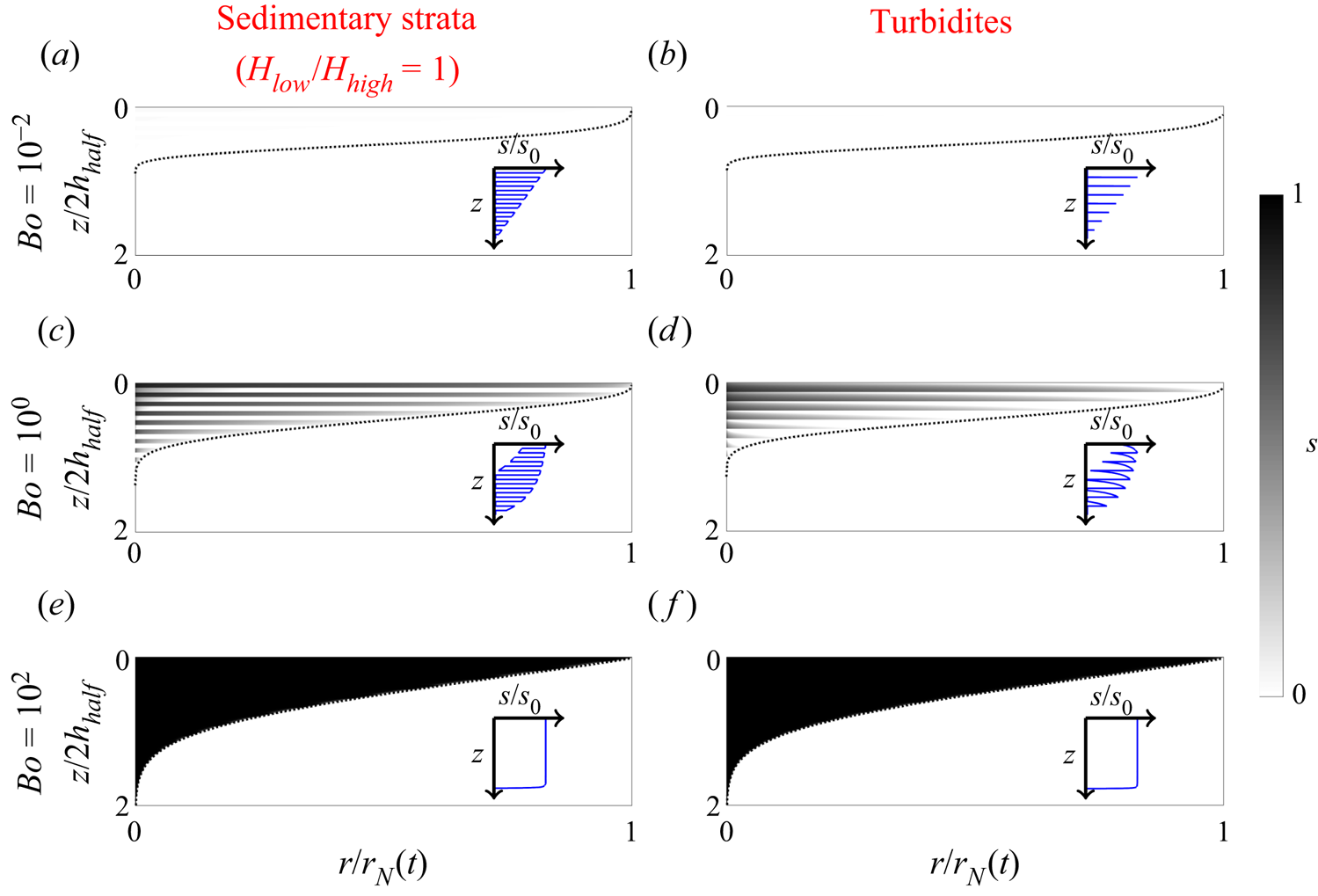
Numerical results for the capillary limit in the case of spectrum permeability (a,c,e) (with mean permeability ratio  $k_{low}/k_{high}=0.04$) and compacted rock (b,d,f) (with compaction power law $\beta =1$). In each plot inserts illustrate the vertical saturation profile, normalised by the uppermost value $s_0=s(0)$. The heterogeneity wavelength is exaggerated for illustration purposes.
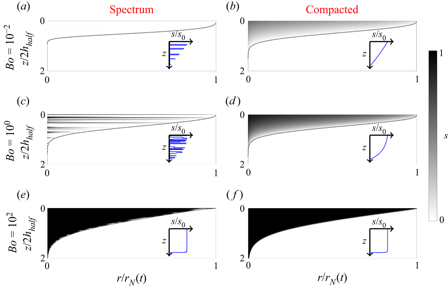
Let us first focus on the non-compacted cases in the capillary limit (figures 5 and 6a,c,e). For a small Bond number  $Bo\ll 1$, the saturation becomes near zero $s\approx 0$, but with spikes of linearly increasing magnitude that represent the thin regions where the permeability is near its maximum value $k\approx k_{high}$. As we increase the Bond number towards unity, the saturation becomes larger, with an overall curved profile and significant oscillations. At high Bond number, the saturation tends towards $s\approx 1$ everywhere except very close to $z=h$, where it rapidly drops to $s=0$. The shape of the gravity current changes from having a sharp nose at high Bond number to having a rounded blunt nose at low Bond number. There is not a noticeable difference in the shape of the gravity current between the different types of heterogeneity.
Apart from the shape and the saturation distribution, there are two other important metrics which are useful for describing the current. Firstly, the prefactor  $\eta _N$ relates to the speed of the advancing nose, and secondly, the mid-range thickness $h_{half}=h(r_N(t)/2,t)$ indicates the approximate size of the current. Following Golding et al. (Reference Golding, Huppert and Neufeld2013), we use the classic single-phase limit values as a useful reference. Using a subscript notation, these are given by $\eta _{N_0}=1.155$ and $h_{{half}_0}=0.348H$ (Lyle et al. Reference Lyle, Huppert, Hallworth, Bickle and Chadwick2005). In figures 7(a–c), 8(a) we plot these quantities for different values of the Bond number. In the limit $Bo\gg 1$ all cases converge to the single-phase limits, which is expected due to (2.27). Likewise, in every case the flux converges to a linear power law, corresponding to a uniform velocity profile, as can be seen in figures 3(c) and 11(f).
Nose growth prefactor  $\eta _N$ given in terms of the single-phase limit $\eta _{N_0}=1.155$ for all heterogeneity types, parameterised by the permeability ratio $k_{low}/k_{high}$, the width ratio $H_{low}/H_{high}$ and the compaction power law $\beta$. In the case of the permeability spectrum, we show the mean result alongside one standard deviation above and below. Limiting behaviours are illustrated with dashed lines. Solid black curves correspond to the homogeneous case, which is equivalent to the viscous limit, whereas all other curves correspond to the capillary limit.
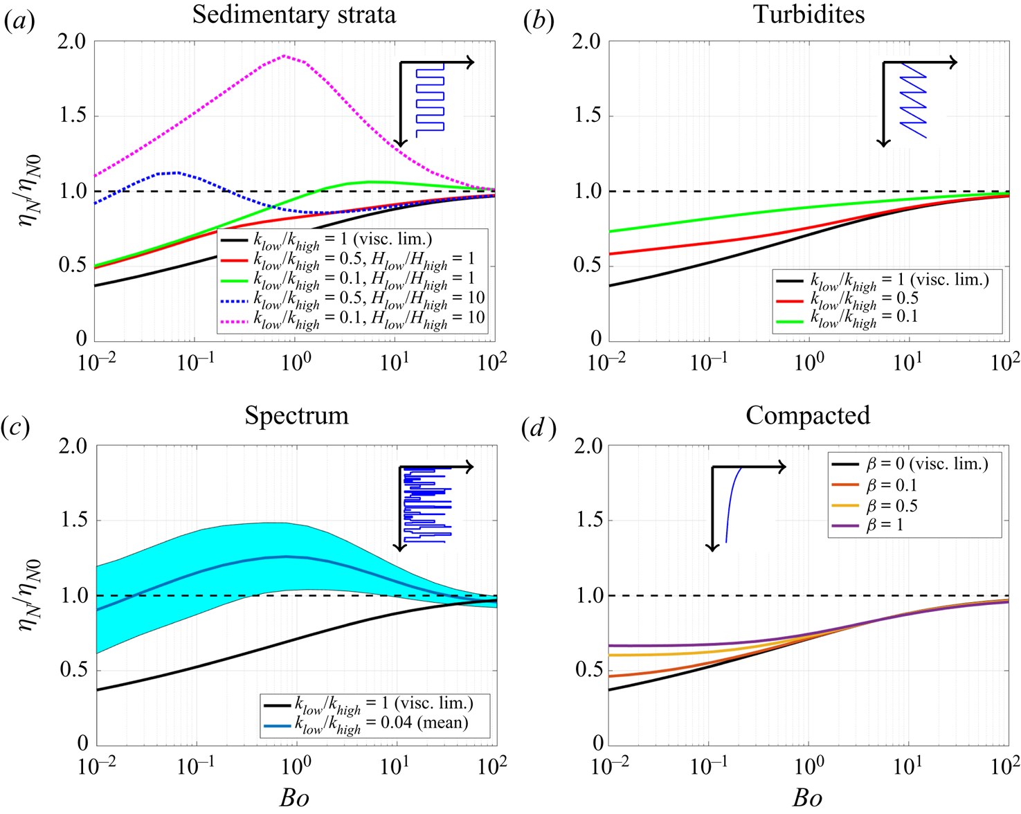
Mid-range thickness of the gravity current  $h_{half}=h(\eta _N/2)$, given in terms of the single-phase limit $h_{{half}_0}=0.348H$ for the non-compacted cases (a) and the compacted case (b). Limiting behaviours are illustrated with dashed lines.

In the limit  $Bo\ll 1$ the mid-range thickness $h_{half}$ behaves similarly for all non-compacted cases, growing approximately like $h_{half}\sim Bo^{-1/2}$, as described by Golding et al. (Reference Golding, Huppert and Neufeld2013) for the homogeneous case. On the other hand, the prefactor $\eta _N$ behaves rather differently. In all cases, we see an increase in $\eta _N$ for stronger heterogeneities, indicating that capillary forces accelerate the gravity current. However, each heterogeneity affects the prefactor $\eta _N$ differently, as can be seen in the different shaped curves in figure 7. This reflects the complex nature of the velocity distributions and flux functions depicted in figures 3 and 11. It is interesting to note that despite having a permeability profile with the same mean value, the different variations within each layer for each heterogeneity type are sufficient to alter the flux of saturation, and, hence, modify the speed of propagation of the gravity current. This sheds light on both the need for detailed bore hole measurements to infer as much information about the heterogeneities as possible, as well as the usefulness of such an upscaling approach as we have taken here.
For each of the different types of strata, we compare the capillary limit curves against the homogeneous case (solid black line), which is equivalent to the viscous limit. This allows us to quantify the effect of the heterogeneities on the prefactor more clearly. The strongest effect on the prefactor occurs when there are thin regions of high permeability  $(H_{low}/H_{high}=10)$ in which the non-wetting saturation concentrates. This focusing of the saturation feeds into the nonlinearity of the relative permeability, thereby amplifying the effect on the flux function $\mathcal {F}$. By contrast, thin regions of low permeability $(H_{low}/H_{high}=0.1)$ produce results which are very close to the homogeneous case, so we do not display them here.
In the case of the permeability spectrum, we choose a permeability distribution whose standard deviation divided by the mean is  $\sigma (k)/k_0=1$, and whose mean permeability ratio (between lowest and highest values) is $\mu (k_{low}/k_{high})=0.04$. The standard deviation is chosen to represent moderately heterogeneous media, as opposed to extremely heterogeneous media ( $\sigma (k)/k_0>1$), according to the criteria laid out by Corbett & Jensen (Reference Corbett and Jensen1992) and Martinius et al. (Reference Martinius, Ringrose, Næss and Wen1999). Likewise, the permeability ratio between layers $k_{low}/k_{high}$ is consistent with moderate to extreme permeability variations, and indeed similar (e.g. two orders of magnitude) variations have been observed in Salt Creek, USA (Bickle et al. Reference Bickle, Kampman, Chapman, Ballentine, Dubacq, Galy, Sirikitputtisak, Warr, Wigley and Zhou2017), Goldeneye field, North Sea (Jackson & Krevor Reference Jackson and Krevor2020) and in the Tilje formation in Norway (Martinius et al. Reference Martinius, Ringrose, Næss and Wen1999).
We calculate the prefactor  $\eta _N$ for 50 different realisations of this distribution and plot the results in figure 7(c). For each Bond number, we display the mean value, as well as one standard deviation on either side $\mu (\eta _N)\pm \sigma (\eta _N)$. The mean result is reminiscent of the previous sedimentary strata cases. However, it is interesting to note that the standard deviation is largest for a low-medium Bond number and shrinks as the Bond number gets larger. Hence, predictions are particularly prone to uncertainty if the Bond number is less than order unity. For $\textrm {CO}_{2}$ sequestration applications, this indicates that particular attention towards measurements of heterogeneities should be paid for injection sites with low flow rates (see discussion at the end of this section).
Next, we move on to describe the compacted case in the capillary limit (figure 6b,d,f). The presence of compaction is most noticeable in the small Bond number cases. By comparing figures 6(b) and 6(a), we see that compaction significantly increases the saturation within the gravity current, which is due to the permeability gradient forcing the non-wetting phase upwards. This is accompanied by an increase in the prefactor  $\eta _N$ and a decrease in $h_{half}$, as seen in figures 7(d) and 8(b). This is expected since, if a larger saturation is maintained, mass conservation indicates that the gravity current must be thinner. By varying the compaction power law $\beta$ from 0 to 1, we illustrate a fairly uniform transition of the values of $\eta _N$ and $h_{half}$ between those of a uniform rock and those of a strongly compacted rock.
For  $Bo\gg 1$, the saturation becomes near uniform $s\approx 1$, as before, and this is accompanied by both $\eta _N$ and $h_{half}$ converging to their single-phase limits. Hence, at such large Bond numbers the effect of compaction on the saturation distribution and gravity current shape is not particularly noticeable. This is expected, since compaction forces the saturation upwards, just like gravity.
For applications to  $\textrm {CO}_{2}$ storage, it is useful to infer from the above results how much we can expect heterogeneities to affect the speed of propagation of a gravity current. Such information allows one to make efficiency predictions for $\textrm {CO}_{2}$ storage that help pinpoint the best sites for injection, as well as safety predictions that ensure the $\textrm {CO}_{2}$ does not spread beyond the desired perimeter. Using the homogeneous case, $k_{low}/k_{high}=1$ (which is equivalent to the viscous limit), as the base case, we define the efficiency parameter $\nu$ as the relative difference we can expect heterogeneities to make on the prefactor $\eta _N$, such that
 \begin{equation} \nu({Bo},k(z))= \left[{\eta_{N_{het}}}/{\eta_{N_{hom}}}-1\right]\times 100\,\%.\end{equation}
Clearly  $\nu$ depends on a number of parameters, but here we focus on the different types of heterogeneity $k(z)$ and the Bond number. Restricting our attention to the layered cases (ignoring compaction), we plot the heterogeneity efficiency $\nu$ in figure 9 for different values of the Bond number. The largest heterogeneity efficiency is observed for the sedimentary strata with thin bands of high permeability ( $H_{low}/H_{high}=10$). As we mentioned earlier, this can be explained by a nonlinear focusing of the saturation into these high-speed bands. The most we can expect heterogeneities to accelerate the gravity current at high Bond number is around $\nu =10 - 50\,\%$, whereas at low Bond number the speedup can be as much as $\nu =100 - 200\,\%$. In the case of the permeability spectrum we also illustrate the standard deviation of the predictions, indicating that the results are particularly sensitive to uncertainty at low Bond number.
Heterogeneity efficiency  $\nu$ (3.1), describing the relative increase in prefactor value $\eta _N$ due to heterogeneities, given as a ratio of the prefactor value for the homogeneous case. Here we focus on the layered cases (S.S. stands for sedimentary strata), ignoring compaction. In the case of the permeability spectrum we plot the mean value as well as one standard deviation on either side. The permeability ratio for all cases is $k_{low}/k_{high}=0.04$. An arrow illustrates how the Bond number may decrease over time in post-injection scenarios (as the plume thins out).
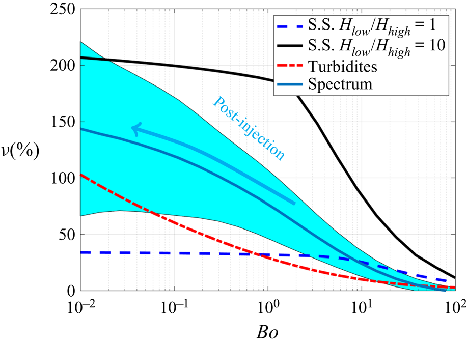
It is interesting to note that whilst fluid is injected at constant flow rate  $Q$, the Bond number is held constant, but if the flow were to stop suddenly this would no longer be the case. In such situations, the buoyancy length scale $H=\sqrt {Q/u_b}$, which was previously used to define the Bond number, would be rendered meaningless. Instead, the appropriate length scale for the flow would be the gravity current thickness itself $h$ which, after the cessation of $Q$, would gradually decrease towards zero (see discussion in the conclusion). Hence, the Bond number of the flow would decrease accordingly, as illustrated in figure 9, causing the effect of the heterogeneities to be increasingly amplified with time.
This is particularly relevant for  $\textrm {CO}_{2}$ storage applications, where the injection of gas is switched off once the aquifer is deemed to have reached maximum safe capacity. Hence, in such situations, it is clear that modelling heterogeneities is essential for understanding the post-injection spread of the $\textrm {CO}_{2}$. However, it is important to note that such situations involve imbibition flows, as opposed to drainage flows, as we have studied here (Woods Reference Woods2015). Imbibition flows typically have different capillary pressure and relative permeability curves than drainage flows, though the approach studied here is still applicable. Furthermore, we note that even in such situations the leading edge of the plume is still a drainage flow.
It is also useful to note here the typical ranges of Bond numbers for different carbon sequestration sites. To do so, we take upper and lower bound estimates for the gravity current thickness scale  $H=1 - 10\ \mathrm {m}$, the density difference $\Delta \rho =232 - 440\ \textrm {kg}\ \textrm {m}^{-3}$ and the pore entry pressure $p_{0}=1.3 - 493.6$ kPa (Bennion & Bachu Reference Bennion and Bachu2006; Golding et al. Reference Golding, Neufeld, Hesse and Huppert2011; Cowton et al. Reference Cowton, Neufeld, White, Bickle, White and Chadwick2016; Williams & Chadwick Reference Williams and Chadwick2017). Hence, the Bond number $Bo=\Delta \rho g H/p_{0}$ is in the range $0.005< Bo<35$. This indicates that the effects we observe at low Bond number are relevant for many carbon sequestration sites, indicating the need for careful upscaled modelling and detailed heterogeneity measurements. In the next section we show that several useful analytical results can be derived in the limit of large and small parameter values using asymptotic analysis.
3.2. Limiting cases and analytical solutions
Some simplifications can be made in the limits of strong and weak capillary forces (i.e. small and large Bond numbers). Here we address these and derive analytical solutions which we use to explain some of our earlier numerical results. We split the analysis into situations without compaction  $\beta =0$ and with compaction $\beta >0$. As in the previous section, here we restrict our attention to viscous limit and capillary limit behaviour only.
3.2.1. Weak capillary forces without compaction
We already showed earlier that in the limit of a large Bond number the saturation distribution (2.27) is approximately uniform  $s\approx 1$. Inserting this into the integrals (2.15), (2.18), we see that
 $$\begin{gather} \mathcal{S}\approx\varphi h, \end{gather}$$
 $$\begin{gather}\mathcal{K}\approx k_0 k_{rn0} h, \end{gather}$$
which allows us to calculate the dimensionless flux
 \begin{equation} \hat{\mathcal{F}}=\hat{f}.\end{equation}
This linear power law matches with our numerical observations in figure 3(c). Comparing (3.2), (3.4) with the study by Lyle et al. (Reference Lyle, Huppert, Hallworth, Bickle and Chadwick2005), we see that the limit of a large Bond number is identical to the classic single-phase limit. This is of course expected, since in the limit of weak capillary forces the flow of phases decouples, such that a single-phase model becomes appropriate. This explains the convergence behaviour for both  $\eta _N$ and $h_{half}$ for $Bo\gg 1$, as we illustrate with dashed lines in figures 7 and 8.
3.2.2. Strong capillary forces without compaction
To address the limit of strong capillary forces, we first consider the homogeneous case  $k_{low}/k_{high}=1$ (equivalent to the viscous limit) since this makes the analysis for the subsequent heterogeneous cases easier. Hence, in the limit of small $Bo\ll 1$ in the homogeneous case, the saturation distribution (2.12) approximates to a linear function
 \begin{equation} s\approx\lambda Bo \frac{(h-z)}{H}.\end{equation}
Inserting this into the integrals (2.15), (2.18) we get
 $$\begin{gather} \mathcal{S}\approx\frac{\varphi \lambda Bo }{2H}h^{2}, \end{gather}$$
 $$\begin{gather}\mathcal{K}\approx \frac{k_0k_{rn0}H\lambda^{\alpha} Bo^{\alpha} }{\alpha+1}\left(\frac{h}{H}\right)^{\alpha+1}, \end{gather}$$
from which we calculate the dimensionless flux
 \begin{equation} \hat{\mathcal{F}}=\left[\frac{2^{\alpha/2}(\lambda Bo)^{\alpha/2-1}}{\alpha+1}\right]\hat{f}^{\alpha/2} .\end{equation}
In this case, the flux has an  $\alpha /2$ power law, which matches with our numerical calculations in figure 3(a) (for which $\alpha =4$). The gravity current thickness is given by inverting (3.6), such that
 \begin{equation} h= H\left({2\hat{f}}/{\lambda Bo}\right)^{1/2}.\end{equation}
Clearly, the thickness grows like  $h\sim Bo^{-1/2}$ as $Bo\rightarrow 0$, which we illustrate in figure 8 with dashed lines. Our numerical results show good agreement, indicating their robustness. We also note that the square root in (3.9) explains why we see a blunting of the gravity current nose at low Bond numbers in figures 5 and 6.
If we now consider a finite heterogeneity  $k_{low}/k_{high}<1$, then in the case of sedimentary strata, the saturation distribution takes one of two possible values,
 \begin{equation} s\approx \begin{cases} 0: & k=k_{low},\\ \lambda Bo {(h-z)}/{H}: & k=k_{high}. \end{cases}\end{equation}
Since the low/high permeability layers are distributed according to the ratio  $H_{low}/H_{high}$, the integrals (2.15), (2.18) approximate to
 $$\begin{gather} \mathcal{S}\approx\left(\frac{H_{high}}{H_{high}+{H_{low}}}\right)\left(\frac{k_{high}}{k_0}\right)^{a}\frac{\varphi \lambda Bo}{2H}h^{2}, \end{gather}$$
 $$\begin{gather}\mathcal{K}\approx \left(\frac{H_{high}}{H_{high}+{H_{low}}}\right)\frac{k_{high}k_{rn0}H\lambda^{\alpha} Bo^{\alpha} }{\alpha+1}\left(\frac{h}{H}\right)^{\alpha+1}. \end{gather}$$
Hence, the dimensionless flux is
 \begin{equation} \hat{\mathcal{F}}=\left[\left(\frac{H_{high}}{H_{high}+{H_{low}}}\right)^{\alpha/2}\left( \frac{k_{high}}{k_0}\right)^{1-a(1+\alpha/2)}\frac{2^{\alpha/2}(\lambda Bo)^{\alpha/2-1}}{\alpha+1} \right]\hat{f}^{\alpha/2}.\end{equation}
Like the homogeneous case, the heterogeneous flux has an  $\alpha /2$ power law, which also matches with our numerical calculations for sedimentary strata in figure 3(a) (for which $\alpha =4$). We note that in the above analysis, the saturation approximation (3.10), and consequently the flux (3.13), are only valid for heterogeneities which have a small enough permeability ratio that $(1-k_{low}/k_{high})/(1+k_{low}/k_{high})\gg Bo$. However, for this study, we restrict our attention to significantly heterogeneous media (rather than weakly heterogeneous).
We also note that in both the homogeneous case and the heterogeneous case, the coefficients in (3.8), (3.13) depend on the Bond number itself. Therefore, we do not expect a constant value asymptote for the prefactor  $\eta _N$ in the limit $Bo\rightarrow 0$ (except in the specific case $\alpha =2$), which is consistent with our numerical observations in figure 7.
In the case of the permeability spectrum, a similar analysis is possible since the only contribution to the integrals will come from the regions with the largest permeability value  $k=k_{high}$. However, since there are potentially many more than just two permeability values in the spectrum, one needs to replace the factor $H_{high}/(H_{high}+{H_{low}})$ in (3.11)–(3.13) with the fraction of the aquifer occupied by such high permeability layers, which we denote $H_{high}/H_{total}$. In the case of the turbidites, a similar analysis to the above is much more difficult, since we cannot approximate the saturation distribution as simply as (3.10).
It is important to briefly discuss the case where there is no gravity. For example, a previous study (Benham et al. Reference Benham, Bickle and Neufeld2021) addressed the effects of heterogeneities on fluid displacement in a long-thin confined aquifer (also known as a Buckley–Leverett flow), for which gravity is negligible. However, it is not possible to make a direct analogy here, since the flow of the ambient phase is neglected in the present study (because the current is unconfined). Indeed, our model formulation does not permit a complete removal of the gravitational force, since we have neglected pressure gradients due to injection which would otherwise drive the flow. Nevertheless, the expressions (3.8) and (3.13) represent the limiting behaviour as gravity becomes vanishingly small compared with capillary forces. Hence, to isolate the individual effects of gravity and capillary forces, it is sufficient to compare (3.4) to (3.8) and (3.13) (and, more usefully, the resulting prefactors  $\eta _N$ which determine plume migration speeds).
3.2.3. Weak capillary forces with compaction
In the case where the rock is compacted, the saturation (2.27) must be approximately uniform  $s\approx 1$ in the limit of a large Bond number, as before. Inserting this into the integrals (2.15), (2.18), we see that
 $$\begin{gather} \mathcal{S}\approx\varphi H \frac{(1 + h/H)^{1-a \beta} - 1}{1 - a \beta}, \end{gather}$$
 $$\begin{gather}\mathcal{K}\approx k_0 k_{rn0} H\frac{(1 + h/H)^{1- \beta} - 1}{1 - \beta}. \end{gather}$$
Note that if either  $\beta$ or $a\beta$ equals unity, we get analytical expressions with logarithms instead of (3.14), (3.15). Assuming that $\beta \neq 1$, $a\beta \neq 1$, we then calculate the dimensionless flux, which we write in terms of $h$ for now,
 \begin{equation} \hat{\mathcal{F}}=\frac{(1 + h/H)^{\beta(a-1)+1} -(1+h/H)^{ a\beta}}{1 - \beta}.\end{equation}
Clearly the flux (3.16) is not a linear function of  $\mathcal {S}$ (3.14) as in the homogeneous case. However, we note that for weak porosity–permeability power laws $a\ll 1$ (e.g. $a=0.14$ for the Salt Creek case study, Bickle et al. Reference Bickle, Kampman, Chapman, Ballentine, Dubacq, Galy, Sirikitputtisak, Warr, Wigley and Zhou2017) the integrated saturation (3.14) approximates to a linear function $\mathcal {S}\approx \varphi h$, as we observe in our numerical calculations in figure 11(e). Furthermore, in situations where the compaction law is weak $\beta \ll 1$, or alternatively where the gravity current thickness is small ${h}/H\ll 1$, the flux (3.16) reduces to $\hat {\mathcal {F}}\approx {h}/H$, thereby recovering the single-phase limit (3.4). This is in accordance with our numerical observations in figure 3(c).
However, we note that by choosing sufficiently strong compaction/porosity power laws  $a,\beta$, the single-phase limit is no longer recovered in the limit of a large Bond number. Physically speaking, this is because even with weak capillary forces, if the medium is sufficiently compacted the velocity distribution within the gravity current becomes dominated by the permeability variation, which upon integration creates a flux power law that is not equal to one.
3.2.4. Strong capillary forces with compaction
To address the compacted case at small Bond number, we first consider the form of the saturation (2.10). In particular, we note that since  $k$ is monotone decreasing with depth, the saturation $s$ is also monotone decreasing. In particular, we can calculate that $s$ will intercept zero at some depth $z^{*}$ which satisfies $\Delta \rho g (h-z^{*})+p_0=p_e(z^{*})$, and will remain zero for all larger depths than this $z>z^{*}$. Therefore, without loss of generality, we take $p_0=p_e(h)$, such that there are no regions of zero saturation within the gravity current. In this way, for a small Bond number, (2.10) approximates to a finite expression which is independent of $Bo$,
$Bo$,
 \begin{equation} s\approx 1-\left(\frac{1+z}{1+h}\right)^{\lambda \beta b }.\end{equation}
This explains why the properties of the gravity current (e.g.  $\eta _N,h_{half}$) asymptote to constant values for $Bo\rightarrow 0$ in figures 7(d) and 8(b). For general power laws $a,b,\lambda ,\alpha ,\beta$, inserting (3.17) into the integrals (2.15), (2.18) leads to very complicated analytical expressions, which we do not display here. As we can see in figure 3(a), the flux for this case does not obey a fixed power law, but the exponent varies roughly between 1 and 2.
The power law of the flux function can be roughly interpreted as the amount of distortion that heterogeneities cause on the velocity within the gravity current (e.g. via the relative permeability and capillary pressure). Hence, a power law which varies between 1 and 2 as the saturation varies can be interpreted as follows. In the thin part of the gravity current (small  $\mathcal {S}$) compaction distorts the flow more (power law closer to 2), whereas in the thick part (large $\mathcal {S}$) it distorts the flow less (power law closer to 1). This can be explained by the fact that the compaction profile $k(z)$ (see table 1 or figure 2g) has the largest gradient near $z=0$.
3.3. Viscous-capillary transition
Up until now we have only discussed situations where the capillary number (2.20) is either very large (viscous limit), in which capillary forces due to heterogeneities can be ignored (i.e. effectively the homogeneous case), or very small (capillary limit), in which the heterogeneities play a dominant role on the flow behaviour (i.e. the heterogeneous cases studied above). However, in general, the capillary number may vary between small and large values throughout the aquifer. In this case, neither the viscous nor the capillary limit can be applied to the flux function in (2.16), and instead the flux must depend on the local capillary number, which is effectively a measure of the local pressure gradients within the gravity current. In this section we discuss how to model this using numerical simulations of the full PDE (2.16) coupled to the transcendental equation (2.20), thereby determining which regions of the gravity current are within the viscous and capillary limits, and which regions lie in between these limits.
Following the same approach as Benham et al. (Reference Benham, Bickle and Neufeld2021), we formulate composite functions for the upscaled properties of the flow, which capture both the viscous and capillary limit regimes, as well as the transition between these limits. The two upscaled quantities of interest are the integrated saturation  $\mathcal {S}$ and the flux $\mathcal {F}$. For each of these upscaled quantities $\{\mathcal {S},\mathcal {F}\}$, the transition behaviour is given in terms of the mean saturation (2.13) and capillary number (2.20) by the formula
 \begin{equation} \left\{\mathcal{S},\mathcal{F}\right\}_{{trans}}=\frac{1}{2}\left[ \left\{\mathcal{S}(\bar{s}),\mathcal{F}(\bar{s})\right\}_{-} \tanh \left(\frac{\log{{N}_c}-\log{{N}_{c_t}}}{\log \varDelta}\right)+\left\{\mathcal{S}(\bar{s}),\mathcal{F}(\bar{s})\right\}_{+}\right],\end{equation}
where  $\{\mathcal {S},\mathcal {F}\}_{\pm }=\{\mathcal {S},\mathcal {F}\}_{{visc}}\pm \{\mathcal {S},\mathcal {F}\}_{{cap}}$ is given in terms of the viscous limit (homogeneous) and capillary limit (heterogeneous) upscaled properties derived earlier, and $N_{c_t}$, $\varDelta$, are two fitting parameters which represent the transition capillary number and folding scale, respectively. The precise values of these fitting parameters depend on numerous factors, including the type of heterogeneity and the specific power laws used, but here we use the same values as calculated by Benham et al. (Reference Benham, Bickle and Neufeld2021), which are $N_{c_t}= 394$, $\varDelta =5.5$, and these were shown to give good comparison with numerical simulations across a large range of capillary numbers with a mean relative error of ${\sim }1\,\%$.
By accounting for the dependence of the upscaled flux on the capillary number, the system loses its self-similarity. In mathematical terms, this can be seen by noticing that the capillary number (2.20) in the governing equation (2.16) contains derivatives of  $\mathcal {S}$ with respect to $r$, compromising the self-similar structure of the equations. Therefore, since we are no longer able to convert to a single governing similarity ODE, we must instead solve the full PDE (2.16) numerically, in conjunction with the algebraic equation for the capillary number (2.20). Written in dimensionless terms, we observe that the capillary number is related to the Bond number according to
 \begin{equation} {N}_c=\frac{Bo p_0}{\Delta p_e}\left|\frac{h(\mathcal{S},{N}_c)/H}{\mathcal{S}_h(h(\mathcal{S},{N}_c),{N}_c)}\frac{\partial \mathcal{S}}{\partial r}\right|.\end{equation}
For the sake of the calculations in this section, we use a mid-range value of  $Bo=1$ for the Bond number, since this represents an even balance between capillary and gravity forces.
In figure 10 we display the numerical solution in the case of sedimentary strata ( $k_{low}/k_{high}=1/3,H_{low}/H_{high}=1$), plotted at three different times after injection, illustrating the evolution of the gravity current, as well as the spatial variation in the local capillary number (3.19). At all times the gravity current has a region which is in the capillary limit, a region which is in the viscous limit and a region which is in a transition regime. At early times most of the gravity current lies within either the viscous limit or a transition regime, whereas the very tip of the nose lies in the capillary limit. Indeed, the nose of the gravity current lies in the capillary limit for all times, since the flux vanishes there (since $N_c\sim h\partial p_n/\partial r\sim h\partial h/\partial r\rightarrow 0$ as $r\rightarrow r_N(t)$ due to (2.22)). At later times a substantial portion of the gravity current lies within the transition regime, with the near-origin and near-nose regions remaining in the viscous and capillary limits, respectively. The position of the nose of the gravity current $r_N(t)$ is plotted on a logarithmic scale in figure 10(g), also indicating the viscous and capillary limit curves.
Numerical solution of the evolution of the gravity current (2.16), accounting for transition behaviour between viscous and capillary limits using composite expressions (3.18) for the upscaled flow properties, where the capillary number is given implicitly by (3.19) (with  $Bo=1$). The gravity current shape, shaded to illustrate the saturation distribution (using the same colour scale as in figures 5 and 6), is illustrated in (a–c), whereas the local capillary number $N_c$ is illustrated in (d–f). For all plots, we shade regions with capillary number one folding scale larger than the transition value $N_c>N_{c_t}\times \varDelta =2167$ in green, and regions with one folding scale smaller $N_c< N_{c_t}\times \varDelta ^{-1}=72$ in blue. The transition capillary number $N_{c_t}$ is illustrated with a dashed red line within a white region, indicating a transition regime. The evolution of the gravity current nose position $r_N(t)$ is shown on a log-log plot in (g).

We make several observations. Firstly, we note the dynamic transition between viscous-like behaviour at early times and capillary-like behaviour at late times. This is evident from figure 10(g), where we see that the nose position initially grows like  $\sim t^{1/2}$ with a prefactor corresponding to the viscous limit, and later grows like ${\sim } t^{1/2}$ with a capillary limit prefactor. There is a transition period at intermediate times where the behaviour does not obey a power law (as observed by Benham et al. (Reference Benham, Bickle and Neufeld2021) in the absence of gravity). This can be explained by the fact that, as the gravity current spreads out radially, the capillary number reduces everywhere except near the origin (where $N_c\rightarrow \infty$). In this way, the composite expressions (3.18) in the majority of the gravity current switch between viscous limit behaviour to capillary limit behaviour over time. Secondly, we note that since the viscous-capillary transition point ( $N_c=N_{c_t}$) tends to a constant position ( $r/H\approx 0.2$) over time, if we continue the simulation indefinitely, the fraction of the gravity current in the capillary limit tends towards unity, indicating that at late times ( $tu_b/H\gg 1$) a capillary limit model is a good approximation for the whole aquifer.
4. Discussion of applications to  $\textrm {CO}_{2}$ sequestration

In this section we discuss the implications of the upscaled description of gravity currents in the context of  $\textrm {CO}_{2}$ sequestration. There are many different sites that we could choose as case studies, but probably the one with the most available data is at the Sleipner project in the North Sea (Bickle et al. Reference Bickle, Chadwick, Huppert, Hallworth and Lyle2007). In particular, we focus on the top layer, which has been investigated by numerous authors (Chadwick, Noy & Holloway Reference Chadwick, Noy and Holloway2009; Williams & Chadwick Reference Williams and Chadwick2017). Whilst various attempts have been made to model the $\textrm {CO}_{2}$ migration at Sleipner, and comparisons have been made with seismic measurements of the extent of the plume (Bickle et al. Reference Bickle, Chadwick, Huppert, Hallworth and Lyle2007; Golding et al. Reference Golding, Huppert and Neufeld2013; Cowton et al. Reference Cowton, Neufeld, White, Bickle, White and Chadwick2016, Reference Cowton, Neufeld, White, Bickle, Williams, White and Chadwick2018), these attempts have often fitted certain parameters (e.g. the permeability) to match observations, without accounting for the possible effect of heterogeneities. Therefore, here we use our previous upscaling procedure to perform this analysis, calculating the effect that different types of heterogeneities could have had on plume migration speeds. Since little is known about the geological heterogeneities at Sleipner, we investigate all the different types of layering we studied earlier, and we account for how uncertainty in such layering may propagate to uncertainty in the modelling predictions.
As described earlier in § 2.3, there are eight non-dimensional parameters in our model (excluding the capillary number). Of these parameters, five relate to the type of heterogeneities, about which little is known for Sleipner. Therefore, instead we take the following values from other similar studies: the porosity–permeability power law used by Bickle et al. (Reference Bickle, Kampman, Chapman, Ballentine, Dubacq, Galy, Sirikitputtisak, Warr, Wigley and Zhou2017)  $a=1/7$; the pore entry pressure power law taken from the scaling proposed by Leverett (Reference Leverett1941) $b=3/7$; the permeability ratio taken from Bickle et al. (Reference Bickle, Kampman, Chapman, Ballentine, Dubacq, Galy, Sirikitputtisak, Warr, Wigley and Zhou2017) $k_{low}/k_{high}=0.01$, no compaction $\beta =0$, and we vary the layer ratio $H_{low}/H_{high}$ between $1$ and $10$. Since it is unknown whether sedimentary strata, turbidites or a permeability spectrum is most appropriate, we investigate all of these different heterogeneity types.
There are two parameters relating to the multiphase flow properties  $\lambda$ and $\alpha$, which define the capillary pressure and relative permeability. We note that not all relative permeability curves are parameterised as simply as (2.5). For example, other more nonlinear functional forms have been proposed by Chierici (Reference Chierici1984). However, we note that Chadwick et al. (Reference Chadwick, Noy and Holloway2009), Williams & Chadwick (Reference Williams and Chadwick2017) use the Brooks–Corey formulation to model Sleipner, which is given by
 \begin{equation} k_{rn}=k_{rn0}s^{2}\left[1-(1-s)^{2}\right].\end{equation}
We could change our formulation to account for this modified parameterisation, but instead we notice that (4.1) can be approximated by (2.5) with mean relative error  $3\,\%$ using a power law value of $\alpha =2.32$. Therefore, we stick with our original formulation (2.5) for the sake of consistency, without sacrificing much accuracy. Meanwhile, the pore size distribution is estimated by Chadwick et al. (Reference Chadwick, Noy and Holloway2009) as $\lambda =2/3$.
The final parameter we need to describe the problem is the Bond number, which is defined by (2.26) in terms of six other physical parameters (excluding gravity,  $g=9.81\ \textrm {m}\ \textrm {s}^{-2}$). For the top layer at Sleipner, Williams & Chadwick (Reference Williams and Chadwick2017) estimate the temperature between $28 - 31\,^{\circ }\textrm {C}$ and pressure between 8.2–8.9 MPa, which gives a density difference of $\Delta \rho =232 - 309\ \textrm {kg}\ \textrm {m}^{-3}$. Meanwhile, the viscosity of $\textrm {CO}_{2}$ is taken as $\mu _n=54.7 - 65.5\times 10^{-6}\ \textrm {Pa}\ \textrm {s}$. The input flux is best estimated by Cowton et al. (Reference Cowton, Neufeld, White, Bickle, White and Chadwick2016), which for the first few years of injection is $Q=1.5 - 3\times 10^{-3}\ \textrm {m}^{3}\ \textrm {s}^{-1}$. The mean permeability is estimated by Bickle et al. (Reference Bickle, Chadwick, Huppert, Hallworth and Lyle2007) as $k_0=1.1 - 5\times 10^{-12}\ \textrm {m}^{2}$. Finally, the pore entry pressure and end-point relative permeability are given by Williams & Chadwick (Reference Williams and Chadwick2017) as $p_0=1.3$ kPa and $k_{rn0}=0.28$. Putting these all together, we estimate the Bond number as $Bo=8.9 - 35.5$. Hence, Sleipner, being a very permeable reservoir, lies towards the upper end of the range of Bond numbers for carbon sequestration applications (see discussion at the end of § 3.1). Consequently, heterogeneities in other sites are likely to accelerate plume migration by an even larger factor than we calculate here.
Now that we have determined all the parameter values (up to a given uncertainty), we follow the procedure outlined earlier to calculate the prefactor  $\eta _N$ for the gravity current using the various different heterogeneity types. In this way, we can measure the heterogeneity efficiency $\nu$ (3.1), which tells us how much we can expect the heterogeneities to modify the speed of propagation. In the low/high Bond number estimate $Bo=8.9/35.5$, we find that $\nu =36\,\%/31\,\%$ for equally distributed sedimentary strata ( $H_{low}/H_{high}=1$), $\nu =147\,\%/108\,\%$ for sedimentary strata with thin streaks of high permeability ( $H_{low}/H_{high}=10$), $\nu =11\,\%/6\,\%$ for turbidites, and $\nu =23\pm 11\,\%/9\pm 8\,\%$ for a permeability spectrum. In the latter case, we include the standard deviation values to indicate how these predictions vary due to the uncertainty of the heterogeneity measurements. Indeed, the large degree of uncertainty in these predictions not only illustrates the need for more detailed bore hole measurements at Sleipner, but also demonstrates the importance of accounting for such uncertainty in any modelling approach.
We note that the permeability ratio in the Sleipner field may not be as small as the value we have taken from Salt Creek,  $k_{low}/k_{high}=0.01$ (Bickle et al. Reference Bickle, Kampman, Chapman, Ballentine, Dubacq, Galy, Sirikitputtisak, Warr, Wigley and Zhou2017). Therefore, we also perform the same analysis as above using a permeability ratio ten times larger. We find that the efficiencies $\nu$ calculated for $k_{low}/k_{high}=0.1$ are between $1/5$ and $3/5$ of their values for $k_{low}/k_{high}=0.01$. This indicates that, even if we have vastly overestimated the permeability ratio, the effect of heterogeneities is still likely to be significant.
From this analysis, it is clear that the possible effect that heterogeneities may have had on the injection of  $\textrm {CO}_{2}$ at Sleipner largely depends on the type of heterogeneities present. In particular, thin sedimentary strata with very high permeability could have caused a potential speedup of more than $100\,\%$. However, for more moderate permeability profiles, such as evenly distributed strata or turbidites, these heterogeneities may have only caused a 10–30 % speedup.
5. Concluding remarks
We have studied the upscaled effect of several different types of heterogeneity on the evolution of an axisymmetric gravity current under an impermeable cap rock. The four heterogeneity types considered, which were all given in terms of vertical variations in the rock properties, were each motivated by different physical mechanisms for the non-uniform deposition or compaction of sediments. We developed a general method for calculating the gravity current shape and growth rate in either the viscous or capillary limits, which involves solving a single similarity equation that depends on an upscaled flux term evaluated either via numerical integration, or using analytical expressions which we derived in certain limiting cases. This simplified approach not only greatly reduces computation time, but also provides key insights into the role of small-scale heterogeneities on the propagation of the large-scale flow.
In particular, we showed that heterogeneities have the ability to significantly accelerate plume migration due to the effects of relative permeability and capillary pressure. Indeed, the observed speedup is a consequence of the combined effect of both of these multiphase properties, with capillary pressure acting to focus the saturation into high permeability layers according to (2.10), and relative permeability acting to enhance the flow of saturation within these layers. The degree of speedup depends on the type of heterogeneity, and most importantly, the fraction of high/low permeability regions within the medium. The largest effect (e.g. 200 % faster) was seen in the case of sedimentary strata with thin regions of high permeability. Using a permeability profile composed of randomly sampled layers, we demonstrated how uncertainty in heterogeneity measurements can propagate to uncertainty in field predictions, an effect which is particularly pronounced for small values of the Bond number. We also investigated modelling the transition from the viscous limit regime to the capillary limit regime, shedding light into which regions of the gravity current are most affected by heterogeneities, and when.
The main motivation for this study was to create an upscaled description of how small-scale heterogeneities affect large-scale  $\textrm {CO}_{2}$ migration, for safe and efficient sequestration in porous aquifers. To assess the risks associated with any $\textrm {CO}_{2}$ storage scheme, examining the effect of heterogeneities is essential. To illustrate this, we used the case study of $\textrm {CO}_{2}$ injection at the Sleipner project in the North Sea. In this case, for realistic parameter values, we demonstrated that heterogeneities may have sped up the gravity current by more than 100 % during injection. However, we also illustrated that this figure depends greatly on the heterogeneity type, indicating the need for detailed core measurements from bore holes.
For future work, variations in the heterogeneities along the length of the aquifer could be studied (in addition to the vertical heterogeneities investigated here), similarly to Jackson & Krevor (Reference Jackson and Krevor2020). In such cases, the upscaled flow properties would depend on both the horizontal and vertical correlation length scales of the heterogeneities. In addition, using the upscaled results presented here, predictions of trapping efficiencies could be calculated for various sequestration sites. This could shed light onto which aquifers have heterogeneities that could potentially enhance their capability for  $\textrm {CO}_{2}$ storage. Furthermore, as we discussed earlier, it would be interesting to investigate the evolution of the gravity current after injection has stopped (see figure 9). To address this, one could consider the dynamics of a fixed volume of fluid $V$ spreading under gravity, for which the thickness scales approximately like $h\sim (V/u_bt)^{1/2}$. Hence, as $t\rightarrow \infty$, the Bond number scales like $Bo \sim \Delta \rho g/p_0(V/u_bt)^{1/2}\rightarrow 0$, and so we recover the small Bo limit post injection. However, to model this fully both imbibition and drainage relative permeability/capillary pressure curves must be considered, depending on whether the $\textrm {CO}_{2}$ is invading or being withdrawn from different regions of the aquifer, similarly to Golding, Huppert & Neufeld (Reference Golding, Huppert and Neufeld2017).
It would also be interesting to compare our predictions of the plume shape (e.g. figures 5 and 6) and velocity distribution (e.g. figure 11b,d,f) with either field or laboratory data. Such comparisons could be made possible with detailed measurements of subsurface geological heterogeneities in conjunction with tracer sampling (similar to Bickle et al. Reference Bickle, Kampman, Chapman, Ballentine, Dubacq, Galy, Sirikitputtisak, Warr, Wigley and Zhou2017), or with X-ray computerised tomography scans of injection into layered samples (similar to Jackson et al. Reference Jackson, Agada, Reynolds and Krevor2018).
(a,c,e) Variation of the integrated saturation  $\mathcal {S}$ (2.15) for different values of the Bond number Bo and different types of heterogeneity. Both $\mathcal {S}$ and $h$ are normalised by reference values (at $h=2h_{half}$) for illustration purposes. In each plot we indicate power law values of $1/2$, $1$,
$1$,  $2$ and $3$ with dotted lines for comparison. (b,d,f) Corresponding scaled velocity profiles $1-U=(u_n(0)-u_n(z))/(u_n(0)-u_n(h))$, where $u_n\propto \Delta \rho g k(z)k_{rn}(s)/\mu _n$. We plot the ensemble average of the velocity, rather than the velocity within each layer, so as not to display oscillatory behaviour between layers.
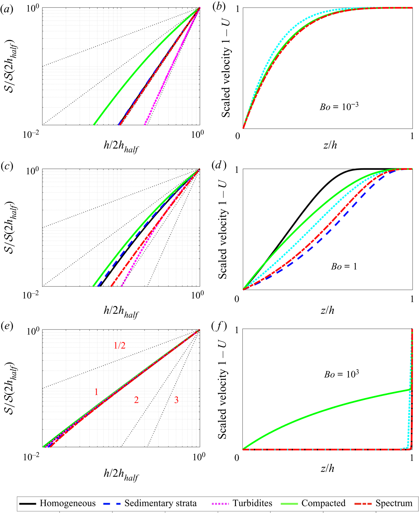
Supplementary material
Supplementary material is available at https://doi.org/10.1017/jfm.2021.523, which includes some code to numerically evaluate the flux integrals and calculate the similarity solution. This code can also be found on the personal website of G.P. Benham: https://yakari.polytechnique.fr/people/benham/gravity_current/upscale.m.
Funding
This research is funded in part by the GeoCquest consortium, a BHP-supported collaborative project between Cambridge, Stanford and Melbourne Universities, and by a NERC consortium grant ‘Migration of  $\textrm {CO}_{2}$ through North Sea Geological Carbon Storage Sites’ (grant no. NE/N016084/1).
Declaration of interests
The authors report no conflict of interest.
Appendix A. Extra plots
In this appendix we present extra plots in figure 11 for the integrated saturation  $\mathcal {S}$ (2.15) and the Darcy velocity of the non-wetting phase $u_n\propto \Delta \rho g k(z)k_{rn}(s)/\mu _n$ at different Bond numbers and for different types of heterogeneity.
The relationship between the integrated saturation  $\mathcal {S}$ and the gravity thickness $h$, as shown in figure 11(a,c,e), is useful for understanding how to invert the solution of the governing equation (2.16). In all cases $\mathcal {S}$ has approximate power law dependence on $h$, where the power is between linear and cubic, as illustrated with dotted lines.
The velocity profiles in figure 11(b,d,f) are useful for understanding the form of the flux function  $\mathcal {F}$ (which is the integrated velocity), as displayed in figure 3(a–c). We present the scaled velocity $1-U=(u_n(0)-u_n(z))/(u_n(0)-u_n(h))$ so that $U$ varies between $U=1$ at $z=0$ and $U=0$ at $z=h$. In this way we can see the functional form of $U$ more clearly. For example, if $U$ is constant (as in figure 11f), when integrated this will give a linear dependence between the flux $\mathcal {F}$ and the gravity current thickness $h$.
$h$.
Appendix B. Derivation of the governing equation (2.16)
In this appendix we provide the details for the derivation of the governing equation for the integrated saturation  $\mathcal {S}$, which is given by (2.16). We start by considering the governing equation for the gravity current thickness (2.14). To rewrite this in terms of the integrated saturation (2.15), we first need to transform the derivatives of $h$ into derivatives of $\mathcal {S}$. As illustrated by figure 11(a,c,e), the integrated saturation is always a monotone increasing function of the gravity current thickness, so that we can define a unique inverse function
 \begin{equation} h=\mathcal{S}^{{-}1}(\mathcal{S}).\end{equation}
Then, using the chain rule, the gradient is given by
 \begin{equation} \frac{\partial h}{\partial r} = \frac{\partial h}{\partial \mathcal{S}} \frac{\partial \mathcal{S}}{\partial r}. \end{equation}
We use the inverse derivative identity to calculate derivatives of (B1), such that
 \begin{equation} \frac{\partial h}{\partial \mathcal{S}} =\left(\frac{\partial \mathcal{S}}{\partial h} \right)^{{-}1}. \end{equation}
Finally, by defining the flux function  $\mathcal {K}$ as (2.18), we arrive at the governing equation for $\mathcal {S}$, which is
 \begin{equation} \frac{\partial \mathcal{S}}{\partial t} =\frac{u_b}{k_0k_{rn0}}\frac{1}{r}\frac{\partial}{\partial r}\left( r \left[\frac{\mathcal{K}}{\partial\mathcal{S}/\partial h}\right] \frac{\partial \mathcal{S}}{\partial r} \right). \end{equation}


 Open access