


Introduction
Lattice materials comprising periodic arrays of interconnected struts have emerged as a new class of engineering materials with potential for use in an incredibly diverse range of applications, including structural biomedical implants,[Reference Murr, Gaytan, Medina, Lopez, Martinez, Machado, Hernandez, Martinez, Lopez, Wicker and Bracke1–Reference Cheng, Li, Murr, Zhang, Hao, Yang, Medina and Wicker3] aerospace and naval structures,[Reference Evans, Hutchinson, Fleck, Ashby and Wadley4] force protection systems,[Reference Wadley5,Reference Chen, Barnhart, Chen, Hu, Sun and Huang6] thermal management,[Reference Wadley5] actuation,[Reference Lucato, Wang, Maxwell, McMeeking and Evans7–Reference Cramer, Cellucci, Olivia, Formoso, Gregg, Jenett, Kim, Lendraitis, Swei, Trinh, Trinh and Cheung9] high-performance running shoes,[Reference Bain10] and photonic and phononic crystals.[Reference Bückmann, Stenger, Kadic, Kaschke, Frölich, Kennerknecht, Eberl, Thiel and Wegener11,Reference Bauer, Hengsbach, Tesari, Schwaiger and Kraft12] They can be designed to exhibit unusual properties, including negative thermal expansion,[Reference Lakes13] negative Poisson's ratio,[Reference Evans and Alderson14] fluid-like elasticity (with an extraordinarily high ratio of bulk to shear moduli),[Reference Kadic, Buckmann, Stenger, Thiel and Wegener15] unusually high damping capacity,[Reference Ryan, Szyniszewski, Ha, Xiao, Nguyen, Sharp, Weihs, Guest and Hemker16] and negative mass density.[Reference Christensen, Kadic, Wegener and Kraft17] When the arrays are large, with individual unit cells being small relative to macroscopic length scales of interest, lattices can be treated effectively as other engineering materials in the sense that their properties can be couched in terms of their volume-averaged response to external stimuli. In establishing relationships between macroscopic properties and lattice structure, questions arise about the nature of structure of lattice materials and how characteristics of structure can be integrated into the materials science paradigm.
The field of materials science as an academic discipline is founded principally on relationships between processing, structure, and properties (Fig. 1). Here, structure encompasses the organization of atoms or molecules relative to one another, often in the form of crystals; boundaries between domains of differing orientation and/or composition; and defects that disrupt periodic arrangements at length scales ranging from the atomic to the macroscopic. Some of the important structural characteristics—including crystalline grains, grain and interphase boundaries, dislocations, precipitates, solute atoms, and vacancies—are depicted schematically in Figs. 2(a)–2(d). Although these characteristics are relevant to the constituent materials from which lattices are made, descriptions of the lattice structure itself require other concepts.
The traditional processing–structure–properties paradigm of materials science (in blue) is expanded to incorporate the structure and properties of lattice materials (in yellow).

Contrasting elements of structure and defects in traditional materials science and in lattice materials science. (a–d) Pertinent length scales in traditional materials science are well established: grains are typically 10–100 µm in size, precipitates 10–100 nm, dislocation spacings 10–100 nm, and solute atoms and vacancies at the sub-nm level. (e–o) Lattice structures and lattice defects are distinctly different from those in traditional materials science. Examples of low-order lattice topologies include (e) elementary cubic, (f) compound cubic, (g) super compound cubic, (h) the Kagome lattice, and (i) the diamond lattice. The Kagome structure, denoted  $\left\{ {R\left\lfloor {\matrix{ 0 & 0 & 0 \cr}} \right\rfloor \;\left\lfloor {\matrix{ {{1 / 2}} & 0 & 0 \cr}} \right\rfloor \;\left\lfloor {\matrix{ 0 & {{1 / 2}} & 0 \cr}} \right\rfloor \;\left\lfloor {\matrix{ 0 & 0 & {{1 / 2}} \cr}} \right\rfloor} \right\}$, is based on a rhombohedral space lattice in which the three interaxis angles are 60°; four nodes are assigned to each lattice point, at $\left\lfloor {\matrix{ 0 & 0 & 0 \cr}} \right\rfloor$, $\left\lfloor {\matrix{ {{1 / 2}} & 0 & 0 \cr}} \right\rfloor$, $\left\lfloor {\matrix{ 0 & {{1 / 2}} & 0 \cr}} \right\rfloor$ and $\left\lfloor {\matrix{ 0 & 0 & {{1 / 2}} \cr}} \right\rfloor$, and struts are placed between nearest-neighbor nodes. High-order lattices, based on (j) graded, (k) hierarchical, (l) and poly-topological designs, may provide access to property combinations not attainable with a single topology. (m) Defects include missing struts, shown here in the {FCC} structure and distinguished by their orientation relative to the loading direction. Type I struts are oriented perpendicular to the load axis, while types II and III are at 45° to the load axis. (n) Nodes and (o) external surfaces also constitute potential defects. Developments in node design and surface engineering will be required to mitigate effects of these features on lattice properties. (Features in (j–l) are represented by 2D schematics although they could be readily extended into 3D. Images in (e–i) reprinted from Ref. [Reference Zok, Latture and Begley18] and images in (m) reprinted from Ref. [Reference Latture, Begley and Zok19], with permission from Elsevier.)

The primary goal of this article is to present concepts of lattice structure that would expand the traditional processing–structure–properties paradigm and facilitate the study of lattice materials within a broader materials science framework. Some distinguishing characteristics of lattice materials and their structure–property relations are illustrated through examination of the internal response of lattice materials to external stress as well as the effects of external surfaces and defects (e.g., missing struts) on internal strains and failure initiation. Additionally, a case study is presented to illustrate how structure–property relations can be utilized in concurrent selection of topology, morphology, and constituent material in the design of strong lattice materials. Differences, commonalties, and analogies between elements of structure in the existing framework and those in lattice materials are highlighted throughout. Although the discussion of structure and defects presented here is largely in the context of mechanical properties (especially stiffness and strength), the concepts could be readily extended to other lattice properties.
The scope of the article is restricted largely to lattice materials that can be loosely characterized as being of “low order”. Although there is no formal definition of low order in the context of lattices, here it refers to systems that can be represented by a large number of relatively simple unit cells or representative volume elements with characteristic size scales that are much smaller than the dimensions of the entire lattice. High-order systems, on the other hand, include ones in which the largest characteristic length scale of the unit cell is comparable to the macroscopic lattice dimensions or in which the structure is spatially graded over macroscopic length scales.
The discussion of structure is further restricted to cases where the relative density of the lattice is small (say <0.1), thereby allowing the constituent struts to be represented essentially as line elements between nodes. Moreover, the individual struts are assumed to be nominally straight. The concept of a lattice (at least in the way it is used here) loses meaning once the relative density approaches unity (as it does in systems consisting of a material with a periodic array of holes) or when the struts take on complex shapes (as they do in chiral structures[Reference Prall and Lakes20]).
Structure of lattice materials
The structure of a low-order periodic lattice material is defined by a set of characteristics that describe the lattice network and the constituent lattice elements, notably struts and nodes.[Reference Zok, Latture and Begley18] The key characteristics needed to fully describe a lattice material are:
(i) Network topology Footnote 1, characterized by a set of connectivity rules for the constituent struts, but without precise nodal locations [examples in Figs. 3(a)–3(c)];
(ii) Network morphology, defined by the spatial relationships between nodal locations and hence orientations and lengths of struts [Figs. 3(a)–3(f)];
(iii) Strut morphology, characterized by strut length and shape and dimensions of strut cross-sections [Fig. 3(g)]; and
(iv) Node morphology, characterized by node shape and dimensions [Fig. 3(h)].
(a–c) Examples of 2D lattice network topologies, distinguished in part by their nodal connectivities: (a) Z = 4, (b) Z = 6, and (c) Z = 8. (d–f) Lattices with the same network topologies as those in (a–c) but with variations in network morphologies, generated through affine transformations of the parent lattices. (g and h) Potential strut and node morphologies.

In principle, with these structural characteristics defined, macroscopic properties of defect-free lattices can be expressed in terms of lattice structure and constituent material properties.
Classification of lattice networks is an essential first step in the integration of lattice materials into the field of materials science. Having emerged concurrently from several disparate branches of science and engineering, lattice networks have been described using inconsistent and frequently ad hoc and incomplete terminology. Most of the terminology has been based on the geometry of polyhedra or of point lattices, neither of which can define lattice structure on their own. In other cases, the terminology has been nebulous or based on jargon; names of lattice types have included “cuboct”[Reference Gregg, Kim and Cheung21] “bulk cross”,[Reference Kang22] “G6”, “G7”, “cross I symmetric”, “dode-thin”, and “hatched”.[Reference Murr, Gaytan, Medina, Lopez, Martinez, Machado, Hernandez, Martinez, Lopez, Wicker and Bracke1–Reference Cheng, Li, Murr, Zhang, Hao, Yang, Medina and Wicker3]
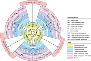
Recently, a system of taxonomy and classification of network topology and network morphology was introduced.Footnote 2[Reference Zok, Latture and Begley18] Its conceptual evolution can be represented by a “phylogenetic tree”, as depicted in Fig. 4. It begins with elementary cubic lattices, constructed by joining nearest-neighbor points of one of the three common cubic space lattices—simple cubic, body-centered cubic, and face-centered cubic—with struts. These lattices are denoted {SC}, {BCC}, and {FCC} [Fig. 2(e)]. In these cases, the lattice designations fully define both network topology and network morphology. An elementary non-cubic lattice is constructed by applying an affine transformation to an elementary cubic lattice such that the new nodal locations exhibit symmetry of a different space lattice but the connectivity of nodes remains fixed. Examples include face-centered tetragonal, {FCT}, formed by stretching an {FCC} lattice along one of the three principal directions, and rhombohedral, {R}, formed by stretching a {SC} lattice along the cube diagonal while maintaining constant strut lengths. When combined with the network topology, these transformations define the spatial relationships of nodes and hence the orientation and lengths of all struts, i.e., network morphology.
Phylogenetic tree showing the lattice classification system and its conceptual evolution, from elementary cubic lattices (at the center) to compound and non-cubic lattices of progressively increasing levels of complexity. Black arrowed lines show pathways through which lattices at lower levels are combined or modified to produce new lattice types. Lattices contained within domains bounded by dark gray lines have the same network topology but varying network morphology. Two of the complex lattices residing at the periphery are illustrated in Figs. 2(h) and 2(i).

A compound cubic lattice is constructed by combining two cubic lattices with identical unit cell edge lengths in a common Cartesian coordinate system. For example, combining a {SC} lattice with a {BCC} lattice yields a compound lattice of the form {BCC}|{SC} [Fig. 2(f)]. Variants on compound cubic lattices are obtained by scaling one of the parent elementary sub-lattices by an integer value of ≥2. This can produce, for example, a super compound lattice of the type {BCC}|{2SC} where the {BCC} sub-lattice has been scaled by a factor of 2; here two {SC} cells are needed over a linear distance equal to that of an individual {BCC} cell [Fig. 2(g)].
The process can be taken further to construct complex lattices [Figs. 2(h) and 2(i)].[Reference Zok, Latture and Begley18] These are made by either (i) assigning multiple nodes to each lattice point and then joining nearest-neighbor nodes with struts or (ii) assembling lattice subcells to form a supercell and tiling that supercell in space. For example, the diamond cubic lattice is constructed by assigning two nodes to each point of an FCC space lattice, at  $\left\lfloor {\matrix{ 0 & 0 & 0 \cr}} \right\rfloor$ and $\left\lfloor {\matrix{ {{1 / 4}} & {{1 / 4}} & {{1 / 4}} \cr}} \right\rfloor$ (the $\lfloor{} \rfloor$ brackets denoting nodal positions at a lattice point). The lattice is formed by joining nearest-neighbor nodes with struts. The resulting structure comprises tetrahedral subunits with four struts meeting at each node and each strut at 109.5° to each of the adjoining struts. The structure type is denoted as $\left\{ {{\rm FCC}\left\lfloor {\matrix{ 0 & 0 & 0 \cr}} \right\rfloor \left\lfloor {\matrix{ {{1 / 4}} & {{1 / 4}} & {{1 / 4}} \cr}} \right\rfloor} \right\}$.
The classification of network topology and network morphology, as described here, achieves two important goals: (i) it brings order into a field rife with disparate nomenclature and (ii) it provides a framework for systematic conceptual design of lattices with varying levels of complexity.
Structure–property relations: internal response to external stress
The internal response of lattice materials to external loads differs fundamentally from that of solid materials. When lattice materials are subjected to a macroscopically uniform strain, material elements within the lattice generally experience strains that differ appreciably from the applied strain and differ among the various strut populations. For example, when an {FCC} lattice material is loaded elastically in uniaxial compression along one of the principal material directions, 2/3 of the struts (those inclined at 45° to the loading direction) experience uniaxial compression along the strut axis and a strain equivalent to 1/3 of the applied macroscopic strain;[Reference Latture, Begley and Zok19,Reference Messner23] the remaining 1/3 (oriented perpendicular to the loading direction) experience uniaxial tension along the strut axis and a strain equivalent to −1/3 of the applied strain. When, instead, the same structure is loaded in uniaxial tension, 2/3 of the struts are in tension and 1/3 of the struts are in compression.
The preceding results have two important implications. First, the lateral (or Poisson) strain due to axial loading of a lattice material is not stress-free as it is in solid materials; these strains naturally have stresses associated with them. Second, regardless of whether a lattice material is loaded in tension or compression, some struts are always in tension while others are in compression. Consequently, compressive strength may be controlled by tensile strut rupture (if the material is relatively brittle), while tensile strength may be controlled by compressive strut buckling (if the material has a low modulus and a relatively high tensile ductility). In this context, the weaker of the two failure modes may dictate strength under both macroscopic tension and macroscopic compression. This type of behavior is not found in engineering solids.
Lattice defects and their role in properties
External surfaces
Relative to their effects in solids, external surfaces of lattice materials play an outsized role in lattice strength.[Reference Latture, Begley and Zok19,Reference Latture, Rodriguez, Holmes and Zok24] The effects arise from the reduced nodal connectivity of struts ending at these surfaces [Fig. 2(o)]. In the {FCC} lattice, for example, each strut within the bulk of the lattice has a nodal connectivity of 12 at each end; in contrast, when the lattice is present as a prismatic block with each face perpendicular to one of the [100] directions, nodal connectivities of struts located along the edges of the block (at intersections of pairs of external surfaces) are either 5 and 12 or 5 and 8 at the two ends, depending on strut orientation. Finite element simulations[Reference Latture, Begley and Zok19,Reference Messner23] and experimental strain measurements via digital image correlation[Reference Latture, Rodriguez, Holmes and Zok24] have shown that, when such a block is loaded in compression along the [100] direction, axial strains in struts oriented perpendicular to the loading direction and located at a block edge are 50% greater than those of equivalent struts in the bulk. Thus, when failure is controlled by tensile strut rupture, the strength of a lattice with external surfaces can only attain 2/3 of that expected of the bulk lattice.
The sensitivity of strut strains to external surfaces depends on network topology and network morphology in the following way. The compound cubic lattice  $60\% \,{\lcub {{\rm BCC}} \rcub } \vert 40\% \,\lcub {{\rm SC}} \rcub$ (percentages being adjusted by varying strut diameters) has been studied recently [Fig. 2(f)] because it exhibits isotropic elastic response with a stiffness equal to the theoretical upper bound for strut-based lattices.[Reference Latture, Begley and Zok19,Reference Latture, Begley and Zok25,Reference Gurtner and Durand26] (Its stiffness is 50% greater than that of the {FCC} lattice in the [100] direction.) When loaded elastically in compression in the [100] direction, the {SC} struts oriented perpendicular to the load direction experience uniaxial tension with a strain equivalent to −1/4 of the applied strain (lower in magnitude than the ratio of −1/3 in {FCC}, by 25%). When present at external surfaces, the same struts experience a strain of −0.29 of the applied strain: only about 16% greater than that in the lattice interior. Consequently, when failure is controlled by tensile strut rupture, the sensitivity of lattice strength to the presence of external surfaces is lower in the compound lattice than in the {FCC} lattice.
The degree to which external surfaces affect lattice strength depends also on the intrinsic failure properties of the constituent materials. Assuming that lattice failure occurs when the first tensile strut breaks, the predicted lattice strength, σ f, expressed in nondimensional form, is σ f/E oρ = (E/E oρ)(ɛ 1/kɛ a)ɛ f, where E and E o are the Young's moduli of the lattice and the constituent material, respectively, ρ is the relative density of the lattice, ɛ is the applied strain, ɛ a is the resulting axial strain in the tensile struts within the bulk of the lattice, and k is the maximum strain amplification in tensile struts at external surfaces.[Reference Latture, Begley and Zok19] For the {FCC} lattice, E/E oρ = 1/9 and ɛ 1/kɛ a = 2, and thus, the lattice strength is σ f/E oρ = 0.22ɛ f. For the compound lattice  $60\%\, {\lcub {{\rm BCC}} \rcub } \vert 40\%\, \lcub {{\rm SC}} \rcub$, E/E oρ = 1/6 and ɛ 1/kɛ a = 3.41, and the lattice strength is σ f/E oρ = 0.57ɛ f. Therefore, for fixed relative density and material failure strain, the strength of the compound lattice is predicted to be about 2.5 times that of the {FCC} lattice. In both cases, however, failure initiates at the external surfaces. When, instead, the tensile failure strain is high and failure is controlled by strut buckling, the {FCC} lattice is superior because of a higher buckle-initiation stress. Interestingly, unlike tensile strut rupture, buckling failure is essentially independent of the presence of free surfaces in well-designed lattices.
External surfaces in lattice materials are also manifested in unique ways in fracture toughness. In the presence of a through-crack in a block of lattice material, failure initiates near the juncture of the crack tip and an external surface; here the nodal connectivity is lowest. Surface-initiated fracture occurs regardless of the thickness of the block parallel to the crack front. It implies, most importantly, that the plane-stress fracture toughness is lower than the plane-strain fracture toughness (V. Deshpande, private communication): a result unlike that found in any other engineering material.
In light of the role of external surfaces of lattice materials in their mechanical properties, potential remediation strategies, based on new forms of surface engineering, are indicated. In traditional materials science, surface engineering encompasses processes such as case hardening by nitridation or carburization, anodizing by electrolytic passivation, and coating by chemical or physical vapor routes. But the nature of surface engineering in lattice materials would take a very different form. Here, the goal would be to alter the load transfer characteristics among struts at external surfaces. This could be achieved by either (i) selective addition of near-surface struts that would not be present in the bulk or (ii) cshanges in strut cross-sections (or other morphological characteristics) in near-surface regions [Fig. 2(o)]. This topic remains unexplored.
Strut defects
Structural defects in lattice materials are distinctly different from those found in solid engineering materials. Several defect types (apart from external surfaces) have been identified and studied. Missing or defective struts—caused by incomplete fusion, curing, or densification during fabrication—are obvious candidates. Such defects will generally concentrate strains in surrounding struts and possibly trigger premature failure [Fig. 2(m)]. But, in some lattice materials, such as the {FCC}, strain concentrations around missing struts are less than those inherent to external surfaces.[Reference Latture, Begley and Zok19] In these cases, lattice strength is virtually independent of an individual missing strut, even when that missing strut is located at the external surface; the external surface itself dominates. Effects of missing struts in the {FCC} lattice are only manifested when the number of missing struts becomes a significant fraction of the total number of struts.[Reference Wallach and Gibson27] In other lattice types, such as the compound  $60\%\, {\lcub {{\rm BCC}} \rcub } \vert 40\%\, \lcub {{\rm SC}} \rcub$, missing {SC} struts aligned with the loading direction concentrate strain, by about 20% more than that associated with the external surfaces.[Reference Latture, Begley and Zok19] When located at the surfaces, such defects can reduce the lattice strength, beyond that due to the surfaces alone. These scenarios demonstrate that the sensitivity of lattice strength to missing struts is affected by lattice topology: analogous, for example, to the role of crystal structure in the varying sensitivities of yield and creep strengths to crystal defects in solid engineering materials.
Nodes
Nodes at which struts intersect represent an important lattice feature [Fig. 2(n)].[Reference Latture, Rodriguez, Holmes and Zok24,Reference Hammetter, Rinaldi and Zok28,Reference Portela, Greer and Kochmann29] They are, in a sense, loosely analogous to grain boundaries in polycrystalline materials: both transmit loads between adjoining regions and both may serve as potential sites of failure initiation. In this context, nodes in lattice materials are both essential structural features and potential defects. Nodes are particularly vulnerable to failure because of overlapping strut volume at the nodes, the local load bearing area is reduced, and hence, the local stress is elevated relative to that in regions distal from the nodes. Moreover, when sharp changes in cross section are present at strut intersections, local stresses may be elevated further. Thus, if no adjustment is made to local geometry to compensate for these effects, yielding or fracture is likely to initiate within the node regions, not within the struts themselves.[Reference Latture, Rodriguez, Holmes and Zok24,Reference Hammetter, Rinaldi and Zok28] The design of nodes to effectively transmit loads between adjoining struts while minimizing stress concentrations remains a largely unexplored area of research.
Other lattice defects
Other lattice defects, specific to certain fabrication routes, have also been identified. Examples include: (i) strut waviness, a feature inherent to woven metal lattices;[Reference Kang22,Reference Queheillalt, Deshpande and Wadley30] (ii) variations in strut cross-section, either stochastic[Reference Salari-Sharif, Godfrey, Tootkaboni and Valdevit31] or systematic, the latter obtained in polymer lattices made by self-propagating photocuring;[Reference Rinaldi, Bernal-Ostos, Hammetter, Jacobsen and Zok32,Reference Rinaldi, Hammetter and Zok33] and (iii) roughness on strut surfaces, invariably found in metallic lattices fabricated by selective electron beam melting[Reference Campoli, Borleffs, Yavari, Wauthle, Weinans and Zadpoor34,Reference Hernandez-Nava, Smith, Derguti, Tammas-Williams, Leonard, Withers, Todd and Goodall35] or selective laser melting.[Reference Liu, Kamm, García-Moreno, Banhart and Pasini36]
Lattice material design
Optimization of lattice properties requires concurrent selection of topology, morphology, and constituent material. Structure–property relations represent the key enabling links. The following example illustrates how these relations can be used in the design of lattice materials.
The compressive strength of a lattice material is generally governed by one of three failure modes: (i) buckling of struts loaded in compression, (ii) tensile fracture of struts load in tension, or (iii) yielding of the most heavily strained struts (assuming that the node geometry has been designed to ensure that the node remains elastic when the struts yield). A rudimentary analysis can be performed for cases in which the yield strain exceeds the tensile fracture strain. For the {FCC} lattice, strut buckling occurs at a critical macroscopic stress, expressed in nondimensional form: σ f/E oρ 2 = 0.056.[Reference Latture, Begley and Zok19] The corresponding macroscopic stress needed to break the most heavily strained tensile strut (expressed in the same nondimensional form) is σ f/E oρ 2 = 0.22ɛ f/ρ.[Reference Latture, Begley and Zok19] The two strengths are equal to one another when ɛ f/ρ = 0.25. One implication is that the full strength potential of the {FCC} lattice (controlled by buckling) is only attained when the material failure strain satisfies the condition ɛ f ≥ 0.25ρ. This condition is conceivably attainable with a hard, high-ductility plastic; a failure strain of ɛ f = 0.05 would satisfy this condition for relative densities up to ρ = 0.2. In contrast, if the lattice were made of a plastic with ɛ f = 0.01, the condition would only be satisfied for relative densities up to ρ = 0.04. This rudimentary case study illustrates how topology, morphology (especially relative density), and material can be selected concurrently in order to attain lattice materials with optimal properties.
Outlook
The present article has highlighted the unique nature of structure of low-order periodic lattice materials and a unifying taxonomy that allows systematic conceptual design of lattices with varying levels of complexity. It has also illustrated structure–property relations as they pertain to lattice strength and how these relations could be integrated into the processing–structure–properties paradigm of traditional materials science. While the fundamental understanding of lattice materials has grown appreciably in the past decade, the field will undoubtedly grow even more rapidly in the coming decade, due in no small part to the explosive growth in modern additive manufacturing technologies coupled with the vast and varied application potential of lattice materials.
In addition to the low-order systems described here, a number of concepts in high-order structural lattices—ones that were practically inconceivable because of manufacturing limitations a decade ago—are emerging. Hierarchical lattices are one example [Fig. 2(k)].[Reference Wu, Vaziri, Asl, Ghosh, Gao, Wei, Ma, Xiong and Wu37,Reference Doty, Kolodziejska and Jacobsen38] Most reported studies have been theoretical or computational in nature, with only few demonstrations of fabricated structures.[Reference Zheng, Smith, Jackson, Moran, Cui, Chen, Ye, Fang, Rodriguez, Weisgraber and Spadaccini39] Moreover, studies on structural hierarchical lattices have focused to a large extent on stiffness and strength of lattice topologies that are inherently compliant and weak (e.g., 2D hexagonal lattices).[Reference Ajdari, Jahromi, Papadopoulos, Nayeb-Hashemi and Vaziri40–Reference Chen, Jia and Wang45] These lattices are bend-dominated and therefore exhibit properties that are inferior to those of triangulated (stretch-dominated) lattices. Although stiffness and strength of bend-dominated lattices can be readily improved through hierarchical design, there is little compelling evidence to support the notion that hierarchical designs are superior in stiffness or strength to well-designed, single-scale, stretch-dominated lattices.[Reference Banerjee46] On the contrary, one study has shown that 3D lattice materials based on the {FCC} or the {BCC}|{SC} lattices are, in fact, degraded by hierarchical design.[Reference Vigliotti and Pasini47] A further issue that has yet to be addressed is the increase in node density that accompanies hierarchical design. It is likely that some of the benefits from hierarchical designs (if and when it can be realized) will be offset by the increased proportion of material that will need to be allocated to the node regions to ensure robust node properties.
Other concepts, based on graded lattices [Fig. 2(j)], may have utility in cases where the desired mechanical response involves a progressive change in crushing resistance.[Reference Wang, Zheng and Yu48–Reference Kiernan, Cui and Gilchrist50] Conceptually, grading can be accomplished in one of three ways: (i) by spatially varying material composition or material state (e.g., degree of polymer curing or cross-linking), (ii) by progressively varying strut angles, or (iii) by progressively varying strut cross-sections.
High-order lattices based on poly-topological designs can also be envisioned [Fig. 2(m)]. These could be designed in a manner analogous to conventional engineered composites. That is, domains in which the response is stiff and strong might be combined judiciously with surrounding domains in which the response is more compliant, potentially exploiting the attractive attributes of the two respective lattice types. These lattices would introduce new defects: domain boundaries between regions with differing lattice orientation or lattice topology, analogous to grain or interphase boundaries in solid polycrystalline materials.
Going beyond lattice materials, the framework described here could be extended to include other lightweight materials with periodic arrangements of constituent elements. Notable among these are cellular materials with triply-periodic minimal-surface (TPMS) architectures. Although the nature of TPMS geometries and specific prototypical architectures are well established, investigations into their practical use as engineered materials are just now emerging. One particularly promising application is in orthopedic implants where the combination of structural stiffness and strength, high permeability and surface area, and near-zero average curvature of TPMS structures allows designs that closely mimic bone.[Reference Bobbert, Lietaert, Eftekhari, Pouran, Ahmadi, Weinans and Zadpoor51,Reference Yan, Hao, Hussein and Young52]
As yet, the science and engineering communities collectively have tapped into only a small fraction of the full potential of lattice materials. As with the successful evolution of other classes of engineering materials, the study of lattice materials within an expanded materials science framework should significantly accelerate both the material development process and the adoption of these materials in engineering applications.
Acknowledgments
This article is dedicated to Professor J. David Embury in honor of his 80th birthday and in recognition of his immense contributions to materials science during his illustrious career. Indeed, a recent honorary Embury symposium on the future of materials science provided the impetus for preparation of this article.
This work was supported by the Institute for Collaborative Biotechnologies through Task 51: Structural Materials with Enhanced Resilience and Response Properties, Award Number W911NF-09-D-0001-0051. The content of the information does not necessarily reflect the position or the policy of the Government, and no official endorsement should be inferred.


 Open access