


Introduction
Weed management remains one of the major challenges in modern agriculture, profoundly influencing both crop yield and quality. Weeds are generally defined as plants that grow where they are not desired and compete with crops for essential resources, thereby constraining sustainable agricultural development (Kumar et al. Reference Kumar, Kumari and Rana2024). Globally, weeds are recognized as a dominant factor limiting crop productivity, accounting for an estimated 37% of total yield losses, compared with 29% and 22% caused by insect pests and plant diseases, respectively (Demjanová et al. Reference Demjanová, Macák, Dalovic, Majernik and Tyr2009). In this context, exploring diversified cropping systems and developing site-specific or variable-rate spraying technologies have become crucial strategies to enhance crop productivity and promote efficient, sustainable weed control (Wang et al. Reference Wang, Li and Jia2025).
The soybean [Glycine max (L.) Merr.]–maize (Zea mays L.) strip intercropping system has evolved from traditional intercropping and relay-cropping practices (Monteiro and Santos Reference Monteiro and Santos2022). During the growing period, the temporal and spatial complementarity between maize and soybean enables more efficient utilization of light, water, and nutrients, thereby improving overall crop yield (Chen et al. Reference Chen, Jiang, Zhang, Zhang, Jiang and Gao2025). Weeds hinder the growth of crops by competing with the plants for water, nutrients, and sunlight, which results in large losses in crop production (Monteiro and Santos Reference Monteiro and Santos2022). Therefore, in the soybean–maize intercropping system, the implementation of variable-rate spraying technology is essential for improving crop yield. Traditional spraying practices typically apply a uniform pesticide rate across the entire operation area in a single continuous pass. However, this approach does not take into account the spatial variability and distribution differences of weeds, pests, and diseases within the field. As a result, the amount of active ingredient applied is often insufficient in areas with severe infestations, while excessive in areas with light or no infestations (He Reference He2020). Under such traditional spraying practices, pesticide application can easily lead to serious environmental contamination and considerable chemical waste (He Reference He2018). Variable-rate spraying technology, by contrast, can precisely adjust the herbicide application rate according to weed and pest distribution, vehicle speed, and crop growth status, effectively addressing the shortcomings of traditional spraying methods (Wen et al. Reference Wen, Zhang, Deng, Lan and Yin2018).
Variable-rate spraying technology can generally be classified into three main types: pressure-regulated control, liquid concentration-regulated control, and pulse-width modulation (PWM)-based control (Abbas and Han Reference Abbas and Han2024; C Zhang et al. Reference Zhang, Zhai, Zhang, Zhang, Zou and Zhao2024). Pressure-based variable-rate spraying achieves variable application by altering the internal pipeline pressure, thereby changing the spray volume. Zhang et al. (Reference Zhang, Ma and Chen2025) developed a pressure-based variable-rate spraying system in which spray pressure was regulated by adjusting the pesticide pump voltage; their study demonstrated that the coefficient of variation in spray distribution reached 16.93%, which was significantly lower than the 23.76% obtained with the single regulation method. However, pressure-regulated systems frequently exhibit unstable spray performance and limited precision. In contrast, liquid concentration-regulated systems typically offer superior spray quality and higher control accuracy. Liu et al. (Reference Liu, Xu and Hong2009) designed a real-time mixing variable-rate spraying system that adjusted pesticide concentration according to crop requirements using a chemical mixer; tests indicated that liquid uniformity was significantly improved, with a maximum average relative error of ±3%. Jiang et al. (Reference Jiang, Zhou and Li2015) investigated a PWM-based variable-rate spraying system, testing individual nozzles at different duty cycles and frequencies. Their findings indicated that once the duty cycle reached a threshold sufficient to stabilize flow, further increases in duty cycle led to improved spray uniformity both along the boom and in the nozzle’s travel direction.
With the advancement of information technology (Liu et al. Reference Liu, Abbas and Noor2021; R Wang et al. Reference Wang, Li, Men, Gao and Xu2022; Zheng et al. Reference Zheng, Zhao, Han, He, Zhai and Zhao2023), novel algorithms have been increasingly adopted for variable-rate spraying control (He et al. Reference He, Ding, Ji, Jin, Feng and Hao2024). Sheng et al. (Reference Sheng, Zhang, Deng, Lan, Yin and Shan2018) developed a UAV-based variable-rate spraying system that interpreted prescription maps in real time to obtain target values; a proportional-integral-derivative (PID) control algorithm then adjusted the duty cycle accordingly to regulate flow rate. Experimental evaluation demonstrated that the deviation between the theoretical and actual flow rates did not exceed 2.16%, reflecting precise and stable spray control performance. Hao et al. (Reference Hao, Ai and Yuan2024) designed a pesticide application machine for a maize–peanut (Arachis hypogaea L.) strip intercropping system based on an incremental PID algorithm, achieving variable-rate application by adjusting the opening of a proportional control valve in real time. Field trials indicated that the difference between the applied dosage and the theoretical value was 2.1%. Zhao et al. (Reference Zhao, Hu and Liu2024) introduced the artificial bee swarm algorithm into variable-rate spraying to optimize the PID controller parameters—namely, the proportional gain ( $K_p$
), integral gain (
$K_p$
), integral gain ( $K_i$
), and derivative gain (
$K_i$
), and derivative gain ( $K_d$
)—for improved control performance. Experimental evaluation demonstrated substantial improvements in suppressing overshoot and enhancing control accuracy, indicating the effectiveness of the proposed spraying control strategy.
$K_d$
)—for improved control performance. Experimental evaluation demonstrated substantial improvements in suppressing overshoot and enhancing control accuracy, indicating the effectiveness of the proposed spraying control strategy.
In summary, conventional PID parameter-tuning methods still largely rely on empirical approaches, which are not only time-consuming not easily adaptable to complex dynamic systems (Song et al. Reference Song, Li, Chen, Xia, Zhang and Tang2022). Fuzzy PID controllers can adjust PID parameters online according to system error and its rate of change, thereby enhancing control performance, robustness, and system stability under varying operating conditions (Luo et al. Reference Luo, Deng, Huo, Zhang, Ye, Lei and Zhang2024). However, determining the optimal parameters for fuzzy PID controllers remains a challenging task. To address this issue, this study employs an improved beetle antennae search (IBAS) algorithm to identify the optimal fuzzy PID parameters. BAS is a nature-inspired optimization method that simulates beetle foraging behavior, updating candidate solutions based on the differences in objective function values detected at the two antennae. Although conventional BAS is simple, computationally efficient, and possesses strong global search capability, it is prone to premature convergence and sensitive to step size, and it exhibits limited adaptability to dynamic or time-varying systems (H Ding et al. Reference Ding, Yuan and Deng2025). In this study, the IBAS algorithm is applied to optimize fuzzy PID parameters, thereby enhancing both the control accuracy and robustness of the variable-rate spraying system.
Materials and Methods
Experimental Conditions and Equipment
To evaluate the spraying control performance of the IBAS–fuzzy PID algorithm, field experiments were conducted from July 4 to July 9, 2025, at the core demonstration site for soybean–maize strip intercropping in Xuzhou, China. The spraying target was maize. During the trial period, weather conditions were clear with a wind speed of 1.5 m s−1. The maize–soybean strip intercropping sprayer is shown in Figure 1.
(A) Soybean–maize strip intercropping sprayer; and (B) schematic diagram of the variable-rate spraying system.

System Composition and Design
System Composition
The structure and components of the variable-rate spraying system for the maize–soybean strip intercropping sprayer are illustrated in Figure 2. Due to the differing pesticide tolerances between maize and soybean, two independent pipeline systems were designed to apply pesticides separately. To prevent cross-contamination of pesticides, the system employs anti-drift nozzles (Lechler GmbH, Remshalden, Germany), and soybean nozzles are equipped with protective covers. During operation, a peristaltic pump (Kamoer, Shanghai, China) delivers pesticide from the chemical tank through pipelines to the jet mixers (Huamei, Weifang, China). Simultaneously, a water pump supplies water from the water tank to the jet mixers, where it mixes with pesticide, resulting in a uniformly blended spray solution. The nozzle spacing is 40 cm for soybean and 36 cm for maize. The mixed solution then flows through pressure sensors (SGN, Jiangsu, China), flow sensors (Xinzun Technology, Shandong, China), and high-speed solenoid valves (AirTAC, Taiwan) before being supplied to the anti-drift nozzles. Every three nozzles constitute a group for pesticide application. The flow and pressure sensors transmit signals to the variable-rate spraying controller to monitor real-time system flow and pressure. High-speed solenoid valves serve as the primary actuators in the variable-rate spraying system, controlling the opening and closing of each individual nozzle. The controller receives pesticide application commands by analyzing prescription maps and adjusts the PWM duty cycle of the high-speed solenoid valves accordingly, thereby modulating nozzle flow to achieve variable-rate spraying.
Structure and components of the soybean–maize variable-rate spraying system: (1) water tank (1,000 L); (2) maize pesticide tank (7 L); (3) peristaltic pump; (4) jet mixer; (5) chemical mixer; (6) pressure sensor; (7) flow sensor; (8) anti-drift nozzle; (9) high-speed solenoid valve; (10) check valve; (11) pressure-regulating valve; (12) water pump; (13) protective cover; (14) soybean pesticide tank (7 L); (15) variable-rate controller; (16) speed sensor.

Hardware Design
In the variable-rate spraying system, an STM32F103ZET6 72MHz (STMicroelectronics, Geneva, Switzerland) a microcontroller was employed as the controller. Signals from the speed, pressure, and flow sensors were acquired and processed in real time. The PWM duty cycle of the solenoid valve was adjusted according to a pre-generated prescription map to achieve dynamic regulation of the spray rate. The prescription map was developed based on the analysis of the leaf area index (LAI) and plant height of soybean–maize, enabling variable-rate spraying control to be implemented according to crop growth characteristics. The sensors used include a BRT38-V5M4086-RT1 (BRITER, Shenzhen, China) speed encoder, a QDW90A-VD pressure transmitter with a measurement range of 0 to 1 MPa, and an OF06ZAT turbine flow meter with a range of 5 to 200 L min−1. A 12-V automotive power supply (Chaowei, Zhejiang, China) was used to provide power to the sensors. The solenoid valves operated at a rated voltage of 12 V, whereas the output voltage of the microcontroller pins was 3.3 V, insufficient for direct actuation. To achieve rapid switching, the valves were controlled via a metal-oxide semiconductor transistor as an electronic switch, driven by the PWM signal from the microcontroller. When the output pin voltage was 0 V, the transistor remained off; when the voltage was 3.3 V, the transistor was turned on. Through this configuration, the 12-V power supply could be switched on and off effectively, allowing the voltage across the solenoid valves to alternate between 0 and 12 V and enabling fast and stable opening and closing of the valves. To protect the transistor from potential voltage spikes generated when the solenoid valves close, a diode protection circuit was installed. Figure 3 illustrates the hardware structure of the variable-rate spraying system, along with the corresponding calculation formulae for each parameter.
Composition of variable-rate spraying system hardware structure. RX, receive; TX, transmit; ADC, analog to digital converter; I/O, input/output; IC, input capture.

Speed Parameter Measurement
The speed encoder is connected to the rear wheel axle of the tractor via a coupling, as illustrated in Figure 4. The speed encoder outputs an analog voltage signal ranging from 0 to 5 V to the STM32 microcontroller, corresponding to a rotational speed range of 0 to 3,000 rpm. The analog voltage is linearly related to the rotational speed, allowing the current travel speed to be determined based on the measured voltage. Because the STM32 microcontroller can only accept input voltages between 0 and 3.3 V, an AD conversion voltage module is used to linearly convert the 0- to 5-V signal to the 0- to 3.3-V range, ensuring compatibility with the STM32’s voltage input limits. Vehicle speed is calculated by the following formula:
 $${{v}} = {{{{360}}\pi {{rA}}} \over {{{4}},{{095}}}}$$
where v is vehicle speed (km h−1), r is the wheel’s radius (m), and A is the STM32 ADC sampling value ranging from 0 to 4,095.
Schematic diagram of the speed encoder.

Pressure Parameter Measurement
The pressure sensor is installed in the pipeline to monitor whether the internal pressure remains within a safe range, thereby preventing occurrences such as pipeline rupture, pressure release, or sudden pressure fluctuations. The pressure sensor is shown in Figure 5. The pressure sensor used in this study outputs an analog voltage of 0 to 5 V, similar to the speed sensor, and is processed using the same method. The pressure is calculated using the following formula:
 $$P = (P_{\rm max} - P_{\rm min}) \times {A \over 4\,095}$$
Schematic diagram of the pressure sensor.

where ${{P}}$
represents the measured pressure (MPa);
${{P}}$
represents the measured pressure (MPa); ${{{P}}_{{{\rm max}}}}$
and
${{{P}}_{{{\rm max}}}}$
and ${{{P}}_{{{\rm min}}}}$
denote the upper and lower measurement limits of the pressure sensor, which are set to 1 MPa and 0 MPa, respectively; and
${{{P}}_{{{\rm min}}}}$
denote the upper and lower measurement limits of the pressure sensor, which are set to 1 MPa and 0 MPa, respectively; and ${{A}}$
is the 12-bit ADC value sampled by the STM32 microcontroller, ranging from 0 to 4,095.
${{A}}$
is the 12-bit ADC value sampled by the STM32 microcontroller, ranging from 0 to 4,095.
Flow Parameter Measurement
The flow sensor is installed in front of the nozzle and behind the solenoid valve. The pressure regulator stabilizes the internal pipeline pressure to prevent the impact of transient pressure spikes caused by the rapid opening and closing of the solenoid valve. The installation positions are shown in Figure 6. The liquid passing through the sensor is sprayed through the nozzle, so the measured flow rate corresponds to the actual flow rate. A Hall element is a semiconductor device that is sensitive to magnetic fields. In the flow sensor, the turbine is driven to rotate by the fluid flow, causing the magnets mounted on the turbine to produce variations in the magnetic field. These variations are detected by the Hall element and converted into voltage pulse signals. The pulse frequency is proportional to the flow rate, which allows the actual flow rate to be determined. The flow rate is calculated by the following formula:
 $${{Q}} = {{{{N}}\; \times \;{{60}}} \over {{K}}}$$
Schematic of the flow sensor installation.

where ${{Q}}$
is the flow rate (L min−1), N is the number of pulses counted within 1 s, and K is the flow coefficient (540 pulses L−1).
${{Q}}$
is the flow rate (L min−1), N is the number of pulses counted within 1 s, and K is the flow coefficient (540 pulses L−1).
IBAS-based Search Algorithm
BAS Algorithm
The beetle antennae search (BAS) algorithm (Jiang et al. Reference Jiang, Zhou and Li2015) is a heuristic optimization algorithm inspired by the foraging behavior of beetles in nature. Beetles use their antennae to sense odors: if the left antenna detects a stronger scent than the right, the beetle moves left, and vice versa. This process iterates until the beetle finds food. Compared with other optimization algorithms, BAS is simple and efficient, requiring only one beetle (individual) for searching, making it more lightweight than particle swarm optimization or genetic algorithms. The optimization procedure consists of the following three steps:
-
Step 1: Randomly generate an n-dimensional vector $X = (X_1, X_2, X_3, \ldots, X_n)$
, and normalize it to a unit vector:([4])
$${{c}} = {{{{\rm rand}}({{n}},\;{{1}})} \over ||{{{\rm rand}}({{n}},\;{{1}}){{||}}}}$$
$X = (X_1, X_2, X_3, \ldots, X_n)$
, and normalize it to a unit vector:([4])
$${{c}} = {{{{\rm rand}}({{n}},\;{{1}})} \over ||{{{\rm rand}}({{n}},\;{{1}}){{||}}}}$$


where ${{rand(n,\;1)}}$
represents a random function generating an
${{rand(n,\;1)}}$
represents a random function generating an ${{n\; \times \;1}}$
vector, and
${{n\; \times \;1}}$
vector, and ${{c}}$
is a unit vector with a magnitude of 1.
${{c}}$
is a unit vector with a magnitude of 1.
-
Step 2: Define
${{{X}}_{{l}}}$
and
${{{X}}_{{r}}}$
as the left and right antenna coordinates, respectively,
${{A}}$
as the centroid coordinate, and
${{{d}}_{{0}}}$
as the distance between the two antennae:([5])
$$\;\left\{ {{{{{{X}}_{{l}}} = {{X}}\;{{ + }}\;{{{d}}_{{0}}}{{^*c}}} \over {{{{X}}_{{r}}} = {{X}} - {{{d}}_{{0}}}{{^*c}}}}} \right.\;$$
-
Step 3: Determine the moving direction and find the next position. For the fitness function
$f$
, the responses at the left and right antenna positions are computed as
${f_{left}}$
=
$f{\hbox{(}\rm X_l\hbox{)}}$
and
${f_{right}}$
=
$f\bigl(\rm X_{r}\bigr)$
. The beetle advances by a distance of step in the direction of the antenna corresponding to the higher fitness value; specifically, if
${f_{\rm left}}\;$
>
$\;{f_{\rm right}}$
, it moves toward the left antenna, otherwise, it moves toward the right antenna:([6])
$$\left\{ {\matrix{ {{X_{t + 1\;}} = \;{X_t}\; + \;{\rm step}^*{\rm nor}\left( {{X_l}\; - \;{X_r}} \right),\;\;{f_{\rm left}}\; \gt \;{f_{\rm right}}} \cr {{X_{t + 1}}\; = \;{X_t}\; - \;{\rm step}^*{\rm nor}\left( {{X_l}\; - \;{X_r}} \right),\;\;{f_{\rm left}}\; \lt \;{f_{\rm right}}} \cr } } \right.$$


where step denotes the search step size; t is the iteration number; $f{\it\hbox(} {{X_l}} {\it\hbox)}$
and
$f{\it\hbox(} {{X_l}} {\it\hbox)}$
and $f{\it\hbox ( }{{X_r}} {\it\hbox )}$
represent the odor intensities sensed by the beetle’s left and right antennae, corresponding to the fitness function values; and
$f{\it\hbox ( }{{X_r}} {\it\hbox )}$
represent the odor intensities sensed by the beetle’s left and right antennae, corresponding to the fitness function values; and ${{nor}}\left( \cdot \right)$
denotes the normalization function.
${{nor}}\left( \cdot \right)$
denotes the normalization function.
IBAS Algorithm
The traditional BAS algorithm searches by randomly generating direction vectors. However, an unfavorable initial position may cause premature convergence to a local optimum, limiting the global search capability. While BAS performs well in low-dimensional problems, its accuracy and convergence speed decline in high-dimensional scenarios, increasing the likelihood of being trapped in local optima. To address these issues, this study introduces a chaotic mapping strategy to optimize the BAS algorithm.
The introduction of chaotic perturbation allows the algorithm to escape local optima by driving the individual through nonlinear disturbances generated by chaotic sequences when stagnation occurs. Due to the excellent ergodicity, randomness, and sensitivity to initial conditions of chaotic sequences, the search process gains increased diversity and dynamics, enhancing the algorithm’s global optimization capability and convergence speed. Common chaotic mapping methods (Varol and Alatas Reference Varol and Alatas2020) include logistic map, tent map, Chebyshev map, and iterative map. This study adopts the logistic chaotic map due to its superior ergodicity, randomness, and sensitivity to initial values (C Zhang et al. Reference Zhang, Zhai, Zhang, Zhang, Zou and Zhao2024). The calculation formula of the logistic chaotic map is as follows:
 $${{{x}}_{{{n + 1}}}}{{\;}}{{ = \;r^*}}{{{x}}_{{n}}}{{^*(1\; - \;}}{{{x}}_{{n}}}{{)}}$$
where ${{r}}$
is the control parameter ranging in (0, 4); the degree of chaos increases with
${{r}}$
is the control parameter ranging in (0, 4); the degree of chaos increases with ${{r}}$
, and the system reaches full chaos when
${{r}}$
, and the system reaches full chaos when ${{r\;}}$
= 4, which is the value used in this study;
${{r\;}}$
= 4, which is the value used in this study; ${{{x}}_{{n}}}$
denotes the state value at the
${{{x}}_{{n}}}$
denotes the state value at the ${{n}}$
th iteration, and
${{n}}$
th iteration, and ${{{x}}_{{{n + 1}}}}$
is the next iteration value calculated based on the current state.
${{{x}}_{{{n + 1}}}}$
is the next iteration value calculated based on the current state.
In the BAS algorithm, the search direction is typically generated by normalizing a random vector. Although this method is simple and efficient, it does not utilize historical optimal solutions; thus, the search direction relies entirely on random perturbations, resulting in a stochastic search path. To address this, the present study introduces a guided direction perturbation mechanism, which preserves the exploratory randomness while incorporating the historical best solution to improve search efficiency. The calculation formulae are as follows:
 $${{b}} = ({{1}} - \alpha ){{^*}}{{{c}} \over {{{||c||}}}}{{ + }}\alpha {{^*}}{{{{{x}}_{{{\rm best}}}}{{ - }}\;{{{x}}_{{{\rm current}}}}} \over {{{||}}{{{x}}_{{{\rm best}}}} - {{{x}}_{{{\rm current}}}}{{||}}}}$$
 $${{b}} = {{{b}} \over {{{||b||}}}}$$
where ${{c}}$
is a random vector sampled from a uniform distribution over (−1, 1);
${{c}}$
is a random vector sampled from a uniform distribution over (−1, 1); ${{{x}}_{{{\rm best}}}}$
is the current global best solution;
${{{x}}_{{{\rm best}}}}$
is the current global best solution; ${{{x}}_{{{\rm current}}}}$
is the current position of the search individual; and
${{{x}}_{{{\rm current}}}}$
is the current position of the search individual; and ${{\alpha }}$
is the guidance factor balancing the weights of the guided and random terms, with
${{\alpha }}$
is the guidance factor balancing the weights of the guided and random terms, with ${{\alpha \;}}$
= 0.2 in this study.
${{\alpha \;}}$
= 0.2 in this study.
Finally, the vector ${{b}}$
is normalized to ensure the perturbation direction is a unit vector, facilitating decoupling from the step size.
${{b}}$
is normalized to ensure the perturbation direction is a unit vector, facilitating decoupling from the step size.
In the basic BAS algorithm, the step size remains fixed throughout the search process. A small step size in the early stage slows down the search speed, while a large step size in the later stage may cause oscillations near the optimal solution or lead to entrapment in local optima. To address this, the present study introduces a dynamic decaying step size factor. A larger step size is employed during the early phase of the search to broadly explore potential global optima and accelerate the global search, whereas a smaller step size is used near the optimum in the later phase to enhance local search precision and improve result stability. The formulae are as follows:
 $${\rm{ste}}{{\rm{p}}_t} = {\rm{ste}}{{\rm{p}}_0}^{*}r$$
 $${{r = }}\,\,{{{r}}^{{{t - 1}}}}$$
where ${\rm{ste}}{{\rm{p}}_0}$
is the initial step size controlling the exploration scale in the early phase, set to 0.5;
${\rm{ste}}{{\rm{p}}_0}$
is the initial step size controlling the exploration scale in the early phase, set to 0.5; ${{r}}$
is the step decay factor controlling the convergence rate, set to 0.95; and
${{r}}$
is the step decay factor controlling the convergence rate, set to 0.95; and ${{t}}$
is the current iteration number.
${{t}}$
is the current iteration number.
As the iteration count increases, the step size decreases exponentially, satisfying the requirement of a large step size during early search and a smaller step size during later search.
In this study, there are five parameters to be optimized. The basic BAS algorithm, with a dimensionality higher than five, suffers from reduced search accuracy and slower convergence speed, making it more prone to becoming trapped in local optima during iterations. To address these issues, the BAS algorithm is enhanced by incorporating the simulated annealing (SA) algorithm, thereby improving the algorithm’s accuracy (X Ding et al. Reference Ding, Yuan and Deng2025). The SA algorithm introduces stochastic elements into the search process. It accepts inferior solutions with a certain probability, increasing the likelihood of escaping local optima and achieving a global optimum. Here, ${{p}}$
denotes the probability of accepting a worse solution. The formulae are as follows:
${{p}}$
denotes the probability of accepting a worse solution. The formulae are as follows:
 $$p{\rm{\; = }}\,\left\{ {{\rm{}}\matrix{{\!\!\!\!\!\!\!\!\!\!\!\!\!\!\!\!\!\!\!\!\!\!1\!,\;} & {{f_{{\rm{new}}}} \lt {f_{{\rm{current}}}}} \cr {exp\left( { - {{{f_{{\rm{new}}}}{\rm{\;}} - {f_{{\rm{current}}}}} \over T}} \right),} & {{f_{{\rm{new}}}} \ge \;{f_{{\rm{current}}}}} \cr } } \right.$$
 $${{T = }}\,{{{T}}_{{0}}}{{^*}}{{{\rm{\beta }}}^{{t}}}$$
where ${{\;\;}}{{{f}}_{{{\rm current}}}}$
is the fitness value at the current position,
${{\;\;}}{{{f}}_{{{\rm current}}}}$
is the fitness value at the current position, ${{{f}}_{{{\rm new}}}}$
is the fitness value at the candidate updated position,
${{{f}}_{{{\rm new}}}}$
is the fitness value at the candidate updated position, ${{T}}$
is the current temperature,
${{T}}$
is the current temperature, ${{{T}}_{{0}}}$
is the initial temperature,
${{{T}}_{{0}}}$
is the initial temperature, ${{\rm exp}}\left( \cdot \right)$
denotes the natural exponential function,
${{\rm exp}}\left( \cdot \right)$
denotes the natural exponential function, ${\rm{\beta }}$
is the temperature decay coefficient, and
${\rm{\beta }}$
is the temperature decay coefficient, and $t$
is the current iteration number. As the iteration proceeds, the temperature gradually decreases, reducing the probability of accepting worse solutions.
$t$
is the current iteration number. As the iteration proceeds, the temperature gradually decreases, reducing the probability of accepting worse solutions.
IBAS-optimized Fuzzy PID Control Algorithm
PID Control
The PID controller is a linear feedback controller widely used in various engineering fields due to its high control accuracy (Nan et al. Reference Nan, Zhang, Zheng and Yang2023). Its fundamental principle is to continuously adjust the controlled object based on the error $e(\rm t)$
between the system’s target value
$e(\rm t)$
between the system’s target value $r(\rm t)$
and the feedback output
$r(\rm t)$
and the feedback output $y(\rm t)$
, so that the output approaches the target value, ultimately driving the error toward zero. The error is defined as follows:
$y(\rm t)$
, so that the output approaches the target value, ultimately driving the error toward zero. The error is defined as follows:
 $$e(\rm t) = r(\rm t) - y(\rm t)$$
The mathematical model of the PID controller is:
 $$u(\rm t) = K_{p}e(\rm t) + K_{i}\int_0^t e(\rm t)\,dt + K_{d}{{de(\rm t)}\over{dt}}$$
where ${{u(t)}}$
is the controller output,
${{u(t)}}$
is the controller output, ${K_p}$
is the proportional gain,
${K_p}$
is the proportional gain, ${K_i}$
is the integral gain, and
${K_i}$
is the integral gain, and ${K_d}$
is the derivative gain.
${K_d}$
is the derivative gain.
The classical PID controller is designed for linear time-invariant systems and exhibits poor control performance for nonlinear or time-varying systems, because its three parameters remain fixed and cannot self-adjust based on system states. To improve the control accuracy and response speed of the soybean–maize variable-rate spraying system, a fuzzy PID controller is introduced in the control algorithm, allowing the three PID parameters to adaptively change.
Fuzzy PID Control Design
Fuzzy PID control is an improvement over the classical PID. While the classical PID uses the error as input, the fuzzy PID takes both the error and the rate of change of error as inputs. By establishing a well-designed fuzzy rule base, the fuzzy controller adjusts the three PID parameters in real time, enabling effective control of nonlinear or time-varying systems (F Li et al. Reference Li, Bai, Su, Tang, Wang, Li and Yu2023; Y Li et al. Reference Li, Qi, Bao, Tang, Lian and Sun2025; Song et al. Reference Song, Li, Chen, Xia, Zhang and Tang2022). The structure of the fuzzy PID controller is illustrated in Figure 7.
Structure diagram of the fuzzy proportional-integral-derivative (PID) controller. ${{\Delta }}{K_p}$
,
${{\Delta }}{K_p}$
, ${{\Delta }}{K_i}$
, and
${{\Delta }}{K_i}$
, and ${{\Delta }}{K_d}$
represent the incremental adjustments to the proportional, integral, and derivative coefficients of the PID controller.
${{\Delta }}{K_d}$
represent the incremental adjustments to the proportional, integral, and derivative coefficients of the PID controller. ${K}_{e}$
and
${K}_{e}$
and ${K_{ec}}$
are the input scaling factors for the error and error change rate, respectively, while
${K_{ec}}$
are the input scaling factors for the error and error change rate, respectively, while ${K_1}$
,
${K_1}$
, ${K_2}$
, and
${K_2}$
, and ${K_3}$
are the output scaling factors for the proportional, integral, and derivative parameters. E and EC are input linguistic variables.
${K_3}$
are the output scaling factors for the proportional, integral, and derivative parameters. E and EC are input linguistic variables.

The fuzzy controller designed in this study takes the error and rate of change of the error between the target flow rate and the actual flow rate as inputs. Through fuzzification, fuzzy inference, and defuzzification processes, it produces three outputs: ${{\Delta }}{K_P}$
,
${{\Delta }}{K_P}$
, ${{\Delta }}{K_i}$
, and
${{\Delta }}{K_i}$
, and ${{\Delta }}{K_d}$
. The input variables
${{\Delta }}{K_d}$
. The input variables ${{e}}$
and
${{e}}$
and ${{ec}}$
are mapped from their actual ranges to fuzzy domains via quantization factors
${{ec}}$
are mapped from their actual ranges to fuzzy domains via quantization factors ${K_e}$
and
${K_e}$
and ${K_ec}$
. The output variables are then mapped back to actual control quantities through scaling factors
${K_ec}$
. The output variables are then mapped back to actual control quantities through scaling factors ${K_1}$
,
${K_1}$
, ${K_2}$
, and
${K_2}$
, and ${K_3}$
. These outputs are added respectively to the initial PID parameters
${K_3}$
. These outputs are added respectively to the initial PID parameters ${{{K}}_{{{P1}}}}$
,
${{{K}}_{{{P1}}}}$
, ${{{K}}_{{{i1}}}}$
, and
${{{K}}_{{{i1}}}}$
, and ${{{K}}_{{{d1}}}}$
and are fed into the PID controller to achieve adaptive real-time updating of the PID parameters. The adjustment formulae for the PID parameters are as follows:
${{{K}}_{{{d1}}}}$
and are fed into the PID controller to achieve adaptive real-time updating of the PID parameters. The adjustment formulae for the PID parameters are as follows:
 $$\left\{ {\matrix{ {{{\;\;\;}}{K_P} = {{{K}}_{{{P1}}}} + {K_1}{{^*\Delta }}{K_P}} \cr {\;{K_i} = {{\;}}{{{K}}_{{{i1}}}} + {K_2}{{^*\Delta }}{K_i}} \cr {{{\;\;\;}}{K_d} = {{{K}}_{{{d1}}}} + {K_3}{{^*\Delta }}{K_d}} \cr } } \right.$$
In this system, the fuzzy controller is designed using MATLAB, with the error ${{e}}$
and the rate of change of the error
${{e}}$
and the rate of change of the error ${{ec}}$
between the target flow rate and the actual flow rate as the input variables, and
${{ec}}$
between the target flow rate and the actual flow rate as the input variables, and $\;{{\Delta }}{K_P}$
,
$\;{{\Delta }}{K_P}$
, ${{\Delta }}{K_i}$
, and
${{\Delta }}{K_i}$
, and ${{\Delta }}{K_d}$
. as the output variables. Based on the actual variation range of the flow rate in this study, the fuzzy domains of the input linguistic variables E and EC are defined as [−6, 6], while the fuzzy domains of the output linguistic variables
${{\Delta }}{K_d}$
. as the output variables. Based on the actual variation range of the flow rate in this study, the fuzzy domains of the input linguistic variables E and EC are defined as [−6, 6], while the fuzzy domains of the output linguistic variables ${{\Delta }}{K_P}$
,
${{\Delta }}{K_P}$
, ${{\Delta }}{K_i}$
, and
${{\Delta }}{K_i}$
, and ${{\Delta }}{K_d}$
are defined as [−3, 3]. The membership functions of the input and output variables, as shown in Figure 8, are defined using seven fuzzy subsets {NB, NM, NS, ZO, PS, PM, PB}, which correspond to {Negative Big, Negative Medium, Negative Small, Zero, Positive Small, Positive Medium, Positive Big}. Each fuzzy subset is represented by a triangular membership function, which is a common choice due to its simple structure and computational efficiency. The overall design of the fuzzy controller is illustrated in Figure 9.
${{\Delta }}{K_d}$
are defined as [−3, 3]. The membership functions of the input and output variables, as shown in Figure 8, are defined using seven fuzzy subsets {NB, NM, NS, ZO, PS, PM, PB}, which correspond to {Negative Big, Negative Medium, Negative Small, Zero, Positive Small, Positive Medium, Positive Big}. Each fuzzy subset is represented by a triangular membership function, which is a common choice due to its simple structure and computational efficiency. The overall design of the fuzzy controller is illustrated in Figure 9.
(A) Membership functions of input variables ${{e}}$
and
${{e}}$
and ${{ec}}$
; and (B) membership functions of output variables
${{ec}}$
; and (B) membership functions of output variables ${{\Delta }}{K_P}$
,
${{\Delta }}{K_P}$
, ${{\Delta }}{K_i}$
, and
${{\Delta }}{K_i}$
, and ${{\Delta }}{K_d}$
. NB, NM, NS, ZO, PS, PM, and PB represent the linguistic variables Negative Big, Negative Medium, Negative Small, Zero, Positive Small, Positive Medium, and Positive Big, respectively.
${{\Delta }}{K_d}$
. NB, NM, NS, ZO, PS, PM, and PB represent the linguistic variables Negative Big, Negative Medium, Negative Small, Zero, Positive Small, Positive Medium, and Positive Big, respectively.

Design of membership functions using a triangular shape. E andEC are input linguistic variables. Kp denotes the proportional gain, Ki denotes the integral gain, and Kd denotes the derivative gain.

The fuzzy rule table constitutes the core of the fuzzy PID controller, serving as the critical link between the input fuzzy variables and the output control variables. The Mamdani fuzzy inference method is employed to fuzzify the input variables, mapping them to the corresponding linguistic variables and performing fuzzy reasoning based on the established rule table. The Mamdani inference method offers strong robustness and adaptability.
Based on the actual conditions observed during the variable-rate spraying process as well as expert knowledge, the fuzzy rule table is constructed as follows: when the error is large and changes rapidly, ${K_P}$
should be increased,
${K_P}$
should be increased, ${K_i}$
decreased, and
${K_i}$
decreased, and ${K_d}$
increased to enable fast system response and avoid integral saturation; when the error is large but changes slowly,
${K_d}$
increased to enable fast system response and avoid integral saturation; when the error is large but changes slowly, ${K_P}$
should be increased,
${K_P}$
should be increased, ${K_i}$
slightly increased, and
${K_i}$
slightly increased, and ${K_d}$
maintained to accelerate convergence and prevent oscillations; when the error is small but changes rapidly,
${K_d}$
maintained to accelerate convergence and prevent oscillations; when the error is small but changes rapidly, ${K_P}$
and
${K_P}$
and ${K_i}$
should be reduced, and
${K_i}$
should be reduced, and ${K_d}$
increased to prevent overshoot; when the error is small and changes slowly,
${K_d}$
increased to prevent overshoot; when the error is small and changes slowly, ${K_P}$
should be reduced,
${K_P}$
should be reduced, ${K_i}$
increased, and
${K_i}$
increased, and ${K_d}$
reduced to improve steady-state accuracy. The final fuzzy rule tables for
${K_d}$
reduced to improve steady-state accuracy. The final fuzzy rule tables for ${{\Delta }}{K_P}$
,
${{\Delta }}{K_P}$
, ${{\Delta }}{K_i}$
, and
${{\Delta }}{K_i}$
, and ${{\Delta }}{K_d}$
are presented in Table 1.
${{\Delta }}{K_d}$
are presented in Table 1.
Fuzzy control rule table a .

a NB, NM, NS, ZO, PS, PM, and PB represent the linguistic variables Negative Big, Negative Medium, Negative Small, Zero, Positive Small, Positive Medium, and Positive Big, respectively. E andEC are input linguistic variables.
In the Mamdani fuzzy inference method, the result of inference is a fuzzy set of output variables that cannot be directly applied for control purposes and therefore requires a defuzzification step to convert it into a precise numerical value. Common defuzzification approaches include the centroid method, the maximum membership method, and the weighted average method. Among these, the centroid method is most commonly employed in Mamdani inference, as it produces smooth and continuous outputs with high control accuracy. Its expression is given as follows:
 $${\rm{\Delta }}{K_P}{\rm{\;}}{\rm{ = \;}}{{\mathop \sum \nolimits_{{\rm{i = 1}}}^{\rm{M}} {{\rm{x}}_{\rm{i}}}{\rm{^{*}\mu }}\Delta {K_P}{\rm{(}}{x_{\rm{i}}}{\rm{)}}} \over {\mathop \sum \nolimits_{{\rm{i = 1}}}^{\rm{M}} {\rm{\mu ^{*}}}\Delta {K_P}{\rm{(}}{x_{\rm{i}}}{\rm{)}}}}$$
where ${{\mu }}\Delta {K_P}$
is the membership degree at sampling point;
${{\mu }}\Delta {K_P}$
is the membership degree at sampling point; ${{{x}}_{{i}}}$
is the sampling point; the values of
${{{x}}_{{i}}}$
is the sampling point; the values of ${{\Delta }}{K_P}$
,
${{\Delta }}{K_P}$
, ${{\Delta }}{K_i}$
, and
${{\Delta }}{K_i}$
, and ${{\Delta }}{K_d}$
can be calculated similarly by the above expression.
${{\Delta }}{K_d}$
can be calculated similarly by the above expression.
IBAS-optimized Fuzzy PID
In the fuzzy PID control system, the quantization factors K
e
and K
ec
, as well as the proportional factors ${K_1}$
,
${K_1}$
, ${K_2}$
, and
${K_2}$
, and ${K_3}$
, are critical parameters that determine the actual regulation performance of the fuzzy PID controller. Selecting appropriate parameters is of paramount importance (Cao et al., Reference Cao, Liu, Song, Li and Quan2024). However, parameter tuning typically relies on expert experience or trial-and-error methods, which are inefficient and may fail to achieve optimal system performance, especially for complex nonlinear systems. To address the main issues in soybean–maize variable-rate spraying technology and optimize the fuzzy PID controller, this study introduces the improved beetle antennae search (IBAS) algorithm to optimize the quantization factors Ke
and Kec
, and the proportional factors
${K_3}$
, are critical parameters that determine the actual regulation performance of the fuzzy PID controller. Selecting appropriate parameters is of paramount importance (Cao et al., Reference Cao, Liu, Song, Li and Quan2024). However, parameter tuning typically relies on expert experience or trial-and-error methods, which are inefficient and may fail to achieve optimal system performance, especially for complex nonlinear systems. To address the main issues in soybean–maize variable-rate spraying technology and optimize the fuzzy PID controller, this study introduces the improved beetle antennae search (IBAS) algorithm to optimize the quantization factors Ke
and Kec
, and the proportional factors ${K_1}$
,
${K_1}$
, ${K_2}$
, and
${K_2}$
, and ${K_3}$
. The fitness function adopted in this study employs a multi-objective weighted optimization including ITAE (Integral of Time multiplied by Absolute Error), overshoot, and response time. The objective of the fitness function is to achieve precise spraying, and the IBAS optimization algorithm is used to find the optimal parameters. The ITAE calculation formula is as follows:
${K_3}$
. The fitness function adopted in this study employs a multi-objective weighted optimization including ITAE (Integral of Time multiplied by Absolute Error), overshoot, and response time. The objective of the fitness function is to achieve precise spraying, and the IBAS optimization algorithm is used to find the optimal parameters. The ITAE calculation formula is as follows:
 $${\rm ITAE} = \int_0^T {} {t^*}\mid e(\rm t)\mid dt$$
where ${{T}}$
is the simulation end time, set as
${{T}}$
is the simulation end time, set as ${{T}}$
=5 in this study.
${{T}}$
=5 in this study.
This metric reflects the cumulative error throughout the entire response process, with smaller ${{\rm ITAE}}$
values indicating higher control accuracy.
${{\rm ITAE}}$
values indicating higher control accuracy.
The calculation formula for overshoot ( ${{{M}}_{{\rm p}}}$
) is as follows:
${{{M}}_{{\rm p}}}$
) is as follows:
 $${{{M}}_{{p}}} = {{{{{y}}_{{{\rm max}}}}{{ - }}\tau } \over \tau } \times {{100}}\% $$
where ${{{y}}_{{{\rm max}}}}$
is the maximum peak value of the system output, and
${{{y}}_{{{\rm max}}}}$
is the maximum peak value of the system output, and ${\rm{\tau }}$
is the target value.
${\rm{\tau }}$
is the target value.
Overshoot is used to evaluate the stability of the control system and the severity of fluctuations during the regulation process.
The calculation formula for response time ( ${{{T}}_{{\rm s}}}$
) is as follows:
${{{T}}_{{\rm s}}}$
) is as follows:
 $${{{T}}_{{\rm s}}}\,\,{{ = {\rm min}\{ t|}}\forall {{{\rm \tau} \; \gt \;t,\;|e(\tau )|\;}} \le {{\rm \delta }} \cdot {{|r|\} }}$$
where ${{\rm \delta }}$
is the tolerance coefficient, set at 5%;
${{\rm \delta }}$
is the tolerance coefficient, set at 5%; ${{{T}}_{{\rm s}}}$
is the time when the system first enters and remains within the ±5% range of the setpoint; and
${{{T}}_{{\rm s}}}$
is the time when the system first enters and remains within the ±5% range of the setpoint; and ${{r}}$
denotes the reference input signal.
${{r}}$
denotes the reference input signal.
This metric measures the time required for the system to reach steady state, with faster responses being preferable.
The fitness function formula is as follows:
 $${f{\it\hbox (} x {\it\hbox )}\,\,{\rm{ = }}\,\,{w_{\rm{1}}}{\rm{^{*}ITAE}} + {w_{\rm{2}}}{\rm{^*}}{M_{\rm{p}}}{\rm{ + }}{w_{\rm{3}}}{\rm{^*}}{T_{\rm{s}}}}$$
where ${{{w}}_{{1}}}$
,
${{{w}}_{{1}}}$
, ${{{w}}_{{2}}}$
, and
${{{w}}_{{2}}}$
, and ${{{w}}_{{3}}}$
are the weights of each performance metric, set as
${{{w}}_{{3}}}$
are the weights of each performance metric, set as ${{{w}}_{{1}}}$
= 0.5,
${{{w}}_{{1}}}$
= 0.5, ${{{w}}_{{2}}}\;$
= 0.3, and
${{{w}}_{{2}}}\;$
= 0.3, and ${{{w}}_{{3}}}$
= 0.2.
${{{w}}_{{3}}}$
= 0.2.
The weighted performance index function designed in this study encompasses key characteristics such as error, overshoot, and response speed, facilitating ideal system optimization and improving both response speed and accuracy.
The flowchart of the IBAS-optimized fuzzy PID algorithm is shown in Figure 10.
Algorithm flowchart. ${K_e}$
and
${K_e}$
and ${K_ec}$
are the input scaling factors for the error and error change rate, respectively, while
${K_ec}$
are the input scaling factors for the error and error change rate, respectively, while ${K_1}$
,
${K_1}$
, ${K_2}$
, and
${K_2}$
, and ${K_3}$
are the output scaling factors for the proportional, integral, and derivative parameters.
${K_3}$
are the output scaling factors for the proportional, integral, and derivative parameters.

Transfer Function of the Spraying System
The system mathematical model describes the relationships among internal components of the control system during dynamic processes through mathematical equations. The switching frequency of the solenoid valve is controlled using PWM. Due to the nonlinear and time-varying nature of the variable-rate spraying system, it is necessary to analyze the transfer functions of each subsystem. The fuzzy PID controller combines the traditional PID controller with fuzzy logic inference, functioning as a nonlinear adaptive controller. It cannot be represented by a fixed-structure transfer function, because it essentially adjusts fixed PID parameters online. Its core concept aligns with that of the traditional PID controller; therefore, modeling is still based on the traditional PID structure. The transfer function is as follows:
 $${\it G}_{\rm PID}(s) = {K_p} + {{{K_i}}\over{s}} + {K_d}^*s$$
In the variable-rate spraying process, the actuator used is a solenoid valve. A solenoid valve is an actuator that utilizes electromagnetic force to control the movement of the valve core, thereby enabling fluid flow switching or regulation. Its main components include an electromagnetic coil, armature, spring, and valve body. When the coil is energized, the generated electromagnetic force attracts the armature, overcoming the spring force to move the valve core and open the valve. When power is cut off, the electromagnetic force disappears, and the spring resets the valve core, closing the valve. The solenoid valve selected in this study is a switching type and can be approximately modeled as a first-order lag pure hysteresis system. The transfer function is given as follows:
 $${\it G}_{\rm 1}(s) = {{{K}} \over {{T_{\rm{s}}}\; + \;1}}$$
where ${{K}}$
is the steady-state gain of the solenoid valve, and
${{K}}$
is the steady-state gain of the solenoid valve, and ${{{T}}_{{\rm s}}}$
is the first-order inertia time constant.
${{{T}}_{{\rm s}}}$
is the first-order inertia time constant.
The pressure-reducing valve is the core component responsible for maintaining a stable system pressure. In practical systems, the pressure regulation process of the pressure-reducing valve exhibits hysteresis and inertial response. Therefore, it can be simplified as a first-order system, with the transfer function expressed as follows:
 $${\it G}_{\rm 2}(s) = {{{\rm{Pin}}({\rm{s}})} \over {{\rm{Pout}}({\rm{s}})}}\; = \;{{{K}} \over {{T_{\rm{s}}} + 1}}$$
where ${\rm{Pin}}{\it\hbox (}{\rm{s}}{\it\hbox )}$
is the input pressure,
${\rm{Pin}}{\it\hbox (}{\rm{s}}{\it\hbox )}$
is the input pressure, ${{\rm Pout}}{{{\it\hbox (}{\rm s}{\it\hbox )}}}$
is the output pressure, and
${{\rm Pout}}{{{\it\hbox (}{\rm s}{\it\hbox )}}}$
is the output pressure, and ${{K}}$
is the system gain of the pressure-reducing valve.
${{K}}$
is the system gain of the pressure-reducing valve.
The pulse-type flow sensor outputs a pulse frequency. To more accurately reflect the dynamic characteristics of the actual pulse flow meter, a first-order inertial element is used to approximate its frequency response. The transfer function is given as follows.
 $${\it G}_{\rm 3}(s) = {{{{K}}\;} \over {{T_{\rm{s}}}\; + \;1}}$$
where ${{K}}$
is the system gain constant, set to 540; and
${{K}}$
is the system gain constant, set to 540; and ${{{T}}_{{\rm s}}}$
is the first-order inertia time constant.
${{{T}}_{{\rm s}}}$
is the first-order inertia time constant.
Based on the above equations, the system transfer function can be derived as follows:
 $${\it G}\left( s \right)\,{\rm{ = }}\,{{{{\it G}_{\rm PID}}{{{\rm{(}}s{\rm{)}}}^{\rm{*}}}{{\it G}_1}{{{\rm{(}}s{\rm{)}}}^{\rm{*}}}{{\it G}_2}{\rm{(}}s{\rm{)}}} \over {{\rm{1\; + \;}}{{\it G}_{\rm PID}}{{{\rm{(}}s{\rm{)}}}^{\rm{*}}}{{\it G}_1}{{{\rm{(}}s{\rm{)}}}^{\rm{*}}}{{\it G}_2}{{{\rm{(}}s{\rm{)}}}^{\rm{*}}}{{\it G}_3}{\rm{(}}s{\rm{)}}}}$$
Based on the technical parameters of the solenoid valve, pressure-reducing valve, and sensors, the system transfer function was obtained by automatic identification using the System Identification module in MATLAB and experimental determination of the time constants.
 $${\it G}\left( {{s}} \right)\,{{ = }}\,{{{{1}}.{{56s}} - {{0}}.{{3}}} \over {{{{s}}^{{2}}}\;{{ + }}\;{{0}}.{{84s}}\;{{ + }}\;{{7}}.{{5{\rm e} - 04}}}}$$
Results and Discussion
Simulation Experiments
The experimental hardware platform consisted of an Intel Core i5-12400F 2.5 GHz CPU (Intel, Santa Clara, CA, USA), ASUS RTX4060 GPU (Asustek Computer, Taipei, Taiwan), and 32 GB of RAM (Kingston Technology, Fountain Valley, CA, USA). Simulations were performed using MATLAB R2023b (v. R2023b, MathWorks, Natick, MA, USA). The PID, fuzzy PID, BAS–fuzzy PID, and IBAS–fuzzy PID controllers were simulated and compared.
PID Parameter Tuning
Based on the previous analysis, the time-domain model of the classical PID controller and the system closed-loop transfer function were obtained. The control system model was established and simulated in the MATLAB Simulink environment, as shown in Figure 11.
Proportional-integral-derivative (PID) controller model. Kp denotes the proportional gain, Ki denotes the integral gain, and Kd denotes the derivative gain.

The PID parameters were tuned using the Ziegler-Nichols (Z-N) (Kong et al., Reference Kong, Zhang, Cui, Wu, Sun, Wang, Wang and Ning2024) method, with the following procedure and the results summarised in Table 2. Determination of the ultimate proportional gain (Ku ). Pure proportional control was applied by setting the integral gain (Ki ) and derivative gain (Kd ) to zero, eliminating their interference. A step input of magnitude 1 was applied, and the proportional gain (Kp ) was gradually increased until the system output exhibited sustained oscillations of constant amplitude. When Kp = 7, this condition was met, indicating that only Kp was nonzero and equal to the ultimate gain Ku . According to Figure 12, the oscillation period T u was 0.26 s.
The continuous oscillation response curve under proportional-integral-derivative (PID) control.

Based on the Z-N tuning rules, the PID parameters were calculated as Kp = 4, Ki = 30, and Kd = 0.13. The Z-N method, proposed by Ziegler and Nichols, summarizes empirical parameter ratios that are broadly applicable. Using these ratios can shorten rise time and reduce overshoot. However, the parameters derived from the Z-N table are not necessarily optimal and require further adjustment to meet specific performance requirements.
The tuned parameter values were input into the PID model for simulation. As shown in Figure 13, the response curve reaches a peak value of 1.22 at 0.35 s, with an overshoot of 22% and a response time of 1.38 s. The overshoot mainly results from the large proportional gain causing response inertia. Previous studies have indicated a correlation between proportional gain and overshoot (Tsavnin et al. Reference Tsavnin, Efimov and Zamyatin2020). This PID tuning method is suitable for scenarios prioritizing fast response but produces relatively high overshoot, necessitating further PID parameter adjustment to reduce overshoot.
The response curve after proportional-integral-derivative (PID) parameter tuning.

Fuzzy PID Control Model Construction
The fuzzy PID model was established in Simulink by integrating a fuzzy logic controller into the original PID model, setting the quantization factors ${K_e}$
and
${K_e}$
and ${K_ec}$
and proportional factors
${K_ec}$
and proportional factors ${K_1}$
,
${K_1}$
, ${K_2}$
, and
${K_2}$
, and ${K_3}$
. The input variables e and de were defined over the domains [−4, 4] and [−3, 3], respectively; the output variables
${K_3}$
. The input variables e and de were defined over the domains [−4, 4] and [−3, 3], respectively; the output variables ${{\Delta }}{K_P}$
,
${{\Delta }}{K_P}$
, ${{\Delta }}{K_i}$
, and
${{\Delta }}{K_i}$
, and ${{\Delta }}{K_d}$
were assigned domains of [−24, 24], [−18, 18], and [−1.5, 1.5]. As mentioned previously, the linguistic variablesE and EC are defined over the fuzzy domain [−6, 6], and the output linguistic variables
${{\Delta }}{K_d}$
were assigned domains of [−24, 24], [−18, 18], and [−1.5, 1.5]. As mentioned previously, the linguistic variablesE and EC are defined over the fuzzy domain [−6, 6], and the output linguistic variables ${{\Delta }}{K_P}$
,
${{\Delta }}{K_P}$
, ${{\Delta }}{K_i}$
, and
${{\Delta }}{K_i}$
, and ${{\Delta }}{K_d}$
over [−3, 3]. Linear scaling from the real domain to the fuzzy domain yields quantization and proportional factors of
${{\Delta }}{K_d}$
over [−3, 3]. Linear scaling from the real domain to the fuzzy domain yields quantization and proportional factors of ${K_e}$
= 2/3,
${K_e}$
= 2/3, ${K_ec}$
= 2,
${K_ec}$
= 2, ${K_1}$
= 8,
${K_1}$
= 8, ${K_2}$
= 6, and
${K_2}$
= 6, and ${K_3}$
= 0.5. This approach ensures that the fuzzy controller’s internal rules and membership functions remain universal while the input and output values correspond appropriately to the actual system magnitudes. The PID parameters obtained from the previous section were adjusted and updated into the fuzzy PID controller (Chen et al. Reference Chen, Ning, Li, Yang, Wu and Chen2017). The fuzzy rule table and membership functions were loaded into the fuzzy logic controller to complete the fuzzy PID control model construction, as shown in Figure 14.
${K_3}$
= 0.5. This approach ensures that the fuzzy controller’s internal rules and membership functions remain universal while the input and output values correspond appropriately to the actual system magnitudes. The PID parameters obtained from the previous section were adjusted and updated into the fuzzy PID controller (Chen et al. Reference Chen, Ning, Li, Yang, Wu and Chen2017). The fuzzy rule table and membership functions were loaded into the fuzzy logic controller to complete the fuzzy PID control model construction, as shown in Figure 14.
Fuzzy PID controller model. E and EC are input linguistic variables, while K1 , K2 , and K3 are the output scaling factors corresponding to the proportional, integral, and derivative parameters, respectively.

Simulation Results Analysis
The IBAS algorithm was implemented in MATLAB and integrated with the Simulink control model for simulation. The IBAS code and key parameters have been provided in the Supplementary Material. The main parameters of IBAS were set as follows: maximum iteration number of 100, dimensionality of 5, and an initial step size of 0.5. After 100 iterations, the algorithm outputs the optimal parameter set. Because five parameters require optimization, the dimensionality is set to five. The initial step size was chosen as 0.5 based on prior studies to balance search precision and avoid premature convergence; a step size too large reduces accuracy, while one that is too small increases the risk of getting trapped in local optima (Wang et al. Reference Wang, Xu and Meng2020).
The previously tuned PID parameters were further optimized, resulting in initial PID values of KP = 8, Ki = 27, and Kd = 0.13. These optimized parameters were updated in the PID module, while the five parameter values obtained from the IBAS algorithm were incorporated into the IBAS–fuzzy PID model for simulation and fitness evaluation. The IBAS–fuzzy PID model is shown in Figure 15.
IBAS–fuzzy PID model. ${K_e}$
and
${K_e}$
and ${K_ec}$
are the input scaling factors for the error and error change rate, respectively, while
${K_ec}$
are the input scaling factors for the error and error change rate, respectively, while ${K_1}$
,
${K_1}$
, ${K_2}$
, and
${K_2}$
, and ${K_3}$
are the output scaling factors for the proportional, integral, and derivative parameters.
${K_3}$
are the output scaling factors for the proportional, integral, and derivative parameters.

The convergence curves of the fuzzy PID quantization factors and proportional factors during the IBAS optimization iterations are shown in Figure 16. The data reveal clear convergence characteristics throughout the optimization process.
Iteration curves of parameters optimized by the IBAS algorithm. ${K_e}$
and
${K_e}$
and ${K_ec}$
are the input scaling factors for the error and error change rate, respectively, while
${K_ec}$
are the input scaling factors for the error and error change rate, respectively, while ${K_1}$
,
${K_1}$
, ${K_2}$
, and
${K_2}$
, and ${K_3}$
are the output scaling factors for the proportional, integral, and derivative parameters.
${K_3}$
are the output scaling factors for the proportional, integral, and derivative parameters.

In the initial stage (iterations 0 to 20), the quantization factors ${K_e}$
and
${K_e}$
and ${K_ec}$
and proportional factors
${K_ec}$
and proportional factors ${K_1}$
,
${K_1}$
, ${K_2}$
, and
${K_2}$
, and ${K_3}$
fluctuate significantly.
${K_3}$
fluctuate significantly. ${K_e}$
rapidly decreases from 0.9 to 0.15, then gradually rises to 0.42, indicating strong global search capability in the early phase. This allows exploration of the parameter space with larger step sizes to avoid premature convergence to local optima. Previous studies have shown that increasing the initial step size in BAS algorithms enhances global search ability and effectively prevents early trapping in local optima (Yan and Shen Reference Yan and Shen2024).
${K_e}$
rapidly decreases from 0.9 to 0.15, then gradually rises to 0.42, indicating strong global search capability in the early phase. This allows exploration of the parameter space with larger step sizes to avoid premature convergence to local optima. Previous studies have shown that increasing the initial step size in BAS algorithms enhances global search ability and effectively prevents early trapping in local optima (Yan and Shen Reference Yan and Shen2024).
During the middle stage (iterations 20 to 35), the parameters gradually approach optimal values and their variation diminishes, indicating that the IBAS algorithm has entered a local search phase with a more stable optimization direction. Notably, parameter ${K_2}$
continues to increase from a lower value, which can be attributed to the simulated annealing mechanism introducing random jumps. This enables the algorithm to escape local optima and explore better solutions. Prior research (X Ding et al. Reference Ding, Yuan and Deng2025) confirms that simulated annealing, by accepting solutions of certain inferior quality with some probability, significantly enhances global search capabilities, further validating the IBAS algorithm’s advantage in escaping local minima.
${K_2}$
continues to increase from a lower value, which can be attributed to the simulated annealing mechanism introducing random jumps. This enables the algorithm to escape local optima and explore better solutions. Prior research (X Ding et al. Reference Ding, Yuan and Deng2025) confirms that simulated annealing, by accepting solutions of certain inferior quality with some probability, significantly enhances global search capabilities, further validating the IBAS algorithm’s advantage in escaping local minima.
In the later stage (iterations 35 to 100), the five parameters stabilize, demonstrating that the algorithm has converged and found an approximate global optimum. This result not only confirms the effectiveness of IBAS in parameter optimization but also provides a reliable parameter basis for subsequent field experiments. The final optimized parameter values after iteration completion are ${K_e}$
= 0.85,
${K_e}$
= 0.85, ${K_ec}$
= 0.1,
${K_ec}$
= 0.1, ${K_1}$
= 3.57,
${K_1}$
= 3.57, ${K_2}$
= 4.45, and
${K_2}$
= 4.45, and ${K_3}$
= 0.32.
${K_3}$
= 0.32.
To verify the control accuracy of the IBAS–fuzzy PID, simulations were conducted comparing it with BAS–fuzzy PID, fuzzy PID, and classical PID controllers. A unit step signal was used as the system input, with a runtime of 5 s and a sampling interval of 0.01 s. The overshoot, steady-state errors, and response times of different control algorithms were compared. The simulation results are shown in Figure 17.
Curves obtained by simulation using four different proportional-integral-derivative (PID) control algorithms; the BAS algorithm is the beetle antennae search algorithm, while the IBAS algorithm is an improved version of the BAS algorithm.

Based on Figure 13, all four algorithms eventually reach a steady state, demonstrating their effectiveness. Both PID and fuzzy PID control algorithms exhibit relatively large overshoot and longer response times during the start-up phase. However, fuzzy PID reaches its peak faster than the traditional PID, as the fuzzy PID dynamically adjusts control parameters in response to error variations, enabling a more flexible system response and improved speed. This finding is supported by previous studies (Li et al. Reference Li, Bai, Su, Tang, Wang, Li and Yu2023). Compared with the BAS algorithm, the IBAS control algorithm shows significant improvements in both response time and absolute error. This advantage arises from the IBAS algorithm’s fitness function, which combines multiple weighted objectives including ITAE, overshoot, and response time, balancing both speed and control accuracy. The effective integration of global and local search capabilities in IBAS ensures that the algorithm finds optimal solutions within the parameter space.
As shown in Table 3, the BAS–fuzzy PID algorithm’s maximum response value does not exceed the set target, resulting in zero overshoot; however, this does not indicate superior performance compared with IBAS. The IBAS algorithm’s overshoot is 0.002 L min−1, which is closer to the target value. The response time of the IBAS–fuzzy PID controller is 0.56 s, representing reductions of 54%, 38%, and 14% compared with traditional PID, fuzzy PID, and BAS–fuzzy PID controllers, respectively. Similarly, the absolute error decreases by 76%, 57%, and 95%, and the overshoot is reduced by 97% and 96% compared with traditional PID and fuzzy PID, respectively. In summary, the IBAS–fuzzy PID algorithm exhibits stronger dynamic adjustment capabilities than the other three methods. With well-tuned parameters, it effectively reduces system overshoot, shortens settling time, and enhances both steady-state and dynamic performance, thereby contributing to more precise variable-rate spraying.
Proportional-integral-derivative (PID) parameter tuning table a .

a Tuning PID parameters by empirical method. Kp denotes the proportional gain, Ki denotes the integral gain, Kd denotes the derivative gain. T i denotes the integral time constant, T d denotes the derivative time constant, Ku is the ultimate gain at which continuous oscillations occur, and T u is the corresponding oscillation period.
Simulation results of four different proportional-integral-derivative (PID) control algorithms.

a BAS, beetle antenna system algorithm; IBAS, improved BAS algorithm.
System Modeling and Simulation under Disturbance Signals
In practical pesticide application operations, the field environment is complex, often resulting in significant control deviations or oscillations. Simulation analysis can be used to evaluate the robustness of the BAS–fuzzy PID control algorithm under disturbance signals, assessing the algorithm’s resistance to system parameter variations, thereby verifying its practicality and stability. The IBAS–fuzzy PID control model under disturbance conditions is constructed as shown in Figure 18.
Simulation model of control system with added disturbance. ${K_e}$
and
${K_e}$
and ${K_ec}$
are the input scaling factors for the error and error change rate, respectively, while
${K_ec}$
are the input scaling factors for the error and error change rate, respectively, while ${K_1}$
,
${K_1}$
, ${K_2}$
, and
${K_2}$
, and ${K_3}$
are the output scaling factors for the proportional, integral, and derivative parameters.
${K_3}$
are the output scaling factors for the proportional, integral, and derivative parameters.

The PID, fuzzy PID, BAS–fuzzy PID, and IBAS–fuzzy PID models were simulated jointly. During the simulation, a unit step input signal was applied at 0 s. At 3 s, a disturbance signal—generated by the signal generator as a sawtooth wave with amplitude 0.15 and frequency 15 Hz—was introduced, which stopped at 3.3 s. The resulting control response curves are shown in Figure 19.
The time required for four different proportional-integral-derivative (PID) control algorithms to regain stability under disturbance conditions; the BAS algorithm is the beetle antennae search algorithm, while the IBAS algorithm is an improved version of the BAS algorithm.

After the system stabilized, the disturbance caused all four control curves to exhibit varying degrees of overshoot. The PID control curve reached its peak at point B with an overshoot of 5.3%, returning to stability at B1 (t = 3.75 s). The fuzzy PID curve peaked at point A with an 8.6% overshoot, stabilizing at A1 (t = 3.7 s). The BAS–fuzzy PID curve peaked at point C with 5.6% overshoot, stabilizing at C1 (t = 3.68 s). The IBAS–fuzzy PID curve peaked at point D with the lowest overshoot of 3.3%, stabilizing earliest at D1 (t = 3.6 s). The IBAS–fuzzy PID algorithm’s response time improved by 33%, 25%, and 21% compared with PID, fuzzy PID, and BAS–fuzzy PID, respectively.
The figure also shows that in the initial stage, fuzzy PID had a lower overshoot than traditional PID. However, after the disturbance, fuzzy PID’s overshoot exceeded that of PID, illustrating the typical trade-off between response speed and overshoot. In control system design, enhancing response speed often sacrifices overshoot performance—this classic trade-off means faster systems risk “overshooting” aggressively, whereas slower systems have smaller overshoot but longer settling times.
In summary, during disturbance, the IBAS–fuzzy PID control algorithm demonstrates stronger robustness and faster response speed compared with the other three algorithms, making it more suitable for field operation scenarios.
Evaluation of Spray Volume Control Accuracy under Different Vehicle Speeds
Field tests on control accuracy were conducted under different driving speeds. Based on the anti-drift nozzle parameters and prescription values, the spraying range was set between 0.6 and 1.0 L min−1, divided into three levels with an increment of 0.2 L min−1. To verify the practical performance of the IBAS–fuzzy PID algorithm, experiments were conducted comparing IBAS–fuzzy PID, BAS–fuzzy PID, fuzzy PID, and traditional PID algorithms. The sprayer speed was set at 3, 4, and 5 km h−1. At each speed, all four control algorithms were tested, and the corresponding theoretical flow rate was calculated for each algorithm. The actual flow rate was then compared with the theoretical value to evaluate the control error of each algorithm under different speed conditions. respectively. The code implementations of these four algorithms are provided in the Supplementary Material. For each speed, the relative error between the theoretical flow rate and the actual flow rate for each algorithm was measured. The relative error was calculated as follows:
 $$\varepsilon = {{|{Q_{{\rm{target}}}} - {Q_{{\rm{actual}}}}|} \over {{Q_{{\rm{actual}}}}}}*100\% $$
where ${{{Q}}_{{{target}}}}$
is the prescribed application rate, and
${{{Q}}_{{{target}}}}$
is the prescribed application rate, and ${{{Q}}_{{{actual}}}}$
is the actual application rate.
${{{Q}}_{{{actual}}}}$
is the actual application rate.
The experimental data are presented in Table 4.
Flow accuracy test results under different proportional-integral-derivative (PID) control algorithms.

a BAS, beetle antenna system algorithm; IBAS, improved version of the BAS algorithm.
According to Table 4, the average relative errors for PID, fuzzy PID, BAS–fuzzy PID, and IBAS–fuzzy PID are 9.66%, 8.17%, 6.04%, and 2.77%, respectively.
Under different preset application rates for the same algorithm, the relative error is smallest at the intermediate value of 0.8 L min−1. This is mainly because the actual flow rate is adjusted by controlling the duty cycle of the solenoid valve. The solenoid valves used in this study exhibit dead-zone effects at low duty cycles and saturation effects at high duty cycles. The “dead-zone effect” refers to a nonlinear region caused by mechanical structure and valve characteristics, where small changes in duty cycle do not produce significant flow changes due to insufficient energy to drive valve movement. Saturation occurs when the valve opening reaches or approaches its maximum, and further increases in duty cycle do not significantly affect flow. These effects cause decreased control performance at the extremes of the duty cycle range, while the middle range (e.g., 0.8 L min−1) shows better control accuracy. Related studies have confirmed this conclusion (Jiang et al. Reference Jiang, Zhou and Li2015). Future work will focus on selecting higher-sensitivity high-speed solenoid valves.
Under all four control algorithms, the relative error tends to increase with increasing speed. This is because higher speeds cause increased pressure in the pipeline system, which raises control difficulty, leading to larger relative errors at higher speeds. However, the maximum error of the IBAS–fuzzy PID algorithm is 3.61%, which meets experimental requirements, verifying the algorithm’s stability and reliability. Similar phenomena of increased control error with system speed have been reported in the literature (A Wang et al. Reference Wang, Li, Men, Gao and Xu2022). Further research will focus on stabilizing pipeline pressure.
A variable-rate spraying control system for soybean was proposed, which regulates the duty cycle of the solenoid valve based on the real-time flow rate measured at the nozzle, as well as the error and error change rate relative to the target flow rate, thereby controlling the flow to reach the desired value.
Simulation results of PID, fuzzy PID, BAS–fuzzy PID, and IBAS–fuzzy PID demonstrated that the IBAS–fuzzy PID algorithm exhibits faster response and lower overshoot. The IBAS algorithm incorporates chaotic disturbance and simulated annealing strategies to optimize the fuzzy PID parameters, yielding ${K_e}$
= 0.85,
${K_e}$
= 0.85, ${K_ec}$
= 0.1,
${K_ec}$
= 0.1, ${K_1}$
= 3.57,
${K_1}$
= 3.57, ${K_2}$
= 4.45, and
${K_2}$
= 4.45, and ${K_3}$
= 0.32, significantly reducing flow errors. Compared with PID, fuzzy PID, and BAS–fuzzy PID, the IBAS–fuzzy PID control algorithm reduced response time by 54%, 38%, and 14%, respectively, and decreased absolute error by 76%, 57%, and 95%, respectively. When a disturbance signal was introduced at 3 s, the IBAS–fuzzy PID algorithm restored stability 33%, 25%, and 21% faster than the other three methods, validating the superiority of the proposed algorithm.
${K_3}$
= 0.32, significantly reducing flow errors. Compared with PID, fuzzy PID, and BAS–fuzzy PID, the IBAS–fuzzy PID control algorithm reduced response time by 54%, 38%, and 14%, respectively, and decreased absolute error by 76%, 57%, and 95%, respectively. When a disturbance signal was introduced at 3 s, the IBAS–fuzzy PID algorithm restored stability 33%, 25%, and 21% faster than the other three methods, validating the superiority of the proposed algorithm.
Field test results indicated that the designed system improves control accuracy of the spraying volume and reduces pesticide waste. The average relative errors under PID, fuzzy PID, BAS–fuzzy PID, and IBAS–fuzzy PID controls were 9.66%, 8.17%, 6.04%, and 2.77%, respectively. The IBAS–fuzzy PID algorithm achieved the lowest average relative error among the four, enabling precise variable-rate spraying control and demonstrating superior stability in practical operations.
However, some limitations remain. The designed hardware circuit lacks anti-interference designs in A/D conversion, a crystal oscillator, and microcontroller circuits, leading to unstable sensor signal reception during field tests. Future work will focus on designing dedicated anti-interference and lightning protection circuits for sensitive electronic components. Currently, crop LAI data are pre-collected and stored on an SD card for microcontroller reading, without real-time crop growth data acquisition to enable precision variable-rate spraying. Integrating deep learning, artificial intelligence, and other technologies to continuously optimize and improve the variable-rate spraying control algorithm, achieving smarter and more efficient field management, will be the focus of future research.
Supplementary material
To view supplementary material for this article, please visit https://doi.org/10.1017/wsc.2025.10071
Funding statement
This research was funded by the National Key Research and Development Plan of China (Ministry of Science and Technology of the People’s Republic of China, grant no. 2023YFD2000503), Jiangsu Province and Education Ministry Cosponsored Synergistic Innovation Center of Modern Agricultural Equipment (Jiangsu University, grant no. XTCX1003), the Jiangsu University and Wuzhong City Campus Cooperation Project (Wuzhong Science and Technology Bureau, grant no. zk20230012), a project funded by the Priority Academic Program Development of Jiangsu Higher Education Institutions (Jiangsu Education Department, grant no. PAPD-2023-87), and the Open Fund for Key Laboratory of Modern Agricultural Equipment and Technology (Jiangsu University, grant no. MAET202113).
Competing interests
The authors declare no conflicts of interest.
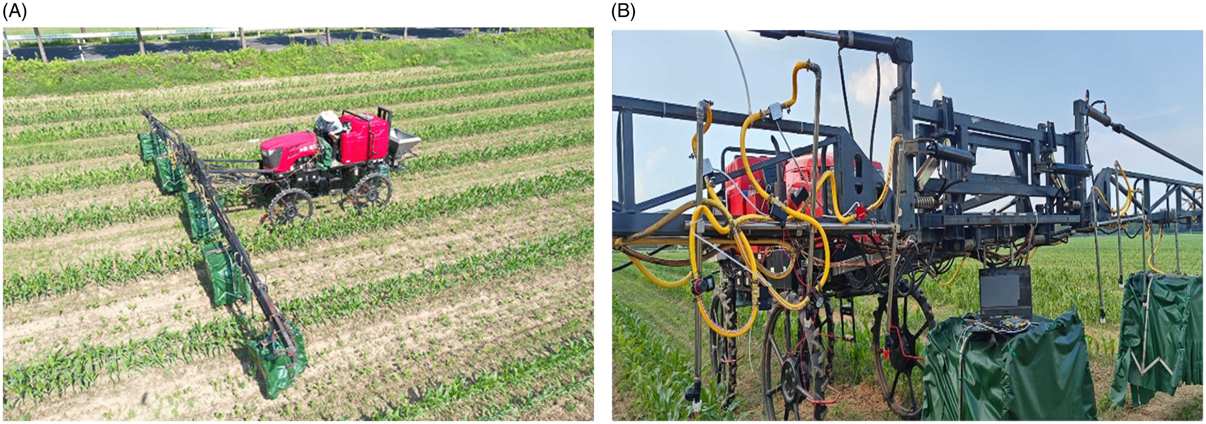


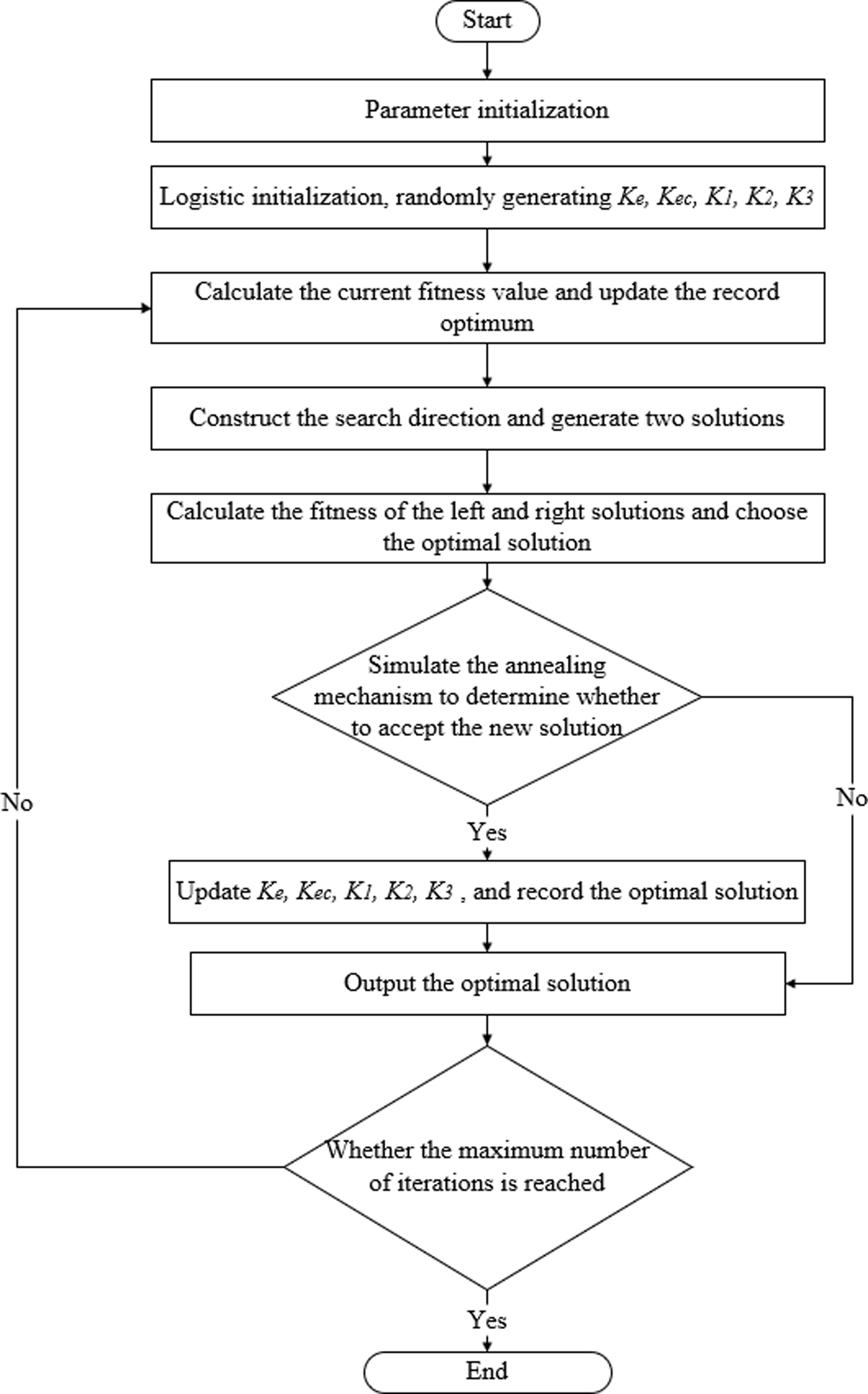


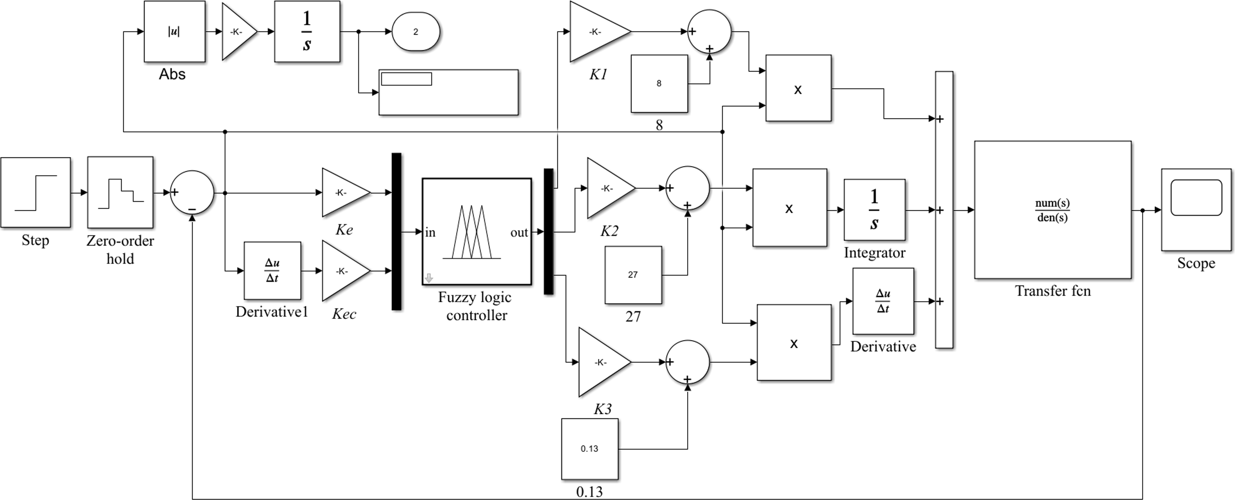


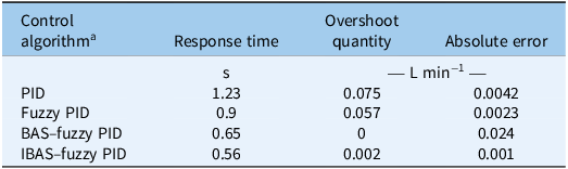
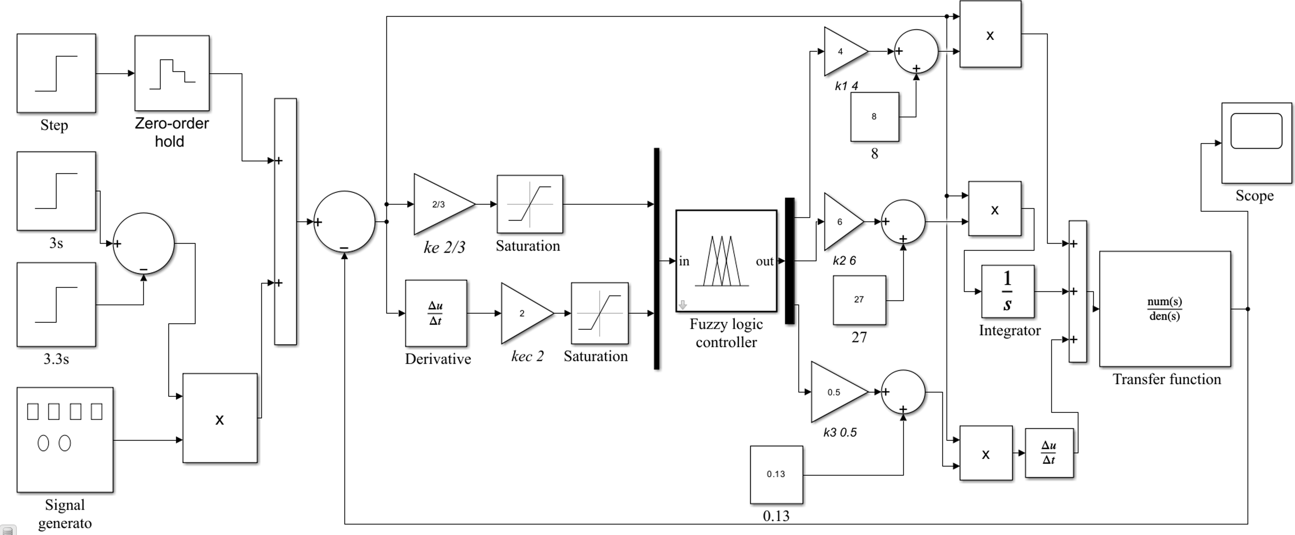


 Open access