


1. Introduction
Wall-bounded turbulence over complex geometries arises in many engineering and geophysical contexts, ranging from aircraft wings and turbine blades to ships, atmospheric boundary layers and wind farms. Because high-fidelity numerical tools such as direct numerical simulations (DNS) are prohibitively costly at practically relevant Reynolds numbers (Choi & Moin Reference Choi and Moin2012; Yang & Griffin Reference Yang and Griffin2021), modelling is often the only practical option. Yet turbulence models frequently fail to capture the intricate physics of these flows. Effects such as streamline curvature, pressure gradients and flow separation remain challenging, and it is often unclear which aspects of the flow physics are inadequately represented in a given model (Huang et al. Reference Huang, Chyczewski, Xia, Kunz and Yang2023). Addressing this gap requires an error diagnostic framework that attributes modelling errors to distinct physical mechanisms arising from the underlying assumptions and calibrations.
A natural starting point for such an error diagnostic framework is the skin-friction coefficient $C_{\!f}$
, a fundamental engineering quantity that reflects the combined influence of several underlying physical mechanisms. Over the past two decades, a variety of decomposition frameworks have provided insight into these processes. The seminal work of Fukagata, Iwamoto & Kasagi (Reference Fukagata, Iwamoto and Kasagi2002) introduced the now well-known FIK decomposition, which clarified the distinct contributions of different flow processes to
$C_{\!f}$
, a fundamental engineering quantity that reflects the combined influence of several underlying physical mechanisms. Over the past two decades, a variety of decomposition frameworks have provided insight into these processes. The seminal work of Fukagata, Iwamoto & Kasagi (Reference Fukagata, Iwamoto and Kasagi2002) introduced the now well-known FIK decomposition, which clarified the distinct contributions of different flow processes to $C_{\!f}$
. Other
$C_{\!f}$
. Other $C_{\!f}$
decompositions include formulations based on the kinetic energy integral (Renard & Deck Reference Renard and Deck2016), the angular momentum integral (AMI) (Elnahhas & Johnson Reference Elnahhas and Johnson2022), extensions for rough-wall flows (Zhang et al. Reference Zhang, Yang, Chen and Wan2024), and formulations for flow outside the wall layer (Volino & Schultz Reference Volino and Schultz2018; Xia, Zhang & Yang Reference Xia, Zhang and Yang2021). The AMI-based formulation, in particular, decomposes
$C_{\!f}$
decompositions include formulations based on the kinetic energy integral (Renard & Deck Reference Renard and Deck2016), the angular momentum integral (AMI) (Elnahhas & Johnson Reference Elnahhas and Johnson2022), extensions for rough-wall flows (Zhang et al. Reference Zhang, Yang, Chen and Wan2024), and formulations for flow outside the wall layer (Volino & Schultz Reference Volino and Schultz2018; Xia, Zhang & Yang Reference Xia, Zhang and Yang2021). The AMI-based formulation, in particular, decomposes $C_{\!f}$
into contributions from viscous effects, Reynolds shear stress, total mean flux, free-stream pressure gradients, and terms associated with departures from the boundary-layer approximation. Unlike classical FIK-type relations applied to boundary layers, this approach isolates the viscous term as skin friction of the equivalent laminar boundary layer (Blasius Reference Blasius1907) in a single Reynolds-number-dependent term. This enables a clear interpretation of the remaining terms as augmentations relative to a well-defined laminar reference state. Furthermore, the AMI method remains well defined and physically interpretable even in regions of flow separation and recirculation, and has been applied to flows over Gaussian bumps and aerofoils with both favourable and adverse pressure gradients (Kianfar & Johnson Reference Kianfar and Johnson2025). Despite these advances, existing formulations – including the FIK and AMI decompositions – remain largely restricted to two-dimensional mean flows, with extensions to three-dimensional configurations of engineering relevance still rare. Moreover, most integral decompositions have so far been used mainly for post-processing of high-fidelity data, rather than as diagnostic tools for turbulence models. The present study addresses these gaps by extending
$C_{\!f}$
into contributions from viscous effects, Reynolds shear stress, total mean flux, free-stream pressure gradients, and terms associated with departures from the boundary-layer approximation. Unlike classical FIK-type relations applied to boundary layers, this approach isolates the viscous term as skin friction of the equivalent laminar boundary layer (Blasius Reference Blasius1907) in a single Reynolds-number-dependent term. This enables a clear interpretation of the remaining terms as augmentations relative to a well-defined laminar reference state. Furthermore, the AMI method remains well defined and physically interpretable even in regions of flow separation and recirculation, and has been applied to flows over Gaussian bumps and aerofoils with both favourable and adverse pressure gradients (Kianfar & Johnson Reference Kianfar and Johnson2025). Despite these advances, existing formulations – including the FIK and AMI decompositions – remain largely restricted to two-dimensional mean flows, with extensions to three-dimensional configurations of engineering relevance still rare. Moreover, most integral decompositions have so far been used mainly for post-processing of high-fidelity data, rather than as diagnostic tools for turbulence models. The present study addresses these gaps by extending $C_{\!f}$
decomposition frameworks to three-dimensional turbulent boundary layers (TBLs) and exploring their potential as an error diagnostic tool for turbulence model evaluation and improvement.
$C_{\!f}$
decomposition frameworks to three-dimensional turbulent boundary layers (TBLs) and exploring their potential as an error diagnostic tool for turbulence model evaluation and improvement.
On the modelling side, $C_{\!f}$
has long served as a benchmark metric (Launder & Spalding Reference Launder and Spalding1974; Bose & Park Reference Bose and Park2018), with emphasis placed on matching its magnitude to experimental or DNS results. In the context of wall-modelled large-eddy simulations (WMLES), various forms of log-layer mismatch can introduce 10–15 % error in predicted skin friction, motivating remedies such as random forcing (DeLeon & Senocak Reference DeLeon and Senocak2019), filtering (Bou-Zeid, Meneveau & Parlange Reference Bou-Zeid, Meneveau and Parlange2004; Yang, Park & Moin Reference Yang, Park and Moin2017), displaced LES/wall-model matching (Kawai & Larsson Reference Kawai and Larsson2012; Shin, Yang & Howland Reference Shin, Yang and Howland2025), among others (Maejima, Tanino & Kawai Reference Maejima, Tanino and Kawai2024; Yang, Abkar & Park Reference Yang, Abkar and Park2024; Liu et al. Reference Liu, Yang, Shi and Chen2025). More recently, data-driven approaches have also targeted
$C_{\!f}$
has long served as a benchmark metric (Launder & Spalding Reference Launder and Spalding1974; Bose & Park Reference Bose and Park2018), with emphasis placed on matching its magnitude to experimental or DNS results. In the context of wall-modelled large-eddy simulations (WMLES), various forms of log-layer mismatch can introduce 10–15 % error in predicted skin friction, motivating remedies such as random forcing (DeLeon & Senocak Reference DeLeon and Senocak2019), filtering (Bou-Zeid, Meneveau & Parlange Reference Bou-Zeid, Meneveau and Parlange2004; Yang, Park & Moin Reference Yang, Park and Moin2017), displaced LES/wall-model matching (Kawai & Larsson Reference Kawai and Larsson2012; Shin, Yang & Howland Reference Shin, Yang and Howland2025), among others (Maejima, Tanino & Kawai Reference Maejima, Tanino and Kawai2024; Yang, Abkar & Park Reference Yang, Abkar and Park2024; Liu et al. Reference Liu, Yang, Shi and Chen2025). More recently, data-driven approaches have also targeted $C_{\!f}$
. For example, Hu et al. (Reference Hu, Huang, Kunz and Yang2025) developed low-Reynolds-number corrections to the
$C_{\!f}$
. For example, Hu et al. (Reference Hu, Huang, Kunz and Yang2025) developed low-Reynolds-number corrections to the $k$
–
$k$
– $\epsilon$
model that improve
$\epsilon$
model that improve $C_{\!f}$
predictions in boundary layers with pressure gradients, and Bae & Koumoutsakos (Reference Bae and Koumoutsakos2022) applied reinforcement learning and trained wall models that capture
$C_{\!f}$
predictions in boundary layers with pressure gradients, and Bae & Koumoutsakos (Reference Bae and Koumoutsakos2022) applied reinforcement learning and trained wall models that capture $C_{\!f}$
in plane channel flow as well as separated periodic hill flows. Indeed, most machine-learned closures have relied on
$C_{\!f}$
in plane channel flow as well as separated periodic hill flows. Indeed, most machine-learned closures have relied on $C_{\!f}$
as a validation quantity (Parish & Duraisamy Reference Parish and Duraisamy2016; Ahmed et al. Reference Ahmed, Menon, Sitarski, Sharma and Durbin2025; Wu, Zhang & Zhang Reference Wu, Zhang and Zhang2025; Yang et al. Reference Yang, Shan, Yang and Zhang2025). In rough-wall flows, recent reviews noted that predictive methods remain uncertain by at least 10 % (Chung et al. Reference Chung, Hutchins, Schultz and Flack2021; Yang et al. Reference Yang, Zhang, Yuan and Kunz2023), underscoring the continuing emphasis on skin-friction matching in turbulence model development. However, while accurate
$C_{\!f}$
as a validation quantity (Parish & Duraisamy Reference Parish and Duraisamy2016; Ahmed et al. Reference Ahmed, Menon, Sitarski, Sharma and Durbin2025; Wu, Zhang & Zhang Reference Wu, Zhang and Zhang2025; Yang et al. Reference Yang, Shan, Yang and Zhang2025). In rough-wall flows, recent reviews noted that predictive methods remain uncertain by at least 10 % (Chung et al. Reference Chung, Hutchins, Schultz and Flack2021; Yang et al. Reference Yang, Zhang, Yuan and Kunz2023), underscoring the continuing emphasis on skin-friction matching in turbulence model development. However, while accurate $C_{\!f}$
prediction suggests improved representation of near-wall dynamics, it does not guarantee overall model fidelity: because
$C_{\!f}$
prediction suggests improved representation of near-wall dynamics, it does not guarantee overall model fidelity: because $C_{\!f}$
reflects the combined action of multiple physical processes, the correct magnitude may arise from compensating errors among them. This study therefore seeks to bridge this gap by assessing how turbulence models represent the individual mechanisms that contribute to
$C_{\!f}$
reflects the combined action of multiple physical processes, the correct magnitude may arise from compensating errors among them. This study therefore seeks to bridge this gap by assessing how turbulence models represent the individual mechanisms that contribute to $C_{\!f}$
. Further, we emphasise that the present study does not challenge the established turbulence modelling framework of Reynolds-averaged Navier–Stokes (RANS) closures, which are designed primarily to reproduce mean-flow quantities with acceptable engineering accuracy. Rather, we propose a mechanism-resolved diagnostic framework that complements conventional validation by revealing how individual physical processes combine to produce the predicted aggregate
$C_{\!f}$
. Further, we emphasise that the present study does not challenge the established turbulence modelling framework of Reynolds-averaged Navier–Stokes (RANS) closures, which are designed primarily to reproduce mean-flow quantities with acceptable engineering accuracy. Rather, we propose a mechanism-resolved diagnostic framework that complements conventional validation by revealing how individual physical processes combine to produce the predicted aggregate $C_{\!f}$
. For instance, a model may predict the correct total
$C_{\!f}$
. For instance, a model may predict the correct total $C_{\!f}$
through compensating errors, where an overprediction in one mechanism (e.g. turbulent torque) is offset by an underprediction in another (e.g. mean-flux contribution). Conversely, multiple small errors may compound and lead to significant deviations in skin friction. Identifying such distinctions is important because if a known physical deficiency contributes to error cancellation, then correcting it in isolation may actually degrade the overall prediction. In this sense, accurate
$C_{\!f}$
through compensating errors, where an overprediction in one mechanism (e.g. turbulent torque) is offset by an underprediction in another (e.g. mean-flux contribution). Conversely, multiple small errors may compound and lead to significant deviations in skin friction. Identifying such distinctions is important because if a known physical deficiency contributes to error cancellation, then correcting it in isolation may actually degrade the overall prediction. In this sense, accurate $C_{\!f}$
is viewed as informative but not by itself sufficient in representing its underlying physical contributions.
$C_{\!f}$
is viewed as informative but not by itself sufficient in representing its underlying physical contributions.
The phenomenon of error cancellation has been highlighted in previous studies. For instance, Klemmer & Mueller (Reference Klemmer and Mueller2021) derived a transport equation for the model-form error in RANS by comparing the exact Reynolds stress tensor with that modelled using the Boussinesq eddy-viscosity hypothesis. Their analysis of channel flows revealed fortuitous cancellation between the Boussinesq approximation and the modelled transport equations: an underestimation of $k$
and overestimation of
$k$
and overestimation of $\epsilon$
combine to yield more accurate eddy viscosity
$\epsilon$
combine to yield more accurate eddy viscosity $\nu _t$
in both
$\nu _t$
in both $k$
–
$k$
– $\epsilon$
and
$\epsilon$
and $k$
–
$k$
– $\omega$
closures. Despite being fundamentally less accurate, the
$\omega$
closures. Despite being fundamentally less accurate, the $k$
–
$k$
– $\omega$
model outperformed the
$\omega$
model outperformed the $k$
–
$k$
– $\epsilon$
model in a posteriori predictions of mean velocity profiles and turbulent shear stress, owing to more effective redistribution of errors. Extending this analysis, Klemmer, Wu & Mueller (Reference Klemmer, Wu and Mueller2023) showed similar behaviour in turbulent planar jets and separation bubbles, identifying two distinct modes of error cancellation associated with wall-bounded and free-shear flows. These findings further underscore the need to quantify modelling errors in terms of distinct physical mechanisms.
$\epsilon$
model in a posteriori predictions of mean velocity profiles and turbulent shear stress, owing to more effective redistribution of errors. Extending this analysis, Klemmer, Wu & Mueller (Reference Klemmer, Wu and Mueller2023) showed similar behaviour in turbulent planar jets and separation bubbles, identifying two distinct modes of error cancellation associated with wall-bounded and free-shear flows. These findings further underscore the need to quantify modelling errors in terms of distinct physical mechanisms.
In this study, we combine the AMI-based $C_{\!f}$
decomposition with high-fidelity datasets to isolate and quantify the contributions of individual flow processes to turbulence model error. Instead of treating
$C_{\!f}$
decomposition with high-fidelity datasets to isolate and quantify the contributions of individual flow processes to turbulence model error. Instead of treating $C_{\!f}$
as a single scalar benchmark, we decompose it into interpretable terms that reveal which mechanisms – such as Reynolds shear stress, free-stream pressure gradients or boundary-layer growth – are misrepresented by a given model. To demonstrate this approach, we examine two flow configurations: the canonical flat-plate TBL, which serves as a baseline for establishing the methodology, and TBL flow over the asymmetric three-dimensional BeVERLI (benchmark validation experiments for RANS and LES investigations) hill (Gargiulo et al. Reference Gargiulo, Beardsley, Vishwanathan, Fritsch, Duetsch-Patel, Szoke, Borgoltz, Devenport, Roy and Lowe2020). Previous validation studies of the symmetric BeVERLI hill have revealed significant RANS–experiment discrepancies in predicting separation and vortex shedding (Gargiulo et al. Reference Gargiulo, Duetsch-Patel, Ozoroski, Beardsley, Vishwanathan, Fritsch, Borgoltz, Devenport, Roy and Lowe2021, Reference Gargiulo2022; Williams et al. Reference Williams, Annamalai, Ozoroski, Roy and Lowe2022). Here, we extend the analysis to the asymmetric geometry, using wall-resolved large-eddy simulations (WRLES) as the high-fidelity reference, and the AMI-based framework as the error diagnostic tool. In doing so, we address two complementary challenges: the application challenge of extending
$C_{\!f}$
as a single scalar benchmark, we decompose it into interpretable terms that reveal which mechanisms – such as Reynolds shear stress, free-stream pressure gradients or boundary-layer growth – are misrepresented by a given model. To demonstrate this approach, we examine two flow configurations: the canonical flat-plate TBL, which serves as a baseline for establishing the methodology, and TBL flow over the asymmetric three-dimensional BeVERLI (benchmark validation experiments for RANS and LES investigations) hill (Gargiulo et al. Reference Gargiulo, Beardsley, Vishwanathan, Fritsch, Duetsch-Patel, Szoke, Borgoltz, Devenport, Roy and Lowe2020). Previous validation studies of the symmetric BeVERLI hill have revealed significant RANS–experiment discrepancies in predicting separation and vortex shedding (Gargiulo et al. Reference Gargiulo, Duetsch-Patel, Ozoroski, Beardsley, Vishwanathan, Fritsch, Borgoltz, Devenport, Roy and Lowe2021, Reference Gargiulo2022; Williams et al. Reference Williams, Annamalai, Ozoroski, Roy and Lowe2022). Here, we extend the analysis to the asymmetric geometry, using wall-resolved large-eddy simulations (WRLES) as the high-fidelity reference, and the AMI-based framework as the error diagnostic tool. In doing so, we address two complementary challenges: the application challenge of extending $C_{\!f}$
decompositions to complex three-dimensional TBLs, and the methodological challenge of attributing RANS model errors in skin friction to individual physical mechanisms.
$C_{\!f}$
decompositions to complex three-dimensional TBLs, and the methodological challenge of attributing RANS model errors in skin friction to individual physical mechanisms.
The rest of the paper is organised as follows. In § 2, we present the integral analysis based on the AMI technique applied to three-dimensional flows, followed by the error-analysis framework for turbulence models and an aleatory uncertainty quantification method. Details of the datasets are given in § 3, including the computational domain, grid and boundary conditions for the flat-plate TBL and the three-dimensional bump cases. Results are presented in § 4, and conclusions are drawn in § 5.
2. Methodology
We extend the AMI framework of Elnahhas & Johnson (Reference Elnahhas and Johnson2022) to three-dimensional mean flows in § 2.1, and formulate the corresponding error-analysis methodology in § 2.2. We also introduce an aleatory uncertainty quantification method in § 2.3.
2.1. The AMI for three-dimensional mean flow
First, the free-stream momentum equation is given by
 \begin{align} \frac {\partial U}{\partial t}+U \frac {\partial U}{\partial x} + V \frac {\partial U}{\partial y} + W \frac {\partial U}{\partial z}=-\frac {1}{\rho } \frac {\partial P}{\partial x} + \nu \left [ \frac {\partial ^2 U}{\partial x^2}+ \frac {\partial ^2 U}{\partial y^2}+\frac {\partial ^2 U}{\partial z^2}\right ]\!, \end{align}
where $U$
,
$U$
, $V$
and
$V$
and $W$
denote the inviscid streamwise, wall-normal and spanwise velocity components in the absence of a boundary layer and turbulence. These flow variables do not satisfy the no-slip boundary condition at the wall. To reconstruct the streamwise free-stream velocity
$W$
denote the inviscid streamwise, wall-normal and spanwise velocity components in the absence of a boundary layer and turbulence. These flow variables do not satisfy the no-slip boundary condition at the wall. To reconstruct the streamwise free-stream velocity $U$
, we follow Kianfar & Johnson (Reference Kianfar and Johnson2025) and use the irrotational, inviscid solution from the Bernoulli equation (Griffin, Fu & Moin Reference Griffin, Fu and Moin2021),
$U$
, we follow Kianfar & Johnson (Reference Kianfar and Johnson2025) and use the irrotational, inviscid solution from the Bernoulli equation (Griffin, Fu & Moin Reference Griffin, Fu and Moin2021),
 \begin{align} U = \pm \sqrt {\frac {2}{\rho } \left ( P_{o,{\textit{ref}}} - P \right ) - V^2 - W^2}, \end{align}
where the reference pressure $P_{o,{\textit{ref}}}$
is taken as the maximum stagnation pressure, nearly constant in the free stream. In practice,
$P_{o,{\textit{ref}}}$
is taken as the maximum stagnation pressure, nearly constant in the free stream. In practice, $V$
and
$V$
and $W$
are taken from the corresponding viscous flow and are negligible in the free stream.
$W$
are taken from the corresponding viscous flow and are negligible in the free stream.
In the presence of a boundary layer and turbulence effects, the mean continuity and streamwise momentum equations for incompressible three-dimensional flow are
 \begin{align} \frac {\partial \bar {u}}{\partial x}+\frac {\partial \bar {v}}{\partial y}+\frac {\partial \bar {w}}{\partial z}&=0, \end{align}
 \begin{align} \frac {\partial \bar {u}}{\partial t}+\frac {\partial \bar {u}^2}{\partial x}+\frac {\partial \bar {u} \bar {v}}{\partial y}+\frac {\partial \bar {u} \bar {w}}{\partial z} &= -\frac {1}{\rho } \frac {\partial \bar {p}}{\partial x}+ \nu \left [ \frac {\partial ^2 \bar {u}}{\partial x^2}+ \frac {\partial ^2 \bar {u}}{\partial y^2}+\frac {\partial ^2 \bar {u}}{\partial z^2}\right ]\nonumber\\&\quad -\left [\frac {\partial \overline {u^{\prime 2}}}{\partial x}+\frac {\partial \overline {u^{\prime } v^{\prime }}}{\partial y}+\frac {\partial \overline {u^{\prime } w^{\prime }}}{\partial z}\right ]\!, \end{align}
where $x$
,
$x$
, $y$
and
$y$
and $z$
denote streamwise, wall-normal and spanwise directions, respectively, with
$z$
denote streamwise, wall-normal and spanwise directions, respectively, with $u$
,
$u$
, $v$
and
$v$
and $w$
being the velocities in these directions. Subtracting (2.4) from (2.1) and adding
$w$
being the velocities in these directions. Subtracting (2.4) from (2.1) and adding $(U - \bar {u})$
times (2.3) gives the streamwise momentum deficit equation:
$(U - \bar {u})$
times (2.3) gives the streamwise momentum deficit equation:

where

denotes terms that lead to departure from boundary-layer approximation. The terms enclosed in red boxes are due to mean-flow three-dimensionality. These are additional terms that extend the two-dimensional AMI method in Elnahhas & Johnson (Reference Elnahhas and Johnson2022) to incorporate spanwise effects for application to three-dimensional geometries. It is also important to note that both (2.1) and (2.4) are evaluated at the same spatial locations – the former reconstructed from the inviscid solution, and the latter valid throughout the domain – so the subtraction is performed locally within the same physical domain rather than between disjoint regions.
The AMI equation can then be constructed by multiplying (2.5) by $(y-\ell )/(U_{io}^2 \ell )$
and integrating from
$(y-\ell )/(U_{io}^2 \ell )$
and integrating from $0$
to
$0$
to $\infty$
:
$\infty$
:

where
 \begin{align} {\textit{Re}}_{\ell }=U_{io} \ell / v,\ \mathcal{I}^{\ell } \equiv \int _0^{\infty }\left (1-\frac {y}{\ell }\right ) \frac {I_x}{U_{io}^2}\, \mathrm{d} y, \end{align}
and the normalising velocity $U_{io}$
comes from the irrotational solution evaluated at the wall,
$U_{io}$
comes from the irrotational solution evaluated at the wall, $U_{io} = U(y=0)$
(Kianfar, Elnahhas & Johnson Reference Kianfar, Elnahhas and Johnson2023). The boundary-layer momentum thicknesses are
$U_{io} = U(y=0)$
(Kianfar, Elnahhas & Johnson Reference Kianfar, Elnahhas and Johnson2023). The boundary-layer momentum thicknesses are
 \begin{align} \quad \theta _x \equiv \int _0^{\infty }\left (\frac {U-\bar {u}(y)}{U_{io}}\right ) \frac {\bar {u}(y)}{U_{io}}\, \mathrm{d} y, \quad \theta _z \equiv \int _0^{\infty }\left (\frac {U-\bar {u}(y)}{U_{io}}\right ) \frac {\bar {w}(y)}{U_{io}}\, \mathrm{d} y. \end{align}
The momentum and displacement thicknesses based on the length scale $\ell$
are
$\ell$
are
 \begin{align} \begin{aligned} \delta _{\ell _x}^* &\equiv \int _{0}^{\infty } \left (1 - \frac {y}{\ell }\right ) \left (\frac {U - \bar {u}}{U_{io}}\right ) \, \mathrm{d}y, \\\theta _{\ell _x} &\equiv \int _{0}^{\infty } \left (1 - \frac {y}{\ell }\right ) \frac {\bar {u}}{U_{io}} \left (\frac {U - \bar {u}}{U_{io}}\right ) \, \mathrm{d}y,\\\theta _{\ell _z} &\equiv \int _{0}^{\infty } \left (1 - \frac {y}{\ell }\right ) \frac {\bar {w}}{U_{io}} \left (\frac {U - \bar {u}}{U_{io}}\right ) \, \mathrm{d}y,\\\theta _{v} &\equiv \int _{0}^{\infty } \left (1 - \frac {y}{\ell }\right ) \frac {\bar {v}}{U_{io}} \left (\frac {U - \bar {u}}{U_{io}}\right ) \, \mathrm{d}y .\\\end{aligned} \end{align}
The length scale $\ell$
can be thought of as the point about which these torques due to various
$\ell$
can be thought of as the point about which these torques due to various $C_{\!f}$
contributions act on the TBL. Its value is chosen to be 4.54 times the streamwise momentum thickness (
$C_{\!f}$
contributions act on the TBL. Its value is chosen to be 4.54 times the streamwise momentum thickness ( $\theta _x$
), following Kianfar & Johnson (Reference Kianfar and Johnson2025).
$\theta _x$
), following Kianfar & Johnson (Reference Kianfar and Johnson2025).
Equation (2.7) constitutes the AMI decomposition of the skin-friction coefficient,
 \begin{align} C_{\!f} \equiv \frac {\tau _w}{\dfrac {1}{2} \rho U_{io}^2}, \end{align}
where $\tau _w$
is the wall shear stress. The first term on the right-hand side of (2.7) represents the viscous contribution, obtained by comparing the TBL with an equivalent laminar boundary layer at the same Reynolds number. This
$\tau _w$
is the wall shear stress. The first term on the right-hand side of (2.7) represents the viscous contribution, obtained by comparing the TBL with an equivalent laminar boundary layer at the same Reynolds number. This $1/{\textit{Re}}_{\ell }$
term is also referred to as the ‘laminar friction’ term (Elnahhas & Johnson Reference Elnahhas and Johnson2022; Kianfar & Johnson Reference Kianfar and Johnson2025), corresponding to the wall shear that would arise from molecular diffusion alone in the absence of turbulent momentum transport. The length scale
$1/{\textit{Re}}_{\ell }$
term is also referred to as the ‘laminar friction’ term (Elnahhas & Johnson Reference Elnahhas and Johnson2022; Kianfar & Johnson Reference Kianfar and Johnson2025), corresponding to the wall shear that would arise from molecular diffusion alone in the absence of turbulent momentum transport. The length scale $\ell$
denotes the centre of action of this viscous contribution in the reference laminar boundary layer, and does not imply the existence of a laminar region within the TBL. The second term quantifies the turbulent torque, capturing the enhancement of wall shear stress due to momentum transfer by turbulent fluctuations. The following five terms arise from mean-flow fluxes associated with streamwise and spanwise growth of the boundary layer; these typically reduce skin friction, as boundary-layer thickening carries momentum away from the wall, and offsets turbulent enhancement. The next two terms represent free-stream pressure-gradient effects: a favourable pressure gradient increases
$\ell$
denotes the centre of action of this viscous contribution in the reference laminar boundary layer, and does not imply the existence of a laminar region within the TBL. The second term quantifies the turbulent torque, capturing the enhancement of wall shear stress due to momentum transfer by turbulent fluctuations. The following five terms arise from mean-flow fluxes associated with streamwise and spanwise growth of the boundary layer; these typically reduce skin friction, as boundary-layer thickening carries momentum away from the wall, and offsets turbulent enhancement. The next two terms represent free-stream pressure-gradient effects: a favourable pressure gradient increases $C_{\!f}$
by accelerating the free stream, whereas an adverse gradient reduces it. Finally, residual contributions due to unsteadiness, three-dimensionality, or other departures from ideal two-dimensional conditions are collected into
$C_{\!f}$
by accelerating the free stream, whereas an adverse gradient reduces it. Finally, residual contributions due to unsteadiness, three-dimensionality, or other departures from ideal two-dimensional conditions are collected into $\mathcal{I}^{\ell }$
, which is negligible for steady, zero-pressure-gradient flat-plate flows.
$\mathcal{I}^{\ell }$
, which is negligible for steady, zero-pressure-gradient flat-plate flows.
Alternative but mathematically equivalent regroupings of the terms in (2.7) are possible. These are discussed in Appendix A, where we demonstrate that the principal qualitative trends remain robust under such rearrangements.
2.2. The AMI-enabled error analysis
The AMI framework enables a term-by-term decomposition of modelling error by associating each contribution to $C_{\!f}$
with a distinct physical mechanism. More generally, any quantity of interest (QoI) may be expressed as the sum of such contributions. For a high-fidelity reference solution, such as DNS or WRLES, we may write
$C_{\!f}$
with a distinct physical mechanism. More generally, any quantity of interest (QoI) may be expressed as the sum of such contributions. For a high-fidelity reference solution, such as DNS or WRLES, we may write
 \begin{align} \mathrm{QoI}_{{\textit{ref}}} = \sum _{i} C_i^{{\textit{ref}}}, \end{align}
where $C_i^{{\textit{ref}}}$
denotes the contribution of the
$C_i^{{\textit{ref}}}$
denotes the contribution of the $i$
th physical mechanism, evaluated from the reference flow field. For a lower-fidelity model prediction, e.g. RANS, the same QoI can be expressed as
$i$
th physical mechanism, evaluated from the reference flow field. For a lower-fidelity model prediction, e.g. RANS, the same QoI can be expressed as
 \begin{align} \mathrm{QoI}_{{M}} = \sum _{i} C_i^{{M}}, \end{align}
where $C_i^{{M}}$
is the corresponding contribution obtained from the modelled flow field. The discrepancy between the two is therefore
$C_i^{{M}}$
is the corresponding contribution obtained from the modelled flow field. The discrepancy between the two is therefore
 \begin{align} \mathrm{QoI}_{{M}} - \mathrm{QoI}_{{\textit{ref}}} = \sum _{i}\left ( C_i^{{M}} - C_i^{{\textit{ref}}} \right )\!, \end{align}
showing explicitly that the total error arises from the sum of term-by-term differences in the underlying physical contributions. This additive structure naturally motivates an error-budget interpretation: each mechanism contributes a separate component of error, which may reinforce or cancel others.
Here, the QoI is the skin-friction coefficient $C_{\!f}$
, and its decomposition is given by the AMI:
$C_{\!f}$
, and its decomposition is given by the AMI:
 \begin{align} \frac {\Delta C_{\!f}}{2} ={}& \underbrace {\varDelta \left ( \frac {1}{{\textit{Re}}_\ell } \right )}_{\text{laminar friction}} + \underbrace {\varDelta \left ( \int _0^{\infty } \frac {-\overline {u^{\prime } v^{\prime }}}{U_{io}^2 \ell } \, \mathrm{d}y \right )}_{\text{turbulent torque}} \nonumber \\ &+ \underbrace {\varDelta \left ( \frac {\partial \theta _{\ell x}}{\partial x} - \frac {\theta _x - \theta _{\ell _x}}{\ell } \frac {\mathrm{d}\ell }{\mathrm{d}x} + \frac {\partial \theta _{\ell z}}{\partial z} - \frac {\theta _z - \theta _{\ell _z}}{\ell } \frac {\mathrm{d}\ell }{\mathrm{d}z} + \frac {\theta _v}{\ell } \right )}_{\text{Total mean flux}} \nonumber \\ &+ \underbrace {\varDelta \left ( \frac {\delta _{\ell _x}^* + 2 \theta _{\ell _x}}{U_{io}} \frac {\partial U}{\partial x} + \frac {2 \theta _{\ell _z}}{U_{io}} \frac {\partial U}{\partial z} \right )}_{\text{Pressure-gradient effects}} + \underbrace {\varDelta \big ( \mathcal{I}^{\ell } \big )}_{\text{Departure from boundary-layer approximation}}. \end{align}
Here, $\Delta$
denotes the difference between the turbulence model prediction and the high-fidelity reference. For example, the error in
$\Delta$
denotes the difference between the turbulence model prediction and the high-fidelity reference. For example, the error in $C_{\!f}$
from the
$C_{\!f}$
from the $k{-}\omega$
shear-stress transport (SST) model relative to WRLES is
$k{-}\omega$
shear-stress transport (SST) model relative to WRLES is
 \begin{align} \Delta C_{\!f,{\textit{SST}}}/2 = C_{\!f,{\textit{SST}}}/2 - C_{\!f,{\textit{WRLES}}}/2. \end{align}
Equation (2.15) thus provides a systematic decomposition of skin-friction error into contributions from individual physical processes. In this study, we apply this framework to five RANS models, i.e. the two-equation $k{-}\omega$
SST model (Menter Reference Menter1994), Chien’s
$k{-}\omega$
SST model (Menter Reference Menter1994), Chien’s $k$
–
$k$
– $\epsilon$
model (Chien Reference Chien1982), the one-equation Spalart–Allmaras (SA) model (Spalart Reference Spalart1988), the four-equation
$\epsilon$
model (Chien Reference Chien1982), the one-equation Spalart–Allmaras (SA) model (Spalart Reference Spalart1988), the four-equation $v^2{-}f$
model (Laurence, Uribe & Utyuzhnikov Reference Laurence, Uribe and Utyuzhnikov2005) and the Reynolds-stress-based Speziale-Sarkar-Gatski/Launder-Reece-Rodi (SSG-LRR) model (Eisfeld, Rumsey & Togiti Reference Eisfeld, Rumsey and Togiti2016), and two flow configurations, i.e. the flat-plate TBL and the BeVERLI hill.
$v^2{-}f$
model (Laurence, Uribe & Utyuzhnikov Reference Laurence, Uribe and Utyuzhnikov2005) and the Reynolds-stress-based Speziale-Sarkar-Gatski/Launder-Reece-Rodi (SSG-LRR) model (Eisfeld, Rumsey & Togiti Reference Eisfeld, Rumsey and Togiti2016), and two flow configurations, i.e. the flat-plate TBL and the BeVERLI hill.
2.3. Aleatory uncertainty quantification
Previous studies (Kianfar et al. Reference Kianfar, Elnahhas and Johnson2023; Kianfar & Johnson Reference Kianfar and Johnson2025) emphasised that incomplete statistical convergence of turbulent boundary-layer data introduces errors that directly affect AMI analyses. For the zero-pressure-gradient flat-plate DNS of Wu et al. (Reference Wu, Moin, Wallace, Skarda, Lozano-Durán and Hickey2017), the AMI equation balanced the skin-friction coefficient with average discrepancy 1.4 %. This deviation was traced to the amplification of statistical noise by streamwise derivatives, which are especially sensitive to finite sampling (Kianfar et al. Reference Kianfar, Elnahhas and Johnson2023). In Kianfar & Johnson (Reference Kianfar and Johnson2025), a normalised residual was introduced and shown to increase in regions of strong pressure gradients, growing markedly near incipient separation where unsteady dynamics produces noisier statistics. Both studies identified streamwise derivatives as the dominant source of error amplification, with additional contributions from wall-normal integrals and edge definitions.
To systematically assess the susceptibility of AMI terms to convergence errors, we introduce controlled synthetic perturbations that emulate noise in the data. The perturbations are constructed to be divergence-free, to have a prescribed magnitude and to obey a Kolmogorov $k^{-5/3}$
spectrum. The resulting noisy velocity fields are then used to recompute the AMI terms, and the differences provide estimates of the sensitivity of each contribution to sampling error. In particular, adding noise to converged RANS solutions offers a clean baseline, since RANS solutions are free from temporal-averaging error.
$k^{-5/3}$
spectrum. The resulting noisy velocity fields are then used to recompute the AMI terms, and the differences provide estimates of the sensitivity of each contribution to sampling error. In particular, adding noise to converged RANS solutions offers a clean baseline, since RANS solutions are free from temporal-averaging error.
The procedure is as follows. Consider two-dimensional mean flow. Incompressibility is enforced by introducing a scalar stream function $\psi (x,y)$
, with perturbation velocities
$\psi (x,y)$
, with perturbation velocities
 \begin{align} e'_u=\frac {\partial \psi }{\partial y},\quad e'_v=-\frac {\partial \psi }{\partial x}. \end{align}
In Fourier space on a periodic domain $(L_x,L_y)$
with wavenumbers
$(L_x,L_y)$
with wavenumbers $k_x=2\pi n_x/L_x$
,
$k_x=2\pi n_x/L_x$
, $k_y=2\pi n_y/L_y$
and
$k_y=2\pi n_y/L_y$
and $\boldsymbol{k}=(k_x,k_y)$
, this becomes
$\boldsymbol{k}=(k_x,k_y)$
, this becomes
 \begin{align} \widehat {e'_u}(\boldsymbol{k}) = {\rm i}\,k_y\,\widehat {\psi }(\boldsymbol{k}),\quad \widehat {e'_v}(\boldsymbol{k}) = -{\rm i}\,k_x\,\widehat {\psi }(\boldsymbol{k}), \end{align}
so that $\boldsymbol{k}\boldsymbol{\cdot }\widehat {\boldsymbol{e'}}(\boldsymbol{k})=0$
, ensuring the divergence-free constraint. To enforce the
$\boldsymbol{k}\boldsymbol{\cdot }\widehat {\boldsymbol{e'}}(\boldsymbol{k})=0$
, ensuring the divergence-free constraint. To enforce the $E(\kappa )\propto \kappa ^{-5/3}$
spectrum, where
$E(\kappa )\propto \kappa ^{-5/3}$
spectrum, where $\kappa =\sqrt {k_x^2+k_y^2}$
, we prescribe a random-phase stream function field with Fourier amplitudes
$\kappa =\sqrt {k_x^2+k_y^2}$
, we prescribe a random-phase stream function field with Fourier amplitudes
 \begin{align} \widehat {\psi }(\boldsymbol{k}) = A(\kappa )\,{\rm e}^{{\rm i}\,\phi (\boldsymbol{k})},\quad A(\kappa )\propto \kappa ^{-11/6}, \end{align}
where $\phi (\boldsymbol{k})\in [0,2\pi )$
are independent phases, and
$\phi (\boldsymbol{k})\in [0,2\pi )$
are independent phases, and $\widehat {\psi }(\textbf{0})=0$
. Because
$\widehat {\psi }(\textbf{0})=0$
. Because $|\widehat {e'_u}|^2+|\widehat {e'_v}|^2 \sim \kappa ^2\,|\widehat {\psi }|^2$
, this construction yields the desired
$|\widehat {e'_u}|^2+|\widehat {e'_v}|^2 \sim \kappa ^2\,|\widehat {\psi }|^2$
, this construction yields the desired $\kappa ^{-5/3}$
velocity spectrum. An inverse fast Fourier transform of (2.18) produces the perturbations, which are interpolated onto the computational grid. Their root mean square is defined as
$\kappa ^{-5/3}$
velocity spectrum. An inverse fast Fourier transform of (2.18) produces the perturbations, which are interpolated onto the computational grid. Their root mean square is defined as
 \begin{align} e'_{{rms}} = \big \langle (e'_u)^2+(e'_v)^2 \big \rangle ^{1/2}, \end{align}
and the perturbations are rescaled as $(e'_u,e'_v)\rightarrow \alpha (e'_u,e'_v)$
, where
$(e'_u,e'_v)\rightarrow \alpha (e'_u,e'_v)$
, where $\alpha$
is chosen so that the prescribed noise level corresponds to a specified fraction of the reference velocity
$\alpha$
is chosen so that the prescribed noise level corresponds to a specified fraction of the reference velocity $U_\infty$
. The final noisy field is then
$U_\infty$
. The final noisy field is then
 \begin{align} \widetilde {\boldsymbol{u}}(x,y) = \overline {\boldsymbol{u}}(x,y) + \boldsymbol{e}'(x,y), \end{align}
where $\overline {\boldsymbol{u}}$
is the baseline mean solution, and
$\overline {\boldsymbol{u}}$
is the baseline mean solution, and $\boldsymbol{e}'$
is the divergence-free perturbation defined above.
$\boldsymbol{e}'$
is the divergence-free perturbation defined above.
3. Datasets and computational details
We will apply our diagnostics to the flat-plate TBL and the BeVERLI hill. High-fidelity DNS data of the flat-plate TBL are readily available in Towne et al. (Reference Towne2023). We will generate high-fidelity WRLES data for the BeVERLI hill. In addition, we will generate low-fidelity RANS data for both the flat-plate TBL and the BeVERLI hill for the one-equation SA model, the two-equation $k{-}\omega$
SST and Chien’s
$k{-}\omega$
SST and Chien’s $k{-}\epsilon$
models, the four-equation
$k{-}\epsilon$
models, the four-equation $v^2{-}f$
model, and the seven-equation SSG–LRR full Reynolds stress (FRS) model. This section details the simulation set-up.
$v^2{-}f$
model, and the seven-equation SSG–LRR full Reynolds stress (FRS) model. This section details the simulation set-up.
3.1. Flat-plate boundary layer
3.1.1. Reference DNS
We utilise reference data from the incompressible zero-pressure-gradient flat-plate TBL DNS in Towne et al. (Reference Towne2023). More specifically, the BL1 dataset is utilised and covers friction Reynolds numbers ${\textit{Re}}_\tau \approx 292{-}729$
. The computational domain spans
${\textit{Re}}_\tau \approx 292{-}729$
. The computational domain spans $L_x = 450 \theta _{avg}$
,
$L_x = 450 \theta _{avg}$
, $L_y = 50 \theta _{avg}$
and
$L_y = 50 \theta _{avg}$
and $L_z = 70 \theta _{avg}$
in the streamwise, wall-normal and spanwise directions. Here,
$L_z = 70 \theta _{avg}$
in the streamwise, wall-normal and spanwise directions. Here, $\theta _{avg}$
denotes the momentum thickness averaged along the streamwise direction. Further details regarding grid resolution and boundary conditions can be found in Schlatter & Örlü (Reference Schlatter and Örlü2010) and Towne et al. (Reference Towne2023), respectively. The resulting mean-flow field was averaged through 26 eddy turnover times (after transients) and is used to compute the reference AMI decompositions in the current study.
$\theta _{avg}$
denotes the momentum thickness averaged along the streamwise direction. Further details regarding grid resolution and boundary conditions can be found in Schlatter & Örlü (Reference Schlatter and Örlü2010) and Towne et al. (Reference Towne2023), respectively. The resulting mean-flow field was averaged through 26 eddy turnover times (after transients) and is used to compute the reference AMI decompositions in the current study.
3.1.2. Using RANS
For the flat-plate boundary layer, a two-dimensional Klebanoff flat-plate configuration (Klebanoff Reference Klebanoff1954) is considered. A uniform velocity is prescribed at the domain inlet, with a slip boundary between the inlet and the beginning of the wall following the set-up in Rumsey, Smith & Huang (Reference Rumsey, Smith and Huang2018). The outlet is modelled as a fixed pressure outlet, and the remaining boundary conditions are modelled as slip boundary conditions. The grid spacing in the wall-normal direction is progressively increased with a hyperbolic tangent distribution, while the first cell centroid is at $y^+ \lt 1$
. A finer grid spacing is used near the starting edge of the plate to capture large gradients due to the change from no-slip to slip boundary condition, again following Rumsey et al. (Reference Rumsey, Smith and Huang2018).
$y^+ \lt 1$
. A finer grid spacing is used near the starting edge of the plate to capture large gradients due to the change from no-slip to slip boundary condition, again following Rumsey et al. (Reference Rumsey, Smith and Huang2018).
For the RANS simulations, the NPHASE-PSU code (Kunz et al. Reference Kunz, Yu, Antal and Ettorre2001) is primarily used for all models except the $v^2{-}f$
model. The in-house computational fluid dynamics (CFD) solver employs segregated pressure-based finite-volume methods, with its numerics validated in several prior studies (Jain et al. Reference Jain, Huang, Yang and Kunz2022a
,Reference Jain, Pham, Huang, Sarkar, Yang and Kunz
b
, Reference Jain, Huang, Li, Yang and Kunz2023). The momentum equations are discretised using a second-order upwind scheme, while turbulence scalars are discretised with a hybrid scheme. The second-moment closure equations and the
$v^2{-}f$
model. The in-house computational fluid dynamics (CFD) solver employs segregated pressure-based finite-volume methods, with its numerics validated in several prior studies (Jain et al. Reference Jain, Huang, Yang and Kunz2022a
,Reference Jain, Pham, Huang, Sarkar, Yang and Kunz
b
, Reference Jain, Huang, Li, Yang and Kunz2023). The momentum equations are discretised using a second-order upwind scheme, while turbulence scalars are discretised with a hybrid scheme. The second-moment closure equations and the $\omega$
-equation in the SSG–LRR model use a first-order upwind scheme for stability. The turbulence models used include the Menter
$\omega$
-equation in the SSG–LRR model use a first-order upwind scheme for stability. The turbulence models used include the Menter $k{-}\omega$
SST model (Menter Reference Menter1994), the Chien
$k{-}\omega$
SST model (Menter Reference Menter1994), the Chien $k$
–
$k$
– $\epsilon$
model (Chien Reference Chien1982), and the
$\epsilon$
model (Chien Reference Chien1982), and the $\omega$
-based SSG–LRR FRS model (Eisfeld et al. Reference Eisfeld, Rumsey and Togiti2016). The
$\omega$
-based SSG–LRR FRS model (Eisfeld et al. Reference Eisfeld, Rumsey and Togiti2016). The $v^2{-}f$
model (Laurence et al. Reference Laurence, Uribe and Utyuzhnikov2005) was computed using the SIMPLE method in OpenFOAM (Jasak Reference Jasak2009). All models follow implementations as detailed on the NASA Turbulence Modelling Resource site (Rumsey, Smith & Huang Reference Rumsey, Smith and Huang2010). These implementations use the standard fully turbulent formulations (Rumsey et al. Reference Rumsey, Smith and Huang2010; Jespersen, Pulliam & Childs Reference Jespersen, Pulliam and Childs2016) for the zero-pressure-gradient TBL, and do not model the laminar to turbulent transition.
$v^2{-}f$
model (Laurence et al. Reference Laurence, Uribe and Utyuzhnikov2005) was computed using the SIMPLE method in OpenFOAM (Jasak Reference Jasak2009). All models follow implementations as detailed on the NASA Turbulence Modelling Resource site (Rumsey, Smith & Huang Reference Rumsey, Smith and Huang2010). These implementations use the standard fully turbulent formulations (Rumsey et al. Reference Rumsey, Smith and Huang2010; Jespersen, Pulliam & Childs Reference Jespersen, Pulliam and Childs2016) for the zero-pressure-gradient TBL, and do not model the laminar to turbulent transition.
3.2. The BeVERLI hill
3.2.1. Using WRLES
The BeVERLI hill geometry. Here, $H$
and
$H$
and $w$
denote the hill height and width, respectively, with aspect ratio
$w$
denote the hill height and width, respectively, with aspect ratio $w/H = 5$
. Further details can be found in Gargiulo et al. (Reference Gargiulo, Beardsley, Vishwanathan, Fritsch, Duetsch-Patel, Szoke, Borgoltz, Devenport, Roy and Lowe2020, Reference Gargiulo, Duetsch-Patel, Borgoltz, Devenport, Roy and Lowe2023).
$w/H = 5$
. Further details can be found in Gargiulo et al. (Reference Gargiulo, Beardsley, Vishwanathan, Fritsch, Duetsch-Patel, Szoke, Borgoltz, Devenport, Roy and Lowe2020, Reference Gargiulo, Duetsch-Patel, Borgoltz, Devenport, Roy and Lowe2023).

The configuration considered is the BeVERLI hill, a three-dimensional bump that has served as a benchmark for RANS validation and experimental studies (Gargiulo et al. Reference Gargiulo, Beardsley, Vishwanathan, Fritsch, Duetsch-Patel, Szoke, Borgoltz, Devenport, Roy and Lowe2020, Reference Gargiulo, Duetsch-Patel, Ozoroski, Beardsley, Vishwanathan, Fritsch, Borgoltz, Devenport, Roy and Lowe2021, Reference Gargiulo2022). The hill geometry, shown in figure 1, is defined by mirrored fifth-degree polynomials, and exhibits $90^\circ$
rotational symmetry. Following Gargiulo et al. (Reference Gargiulo, Beardsley, Vishwanathan, Fritsch, Duetsch-Patel, Szoke, Borgoltz, Devenport, Roy and Lowe2020), the hill is oriented at
$90^\circ$
rotational symmetry. Following Gargiulo et al. (Reference Gargiulo, Beardsley, Vishwanathan, Fritsch, Duetsch-Patel, Szoke, Borgoltz, Devenport, Roy and Lowe2020), the hill is oriented at $30^\circ$
to the streamwise direction. While experimental data exist for this BeVERLI hill configuration, they are available only at much higher Reynolds numbers (
$30^\circ$
to the streamwise direction. While experimental data exist for this BeVERLI hill configuration, they are available only at much higher Reynolds numbers ( ${\textit{Re}}_H \gt 10^5$
) (Lowe et al. Reference Lowe, Roy, Devenport, Borgoltz, Grzyb, Shanmugam, Borole and Gargiulo2024) that are computationally inaccessible to WRLES, and do not provide the spatially resolved Reynolds-stress fields required for the AMI decomposition. Here, we perform WRLES at the
${\textit{Re}}_H \gt 10^5$
) (Lowe et al. Reference Lowe, Roy, Devenport, Borgoltz, Grzyb, Shanmugam, Borole and Gargiulo2024) that are computationally inaccessible to WRLES, and do not provide the spatially resolved Reynolds-stress fields required for the AMI decomposition. Here, we perform WRLES at the $30^\circ$
hill orientation for a hill-height-based Reynolds number
$30^\circ$
hill orientation for a hill-height-based Reynolds number ${\textit{Re}}_H \approx 15\,000$
, and use these results as the high-fidelity reference. The computational domain extends
${\textit{Re}}_H \approx 15\,000$
, and use these results as the high-fidelity reference. The computational domain extends $19.4H$
upstream and
$19.4H$
upstream and $29.4H$
downstream of the hill, with spanwise width
$29.4H$
downstream of the hill, with spanwise width $9.9H$
. The vertical domain height
$9.9H$
. The vertical domain height $L_y$
extends to
$L_y$
extends to $4H$
. The hill is centred in the domain, as illustrated in figure 2. The inlet length ensures sufficient development of inflow turbulence and recovery of the log law at least
$4H$
. The hill is centred in the domain, as illustrated in figure 2. The inlet length ensures sufficient development of inflow turbulence and recovery of the log law at least $6H$
upstream of the hill.
$6H$
upstream of the hill.
Computational domain and boundary conditions shown in: (a) the spanwise plane ( $z/H=0$
), (b) the streamwise plane (
$z/H=0$
), (b) the streamwise plane ( $x/H=0$
), and (c) the wall-normal plane (
$x/H=0$
), and (c) the wall-normal plane ( $y/H=0$
).
$y/H=0$
).

The incompressible, unsteady Navier–Stokes equations are solved using the PIMPLE algorithm in OpenFOAM. A wall-adapting local eddy-viscosity subgrid-scale model (Nicoud & Ducros Reference Nicoud and Ducros1999) accounts for unresolved turbulence. Numerical discretisation employs second-order backward differencing for time advancement, and a Gauss linear scheme for spatial gradient and divergence operators. The simulation covers seven flow-through times ( $L_x/U_{{\textit{ref}}}$
), with the last five used for collecting statistics. This corresponds to approximately
$L_x/U_{{\textit{ref}}}$
), with the last five used for collecting statistics. This corresponds to approximately $240H/U_{{\textit{ref}}}$
time units, consistent with prior LES studies (Garcia-Villalba et al. Reference Garcia-Villalba, Li, Rodi and Leschziner2009).
$240H/U_{{\textit{ref}}}$
time units, consistent with prior LES studies (Garcia-Villalba et al. Reference Garcia-Villalba, Li, Rodi and Leschziner2009).
Boundary conditions include a no-slip wall at the bottom surface, slip at the top, and cyclic conditions at the lateral boundaries. The outlet employs an advective velocity condition with fixed pressure, while the inlet and top use zero pressure gradient. Inflow turbulence is generated using the divergence-free synthetic eddy method (Poletto, Craft & Revell Reference Poletto, Craft and Revell2013), driven by velocity and Reynolds stress profiles from the DNS of Lee & Moser (Reference Lee and Moser2015) at friction Reynolds number ${\textit{Re}}_{\tau }=182$
. The inflow profile and its streamwise development are shown in figure 3, which illustrates that at least
${\textit{Re}}_{\tau }=182$
. The inflow profile and its streamwise development are shown in figure 3, which illustrates that at least $6H$
upstream distance is needed to recover the log law before the hill.
$6H$
upstream distance is needed to recover the log law before the hill.
Mean velocity profiles at the inlet and several $x$
locations upstream of the hill. The log-law reference is
$x$
locations upstream of the hill. The log-law reference is $U^+ = (1/0.4)\log (y^+)+5.1$
.
$U^+ = (1/0.4)\log (y^+)+5.1$
.

The structured grid is orthogonal to the hill surface, as shown in figure 4. At the inlet, spacings are $\Delta x^+ = 18$
,
$\Delta x^+ = 18$
, $\Delta z^+ = 12$
and
$\Delta z^+ = 12$
and $\Delta y^+ \lt 1$
at the first off-wall cell, with stretching applied in the streamwise and wall-normal directions. The grid comprises
$\Delta y^+ \lt 1$
at the first off-wall cell, with stretching applied in the streamwise and wall-normal directions. The grid comprises $N_x \times N_y \times N_z = 940 \times 95 \times 662$
cells, or 58.3 million points in total.
$N_x \times N_y \times N_z = 940 \times 95 \times 662$
cells, or 58.3 million points in total.
Computational grid near the hill front: (a) distribution in the spanwise plane $z/H=0$
; (b) close-up view of the marked region.
$z/H=0$
; (b) close-up view of the marked region.

Grid sufficiency is assessed using the turbulent-to-molecular viscosity ratio $\nu _t/\nu$
, shown in figure 5(a). Here, this ratio is computed from instantaneous flow fields rather than mean fields, since averaging tends to smooth intermittent events and may underestimate resolution demands (Yang & Griffin Reference Yang and Griffin2021; Chen et al. Reference Chen, Zhu, Shi and Yang2023): intermittent structures such as shear-layer roll-up, near-wall bursting, and tip vortices impose the strongest requirements on grid resolution, and their effects are only visible in instantaneous fields. The low values of
$\nu _t/\nu$
, shown in figure 5(a). Here, this ratio is computed from instantaneous flow fields rather than mean fields, since averaging tends to smooth intermittent events and may underestimate resolution demands (Yang & Griffin Reference Yang and Griffin2021; Chen et al. Reference Chen, Zhu, Shi and Yang2023): intermittent structures such as shear-layer roll-up, near-wall bursting, and tip vortices impose the strongest requirements on grid resolution, and their effects are only visible in instantaneous fields. The low values of $\nu _t/\nu$
observed in figure 5(a) indicate that the grid is fine enough to resolve most near-wall turbulent structures, approaching DNS resolution levels. For context, DNS of separation bubbles report
$\nu _t/\nu$
observed in figure 5(a) indicate that the grid is fine enough to resolve most near-wall turbulent structures, approaching DNS resolution levels. For context, DNS of separation bubbles report $\nu _t/\nu \approx 150$
–
$\nu _t/\nu \approx 150$
– $250$
(Coleman, Rumsey & Spalart Reference Coleman, Rumsey and Spalart2018). While the ratio
$250$
(Coleman, Rumsey & Spalart Reference Coleman, Rumsey and Spalart2018). While the ratio $\nu _t/\nu$
provides a useful qualitative indicator, a more stringent and physically grounded grid resolution metric is the ratio of grid spacing to the Kolmogorov length scale (
$\nu _t/\nu$
provides a useful qualitative indicator, a more stringent and physically grounded grid resolution metric is the ratio of grid spacing to the Kolmogorov length scale ( $\eta$
). Figure 5(b) therefore presents the distribution of
$\eta$
). Figure 5(b) therefore presents the distribution of $\varDelta /\eta$
, where the representative grid spacing is defined as
$\varDelta /\eta$
, where the representative grid spacing is defined as $\varDelta = (\Delta x\, \Delta y\, \Delta z)^{1/3}$
. The ratio
$\varDelta = (\Delta x\, \Delta y\, \Delta z)^{1/3}$
. The ratio $\varDelta /\eta$
remains
$\varDelta /\eta$
remains $\mathcal{O}(3{-}5)$
over most of the domain, with localised peaks within the separated shear layer, which is typical of WRLES of separated flows. For comparison, coarse grid DNS of the wall-mounted hump configuration report
$\mathcal{O}(3{-}5)$
over most of the domain, with localised peaks within the separated shear layer, which is typical of WRLES of separated flows. For comparison, coarse grid DNS of the wall-mounted hump configuration report $\Delta x/\eta$
and
$\Delta x/\eta$
and $\Delta z/\eta$
of
$\Delta z/\eta$
of $\mathcal{O}(10)$
in Postl & Fasel (Reference Postl and Fasel2006).
$\mathcal{O}(10)$
in Postl & Fasel (Reference Postl and Fasel2006).
Grid resolution assessment from the spanwise mid-plane $z/H = 0$
: (a) instantaneous turbulent-to-molecular viscosity ratio (
$z/H = 0$
: (a) instantaneous turbulent-to-molecular viscosity ratio ( $\nu _t/\nu$
); (b) representative grid spacing to Kolmogorov length scale ratio (
$\nu _t/\nu$
); (b) representative grid spacing to Kolmogorov length scale ratio ( $\varDelta /\eta$
) at various streamwise locations.
$\varDelta /\eta$
) at various streamwise locations.

3.2.2. Using RANS
For the RANS simulations of the BeVERLI hill, the computational domain shown in figure 2 was truncated at $x=-6.73H$
upstream of the hill. This location was sufficiently far from the hill for the boundary-layer profile from the WRLES to be fully developed. The velocity profile at this plane was extracted from the WRLES and prescribed as the RANS inlet condition. At the outlet, a fixed-pressure boundary condition was applied. The bottom wall was treated with a no-slip condition, with wall shear stress computed using second-order discretisation, while all remaining boundaries were modelled as slip walls. The grid resolution matched that of the WRLES configuration described above, and the same solver set-up was used to run the five RANS closures: SA,
$x=-6.73H$
upstream of the hill. This location was sufficiently far from the hill for the boundary-layer profile from the WRLES to be fully developed. The velocity profile at this plane was extracted from the WRLES and prescribed as the RANS inlet condition. At the outlet, a fixed-pressure boundary condition was applied. The bottom wall was treated with a no-slip condition, with wall shear stress computed using second-order discretisation, while all remaining boundaries were modelled as slip walls. The grid resolution matched that of the WRLES configuration described above, and the same solver set-up was used to run the five RANS closures: SA, $k$
–
$k$
– $\epsilon$
,
$\epsilon$
, $k{-}\omega$
SST,
$k{-}\omega$
SST, $v^2{-}f$
and the SSG–LRR Reynolds stress model.
$v^2{-}f$
and the SSG–LRR Reynolds stress model.
4. Results
We apply the error diagnostics to the zero-pressure-gradient flat-plate TBL and to the BeVERLI hill, with results presented in §§ 4.1 and 4.3, respectively. Between these, § 4.2 presents a conventional validation study, highlighting the insights obtainable without the proposed error diagnostics.
4.1. Model error diagnostics for the flat-plate TBL
The AMI decomposition of $C_{\!f}$
according to (2.7) for a flat-plate TBL, for models (a) DNS, (b)
$C_{\!f}$
according to (2.7) for a flat-plate TBL, for models (a) DNS, (b) $k{-}\omega$
SST, (c) SA, (d)
$k{-}\omega$
SST, (c) SA, (d) $k{-}\epsilon$
, (e)
$k{-}\epsilon$
, (e) $v^2$
–
$v^2$
– $f$
, and (f) SSG–LRR FRS. Here,
$f$
, and (f) SSG–LRR FRS. Here, $C_{\!f}/2$
is evaluated directly at the wall, and RHS denotes the sum of the terms on the right-hand side of (2.7).
$C_{\!f}/2$
is evaluated directly at the wall, and RHS denotes the sum of the terms on the right-hand side of (2.7).

We begin with the AMI decomposition of the skin-friction coefficient $C_{\!f}$
for the flat-plate TBL. Figure 6 shows the decomposition from (2.7), applied to DNS data from Towne et al. (Reference Towne2023) and to RANS results from five turbulence models, evaluated at locations sufficiently far from the inlet and outlet to avoid boundary effects. While the DNS employ a recycling–rescaling inflow (Lund, Wu & Squires Reference Lund, Wu and Squires1998), the RANS simulations use a standard upstream inlet (Rumsey et al. Reference Rumsey, Smith and Huang2018) and include a finite development length before the flat-plate leading edge, allowing the TBL to form from the prescribed free-stream conditions. In the present analysis, we focus on streamwise locations sufficiently far downstream from the leading edge where sensitivity to inflow conditions is reduced, though some residual differences may reflect this distinction. The analysis spans a range of momentum-thickness Reynolds numbers
$C_{\!f}$
for the flat-plate TBL. Figure 6 shows the decomposition from (2.7), applied to DNS data from Towne et al. (Reference Towne2023) and to RANS results from five turbulence models, evaluated at locations sufficiently far from the inlet and outlet to avoid boundary effects. While the DNS employ a recycling–rescaling inflow (Lund, Wu & Squires Reference Lund, Wu and Squires1998), the RANS simulations use a standard upstream inlet (Rumsey et al. Reference Rumsey, Smith and Huang2018) and include a finite development length before the flat-plate leading edge, allowing the TBL to form from the prescribed free-stream conditions. In the present analysis, we focus on streamwise locations sufficiently far downstream from the leading edge where sensitivity to inflow conditions is reduced, though some residual differences may reflect this distinction. The analysis spans a range of momentum-thickness Reynolds numbers ${\textit{Re}}_\theta$
. We observe the following. First, the
${\textit{Re}}_\theta$
. We observe the following. First, the $C_{\!f}/2$
value predicted by the RANS models agrees reasonably well with DNS, with a slight underprediction. The
$C_{\!f}/2$
value predicted by the RANS models agrees reasonably well with DNS, with a slight underprediction. The $k$
–
$k$
– $\epsilon$
model shows a mild overprediction in the right-hand side sum of (2.7) whereas the remaining models show near-consistent agreement between the right-hand side and their respective
$\epsilon$
model shows a mild overprediction in the right-hand side sum of (2.7) whereas the remaining models show near-consistent agreement between the right-hand side and their respective $C_{\!f}/2$
values. Second, the contributions of the individual terms to
$C_{\!f}/2$
values. Second, the contributions of the individual terms to $C_{\!f}$
vary only weakly with
$C_{\!f}$
vary only weakly with ${\textit{Re}}_\theta$
, and the models redistribute them differently relative to DNS and to one another. Third, in all cases, turbulent torque remains the dominant contributor to
${\textit{Re}}_\theta$
, and the models redistribute them differently relative to DNS and to one another. Third, in all cases, turbulent torque remains the dominant contributor to $C_{\!f}$
, consistent with earlier studies (de Giovanetti, Hwang & Choi Reference de Giovanetti, Hwang and Choi2016; Elnahhas & Johnson Reference Elnahhas and Johnson2022). In the SA,
$C_{\!f}$
, consistent with earlier studies (de Giovanetti, Hwang & Choi Reference de Giovanetti, Hwang and Choi2016; Elnahhas & Johnson Reference Elnahhas and Johnson2022). In the SA, $k$
–
$k$
– $\epsilon$
,
$\epsilon$
, $v^2{-}f$
and SSG–LRR FRS models, this contribution overshoots
$v^2{-}f$
and SSG–LRR FRS models, this contribution overshoots $C_{\!f}/2$
, a behaviour also reported in AMI analyses of other TBL datasets (Sillero, Jiménez & Moser Reference Sillero, Jiménez and Moser2013; Elnahhas & Johnson Reference Elnahhas and Johnson2022). By contrast, the mean-flux term reduces skin friction, with the SSG–LRR FRS model showing the strongest suppression, approximately
$C_{\!f}/2$
, a behaviour also reported in AMI analyses of other TBL datasets (Sillero, Jiménez & Moser Reference Sillero, Jiménez and Moser2013; Elnahhas & Johnson Reference Elnahhas and Johnson2022). By contrast, the mean-flux term reduces skin friction, with the SSG–LRR FRS model showing the strongest suppression, approximately $-25\,\%$
of
$-25\,\%$
of $C_{\!f}/2$
. Finally, the viscous contribution is small (less than
$C_{\!f}/2$
. Finally, the viscous contribution is small (less than $5\,\%$
of
$5\,\%$
of $C_{\!f}/2$
), while pressure-gradient and boundary-layer-departure effects are negligible, as expected for zero-pressure-gradient flow.
$C_{\!f}/2$
), while pressure-gradient and boundary-layer-departure effects are negligible, as expected for zero-pressure-gradient flow.
Error analysis for flat-plate TBL at ${\textit{Re}}_\theta =1700$
, relative to DNS, for different turbulence models. Each error is normalised by
${\textit{Re}}_\theta =1700$
, relative to DNS, for different turbulence models. Each error is normalised by $C_{\!f,{\textit{DNS}}}/2$
.
$C_{\!f,{\textit{DNS}}}/2$
.

Uncertainty analysis for the flat-plate $k{-}\omega$
SST solution with synthetic perturbations: (a)
$k{-}\omega$
SST solution with synthetic perturbations: (a) $u_{{\textit{noise}}}/U_{{\textit{ref}}} = 0.001$
, (b)
$u_{{\textit{noise}}}/U_{{\textit{ref}}} = 0.001$
, (b) $u_{{\textit{noise}}}/U_{{\textit{ref}}} = 0.0001$
, (c)
$u_{{\textit{noise}}}/U_{{\textit{ref}}} = 0.0001$
, (c) $u_{{\textit{noise}}}/U_{{\textit{ref}}} = 0.00001$
. Here,
$u_{{\textit{noise}}}/U_{{\textit{ref}}} = 0.00001$
. Here, $u_{{\textit{noise}}}$
denotes the root mean square of the perturbation, and
$u_{{\textit{noise}}}$
denotes the root mean square of the perturbation, and $U_{{\textit{ref}}}$
is the free-stream velocity.
$U_{{\textit{ref}}}$
is the free-stream velocity.

While figure 6 illustrates the composition of skin friction across physical mechanisms, it does not reveal how accurately each mechanism is captured in RANS. To assess this, we employ the error decomposition in (2.15). Figure 7 shows the decomposition errors at ${\textit{Re}}_\theta =1700$
, normalised by
${\textit{Re}}_\theta =1700$
, normalised by $C_{\!f,{\textit{DNS}}}/2$
. The turbulent torque contribution is consistently overpredicted by all models, with its error largely cancelled by the total mean-flux contribution, a term that reflects streamwise and spanwise growth of angular momentum redistributed by mean wall-normal transport. Errors in viscous effects, pressure-gradient effects, and departures from the boundary-layer approximation are negligible. Importantly, individual contributions can deviate by as much as 25 % of
$C_{\!f,{\textit{DNS}}}/2$
. The turbulent torque contribution is consistently overpredicted by all models, with its error largely cancelled by the total mean-flux contribution, a term that reflects streamwise and spanwise growth of angular momentum redistributed by mean wall-normal transport. Errors in viscous effects, pressure-gradient effects, and departures from the boundary-layer approximation are negligible. Importantly, individual contributions can deviate by as much as 25 % of $C_{\!f}/2$
, yet these errors compensate to yield net
$C_{\!f}/2$
, yet these errors compensate to yield net $C_{\!f}/2$
differences of only approximately 5 %. This indicates that models may achieve correct
$C_{\!f}/2$
differences of only approximately 5 %. This indicates that models may achieve correct $C_{\!f}$
for the wrong reasons, through misallocation of the physical budget of skin friction. As will be shown in the next subsection, while the errors in mean flux and turbulent torque cancel for the flat plate, they compound in more complex flow scenarios.
$C_{\!f}$
for the wrong reasons, through misallocation of the physical budget of skin friction. As will be shown in the next subsection, while the errors in mean flux and turbulent torque cancel for the flat plate, they compound in more complex flow scenarios.
The DNS data for the flat plate are sufficiently converged to yield accurate integrals, allowing us to test the sensitivity of the AMI framework to statistical convergence errors. As outlined in § 2.3, we introduce synthetic, divergence-free noise with a $-5/3$
Kolmogorov spectrum into the mean fields to mimic sampling errors from finite averaging. Figure 8 shows the resulting perturbation analysis applied to the
$-5/3$
Kolmogorov spectrum into the mean fields to mimic sampling errors from finite averaging. Figure 8 shows the resulting perturbation analysis applied to the $k{-}\omega$
SST model; results for the other models are qualitatively similar and are omitted for brevity. Perturbations of 0.1 %, 0.01 % and 0.001 % of
$k{-}\omega$
SST model; results for the other models are qualitatively similar and are omitted for brevity. Perturbations of 0.1 %, 0.01 % and 0.001 % of $U_{{\textit{ref}}}$
were added to the mean fields. As shown in figure 8(a), even a 0.1 % perturbation produces substantial changes in the AMI integrals. Smaller perturbations of 0.01 % and 0.001 % lead to correspondingly weaker but still noticeable effects, demonstrating that the AMI analysis is highly sensitive to sampling noise. Comparable fluctuations in mean-flux and pressure-gradient terms were also reported in AMI studies of Gaussian-bump boundary layers (Balin & Jansen Reference Balin and Jansen2021; Kianfar & Johnson Reference Kianfar and Johnson2025). For context, uncertainties in DNS datasets are typically
$U_{{\textit{ref}}}$
were added to the mean fields. As shown in figure 8(a), even a 0.1 % perturbation produces substantial changes in the AMI integrals. Smaller perturbations of 0.01 % and 0.001 % lead to correspondingly weaker but still noticeable effects, demonstrating that the AMI analysis is highly sensitive to sampling noise. Comparable fluctuations in mean-flux and pressure-gradient terms were also reported in AMI studies of Gaussian-bump boundary layers (Balin & Jansen Reference Balin and Jansen2021; Kianfar & Johnson Reference Kianfar and Johnson2025). For context, uncertainties in DNS datasets are typically $\mathcal{O}(0.1\,\%)$
in mean velocity and wall shear stress, rising to
$\mathcal{O}(0.1\,\%)$
in mean velocity and wall shear stress, rising to $\sim 7\,\%$
for higher-order statistics such as skewness, kurtosis and dissipation due to wall-normal resolution and discretisation errors (Oliver et al. Reference Oliver, Malaya, Ulerich and Moser2014; Chen et al. Reference Chen, Zhu, Shi and Yang2023). These comparisons provide the necessary background for the analysis of the BeVERLI hill results.
$\sim 7\,\%$
for higher-order statistics such as skewness, kurtosis and dissipation due to wall-normal resolution and discretisation errors (Oliver et al. Reference Oliver, Malaya, Ulerich and Moser2014; Chen et al. Reference Chen, Zhu, Shi and Yang2023). These comparisons provide the necessary background for the analysis of the BeVERLI hill results.
4.2. Conventional validation study for the BeVERLI hill
To ground the subsequent error analysis § 4.3 results, we present conventional model validation analysis for the BeVERLI hill case. We first summarise the flow phenomenology by reporting the WRLES results for the BeVERLI hill configuration. Next, we present RANS results, and compare them to the high-fidelity WRLES results.
4.2.1. Flow phenomenology
Figure 9 shows instantaneous streamwise velocity contours at a wall-parallel plane very close to the surface ( $y/H \approx 0.02$
). A pronounced velocity-deficit region appears immediately downstream of the hill crest, indicating wake formation and turbulent separation. Upstream, streamwise streaks typical of wall-bounded turbulence are evident, but they are disrupted by separation in the wake before re-emerging further downstream.
$y/H \approx 0.02$
). A pronounced velocity-deficit region appears immediately downstream of the hill crest, indicating wake formation and turbulent separation. Upstream, streamwise streaks typical of wall-bounded turbulence are evident, but they are disrupted by separation in the wake before re-emerging further downstream.
Instantaneous velocity contours at $y/H = 0.02$
for flow past the BeVERLI hill.
$y/H = 0.02$
for flow past the BeVERLI hill.

Streamwise mean velocity contours normalised by $U_\infty$
at (a)
$U_\infty$
at (a) $z/H = 0$
, (b)
$z/H = 0$
, (b) $x/H = 0$
, and (c)
$x/H = 0$
, and (c) $y/H \approx 0.02$
.
$y/H \approx 0.02$
.

Streamwise mean velocity contours, normalised by the inlet free-stream velocity, are shown in figure 10. Over the hill crest, the convex windward surface accelerates the flow, producing a favourable pressure gradient that stabilises the boundary layer. Immediately downstream, the concave lee side induces an adverse pressure gradient, leading to a velocity deficit and separation region, as seen in figures 10(a) and 10(c). Here, mean velocities drop below $U/U_\infty \lt 0.4$
, marking the recirculation bubble behind the hill. Figure 10(b) illustrates the lateral spreading of the boundary layer. The sharp transition from high to low velocity, coinciding with the change in wall curvature in figure 10(c), highlights the strong shear region associated with adverse pressure gradients. Further downstream, the boundary layer recovers and reattaches near the wall.
$U/U_\infty \lt 0.4$
, marking the recirculation bubble behind the hill. Figure 10(b) illustrates the lateral spreading of the boundary layer. The sharp transition from high to low velocity, coinciding with the change in wall curvature in figure 10(c), highlights the strong shear region associated with adverse pressure gradients. Further downstream, the boundary layer recovers and reattaches near the wall.
(a–f) Reynolds stresses and (g) TKE normalised by $U_\infty ^2$
at the mid-plane
$U_\infty ^2$
at the mid-plane $z/H=0$
.
$z/H=0$
.

Figure 11 shows Reynolds stresses and turbulent kinetic energy (TKE) in the mid-plane ( $z/H = 0$
). Each component reflects the flow features identified in figure 10. The streamwise normal stress
$z/H = 0$
). Each component reflects the flow features identified in figure 10. The streamwise normal stress $\overline {u^\prime u^\prime }$
(figure 11
a) peaks downstream of the crest within the separated wake, reflecting strong fluctuations induced by separation and recirculation, and decays gradually downstream as turbulence dissipates. Similar patterns are observed for the wall-normal (figure 11
b) and spanwise (figure 11
c) normal stresses, though at smaller magnitudes, reflecting anisotropy of the turbulence. The boundary layer thins approaching the hill, consistent with the growth indicated by these stresses. The Reynolds shear stress
$\overline {u^\prime u^\prime }$
(figure 11
a) peaks downstream of the crest within the separated wake, reflecting strong fluctuations induced by separation and recirculation, and decays gradually downstream as turbulence dissipates. Similar patterns are observed for the wall-normal (figure 11
b) and spanwise (figure 11
c) normal stresses, though at smaller magnitudes, reflecting anisotropy of the turbulence. The boundary layer thins approaching the hill, consistent with the growth indicated by these stresses. The Reynolds shear stress $\overline {u^\prime v^\prime }$
(figure 11
d) is negative, showing downward turbulent momentum transport from high-speed outer layers towards the near-wall region in the separated wake. The spanwise shear stresses
$\overline {u^\prime v^\prime }$
(figure 11
d) is negative, showing downward turbulent momentum transport from high-speed outer layers towards the near-wall region in the separated wake. The spanwise shear stresses $\overline {v^\prime w^\prime }$
(figure 11
e) and
$\overline {v^\prime w^\prime }$
(figure 11
e) and $\overline {u^\prime w^\prime }$
(figure 11
f), which vanish in purely two-dimensional flows, are clearly non-zero, highlighting the asymmetry, anisotropy and lateral transport characteristic of this three-dimensional geometry. Finally, the TKE distribution (figure 11
g) peaks in the wake downstream of the crest, coinciding with regions of intense Reynolds stresses.
$\overline {u^\prime w^\prime }$
(figure 11
f), which vanish in purely two-dimensional flows, are clearly non-zero, highlighting the asymmetry, anisotropy and lateral transport characteristic of this three-dimensional geometry. Finally, the TKE distribution (figure 11
g) peaks in the wake downstream of the crest, coinciding with regions of intense Reynolds stresses.
4.2.2. Conventional model validation study
Conventional model validation typically focuses on engineering-relevant quantities such as the pressure coefficient and the skin-friction coefficient. Figure 12 compares the pressure coefficient distribution over the hill surface predicted by different RANS turbulence models against WRLES. All models reproduce the general pressure topology: a high-pressure region upstream of the hill, a distinct low-pressure region near the crest, and pressure recovery downstream. However, the $k$
–
$k$
– $\epsilon$
,
$\epsilon$
, $k{-}\omega$
SST,
$k{-}\omega$
SST, $v^2{-}f$
and SSG–LRR FRS models fail to capture the pressure minimum at the crest. Moreover, the downstream pressure surge evident in WRLES is absent in the
$v^2{-}f$
and SSG–LRR FRS models fail to capture the pressure minimum at the crest. Moreover, the downstream pressure surge evident in WRLES is absent in the $v^2{-}f$
and SSG–LRR FRS model results, suggesting an overprediction of separation-bubble size. The SA model better predicts the minimum, but overestimates pressure on the sides of the hill and during recovery.
$v^2{-}f$
and SSG–LRR FRS model results, suggesting an overprediction of separation-bubble size. The SA model better predicts the minimum, but overestimates pressure on the sides of the hill and during recovery.
Pressure coefficient ( $C_p$
) over the hill surface from models (a)
$C_p$
) over the hill surface from models (a) $k{-}\omega$
SST, (b) SA, (c)
$k{-}\omega$
SST, (b) SA, (c) $k{-}\epsilon$
, (d)
$k{-}\epsilon$
, (d) $v^2$
–
$v^2$
– $f$
, (e) SSG–LRR FRS, and (f) WRLES.
$f$
, (e) SSG–LRR FRS, and (f) WRLES.

Figure 13 presents the corresponding skin-friction coefficient distributions. The WRLES reference (figure 13
f) shows low $C_{\!f}$
just upstream of the hill, elevated
$C_{\!f}$
just upstream of the hill, elevated $C_{\!f}$
on the windward face, a sharp drop on the lee side, and eventual recovery downstream. The RANS models reproduce this overall pattern, but with important discrepancies. The
$C_{\!f}$
on the windward face, a sharp drop on the lee side, and eventual recovery downstream. The RANS models reproduce this overall pattern, but with important discrepancies. The $k$
–
$k$
– $\epsilon$
and SA models agree reasonably well near the crest, but overpredict
$\epsilon$
and SA models agree reasonably well near the crest, but overpredict $C_{\!f}$
downstream. In contrast, the
$C_{\!f}$
downstream. In contrast, the $k{-}\omega$
SST,
$k{-}\omega$
SST, $v^2{-}f$
and SSG–LRR FRS models underpredict the peak
$v^2{-}f$
and SSG–LRR FRS models underpredict the peak $C_{\!f}$
near the reattachment region. All models overpredict
$C_{\!f}$
near the reattachment region. All models overpredict $C_{\!f}$
throughout most of the wake. Surface streamlines of mean
$C_{\!f}$
throughout most of the wake. Surface streamlines of mean $(\overline {u},\overline {w})$
also agree qualitatively with WRLES: a horseshoe vortex upstream, curvature-driven deflection on the hill surface, and recirculation downstream. However, deviations emerge in separation patterns, which curve outwards more strongly in some models as they extend downstream.
$(\overline {u},\overline {w})$
also agree qualitatively with WRLES: a horseshoe vortex upstream, curvature-driven deflection on the hill surface, and recirculation downstream. However, deviations emerge in separation patterns, which curve outwards more strongly in some models as they extend downstream.
Skin-friction coefficient ( $C_{\!f}$
) over the hill surface from models (a)
$C_{\!f}$
) over the hill surface from models (a) $k{-}\omega$
SST, (b) SA, (c)
$k{-}\omega$
SST, (b) SA, (c) $k{-}\epsilon$
, (d)
$k{-}\epsilon$
, (d) $v^2$
–
$v^2$
– $f$
, (e) SSG–LRR FRS, and (f) WRLES.
$f$
, (e) SSG–LRR FRS, and (f) WRLES.

From the conventional CFD perspective, validation would stop at figures 12 and 13, where $C_p$
and
$C_p$
and $C_{\!f}$
distributions (and associated surface streamlines) are compared to assess model performance against WRLES. While such comparisons are necessary, they are insufficient: they provide little insight into which aspects of the underlying flow physics are misrepresented by the models.
$C_{\!f}$
distributions (and associated surface streamlines) are compared to assess model performance against WRLES. While such comparisons are necessary, they are insufficient: they provide little insight into which aspects of the underlying flow physics are misrepresented by the models.
4.3. Model error diagnostics for the BeVERLI hill
In this subsection, we apply the error diagnostics introduced in § 2 to the BeVERLI hill. The analysis focuses on the flat-plate region rather than on the hill itself. In complex three-dimensional geometries, the surface curvature complicates the definition of key quantities required for the integral formulation, including the boundary-layer (BL) thickness, the free-stream velocity, and the appropriate wall-normal integration limits. In principle, the AMI decomposition could be reformulated in a fully curvilinear coordinate system aligned with the local surface geometry. Such an approach has been demonstrated for two-dimensional bumps and aerofoils (Kianfar & Johnson Reference Kianfar and Johnson2025). However, extending this framework to a fully three-dimensional curved surface is beyond the scope of the present study. For clarity, we present results for the $k{-}\omega$
SST model; results for the other RANS models are provided in the supplementary material is available at https://doi.org/10.1017/jfm.2026.11599.
$k{-}\omega$
SST model; results for the other RANS models are provided in the supplementary material is available at https://doi.org/10.1017/jfm.2026.11599.
The AMI contributions from WRLES: (a) laminar friction, (b) turbulent torque, (c) total mean flux, (d) free-stream pressure gradient, (e) departure-from-BL approximation, and (f) residual $(|C_{\!f}/2 - \text{RHS}|)$
.
$(|C_{\!f}/2 - \text{RHS}|)$
.

We first present the AMI decomposition results for the WRLES solutions. Figure 14 shows the contributions from viscosity, turbulent torque, mean-flow convection, free-stream pressure gradients, departures from the boundary-layer approximation, and the residual. It can be observed that these decompositions exhibit strong spatial variations. For visual consistency across panels, a fixed colour scale is used, with values outside the specified range clipped to the extrema. The viscous contribution in figure 14(a) is small throughout the domain. The turbulent torque component in figure 14(b) shows higher values in the near-wake region, gradually reducing farther downstream in an asymmetric manner. Note that this turbulence term stems from the unweighted integral of the Reynolds shear stress. Consequently, the outer layer plays a major role in determining the component (Kianfar & Johnson Reference Kianfar and Johnson2025). The variations in $\overline {u^\prime v^\prime }$
in figure 11(d) illustrate this effect, leading the turbulent torque contributions at the mid-plane (
$\overline {u^\prime v^\prime }$
in figure 11(d) illustrate this effect, leading the turbulent torque contributions at the mid-plane ( $z/H = 0$
) to peak in the near-wake region and then drop off farther downstream. The mean-flux term in figure 14(c) absorbs some of the excess torque into thickening of the boundary-layer flow by growing its associated angular momentum. The term exhibits spatial variations near the hill and in the wake region. This is in contrast to the flat-plate TBL case in figure 6, where the mean-flux term uniformly attenuates
$z/H = 0$
) to peak in the near-wake region and then drop off farther downstream. The mean-flux term in figure 14(c) absorbs some of the excess torque into thickening of the boundary-layer flow by growing its associated angular momentum. The term exhibits spatial variations near the hill and in the wake region. This is in contrast to the flat-plate TBL case in figure 6, where the mean-flux term uniformly attenuates $C_{\!f}$
. The pressure-gradient contribution in figure 14(d) shows sign changes as the TBL flow approaches the hill: it becomes strongly negative in the adverse-pressure-gradient region in the wake, and switches sign again as the flow re-accelerates after separation, contributing positively to
$C_{\!f}$
. The pressure-gradient contribution in figure 14(d) shows sign changes as the TBL flow approaches the hill: it becomes strongly negative in the adverse-pressure-gradient region in the wake, and switches sign again as the flow re-accelerates after separation, contributing positively to $C_{\!f}$
in the recovery region. A similar sign-alternating behaviour in the pressure-gradient AMI term is observed qualitatively in the two-dimensional Gaussian-bump case (Kianfar & Johnson Reference Kianfar and Johnson2025). The departure from boundary-layer approximation in figure 14(e) is most pronounced in the separated flow region, as would be expected. The residual term, shown in figure 14(f), represents the difference between the sum of these contributions (the right-hand side of (2.7)) and
$C_{\!f}$
in the recovery region. A similar sign-alternating behaviour in the pressure-gradient AMI term is observed qualitatively in the two-dimensional Gaussian-bump case (Kianfar & Johnson Reference Kianfar and Johnson2025). The departure from boundary-layer approximation in figure 14(e) is most pronounced in the separated flow region, as would be expected. The residual term, shown in figure 14(f), represents the difference between the sum of these contributions (the right-hand side of (2.7)) and $C_{\!f}/2$
. This residual appears small but still non-negligible across most of the domain. As discussed in Elnahhas & Johnson (Reference Elnahhas and Johnson2022), these residuals arise from two main sources: inaccuracies in identifying the free-stream velocity
$C_{\!f}/2$
. This residual appears small but still non-negligible across most of the domain. As discussed in Elnahhas & Johnson (Reference Elnahhas and Johnson2022), these residuals arise from two main sources: inaccuracies in identifying the free-stream velocity $U_{\infty }(x)$
, and non-zero fluctuations of the pressure gradient outside the boundary layer due to insufficient time averaging. The integral truncation limit, currently set at
$U_{\infty }(x)$
, and non-zero fluctuations of the pressure gradient outside the boundary layer due to insufficient time averaging. The integral truncation limit, currently set at $1.5 \delta$
, has also been found to influence the magnitude of these residuals. Here, the boundary-layer thickness
$1.5 \delta$
, has also been found to influence the magnitude of these residuals. Here, the boundary-layer thickness $\delta$
denotes the distance from the wall to the point where the streamwise mean velocity reaches 95 % of the irrotational velocity
$\delta$
denotes the distance from the wall to the point where the streamwise mean velocity reaches 95 % of the irrotational velocity $U_{io}$
. Similar AMI analyses can be performed to evaluate the integrals on solutions obtained from RANS models. However, while such analysis provides insights into the various flow physics that contribute to the skin friction, it does not offer insights into the modelling error.
$U_{io}$
. Similar AMI analyses can be performed to evaluate the integrals on solutions obtained from RANS models. However, while such analysis provides insights into the various flow physics that contribute to the skin friction, it does not offer insights into the modelling error.
Next, we demonstrate the error diagnostic framework in (2.15) for the $k{-}\omega$
SST model. Figure 15(a) depicts the overall error in
$k{-}\omega$
SST model. Figure 15(a) depicts the overall error in $C_{\!f}/2$
present in the model when WRLES is taken as the reference data. At first glance, the model can be observed to underpredict the skin friction in the immediate wake, and overpredict on the
$C_{\!f}/2$
present in the model when WRLES is taken as the reference data. At first glance, the model can be observed to underpredict the skin friction in the immediate wake, and overpredict on the $+z$
side of the wake. This is also apparent when comparing figures 13(f) and 13(a), which depict
$+z$
side of the wake. This is also apparent when comparing figures 13(f) and 13(a), which depict $C_{\!f}$
for WRLES and
$C_{\!f}$
for WRLES and $k{-}\omega$
SST, respectively. While the model overpredicts the turbulent torque term (figure 15
c), this is over-suppressed by underpredicted free-stream pressure-gradient contributions (figure 15
e) in the near wake, and by excess mean-flux attenuation (figure 15
d) farther downstream. There is no major deviation in the viscous component in figure 15(b). The departure-from-BL term (figure 15
f) mirrors the mean-flux streaks with alternating signs near the hill, flagging three-dimensional curvature/separation influences that steady RANS cannot fully capture. In short, the framework reveals that the
$k{-}\omega$
SST, respectively. While the model overpredicts the turbulent torque term (figure 15
c), this is over-suppressed by underpredicted free-stream pressure-gradient contributions (figure 15
e) in the near wake, and by excess mean-flux attenuation (figure 15
d) farther downstream. There is no major deviation in the viscous component in figure 15(b). The departure-from-BL term (figure 15
f) mirrors the mean-flux streaks with alternating signs near the hill, flagging three-dimensional curvature/separation influences that steady RANS cannot fully capture. In short, the framework reveals that the $k{-}\omega$
SST model’s errors in the wake stem from misallocation of the skin-friction budget – too much turbulent transport, coupled with an under-response to adverse pressure gradients and an over-suppressed boundary-layer growth downstream. Analogous term-wise error maps for SA,
$k{-}\omega$
SST model’s errors in the wake stem from misallocation of the skin-friction budget – too much turbulent transport, coupled with an under-response to adverse pressure gradients and an over-suppressed boundary-layer growth downstream. Analogous term-wise error maps for SA, $k{-}\epsilon$
and SSG–LRR FRS models have been reported in the supplementary material for brevity.
$k{-}\epsilon$
and SSG–LRR FRS models have been reported in the supplementary material for brevity.
The AMI based error analysis as per (2.15) for $k{-}\omega$
SST model predictions showing differences in (a)
$k{-}\omega$
SST model predictions showing differences in (a) $C_{\!f}/2$
, (b) laminar friction, (c) turbulent torque, (d) total mean flux, (e) free-stream pressure gradient, and (f) departure-from-BL approximation.
$C_{\!f}/2$
, (b) laminar friction, (c) turbulent torque, (d) total mean flux, (e) free-stream pressure gradient, and (f) departure-from-BL approximation.

The BeVERLI hill $C_{\!f}$
decomposition errors for different models at the indicated locations: (a)
$C_{\!f}$
decomposition errors for different models at the indicated locations: (a) $x/H = -4$
, (b)
$x/H = -4$
, (b) $x/H = 4$
, (c)
$x/H = 4$
, (c) $x/H = 10$
. The error in each contribution is normalised by
$x/H = 10$
. The error in each contribution is normalised by $C_{\!f,{\textit{WRLES}}}/2$
.
$C_{\!f,{\textit{WRLES}}}/2$
.

We conduct a more detailed model error analysis at three representative locations. Figure 16 depicts errors in $C_{\!f}$
contributions, extracted at three different locations as marked in figure 16(d) for the five turbulence models. These locations are placed on the centre-span (
$C_{\!f}$
contributions, extracted at three different locations as marked in figure 16(d) for the five turbulence models. These locations are placed on the centre-span ( $z/H=0$
) and correspond to different streamwise positions
$z/H=0$
) and correspond to different streamwise positions $x/H = -4$
,
$x/H = -4$
, $x/H = 4$
and
$x/H = 4$
and $x/H = 10$
, respectively. At
$x/H = 10$
, respectively. At $x/H = -4$
, near the windward face of the hill, most models exhibit component-wise errors of
$x/H = -4$
, near the windward face of the hill, most models exhibit component-wise errors of $\mathcal{O}(1{-}4)$
with varying underpredicted or overpredicted components, when normalised by the local WRLES
$\mathcal{O}(1{-}4)$
with varying underpredicted or overpredicted components, when normalised by the local WRLES $C_{\!f}/2$
. The SA model appears as an outlier, showing a much larger discrepancy dominated by the mean-flux contribution (approximately 10 times the WRLES
$C_{\!f}/2$
. The SA model appears as an outlier, showing a much larger discrepancy dominated by the mean-flux contribution (approximately 10 times the WRLES $C_{\!f}/2$
). The departure from the boundary-layer approximation component is the leading source of error in the
$C_{\!f}/2$
). The departure from the boundary-layer approximation component is the leading source of error in the $k$
–
$k$
– $\omega$
SST,
$\omega$
SST, $k$
–
$k$
– $\epsilon$
,
$\epsilon$
, $v^2{-}f$
and SSG–LRR FRS models. This could be intuitively explained by the weak adverse pressure gradient induced by the hill upstream that modifies the local streamwise development and introduces three-dimensional effects not captured by classical boundary-layer assumptions. This is evident in the
$v^2{-}f$
and SSG–LRR FRS models. This could be intuitively explained by the weak adverse pressure gradient induced by the hill upstream that modifies the local streamwise development and introduces three-dimensional effects not captured by classical boundary-layer assumptions. This is evident in the $C_p$
contours (figure 12) and corresponding
$C_p$
contours (figure 12) and corresponding $C_{\!f}$
distributions (figure 13) at
$C_{\!f}$
distributions (figure 13) at $x/H=-4$
being affected by the approaching geometry. For the SA model, the mean-flux term is the dominant contributor and is underpredicted at this location. Unlike the flat-plate case, the errors in turbulent torque are minimal when compared to other components, except for the SSG–LRR FRS model. At location
$x/H=-4$
being affected by the approaching geometry. For the SA model, the mean-flux term is the dominant contributor and is underpredicted at this location. Unlike the flat-plate case, the errors in turbulent torque are minimal when compared to other components, except for the SSG–LRR FRS model. At location $x/H = 4$
, which is just downstream of the hill, the errors are greatest in the SSG–LRR FRS model, with variations as high as 15 times
$x/H = 4$
, which is just downstream of the hill, the errors are greatest in the SSG–LRR FRS model, with variations as high as 15 times $C_{\!f}/2$
in the mean flux term. Interestingly, while the individual error components show large underpredictions in the mean-flux component and overpredictions in the turbulent torque component, they also tend to effectively cancel each other to produce reasonable
$C_{\!f}/2$
in the mean flux term. Interestingly, while the individual error components show large underpredictions in the mean-flux component and overpredictions in the turbulent torque component, they also tend to effectively cancel each other to produce reasonable $C_{\!f}$
values. Farther downstream at
$C_{\!f}$
values. Farther downstream at $x/H = 10$
, this cancellation behaviour between mean flux and turbulent torque is observed in varying degrees for all the models. The
$x/H = 10$
, this cancellation behaviour between mean flux and turbulent torque is observed in varying degrees for all the models. The $k{-}\epsilon$
model shows a strong underprediction in free-stream pressure-gradient contribution, balanced largely by overprediction in departure-from-BL approximation term
$k{-}\epsilon$
model shows a strong underprediction in free-stream pressure-gradient contribution, balanced largely by overprediction in departure-from-BL approximation term $\Delta I^\ell$
. In all models, the individual components remain comparable to or somewhat larger than
$\Delta I^\ell$
. In all models, the individual components remain comparable to or somewhat larger than $C_{\!f,{\textit{WRLES}}}/2$
. The error in the viscous term is negligible for all models at all three locations. It is also important to note that, unlike the flat-plate
$C_{\!f,{\textit{WRLES}}}/2$
. The error in the viscous term is negligible for all models at all three locations. It is also important to note that, unlike the flat-plate $C_{\!f}$
decompositions shown in figure 7, the error components in the BeVERLI hill case do not cancel as effectively. This reduced compensation is particularly evident in the favourable pressure-gradient region at
$C_{\!f}$
decompositions shown in figure 7, the error components in the BeVERLI hill case do not cancel as effectively. This reduced compensation is particularly evident in the favourable pressure-gradient region at $x/H=-4$
(figure 16
a) and in the wake region at
$x/H=-4$
(figure 16
a) and in the wake region at $x/H=4$
(figure 16
b), especially for the
$x/H=4$
(figure 16
b), especially for the $k$
–
$k$
– $\omega$
SST, SA and
$\omega$
SST, SA and $k$
–
$k$
– $\epsilon$
models. This reduced compensation reflects the increased sensitivity of complex three-dimensional, separated flow to imbalances among the AMI contributions.
$\epsilon$
models. This reduced compensation reflects the increased sensitivity of complex three-dimensional, separated flow to imbalances among the AMI contributions.
Worst-offender plot indicating which model yields the highest error in each AMI component: (a) laminar friction, (b) turbulent torque, (c) total mean flux, (d) free-stream pressure gradient, (e) departure-from-BL approximation, and (f) $C_{\!f}$
.
$C_{\!f}$
.

For engineering practices, one often needs to pick a model. This will require knowledge of the relative performance of the existing models. Figure 17 depicts the regions based on which model performs the worst and has the largest error relative to WRLES in magnitude in its $C_{\!f}$
decomposition. Such comparative analysis helps us to understand the behaviour of RANS models in complex hill-type flows, and isolate model deficiencies in predicting TBLs with pressure gradients. Figure 17(a) depicts which model performs worst in predicting the minor viscous component, with the
$C_{\!f}$
decomposition. Such comparative analysis helps us to understand the behaviour of RANS models in complex hill-type flows, and isolate model deficiencies in predicting TBLs with pressure gradients. Figure 17(a) depicts which model performs worst in predicting the minor viscous component, with the $k$
–
$k$
– $\omega$
SST model exhibiting the most errors upstream, while other models perform worse downstream of the hill. The SA and SSG–LRR FRS models perform worst in predicting turbulent torque in figure 17(b), which is a leading contributor to
$\omega$
SST model exhibiting the most errors upstream, while other models perform worse downstream of the hill. The SA and SSG–LRR FRS models perform worst in predicting turbulent torque in figure 17(b), which is a leading contributor to $C_{\!f}$
. In figure 17(c), the mean-flux term is significantly overpredicted by the SA and
$C_{\!f}$
. In figure 17(c), the mean-flux term is significantly overpredicted by the SA and $v^2{-}f$
models compared to the others, particularly upstream. In figure 17(d), the eddy-viscosity models (SA,
$v^2{-}f$
models compared to the others, particularly upstream. In figure 17(d), the eddy-viscosity models (SA, $k$
–
$k$
– $\omega$
SST and
$\omega$
SST and $k$
–
$k$
– $\epsilon$
) perform poorly in predicting the pressure-gradient effects component, whereas the SSG–LRR FRS and
$\epsilon$
) perform poorly in predicting the pressure-gradient effects component, whereas the SSG–LRR FRS and $v^2{-}f$
models perform poorly in the wake region. The worst-offender plot in figure 17(e) shows models mispredicting three-dimensional, unsteady and flow-separation effects, which are generally neglected in boundary-layer theory – confirming that no steady RANS model can fully capture them. Figure 17(f) encapsulates the cumulative effect on the skin-friction coefficient, where the SSG-LRR FRS model is the most inaccurate across most regions, followed by the
$v^2{-}f$
models perform poorly in the wake region. The worst-offender plot in figure 17(e) shows models mispredicting three-dimensional, unsteady and flow-separation effects, which are generally neglected in boundary-layer theory – confirming that no steady RANS model can fully capture them. Figure 17(f) encapsulates the cumulative effect on the skin-friction coefficient, where the SSG-LRR FRS model is the most inaccurate across most regions, followed by the $v^2{-}f$
model in the wake.
$v^2{-}f$
model in the wake.
5. Conclusion
This study presents a practical methodology for diagnosing mechanism-level sources of errors in turbulence models by decomposing skin friction ( $C_{\!f}$
) into physically interpretable components. Building on the AMI equation proposed by Elnahhas & Johnson (Reference Elnahhas and Johnson2022), and extending it to include spanwise transport, we derive a
$C_{\!f}$
) into physically interpretable components. Building on the AMI equation proposed by Elnahhas & Johnson (Reference Elnahhas and Johnson2022), and extending it to include spanwise transport, we derive a $C_{\!f}$
decomposition applicable to three-dimensional TBLs. This decomposition isolates contributions from viscosity, turbulent torque, mean-flux growth, pressure-gradient effects, and departures from boundary-layer assumptions. Using AMI terms derived from DNS or WRLES as high-fidelity baselines, we construct detailed error budgets for standard RANS closures. The resulting framework goes beyond conventional verification and validation, revealing how seemingly accurate
$C_{\!f}$
decomposition applicable to three-dimensional TBLs. This decomposition isolates contributions from viscosity, turbulent torque, mean-flux growth, pressure-gradient effects, and departures from boundary-layer assumptions. Using AMI terms derived from DNS or WRLES as high-fidelity baselines, we construct detailed error budgets for standard RANS closures. The resulting framework goes beyond conventional verification and validation, revealing how seemingly accurate $C_{\!f}$
predictions may arise from compensating errors. More broadly, the results demonstrate that error cancellation is a pervasive feature in RANS predictions of quantities of interest. Substantial local modelling errors can propagate through the flow solution in such a way that their net impact on integral quantities is reduced. While this behaviour may be reassuring and consistent with the traditional objective of turbulence modelling – namely, the accurate prediction of engineering quantities – it also highlights the risk that accurate
$C_{\!f}$
predictions may arise from compensating errors. More broadly, the results demonstrate that error cancellation is a pervasive feature in RANS predictions of quantities of interest. Substantial local modelling errors can propagate through the flow solution in such a way that their net impact on integral quantities is reduced. While this behaviour may be reassuring and consistent with the traditional objective of turbulence modelling – namely, the accurate prediction of engineering quantities – it also highlights the risk that accurate $C_{\!f}$
predictions may mask significant misrepresentation of the underlying flow physics. For instance, if errors cancel in a canonical case, then it is also likely that these errors might compound for a more complex case. The present framework therefore complements conventional validation by exposing how different processes contribute to the predicted aggregate skin friction.
$C_{\!f}$
predictions may mask significant misrepresentation of the underlying flow physics. For instance, if errors cancel in a canonical case, then it is also likely that these errors might compound for a more complex case. The present framework therefore complements conventional validation by exposing how different processes contribute to the predicted aggregate skin friction.
The methodology was applied to both a zero-pressure-gradient flat-plate TBL and a more complex TBL flow over a three-dimensional bump. Five turbulence models were evaluated: $k$
–
$k$
– $\omega$
SST, SA,
$\omega$
SST, SA, $k$
–
$k$
– $\epsilon$
,
$\epsilon$
, $v^2{-}f$
and SSG–LRR FRS. In the flat-plate case, all models reproduced reasonably accurate
$v^2{-}f$
and SSG–LRR FRS. In the flat-plate case, all models reproduced reasonably accurate $C_{\!f}$
values, primarily through cancellation of large but opposing errors. These typically involved overprediction of the turbulent torque term, balanced by underprediction of the mean-flux term, with individual errors reaching up to 25 % of
$C_{\!f}$
values, primarily through cancellation of large but opposing errors. These typically involved overprediction of the turbulent torque term, balanced by underprediction of the mean-flux term, with individual errors reaching up to 25 % of $C_{\!f}$
. For the three-dimensional case, WRLES were performed over the BeVERLI hill geometry, inclined at
$C_{\!f}$
. For the three-dimensional case, WRLES were performed over the BeVERLI hill geometry, inclined at $30^\circ$
to the streamwise direction. This served as the reference. As with the flat-plate case, the turbulent torque was found to be the dominant contributor to
$30^\circ$
to the streamwise direction. This served as the reference. As with the flat-plate case, the turbulent torque was found to be the dominant contributor to $C_{\!f}$
across much of the domain. However, in the hill wake region, the contributions from mean-flux growth, pressure-gradient effects, and boundary-layer approximation departure terms became substantial, highlighting the influence of three-dimensionality and flow separation. Spatially resolved error maps for the RANS models revealed where these effects were missed, offering insight into the physical limitations of each closure. In particular, the SSG–LRR FRS model exhibited errors in
$C_{\!f}$
across much of the domain. However, in the hill wake region, the contributions from mean-flux growth, pressure-gradient effects, and boundary-layer approximation departure terms became substantial, highlighting the influence of three-dimensionality and flow separation. Spatially resolved error maps for the RANS models revealed where these effects were missed, offering insight into the physical limitations of each closure. In particular, the SSG–LRR FRS model exhibited errors in $C_{\!f}$
contributions exceeding twenty times
$C_{\!f}$
contributions exceeding twenty times $C_{\!f}/2$
at certain locations, underscoring the extreme nature of compensating errors in complex flows.
$C_{\!f}/2$
at certain locations, underscoring the extreme nature of compensating errors in complex flows.
The present framework opens several avenues for future work. First, the proposed methodology is complementary to turbulence modelling and data-driven approaches. By comparing DNS/LES-based and RANS-predicted $C_{\!f}$
decompositions, a resulting physics-based error map can be used to interpret the outcome of a model and evaluate whether proposed closure changes improve the right mechanisms, and avoid improvements in
$C_{\!f}$
decompositions, a resulting physics-based error map can be used to interpret the outcome of a model and evaluate whether proposed closure changes improve the right mechanisms, and avoid improvements in $C_{\!f}$
that arise purely from error cancellation. For example, a model may overpredict the turbulent torque contribution while underpredicting the mean-flux contribution, leading to an apparently accurate
$C_{\!f}$
that arise purely from error cancellation. For example, a model may overpredict the turbulent torque contribution while underpredicting the mean-flux contribution, leading to an apparently accurate $C_{\!f}$
. In such cases, correcting only one of these deficiencies in isolation may actually worsen the overall prediction by removing the compensating effect. Conversely, in separated regions of the hill flow, errors in multiple mechanisms may compound rather than cancel, leading to large deviations in
$C_{\!f}$
. In such cases, correcting only one of these deficiencies in isolation may actually worsen the overall prediction by removing the compensating effect. Conversely, in separated regions of the hill flow, errors in multiple mechanisms may compound rather than cancel, leading to large deviations in $C_{\!f}$
. By identifying whether inaccuracies are compensating or compounding, the framework helps to prioritise closure modifications in a physically consistent manner. Beyond this error-balancing perspective, the diagnostics may also provide other insights. For instance, while the present work does not isolate the dissipation rate (
$C_{\!f}$
. By identifying whether inaccuracies are compensating or compounding, the framework helps to prioritise closure modifications in a physically consistent manner. Beyond this error-balancing perspective, the diagnostics may also provide other insights. For instance, while the present work does not isolate the dissipation rate ( $\epsilon$
) equation errors explicitly, systematic misrepresentation of mean-flux growth indirectly reflects deficiencies in predicted boundary-layer thickness evolution, which depends on production–dissipation balance (George & Castillo Reference George and Castillo1997). Hence the diagnostics provide indirect but mechanistically interpretable feedback on dissipation modelling. Second, by associating specific error components with modelling assumptions – such as the Boussinesq hypothesis – the framework provides a tool for critically assessing and refining turbulence modelling paradigms, thereby advancing our fundamental understanding of turbulence closures. For instance, the turbulent torque term is directly related to the modelled Reynolds shear stress. Persistent overprediction of turbulent torque (as observed in the flat-plate case) indicates systematic bias in eddy-viscosity magnitude or stress–strain alignment. This points directly to limitations of linear eddy-viscosity assumptions (Pope Reference Pope1975) and anisotropy modelling (Speziale Reference Speziale1991). Although Reynolds stress anisotropy is not explicitly parametrised in the analysis, it is implicitly reflected in several AMI terms. For instance, anisotropy manifests in the form of a turbulent torque contribution through misprediction of the Reynolds shear stress and its wall-normal distribution. Errors in the mean-flux and departure-from-BL approximation terms also reflect deficiencies in capturing cross-stream and spanwise transport – key to modelling anisotropy in three-dimensional flows. Finally, the current decomposition is limited to
$\epsilon$
) equation errors explicitly, systematic misrepresentation of mean-flux growth indirectly reflects deficiencies in predicted boundary-layer thickness evolution, which depends on production–dissipation balance (George & Castillo Reference George and Castillo1997). Hence the diagnostics provide indirect but mechanistically interpretable feedback on dissipation modelling. Second, by associating specific error components with modelling assumptions – such as the Boussinesq hypothesis – the framework provides a tool for critically assessing and refining turbulence modelling paradigms, thereby advancing our fundamental understanding of turbulence closures. For instance, the turbulent torque term is directly related to the modelled Reynolds shear stress. Persistent overprediction of turbulent torque (as observed in the flat-plate case) indicates systematic bias in eddy-viscosity magnitude or stress–strain alignment. This points directly to limitations of linear eddy-viscosity assumptions (Pope Reference Pope1975) and anisotropy modelling (Speziale Reference Speziale1991). Although Reynolds stress anisotropy is not explicitly parametrised in the analysis, it is implicitly reflected in several AMI terms. For instance, anisotropy manifests in the form of a turbulent torque contribution through misprediction of the Reynolds shear stress and its wall-normal distribution. Errors in the mean-flux and departure-from-BL approximation terms also reflect deficiencies in capturing cross-stream and spanwise transport – key to modelling anisotropy in three-dimensional flows. Finally, the current decomposition is limited to $C_{\!f}$
, and extending the analysis to the pressure coefficient
$C_{\!f}$
, and extending the analysis to the pressure coefficient $C_p$
will also be relevant to fluids engineering.
$C_p$
will also be relevant to fluids engineering.
Supplementary material
Supplementary material is available at https://doi.org/10.1017/jfm.2026.11599. Additional figures showcasing AMI results, error analyses and noise analyses for other RANS models for both the flat-plate and BeVERLI hill cases are provided as supplementary material.
Acknowledgements
The authors gratefully acknowledge the computational resources provided by Penn State ROAR and the United States Department of Defense High Performance Computing Modernization Program (HPCMP) through a Frontier project.
Funding
X.I.A.Y. acknowledges support from the Air Force Office of Scientific Research (AFOSR) under grant no. FA9550-23-1-0272, with Dr G. Abate serving as technical monitor. R.F.K. acknowledges support from the Office of Naval Research (ONR) under grant no. N00014-24-1-2170, with P. Chang and J. Young as technical monitors. Computational resources were provided by Penn State ROAR and the United States Department of Defense High Performance Computing Modernization Program (HPCMP) through a Frontier project.
Declaration of interests
The authors report no conflict of interest.
AI statement
During the preparation of this work, the authors used ChatGPT in order to make grammatical corrections. After using this tool/service, the authors reviewed and edited the content as needed and take full responsibility for the content of the publication.
Appendix A. Alternative groupings of AMI contributions
In (2.7), the term $I_\ell$
collects contributions that represent departures from the classical boundary-layer approximation, including effects of unsteadiness, spanwise free-stream pressure gradients, and additional three-dimensional mean-flow terms arising from (2.6). In the present work, these terms are grouped into a single departure from boundary-layer approximation contribution for clarity of physical interpretation.
$I_\ell$
collects contributions that represent departures from the classical boundary-layer approximation, including effects of unsteadiness, spanwise free-stream pressure gradients, and additional three-dimensional mean-flow terms arising from (2.6). In the present work, these terms are grouped into a single departure from boundary-layer approximation contribution for clarity of physical interpretation.
However, alternative groupings are possible. In particular, the first boxed term in (2.6), $(W-\bar w)( {\partial U}/{\partial z})$
, represents the effect of spanwise free-stream pressure gradients and could alternatively be grouped together with the streamwise pressure-gradient contribution in (2.5). Carrying this change through the AMI derivation would modify the decomposition in (2.7) to (A1) by transferring part of
$(W-\bar w)( {\partial U}/{\partial z})$
, represents the effect of spanwise free-stream pressure gradients and could alternatively be grouped together with the streamwise pressure-gradient contribution in (2.5). Carrying this change through the AMI derivation would modify the decomposition in (2.7) to (A1) by transferring part of $I^\ell$
into the pressure-gradient term, without altering the exact identity for
$I^\ell$
into the pressure-gradient term, without altering the exact identity for $C_{\!f}$
:
$C_{\!f}$
:
 \begin{align} \frac {C_{\!f}}{2} &= \frac {1}{{\textit{Re}}_{\ell }} + \int _0^{\infty } \frac {-\overline {u^{\prime } v^{\prime }}}{U_{io}^2 \ell } \, \mathrm{d}y + \frac {\partial \theta _{\ell x}}{\partial x} - \frac {\theta _x - \theta _{\ell _x}}{\ell } \frac {\mathrm{d}\ell }{\mathrm{d}x} \nonumber + \mathstrut \displaystyle \frac {\partial \theta _{\ell z}}{\partial z} - \mathstrut \displaystyle \frac {\theta _z - \theta _{\ell _z}}{\ell }\frac {\mathrm{d}\ell }{\mathrm{d}z} \\ & \quad{} + \frac {\theta _v}{\ell } + \frac {\delta _{\ell _x}^* + 2 \theta _{\ell _x}}{U_{io}} \frac {\partial U}{\partial x} + \mathstrut \displaystyle \frac {\delta _{\ell _z}^*+ 2 \theta _{\ell _z}}{U_{io}}\frac {\partial U}{\partial z} + \mathcal{I}^{\ell }_*, \end{align}
where
 \begin{align} I_x^* &\equiv \frac {\partial \left (U-\bar {u}\right )}{\partial t} + \left (V-\bar {v}\right )\frac {\partial U}{\partial y} + \frac {1}{\rho } \frac {\partial \left (P-\bar {p}\right )}{\partial x}\nonumber\\&\quad - \nu \left [ \frac {\partial ^2 (U-\bar {u})}{\partial x^2} +\frac {\partial ^2 U}{\partial y^2} + \mathstrut \displaystyle \frac {\partial ^2 (U-\bar {u})}{\partial z^2} \right ] - \frac {\partial \overline {u^{\prime 2}}}{\partial x} - \mathstrut \displaystyle \frac {\partial \overline {u^{\prime }w^{\prime }}}{\partial z} \end{align}
and
 \begin{align} \mathcal{I}^{\ell }_{*} \equiv \int _0^{\infty }\left (1-\frac {y}{\ell }\right ) \frac {I_x^*}{U_{io}^2}\, \mathrm{d} y, \quad \delta _{\ell _z}^* \equiv \int _{0}^{\infty } \left (1 - \frac {y}{\ell }\right ) \left (\frac {W - \bar {w}}{U_{io}}\right ) \mathrm{d}y .\end{align}
To assess the impact of such regrouping, we recomputed the AMI decomposition for such an alternative classification. Figure 18 compares the resulting free-stream pressure-gradient and departure-from-BL approximation terms that arise from this regrouping for both WRLES and $k{-}\omega$
SST solutions. Some differences between the original and revised groupings can be observed in the departure-from-BL term, particularly in figures 18(c) and 18(d). These variations are primarily located in the favourable and adverse pressure-gradient regions near the hill, where spanwise effects are more pronounced. However, the overall spatial distribution and qualitative trends remain similar under both groupings.
$k{-}\omega$
SST solutions. Some differences between the original and revised groupings can be observed in the departure-from-BL term, particularly in figures 18(c) and 18(d). These variations are primarily located in the favourable and adverse pressure-gradient regions near the hill, where spanwise effects are more pronounced. However, the overall spatial distribution and qualitative trends remain similar under both groupings.
The AMI contributions under alternative groupings of the spanwise free-stream pressure-gradient terms: (a,c,e,g) original grouping as per (2.7), and (b,d,f,h) alternate grouping as per (A1). Here, (a,b,e,f) show the pressure-gradient contribution, and (c,d,g,h) show the departure-from-BL term, for (a–d) WRLES, (e–h) SST.

Different groupings may lead to different component-wise agreement between RANS and WRLES predictions. The grouping adopted in (2.7) maintains a distinction between canonical boundary-layer mechanisms and the three-dimensional hill case, where spanwise effects are grouped as additional contributions arising from three-dimensionality and departure from classical boundary-layer assumptions. At the same time, the alternative grouping in (A1) may be advantageous when comparing multiple complex geometries involving separation, where spanwise free-stream effects can reasonably be interpreted alongside pressure-gradient contributions. The choice of whether to interpret spanwise free-stream gradient effects as part of the departure-from-BL term or to combine them with the free-stream pressure-gradient contribution is, to some extent, a matter of classification. Both groupings are mathematically consistent within the AMI formulation. The methodology presented in this work remains interpretable under either choice, provided that the physical content represented by each grouped mechanism is clearly defined.


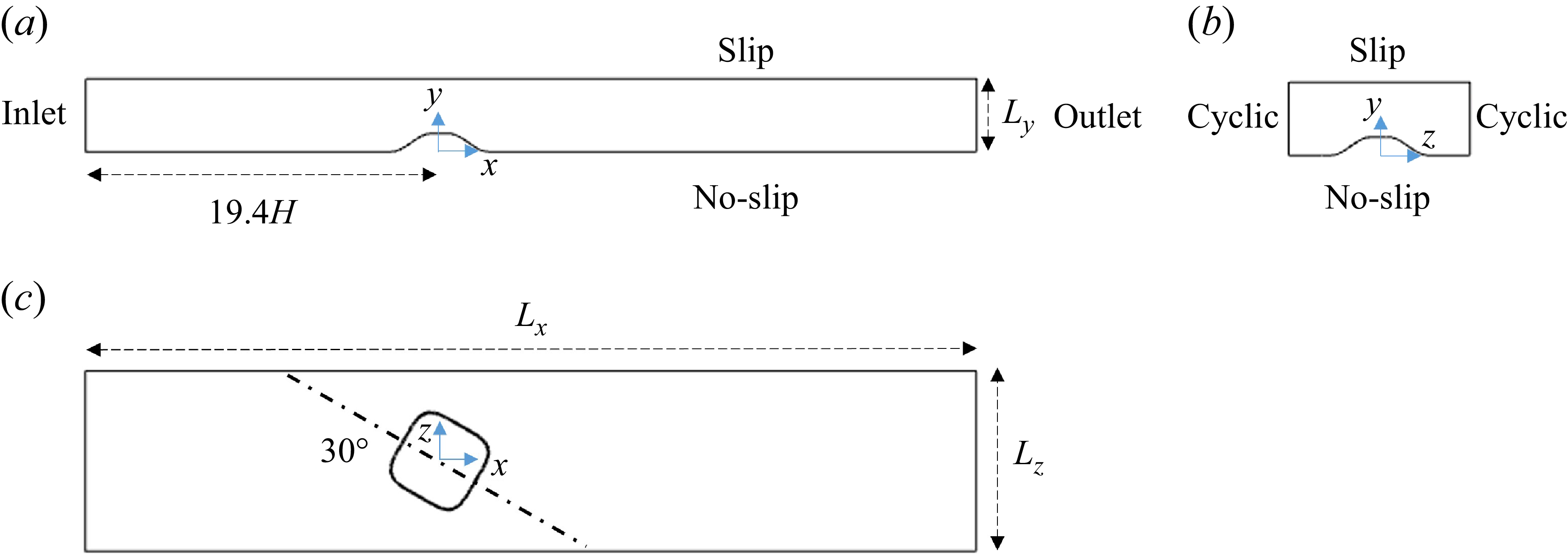


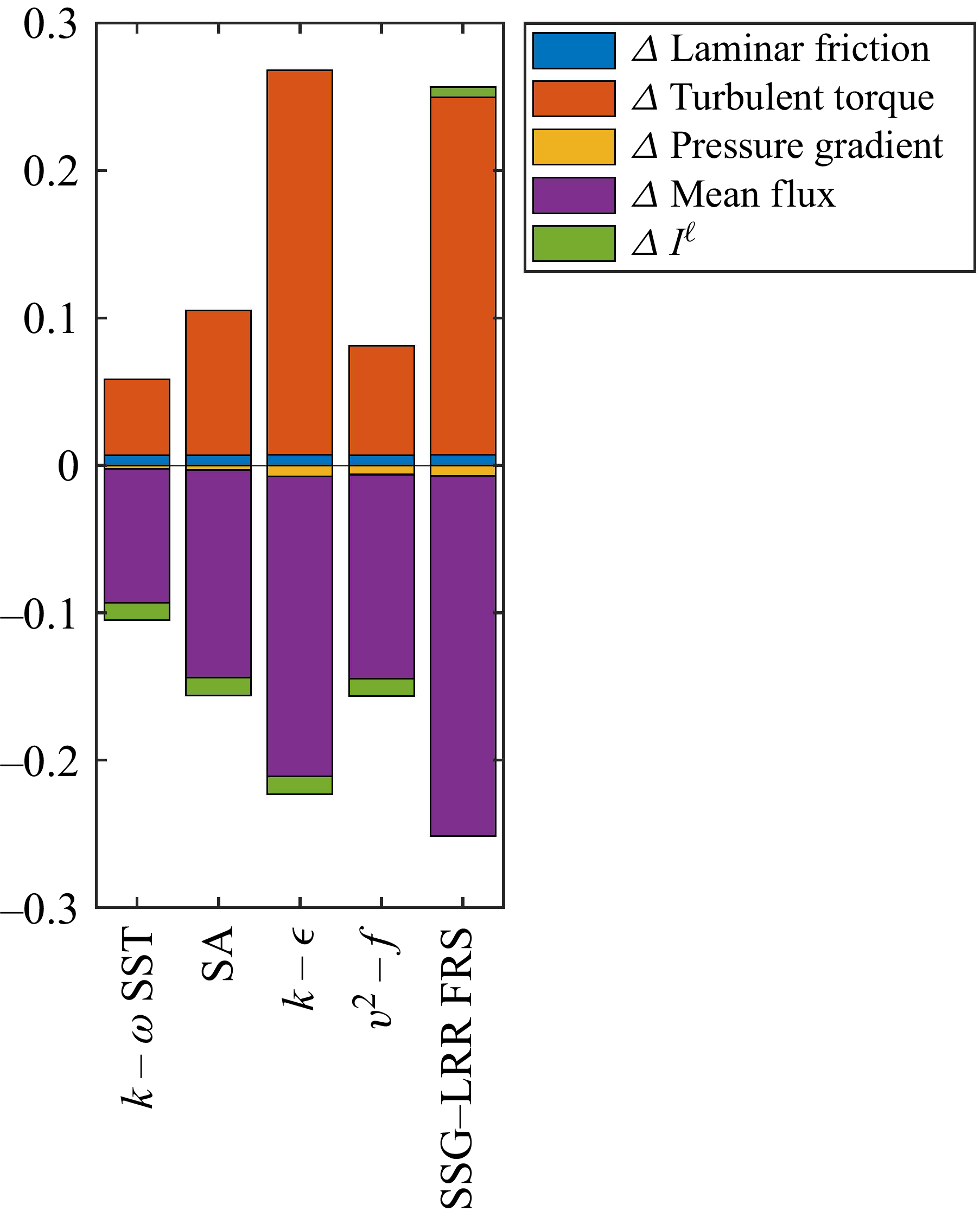


 Open access