


1. Introduction
The Ekman layer is a boundary layer where the Coriolis force balances the action of viscosity normal to the boundary (Ekman Reference Ekman1905; Pedlosky Reference Pedlosky1987; Vallis Reference Vallis2017a ). First discovered at the ocean surface, Ekman layers appear in a wide variety of settings. At their outer edge, away from the boundary, Ekman layers can induce flow in the direction normal to the boundary; these flows are called Ekman pumping or suction. Ekman pumping is fundamental to our understanding of ocean circulation. In simple models of the ocean circulation, Ekman layers mediate the transfer of momentum from the atmosphere to the ocean, and their associated pumping drives overturning cells (Price, Weller & Schudlich Reference Price, Weller and Schudlich1987; Vallis Reference Vallis2017c ). The Ekman layer can also be used to model the eventual transfer of momentum from the ocean to the Earth at the ocean floor: viscous dissipation in the bottom boundary layer could account for at least 25 % of the total power input to large-scale ocean eddies, i.e. 0.2 TW (Sen, Scott & Arbic Reference Sen, Scott and Arbic2008; Ferrari & Wunsch Reference Ferrari and Wunsch2009).
The alignment of thermal anomalies with Ekman pumping’s volume transport can drastically alter the heat flux in convectively driven rotating turbulence (Plumley et al. Reference Plumley, Julien, Marti and Stellmach2016, Reference Plumley, Julien, Marti and Stellmach2017; Tro, Grooms & Julien Reference Tro, Grooms and Julien2025). This paper demonstrates that a similar effect can occur in stably stratified quasi-geostrophic (QG) flow: the alignment of buoyancy anomalies with Ekman pumping’s volume transport can induce a net vertical buoyancy flux. We focus on the bottom boundary, where the lateral flow transitions from its value in the interior of the fluid to zero at the boundary across a frictional Ekman layer. Near the bottom boundary, but outside the Ekman layer, the Ekman-induced vertical buoyancy flux slightly weakens the local stratification. Diabatic mixing driven by any one of a wide range of processes, including wave breaking and overturning convection, can similarly weaken stratification; the effect is notable here for being the result of an adiabatic process. Without Ekman pumping, we show that the vertical buoyancy flux results in a slight strengthening of the stratification, and that Ekman pumping enhances this effect away from the boundary. In addition to altering the stratification, the Ekman-induced vertical buoyancy flux is associated with conversions between eddy available potential energy and eddy kinetic energy.
We opt here to study the freely decaying scenario. It is far more common to study QG turbulence in a statistically steady state driven by the baroclinic instability of an imposed vertically sheared horizontal flow, whose shear is in thermal–wind balance with a mean lateral buoyancy gradient. In such a scenario, it is well known that the eddy dynamics drives an overturning circulation with a non-zero vertical buoyancy flux; recent results on the vertical buoyancy flux in this setting have been derived by Gallet et al. (Reference Gallet, Miquel, Hadjerci, Burns, Flierl and Ferrari2022) and Meunier, Miquel & Gallet (Reference Meunier, Miquel and Gallet2023). We study the freely decaying case to emphasise that the Ekman-driven vertical buoyancy flux is active even in the absence of a mean lateral buoyancy gradient.
Section 2 provides a theoretical description of this buoyancy flux and its effects. Numerical experiments are described in § 3, and their results are presented in § 4. Conclusions are offered in § 5.
2. Ekman-driven buoyancy flux at the bottom boundary
2.1. The QG model
We frame our investigation in the context of the continuously-stratified QG model (Vallis Reference Vallis2017b ). The QG model’s dynamics is governed by conservation of QG potential vorticity (PV):
 \begin{align} \partial _{t}q + J[\psi ,q] = 0. \end{align}
Here, $q$
is the QGPV,
$q$
is the QGPV, $\psi$
is a streamfunction for lateral velocity
$\psi$
is a streamfunction for lateral velocity $\partial _{x}\psi =v,\ \partial _{y}\psi =-u$
, and
$\partial _{x}\psi =v,\ \partial _{y}\psi =-u$
, and $J[\psi ,q] = \partial _{x}\psi\, \partial _{y}q - \partial _{x}q\partial _{y}\psi = \boldsymbol{u}\boldsymbol{\cdot }\boldsymbol{\nabla }q$
. The symbol
$J[\psi ,q] = \partial _{x}\psi\, \partial _{y}q - \partial _{x}q\partial _{y}\psi = \boldsymbol{u}\boldsymbol{\cdot }\boldsymbol{\nabla }q$
. The symbol $\boldsymbol{\nabla}$
here and throughout indicates the gradient with respect to the horizontal coordinates only:
$\boldsymbol{\nabla}$
here and throughout indicates the gradient with respect to the horizontal coordinates only: $\boldsymbol{\nabla }= (\partial _{x},\partial _{y})$
.
$\boldsymbol{\nabla }= (\partial _{x},\partial _{y})$
.
The streamfunction $\psi$
is obtained from the QGPV
$\psi$
is obtained from the QGPV $q$
as the solution of an elliptic problem of the form
$q$
as the solution of an elliptic problem of the form
 \begin{align} {\nabla} ^2\psi + \partial _{z}\left (\frac{f^2}{N^2(z)}\partial _{z}\psi \right ) = q, \end{align}
where $f$
is the local Coriolis parameter, and
$f$
is the local Coriolis parameter, and $N(z)$
is the buoyancy frequency. The buoyancy frequency is related to a background buoyancy profile
$N(z)$
is the buoyancy frequency. The buoyancy frequency is related to a background buoyancy profile $\bar {b}(z)$
via
$\bar {b}(z)$
via
 \begin{align} N^2(z) = \partial _{z}\bar {b}. \end{align}
In the QG approximation, hydrostatic balance is expressed as
 \begin{equation} f \partial _{z}\psi = b - \bar {b}. \end{equation}
This balance, evaluated at the top and bottom boundaries, provides boundary conditions on the QGPV inversion problem (2.2):
 \begin{align} f\partial _{z}\psi = b - \bar {b}\quad\text{at}\quad z = 0, H. \end{align}
The buoyancy anomaly $b_0$
at the bottom surface is itself obtained as the solution of
$b_0$
at the bottom surface is itself obtained as the solution of
 \begin{align} \partial _{t}b_0 + J[\psi _0,b_0] + w_0N_0^2 = 0, \end{align}
where $w_0$
is the Ekman pumping velocity, and the subscript
$w_0$
is the Ekman pumping velocity, and the subscript $0$
indicates evaluation at
$0$
indicates evaluation at $z=0$
. Equation (2.6) is, in fact, the QG buoyancy equation, which holds throughout the fluid, evaluated on the bottom boundary, and another copy of (2.6) is active at the top boundary. For simplicity of exposition, we assume that there is no Ekman layer at the top boundary, e.g. because there is no stress at that boundary, which sets the pumping velocity to zero at the top. The classical solution for the pumping velocity
$z=0$
. Equation (2.6) is, in fact, the QG buoyancy equation, which holds throughout the fluid, evaluated on the bottom boundary, and another copy of (2.6) is active at the top boundary. For simplicity of exposition, we assume that there is no Ekman layer at the top boundary, e.g. because there is no stress at that boundary, which sets the pumping velocity to zero at the top. The classical solution for the pumping velocity $w_0$
at the bottom boundary produced by a linear Ekman boundary layer is
$w_0$
at the bottom boundary produced by a linear Ekman boundary layer is
 \begin{align} w_0 = \frac{d_E}{2}\omega _0, \end{align}
where $d_E$
is the depth of the Ekman layer, and
$d_E$
is the depth of the Ekman layer, and $\omega _0 = {\nabla} ^2\psi _0$
is the vertical component of relative vorticity evaluated at
$\omega _0 = {\nabla} ^2\psi _0$
is the vertical component of relative vorticity evaluated at $z=0$
(Vallis Reference Vallis2017b
, Eq. 5.209). This expression for the velocity at the outer edge of the Ekman layer is obtained as an asymptotic approximation in the limit of small Ekman number
$z=0$
(Vallis Reference Vallis2017b
, Eq. 5.209). This expression for the velocity at the outer edge of the Ekman layer is obtained as an asymptotic approximation in the limit of small Ekman number $E = \nu _z/(f\! H^2)\ll 1$
, where
$E = \nu _z/(f\! H^2)\ll 1$
, where $\nu _z$
is the vertical viscosity coefficient. We formally consider this pumping velocity to apply at
$\nu _z$
is the vertical viscosity coefficient. We formally consider this pumping velocity to apply at $z=0$
, which is not exact, but is asymptotically accurate since the outer edge of the Ekman layer occurs at depth
$z=0$
, which is not exact, but is asymptotically accurate since the outer edge of the Ekman layer occurs at depth $d_E\sim \sqrt {E}H$
.
$d_E\sim \sqrt {E}H$
.
Classical QG theory assumes that $\bar {b}$
and hence
$\bar {b}$
and hence $N^2$
are functions only of
$N^2$
are functions only of $z$
, but this can be relaxed via multiple-scales asymptotics to allow slow, large-scale variations (Pedlosky Reference Pedlosky1984; Grooms, Julien & Fox-Kemper Reference Grooms, Julien and Fox-Kemper2011). For our purposes here, it is enough to consider slow variation in time, and to note that the slow evolution of
$z$
, but this can be relaxed via multiple-scales asymptotics to allow slow, large-scale variations (Pedlosky Reference Pedlosky1984; Grooms, Julien & Fox-Kemper Reference Grooms, Julien and Fox-Kemper2011). For our purposes here, it is enough to consider slow variation in time, and to note that the slow evolution of $\bar {b}$
is governed by
$\bar {b}$
is governed by
 \begin{align} \partial _{t}\bar {b} = -\partial _{z}\left (\overline {wb}\right )\!, \end{align}
where $w$
is the vertical component of velocity. This is a dimensional version of (91) from Grooms et al. (Reference Grooms, Julien and Fox-Kemper2011), ignoring lateral buoyancy fluxes and lateral variations of
$w$
is the vertical component of velocity. This is a dimensional version of (91) from Grooms et al. (Reference Grooms, Julien and Fox-Kemper2011), ignoring lateral buoyancy fluxes and lateral variations of $\bar {b}$
. This formula ignores any diabatic effects that might operate, and considers only the horizontally averaged vertical buoyancy flux
$\bar {b}$
. This formula ignores any diabatic effects that might operate, and considers only the horizontally averaged vertical buoyancy flux $\overline {wb}$
affected by the balanced flow. According to the asymptotic analysis of Grooms et al. (Reference Grooms, Julien and Fox-Kemper2011), the buoyancy flux associated with the QG dynamics is small, so that changes in
$\overline {wb}$
affected by the balanced flow. According to the asymptotic analysis of Grooms et al. (Reference Grooms, Julien and Fox-Kemper2011), the buoyancy flux associated with the QG dynamics is small, so that changes in $\bar {b}$
are of the order of the Rossby number squared or smaller. From another perspective, an order-one change in
$\bar {b}$
are of the order of the Rossby number squared or smaller. From another perspective, an order-one change in $\bar {b}$
requires a time on the order of at least one over the Rossby number squared to accumulate.
$\bar {b}$
requires a time on the order of at least one over the Rossby number squared to accumulate.
The vertical flux $\overline {wb}$
depends on the vertical velocity
$\overline {wb}$
depends on the vertical velocity $w$
, which has not yet been specified. It is given by the solution of the QG omega equation (Davies Reference Davies2015)
$w$
, which has not yet been specified. It is given by the solution of the QG omega equation (Davies Reference Davies2015)
 \begin{align} N^2(z){\nabla} ^2w + f^2\partial _{z}^2 w = f\partial _{z}\left (J[\psi ,\omega ]\right ) -f{\nabla} ^2\left (J[\psi ,\partial _{z}\psi ]\right )\!, \end{align}
supplemented by boundary conditions
 \begin{equation} w = w_0 \text{ at }z = 0,\quad w=0\text{ at }z=H, \end{equation}
where $w_0$
is given by (2.7). Ekman pumping at the top surface is allowed in principle, but omitted here for simplicity. As noted above, applying the pumping velocity at
$w_0$
is given by (2.7). Ekman pumping at the top surface is allowed in principle, but omitted here for simplicity. As noted above, applying the pumping velocity at $z=0$
is not exact: it is an asymptotic approximation, because the pumping velocity occurs at the top of the Ekman layer.
$z=0$
is not exact: it is an asymptotic approximation, because the pumping velocity occurs at the top of the Ekman layer.
It will be useful to express $w$
as the sum of a part associated with the Ekman pumping
$w$
as the sum of a part associated with the Ekman pumping $w^E$
, and a part associated with the interior dynamics
$w^E$
, and a part associated with the interior dynamics $w^I$
. To wit, let
$w^I$
. To wit, let
 \begin{equation} w = w^E + w^I, \end{equation}
where
 \begin{align} N^2(z){\nabla} ^2w^E + f^2\partial _{z}^2 w^E = 0, \end{align}
supplemented by boundary conditions
 \begin{equation} w^E = w_0 \text{ at }z = 0,\quad w^E=0\text{ at }z=H. \end{equation}
The vertical velocity associated with Ekman pumping clearly does not end at the top of the Ekman layer, but rather extends into the fluid interior.
2.2. Vertical buoyancy flux and energetics
This subsection briefly reviews the connection between the vertical buoyancy flux and energetics. When there is no Ekman layer ( $w_0=0$
), the QG model of the previous subsection conserves the sum of kinetic energy (KE) and QG eddy available potential energy (APE)
$w_0=0$
), the QG model of the previous subsection conserves the sum of kinetic energy (KE) and QG eddy available potential energy (APE)
 \begin{align} {E}_{\textit{QG}} &= {\textit{KE}} + {\textit{APE}}, \end{align}
 \begin{align} {\textit{KE}} &= \frac{1}{2H}\int \overline {|\boldsymbol{\nabla }\psi |^2}\,{\textrm{d}}z = \frac{1}{2H}\int \overline {|\boldsymbol{u}|^2}\,{\textrm{d}}z ,\end{align}
 \begin{align} {\textit{APE}} &= \frac{1}{2H}\int _0^H \frac{\overline {b^2}}{N^2(z)}\,{\textrm{d}}z, \end{align}
 \begin{align} \frac{{\textrm{d}}{\textit{KE}}}{{\textrm{d}}t} &= \frac{1}{H}\int _0^H \overline {wb}\,{\textrm{d}}z, \end{align}
 \begin{align} \frac{{\textrm{d}}{\textit APE}}{{\textrm{d}}t} &= -\frac{{\textrm{d}}{\textit{KE}}}{{\textrm{d}}t}. \end{align}
The overbar $\overline {({\cdot })}$
represents an average over the horizontal extent of the domain. The KE and APE are normalised to represent energies per unit mass, with dimensions of length squared over time squared. The depth-integrated vertical buoyancy flux accounts for conversions between KE and APE; linear and nonlinear baroclinic instability, for example, convert APE to KE via the vertical buoyancy flux.
$\overline {({\cdot })}$
represents an average over the horizontal extent of the domain. The KE and APE are normalised to represent energies per unit mass, with dimensions of length squared over time squared. The depth-integrated vertical buoyancy flux accounts for conversions between KE and APE; linear and nonlinear baroclinic instability, for example, convert APE to KE via the vertical buoyancy flux.
The Ekman layer removes KE, as is well known. We point out here that the vertical buoyancy flux associated with the Ekman layer also induces conversions between KE and APE. To see this, we use the QG vorticity equation
 \begin{equation} \partial _{t}\omega + J[\psi ,\omega ] - f\partial _{z}w = 0. \end{equation}
The evolution of KE is derived by multiplying the vorticity equation by $-\psi$
and averaging over the volume, using several integrations by parts. The advective term conserves KE, so we focus on the planetary vortex stretching term
$-\psi$
and averaging over the volume, using several integrations by parts. The advective term conserves KE, so we focus on the planetary vortex stretching term $-f\partial _{z}w$
. The KE tendency is
$-f\partial _{z}w$
. The KE tendency is
 \begin{equation} \frac{{\textrm{d}}{\textit{KE}}}{{\textrm{d}}t} = -\frac{f}{H}\int _0^H\overline {\psi\, \partial _{z}w}\,{\textrm{d}}z. \end{equation}
A single integration by parts in the vertical direction using the boundary conditions on $w$
and the QG hydrostatic balance (2.4) yields
$w$
and the QG hydrostatic balance (2.4) yields
 \begin{equation} \frac{{\textrm{d}}{\textit{KE}}}{{\textrm{d}}t} = \frac{f}{H}\,\overline {\psi _0 w_0} + \frac{1}{H}\int _0^H\overline {wb}\,{\textrm{d}}z. \end{equation}
Using the linear Ekman velocity (2.7) and an integration by parts in the horizontal yields
 \begin{equation} \frac{{\textrm{d}}{\textit{KE}}}{{\textrm{d}}t} = -\frac{fd_E}{2H}\,\overline {|\boldsymbol{u}_0|^2} + \frac{1}{H}\int _0^H\overline {wb}\,{\textrm{d}}z. \end{equation}
The Ekman layer clearly leads to dissipation of KE via the first term on the right-hand side.
Per the discussion in the previous subsection, we note that there is a component $w^E$
of
$w^E$
of $w$
that comes from Ekman pumping and extends into the interior of the fluid, above the top of the Ekman layer. The conversion term in the KE equation can thus be expanded, yielding
$w$
that comes from Ekman pumping and extends into the interior of the fluid, above the top of the Ekman layer. The conversion term in the KE equation can thus be expanded, yielding
 \begin{equation} \frac{{\textrm{d}}{\textit{KE}}}{{\textrm{d}}t} = -\frac{fd_E}{2H}\,\overline {|\boldsymbol{u}_0|^2} + \frac{1}{H}\int _0^H\overline {w^Eb}\,{\textrm{d}}z + \frac{1}{H}\int _0^H\overline {w^Ib}\,{\textrm{d}}z. \end{equation}
As we will see in the following two subsections, the vertical velocity associated with Ekman pumping can lead to conversions between KE and APE in a process distinct from baroclinic instability.
The mean gravitational potential energy of the fluid is proportional to
 \begin{equation} {\textit{MPE}} = \frac{1}{H}\int _0^H -z\bar {b}\,{\textrm{d}}z. \end{equation}
The evolution of MPE can be obtained from (2.8) by multiplying by $z$
and averaging across depth. One integration by parts yields
$z$
and averaging across depth. One integration by parts yields
 \begin{equation} \frac{{\textrm{d}}{\textit{MPE}}}{{\textrm{d}}t} = -\frac{1}{H}\int _0^H\overline {wb}\,{\textrm{d}}z. \end{equation}
The tendencies of QG APE and of MPE are the same. Any conversion of QG APE into KE is thus also necessarily associated with a reduction of MPE, and the associated change in $\bar {b}$
is accomplished by the divergence of the vertical buoyancy flux acting in (2.8).
$\bar {b}$
is accomplished by the divergence of the vertical buoyancy flux acting in (2.8).
2.3. Surface QG vertical buoyancy flux
We obtain insight into the vertical buoyancy flux near the bottom boundary by considering the surface QG (sQG) model (Held et al. Reference Held, Pierrehumbert, Garner and Swanson1995; Lapeyre Reference Lapeyre2017). This model is obtained from the full QG model by setting $q=0$
and considering horizontal scales much smaller than the first baroclinic deformation radius, which is approximately
$q=0$
and considering horizontal scales much smaller than the first baroclinic deformation radius, which is approximately $(f\unicode{x03C0} )^{-1}\int _0^HN(z){\textrm{d}}z$
(Robey & Grooms Reference Robey and Grooms2024). The result is a model whose dynamics is entirely controlled by surface buoyancy
$(f\unicode{x03C0} )^{-1}\int _0^HN(z){\textrm{d}}z$
(Robey & Grooms Reference Robey and Grooms2024). The result is a model whose dynamics is entirely controlled by surface buoyancy
 \begin{align} \partial _{t}b_0 + J[\psi _0,b_0] + \frac{d_EN_0^2}{2}\omega _0 = 0, \end{align}
where the assumptions imply that $\psi _0$
is, to leading order, independent of
$\psi _0$
is, to leading order, independent of $b$
at the top boundary. The sQG model is often simplified by assuming that
$b$
at the top boundary. The sQG model is often simplified by assuming that $N^2(z)$
is depth-independent, though this is not necessary, and depth dependence of
$N^2(z)$
is depth-independent, though this is not necessary, and depth dependence of $N^2(z)$
can have important effects (Yassin & Griffies Reference Yassin and Griffies2022). Nonetheless, for simplicity of exposition, we make the same assumption here, that
$N^2(z)$
can have important effects (Yassin & Griffies Reference Yassin and Griffies2022). Nonetheless, for simplicity of exposition, we make the same assumption here, that $N^2(z) = N_0^2$
. This assumption is relaxed in § A.1, where we show similar behaviour in a stretched vertical coordinate.
$N^2(z) = N_0^2$
. This assumption is relaxed in § A.1, where we show similar behaviour in a stretched vertical coordinate.
With this assumption, the classical sQG theory relates $b_0$
and
$b_0$
and $\psi _0$
via the fractional Laplacian
$\psi _0$
via the fractional Laplacian
 \begin{align} \psi _0 = -\frac{1}{N_0}\big(-{\nabla} ^2\big)^{-1/2}b_0. \end{align}
The Ekman pumping velocity is therefore
 \begin{align} w_0 = \frac{d_E}{2}{\nabla} ^2\psi _0 = \frac{d_E}{2N_0}\big(-{\nabla} ^2\big)^{1/2}b_0, \end{align}
and the vertical buoyancy flux at the bottom is
 \begin{equation} \overline {w_0b_0} = \frac{d_E}{2N_0}\overline {\left |\left (-{\nabla} ^2\right )^{1/4}b_0\right |^2}\gt 0. \end{equation}
The sign here is important because it implies that Ekman pumping reduces buoyancy variance at the bottom boundary.
The effect of the vertical buoyancy flux on the background stratification requires knowledge of its vertical profile, not merely its value at the bottom of the layer. To gain insight, we move to the Fourier domain, and explore how $b$
and
$b$
and $w$
transition from their boundary values towards the interior of the domain. Plancherel’s identity relates the vertical buoyancy flux to the Fourier transforms of
$w$
transition from their boundary values towards the interior of the domain. Plancherel’s identity relates the vertical buoyancy flux to the Fourier transforms of $w$
and
$w$
and $b$
:
$b$
:
 \begin{equation} \overline {wb} = \int \hat {w}_k(z)\hat {b}_k^*(z){\textrm{d}}\boldsymbol{k}, \end{equation}
where $^*$
indicates complex conjugation, and
$^*$
indicates complex conjugation, and $\boldsymbol{k}=(k_x,k_y)$
is the lateral wavenumber. This expresses the total vertical buoyancy flux as an integral over vertical fluxes coming from different wavenumbers, and hence from different horizontal length scales.
$\boldsymbol{k}=(k_x,k_y)$
is the lateral wavenumber. This expresses the total vertical buoyancy flux as an integral over vertical fluxes coming from different wavenumbers, and hence from different horizontal length scales.
At fixed $z$
, the quantity
$z$
, the quantity $\hat {w}_k(z)\hat {b}_k^*(z)$
is a two-dimensional co-spectrum. The one-dimensional co-spectrum, which is a function only of the wavenumber magnitude
$\hat {w}_k(z)\hat {b}_k^*(z)$
is a two-dimensional co-spectrum. The one-dimensional co-spectrum, which is a function only of the wavenumber magnitude $k = \sqrt {k_x^2+k_y^2}$
, is found by changing to polar coordinates in the integral, which yields
$k = \sqrt {k_x^2+k_y^2}$
, is found by changing to polar coordinates in the integral, which yields
 \begin{equation} \overline {wb} = \int _0^\infty \left [k\int _0^{2\unicode{x03C0} }\hat {w}_k(z)\hat {b}_k^*(z){\textrm{d}}\theta \right ]{\textrm{d}}k, \end{equation}
where the quantity in square brackets is the one-dimensional co-spectrum of $w$
and
$w$
and $b$
.
$b$
.
The Fourier transform $\hat {\psi }_k$
of the streamfunction
$\hat {\psi }_k$
of the streamfunction $\psi$
is obtained as the solution of the boundary value problem
$\psi$
is obtained as the solution of the boundary value problem
 \begin{equation} -k^2\,\hat {\psi }_k(z) + \frac{f^2}{N_0^2}\,\hat {\psi }_k^{\prime \prime}(z) = 0, \quad 0\lt z\lt \infty , \end{equation}
with boundary conditions
 \begin{align} f\,\hat {\psi }_k^{\prime}(z=0) = \hat {b}_k(z=0),\quad\lim _{z\to \infty }\hat {\psi }_k(z) = 0. \end{align}
(The switch to a semi-infinite domain here is justified a posteriori by the fact that the effect of the top boundary condition on the solution near the bottom boundary is beyond-all-orders under the sQG assumption of horizontal scales much smaller than the first baroclinic deformation radius.) The solution is
 \begin{equation} \hat {\psi }_k(z) = -\frac{\hat {b}_k(z=0)}{kN_0}\,{\textrm{e}}^{-\frac{kN_0}{f}z}, \end{equation}
which incidentally explains (2.23). Hydrostatic balance (2.4) and (2.30) together imply that $\hat {b}_k$
decays exponentially into the interior of the fluid:
$\hat {b}_k$
decays exponentially into the interior of the fluid:
 \begin{equation} \hat {b}_k(z) = \hat {b}_k(z=0)\,{\textrm{e}}^{-\frac{kN_0}{f}z}. \end{equation}
To understand how $w$
changes from its boundary value
$w$
changes from its boundary value $w_0$
towards the interior of the fluid, we return to the QG omega equation (2.9). The interior component
$w_0$
towards the interior of the fluid, we return to the QG omega equation (2.9). The interior component $w^I$
of the vertical velocity does not admit a simple analysis. In contrast, the Ekman component of the vertical velocity can be solved for exactly, which yields
$w^I$
of the vertical velocity does not admit a simple analysis. In contrast, the Ekman component of the vertical velocity can be solved for exactly, which yields
 \begin{align} \hat {w}_k^E(z) = \hat {w}_k^E(z=0)\,{\textrm{e}}^{-\frac{kN_0}{f}z} = \frac{d_Ek}{2N_0}\,\hat {b}_k(z=0)\,{\textrm{e}}^{-\frac{kN_0}{f}z}. \end{align}
Plancherel’s identity for the sQG vertical buoyancy flux becomes
 \begin{equation} \overline {wb} = \overline {w^Ib} + \frac{d_E}{2N_0}\int k\,|\hat {b}_k(z=0)|^2\,{\textrm{e}}^{-2\frac{kN_0}{f}z}\,{\textrm{d}}\boldsymbol{k}. \end{equation}
The last term in the expression above results directly from Ekman pumping. Its positive sign implies that near the bottom, the effect of Ekman pumping is to convert APE to KE. This conversion has the same sign as in linear baroclinic instability, but is affected by a completely different process. It also partially offsets the direct action of Ekman friction to remove KE.
Per (2.8), the tendency of $\bar {b}$
equals minus the divergence of this flux, which is
$\bar {b}$
equals minus the divergence of this flux, which is
 \begin{equation} \partial _{t}\bar {b} = -\partial _{z}\big(\overline {w^Ib}\big) + \frac{d_E}{f}\int k^2\,|\hat {b}_k(z=0)|^2\,{\textrm{e}}^{-2\frac{kN_0}{f}z}\,{\textrm{d}}\boldsymbol{k}. \end{equation}
The last term comes directly from Ekman pumping. It is positive and decays towards the interior. In a stably stratified fluid, $\bar {b}$
is an increasing function of depth, so a positive tendency near the bottom tends to weaken the stratification. This tendency to weaken the stratification is qualitatively similar to the effect of diabatic mixing, but the effect is accomplished here by an adiabatic process.
$\bar {b}$
is an increasing function of depth, so a positive tendency near the bottom tends to weaken the stratification. This tendency to weaken the stratification is qualitatively similar to the effect of diabatic mixing, but the effect is accomplished here by an adiabatic process.
The first term, associated with $w^I$
, is harder to analyse. Using an sQG model without an Ekman layer, Capet et al. (Reference Capet, Klein, Hua, Lapeyre and Mcwilliams2008) found that the vertical buoyancy flux is positive in the interior of the fluid, and also tends to convert APE to KE. In our numerical experiments described below, the interior term is smaller than the Ekman term near the boundary, so that the total effect is to weaken the stratification near the bottom boundary.
$w^I$
, is harder to analyse. Using an sQG model without an Ekman layer, Capet et al. (Reference Capet, Klein, Hua, Lapeyre and Mcwilliams2008) found that the vertical buoyancy flux is positive in the interior of the fluid, and also tends to convert APE to KE. In our numerical experiments described below, the interior term is smaller than the Ekman term near the boundary, so that the total effect is to weaken the stratification near the bottom boundary.
2.4. Ekman-induced vertical buoyancy flux at large horizontal scales
The sQG analysis in the previous subsection is appropriate only near the bottom boundary, and at horizontal scales smaller than the deformation radius. The Ekman-driven vertical buoyancy flux from the previous subsection should therefore be thought of as only part of the total Ekman-driven buoyancy flux, the part coming from scales smaller than the deformation radius. At very large horizontal scales, the dual-cascade theory of QG turbulence suggests that the flow is approximately barotropic (depth-independent) (Salmon Reference Salmon1978; Larichev & Held Reference Larichev and Held1995; Smith & Vallis Reference Smith and Vallis2001).
To develop a heuristic for the sign of the Ekman-driven buoyancy flux at large scales, consider the surface buoyancy equation (2.6). The net buoyancy variance at the bottom boundary evolves according to
 \begin{equation} \frac{1}{2}\frac{{\textrm{d}}}{{\textrm{d}}t}\overline {b_0^2} = -\overline {w_0b_0}\,N_0^2. \end{equation}
The Ekman pumping velocity $w_0$
is driven by the bottom vorticity via (2.7), but unlike the sQG model, the bottom vorticity in this scenario comes mainly from the barotropic part of the flow, which is not directly related to the buoyancy at the bottom
$w_0$
is driven by the bottom vorticity via (2.7), but unlike the sQG model, the bottom vorticity in this scenario comes mainly from the barotropic part of the flow, which is not directly related to the buoyancy at the bottom $b_0$
. So we can think of the Ekman pumping velocity
$b_0$
. So we can think of the Ekman pumping velocity $w_0$
as driving large-scale buoyancy anomalies, of which it is largely independent. Heuristically, we expect this type of process to increase buoyancy variance at the bottom, i.e. for
$w_0$
as driving large-scale buoyancy anomalies, of which it is largely independent. Heuristically, we expect this type of process to increase buoyancy variance at the bottom, i.e. for $\overline {w_0b_0}$
to be negative. This is the opposite sign from the sQG model of the previous subsection.
$\overline {w_0b_0}$
to be negative. This is the opposite sign from the sQG model of the previous subsection.
As in the previous subsection, we are interested not only in $\overline {wb}$
at the bottom, but also in its progression towards the fluid interior. While the analysis of the previous subsection still applies to
$\overline {wb}$
at the bottom, but also in its progression towards the fluid interior. While the analysis of the previous subsection still applies to $w^E$
(namely that it decays from its boundary value toward the interior), lacking the simplifying sQG assumptions, we are unable to offer a kinematic prediction for how buoyancy
$w^E$
(namely that it decays from its boundary value toward the interior), lacking the simplifying sQG assumptions, we are unable to offer a kinematic prediction for how buoyancy $b$
changes from its boundary value towards the interior at large horizontal scales. In general, we can only conclude that the decay of
$b$
changes from its boundary value towards the interior at large horizontal scales. In general, we can only conclude that the decay of $w^E$
from its boundary value towards the interior will be slower at large scales than at small scales.
$w^E$
from its boundary value towards the interior will be slower at large scales than at small scales.
3. Experimental configuration
To study the vertical buoyancy flux in QG dynamics, we run freely decaying simulations in a horizontally periodic domain of width 2048 km and depth 5.2 km. The Coriolis parameter is $f=10^{-4}$
s
$f=10^{-4}$
s $^{-1}$
. We run six simulations: two different stratification profiles, and three different Ekman layer depths (including zero, i.e. stress-free). Half the simulations use a constant value
$^{-1}$
. We run six simulations: two different stratification profiles, and three different Ekman layer depths (including zero, i.e. stress-free). Half the simulations use a constant value $N = 19.33f$
, which leads to deformation radius
$N = 19.33f$
, which leads to deformation radius $NH/(f\unicode{x03C0} ) = 32$
km, while the other half use the following expression for
$NH/(f\unicode{x03C0} ) = 32$
km, while the other half use the following expression for $N(z)$
:
$N(z)$
:
 \begin{equation} N(z) = f \left [c_0 + c_1 \frac{z}{H} + \frac{c_2 w}{\unicode{x03C0} ((z/H-z_0)^2+w^2)}\right ] \end{equation}
with $c_0= 6.3$
,
$c_0= 6.3$
, $c_1=22$
,
$c_1=22$
, $c_2 = 4.5$
,
$c_2 = 4.5$
, $w=0.03$
and
$w=0.03$
and $z_0 = 0.97$
. This follows Robey & Grooms (Reference Robey and Grooms2024) with some slight modifications in the parameter values; the profile is shown in figure 1. It qualitatively represents a main pycnocline near the top, underneath a more weakly stratified surface layer, and surmounting a weakly stratified abyss. The discrete deformation radius for this profile is also 32 km. For each stratification, we run one simulation without Ekman friction, and two simulations with Ekman friction. The two simulations with Ekman friction use Ekman layer depths of either
$z_0 = 0.97$
. This follows Robey & Grooms (Reference Robey and Grooms2024) with some slight modifications in the parameter values; the profile is shown in figure 1. It qualitatively represents a main pycnocline near the top, underneath a more weakly stratified surface layer, and surmounting a weakly stratified abyss. The discrete deformation radius for this profile is also 32 km. For each stratification, we run one simulation without Ekman friction, and two simulations with Ekman friction. The two simulations with Ekman friction use Ekman layer depths of either $5.2$
m or
$5.2$
m or $52$
m, the former constituting weak drag, and the latter strong drag. The next section presents the results for strong drag; the results for weak drag are shown in the supplementary material. Any qualitative differences are mentioned in the context of the corresponding strong drag results in the next section.
$52$
m, the former constituting weak drag, and the latter strong drag. The next section presents the results for strong drag; the results for weak drag are shown in the supplementary material. Any qualitative differences are mentioned in the context of the corresponding strong drag results in the next section.
The realistic stratification profile $N(z)/f$
given by (3.1).
$N(z)/f$
given by (3.1).

Each simulation uses an initial condition of the form
 \begin{equation} q(x,y,z,t=0) = q_{\textit{scale}}\, \phi (z)\cos \left (\frac{2\unicode{x03C0} x}{L} + \frac{\unicode{x03C0} }{4}\sin ^2\left (\frac{2\unicode{x03C0} y}{L}\right )\right )\!, \end{equation}
where $\phi (z)$
is the first baroclinic mode (Rocha, Young & Grooms Reference Rocha, Young and Grooms2016) associated with the simulation’s stratification. The values of
$\phi (z)$
is the first baroclinic mode (Rocha, Young & Grooms Reference Rocha, Young and Grooms2016) associated with the simulation’s stratification. The values of $q_{\textit{scale}}$
are chosen to achieve initial volume-averaged total energy per unit mass 0.044 m
$q_{\textit{scale}}$
are chosen to achieve initial volume-averaged total energy per unit mass 0.044 m $^2$
s−
$^2$
s− $^2$
. Because the initial condition is on a large horizontal scale and has a first-baroclinic-mode vertical structure, the initial total energy is almost entirely in the form of APE. Linear instability quickly sets in and converts potential energy to KE, generating a turbulent state.
$^2$
. Because the initial condition is on a large horizontal scale and has a first-baroclinic-mode vertical structure, the initial total energy is almost entirely in the form of APE. Linear instability quickly sets in and converts potential energy to KE, generating a turbulent state.
Biharmonic lateral diffusion of QGPV is added to avoid accumulation of enstrophy at small scales:
 \begin{align} \partial _{t}q + J[\psi ,q] = -\nu _4{\nabla} ^4q. \end{align}
The biharmonic coefficient $\nu _4$
is set as the maximum of several nonlinear viscosities. The biharmonic QG-Leith coefficient
$\nu _4$
is set as the maximum of several nonlinear viscosities. The biharmonic QG-Leith coefficient $\nu _{{QL}}(z)$
for the forward cascade of potential enstrophy in the interior of the fluid is
$\nu _{{QL}}(z)$
for the forward cascade of potential enstrophy in the interior of the fluid is
 \begin{align} \nu _{\textit{QL}}(z) = \left (2.2\times \frac{8\text{ km}}{\unicode{x03C0} }\right )^6\left (\overline {({\nabla} ^2q)^2}\right )^{1/2}. \end{align}
The biharmonic QG-Leith coefficient $\nu _0$
for the forward cascade of surface PV
$\nu _0$
for the forward cascade of surface PV $b_0/f$
on the bottom boundary is
$b_0/f$
on the bottom boundary is
 \begin{align} \nu _{0} = \frac{1}{f}\left (2.2\times \frac{8\text{ km}}{\unicode{x03C0} }\right )^5\left (\overline {\left({\nabla} ^2b_0\right)^2}\right )^{1/2}, \end{align}
and the biharmonic QG-Leith coefficient $\nu _1$
for the forward cascade of surface PV
$\nu _1$
for the forward cascade of surface PV $b_1/f$
on the top boundary is defined similarly. The final coefficient
$b_1/f$
on the top boundary is defined similarly. The final coefficient $\nu _4$
is set to the max of these, since the use of different or depth-dependent coefficients would not guarantee dissipation of energy:
$\nu _4$
is set to the max of these, since the use of different or depth-dependent coefficients would not guarantee dissipation of energy:
 \begin{equation} \nu _4 = \max\Big\{\nu _0,\nu _1,\max _{z\in [0,1]}\nu _{{QL}}\Big\}. \end{equation}
All simulations use a Fourier spectral method with 384 $\times$
384 modes in the horizontal, dealiased using the
$\times$
384 modes in the horizontal, dealiased using the $2/3$
rule; the effective grid scale after dealiasing is 8 km. The vertical discretisation scheme is as described by Grooms & Nadeau (Reference Grooms and Nadeau2016), and the time discretisation uses the implicit–explicit scheme ARK4(3)6L[2]SA from Kennedy & Carpenter (Reference Kennedy and Carpenter2003). The time step is set adaptively. The simulations with depth-independent
$2/3$
rule; the effective grid scale after dealiasing is 8 km. The vertical discretisation scheme is as described by Grooms & Nadeau (Reference Grooms and Nadeau2016), and the time discretisation uses the implicit–explicit scheme ARK4(3)6L[2]SA from Kennedy & Carpenter (Reference Kennedy and Carpenter2003). The time step is set adaptively. The simulations with depth-independent $N^2$
use 32 layers, while the simulations with the realistic profile from (3.1) use 64 layers. The choice of vertical grid spacing is elaborated in Appendix A. The code used here has been made publicly available (Grooms Reference Grooms2025).
$N^2$
use 32 layers, while the simulations with the realistic profile from (3.1) use 64 layers. The choice of vertical grid spacing is elaborated in Appendix A. The code used here has been made publicly available (Grooms Reference Grooms2025).
4. Results
We present here the results from four of the six simulations described in § 3, i.e. with and without Ekman pumping, and with either the realistic stratification given in (3.1) or a constant stratification. Results with Ekman pumping are presented for the strong drag case with $d_E = 52$
m; the results for weak drag are qualitatively similar but weaker, and are shown in the supplementary material. A visualisation of the flow in the case with Ekman pumping and realistic stratification is shown in figure 2. The Ekman component of vertical velocity is only visible near the bottom because it is weak away from the bottom, while vorticity is only visible near the top because it is weak away from the top. The evolution of the KE is shown in figure 3, as a percentage of the initial total energy. All four simulations begin with an initial growth of KE. The simulations are initialised with mostly APE, and linear baroclinic instability quickly converts this to KE. In the stress-free (without Ekman pumping) simulations, shown in figure 3(a), this conversion process continues until energy is almost entirely KE. The stress-free simulations lose a small amount of their total energy over the run due to the biharmonic diffusion of QGPV: the constant
$d_E = 52$
m; the results for weak drag are qualitatively similar but weaker, and are shown in the supplementary material. A visualisation of the flow in the case with Ekman pumping and realistic stratification is shown in figure 2. The Ekman component of vertical velocity is only visible near the bottom because it is weak away from the bottom, while vorticity is only visible near the top because it is weak away from the top. The evolution of the KE is shown in figure 3, as a percentage of the initial total energy. All four simulations begin with an initial growth of KE. The simulations are initialised with mostly APE, and linear baroclinic instability quickly converts this to KE. In the stress-free (without Ekman pumping) simulations, shown in figure 3(a), this conversion process continues until energy is almost entirely KE. The stress-free simulations lose a small amount of their total energy over the run due to the biharmonic diffusion of QGPV: the constant $N^2$
simulation loses 5 %, and the simulation with realistic stratification loses 8 %. In the simulations with Ekman pumping, KE peaks at approximately 25 % before the Ekman drag reduces it again.
$N^2$
simulation loses 5 %, and the simulation with realistic stratification loses 8 %. In the simulations with Ekman pumping, KE peaks at approximately 25 % before the Ekman drag reduces it again.
A snapshot of the simulation with realistic stratification and strong drag at $t=350$
days. The green and purple colours near the top show relative vorticity
$t=350$
days. The green and purple colours near the top show relative vorticity $\omega = {\nabla} ^2\psi$
, while the blue and red colours near the bottom show the Ekman component of the vertical velocity
$\omega = {\nabla} ^2\psi$
, while the blue and red colours near the bottom show the Ekman component of the vertical velocity $w^E$
. The opacity of each field is linked to its magnitude. Vertical velocity is only visible near the bottom because it is weak away from the bottom, while vorticity is only visible near the top because it is weak away from the top. Visualisation created using Vapor (Li et al. Reference Li, Jaroszynski, Pearse, Orf and Clyne2019; sgpearse et al. Reference Sgpearse, Li, StasJ, Daves, Hallock, Eroglu, Poplawski and Lacroix2023).
$w^E$
. The opacity of each field is linked to its magnitude. Vertical velocity is only visible near the bottom because it is weak away from the bottom, while vorticity is only visible near the top because it is weak away from the top. Visualisation created using Vapor (Li et al. Reference Li, Jaroszynski, Pearse, Orf and Clyne2019; sgpearse et al. Reference Sgpearse, Li, StasJ, Daves, Hallock, Eroglu, Poplawski and Lacroix2023).

Evolution through time of KE as a percentage of the total initial energy: (a) the stress-free simulations, and (b) the two simulations with Ekman pumping. The blue curves correspond to the simulations run with a constant stratification, and the orange curves correspond to the more realistic stratification (3.1).

In figure 4, we plot the vertical profiles of $\overline {wb}$
with Ekman pumping. The blue curve shows the sum of both components of
$\overline {wb}$
with Ekman pumping. The blue curve shows the sum of both components of $\overline {wb}$
, that is,
$\overline {wb}$
, that is, $\overline { (w^E+w^I )b}$
, and the orange dashed curve shows just the part from the Ekman component. At early times, the flow is large-scale, and the negative sign of
$\overline { (w^E+w^I )b}$
, and the orange dashed curve shows just the part from the Ekman component. At early times, the flow is large-scale, and the negative sign of $\overline {w^Eb}$
at the bottom is consistent with the heuristic argument in § 2.4. At later times, when there is more energy at small scales, we see that
$\overline {w^Eb}$
at the bottom is consistent with the heuristic argument in § 2.4. At later times, when there is more energy at small scales, we see that $\overline {w^Eb}$
becomes positive at the bottom, which again is consistent with the sQG argument for small scales in § 2.3. The results with weaker drag, shown in the supplementary material, are qualitatively similar but have a smaller Ekman component
$\overline {w^Eb}$
becomes positive at the bottom, which again is consistent with the sQG argument for small scales in § 2.3. The results with weaker drag, shown in the supplementary material, are qualitatively similar but have a smaller Ekman component $\overline {w^Eb}$
. At later times in the weak drag simulations, the Ekman component of the buoyancy flux remains negative throughout the volume of fluid; the sQG behaviour at small scales near the bottom is not strong enough to change the overall sign to positive, as it does in the strong drag case shown here.
$\overline {w^Eb}$
. At later times in the weak drag simulations, the Ekman component of the buoyancy flux remains negative throughout the volume of fluid; the sQG behaviour at small scales near the bottom is not strong enough to change the overall sign to positive, as it does in the strong drag case shown here.
Profiles of $\overline {wb}$
, time-averaged over various sections of the run time: (a) the simulation with constant stratification, and (b) the realistic stratification. The solid blue curves correspond to the sum of both components of
$\overline {wb}$
, time-averaged over various sections of the run time: (a) the simulation with constant stratification, and (b) the realistic stratification. The solid blue curves correspond to the sum of both components of $w$
,
$w$
, $w = w^E+w^I$
, and the dashed curves correspond to each component.
$w = w^E+w^I$
, and the dashed curves correspond to each component.

In figure 5, we plot the co-spectra of $b$
with
$b$
with $w$
, according to the quantity in brackets on the right-hand side of (2.27). This quantity is plotted in the
$w$
, according to the quantity in brackets on the right-hand side of (2.27). This quantity is plotted in the $k$
–
$k$
– $z$
plane and time-averaged over various sections of the run time. In the initial growth stage (approximately 0–50 days),
$z$
plane and time-averaged over various sections of the run time. In the initial growth stage (approximately 0–50 days), $\overline {wb}$
is positive and primarily large-scale, corresponding to a transfer of energy from APE to KE. In the middle section of run time, from
$\overline {wb}$
is positive and primarily large-scale, corresponding to a transfer of energy from APE to KE. In the middle section of run time, from $t = 50$
days until approximately the peak of KE,
$t = 50$
days until approximately the peak of KE, $\overline {wb}$
switches to a negative sign and reaches smaller scales, though still at least a factor of two larger than the deformation scale. In the time after the peak in KE, the rightmost panels in figure 5 show that
$\overline {wb}$
switches to a negative sign and reaches smaller scales, though still at least a factor of two larger than the deformation scale. In the time after the peak in KE, the rightmost panels in figure 5 show that $\overline {wb}$
becomes positive at scales smaller than approximately twice the deformation scale. The switch to negative sign at large scales is supported by the heuristic argument in § 2.4, and the positive values at small scales are supported by the sQG argument in § 2.3. In the weak drag simulations, the co-spectrum at intermediate times remains mostly positive away from the bottom boundary, even at the larger scales. Away from the bottom boundary, the co-spectrum is dominated by the interior component, which is positive.
$\overline {wb}$
becomes positive at scales smaller than approximately twice the deformation scale. The switch to negative sign at large scales is supported by the heuristic argument in § 2.4, and the positive values at small scales are supported by the sQG argument in § 2.3. In the weak drag simulations, the co-spectrum at intermediate times remains mostly positive away from the bottom boundary, even at the larger scales. Away from the bottom boundary, the co-spectrum is dominated by the interior component, which is positive.
Cospectra of $b$
with
$b$
with $w$
for the simulations with Ekman pumping, time-averaged over various sections of the run time: (a) the simulation with a constant stratification, and (b) the realistic stratification. All are horizontal co-spectra plotted as a function of depth, in accordance with (2.26). Wavenumbers are non-dimensionalised using
$w$
for the simulations with Ekman pumping, time-averaged over various sections of the run time: (a) the simulation with a constant stratification, and (b) the realistic stratification. All are horizontal co-spectra plotted as a function of depth, in accordance with (2.26). Wavenumbers are non-dimensionalised using $2\unicode{x03C0} /(2.048\times 10^6)$
m
$2\unicode{x03C0} /(2.048\times 10^6)$
m $^{-1}$
, so the non-dimensional deformation wavenumber is approximately 10.2.
$^{-1}$
, so the non-dimensional deformation wavenumber is approximately 10.2.

For comparison, we plot also the co-spectra for the simulations without Ekman pumping in figure 6. The magnitude of $\overline {wb}$
is a factor of approximately
$\overline {wb}$
is a factor of approximately $10^{-2}$
smaller at its maximum than in the case with Ekman pumping. In the stress-free case,
$10^{-2}$
smaller at its maximum than in the case with Ekman pumping. In the stress-free case, $\overline {wb}$
is mostly positive, except sometimes at large scales. It is also largest in the interior of the domain, and is small near the boundaries. In contrast, the vertical buoyancy flux with Ekman pumping remains non-zero extending all the way to the lower boundary. Because the KE of this simulation stops changing after
$\overline {wb}$
is mostly positive, except sometimes at large scales. It is also largest in the interior of the domain, and is small near the boundaries. In contrast, the vertical buoyancy flux with Ekman pumping remains non-zero extending all the way to the lower boundary. Because the KE of this simulation stops changing after $t=400$
days or so, the conversion term
$t=400$
days or so, the conversion term $\overline {wb}$
becomes very small. The co-spectrum beyond
$\overline {wb}$
becomes very small. The co-spectrum beyond $t=400$
days is not shown since it is another two orders of magnitude smaller and not visible on this colour bar.
$t=400$
days is not shown since it is another two orders of magnitude smaller and not visible on this colour bar.
Co-spectra of $b$
with
$b$
with $w$
for the simulations with stress-free boundaries, time-averaged over various sections of the run time: (a) the simulation with a constant stratification, and (b) the realistic stratification. All are horizontal co-spectra plotted as functions of depth, in accordance with (2.26). Wavenumbers are non-dimensionalised using
$w$
for the simulations with stress-free boundaries, time-averaged over various sections of the run time: (a) the simulation with a constant stratification, and (b) the realistic stratification. All are horizontal co-spectra plotted as functions of depth, in accordance with (2.26). Wavenumbers are non-dimensionalised using $2\unicode{x03C0} /(2.048\times 10^6)$
m
$2\unicode{x03C0} /(2.048\times 10^6)$
m $^{-1}$
, so the non-dimensional deformation wavenumber is approximately 10.2. Note that the co-spectrum after
$^{-1}$
, so the non-dimensional deformation wavenumber is approximately 10.2. Note that the co-spectrum after $t=400$
is not shown because it is
$t=400$
is not shown because it is $\sim\! 10^{-14}$
or smaller and not visible on this colour bar.
$\sim\! 10^{-14}$
or smaller and not visible on this colour bar.

As stated in (2.8), the time derivative of $\overline {b}$
is equal to minus the horizontally averaged buoyancy flux. Integrating this quantity in time gives the cumulative change to
$\overline {b}$
is equal to minus the horizontally averaged buoyancy flux. Integrating this quantity in time gives the cumulative change to $\overline {b}$
as a function of
$\overline {b}$
as a function of $z$
:
$z$
:
 \begin{equation} \overline {b}(t,z) - \overline {b}(0,z) = -\int _0^t \partial _z\big(\kern1pt\overline {w(s,z)\,b(s,z)}\kern1pt\big) {\textrm{d}}s, \end{equation}
where $s$
is a dummy time integration variable. We plot this quantity as a function of time in figure 7. Without Ekman pumping (leftmost panels), this quantity is small,
$s$
is a dummy time integration variable. We plot this quantity as a function of time in figure 7. Without Ekman pumping (leftmost panels), this quantity is small, $\approx 10^{-7}$
m s−2, negative in the lower region, and positive in the upper region. This corresponds to a decrease in
$\approx 10^{-7}$
m s−2, negative in the lower region, and positive in the upper region. This corresponds to a decrease in $\overline {b}$
in the lower half of the domain, and an increase in
$\overline {b}$
in the lower half of the domain, and an increase in $\overline {b}$
in the upper half, a slight strengthening of the stratification. With Ekman pumping (middle panels), the ultimate effect is the same, a strengthening of the stratification. The effect is still small, consistent with QG dynamics, but Ekman pumping enhances this effect by at least two orders of magnitude. Splitting
$\overline {b}$
in the upper half, a slight strengthening of the stratification. With Ekman pumping (middle panels), the ultimate effect is the same, a strengthening of the stratification. The effect is still small, consistent with QG dynamics, but Ekman pumping enhances this effect by at least two orders of magnitude. Splitting $w$
into
$w$
into $w^I+w^E$
and plotting only the contribution to the integral from
$w^I+w^E$
and plotting only the contribution to the integral from $w^E$
(rightmost panels), we can more clearly see the contribution due to Ekman pumping. According to the analysis in § 2.3, following (2.34), we expect to see this quantity be positive near the bottom boundary. We see this in figure 7 in the rightmost panels at later times, with the effect more apparent in the realistic stratification case. The positive sign at the lower boundary corresponds to a weakening of the stratification due to Ekman pumping.
$w^E$
(rightmost panels), we can more clearly see the contribution due to Ekman pumping. According to the analysis in § 2.3, following (2.34), we expect to see this quantity be positive near the bottom boundary. We see this in figure 7 in the rightmost panels at later times, with the effect more apparent in the realistic stratification case. The positive sign at the lower boundary corresponds to a weakening of the stratification due to Ekman pumping.
Each panel shows the quantity $-\int _0^t\partial _z( \overline {wb})\ {\rm d}s$
(in m s−2), which is the cumulative change in
$-\int _0^t\partial _z( \overline {wb})\ {\rm d}s$
(in m s−2), which is the cumulative change in $\bar {b}$
as given in (4.1). The leftmost panels show the stress-free cases, and the middle panels show the cases with Ekman pumping. The rightmost panels show the quantity computed using only the Ekman part of
$\bar {b}$
as given in (4.1). The leftmost panels show the stress-free cases, and the middle panels show the cases with Ekman pumping. The rightmost panels show the quantity computed using only the Ekman part of $w$
, i.e.
$w$
, i.e. $w^E$
. (a) Runs with constant stratification, and (b) runs with the realistic stratification. Red above blue implies a strengthening of the stratification, and vice versa.
$w^E$
. (a) Runs with constant stratification, and (b) runs with the realistic stratification. Red above blue implies a strengthening of the stratification, and vice versa.

5. Conclusions
In this study, we consider the effects of an Ekman boundary layer in a stably stratified QG flow. In particular, we consider the vertical buoyancy flux, a quantity responsible for the transfer between APE and KE, and for slow-time variations to the background stratification. In § 2.2, we review the energetics of the QG model, showing that the term $\overline {wb}$
is responsible for the conversion between APE and KE. We show that Ekman pumping not only results in the expected dissipation of KE through drag at the bottom, but also influences conversion of energy through a component of
$\overline {wb}$
is responsible for the conversion between APE and KE. We show that Ekman pumping not only results in the expected dissipation of KE through drag at the bottom, but also influences conversion of energy through a component of $w$
that extends into the interior of the domain. In § 2.3, the sQG model is employed to gain insight into the sign of the vertical buoyancy flux with Ekman pumping at small scales, which we show to be positive. This implies a conversion from APE to KE when the assumptions of sQG are satisfied. Large scales are addressed through a heuristic in § 2.4, where it is argued that Ekman pumping may result in a conversion from KE to APE, the opposite of the effect at small scales.
$w$
that extends into the interior of the domain. In § 2.3, the sQG model is employed to gain insight into the sign of the vertical buoyancy flux with Ekman pumping at small scales, which we show to be positive. This implies a conversion from APE to KE when the assumptions of sQG are satisfied. Large scales are addressed through a heuristic in § 2.4, where it is argued that Ekman pumping may result in a conversion from KE to APE, the opposite of the effect at small scales.
The set-up for corresponding numerical experiments is described in § 3. We choose a freely decaying simulation of the QG equations with parameter values appropriate for the ocean. One pair of simulations has a constant stratification, while the other pair has a more realistic stratification, following Robey & Grooms (Reference Robey and Grooms2024). Each simulation is initialised with APE, which is quickly converted to KE. Simulations with each stratification are run both with and without Ekman pumping at the bottom boundary, for comparison.
The theory from § 2 provides insight into the behaviour of the vertical buoyancy flux with Ekman pumping, but not a complete picture. The experimental results in § 4 support the theoretical arguments made in § 2. Specifically, the vertical buoyancy flux has a contribution from the Ekman boundary layer, which extends beyond the edge of the Ekman layer and into the interior of the fluid. The Ekman-induced flux remains non-zero at the Ekman boundary layer. This is in contrast to the system without Ekman pumping, in which the vertical buoyancy flux is overall smaller in magnitude and decays to zero at the boundary. At small scales, the sign of the Ekman-driven vertical buoyancy flux is positive, in agreement with the sQG theory, corresponding to the transfer of energy from APE to KE. For larger scales, it is negative, with the transition occurring at a length scale approximately a factor of two times the deformation radius. We also show through sQG analysis and experiment that Ekman pumping also results in a slight weakening of the stratification at the lower boundary. Away from the boundary, we see that the stratification is strengthened in all cases, and this effect is orders of magnitude larger with Ekman pumping than without.
We have shown through theory as well as numerical experiment ways in which the vertical buoyancy flux is affected by Ekman pumping. This quantity is responsible for both conversion between APE and KE, and slow-time evolution changes to the background stratification. It remains to be explored whether these processes play a significant role in the ocean. Our use of a QG model on the one hand opens the question of whether our results still hold in the full primitive equations, or indeed the real ocean; on the other hand, it precludes any ambiguity about whether the observed effects might be due to spurious numerical mixing or wave processes.
The vertical velocity at the bottom of the ocean also has a non-Ekman component associated with topography. Since this component is not directly tied to bottom buoyancy, like the Ekman pumping at large scales associated with the barotropic flow, we conjecture that this component of vertical velocity will also tend to increase bottom buoyancy variance, i.e. to convert KE to APE. This is consistent with the results of Dettmer & Eden (Reference Dettmer and Eden2025), in whose experiments the presence of bottom topography coincides with a conversion from KE to APE.
Ekman layers also drive vertical velocity in the upper ocean. At large scales, the pumping velocity is driven by the atmospheric synoptic scales, while at smaller scales, the ocean mesoscale eddy velocity can impact the pumping velocity, an effect that tends to dampen the eddies (Duhaut & Straub Reference Duhaut and Straub2006). Yang et al. (Reference Yang, Jing, Wang, Wu, Chen and Zhou2022) recently found a significant conversion from APE to KE associated with the Ekman pumping in the upper ocean. As at the bottom, in addition to affecting conversions between APE and KE, Ekman pumping near the top of the ocean can in principle adiabatically alter the stratification; however, near the ocean surface, vigorous diabatic processes are likely to mask this effect.
Supplementary material
Supplementary material is available at https://doi.org/10.1017/jfm.2025.10702.
Acknowledgements
The authors are grateful to three anonymous reviewers whose critiques improved the design of the experiments and the presentation of the research.
Funding
This work was supported by the National Science Foundation (grant no. 1912332).
Declaration of interests
The authors report no conflict of interest.
Appendix A. Vertical grid
This appendix describes the novel approach used to construct the vertical grid for simulations with a vertically varying stratification profile. Multilayer QG studies treating interior dynamics in continuously varying stratification typically design grids to resolve the baroclinic modes. For a grid with $\mathcal{N}$
layers, Beckmann (Reference Beckmann1988) and Smith & Vallis (Reference Smith and Vallis2001) place layer interfaces at the roots of the
$\mathcal{N}$
layers, Beckmann (Reference Beckmann1988) and Smith & Vallis (Reference Smith and Vallis2001) place layer interfaces at the roots of the $\mathcal{N}-1$
baroclinic mode. Robey & Grooms (Reference Robey and Grooms2024) define a Charney coordinate following Charney (Reference Charney1971), and show that equispaced grids in this coordinate are near optimal for resolving baroclinic modes. Roullet et al. (Reference Roullet, McWilliams, Capet and Molemaker2012) solve a nonlinear optimisation problem to find layer interfaces that end up being approximately equispaced in the Charney coordinate. All three approaches produce similar grids that resolve baroclinic modes well.
$\mathcal{N}-1$
baroclinic mode. Robey & Grooms (Reference Robey and Grooms2024) define a Charney coordinate following Charney (Reference Charney1971), and show that equispaced grids in this coordinate are near optimal for resolving baroclinic modes. Roullet et al. (Reference Roullet, McWilliams, Capet and Molemaker2012) solve a nonlinear optimisation problem to find layer interfaces that end up being approximately equispaced in the Charney coordinate. All three approaches produce similar grids that resolve baroclinic modes well.
However, these grids do not address the additional resolution demands associated with surface buoyancy dynamics. The streamfunction $\psi$
describing the flow may be expressed as the sum of (i) a component with zero surface buoyancy and non-zero QGPV, and (ii) a component with zero QGPV and non-zero surface buoyancy. The goal of this appendix is to derive an asymptotic approximation for the behaviour of the surface component of
$\psi$
describing the flow may be expressed as the sum of (i) a component with zero surface buoyancy and non-zero QGPV, and (ii) a component with zero QGPV and non-zero surface buoyancy. The goal of this appendix is to derive an asymptotic approximation for the behaviour of the surface component of $\psi$
, and then to use this approximation to choose grid levels that resolve both the surface and the interior components of
$\psi$
, and then to use this approximation to choose grid levels that resolve both the surface and the interior components of $\psi$
.
$\psi$
.
A.1. Asymptotic sQG approximation
We recall the sQG inversion problem as
 \begin{align} {\nabla} ^2 \psi + \frac{\partial }{\partial z}\left (\frac{f^2}{N^2(z)}\frac{\partial \psi }{\partial z}\right ) = 0, \\[-9pt]\nonumber \end{align}
 \begin{align} f\partial _z\psi = b,\quad z=0,H. \end{align}
As with the constant stratification case in (2.28), we obtain the following equation for the PV inversion (A1) of the Fourier transform coefficient $\hat {\psi }_k$
:
$\hat {\psi }_k$
:
 \begin{align} -k^2\hat {\psi }_{k} + \frac{\partial }{\partial z}\left (\frac{f^2}{N^2(z)}\frac{\partial \hat {\psi }_{k}}{\partial z}\right ) = 0 \end{align}
where we have used the lateral wavenumber $k=\sqrt {k_x^2+k_y^2}$
. Preliminary to the asymptotic analysis, it is useful to non-dimensionalise: the vertical scale is the depth
$k=\sqrt {k_x^2+k_y^2}$
. Preliminary to the asymptotic analysis, it is useful to non-dimensionalise: the vertical scale is the depth $H$
, the magnitude of the stratification is
$H$
, the magnitude of the stratification is
 \begin{equation} N_{\textit{ref}}=\frac{1}{H}\int _0^H N(z)\,{\rm d}z, \end{equation}
and the horizontal scale is the approximate deformation radius
 \begin{equation} L_d = \frac{N_{\textit{ref}}H}{\unicode{x03C0} f}. \end{equation}
The dimensional Fourier inversion equation (A3) becomes
 \begin{align} \frac{1}{\unicode{x03C0} ^2\kappa ^2}\frac{\partial }{\partial \tilde {z}}\left (S(\tilde {z})\,\frac{\partial \hat {\psi }_{\kappa }}{\partial \tilde {z}}\right ) = \hat {\psi }_{\kappa }, \end{align}
where $\tilde {z} = z/H$
,
$\tilde {z} = z/H$
, $\kappa = L_d k$
, and the stretching function
$\kappa = L_d k$
, and the stretching function $S$
arising from the stratification profile is
$S$
arising from the stratification profile is
 \begin{align} S(\tilde {z})=\frac{N_{\textit{ref}}^2}{N^2(\tilde {z}H)}. \end{align}
The sQG assumption of scales smaller than the deformation radius is now formalised as $\kappa \gg 1$
. The coefficient in the differential equation (A6) becomes a small parameter so that we may consider the following asymptotic problem (omitting an implicit dependence on
$\kappa \gg 1$
. The coefficient in the differential equation (A6) becomes a small parameter so that we may consider the following asymptotic problem (omitting an implicit dependence on $t$
):
$t$
):
 \begin{align} \varepsilon ^2\frac{{\textrm{d}}}{{\textrm{d}}\tilde {z}}{}\left (S(\tilde {z})\,\frac{{\textrm{d}}\hat {\psi }_{\kappa }}{{\textrm{d}}\tilde {z}}{}\right ) = \hat {\psi }_{\kappa }, \quad \varepsilon = \unicode{x03C0} ^{-1}\kappa ^{-1}\ll 1. \end{align}
At the dimensional Nyquist wavenumber $\unicode{x03C0} /8$
km
$\unicode{x03C0} /8$
km $^{-1}$
in our simulations,
$^{-1}$
in our simulations, $\varepsilon$
is approximately
$\varepsilon$
is approximately $1/40$
.
$1/40$
.
The asymptotic form in (A8) lends itself to a WKB approximation (Bender & Orszag Reference Bender and Orszag1999), very similar to that presented in Robey & Grooms (Reference Robey and Grooms2024, § 3.1.1). The analysis mirrors that of Robey & Grooms (Reference Robey and Grooms2024), but a sign difference results in real exponentials rather than complex exponentials. This produces the final approximation (assuming a stress-free top boundary)
 \begin{align} \hat {\psi }_{\kappa }(\tilde {z}) & \approx A\,\sqrt {\frac{N(\tilde {z}H)}{N_{\textit{ref}}}}\,{\textrm{e}}^{-\xi _c(\tilde {z})/\varepsilon }\nonumber \\ & = -\frac{H\hat{b}_\kappa(\tilde{z}=0)}{f\pi \kappa}\left(\frac{N_{\textit{ref}}}{N(\tilde{z}=0)}\right)^{3/2}\sqrt{\frac{N(\tilde{z}H)}{N_{ref}}}e^{-\pi\kappa\xi_c(\tilde{z})}\end{align}
expressed in terms of the stretched Charney coordinate
 \begin{align} \xi _c(\tilde {z})=\int _{0}^{\tilde {z}} \frac{N(H s)}{N_{\textit{ref}}}\, {\textrm{d}}s \end{align}
introduced by Robey & Grooms (Reference Robey and Grooms2024). The form is consistent with the relation (2.30) that holds when stratification $N$
is constant. The result in (A9) is equivalent to (A4) of Yassin & Griffies (Reference Yassin and Griffies2022). This behaviour is also reminiscent of the exponential decay of the Ekman pumping velocity away from the boundary in (2.32).
$N$
is constant. The result in (A9) is equivalent to (A4) of Yassin & Griffies (Reference Yassin and Griffies2022). This behaviour is also reminiscent of the exponential decay of the Ekman pumping velocity away from the boundary in (2.32).
A.2. Grid construction
We use the expected behaviour of the surface component of $\psi$
in the Charney coordinate to inform the construction of the grid. Consider the problem of placing points to resolve
$\psi$
in the Charney coordinate to inform the construction of the grid. Consider the problem of placing points to resolve ${\textrm{e}}^{-\xi _c/\varepsilon }$
. A simple heuristic requires a grid point
${\textrm{e}}^{-\xi _c/\varepsilon }$
. A simple heuristic requires a grid point $\xi _{c,i}$
such that
$\xi _{c,i}$
such that $\xi _{c,i}/\varepsilon$
is order-one. To be precise, for every wavenumber
$\xi _{c,i}/\varepsilon$
is order-one. To be precise, for every wavenumber $\kappa$
in the simulation, we require a grid point
$\kappa$
in the simulation, we require a grid point $\xi _{c,i}$
such that
$\xi _{c,i}$
such that
 \begin{equation} \unicode{x03C0} \kappa \xi _{c,i}\in [c,d] \end{equation}
for some order-one constants $c$
and
$c$
and $d$
.
$d$
.
The thinnest boundary layer is associated with the largest wavenumber, $\kappa _{\textit{max}}$
. To minimally resolve this layer, we could require the first grid point,
$\kappa _{\textit{max}}$
. To minimally resolve this layer, we could require the first grid point, $\xi _{c,1}$
, to satisfy
$\xi _{c,1}$
, to satisfy $\xi _{c,1}/\varepsilon = d$
, i.e.
$\xi _{c,1}/\varepsilon = d$
, i.e.
 \begin{equation} \xi _{c,1} = \frac{d}{\unicode{x03C0} \kappa _{\textit{max}}}. \end{equation}
Although this placement lies within all of the thicker boundary layers, it does not satisfy the heuristic (A11) for all wavenumbers; the point $\xi _{c,1}$
satisfies the grid heuristic only for wavenumbers
$\xi _{c,1}$
satisfies the grid heuristic only for wavenumbers $\kappa$
in the range
$\kappa$
in the range $\kappa _{\textit{max}}c/d \leqslant \kappa \leqslant \kappa _{\textit{max}}$
. We could therefore place the next grid point at
$\kappa _{\textit{max}}c/d \leqslant \kappa \leqslant \kappa _{\textit{max}}$
. We could therefore place the next grid point at $\xi _{c,2} = (d/c)\xi _{c,1}$
, which would then satisfy the grid heuristic for wavenumbers in the range
$\xi _{c,2} = (d/c)\xi _{c,1}$
, which would then satisfy the grid heuristic for wavenumbers in the range $\kappa _{\textit{max}}(c/d)^2\leqslant \kappa \leqslant \kappa _{\textit{max}}c/d$
. Iteratively repeating this process so that the grid satisfies the heuristic for the entire range of wavenumbers produces an exponentially expanding grid of the form
$\kappa _{\textit{max}}(c/d)^2\leqslant \kappa \leqslant \kappa _{\textit{max}}c/d$
. Iteratively repeating this process so that the grid satisfies the heuristic for the entire range of wavenumbers produces an exponentially expanding grid of the form
 \begin{equation} \xi _{c,i} = \left (\frac{d}{c}\right )^{i-1}\xi _{c,1} = \left (\frac{d}{c}\right )^{i-1}\frac{d}{\unicode{x03C0} \kappa _{{ max}}}. \end{equation}
In order to maintain good resolution of all the nested exponentials, the ratio $d/c$
should not be too large.
$d/c$
should not be too large.
The grid proposed above is specifically designed to capture the surface-intensified nature of the component of $\psi$
associated with surface buoyancy, and would therefore be appropriate for an sQG simulation; however, it ignores the component of
$\psi$
associated with surface buoyancy, and would therefore be appropriate for an sQG simulation; however, it ignores the component of $\psi$
that comes from QGPV. The latter component benefits from an approximately equispaced grid in the Charney coordinate
$\psi$
that comes from QGPV. The latter component benefits from an approximately equispaced grid in the Charney coordinate $\xi _c$
, as shown by Robey & Grooms (Reference Robey and Grooms2024).
$\xi _c$
, as shown by Robey & Grooms (Reference Robey and Grooms2024).
As a compromise between a surface-intensified grid and an equispaced grid, we use a Chebyshev spacing in the Charney coordinate. Since our simulations only have active surface buoyancy at the bottom boundary, we take the half-range Chebyshev nodes for the interfaces, which are given by
 \begin{align} \xi _{c,i} = 1 - \cos \left (\frac{i\unicode{x03C0} }{2\mathcal{N}}\right )\!,\quad i=0,\ldots ,\mathcal{N}, \end{align}
where $\mathcal{N}$
is the number of layers. The geopotential grid interfaces
$\mathcal{N}$
is the number of layers. The geopotential grid interfaces $z_i$
are then determined via the Charney coordinate definition (A10). The half-range Chebyshev grid points are quadratically clustered near the bottom boundary in the Charney coordinate, transitioning smoothly to points that are approximately equispaced in the Charney coordinate in the interior and near the top surface. In a configuration with active surface buoyancy at both surfaces, one might choose to use a full Chebyshev grid with quadratic clustering of grid points near both boundaries and approximately equispaced behaviour in the interior.
$z_i$
are then determined via the Charney coordinate definition (A10). The half-range Chebyshev grid points are quadratically clustered near the bottom boundary in the Charney coordinate, transitioning smoothly to points that are approximately equispaced in the Charney coordinate in the interior and near the top surface. In a configuration with active surface buoyancy at both surfaces, one might choose to use a full Chebyshev grid with quadratic clustering of grid points near both boundaries and approximately equispaced behaviour in the interior.
Tulloch & Smith (Reference Tulloch and Smith2009) find a relationship between the vertical resolution, the stratification, and the range of horizontal scales whose dynamics can be accurately represented; if the range of horizontal scales is depth-independent, then the resulting requirement on the vertical resolution yields layers that are approximately equispaced in the Charney coordinate. They also note that the KE spectrum tends to get steeper as one moves away from the boundary. If one were to argue on this basis that the range of horizontal scales that need to be well resolved shrinks as one moves away from the boundary, then the result would also be a surface-intensified grid in the Charney coordinate.
In our simulations, the largest non-dimensional isotropic wavenumber is $\kappa _{\textit{max}} = 4 \unicode{x03C0}$
. Setting
$\kappa _{\textit{max}} = 4 \unicode{x03C0}$
. Setting $\mathcal{N}=32$
guarantees that the grid satisfies the heuristic (A11) with
$\mathcal{N}=32$
guarantees that the grid satisfies the heuristic (A11) with $c=5/6$
and
$c=5/6$
and $d=6/5$
from the deformation radius to the grid scale, i.e. for
$d=6/5$
from the deformation radius to the grid scale, i.e. for $\kappa \in [\unicode{x03C0} ^{-1},4\unicode{x03C0} ]$
. At
$\kappa \in [\unicode{x03C0} ^{-1},4\unicode{x03C0} ]$
. At $\mathcal{N}=32$
, the grid does not well resolve the main pycnocline of the realistic stratification given by (3.1), as evidenced by poor accuracy of the first baroclinic deformation radius; for simulations with that stratification, we increase
$\mathcal{N}=32$
, the grid does not well resolve the main pycnocline of the realistic stratification given by (3.1), as evidenced by poor accuracy of the first baroclinic deformation radius; for simulations with that stratification, we increase $\mathcal{N}$
to 64.
$\mathcal{N}$
to 64.


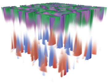


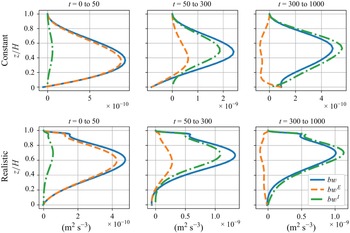


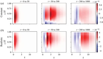


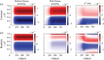


 Open access