





1. Introduction
Acoustic liners are extensively used in aircraft engines as a passive noise control devices to reduce noise emissions (Motsinger & Kraft Reference Motsinger and Kraft1991; Winkler et al. Reference Winkler, Mendoza, Reimann, Homma and Alonso2021); they are usually installed in the intake of engines and in the core jet section. The noise source in aircraft engines consists of two main components: a tonal component at the blade-passing frequency (BPF) and a broadband component generated by turbulence impingement, which arises from the close proximity of the fan to the stator stage (Mallat Reference Mallat1989; Hughes Reference Hughes2011; Casalino, Hazir & Mann Reference Casalino, Hazir and Mann2017). Recent development of ultra-high-bypass-ratio engines, characterised by a larger fan diameter compared with traditional high-bypass-ratio engines, has significantly increased the contribution of fan noise to the overall engine noise.
The simplest acoustic liner is the single-degree-of-freedom (SDOF) one, which comprises a cavity backing and a perforated face-sheet (Motsinger & Kraft Reference Motsinger and Kraft1991). In the absence of grazing turbulent flow and high-intensity acoustic waves, a conventional SDOF liner behaves like a Helmholtz resonator. The presence of acoustic waves at a frequency close to that of resonance excites an acoustic-induced flow within the orifice that leads to acoustic dissipation (Tam & Kurbatskii Reference Tam and Kurbatskii2000). The resonant frequency of the liner is typically tuned to coincide with the fan’s BPF or its harmonics, making SDOF liners particularly suitable for fan noise attenuation. The response of acoustic liners is typically characterised through the impedance, which depends on geometric parameters, sound pressure level (SPL) and flow conditions (Quintino et al. Reference Quintino, Bonomo, Cordioli, Jones, Howerton, Nark and Avallone2025).
The physics of acoustic liners and their dissipation mechanism is well established when they are exposed solely to acoustic waves (Melling Reference Melling1973; Tam & Kurbatskii Reference Tam and Kurbatskii2000); however, a gap persists in the understanding and modelling of noise dissipation when the liners operate under real working conditions, i.e. in the presence of both acoustic wave and grazing turbulent flow at high Mach numbers and SPL. In the absence of grazing flow, impedance can be directly linked with the absorption coefficient and thus energy dissipation; however, this relation does not hold when the liner works in the presence of grazing flow and at high SPL (Tam et al. Reference Tam, Ju, Jones, Watson and Parrott2009).
In the absence of grazing flow, energy dissipation in an SDOF liner occurs through viscous losses and via vortex shedding mechanisms. For moderate SPLs, typically below $140\,\mathrm{dB}$
, viscous dissipation dominates; it occurs along the internal surfaces of the orifices where laminar boundary layers develop (Tam & Kurbatskii Reference Tam and Kurbatskii2000). As the SPL increases and the operating regime transitions into a fully nonlinear one, the acoustic-induced flow topology is characterised by the emergence of turbulent jets and the shedding of vortices at the orifice entrances (Tam & Kurbatskii Reference Tam and Kurbatskii2000; Zhang & Bodony Reference Zhang and Bodony2012). Here, acoustic energy is transformed into turbulent kinetic energy associated with the rotational motion of vortices, which is ultimately dissipated as heat through viscous processes (Tam & Kurbatskii Reference Tam and Kurbatskii2000). According to Tam & Kurbatskii (Reference Tam and Kurbatskii2000), vortex shedding is amplified near the liner’s resonant frequency, but remains largely unaffected by the angle of incidence of the acoustic waves. Recent experimental investigations without grazing flow, such as that by Tang, Wang & Liu (Reference Tang, Wang and Liu2024), have revealed the presence of multi-scale vortex structures driven by an acoustic excitation at high SPL.
$140\,\mathrm{dB}$
, viscous dissipation dominates; it occurs along the internal surfaces of the orifices where laminar boundary layers develop (Tam & Kurbatskii Reference Tam and Kurbatskii2000). As the SPL increases and the operating regime transitions into a fully nonlinear one, the acoustic-induced flow topology is characterised by the emergence of turbulent jets and the shedding of vortices at the orifice entrances (Tam & Kurbatskii Reference Tam and Kurbatskii2000; Zhang & Bodony Reference Zhang and Bodony2012). Here, acoustic energy is transformed into turbulent kinetic energy associated with the rotational motion of vortices, which is ultimately dissipated as heat through viscous processes (Tam & Kurbatskii Reference Tam and Kurbatskii2000). According to Tam & Kurbatskii (Reference Tam and Kurbatskii2000), vortex shedding is amplified near the liner’s resonant frequency, but remains largely unaffected by the angle of incidence of the acoustic waves. Recent experimental investigations without grazing flow, such as that by Tang, Wang & Liu (Reference Tang, Wang and Liu2024), have revealed the presence of multi-scale vortex structures driven by an acoustic excitation at high SPL.
A detailed understanding of the acoustic response of liners subjected to high-speed turbulent grazing flow and acoustic waves remains incomplete. Under these conditions, liners operate always in the nonlinear regime despite the SPL at which they are exposed, and the coupling between flow and acoustics becomes increasingly complex. In particular, the spatial and temporal evolution of the velocity field inside the orifices deviates substantially from the no-flow case (Zhang & Bodony Reference Zhang and Bodony2016b ). The interaction between the acoustic-induced flow field and the grazing flow was visualised for the first time by Baumeister & Rice (Reference Baumeister and Rice1975). They identified the presence of a vortex at the upstream side of the orifice neck, leading to a reduction in the effective inflow area. Subsequent computational studies have explored the flow physics inside the orifice in greater detail. Initial investigations focused on simplified configurations without grazing flow (Tam & Kurbatskii Reference Tam and Kurbatskii2000) and later were extended to include grazing flow conditions.
Shahzad, Hickel & Modesti (Reference Shahzad, Hickel and Modesti2023) performed direct numerical simulations of a turbulent grazing flow over a lined wall in the absence of acoustic forcing, revealing substantial modifications of the near-wall flow topology compared with a smooth surface. This was linked with an increase in drag. Fully three-dimensional (3-D) numerical simulations examining the interaction between acoustic waves and grazing flow over an acoustic liner were performed by Zhang & Bodony (Reference Zhang and Bodony2016b ). The simulations elucidated the intricate coupling between the flow field and the liner’s acoustic response, and how this coupling depends on the state of the incoming boundary layer, laminar or turbulent. Their results showed that the influence of boundary-layer parameters is more pronounced at low SPL. In addition, they showed the ejection of vorticity both outside the liner and into the liner cavity through the orifice, an effect that becomes increasingly more pronounced at high SPL, where the influence of the grazing flow weakens. Using micro-particle image velocimetry, Léon et al. (Reference Léon, Méry, Piot and Conte2019) investigated how a turbulent grazing flow interacts with a conventional acoustic liner under acoustic excitation. At low SPL, the grazing flow remained essentially unaffected, whereas at higher SPL, the acoustic forcing produced mean-flow distortions above the orifice and synthetic-jet-like motions penetrating deeply into the grazing flow. The local state of the turbulent grazing flow, in turn, strongly influences the spatial decay of the SPL along a lined duct. Recent studies by Paduano et al. (Reference Paduano, Scarano, Cordioli, Casalino and Avallone2026b ) confirmed that the SPL decays less in the presence of flow over an acoustic liner, suggesting that the underlying noise dissipation mechanisms are locally modified by the near-wall flow features.
Despite extensive research efforts, a comprehensive description of the flow dynamics within the liner’s orifices and a reliable quantification of acoustic dissipation mechanisms under grazing flow are still lacking. This challenge arises mainly from the difficulty of resolving fine-scale flow features, such as the vorticity field and wall shear stresses on the perforated plate. High-fidelity numerical simulations, complemented by controlled experiments, therefore offer a powerful approach to investigate these phenomena and deepen our understanding of the noise dissipation mechanisms.
In this study, we aim to quantify the contributions of both vortex shedding and viscous dissipation to the overall acoustic energy dissipation. We compare configurations with and without grazing flow and explore the effect of varying SPL, source frequency and acoustic propagation direction, covering both the linear and nonlinear regimes. The main research questions guiding this work are the following.
-
(i) How does the presence of grazing flow alter the dissipation of acoustic energy in an acoustic liner?
-
(ii) How does the change in flow topology inside the orifice influence the dissipation mechanism?
-
(iii) How do the relative contributions of viscous effects at the orifice walls and vortex shedding vary in the presence of grazing flow, and what is the impact of changing the SPL?
The dissipation by viscous effects at the orifice walls is evaluated following the approach proposed by Tam & Kurbatskii (Reference Tam and Kurbatskii2000), while the dissipation by vortex shedding is evaluated applying Howe’s energy corollary (Howe Reference Howe1980). Howe’s energy corollary has been previously applied to highlight the mechanisms of generation and absorption of sound in air-jet instruments relying on both numerical (Tabata et al. Reference Tabata, Matsuda, Koiwaya, Iwagami, Midorikawa, Kobayashi and Takahashi2021) and experimental (Yoshikawa, Tashiro & Sakamoto Reference Yoshikawa, Tashiro and Sakamoto2012) data.
The analysis are applied to high-fidelity data obtained with lattice-Boltzmann very-large-eddy simulations (LB/VLES) of a fully resolved liner configuration, consisting of a single cavity and a perforated plate with multiple orifices. This configuration reduces computational cost while focusing on the dissipation mechanisms of interest. By analysing a single orifice within one cavity, we can isolate the direct effect of the grazing flow itself from the additional complexities introduced by the development of the flow over a full liner (Shahzad, Hickel & Modesti Reference Shahzad, Hickel and Modesti2025; Paduano et al. Reference Paduano, Scarano, Cordioli, Casalino and Avallone2026b ). The liner geometry replicates that used in previous experimental campaigns conducted in the Grazing Flow Impedance Tube (GFIT) facility at NASA Langley Research Center (Jones, Watson & Nark Reference Jones, Watson and Nark2010), as well as in the numerical studies by Zhang & Bodony (Reference Zhang and Bodony2016b ).
The paper is organised as follows. Section 2 describes the data reduction methodology, the technique to evaluate the acoustic-induced velocity, and the methods used to quantify dissipation due to vortex shedding and viscous effects. Section 3 outlines the numerical set-up, solver details, geometry and the simulation test matrix. Section 4 focuses on the flow field inside the orifices, examining both the acoustic-induced velocity distribution inside the orifice and the shear layer development at the orifice mouth. Section 5 presents the parametric analysis of the dissipation mechanisms when varying the SPL value, while § 6 investigates the effect of changing source frequency, propagation direction and the interference between two consecutive orifices. Section 7 concludes the paper.
2. Data reduction methodology
2.1. Nomenclature for velocity components
Considering the time-resolved nature of the analysis, the instantaneous velocity field is denoted by $\boldsymbol{u}'$
and is decomposed as
$\boldsymbol{u}'$
and is decomposed as
 \begin{align} \boldsymbol{u}' = \boldsymbol{U} + \boldsymbol{u}, \end{align}
where $\boldsymbol{U}$
is the mean velocity and
$\boldsymbol{U}$
is the mean velocity and $\boldsymbol{u}$
represents the fluctuating component. The instantaneous velocity components
$\boldsymbol{u}$
represents the fluctuating component. The instantaneous velocity components $(u',v',w')$
are in the three spatial directions
$(u',v',w')$
are in the three spatial directions $(x,y,z)$
. Accordingly,
$(x,y,z)$
. Accordingly, $U, V, W$
are the time-averaged velocity components and
$U, V, W$
are the time-averaged velocity components and $u, v, w$
the fluctuating components following the Reynolds decomposition.
$u, v, w$
the fluctuating components following the Reynolds decomposition.
In the presence of acoustic forcing, the fluctuating velocity $\boldsymbol{u}$
includes two contributions: the turbulent (aerodynamic) fluctuations and the acoustic-induced velocity
$\boldsymbol{u}$
includes two contributions: the turbulent (aerodynamic) fluctuations and the acoustic-induced velocity $\boldsymbol{u}_{{ac}}$
, which arises from the periodic forcing (Scarano et al. Reference Scarano, Lyu, Paduano and Avallone2026).
$\boldsymbol{u}_{{ac}}$
, which arises from the periodic forcing (Scarano et al. Reference Scarano, Lyu, Paduano and Avallone2026).
2.2. Acoustic dissipation by viscous effects
The rate of mechanical energy dissipation due to viscosity is evaluated from the instantaneous velocity field following the approach of Tam & Kurbatskii (Reference Tam and Kurbatskii2000). In a three-dimensional framework, the local volumetric viscous dissipation density is defined as
 \begin{align} \varPhi (\boldsymbol{x},t) = \sigma _{\textit{ij}}(\boldsymbol{x},t) \frac {\partial u^{\prime}_i}{\partial x_{\!j}}, \end{align}
where the viscous stress tensor is
 \begin{align} \sigma _{\textit{ij}}(\boldsymbol{x},t) = \mu \left ( \frac {\partial u^{\prime}_i}{\partial x_{\!j}} + \frac {\partial u^{\prime}_{\!j}}{\partial x_i} \right ), \end{align}
where $\mu$
is the dynamic viscosity,
$\mu$
is the dynamic viscosity, $i,j=1,2,3$
are the indices of the three spatial directions and
$i,j=1,2,3$
are the indices of the three spatial directions and $u^{\prime}_i$
is the instantaneous velocity component, and
$u^{\prime}_i$
is the instantaneous velocity component, and $\boldsymbol{x}= (x,y,z)$
denotes the spatial position vector. The quantity
$\boldsymbol{x}= (x,y,z)$
denotes the spatial position vector. The quantity $\varPhi (\boldsymbol{x},t)$
has units of power density (
$\varPhi (\boldsymbol{x},t)$
has units of power density ( $\mathrm{W\,m^{-3}}$
) and represents the irreversible conversion of mechanical energy into internal energy due to viscous effects.
$\mathrm{W\,m^{-3}}$
) and represents the irreversible conversion of mechanical energy into internal energy due to viscous effects.
The imposed acoustic forcing induces an oscillatory motion within the orifice, which in turn generates time-dependent velocity gradients within the near-wall region of the orifice; these oscillations are responsible for the additional viscous dissipation associated with the acoustic field. To isolate the acoustically induced viscous losses and exclude the viscous dissipation associated solely to the aerodynamic development of the turbulent grazing flow, the integration volume is restricted to a near-wall region adjacent to the orifice side walls, extending up to approximately 30 wall units (corresponding to $\Delta x/d \lt 0.09$
). This choice follows the formulation adopted for resonant liners, where the portion of acoustic energy dissipated into heat by viscous effects is primarily attributed to near-wall processes within the orifice neck (Tam & Kurbatskii Reference Tam and Kurbatskii2000). The adopted control volume therefore captures both the near-wall gradients provided by the wall model and the viscous stresses within the boundary layer inside the orifice, including turbulent contributions injected from the grazing flow.
$\Delta x/d \lt 0.09$
). This choice follows the formulation adopted for resonant liners, where the portion of acoustic energy dissipated into heat by viscous effects is primarily attributed to near-wall processes within the orifice neck (Tam & Kurbatskii Reference Tam and Kurbatskii2000). The adopted control volume therefore captures both the near-wall gradients provided by the wall model and the viscous stresses within the boundary layer inside the orifice, including turbulent contributions injected from the grazing flow.
The three-dimensional integration domain is shown in Appendix D. The viscous dissipation rate in a control volume $V$
enclosing the orifice and the region in proximity of the orifice internal walls is therefore
$V$
enclosing the orifice and the region in proximity of the orifice internal walls is therefore
 \begin{align} D(t) = \iiint _V \varPhi (\boldsymbol{x},t) \,\mathrm{d}V. \end{align}
Dissipation occurring in the bulk flow through the orifice, associated with the subsequent decay of vortical structures through the turbulent cascade, is not directly included in the viscous term. Its energetic contribution is instead represented through the vortex-shedding analysis based on Howe’s corollary, which quantifies the transfer of acoustic energy into vortical motion.
The phase-dependent viscous dissipation rate is obtained by phase-averaging $D(t)$
over one acoustic period and is denoted as
$D(t)$
over one acoustic period and is denoted as $D(\phi )$
. The net viscous energy dissipated per unit time over one oscillation period
$D(\phi )$
. The net viscous energy dissipated per unit time over one oscillation period $T$
is
$T$
is
 \begin{align} E_{\textit{viscous}} = \frac {1}{T} \int _0^T D(\phi )\,\mathrm{d}\phi . \end{align}
All viscous dissipation related quantities are normalised in wall units using the friction velocity $u_\tau =\sqrt {\tau _w/\rho }$
, where
$u_\tau =\sqrt {\tau _w/\rho }$
, where $\tau _w$
is the wall shear stress and
$\tau _w$
is the wall shear stress and $\rho$
is the fluid density, and the viscous scale
$\rho$
is the fluid density, and the viscous scale $\delta _\nu = \nu /u_\tau$
, where
$\delta _\nu = \nu /u_\tau$
, where $ \nu$
the kinematic viscosity. These quantities are computed for the smooth baseline case without acoustic. The local volumetric dissipation density is normalised as
$ \nu$
the kinematic viscosity. These quantities are computed for the smooth baseline case without acoustic. The local volumetric dissipation density is normalised as
 \begin{align} \varPhi ^{+}(\phi ) = \frac {\varPhi }{\rho u_\tau ^4/\nu }, \end{align}
while the volume integrated dissipation rate is normalised as
 \begin{align} D^{+}(\phi ) = \frac {D}{\rho \nu ^2 u_\tau }. \end{align}
2.3. Acoustic energy conversion into vortex shedding
The conversion of acoustic energy into vortical motion is quantified using Howe’s energy corollary (Howe Reference Howe1975, Reference Howe1980, Reference Howe1984). The local volumetric power density transferred from the acoustic field to the vortical field is given by
 \begin{align} \varPi _g(\boldsymbol{x},t) = \rho \left ( \boldsymbol{\omega } \times \boldsymbol{u}' \right ) \boldsymbol{\cdot }\boldsymbol{u}_{{ac}}, \end{align}
where $\boldsymbol{\omega }$
is the vorticity,
$\boldsymbol{\omega }$
is the vorticity, $\boldsymbol{u}_{{ac}}$
is the acoustic-induced velocity fluctuation field and
$\boldsymbol{u}_{{ac}}$
is the acoustic-induced velocity fluctuation field and $\boldsymbol{u'}$
is the instantaneous velocity vector.
$\boldsymbol{u'}$
is the instantaneous velocity vector.
The total acoustic energy conversion rate within the control volume $V$
is defined as
$V$
is defined as
 \begin{align} \varPi (t) = \iiint _V \varPi _g(\boldsymbol{x},t) \,\mathrm{d}V. \end{align}
The control volume is chosen such to include the shear layer forming at the orifice mouth, the orifice and cavity regions, and the portion of the grazing boundary layer interacting directly with the orifice. This ensures that the acoustic–vortical interaction associated with the dominant structures is fully captured.
The phase-dependent quantity $\varPi ^+(\phi )$
is obtained by phase-averaging over one acoustic cycle. The net energy transferred per unit time over one period
$\varPi ^+(\phi )$
is obtained by phase-averaging over one acoustic cycle. The net energy transferred per unit time over one period $T$
is
$T$
is
 \begin{align} E_{\textit{shedding}} = \frac {1}{T} \int _0^T \varPi (\phi )\,\mathrm{d}\phi . \end{align}
The local power density converted into the vortical field is normalised in wall units as
 \begin{align} \varPi _g^{+} = \frac {\varPi _g}{\rho u_\tau ^4/\nu }, \end{align}
while the integrated conversion rate is normalised as
 \begin{align} \varPi ^{+} = \frac {\varPi }{\rho \nu ^2 u_\tau }. \end{align}
A positive value of $\varPi ^+_g$
or
$\varPi ^+_g$
or $\varPi ^+$
indicates absorption of acoustic energy by the vortical field, whereas a negative value indicates acoustic energy generation.
$\varPi ^+$
indicates absorption of acoustic energy by the vortical field, whereas a negative value indicates acoustic energy generation.
2.4. Acoustic-induced velocity estimation
To evaluate Howe’s energy corollary, it is necessary to isolate the velocity component induced by the imposed acoustic forcing from the fluctuations generated by the turbulent grazing flow. The acoustic-induced velocity field is extracted using spectral proper orthogonal decomposition (SPOD) (Schmidt & Colonius Reference Schmidt and Colonius2020), following the methodology detailed by Scarano et al. (Reference Scarano, Lyu, Paduano and Avallone2026).
SPOD is applied using as input the fluctuating component of the velocity field. SPOD provides a set of frequency-dependent orthogonal modes ranked by their spectral energy content. The acoustic-induced velocity is reconstructed by selecting the leading SPOD mode associated with the known forcing frequency and performing a narrow bandpass reconstruction centred at that frequency. This procedure isolates the velocity component that is coherent and phase-locked with the imposed acoustic excitation.
As demonstrated by Scarano et al. (Reference Scarano, Lyu, Paduano and Avallone2026), for datasets characterised by a single dominant acoustic forcing and in the absence of additional tonal sources (e.g. self-sustained tones), SPOD yields results equivalent to those obtained with the recently developed canonical correlation decomposition (CCD) by Nie, Yao & Lyu (Reference Nie, Yao and Lyu2026), which identifies the acoustic velocity as the component that best correlates with the forcing signal. Under these conditions, both approaches provide a consistent estimate of the acoustically driven velocity field.
In many liner studies (e.g. Zhang & Bodony Reference Zhang and Bodony2012; Léon et al. Reference Léon, Méry, Piot and Conte2019), the acoustic velocity is obtained by phase locking the data using a triple-decomposition approach. However, in the presence of grazing turbulent flow and high SPLs, the SPOD-based approach has been shown to provide a more robust separation between coherent acoustic motion and broadband turbulent fluctuations (Scarano et al. Reference Scarano, Lyu, Paduano and Avallone2026), without assuming linearity or irrotationality.
It is important to clarify that the term ‘acoustic-induced velocity’ refers here to the velocity component coherent with the forcing frequency, rather than to a strictly irrotational field. A Helmholtz decomposition or a reconstruction based on the acoustic Euler equations (Schoder, Roppert & Kaltenbacher Reference Schoder, Roppert and Kaltenbacher2020; Unnikrishnan & Gaitonde Reference Unnikrishnan and Gaitonde2020) would require full three-dimensional information on the velocity divergence and appropriate boundary conditions. Such requirements are not satisfied for the two-dimensional (2-D) extracted planes considered in the parametric analysis and the underlying assumptions are not strictly valid in strongly nonlinear flow–acoustic interaction regimes. The SPOD-based approach therefore provides a physically consistent and practically robust method to extract the velocity component relevant to the acoustic energy-transfer analysis carried out in this study.
3. Numerical set-up and database description
3.1. Numerical solver
The simulations are performed using a lattice Boltzmann method (LBM) solver combined with a very large eddy simulation (VLES) approach. This methodology is selected as a compromise between linearised frequency-domain methods and fully resolved simulations. Classical liner simulations, based on linearised governing equations, are very efficient for predicting the frequency-dependent liner response in terms of impedance under small-amplitude perturbations. However, by construction, they neglect SPL-induced nonlinearities and therefore are not appropriate when the liner is exposed to high SPL. In addition, they commonly assume a prescribed base flow (often a steady sheared profile (Myers Reference Myers1980; Gabard Reference Gabard2016)) that is only weakly influenced by the liner surface and does not fully represent the mutual coupling between the grazing boundary layer and the liner treatment (Tam et al. Reference Tam, Ju, Jones, Watson and Parrott2009).
At the opposite end, highly resolved approaches such as direct numerical simulation (DNS) resolve the full nonlinear flow–acoustic interaction, but their computational cost is prohibitive for the Reynolds numbers and parametric space of practical interest.
From a practical standpoint, the LBM framework offers low numerical dissipation for acoustic wave propagation, efficient parallelisation and automatic Cartesian meshing. These features, combined with the VLES turbulence treatment, make it possible to perform parametric studies over a wide range of SPLs and frequencies at a tractable computational cost, while retaining the essential physics of the flow–acoustic interaction.
The commercial software 3DS Simulia PowerFLOW 6–2019R4 is used to compute the flow and acoustic field. PowerFLOW simulation technology is based on an LB method with collision relaxation time and distribution function dynamically calibrated to the time scales of slow turbulent structures modelled through a turbulence transport model. The solver has already been validated for canonical honeycomb liner configurations, both in the absence of flow (Mann et al. Reference Mann, Perot, Kim and Casalino2013; Hazir & Casalino Reference Hazir and Casalino2017) and with grazing flow (Manjunath et al. Reference Manjunath, Avallone, Casalino, Ragni and Snellen2018; Avallone et al. Reference Avallone, Manjunath, Ragni and Casalino2019). The same solver has also been used to simulate the effect of an SDOF liner installed on the nacelle of the NASA Source Diagnostic Test engine configuration (Casalino et al. Reference Casalino, Hazir and Mann2017), and the predicted sound attenuation has recently been confirmed by another simulation carried out by using a different high-fidelity flow solver (Shur et al. Reference Shur, Strelets, Travin, Suzuki and Spalart2021).
The LB scheme is based on an expansion of the distribution function $f\! ( {\boldsymbol{x}},{\boldsymbol \xi },t )$
, say the probability density of finding particles at location
$f\! ( {\boldsymbol{x}},{\boldsymbol \xi },t )$
, say the probability density of finding particles at location $\boldsymbol{x}$
, advected at velocity
$\boldsymbol{x}$
, advected at velocity $\boldsymbol \xi$
at time
$\boldsymbol \xi$
at time $t$
, solution of the Boltzmann equation, in a series of Hermite polynomials (Shan, Yuan & Chen Reference Shan, Yuan and Chen2006). These constitute an orthogonal basis, which is particularly suited to describe a flow in the kinetic space. Indeed, the first four coefficients, from zeroth to thrid order, of the expansion of the Maxwellian distribution function
$t$
, solution of the Boltzmann equation, in a series of Hermite polynomials (Shan, Yuan & Chen Reference Shan, Yuan and Chen2006). These constitute an orthogonal basis, which is particularly suited to describe a flow in the kinetic space. Indeed, the first four coefficients, from zeroth to thrid order, of the expansion of the Maxwellian distribution function $f^{(0)}$
at equilibrium are algebraically related to the moments of macroscopic flow, say mass, momentum, energy/momentum fluxes and heat fluxes. An interesting property of a Hermite expansion is that the series can be truncated at a given order without altering the low-order coefficients; therefore, an expansion of
$f^{(0)}$
at equilibrium are algebraically related to the moments of macroscopic flow, say mass, momentum, energy/momentum fluxes and heat fluxes. An interesting property of a Hermite expansion is that the series can be truncated at a given order without altering the low-order coefficients; therefore, an expansion of $f$
truncated at the order
$f$
truncated at the order $N\!\gt \!3$
provides a unique representation of the macroscopic hydrodynamic status of a fluid.
$N\!\gt \!3$
provides a unique representation of the macroscopic hydrodynamic status of a fluid.
A key component of the PowerFLOW LB scheme is the usage of a regularised collision operator $\varOmega _i$
in the non-dimensional lattice Boltzmann equation
$\varOmega _i$
in the non-dimensional lattice Boltzmann equation
 \begin{align} f_i\!\left ( {\boldsymbol{x}}+{\boldsymbol \xi }_i,t+1 \right )\!=\!f_i\!\left ( {\boldsymbol{x}},t \right )\!+\!\varOmega _i, \end{align}
projected along the discrete particle velocity ${\boldsymbol \xi }_i$
. Following Zhang, Shan & Chen (Reference Zhang, Shan and Chen2006), the LB equation can be equivalently written as
${\boldsymbol \xi }_i$
. Following Zhang, Shan & Chen (Reference Zhang, Shan and Chen2006), the LB equation can be equivalently written as
 \begin{align} f_i\!\left ( {\boldsymbol{x}}+{\boldsymbol \xi }_i,t+1 \right )\!=\!f^{(0)}_i\!\left ( {\boldsymbol{x}},t \right )\!+\!f^{(1)}_i\!\left ( {\boldsymbol{x}},t \right )\!+\!\varOmega _i, \end{align}
where $f^{(1)}_i$
is the perturbation. In conditions that are not very far from equilibrium, the collision operator is linearly related to the perturbation through coefficients that are negatively/inversely proportional to relaxation time
$f^{(1)}_i$
is the perturbation. In conditions that are not very far from equilibrium, the collision operator is linearly related to the perturbation through coefficients that are negatively/inversely proportional to relaxation time $\tau _{\textit{ij}}$
of the collision process along the discrete velocity direction
$\tau _{\textit{ij}}$
of the collision process along the discrete velocity direction $i$
due to chaotic motion along the direction
$i$
due to chaotic motion along the direction $j$
, say
$j$
, say
 \begin{align} f_i\!\left ( {\boldsymbol{x}}+{\boldsymbol \xi }_i,t+1 \right )\!=\!f^{(0)}_i\!\left ( {\boldsymbol{x}},t \right )\!+\!\sum _{\!j}\left ( \delta _{\textit{ij}}-1/\tau _{\textit{ij}} \right )f^{(1)}_i\!\left ( {\boldsymbol{x}},t \right ). \end{align}
If the perturbation is expanded in Hermite series, this starts by the second-order term and can be truncated at the third-order term to recover the macroscopic fluid status. The resulting regularised collision operator will therefore include only terms proportional to the second-order Hermite polynomials, accounting for energy and momentum fluxes, and third-order term polynomials, accounting for heat fluxes. Finally, following Chen, Gopalakrishnan & Zhang (Reference Chen, Gopalakrishnan and Zhang2014), applying Galilean invariance to the collision operator results in a two-term regularised form, in which the two terms account for energy/momentum fluxes and heat fluxes, respectively, with corresponding relaxation times related to the macroscopic fluid viscosity and thermal conductivity.
Another important component of the present flow simulation methodology is related to turbulence modelling, which is key to tackle high-Reynolds-number flows. The way turbulence is accounted for in PowerFLOW is by modifying the relaxation time in the collision operator by considering the time scales related to the turbulent motion and to the strain rate and rotation of the resolved flow field. Moreover, the amount of turbulent kinetic energy is used to define the equilibrium state of the gas. As discussed by Chen et al. (Reference Chen, Orszag, Staroselsky and Succi2004), the expansion of kinetic theory from particles to eddies leads to the fundamental observation that the Reynolds stresses, which are a consequence of chaotic turbulent motion, have a nonlinear structure and are better suited to represent turbulence in states far from equilibrium, such as in the presence of distortion, shear, separation, curvature or rotation. At first order, the kinetic expansion recovers the classical eddy-viscosity form
 \begin{align} \sigma _{\textit{ij}}^{(1)} = 2\nu _t S_{\textit{ij}}, \end{align}
where
 \begin{align} S_{\textit{ij}} = \frac {1}{2} \left ( \frac {\partial u^{\prime}_i}{\partial x_{\!j}} + \frac {\partial u^{\prime}_{\!j}}{\partial x_i} \right ) \end{align}
is the resolved strain-rate tensor, and the turbulent viscosity can be expressed as
 \begin{align} \nu _t = \frac {2}{3}k\tau _t. \end{align}
If the turbulent relaxation time is estimated from a two-equation model, such as the RNG $k$
–
$k$
– $\epsilon$
model, one may write
$\epsilon$
model, one may write
 \begin{align} \tau _t = \frac {3}{2}C_\mu \frac {k}{\epsilon }, \qquad \nu _t = C_\mu \frac {k^2}{\epsilon }. \end{align}
However, although the relaxation time is computed using the two-equation $k$
–
$k$
– $\epsilon$
re-normalisation group, RNG, model in PowerFLOW (Yakhot et al. Reference Yakhot, Orszag, Thangam, Gatski and Speziale1992; Teixeira Reference Teixeira1998), this model is not employed to compute an equivalent eddy viscosity in the same sense as in traditional Reynolds-averaged Navier–Stokes, RANS, formulations. In standard RANS models,
$\epsilon$
re-normalisation group, RNG, model in PowerFLOW (Yakhot et al. Reference Yakhot, Orszag, Thangam, Gatski and Speziale1992; Teixeira Reference Teixeira1998), this model is not employed to compute an equivalent eddy viscosity in the same sense as in traditional Reynolds-averaged Navier–Stokes, RANS, formulations. In standard RANS models, $\nu _t$
is used to explicitly close the Reynolds stresses in the averaged momentum equations. In the LB/VLES formulation, instead, the turbulence model is used to dynamically recalibrate the Boltzmann relaxation process to the characteristic time scales of the unresolved turbulent motion.
$\nu _t$
is used to explicitly close the Reynolds stresses in the averaged momentum equations. In the LB/VLES formulation, instead, the turbulence model is used to dynamically recalibrate the Boltzmann relaxation process to the characteristic time scales of the unresolved turbulent motion.
The key advantage of this kinetic interpretation is that the Reynolds stresses are not restricted to a purely linear eddy-viscosity form. As shown by Chen et al. (Reference Chen, Orszag, Staroselsky and Succi2004), a second-order expansion of the kinetic model gives
 \begin{align} \sigma _{\textit{ij}} &\approx -\frac {2}{3}k\delta _{\textit{ij}} + 2\nu _t S_{\textit{ij}} - 2\nu _t \frac {\rm D}{{\rm D}t} \left ( \tau _t S_{\textit{ij}} \right ) - 6\frac {\nu _t^2}{k} \left ( S_{\textit{ik}}S_{\textit{kj}} - \frac {1}{3}\delta _{\textit{ij}}S_{\textit{kl}}S_{\textit{kl}} \right )\notag\\&\quad + 3\frac {\nu _t^2}{k} \left ( S_{\textit{ik}}\varOmega _{kj} + S_{\textit{jk}}\varOmega _{\textit{ki}} \right ), \end{align}
where
 \begin{align} \varOmega _{\textit{ij}} = \frac {1}{2} \left ( \frac {\partial u^{\prime}_i}{\partial x_{\!j}} - \frac {\partial u^{\prime}_{\!j}}{\partial x_i} \right ) \end{align}
is the resolved rotation-rate tensor and
 \begin{align} \frac {\rm D}{{\rm D}t} = \frac {\partial }{\partial t} + \boldsymbol{u'}\boldsymbol{\cdot }\boldsymbol{\nabla }\end{align}
is the material derivative following the resolved flow. Equation (3.8) shows that the turbulent stress contains not only the classical linear contribution $2\nu _t S_{\textit{ij}}$
, but also memory, strain–strain and strain–rotation effects. The memory term accounts for the finite time required by the turbulent eddies to relax towards equilibrium, while the nonlinear terms describe the response of the unresolved turbulent motion to strong deformation and rotation of the resolved flow.
$2\nu _t S_{\textit{ij}}$
, but also memory, strain–strain and strain–rotation effects. The memory term accounts for the finite time required by the turbulent eddies to relax towards equilibrium, while the nonlinear terms describe the response of the unresolved turbulent motion to strong deformation and rotation of the resolved flow.
Hence, no Reynolds stresses are explicitly added to the governing equations. Rather, their effect emerges implicitly through the non-equilibrium momentum exchange produced by the modified collision operator. In the present study, the LBM equations are discretised on a Cartesian grid whose volume elements are voxels. The adopted numerical scheme is the D3Q19 lattice, where ‘D3’ denotes three spatial dimensions and ‘Q19’ the number of discrete velocity directions (Qian, D’Humières & Lallemand Reference Qian, D’Humières and Lallemand1992). Accordingly, the total number of degrees of freedom (DOFs) is directly related to the number of voxels in the computational domain (and to the 19 distribution functions stored per voxel in the D3Q19 formulation).
3.2. Wall model
The simulations employ a pressure-gradient-extended turbulent wall model (PGE-WM), following the formulation of Teixeira (Reference Teixeira1998). This approach modifies the classical logarithmic law-of-the-wall to account for the influence of streamwise pressure gradients on the near-wall velocity distribution.
In the generalised formulation, the inner-scaled velocity is expressed as
 \begin{align} U^+ = \frac {1}{k} \ln \!\left (\frac {y^+}{A}\right ) + B, \end{align}
where $k$
and
$k$
and $B$
are the von Kármán constant and additive constant, respectively, and
$B$
are the von Kármán constant and additive constant, respectively, and $y^+=u_\tau y/\nu$
is the viscous wall-normal coordinate and
$y^+=u_\tau y/\nu$
is the viscous wall-normal coordinate and $u_ \tau$
is the friction velocity. The factor
$u_ \tau$
is the friction velocity. The factor $A$
introduces a correction to the standard logarithmic profile to capture the modification of the near-wall structure induced by pressure gradients.
$A$
introduces a correction to the standard logarithmic profile to capture the modification of the near-wall structure induced by pressure gradients.
Physically, the presence of a streamwise pressure gradient alters the development of the boundary layer by modifying the local velocity gradient and effectively stretching or compressing the inner-scaled profile. This effect is incorporated through the scaling parameter $A$
, defined as
$A$
, defined as
 \begin{align} A &= 1 + \frac {\beta \,\left |\frac {\mathrm{d}p}{\mathrm{d}s}\right |}{\tau _w} \quad \text{if } \boldsymbol{\hat {u}'}\boldsymbol{\cdot }\frac {\mathrm{d}p}{\mathrm{d}s} \gt 0, \end{align}
 \begin{align} A &= 1 \quad \text{otherwise}, \end{align}
where $\tau _w$
denotes the wall shear stress,
$\tau _w$
denotes the wall shear stress, $\mathrm{d}p/\mathrm{d}s$
is the streamwise pressure gradient,
$\mathrm{d}p/\mathrm{d}s$
is the streamwise pressure gradient, $\boldsymbol{\hat {u}'}$
is the unit vector of the local velocity and
$\boldsymbol{\hat {u}'}$
is the unit vector of the local velocity and $\beta$
is a length scale representative of the unresolved near-wall region. The condition
$\beta$
is a length scale representative of the unresolved near-wall region. The condition $\boldsymbol{\hat {u}'}\boldsymbol{\cdot }( {\mathrm{d}p}/{\mathrm{d}s}) \gt 0$
identifies an adverse pressure gradient, for which the pressure increases in the direction of the local near-wall flow. The use of the unit vector ensures that this condition depends only on the direction of the flow and not on its magnitude. The magnitude of the correction is instead governed by the non-dimensional ratio
$\boldsymbol{\hat {u}'}\boldsymbol{\cdot }( {\mathrm{d}p}/{\mathrm{d}s}) \gt 0$
identifies an adverse pressure gradient, for which the pressure increases in the direction of the local near-wall flow. The use of the unit vector ensures that this condition depends only on the direction of the flow and not on its magnitude. The magnitude of the correction is instead governed by the non-dimensional ratio $\beta | {\mathrm{d}p}/{\mathrm{d}s}|/\tau _w$
, which compares the pressure-gradient contribution across the unresolved near-wall region with the local wall shear stress.
$\beta | {\mathrm{d}p}/{\mathrm{d}s}|/\tau _w$
, which compares the pressure-gradient contribution across the unresolved near-wall region with the local wall shear stress.
This formulation enables the wall model to dynamically adjust to adverse or favourable pressure-gradient conditions while preserving the structure of the logarithmic law in the absence of pressure gradients. Confidence in the numerical framework is provided by the work by Paduano et al. (Reference Paduano, Scarano, Cordioli, Casalino and Avallone2026b ), where the same LB–VLES approach is applied to a more complex configuration involving a full acoustic liner. That study demonstrates that this numerical framework accurately reproduces experimental measurements of SPL decay and acoustic impedance (Quintino et al. Reference Quintino, Bonomo, Cordioli, Jones, Howerton, Nark and Avallone2025), indicating that the overall noise dissipation properties are well captured.
3.3. Computational domain and liner geometry
The acoustic liner geometry is similar to that experimentally investigated by Jones et al. (Reference Jones, Watson, Parrott and Smith2004) in the GFIT facility at NASA Langley Research Center at several free stream Mach numbers and computationally investigated by Zhang & Bodony (Reference Zhang and Bodony2016b
) at free stream Mach number equal to $0.5$
. The liner is shown in figure 1. A rigid face sheet of thickness
$0.5$
. The liner is shown in figure 1. A rigid face sheet of thickness $\tau \!=\!0.64$
mm is perforated with cylindrical holes of diameter
$\tau \!=\!0.64$
mm is perforated with cylindrical holes of diameter $d\!=\!0.99$
mm, which corresponds to a length-to-diameter ratio of
$d\!=\!0.99$
mm, which corresponds to a length-to-diameter ratio of $0.65$
. A single honeycomb cavity with
$0.65$
. A single honeycomb cavity with $7$
orifices is studied, thus resulting in a porosity of
$7$
orifices is studied, thus resulting in a porosity of $\sigma \!=\!6.4\,\%$
very close to the reference study (
$\sigma \!=\!6.4\,\%$
very close to the reference study ( $\sigma \!=\!8.7\,\%$
). While in the experimental study the orifices are randomly located such that they can overlap neighbouring cavities, in this study, six orifices are placed at the centre of each of the six equilateral triangles that form the hexagon and one at its centre. The cell depth is
$\sigma \!=\!8.7\,\%$
). While in the experimental study the orifices are randomly located such that they can overlap neighbouring cavities, in this study, six orifices are placed at the centre of each of the six equilateral triangles that form the hexagon and one at its centre. The cell depth is $d_c\!=\!38.10$
mm and the distance between the two opposite corners of the cell is
$d_c\!=\!38.10$
mm and the distance between the two opposite corners of the cell is $l_c\!=\!11.7$
mm. A rigid back plate closes the cell from below and the cell walls are rigid.
$l_c\!=\!11.7$
mm. A rigid back plate closes the cell from below and the cell walls are rigid.
The liner is placed along the top wall of the domain that has a rectangular cross-section with height, $h_c$
, equal to
$h_c$
, equal to $63.5$
mm, as in the GFIT facility, while the width is restricted to
$63.5$
mm, as in the GFIT facility, while the width is restricted to $12$
mm to reduce the computational cost.
$12$
mm to reduce the computational cost.
(a) Schematic of the cavity with representation of the coordinate reference system. The $\textit {y}$
axis is oriented towards the inside of the cavity. (b) Schematic of the computational set-up with the grid in a plane crossing the central orifice.
$\textit {y}$
axis is oriented towards the inside of the cavity. (b) Schematic of the computational set-up with the grid in a plane crossing the central orifice.

The acoustic liner is grazed by a turbulent flow with a free stream Mach number equal to $M\!=\!0.3$
. The friction velocity upstream of the liner is equal to 3.4 m s−1. This value will be used in the rest of the paper to normalise the quantities in wall units. Transition to turbulence is forced using a zig–zag strip at
$M\!=\!0.3$
. The friction velocity upstream of the liner is equal to 3.4 m s−1. This value will be used in the rest of the paper to normalise the quantities in wall units. Transition to turbulence is forced using a zig–zag strip at $1750$
mm upstream of the liner. The zig–zag strip is
$1750$
mm upstream of the liner. The zig–zag strip is $1$
mm thick, it has length and wavelength equal to
$1$
mm thick, it has length and wavelength equal to $10$
mm and angle of
$10$
mm and angle of $60^\circ$
, respectively. The location of the zig–zag trip has been selected such to replicate the time-average turbulent boundary layer profile measured in the GFIT (Jones et al. Reference Jones, Watson and Nark2010) (see figure 25 in Appendix A). The velocity profile upstream of the liner has a displacement thickness
$60^\circ$
, respectively. The location of the zig–zag trip has been selected such to replicate the time-average turbulent boundary layer profile measured in the GFIT (Jones et al. Reference Jones, Watson and Nark2010) (see figure 25 in Appendix A). The velocity profile upstream of the liner has a displacement thickness $\delta ^*$
equal to
$\delta ^*$
equal to $2.3 \times 10^{-2}$
m and momentum thickness
$2.3 \times 10^{-2}$
m and momentum thickness $\theta$
equal to
$\theta$
equal to $1.96 \times 10^{-3}$
m. The flow has a Reynolds number based on the momentum thickness,
$1.96 \times 10^{-3}$
m. The flow has a Reynolds number based on the momentum thickness, $Re_{\theta }$
, equal to
$Re_{\theta }$
, equal to $14\,000$
. Previous experimental and numerical studies have shown that a key parameter controlling the interaction between grazing flow and liner acoustic response is the displacement thickness
$14\,000$
. Previous experimental and numerical studies have shown that a key parameter controlling the interaction between grazing flow and liner acoustic response is the displacement thickness $\delta ^*$
of the impinging boundary layer (e.g. Quintino et al. Reference Quintino, Bonomo, Cordioli, Jones, Howerton, Nark and Avallone2025). The value of
$\delta ^*$
of the impinging boundary layer (e.g. Quintino et al. Reference Quintino, Bonomo, Cordioli, Jones, Howerton, Nark and Avallone2025). The value of $\delta ^*$
directly affects the shear-layer topology at the orifice mouth, the effective blockage of the orifices, and consequently the acoustic impedance and dissipation mechanisms of the liner. For this reason, the present study focuses on a configuration for which
$\delta ^*$
directly affects the shear-layer topology at the orifice mouth, the effective blockage of the orifices, and consequently the acoustic impedance and dissipation mechanisms of the liner. For this reason, the present study focuses on a configuration for which $\delta ^*$
is matched to the GFIT measurements. This configuration has already been investigated experimentally and numerically by Zhang & Bodony (Reference Zhang and Bodony2012, Reference Zhang and Bodony2016b
) and Jones et al. (Reference Jones, Watson and Nark2010), providing a well-established benchmark for comparison.
$\delta ^*$
is matched to the GFIT measurements. This configuration has already been investigated experimentally and numerically by Zhang & Bodony (Reference Zhang and Bodony2012, Reference Zhang and Bodony2016b
) and Jones et al. (Reference Jones, Watson and Nark2010), providing a well-established benchmark for comparison.
The streamwise coordinate, $ x$
, is aligned with the grazing flow direction (from left to right in the figures), the spanwise coordinate is
$ x$
, is aligned with the grazing flow direction (from left to right in the figures), the spanwise coordinate is $ z$
and the wall-normal coordinate is
$ z$
and the wall-normal coordinate is $ y$
. The origin of
$ y$
. The origin of $ y$
is located on the outer surface of the perforated plate exposed to the flow, with positive
$ y$
is located on the outer surface of the perforated plate exposed to the flow, with positive $ y$
directed into the cavity.
$ y$
directed into the cavity.
Periodic boundary conditions are applied on the side walls, no-slip boundary condition on the top wall and slip boundary condition on the bottom wall, to reduce the computational costs while replicating the impinging flow conditions of the GFIT at NASA Langley. At the inlet, free stream velocity corresponding to the free stream Mach number is assigned, while the pressure boundary condition is set at the outlet. Additional acoustic sponge regions, where viscosity is increased, are placed at the inlet and outlet of the computational domain to dampen the reflection of acoustic waves.
3.4. Simulation strategy
The simulation approach is based on two steps. First, the spatially developing boundary layer is obtained. Then, after the transient, when the aerodynamic field is converged, an instantaneous flow field is saved and modified by overlaying a plane acoustic wave with specified frequency and amplitude depending on the test case. This modified flow field served as the initial condition for the acoustic simulations. In the second step, the computation is still performed in the time domain using the same compressible LB solver employed in the first step. The scheme is advanced explicitly in lattice units (LU), with $\Delta t_{LU}=1$
and
$\Delta t_{LU}=1$
and $\Delta x_{LU}=1$
(one streaming step per time step). For the present lattice-to-physical mapping, this corresponds to a physical time step of
$\Delta x_{LU}=1$
(one streaming step per time step). For the present lattice-to-physical mapping, this corresponds to a physical time step of $\Delta t = 5.714832 \times 10^{-7}\,\mathrm{s}$
.
$\Delta t = 5.714832 \times 10^{-7}\,\mathrm{s}$
.
This two-step approach explicitly accounts for the interaction between acoustic waves and unsteady turbulence (Avallone & Casalino Reference Avallone and Casalino2021; Paduano et al. Reference Paduano, Scarano, Cordioli, Casalino and Avallone2026b ), unlike approaches where the acoustic perturbation is linearised around the mean flow solution (Tam et al. Reference Tam, Ju, Jones, Watson and Parrott2009). Moreover, this methodology captures the inherently nonlinear response of the liner when exposed to a grazing acoustic wave at high SPL, since the interaction between the unsteady turbulence and the imposed acoustic field is directly resolved. The main drawback of this approach is the requirement for the computational domain to be sufficiently long to accommodate at least ten acoustic wavelengths of the lowest frequency of interest. However, this method significantly reduces computational costs when evaluating multiple configurations, making it an efficient choice for parametric studies.
3.5. Mesh resolution
The LB/VLES equations are solved on a Cartesian mesh that is automatically generated. A variable-resolution (VR) scheme was employed to discretise the flow domain. The grid resolution varies by a factor of two between adjacent VR regions. A total of four VR regions are adopted, with progressively coarser resolution away from the liner. By construction, in a time step, particles are advected exactly from one point to the other points of the lattice stencils. Therefore, the local time step varies by a factor of $2$
in adjacent VRs. Bounce-back boundary condition for no-slip walls and the specular reflection for frictionless walls are ensured thanks to a generalised volumetric formulation for the intersection of arbitrary-oriented surface elements and the volume elements (Chen & Doolen Reference Chen and Doolen1998).
$2$
in adjacent VRs. Bounce-back boundary condition for no-slip walls and the specular reflection for frictionless walls are ensured thanks to a generalised volumetric formulation for the intersection of arbitrary-oriented surface elements and the volume elements (Chen & Doolen Reference Chen and Doolen1998).
The mesh is structured to be finest near the wall and gradually coarser moving towards the centre of the domain outside the turbulent boundary layer. The finest grid resolution was applied over the entire face sheet, inside the orifices and within the backing cavity. Inside the orifice, the minimum grid spacing is expressed in viscous units, which yields
 \begin{align} \Delta x^{+}_{\textit{min}} = \Delta y^{+}_{\textit{min}} = \Delta z^{+}_{\textit{min}} \approx 5.5, \end{align}
corresponding to an effective resolution of $40$
voxels mm−1 (
$40$
voxels mm−1 ( $\approx 40$
voxels
$\approx 40$
voxels $d^{-1}$
), which is identical in all three spatial directions. This value is similar to the value suggested by Manjunath et al. (Reference Manjunath, Avallone, Casalino, Ragni and Snellen2018) in the absence of acoustic waves
$d^{-1}$
), which is identical in all three spatial directions. This value is similar to the value suggested by Manjunath et al. (Reference Manjunath, Avallone, Casalino, Ragni and Snellen2018) in the absence of acoustic waves $(\approx 42$
voxels
$(\approx 42$
voxels $d^{-1})$
. Outside the boundary layer, in the outer flow region, the maximum grid spacing corresponds to
$d^{-1})$
. Outside the boundary layer, in the outer flow region, the maximum grid spacing corresponds to
 \begin{align} \Delta x^{+}_{\textit{max}} = \Delta y^{+}_{\textit{max}} = \Delta z^{+}_{\textit{max}} \approx 42. \end{align}
A schematic of the computational set-up is reported in figure 1, where an example of the computational grid close to cavity is shown. The mesh convergence study is reported in Appendix A.
3.6. Test cases
The test matrix is summarised in table 1. Five sets of simulations are considered.
List of the simulations and analysis carried out.

The first test case considers the simulation with grazing flow only and is used to validate the incoming flow conditions against the results reported by Jones et al. (Reference Jones, Watson, Parrott and Smith2004). The second test case corresponds to the condition without grazing flow, in which the SPL, expressed in decibels using a reference pressure of $20 \times 10^{-6}$
Pa, is fixed at 130 dB while the source frequency is varied. This configuration serves as a validation for the acoustic response and allows direct comparison of the impedance results with those obtained in the GFIT facility. The grid convergence assessment, along with the validation of the incoming flow conditions and the impedance in the absence of grazing flow, are presented in Appendix A.
$20 \times 10^{-6}$
Pa, is fixed at 130 dB while the source frequency is varied. This configuration serves as a validation for the acoustic response and allows direct comparison of the impedance results with those obtained in the GFIT facility. The grid convergence assessment, along with the validation of the incoming flow conditions and the impedance in the absence of grazing flow, are presented in Appendix A.
The third test case constitutes the core of the present analysis. The frequency of the grazing acoustic wave is fixed at $2200$
Hz, which is higher than the resonant frequency in the absence of flow, but close to the resonant frequency in the presence of grazing flow. In the absence of grazing flow, the resonant frequency can be written following Panton & Miller (Reference Panton and Miller1975) as
$2200$
Hz, which is higher than the resonant frequency in the absence of flow, but close to the resonant frequency in the presence of grazing flow. In the absence of grazing flow, the resonant frequency can be written following Panton & Miller (Reference Panton and Miller1975) as
 \begin{align} f_{0} = \frac {a_0}{2 \pi } \sqrt {\frac {S}{V_c (\tau + \tau ^*) + P}}, \end{align}
where $ a_0$
is the speed of sound,
$ a_0$
is the speed of sound, $ S$
denotes the orifice area,
$ S$
denotes the orifice area, $ V_c = A d_c$
is the cavity volume and
$ V_c = A d_c$
is the cavity volume and $A$
is the cavity area. The terms
$A$
is the cavity area. The terms $ P = ( {1}/{3}) d_c^2 A$
and
$ P = ( {1}/{3}) d_c^2 A$
and $ \tau ^* \approx 0.8\sqrt {S/\pi }$
represent end corrections. These terms account for the additional oscillating fluid mass associated not only with the fluid inside the orifice neck, but also with a small portion of fluid within the cavity and in the external region near the orifice. The formula gives a value which is approximately equal to 1600 Hz in the absence of grazing flow, but the value rises in the presence of grazing flow as found numerically and experimentally by Paduano et al. (Reference Paduano, Scarano, Cordioli, Casalino and Avallone2026b
), Yu, Ruiz & Kwan (Reference Yu, Ruiz and Kwan2008), Spillere et al. (Reference Spillere, Bonomo, Cordioli and Brambley2020), Quintino et al. (Reference Quintino, Bonomo, Cordioli, Jones, Howerton, Nark and Avallone2025). This shift is attributed to a modification of the effective fluid volume oscillating within the orifice, which in turn alters the end corrections.
$ \tau ^* \approx 0.8\sqrt {S/\pi }$
represent end corrections. These terms account for the additional oscillating fluid mass associated not only with the fluid inside the orifice neck, but also with a small portion of fluid within the cavity and in the external region near the orifice. The formula gives a value which is approximately equal to 1600 Hz in the absence of grazing flow, but the value rises in the presence of grazing flow as found numerically and experimentally by Paduano et al. (Reference Paduano, Scarano, Cordioli, Casalino and Avallone2026b
), Yu, Ruiz & Kwan (Reference Yu, Ruiz and Kwan2008), Spillere et al. (Reference Spillere, Bonomo, Cordioli and Brambley2020), Quintino et al. (Reference Quintino, Bonomo, Cordioli, Jones, Howerton, Nark and Avallone2025). This shift is attributed to a modification of the effective fluid volume oscillating within the orifice, which in turn alters the end corrections.
Both with and without grazing turbulent flow at $M\!=\!0.3$
, the SPL is varied systematically. This enables the investigation of dissipation mechanisms across linear and nonlinear regimes, and how these are modified by the presence of grazing flow.
$M\!=\!0.3$
, the SPL is varied systematically. This enables the investigation of dissipation mechanisms across linear and nonlinear regimes, and how these are modified by the presence of grazing flow.
The fourth test case explores the effect of changing the source frequency at a fixed SPL of $150$
dB for both configurations with and without grazing flow. This dataset provides insight into the frequency dependence of the dissipation mechanisms.
$150$
dB for both configurations with and without grazing flow. This dataset provides insight into the frequency dependence of the dissipation mechanisms.
The fifth test case addresses the role of acoustic propagation direction relative to the grazing flow. In the $x^+$
configuration, the acoustic waves propagate in the same direction as the grazing flow, whereas in the
$x^+$
configuration, the acoustic waves propagate in the same direction as the grazing flow, whereas in the $x^-$
configuration, they propagate in the opposite direction. The latter scenario is particularly relevant, as it closely resembles the operating condition of acoustic liners installed in engine nacelles, where the grazing flow enters from the upstream side, while the dominant acoustic waves are generated downstream by the fan and travel in the upstream direction.
$x^-$
configuration, they propagate in the opposite direction. The latter scenario is particularly relevant, as it closely resembles the operating condition of acoustic liners installed in engine nacelles, where the grazing flow enters from the upstream side, while the dominant acoustic waves are generated downstream by the fan and travel in the upstream direction.
All these analyses are conducted by extracting data on a two-dimensional streamwise plane encompassing a region that includes the central orifice of the cavity, together with a portion of the cavity and the flow above and below it. The domain considered extends over approximately $3 \times 4.5$
orifice diameters. The limited streamwise extent of the computational domain, together with the periodic spanwise boundary condition, ensures that three-dimensional effects are negligible, thus making the 2-D field analysis representative of the orifice dissipation mechanisms.
$3 \times 4.5$
orifice diameters. The limited streamwise extent of the computational domain, together with the periodic spanwise boundary condition, ensures that three-dimensional effects are negligible, thus making the 2-D field analysis representative of the orifice dissipation mechanisms.
To investigate potential orifice–orifice interaction effects, the analysis is extended for one representative configuration (SPL = 150 dB in the presence of grazing flow) by extracting an additional streamwise-aligned plane containing two consecutive orifices. This analysis, reported in § 6.3, examines how the modification of the grazing boundary layer induced by the upstream orifice alters the shear layer over the downstream orifice, and consequently affects the acoustic-induced velocity and local dissipation mechanisms.
Finally, a full three-dimensional analysis is performed for one representative configuration (150 dB, both in the presence and absence of grazing flow) to validate the dissipation methodologies. The 3-D results, presented in § 5.3, confirm the consistency of the two-dimensional formulation. The comparison demonstrates that both the physical interpretation and the trends identified in the two-dimensional analysis are consistent with the fully three-dimensional evaluation. While the 3-D analysis provides methodological validation, the 2-D formulation enables a systematic parametric investigation over a wide range of acoustic amplitudes and frequencies at a reasonable computational cost.
4. Flow field within the orifice
4.1. Acoustic-induced velocity profiles within the orifice
To characterise the interaction between the acoustic plane waves and the grazing flow, we focus on the wall-normal acoustic-induced velocity fluctuation in wall units, $v_{{ac}}^{+} = v_{{ac}}/u_\tau$
, which is directly linked to the conversion and dissipation of acoustic energy (Tam & Kurbatskii Reference Tam and Kurbatskii2000) and the periodic exchange of mass through the orifice of the liner (Zhang & Bodony Reference Zhang and Bodony2016a
). The phase of the acoustic oscillation is indicated by
$v_{{ac}}^{+} = v_{{ac}}/u_\tau$
, which is directly linked to the conversion and dissipation of acoustic energy (Tam & Kurbatskii Reference Tam and Kurbatskii2000) and the periodic exchange of mass through the orifice of the liner (Zhang & Bodony Reference Zhang and Bodony2016a
). The phase of the acoustic oscillation is indicated by $ \phi$
. The inflow phase (
$ \phi$
. The inflow phase ( $ \phi = \pi /2$
) corresponds to the instant of maximum mass flux entering the cavity, while the outflow phase (
$ \phi = \pi /2$
) corresponds to the instant of maximum mass flux entering the cavity, while the outflow phase ( $ \phi = 3\pi /2$
) denotes the instant of maximum mass flux exiting the cavity.
$ \phi = 3\pi /2$
) denotes the instant of maximum mass flux exiting the cavity.
Figures 2 and 3 show the contours of the acoustic-induced velocity during the inflow and outflow phases, for the cases without and with grazing flow, respectively. The effect of the SPL is reported in each figure.
Contour of the wall-normal acoustic-induced velocity in wall units, $v^+_{{ac}}$
, at the inflow (
$v^+_{{ac}}$
, at the inflow ( $\phi =\pi /2$
) and outflow (
$\phi =\pi /2$
) and outflow ( $\phi =3\pi /2$
) phases, effect of the SPL (left to right column), no flow condition.
$\phi =3\pi /2$
) phases, effect of the SPL (left to right column), no flow condition.

Contour of the wall-normal acoustic-induced velocity in wall units, $v^+_{{ac}}$
, at the inflow (
$v^+_{{ac}}$
, at the inflow ( $\phi =\pi /2$
) and outflow (
$\phi =\pi /2$
) and outflow ( $\phi =3\pi /2$
) phases, effect of the SPL (left to right column),
$\phi =3\pi /2$
) phases, effect of the SPL (left to right column), $M=0.3$
.
$M=0.3$
.

For the no-flow case, the acoustic-induced velocity shows high amplitude on the entire orifice extent, and the inflow and outflow phases are almost perfectly symmetric. As the SPL increases, the distribution of the acoustic-induced velocity becomes broader, extending deeper into the cavity ( $y/d\gt 1$
) during the inflow phase and farther into the flow region (
$y/d\gt 1$
) during the inflow phase and farther into the flow region ( $y/d\lt -0.6$
) during the outflow phase. For instance, at SPL
$y/d\lt -0.6$
) during the outflow phase. For instance, at SPL $=130\,\mathrm{dB}$
(figure 2
a–e), the velocity field exhibits high velocity amplitude only in the vicinity of the orifice, while it attenuates rapidly within approximately one diameter in the wall-normal direction; at higher SPL, the region of influence extends farther from the wall. A boundary layer region at the orifice side walls is also visible, which is consistent to what is reported by Zhang & Bodony (Reference Zhang and Bodony2012). The magnitude of
$=130\,\mathrm{dB}$
(figure 2
a–e), the velocity field exhibits high velocity amplitude only in the vicinity of the orifice, while it attenuates rapidly within approximately one diameter in the wall-normal direction; at higher SPL, the region of influence extends farther from the wall. A boundary layer region at the orifice side walls is also visible, which is consistent to what is reported by Zhang & Bodony (Reference Zhang and Bodony2012). The magnitude of $v^+_{ac}$
increases with the SPL. Its maximum value over the orifice cross-section is a fraction of the friction velocity at 130 dB and increases up to 15 times larger than
$v^+_{ac}$
increases with the SPL. Its maximum value over the orifice cross-section is a fraction of the friction velocity at 130 dB and increases up to 15 times larger than $u_{\tau }$
at 160 dB.
$u_{\tau }$
at 160 dB.
Spatial distribution along the diameter of the non-dimensional acoustic-induced vertical velocity $v^+_{ac}$
as a function of the SPL at half-face-sheet thickness. Various phases are reported, dashed line is the no-flow case and solid line is the
$v^+_{ac}$
as a function of the SPL at half-face-sheet thickness. Various phases are reported, dashed line is the no-flow case and solid line is the $M=0.3$
case.
$M=0.3$
case.

When grazing flow is introduced, the flow topology of the acoustic-induced velocity changes markedly, in agreement with Zhang & Bodony (Reference Zhang and Bodony2016b ) and Paduano et al. (Reference Paduano, Scarano, Cordioli, Casalino and Avallone2026b ). The acoustic-induced velocity becomes concentrated in the downstream half of the orifice, displaying a jetting-like pattern during the inflow and outflow phases, while the upstream half is occupied by a quasi-steady vortex resulting from the vena contracta effect. The formation of this quasi-steady vortex reduces the effective porosity of the orifice, leading to increased flow blockage and a corresponding shift of the liner’s resonant frequency towards higher values. This aspect will be further discussed in the section dedicated to the frequency-dependent analysis of the dissipation mechanisms. In addition, the increased blockage induced by the grazing flow, and the consequent reduction in effective porosity, may contribute to the rise in acoustic resistance, as discussed in Appendix A, where the impedance calculations are presented.
As the SPL increases (figures 3 c–g and 3 d–h), the extent of this quasi-steady vortex diminishes and peaks of acoustic-induced velocity are localised farther into the cavity. However, unlike the no-flow case, the inflow and outflow phases are largely asymmetric due to the shear imposed by the grazing flow, which acts as a barrier especially in the outflow phase. At high SPL, the amplitude of the pressure fluctuations generates a vertical velocity almost twenty times larger than the friction velocity and comparable with the grazing flow free stream velocity. This velocity affects the near-wall region more strongly in the outflow phase (figure 3 h).
The $v^+_{ac}$
taken at mid-height of the orifice are shown in figure 4 for the grazing flow (continuous lines) and the no-flow (dashed lines) cases at
$v^+_{ac}$
taken at mid-height of the orifice are shown in figure 4 for the grazing flow (continuous lines) and the no-flow (dashed lines) cases at $y/\tau =0.5$
at four phases. In the presence of flow, the velocity does not vanish at the walls because of the finite extent of the exported computational domain in PowerFLOW and of the wall model. Nevertheless, the near-wall velocity gradients, computed through the wall model applied at the orifice walls, are directly provided by the solver and are used for the evaluation of viscous dissipation.
$y/\tau =0.5$
at four phases. In the presence of flow, the velocity does not vanish at the walls because of the finite extent of the exported computational domain in PowerFLOW and of the wall model. Nevertheless, the near-wall velocity gradients, computed through the wall model applied at the orifice walls, are directly provided by the solver and are used for the evaluation of viscous dissipation.
In the absence of flow, the velocity profiles are nearly symmetric across the orifice, with small streamwise asymmetries arising from the grazing nature of the acoustic wave. Remarkably, in the presence of grazing flow, at low SPL (figure 4
a, b), the peak of the acoustic-induced velocity is approximately twice that of the no-flow case. This suggests that the grazing flow energy adds to the acoustic energy, pushing flow into the downstream half of the orifice at velocities higher than those obtained in the absence of grazing flow. This means that the flow contribution dominates at low SPL; this scenario is consistent with the observed broadband amplification of SPL by the turbulent grazing flow found by Roncen (Reference Roncen2025) and a transfer of energy from the broad frequencies associated with the turbulence field to the tonal frequency of the acoustic field. When SPL exceeds $140\,\mathrm{dB}$
, the maximum value of
$140\,\mathrm{dB}$
, the maximum value of $v^+_{{ac}}$
in the presence of grazing flow approaches the maximum of the case without grazing flow, indicating that the acoustic forcing overcomes the effect of the grazing flow.
$v^+_{{ac}}$
in the presence of grazing flow approaches the maximum of the case without grazing flow, indicating that the acoustic forcing overcomes the effect of the grazing flow.
With grazing flow, the maximum and minimum of the $v^+_{ac}$
profiles are consistently located in the downstream half of the orifice, at
$v^+_{ac}$
profiles are consistently located in the downstream half of the orifice, at $x/d \approx 0.8$
, due to the quasi-steady vortex that acts as a barrier to the acoustic waves. This spatial asymmetry could be responsible for the increased acoustic resistance by effectively reducing the orifice cross-section. As the SPL increases, the location of the maximum
$x/d \approx 0.8$
, due to the quasi-steady vortex that acts as a barrier to the acoustic waves. This spatial asymmetry could be responsible for the increased acoustic resistance by effectively reducing the orifice cross-section. As the SPL increases, the location of the maximum $v_{ac}^+$
shifts towards the orifice centre and the distribution along the orifice diameter becomes more symmetric, indicating an increased acoustic-induced mass flow.
$v_{ac}^+$
shifts towards the orifice centre and the distribution along the orifice diameter becomes more symmetric, indicating an increased acoustic-induced mass flow.
Overall, the effect of the grazing flow is to concentrate the acoustic-induced velocity in the downstream corner and to increase the peak value relative to the no-flow case at low SPL. The effective porosity, linked to the area available for the acoustic-induced flow, increases with SPL as the acoustic forcing becomes dominant, reducing the blockage effect of the quasi-steady vortex.
4.2. Shear layer at the orifice mouth
The development of the shear layer over the orifice of the acoustic liner, induced by the near-wall mean velocity gradient imposed by the grazing flow, is examined through the contour of the normalised shear,
 \begin{align} \frac {\partial U/\partial y}{u_{\tau }/\delta _\nu }, \end{align}
shown in figure 5, where $\delta _v$
is the viscous scale. The grazing flow acts as a barrier that limits the penetration of the acoustic-induced flow into the orifice, while variations in the SPL modify the shear layer above it. Only the grazing flow configuration is shown, since the near-wall mean streamwise velocity gradient is meaningful exclusively in the presence of a mean flow over the orifice.
$\delta _v$
is the viscous scale. The grazing flow acts as a barrier that limits the penetration of the acoustic-induced flow into the orifice, while variations in the SPL modify the shear layer above it. Only the grazing flow configuration is shown, since the near-wall mean streamwise velocity gradient is meaningful exclusively in the presence of a mean flow over the orifice.
Contour of the normalised shear forming at the mouth of the orifice in the presence of grazing flow at $M=0.3$
, effect of the SPL.
$M=0.3$
, effect of the SPL.

At low SPL (figure 5
a, b), the shear layer blocks the acoustic-induced velocity from entering the orifice over the majority of the diameter extension. The strength of the shear remains high across most of the orifice diameter, except for a small downstream region where it slightly decreases. This confirms that the grazing flow constrains the acoustic-driven inflow, localising it only near the downstream corner. The majority of the orifice is occupied by a quasi-steady vortex (Baumeister & Rice Reference Baumeister and Rice1975); at SPL $=130\,\mathrm{dB}$
, this vortex extends over nearly the entire orifice diameter (figure 5
a). This flow pattern is consistent with the contour of the acoustic-induced velocity reported in figure 3(a).
$=130\,\mathrm{dB}$
, this vortex extends over nearly the entire orifice diameter (figure 5
a). This flow pattern is consistent with the contour of the acoustic-induced velocity reported in figure 3(a).
As the SPL increases, the size of the quasi-steady vortex progressively diminishes. At $140\,\mathrm{dB}$
(figure 5
b), approximately half of the cavity depth shows a reduction in the normalised shear, suggesting that the acoustic excitation partially overcomes the shear-layer blockage. At
$140\,\mathrm{dB}$
(figure 5
b), approximately half of the cavity depth shows a reduction in the normalised shear, suggesting that the acoustic excitation partially overcomes the shear-layer blockage. At $150\,\mathrm{dB}$
(figure 5
c), the strong shear region is further reduced: a significant portion of the orifice cross-section exhibits lower magnitude of the velocity gradient. The larger extent and magnitude of the acoustic-induced velocity during the inflow and outflow (see figure 3
c) lead to a disruption of the shear layer. This, in turn, affects the near-wall flow topology on the grazing flow side. The contours, in fact, reveal wake-like features downstream of the orifice, indicating that the combination of the orifice geometry and the high acoustic-induced flow modifies the near-wall flow development downstream of the orifice.
$150\,\mathrm{dB}$
(figure 5
c), the strong shear region is further reduced: a significant portion of the orifice cross-section exhibits lower magnitude of the velocity gradient. The larger extent and magnitude of the acoustic-induced velocity during the inflow and outflow (see figure 3
c) lead to a disruption of the shear layer. This, in turn, affects the near-wall flow topology on the grazing flow side. The contours, in fact, reveal wake-like features downstream of the orifice, indicating that the combination of the orifice geometry and the high acoustic-induced flow modifies the near-wall flow development downstream of the orifice.
At 160 dB, the disruptive effect of the acoustic-induced flow on the shear layer over the orifice is further enhanced (figure 5 d). The region over the orifice having high velocity gradient magnitude is reduced and the shear bends into the orifice. The size of the quasi-steady vortex is consequently reduced. This results in a stronger and more extended acoustic-induced flow in and out of the cavity compared with lower SPLs. Moreover, the wake-like behaviour downstream of the orifice becomes stronger, suggesting the onset of local flow separation downstream of the orifice.
Similar observations on the effect of SPL on the shear layer were reported by Léon et al. (Reference Léon, Méry, Piot and Conte2019), who documented vortex shedding and the ejection of vortices from the cavity into the grazing flow. Their study, conducted outside the orifice, close to the wall and using micro-PIV measurements, proposed that when the ratio between the peak acoustic-induced velocity and the friction velocity exceeds approximately two, the effect of the acoustic forcing becomes sufficiently strong to generate vortices ejected in the grazing flow; otherwise, the influence on the grazing flow remains limited.
In figure 3, iso-levels of $v_{ac}^+$
are reported. At 130 and 140 dB, values exceeding the threshold of 2 identified by Léon et al. (Reference Léon, Méry, Piot and Conte2019) are confined within the orifice. No significant region with
$v_{ac}^+$
are reported. At 130 and 140 dB, values exceeding the threshold of 2 identified by Léon et al. (Reference Léon, Méry, Piot and Conte2019) are confined within the orifice. No significant region with $v_{{ac}}^{+} \geqslant 2$
extends into the boundary layer. As the SPL increases beyond 140 dB, the region where
$v_{{ac}}^{+} \geqslant 2$
extends into the boundary layer. As the SPL increases beyond 140 dB, the region where $v_{{ac}}^{+} \geqslant 2$
expands beyond the orifice mouth and penetrates into the grazing boundary layer. This region becomes substantially larger at 160 dB. Therefore, for SPL values above 140 dB, the ratio exceeds the threshold suggested by Léon et al. (Reference Léon, Méry, Piot and Conte2019) over a spatially extended region, indicating that the acoustic forcing is sufficiently strong to influence the surrounding grazing flow, in addition to modifying the flow inside the orifice.
$v_{{ac}}^{+} \geqslant 2$
expands beyond the orifice mouth and penetrates into the grazing boundary layer. This region becomes substantially larger at 160 dB. Therefore, for SPL values above 140 dB, the ratio exceeds the threshold suggested by Léon et al. (Reference Léon, Méry, Piot and Conte2019) over a spatially extended region, indicating that the acoustic forcing is sufficiently strong to influence the surrounding grazing flow, in addition to modifying the flow inside the orifice.
The quantitative impact of the observed changes in flow topology and the development of the shear layer under grazing flow on the noise absorption mechanism is assessed in the following section through a detailed analysis of acoustic dissipation.
5. Parametric analysis of acoustic dissipation for a single orifice
In this section, we present the parametric study of the acoustic dissipation mechanisms based on the two-dimensional (per unit span) formulation, evaluated on a streamwise slice containing the orifice. This approach enables a systematic investigation over the range of SPLs, frequencies and flow conditions considered.
A full three-dimensional evaluation is performed for one representative configuration (150 dB, with and without grazing flow) and is reported in § 5.3. The comparison confirms that the trends and physical interpretation derived from the two-dimensional analysis are consistent with the fully three-dimensional results.
5.1. Acoustic dissipation by vortex shedding
The contours of the power density transferred from the acoustic field to the vortical field normalised in viscous units, $\varPi ^+_g(\phi )$
, at different SPL levels are shown in figures 6 and 7 for the no-flow condition and in the presence of grazing flow at
$\varPi ^+_g(\phi )$
, at different SPL levels are shown in figures 6 and 7 for the no-flow condition and in the presence of grazing flow at $M=0.3$
, respectively. In these plots, regions contributing to acoustic dissipation by vortex shedding appear in red, while regions associated with acoustic generation are shown in blue. Two characteristic phases are shown: the inflow phase
$M=0.3$
, respectively. In these plots, regions contributing to acoustic dissipation by vortex shedding appear in red, while regions associated with acoustic generation are shown in blue. Two characteristic phases are shown: the inflow phase $(\phi =\pi /2)$
and the outflow phase
$(\phi =\pi /2)$
and the outflow phase $(\phi =3\pi /2)$
.
$(\phi =3\pi /2)$
.
In the absence of the grazing flow (figure 6), at the lower SPL levels of 130 and 140 dB, the power density transferred from the acoustic field to the vortical field is negligible. This observation is consistent with the observations reported by Tam & Kurbatskii (Reference Tam and Kurbatskii2000) who showed that for SPL below 150 dB, the contribution of vortex shedding to the overall dissipation is minimal. As the SPL increases to 150 dB, positive regions of $\varPi ^+_g$
associated with vortical structures appear at the orifice mouth during both the inflow and outflow phases. At 160 dB, these patterns becomes clearly visible: vortices form at the orifice mouth and roll up either inside the cavity (inflow) or outside it (outflow). These regions, identifiable both in the inflow and in the outflow, contribute to the rate of acoustic energy dissipation by vortex shedding.
$\varPi ^+_g$
associated with vortical structures appear at the orifice mouth during both the inflow and outflow phases. At 160 dB, these patterns becomes clearly visible: vortices form at the orifice mouth and roll up either inside the cavity (inflow) or outside it (outflow). These regions, identifiable both in the inflow and in the outflow, contribute to the rate of acoustic energy dissipation by vortex shedding.
Contour of the power density $\varPi ^+_g$
in viscous units transferred from the acoustic field to the vortical field during the inflow and outflow phases when varying the SPL. No-flow, forcing frequency equal to 2200 Hz.
$\varPi ^+_g$
in viscous units transferred from the acoustic field to the vortical field during the inflow and outflow phases when varying the SPL. No-flow, forcing frequency equal to 2200 Hz.

Contour of the power density, $\varPi ^+_g$
, in viscous units transferred from the acoustic field to the vortical field during the inflow and outflow phases when varying the SPL.
$\varPi ^+_g$
, in viscous units transferred from the acoustic field to the vortical field during the inflow and outflow phases when varying the SPL. $M=0.3$
, forcing frequency equal to 2200 Hz.
$M=0.3$
, forcing frequency equal to 2200 Hz.

Figure 7. Long description
Panel A: A heat map showing power density during inflow at a sound pressure level (SPL) of 130 dB. The x-axis is labeled x/d and ranges from -1 to 1. The y-axis is labeled y/d and ranges from -2 to 2. The color scale ranges from -1.5 to 1.5, with red indicating higher values and blue indicating lower values. The map shows a concentration of higher values around the center. Panel B: A heat map showing power density during inflow at an SPL of 140 dB. The axes and color scale are the same as in Panel A, with the color scale ranging from -3 to 3. The map shows a more pronounced concentration of higher values around the center. Panel C: A heat map showing power density during inflow at an SPL of 150 dB. The axes and color scale are the same as in Panel A, with the color scale ranging from -6 to 6. The map shows an even more pronounced concentration of higher values around the center. Panel D: A heat map showing power density during inflow at an SPL of 160 dB. The axes and color scale are the same as in Panel A, with the color scale ranging from -15 to 15. The map shows a very pronounced concentration of higher values around the center, with an arrow labeled v_ac indicating a specific point. Panel E: A heat map showing power density during outflow at a phase of 3π/2. The x-axis is labeled x/d and ranges from -1 to 1. The y-axis is labeled y/d and ranges from -2 to 2. The color scale ranges from -1.5 to 1.5, with red indicating higher values and blue indicating lower values. The map shows a concentration of lower values around the center. Panel F: A heat map showing power density during outflow at an SPL of 140 dB. The axes and color scale are the same as in Panel E, with the color scale ranging from -3 to 3. The map shows a more pronounced concentration of lower values around the center. Panel G: A heat map showing power density during outflow at an SPL of 150 dB. The axes and color scale are the same as in Panel E, with the color scale ranging from -6 to 6. The map shows an even more pronounced concentration of lower values around the center. Panel H: A heat map showing power density during outflow at an SPL of 160 dB. The axes and color scale are the same as in Panel E, with the color scale ranging from -15 to 15. The map shows a very pronounced concentration of lower values around the center, with an arrow labeled v_ac indicating a specific point.
When the grazing flow is introduced, the dissipation mechanism changes significantly. Even at low SPL, the magnitude of $\varPi ^+_g(\phi )$
increases compared with the no-flow case, suggesting that turbulence structures and shear-layer vortices enhance the transfer of acoustic energy into vorticity. The contours of
$\varPi ^+_g(\phi )$
increases compared with the no-flow case, suggesting that turbulence structures and shear-layer vortices enhance the transfer of acoustic energy into vorticity. The contours of $\varPi ^+_g$
follow the topology dictated by the friction and the acoustic-induced velocity. The regions with non-negligible values of
$\varPi ^+_g$
follow the topology dictated by the friction and the acoustic-induced velocity. The regions with non-negligible values of $\varPi ^+_g$
are localised in fact in the downstream half of the orifice due to the presence of the quasi-steady vortex in the upstream half. The magnitude of
$\varPi ^+_g$
are localised in fact in the downstream half of the orifice due to the presence of the quasi-steady vortex in the upstream half. The magnitude of $\varPi ^+_g$
and the portion of the domain, which contributes to the conversion of acoustic energy, increase with SPL. During the inflow phase, the positive contribution of
$\varPi ^+_g$
and the portion of the domain, which contributes to the conversion of acoustic energy, increase with SPL. During the inflow phase, the positive contribution of $\varPi ^+_g$
is linked with a vortex generated at the upstream lip of the orifice. This vortex rolls up and penetrates farther into the cavity as the SPL increases. In contrast, during the outflow,
$\varPi ^+_g$
is linked with a vortex generated at the upstream lip of the orifice. This vortex rolls up and penetrates farther into the cavity as the SPL increases. In contrast, during the outflow, $\varPi ^+_g$
assumes negative values. The orifice behaves locally as a noise source: the outward acoustic jet perturbs the grazing flow, leading to the formation of vortical structures that are convected downstream. At 160 dB, the negative contribution extends farther in the grazing flow following a wake-like pattern downstream of the orifice.
$\varPi ^+_g$
assumes negative values. The orifice behaves locally as a noise source: the outward acoustic jet perturbs the grazing flow, leading to the formation of vortical structures that are convected downstream. At 160 dB, the negative contribution extends farther in the grazing flow following a wake-like pattern downstream of the orifice.
The evolution of the rate of acoustic dissipation in viscous units integrated over the domain as a function of the phase, $\varPi ^+(\phi )$
, is presented in figure 8. In the absence of grazing flow (figure 8
a),
$\varPi ^+(\phi )$
, is presented in figure 8. In the absence of grazing flow (figure 8
a), $\varPi ^+(\phi )$
exhibits two distinct positive peaks in the inflow and outflow phases. This indicates that dissipation by vortex shedding occurs in both phases. These peaks become more pronounced when increasing the SPL, whereas at 130 and 140 dB, the dissipation rate is negligible, as expected (Tam & Kurbatskii Reference Tam and Kurbatskii2000).
$\varPi ^+(\phi )$
exhibits two distinct positive peaks in the inflow and outflow phases. This indicates that dissipation by vortex shedding occurs in both phases. These peaks become more pronounced when increasing the SPL, whereas at 130 and 140 dB, the dissipation rate is negligible, as expected (Tam & Kurbatskii Reference Tam and Kurbatskii2000).
Phase averaged acoustic energy dissipation rate by vortex shedding in viscous units as a function of the phase, $\varPi ^+(\phi )$
, (a) for the no-flow case and (b) for the
$\varPi ^+(\phi )$
, (a) for the no-flow case and (b) for the $M=0.3$
case when varying the SPL (darker and thicker lines indicate higher SPL); (c) comparison of no-flow and
$M=0.3$
case when varying the SPL (darker and thicker lines indicate higher SPL); (c) comparison of no-flow and $M=0.3$
case at 160 dB.
$M=0.3$
case at 160 dB.

The evolution of $\varPi ^+(\phi )$
in the presence of grazing flow is shown in figure 8(b). Similarly to the no-flow case, the amplitude of the dissipation rate increases with SPL. However, at all SPL levels, the system exhibits a positive dissipation rate during the inflow phase and a negative one during the outflow phase. As a result, the net acoustic dissipation over a full cycle is lower than in the no-flow condition, despite the higher instantaneous values of
$\varPi ^+(\phi )$
in the presence of grazing flow is shown in figure 8(b). Similarly to the no-flow case, the amplitude of the dissipation rate increases with SPL. However, at all SPL levels, the system exhibits a positive dissipation rate during the inflow phase and a negative one during the outflow phase. As a result, the net acoustic dissipation over a full cycle is lower than in the no-flow condition, despite the higher instantaneous values of $\varPi ^+(\phi )$
observed during the inflow phase with grazing flow. This is clearly illustrated in figure 8(c) for SPL
$\varPi ^+(\phi )$
observed during the inflow phase with grazing flow. This is clearly illustrated in figure 8(c) for SPL $=160\,\mathrm{dB}$
, where the peak dissipation with grazing flow exceeds that of the no-flow case, yet the overall effect over a complete acoustic cycle is reduced due to the generation of acoustic energy during the outflow phase. This aspect will be further quantified in § 5.4.
$=160\,\mathrm{dB}$
, where the peak dissipation with grazing flow exceeds that of the no-flow case, yet the overall effect over a complete acoustic cycle is reduced due to the generation of acoustic energy during the outflow phase. This aspect will be further quantified in § 5.4.
These findings suggest that, in the presence of grazing flow, the outflow phase contributes to the generation of acoustic energy because of the interaction of the outflow of acoustic-induced velocity with the turbulent grazing flow. The system thus exhibits a behaviour analogous to that of a jet in cross-flow, a configuration known to enhance noise radiation (Stimpert & Fogg Reference Stimpert and Fogg1973; Camelier & Karamcheti Reference Camelier and Karamcheti1976). Consequently, the overall amount of acoustic energy dissipated by the liner through vortex shedding decreases in the presence of grazing flow compared with the no-flow condition.
5.2. Acoustic dissipation by viscous effects at the mouth of the orifice
Contours of viscous dissipation density in wall units, $\varPhi ^+(\phi )$
, are shown in figure 9 for the no-flow condition. The contour scale changes for each panel with SPL due to the increase in acoustic-induced velocity inside the orifice, which results in larger velocity gradients. In the no-flow case, we observe that both the contour levels and the thickness of the boundary layer developing in the internal walls of the orifice increase with SPL. This trend reflects the rise in the amplitude of the acoustic-induced velocity.
$\varPhi ^+(\phi )$
, are shown in figure 9 for the no-flow condition. The contour scale changes for each panel with SPL due to the increase in acoustic-induced velocity inside the orifice, which results in larger velocity gradients. In the no-flow case, we observe that both the contour levels and the thickness of the boundary layer developing in the internal walls of the orifice increase with SPL. This trend reflects the rise in the amplitude of the acoustic-induced velocity.
Contour of the viscous dissipation density in viscous units, $\varPhi ^+$
, in the inflow and outflow phases when varying the SPL.
$\varPhi ^+$
, in the inflow and outflow phases when varying the SPL. $M=0$
case, forcing frequency equal to 2200 Hz.
$M=0$
case, forcing frequency equal to 2200 Hz.

Phase-averaged viscous dissipation rate in viscous units, $D^+$
, over one cycle at different SPL, left and right orifice edge contribution reported separately. No-flow case, forcing frequency equal to 2200 Hz.
$D^+$
, over one cycle at different SPL, left and right orifice edge contribution reported separately. No-flow case, forcing frequency equal to 2200 Hz.

At all SPL levels, the viscous dissipation regions are nearly symmetric across the orifice, with slight asymmetries becoming more pronounced as SPL increases, attributed to the grazing nature of the incident acoustic wave. Figure 10 shows the dissipation rate in viscous units, $D^+(\phi )$
, as a function of phase, separated into contributions from the left and right sides of the orifice. At 130 dB (figure 10
a), the two contributions are nearly identical, while at 140 dB (figure 10
b), moderate differences emerge, likely due to a thicker boundary layer forming on the upstream side.
$D^+(\phi )$
, as a function of phase, separated into contributions from the left and right sides of the orifice. At 130 dB (figure 10
a), the two contributions are nearly identical, while at 140 dB (figure 10
b), moderate differences emerge, likely due to a thicker boundary layer forming on the upstream side.
Regarding the phase dependence, in the absence of grazing flow, the inflow and outflow dissipation profiles remain largely symmetric. For SPL up to 150 dB (figure 10 a–c), the dissipation exhibits two dominant lobes, indicating that viscous dissipation mainly occurs during the inflow and outflow phases. At 160 dB, additional lobes appear, suggesting that nonlinear effects and higher harmonic components of the acoustic-induced velocity contribute to the dissipation.
When the grazing flow is introduced (figure 11), several significant changes arise. First, at low SPL, the contour levels are higher than in the no-flow case, showing an increase in viscous dissipation driven by the flow itself. This increase stems from the grazing flow pushing the acoustic-induced flow preferentially towards the downstream (right) side of the orifice, as previously observed in the acoustic-induced velocity fields (figure 4).
A pronounced geometric asymmetry emerges: the dissipation is larger at the downstream side of the orifice, while the upstream side contributes negligibly. This is due to the quasi-steady vortex occupying the upstream half of the orifice, which blocks the flow through the orifice during the inflow and outflow phases. At higher SPL, a free-shear layer appears at the centre of the orifice during the inflow phase (figure 11 c–d). However, this contribution is not considered as wall viscous dissipation, as it corresponds to energy conversion into vorticity already accounted for in the vortex shedding dissipation.
Contour of the viscous dissipation density in viscous units, $\varPhi ^+$
, in inflow and outflow phases when varying the SPL.
$\varPhi ^+$
, in inflow and outflow phases when varying the SPL. $M=0.3$
case, forcing frequency equal to 2200 Hz.
$M=0.3$
case, forcing frequency equal to 2200 Hz.

Phase averaged viscous dissipation rate in viscous units, $D^+$
, over one cycle at different SPL, left and right orifice edge contribution reported separately. M = 0.3 condition, forcing frequency equal to 2200 Hz.
$D^+$
, over one cycle at different SPL, left and right orifice edge contribution reported separately. M = 0.3 condition, forcing frequency equal to 2200 Hz.

Figure 12 quantifies separately the upstream and downstream wall contributions. The left side contribution remains negligible across SPL levels, except at 160 dB, where it becomes significant during the outflow phase (figure 12 d). At this high SPL, the strong acoustic-induced outflow perturbs the quasi-steady vortex, allowing part of the flow to reach the upstream side and contribute to viscous dissipation.
Phase averaged viscous dissipation rate in viscous units, $D^+$
, over one cycle at different SPL, contribution of both edges: (a) no flow condition; (b) M = 0.3 condition, forcing frequency equal to 2200 Hz.
$D^+$
, over one cycle at different SPL, contribution of both edges: (a) no flow condition; (b) M = 0.3 condition, forcing frequency equal to 2200 Hz.

Macroscopic differences in the viscous dissipation are evident in the phase evolution of the cumulative dissipation rate (left and right sides combined), summarised in figure 13 for the cases with and without grazing flow. At low SPL, the dissipation rate with grazing flow is an order of magnitude higher than in the no-flow case (as can be seen by looking at the scale in figure 10 a–b compared with figure 12 a–b). The outflow phase contribution remains negligible at low SPL (figure 13 b) because the grazing flow inhibits the development of acoustic-induced flow during the outflow phase. As SPL increases, the outflow contribution becomes increasingly significant, and at 160 dB, a two-lobe pattern re-emerges, indicating that the high amplitude pressure fluctuations overcome the blocking effect of the grazing flow.
Finally, the temporal fluctuations of the dissipation rate during the inflow phase in the presence of flow (figure 13 b) are higher than in the no-flow case, because of the turbulence entering the orifice. In contrast, the outflow phase shows smoother variations, suggesting that most turbulent structures are dissipated after the inflow, and the flow grazing the walls in the outflow phase contains lower amplitude turbulent fluctuations – similar to the behaviour observed in the no-flow case (figure 13 a).
5.3. Three-dimensional analysis of the dissipation mechanisms at 150 dB
To verify that the two-dimensional parametric analysis provides a meaningful representation of the dissipation mechanisms, a full three-dimensional evaluation was performed for one representative configuration, consisting in a volume around the central orifice. The configuration analysed corresponds to SPL = 150 dB at $M=0$
and
$M=0$
and $M=0.3$
.
$M=0.3$
.
Figures 14 and 15 summarise the dissipation by vortex shedding and viscous effects for $M=0$
and
$M=0$
and $M=0.3$
, respectively. Panels (a–d) show iso-surfaces of the normalised power density
$M=0.3$
, respectively. Panels (a–d) show iso-surfaces of the normalised power density $\varPi _g^+$
and the normalised viscous dissipation density
$\varPi _g^+$
and the normalised viscous dissipation density $\varPhi ^+$
during the inflow and outflow phases. For the vortex-shedding contribution, both positive and negative iso-surfaces are reported (as specified in the captions) to emphasise that the acoustic energy conversion can change sign depending on the phase.
$\varPhi ^+$
during the inflow and outflow phases. For the vortex-shedding contribution, both positive and negative iso-surfaces are reported (as specified in the captions) to emphasise that the acoustic energy conversion can change sign depending on the phase.
Panels (e) and (f) report the phase-dependent acoustic energy conversion rate $\varPi ^+$
and viscous dissipation rate
$\varPi ^+$
and viscous dissipation rate $D^+$
for both the 3-D case and the corresponding 2-D results. The 2-D results are scaled to their 3-D counterparts performing the integration of the dissipation densities obtained on the 2-D slice assuming axial symmetry. This assumption is well satisfied in the absence of grazing flow, where both dissipation contributions are distributed approximately uniformly around the orifice. In the presence of grazing flow, however, the dissipation becomes azimuthally non-uniform, with a dominant contribution localised near the downstream region of the orifice. The scaling therefore represents an averaged reconstruction of the 3-D dissipation by considering only the portion of the azimuth where the dissipation is effectively concentrated, which in the present case corresponds to approximately one third of the circumference.
$D^+$
for both the 3-D case and the corresponding 2-D results. The 2-D results are scaled to their 3-D counterparts performing the integration of the dissipation densities obtained on the 2-D slice assuming axial symmetry. This assumption is well satisfied in the absence of grazing flow, where both dissipation contributions are distributed approximately uniformly around the orifice. In the presence of grazing flow, however, the dissipation becomes azimuthally non-uniform, with a dominant contribution localised near the downstream region of the orifice. The scaling therefore represents an averaged reconstruction of the 3-D dissipation by considering only the portion of the azimuth where the dissipation is effectively concentrated, which in the present case corresponds to approximately one third of the circumference.
3-D dissipation analysis for the case at SPL = 150 dB and M = 0: iso-surface of $\varPi _g^+ = \pm 0.1$
in (a) inflow and (c) outflow; and iso-surface of
$\varPi _g^+ = \pm 0.1$
in (a) inflow and (c) outflow; and iso-surface of $\varPhi ^+ = 0.06$
in (b) inflow and (d) outflow. Dissipation rate as a function of the phase and comparison with the scaled 2-D results: (e)
$\varPhi ^+ = 0.06$
in (b) inflow and (d) outflow. Dissipation rate as a function of the phase and comparison with the scaled 2-D results: (e) $\varPi ^+$
and (f)
$\varPi ^+$
and (f) $D^+$
.
$D^+$
.

3-D dissipation analysis for the case at SPL = 150 dB and M = 0.3: iso-surface of $\varPi _g^+ = \pm 5$
in (a) inflow and (c) outflow; and iso-surface of
$\varPi _g^+ = \pm 5$
in (a) inflow and (c) outflow; and iso-surface of $\varPhi ^+ = 0.1$
in (b) inflow and (d) outflow. Dissipation rate as a function of the phase and comparison with the scaled 2-D results: (e)
$\varPhi ^+ = 0.1$
in (b) inflow and (d) outflow. Dissipation rate as a function of the phase and comparison with the scaled 2-D results: (e) $\varPi ^+$
and (f)
$\varPi ^+$
and (f) $D^+$
.
$D^+$
.

The comparison shows good agreement between the 2-D and 3-D results in terms of trends, phase dependence and scaled magnitude. In particular, the characteristic two-lobe behaviour of the vortex-shedding contribution over the acoustic cycle at $M=0$
is preserved, as well as the phase dependence observed at
$M=0$
is preserved, as well as the phase dependence observed at $M=0.3$
.
$M=0.3$
.
Some differences can be observed in the presence of grazing flow. In the 3-D results, the negative contribution associated with the outflow phase is less pronounced than in the 2-D case, leading to vortex shedding dissipation contribution that is close to zero and not negative. In addition, when integrating over the full three-dimensional volume, the relative contribution of viscous dissipation decreases compared with the vortex-shedding term. This is due to the fact that viscous dissipation is confined to a limited near-wall region inside the orifice, whereas the vortex-shedding contribution extends over a larger portion of the flow domain. As a result, at 150 dB, the 3-D evaluation yields a smaller relative viscous contribution than suggested by the 2-D slice analysis.
Overall, the 3-D results confirm that the dissipation mechanisms identified in the 2-D parametric study are physically consistent and that the 2-D formulation captures the dominant trends.
5.4. Energy dissipated per unit time and per unit volume
The net acoustic energy per unit time transferred to the vortical field by vortex shedding and the energy dissipated directly by viscous effects, as functions of SPL, are shown in figure 16(a) for both the no-flow and grazing flow cases. All values are normalised by the corresponding impinging acoustic energy upstream of the orifice, $E_i$
. The details of the calculation of
$E_i$
. The details of the calculation of $E_i$
are reported in Appendix B.
$E_i$
are reported in Appendix B.
In the following, to use the two-dimensional results previously described, the energy quantities are scaled to their three-dimensional counterparts thus evaluating the net acoustic energy dissipated per unit volume under the hypothesis of axial-symmetry. For validation purposes, the full three-dimensional energy evaluation is reported for the representative configuration described earlier. The comparison between the 3-D energy values and the scaled 2-D estimates shows good agreement. This confirms that the scaled 2-D formulation captures the dominant trends.
In the absence of grazing flow (red curve, solid squares), the net acoustic energy converted into vorticity increases with SPL: it remains negligible at 130 dB, becomes slightly larger at 140 dB, and rises more consistently at 150 dB before levelling off at 160 dB. Despite differences in normalisation and the definition of $E_i$
, these results are broadly consistent with earlier findings by Tam & Kurbatskii (Reference Tam and Kurbatskii2000). Conversely, the viscous dissipation contribution (red curve, empty triangles) dominates at low SPL, but its relative importance decreases as the SPL increases, becoming lower than the vortex shedding contribution at 150 dB.
$E_i$
, these results are broadly consistent with earlier findings by Tam & Kurbatskii (Reference Tam and Kurbatskii2000). Conversely, the viscous dissipation contribution (red curve, empty triangles) dominates at low SPL, but its relative importance decreases as the SPL increases, becoming lower than the vortex shedding contribution at 150 dB.
Noise dissipation contributions as function of the SPL: (a) normalised energy per unit time and per unit volume dissipated by viscous and vortex shedding for the no flow case and for the M = 0.3; (b) ratio between the total dissipation in the presence and in the absence of grazing flow; the values are obtained for 2-D computations and scaled in 3-D, yellow markers represent the full 3-D computations.

When the grazing flow is introduced (black line in figure 16 a), the relative importance of the dissipation mechanisms change substantially. At low SPL (130 and 140 dB), the viscous dissipation becomes larger than in the no-flow case. It increases slightly from 130 to 140 dB, highlighting that, at low to moderately low SPL, grazing flow strongly modifies the dissipation process by increasing the viscous contribution. However, at higher SPL, the viscous dissipation in the grazing flow case approaches the level observed without flow, suggesting that the effect of high amplitude pressure fluctuations becomes predominant over flow-induced effects.
It is worth noting that the net vortex shedding contribution becomes negative up to 150 dB, indicating that, rather than dissipating acoustic energy, the vortex shedding process contributes to acoustic energy generation. This effect is driven by the outflow phase, where the acoustic-induced velocity exiting the orifice interacts with the grazing flow, producing vorticity that radiates acoustic waves. At 160 dB, the strong acoustic-induced velocity extends over a larger portion of the orifice diameter, while the quasi-steady vortex is confined to a narrower region. This allows the inflow phase to dominate over the outflow, resulting in a net positive dissipation. However, the magnitude of this positive contribution remains smaller compared with the no-flow case. Overall, these results suggest that, particularly at moderate SPL in the presence of grazing flow, vortex shedding can have a detrimental effect on the liner’s noise absorption performance by reducing the net acoustic dissipation.
The ratio of the total dissipated energy (viscous plus vortex shedding) in the presence of grazing flow relative to the no-flow condition is shown as a function of SPL in figure 16(b). In the presence of grazing flow, the negative contribution associated with vortex shedding leads to a systematically lower overall dissipation at all SPL levels compared with the no-flow case, highlighting its detrimental effect on the liner acoustic performance. For the present shear-layer conditions, the total energy dissipated by a single orifice in the presence of grazing flow is approximately 15 % of the dissipation observed in the no-flow configuration. This ratio remains nearly constant across the investigated SPL range.
6. Effect of the acoustic source frequency, propagation direction and interference between adjacent orifices
6.1. Effect of the source frequency
In this section, we examine the influence of the acoustic excitation frequency while keeping the SPL fixed at $150\,\mathrm{dB}$
. The analysis is carried out both in the absence and in the presence of grazing flow.
$150\,\mathrm{dB}$
. The analysis is carried out both in the absence and in the presence of grazing flow.
In figure 17(a, b), the acoustic-induced velocity profiles in wall units at the orifice centreline are reported for the inflow and outflow phases for three frequency cases, 1800, 2200 and 3000 Hz. Without grazing flow, the case at 1800 Hz exhibits the largest acoustic-induced velocity, as this frequency is the closest to the resonant frequency of the liner in quiescent conditions (approximately 1600 Hz). As the frequency increases beyond resonance, the amplitude of the velocity decreases accordingly.
Effect of changing the source frequency on the (a, b) acoustic-induced velocity profiles, (c, d) rate of the acoustic energy dissipation by vortex shedding in viscous units, $\varPi ^+(\phi )$
, (e, f) viscous dissipation rate,
$\varPi ^+(\phi )$
, (e, f) viscous dissipation rate, $D^+(\phi )$
in one cycle considering both orifice edges. The SPL is fixed at 150 dB, (a, c, e) no-flow condition, (b, d, f)
$D^+(\phi )$
in one cycle considering both orifice edges. The SPL is fixed at 150 dB, (a, c, e) no-flow condition, (b, d, f) $M=0.3$
.
$M=0.3$
.

When the grazing flow is introduced, the acoustic-induced velocity profiles at 1800 and 2200 Hz become nearly indistinguishable, with only moderate differences near the downstream edge, which appears slightly more energetic at 2200 Hz. This shift can be attributed to a modification of the liner’s effective resonant frequency caused by the grazing flow. The presence of a quasi-steady recirculating vortex at the upstream corner of the orifice reduces the effective flow area, thereby increasing the resonant frequency.
The rate of dissipation by vortex shedding in wall units, $\varPi ^+$
, in the absence of grazing flow is shown in figure 17(c). As discussed in the previous sections, the dissipation remains positive in both inflow and outflow phases, with a slightly larger contribution during the inflow. The latter might be due to the attenuation of acoustic waves as they exit the orifice. The largest dissipation occurs at the lowest frequency (1800 Hz) and it decreases as the forcing frequency moves away from resonance. When the grazing flow is present (figure 17
d), the dissipation by vortex shedding becomes positive during the inflow and negative during the outflow. The outflow contribution dominates, thus resulting in a net negative shedding dissipation. The viscous dissipation rate in wall units,
$\varPi ^+$
, in the absence of grazing flow is shown in figure 17(c). As discussed in the previous sections, the dissipation remains positive in both inflow and outflow phases, with a slightly larger contribution during the inflow. The latter might be due to the attenuation of acoustic waves as they exit the orifice. The largest dissipation occurs at the lowest frequency (1800 Hz) and it decreases as the forcing frequency moves away from resonance. When the grazing flow is present (figure 17
d), the dissipation by vortex shedding becomes positive during the inflow and negative during the outflow. The outflow contribution dominates, thus resulting in a net negative shedding dissipation. The viscous dissipation rate in wall units, $D^+$
, is reported in figure 17(e, f). The frequency dependence is more pronounced without grazing flow (M = 0), whereas under grazing flow conditions, the flow dynamics dominate and the influence of the excitation frequency becomes weaker.
$D^+$
, is reported in figure 17(e, f). The frequency dependence is more pronounced without grazing flow (M = 0), whereas under grazing flow conditions, the flow dynamics dominate and the influence of the excitation frequency becomes weaker.
The normalised net acoustic energy dissipated per unit time by viscous effects and vortex shedding as a function of frequency is reported in figure 18(a). Figure 18(b) summarises the total normalised net acoustic energy per unit time as a function of frequency for both the grazing-flow and no-flow configurations, the results span all the investigated frequencies, from 1200 to 3000 Hz.
Noise dissipation contributions as function of the frequency at SPL = 150 dB: (a) normalised energy per unit time and per unit volume scaled in 3-D, dissipated by viscous effects and vortex shedding for the no-flow case (red) and for the M = 0.3 (black); (b) sum of the viscous and shedding contribution, yellow markers represent the full 3-D computations.

In the absence of grazing flow (figure 18 a, red curves), both dissipation mechanisms remain positive, exhibiting a maximum at 1600 Hz and decreasing at other frequencies. As shown in figure 18(b), the total dissipation peaks at 1600 Hz, which is consistent with the liner’s resonant frequency under quiescent conditions, as predicted by (3.16).
In the presence of grazing flow, the vortex-shedding contribution (figure 18 a, black squares) remains negative over the entire frequency range, with a local increase in magnitude around 2200 Hz. A moderate increase in viscous dissipation is also observed at 2200 Hz (figure 18 a, black triangles). At frequencies other than 2200 Hz, the combined effect of acoustic forcing and grazing flow results in a positive viscous contribution that is offset by the negative vortex-shedding term. The magnitude of both contributions decreases as the frequency moves away from resonance due to the reduction of the acoustic-induced velocity. Consequently, the net dissipated energy becomes negligible at frequencies other than 2200 Hz.
In the presence of grazing flow, the frequency at which the maximum total dissipation occurs shifts from 1600 Hz to 2200 Hz (figure 18 b). This result is consistent with several numerical and experimental studies on acoustic liners (Quintino et al. Reference Quintino, Bonomo, Cordioli, Jones, Howerton, Nark and Avallone2025; Paduano et al. Reference Paduano, Scarano, Cordioli, Casalino and Avallone2026b ), which report a shift of the reactance zero crossing towards higher frequencies under grazing flow conditions. This shift is commonly attributed to a modification of the effective porosity, and to the interaction between the flow and the acoustic field at the orifice.
6.2. Effect of acoustic propagation direction
In this section, we examine the effect of reversing the acoustic wave propagation direction while keeping the SPL fixed at $150\,\mathrm{dB}$
. Specifically, we consider the case where the acoustic wave propagates opposite to the grazing flow, denoted as
$150\,\mathrm{dB}$
. Specifically, we consider the case where the acoustic wave propagates opposite to the grazing flow, denoted as $x^-$
, and we compare it with the case where the acoustic wave propagates in the same direction of the flow,
$x^-$
, and we compare it with the case where the acoustic wave propagates in the same direction of the flow, $x^+$
.
$x^+$
.
Acoustic wave propagating in the direction opposite to the flow, $M=0.3$
case, forcing frequency equal to 2200 Hz, SPL = 150 dB: (a) acoustic-induced velocity profile comparison with the case with the wave propagating in the same direction of the flow; (b) line plots of the normalised shear over the aperture of the two orifices at
$M=0.3$
case, forcing frequency equal to 2200 Hz, SPL = 150 dB: (a) acoustic-induced velocity profile comparison with the case with the wave propagating in the same direction of the flow; (b) line plots of the normalised shear over the aperture of the two orifices at $y/d=0$
; rate of the acoustic energy dissipation by (c) vortex shedding,
$y/d=0$
; rate of the acoustic energy dissipation by (c) vortex shedding, $\varPi ^+(\phi )$
, and (c) by viscous effects,
$\varPi ^+(\phi )$
, and (c) by viscous effects, $D^+(\phi )$
, compared with the case with wave propagating in the same flow direction,
$D^+(\phi )$
, compared with the case with wave propagating in the same flow direction, $x^+$
.
$x^+$
.

In figure 19(a), the acoustic-induced velocity profile at the orifice centreline is shown. Compared with the case where the acoustic wave propagates in the same direction of the grazing flow ( $x^+$
), only minor differences are observed. The peak velocity is slightly higher in the
$x^+$
), only minor differences are observed. The peak velocity is slightly higher in the $x^-$
case and shifted towards the centre of the orifice. This indicates a modest momentum enhancement through the orifice during both inflow and outflow phases.
$x^-$
case and shifted towards the centre of the orifice. This indicates a modest momentum enhancement through the orifice during both inflow and outflow phases.
In figure 19(c, d), the dissipation rates in wall units due to vortex shedding and viscous effects are reported. For vortex shedding, both inflow and outflow contributions are marginally larger in the $x^-$
case than in the
$x^-$
case than in the $x^+$
one. However, the enhanced inflow and outflow contributions compensate each other over one acoustic cycle, resulting in a negligible net difference.
$x^+$
one. However, the enhanced inflow and outflow contributions compensate each other over one acoustic cycle, resulting in a negligible net difference.
Viscous dissipation shows a slightly larger contribution in the $x^-$
case, consistent with the observed thickening of the near-wall region inside the orifice. The increase is more evident during the inflow phase, where the dissipation pattern becomes more irregular. During the outflow phase, the higher exit velocity in the
$x^-$
case, consistent with the observed thickening of the near-wall region inside the orifice. The increase is more evident during the inflow phase, where the dissipation pattern becomes more irregular. During the outflow phase, the higher exit velocity in the $x^-$
configuration leads to a modest increase in near-wall viscous dissipation near the downstream lip. This can be seen in figure 24, where a modest enhancement of the viscous dissipation is noticeable with respect to the
$x^-$
configuration leads to a modest increase in near-wall viscous dissipation near the downstream lip. This can be seen in figure 24, where a modest enhancement of the viscous dissipation is noticeable with respect to the $x^+$
case.
$x^+$
case.
Overall, reversing the acoustic propagation direction produces only minor modifications of the shear-layer structure and dissipation contributions under otherwise identical boundary-layer and SPL conditions. This is further confirmed by the total normalised energy dissipated per unit time, reported in figure 24, which remains nearly identical for both $x^+$
and
$x^+$
and $x^-$
configurations. This supports the view that, for the present configuration, liner dissipation is primarily governed by the impinging boundary-layer properties and acoustic amplitude rather than by propagation direction. Differences in educed impedance when reversing the acoustic propagation direction, reported in some experimental and numerical studies (e.g. Aurégan et al. Reference Aurégan, Leroux and Pagneux2004; Tam et al. Reference Tam, Pastouchenko, Jones and Watson2014), may therefore be influenced by modelling assumptions or streamwise flow-condition variations rather than by a change in flow topology dictated by the acoustic propagation direction (Paduano et al. Reference Paduano, Scarano, Cordioli, Casalino and Avallone2026b
).
$x^-$
configurations. This supports the view that, for the present configuration, liner dissipation is primarily governed by the impinging boundary-layer properties and acoustic amplitude rather than by propagation direction. Differences in educed impedance when reversing the acoustic propagation direction, reported in some experimental and numerical studies (e.g. Aurégan et al. Reference Aurégan, Leroux and Pagneux2004; Tam et al. Reference Tam, Pastouchenko, Jones and Watson2014), may therefore be influenced by modelling assumptions or streamwise flow-condition variations rather than by a change in flow topology dictated by the acoustic propagation direction (Paduano et al. Reference Paduano, Scarano, Cordioli, Casalino and Avallone2026b
).
6.3. Interference effects between two adjacent orifices
The interference between two adjacent orifices aligned in the streamwise direction is investigated in this section. The analysis is conducted on a streamwise plane, parallel to the plane used for the single-orifice analysis, which intersects two orifices. The objective is to assess how the modification of the boundary layer induced by the upstream orifice (hereafter referred to as orifice 1) influences the impinging boundary layer experienced by the downstream orifice (orifice 2), and how this affects the dissipation mechanisms. In the present configuration, the variation of the impinging SPL between the two orifices is modest (less than 1 dB), allowing a comparison of the shear-layer properties and dissipation mechanisms under nearly iso-SPL conditions. For the sake of conciseness, the analysis is limited to a single representative configuration in the presence of grazing flow at $M=0.3$
, with an imposed SPL of 150 dB and a forcing frequency of 2200 Hz.
$M=0.3$
, with an imposed SPL of 150 dB and a forcing frequency of 2200 Hz.
(a) Contours of the normalised shear forming at the mouth of two adjacent orifices in the presence of grazing flow at $M=0.3$
, SPL = 150 dB and forcing frequency of 2200 Hz. (b) Line plots of the normalised shear over the aperture of the two orifices at
$M=0.3$
, SPL = 150 dB and forcing frequency of 2200 Hz. (b) Line plots of the normalised shear over the aperture of the two orifices at $y/l_c=0$
.
$y/l_c=0$
.

Figure 20. Long description
Panel A: A contour plot shows the normalized shear forming at the mouth of two adjacent orifices in the presence of grazing flow at a specific Mach number, sound pressure level of 150 dB, and a forcing frequency of 2200 Hz. The x-axis is labeled x/lc and the y-axis is labeled y/lc. The color bar indicates the magnitude of the normalized shear. Panel B: Two line plots compare the normalized shear over the aperture of the two orifices. The x-axis is labeled x/d and the y-axis is labeled (∂U/∂y)/(uτ0/δv). The black line represents Orifice 1 and the blue line represents Orifice 2.
As discussed in § 4, the acoustic-induced velocity during the outflow phase generates a jetting-like mechanism at the orifice mouth, which displaces the near-wall fluid away from the wall and modifies the downstream boundary layer. In the present configuration, this mechanism leads to an increase of the displacement thickness $\delta ^*$
downstream of orifice 1, of approximately
$\delta ^*$
downstream of orifice 1, of approximately $1\,\%$
. As a consequence, orifice 2 is exposed to an impinging boundary layer characterised by a larger displacement thickness and a weaker shear layer. This effect is shown by the contours of the normalised shear in figure 20(a) and quantified through the comparison of the line plots across the apertures of the two orifices in figure 20(b).
$1\,\%$
. As a consequence, orifice 2 is exposed to an impinging boundary layer characterised by a larger displacement thickness and a weaker shear layer. This effect is shown by the contours of the normalised shear in figure 20(a) and quantified through the comparison of the line plots across the apertures of the two orifices in figure 20(b).
Contours of the wall-normal acoustic-induced velocity in viscous units, $v^+_{{ac}}$
, at the inflow (
$v^+_{{ac}}$
, at the inflow ( $\phi =\pi /2$
) and outflow (
$\phi =\pi /2$
) and outflow ( $\phi =3\pi /2$
) phases for
$\phi =3\pi /2$
) phases for $M=0.3$
and 150 dB, streamwise plane containing two adjacent orifices.
$M=0.3$
and 150 dB, streamwise plane containing two adjacent orifices.

As a consequence, the local porosity of the orifice 2 increases and the size of the quasi-steady vortex forming within the neck is reduced. This results in a slightly larger acoustic-induced velocity inside orifice 2 and in the development of a thicker boundary layer along the internal walls of the orifice. These effects are visible in the contours of the acoustic-induced velocity shown in figure 21(a, b) and in the corresponding line plots extracted at the centreline of the two orifices at different phases (figure 21 c). We note that the phase reference used in these plots is defined locally with respect to the passage of the acoustic wave at each orifice. Since the acoustic wave propagates from the upstream to the downstream orifice, a finite convection time introduces a time delay between the two locations. As a result, the phase is evaluated based on the local arrival of the acoustic wave at each orifice.
The increase of the acoustic-induced velocity downstream translates into a modification of the dissipation for the second orifice. In particular, the conversion of acoustic energy into vortical energy is locally enhanced by the increase in acoustic-induced velocity. This is evidenced by the contours of the power density transferred from the acoustic field to the vortical field, $\varPi _g^+$
, shown in figure 22(a, b), where larger values are observed in orifice 2 during both the inflow and outflow phases.
$\varPi _g^+$
, shown in figure 22(a, b), where larger values are observed in orifice 2 during both the inflow and outflow phases.
Contours of the normalised power density $\varPi _g^+$
transferred from the acoustic field to the vortical field during the (a) inflow and (b) outflow phases for
$\varPi _g^+$
transferred from the acoustic field to the vortical field during the (a) inflow and (b) outflow phases for $M=0.3$
, 150 dB and a forcing frequency of 2200 Hz, streamwise plane containing two orifices. (c) Phase-averaged acoustic energy transfer rate by vortex shedding,
$M=0.3$
, 150 dB and a forcing frequency of 2200 Hz, streamwise plane containing two orifices. (c) Phase-averaged acoustic energy transfer rate by vortex shedding, $\varPi ^+(\phi )$
, over one acoustic cycle, comparison between orifice 1 and orifice 2.
$\varPi ^+(\phi )$
, over one acoustic cycle, comparison between orifice 1 and orifice 2.

The phase-averaged dissipation rates integrated over the regions surrounding the two orifices are reported in figure 22(c). While a modest increase in the instantaneous values during both inflow and outflow is observed for orifice 2, the net cycle-averaged contribution remains nearly identical to that of orifice 1 due to the phase-dependent sign changes of $\varPi ^+(\phi )$
. This is evident looking at figure 24 where the dissipations contributions of the two orifices are compared.
$\varPi ^+(\phi )$
. This is evident looking at figure 24 where the dissipations contributions of the two orifices are compared.
A more pronounced difference is observed when considering viscous dissipation at the orifice walls. The increase in acoustic-induced velocity in orifice 2 leads to an enhancement of the viscous dissipation rate $D^+$
during the inflow phase, while negligible changes are observed during the outflow phase. As a result, the cycle-averaged viscous dissipation in orifice 2 is approximately
$D^+$
during the inflow phase, while negligible changes are observed during the outflow phase. As a result, the cycle-averaged viscous dissipation in orifice 2 is approximately $5\,\%$
higher than in orifice 1 (figure 24).
$5\,\%$
higher than in orifice 1 (figure 24).
Contours of the viscous dissipation density during the (a) inflow and (b) outflow phases for $M=0.3$
, 150 dB and a forcing frequency of 2200 Hz, streamwise plane containing two orifices. (c) Phase-averaged viscous dissipation rate,
$M=0.3$
, 150 dB and a forcing frequency of 2200 Hz, streamwise plane containing two orifices. (c) Phase-averaged viscous dissipation rate, $D^+(\phi )$
, over one acoustic cycle, comparison between orifice 1 and orifice 2.
$D^+(\phi )$
, over one acoustic cycle, comparison between orifice 1 and orifice 2.

These results indicate that a modification of the impinging boundary layer, such as that induced by the presence of an upstream orifice, affects the shear layer at the orifice mouth, the in-orifice flow topology and the magnitude of the two dissipation mechanisms. In the present configurations, these modifications remain modest, as the variation in displacement thickness between the two orifices is limited. Nevertheless, the analysis highlights the sensitivity of the dissipation process to the properties of the impinging boundary layer.
Noise dissipation contributions, normalised energy per unit time and per unit volume scaled in 3-D, dissipated by viscous and vortex shedding at SPL = 150 dB, $M=0.3$
, comparison between
$M=0.3$
, comparison between $x^+$
,
$x^+$
, $x^-$
(central orifice) and the two orifice dissipation contributions from the streamwise plane analysis that intersects two adjacent orifices.
$x^-$
(central orifice) and the two orifice dissipation contributions from the streamwise plane analysis that intersects two adjacent orifices.

This observation is particularly relevant for finite multi-cavity liners, where the boundary layer evolves progressively along the streamwise direction (Scarano et al. Reference Scarano, Jacob and Gowree2023, Reference Scarano, Jacob and Gowree2024; Paduano et al. Reference Paduano, Scarano, Cordioli, Casalino and Avallone2026b
). In such configurations, cumulative modifications of the impinging boundary layer may lead to more pronounced variations in local dissipation characteristics. For a finite acoustic liner composed of multiple cavities, previous studies (e.g. Paduano et al. Reference Paduano, Scarano, Cordioli, Casalino and Avallone2026b
) have shown a pronounced streamwise decrease in SPL (up to 10 dB) accompanied by a significant increase in the displacement thickness (up to 14 $\,\%$
from the first to the eleventh cavity of the liner). In such configurations, the local dissipation is expected to depend on the combined effects of the local SPL and the local boundary-layer properties. The present analysis could therefore be performed on finite liners composed of multiple cavities to fully characterise the streamwise distribution of the dissipation.
$\,\%$
from the first to the eleventh cavity of the liner). In such configurations, the local dissipation is expected to depend on the combined effects of the local SPL and the local boundary-layer properties. The present analysis could therefore be performed on finite liners composed of multiple cavities to fully characterise the streamwise distribution of the dissipation.
7. Concluding remarks
The present study investigates the dissipation mechanisms of an acoustic liner subjected to grazing turbulent flow through high-fidelity lattice-Boltzmann very-large-eddy simulations. A two-dimensional domain centred on a single orifice of a single cavity liner was analysed to isolate the physical mechanisms responsible for acoustic energy dissipation, independently from flow development effects. The analysis covered a range of SPLs from 130 to 160 dB and frequencies between 1200 and 3000 Hz. To validate the two-dimensional parametric study, for one representative condition (SPL = 150 dB, frequency 2200 Hz, with and without flow), the analyses are conducted on a three-dimensional domain encompassing one orifice. The main findings are summarised here, addressing the key research questions posed in the introduction.
The presence of a grazing turbulent flow alters the flow topology inside the orifice and, through that modification, the mechanisms of acoustic energy dissipation. In the no-flow configuration, the acoustically induced velocity field is almost symmetric across the orifice, and both inflow and outflow phases contribute positively to the conversion of acoustic energy into vortical motion and to viscous losses. By contrast, grazing flow generates a near-wall shear layer above the orifice and produces a quasi-steady recirculating vortex occupying the upstream half of the orifice. This vortex reduces the effective open area of the orifice and confines the acoustic-induced motion to the downstream half. The altered topology concentrates the regions of strong vorticity production and wall shear at the downstream half of the orifice and modifies the spatial distribution of the dissipation rate.
In the absence of grazing flow, both the inflow and outflow phases contribute positively to the dissipation of acoustic energy, with vortex shedding dominating at high SPL and viscous effects prevailing in the linear regime. The topological change introduced by the grazing flow has two direct and measurable consequences for the dissipation budget. First, the contribution of vortex shedding becomes strongly phase-dependent: the inflow phase shows enhanced conversion of acoustic energy into vorticity because turbulent structures from the grazing flow are entrained into the orifice, whereas the outflow phase acts as an acoustic source. During the outflow, the acoustic-induced velocity interacts with the grazing flow and produces vortical structures (akin to those produced by a jet in cross-flow) that radiate acoustic energy; consequently the net shedding contribution (integrated over a full cycle) reduces and may become negative at low–moderate SPL. Second, viscous dissipation at the orifice walls increases where the grazing flow pushes fluid toward the downstream lip: at low SPL, this wall contribution is larger than in the no-flow case, but limited to the inflow phase. At sufficiently high SPL, the viscous term approaches values comparable with the quiescent configuration. At the highest SPLs considered, in fact, inflow and outflow contributions to the viscous dissipation become more symmetric, and the overall asymmetries between upstream and downstream orifice lip and inflow and outflow phases are attenuated, approaching the condition obtained in the absence of flow. However, the reduced net contribution from shedding in the presence of grazing flow remains a principal factor lowering the liner’s net energy absorption compared with the no-flow case.
In sum, the grazing flow modifies where and in which phase energy is exchanged between acoustics and fluid motion. At low SPL, viscous dissipation dominates during the inflow phase and it is concentrated near the downstream lip of the orifice, whereas the outflow phase provides a negligible contribution to the viscous dissipation. The dominant mechanism by which the grazing flow reduces the liner’s net absorption is the transformation of the outflow phase from a dissipative to a generative mechanism of acoustic energy via vortex shedding, only partially compensated by the increased viscous losses at the downstream wall.
Additional analyses demonstrated that the excitation frequency and the direction of acoustic wave propagation also influence the liner response. At constant SPL, the dissipation reaches its maximum near the resonant frequency of the system. In the absence of flow, this occurs around 1800 Hz, while in the presence of grazing flow, the resonant frequency shifts to approximately 2200 Hz owing to a reduced effective porosity induced by the quasi-steady vortex.
The effect of the streamwise development of the flow was analysed for one representative case by extracting a two-dimensional plane containing two consecutive orifices. The downstream orifice experiences the influence of the upstream orifice, which leads to a slightly weaker shear layer at the orifice mouth. This modification results in a modest increase in the acoustic dissipation. Similarly, when the acoustic wave propagates opposite to the grazing flow, the shear layer above the orifice is weakened, promoting deeper acoustic penetration into the cavity and slightly enhancing overall dissipation.
Future work shall focus on the streamwise evolution of the dissipation along multi-orifice liners, where the grazing flow development and the mutual interaction between cavities are expected to further influence the local acoustic dissipation. Ongoing work is dedicated to assess, from a dissipation standpoint, how variations in orifice geometry, such as the edge shape, modify the viscous and vortex-shedding mechanisms. Such insights may guide the design of advanced liners, including meta-structured orifices or flow-control strategies that mitigate outflow-induced acoustic generation.
Funding
The work of F. Scarano, A. Paduano and F. Avallone is co-funded by the European Union (ERC, LINING, 101075903). Views and opinions expressed are however those of the author(s) only and do not necessarily reflect those of the European Union or the European Research Council. Neither the European Union nor the granting authority can be held responsible for them.
Declaration of interests
The authors report no conflict of interest.
Appendix A. Grid convergence study, validation of the baseline cases with reference experiments, and impedance results in the presence and in the absence of grazing flow
A.1. Flow validation
The incoming turbulent boundary layer for the case with grazing flow is presented and the convergence of the mesh is reported. Three different mesh refinements are reported: 20, 40 and 80 voxels mm-1.
The Mach number profile for the three grid resolutions is plotted in figure 25(a) and compared against the experimental data of Jones et al. (Reference Jones, Watson and Nark2010). The results show that only minor variations are present between the two finest grids. The convergence of the mesh is also reported in terms of boundary layer displacement thickness, $\delta ^*$
. The coarser grid shows a higher value of
$\delta ^*$
. The coarser grid shows a higher value of $\delta ^*$
, which approaches the value of the reference experiment of Jones et al. (Reference Jones, Watson and Nark2010) for the two finest grids.
$\delta ^*$
, which approaches the value of the reference experiment of Jones et al. (Reference Jones, Watson and Nark2010) for the two finest grids.
The grid convergence study is reported for the streamwise velocity mean and variance $\lt u^{2}\gt$
; the profiles are presented in wall-units in figure 26. The value of the friction velocity,
$\lt u^{2}\gt$
; the profiles are presented in wall-units in figure 26. The value of the friction velocity, $u_\tau$
, was computed from the wall shear stress calculated using the wall model described in § 3. The mean velocity profile is compared against the law of the wall using constants
$u_\tau$
, was computed from the wall shear stress calculated using the wall model described in § 3. The mean velocity profile is compared against the law of the wall using constants $\kappa =0.4$
and
$\kappa =0.4$
and $B=5.0$
, and the experimental results of De Graaff & Eaton (Reference De Graaff and Eaton2000) at similar Reynolds number. Figure 26(b) presents the streamwise Reynolds stress for different mesh sizes, compared with experimental data reported by De Graaff & Eaton (Reference De Graaff and Eaton2000) and Vallikivi, Hultmark & Smits (Reference Vallikivi, Hultmark and Smits2015) at similar Reynolds numbers. Overall, a good agreement between experiments and simulations is found for the two finest grid resolutions.
$B=5.0$
, and the experimental results of De Graaff & Eaton (Reference De Graaff and Eaton2000) at similar Reynolds number. Figure 26(b) presents the streamwise Reynolds stress for different mesh sizes, compared with experimental data reported by De Graaff & Eaton (Reference De Graaff and Eaton2000) and Vallikivi, Hultmark & Smits (Reference Vallikivi, Hultmark and Smits2015) at similar Reynolds numbers. Overall, a good agreement between experiments and simulations is found for the two finest grid resolutions.
(a) Streamwise Mach number profile of the incoming turbulent grazing flow for three grid resolutions compared with the data of Jones et al. (Reference Jones, Watson and Nark2010); (b) displacement thickness as function of the mesh and comparison with the results of Jones et al. (Reference Jones, Watson and Nark2010).

(a) Streamwise mean velocity and (b) variance profiles in wall units, and comparison with log-law and experimental data of De Graaff & Eaton (Reference De Graaff and Eaton2000) and Vallikivi et al. (Reference Vallikivi, Hultmark and Smits2015) for similar Reynolds numbers.

The friction coefficient as function of $Re_{\theta }$
is reported for the simulation case at 40 voxels mm-1 in figure 27. The results show a good match with the the semi-empirical relation of Coles and Fernholtz (Fernholz & Finleyt Reference Fernholz and Finleyt1996; Nagib, Chauhan & Monkewitz Reference Nagib, Chauhan and Monkewitz2007) valid for smooth walls and with the oil film interferometry measurements (OFI) by Osterlund (Reference Osterlund2000) obtained for similar values of Reynolds numbers.
$Re_{\theta }$
is reported for the simulation case at 40 voxels mm-1 in figure 27. The results show a good match with the the semi-empirical relation of Coles and Fernholtz (Fernholz & Finleyt Reference Fernholz and Finleyt1996; Nagib, Chauhan & Monkewitz Reference Nagib, Chauhan and Monkewitz2007) valid for smooth walls and with the oil film interferometry measurements (OFI) by Osterlund (Reference Osterlund2000) obtained for similar values of Reynolds numbers.
Friction coefficient as function of the Reynolds number based on the momentum thickness, $Re_{\theta }$
, comparison with Fernholz & Finleyt (Reference Fernholz and Finleyt1996), Nagib et al. (Reference Nagib, Chauhan and Monkewitz2007) and the experimental results by Osterlund (Reference Osterlund2000).
$Re_{\theta }$
, comparison with Fernholz & Finleyt (Reference Fernholz and Finleyt1996), Nagib et al. (Reference Nagib, Chauhan and Monkewitz2007) and the experimental results by Osterlund (Reference Osterlund2000).

A.2. Statistical convergence
Figure 28 shows the statistical convergence analysis performed in the single-orifice domain. The convergence is evaluated at a point located within the boundary layer in proximity of the orifice, $y/d \cong -0.9$
, where the interaction between the acoustic forcing and the grazing flow is expected to be the strongest. The vertical velocity component is considered without spatial averaging to assess local statistical convergence. The convergence behaviour is shown for two representative SPLs, 130 dB and 160 dB, at 2200 Hz. As expected, convergence is slightly improved at lower SPL, where the acoustic forcing induces weaker flow perturbations. Nevertheless, the convergence remains acceptable for both cases, considering the time-resolved nature of the simulations. Increasing the number of simulated acoustic cycles would further improve statistical convergence; however, this would require a longer computational domain and significantly higher computational cost, especially given the number of configurations analysed in the present study.
$y/d \cong -0.9$
, where the interaction between the acoustic forcing and the grazing flow is expected to be the strongest. The vertical velocity component is considered without spatial averaging to assess local statistical convergence. The convergence behaviour is shown for two representative SPLs, 130 dB and 160 dB, at 2200 Hz. As expected, convergence is slightly improved at lower SPL, where the acoustic forcing induces weaker flow perturbations. Nevertheless, the convergence remains acceptable for both cases, considering the time-resolved nature of the simulations. Increasing the number of simulated acoustic cycles would further improve statistical convergence; however, this would require a longer computational domain and significantly higher computational cost, especially given the number of configurations analysed in the present study.
Convergence of the mean and standard deviation of the vertical velocity, $y^+ \cong 250$ $(y/d \cong -0.9)$
, taken upstream of the orifices for (a) 130 dB and (b) 160 dB both at
$(y/d \cong -0.9)$
, taken upstream of the orifices for (a) 130 dB and (b) 160 dB both at $M=0.3$
and 2200 Hz.
$M=0.3$
and 2200 Hz.

A.3. Computational cost
To provide the reader with an indication of the computational effort required to build the present numerical database, an overview of the associated cost is given in table 2. To optimise computational resources, coarser simulations were first carried out to develop the flow field within the channel; their solutions were then used to initialise the fine-grid acoustic simulations. Simulations were performed on 10 compute nodes (480 solver processes in total) connected via InfiniBand, using single precision and AVX2 vectorisation.
Number of voxels and degrees of freedom (DOFs) for the different mesh resolutions.
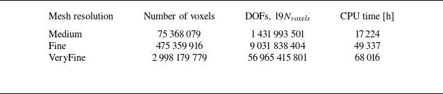
Grid convergence study for the impedance as function of the source frequency (a) acoustic resistance and (b) reactance for the three grid resolutions compared with experimental results by Jones et al. (Reference Jones, Watson, Parrott and Smith2004) at $M=0$
. The results are scaled with the liner porosity,
$M=0$
. The results are scaled with the liner porosity, $\sigma$
, for comparison.
$\sigma$
, for comparison.

A.4. Impedance validation
The grid convergence is verified also for the impedance for the simulations without flow at the three frequencies at a fixed SPL = 130 dB. The computed impedance is compared with experimental data obtained at the GFIT facility (GIT-95M test section) (Jones et al. Reference Jones, Watson, Parrott and Smith2004), where impedance was extracted using a two-dimensional finite element method (2-D-FEM). In the present numerical framework, the acoustic impedance is evaluated using the in situ technique, originally introduced by Dean (Reference Dean1974), which relies on pressure measurements acquired at two distinct locations within the liner: at the face sheet and at the backplate of the cavity. This method, often referred to as the two-microphone approach, provides a local estimation of impedance and is applicable under the assumptions that: (i) the acoustic wavelength is significantly larger than the cavity width; (ii) the cavity behaves as a locally reactive element due to sufficiently thick side walls; and (iii) acoustic waves entering the cavity are fully reflected at the backplate. This method is particularly suited to the current study, as only a single cavity is simulated.
Time-resolved pressure signals are sampled at discrete locations to reconstruct the transfer function between face sheet and backplate. Specifically, pressure at the face sheet is recorded every $30^\circ$
along a circular contour of radius 1
$30^\circ$
along a circular contour of radius 1 $d$
centred on each orifice, while the backplate pressure is sampled at the orifice centres. The resulting transfer functions are then averaged across all spatial locations to improve robustness. The impedance values are finally averaged out of the
$d$
centred on each orifice, while the backplate pressure is sampled at the orifice centres. The resulting transfer functions are then averaged across all spatial locations to improve robustness. The impedance values are finally averaged out of the $7$
orifices.
$7$
orifices.
Following the formulation by Dean (Reference Dean1974), Manjunath et al. (Reference Manjunath, Avallone, Casalino, Ragni and Snellen2018) and Avallone et al. (Reference Avallone, Manjunath, Ragni and Casalino2019), the normalised acoustic impedance $Z_f$
is obtained via:
$Z_f$
is obtained via:
 \begin{align} Z_{f} = \frac {Z}{Z_0} = -i \tilde {H}_{fb} \frac {1}{\sin (kd_c)}, \end{align}
where $Z_0$
is the characteristic impedance of air,
$Z_0$
is the characteristic impedance of air,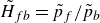 $\tilde {H}_{fb} = \tilde {p}_{f} / \tilde {p}_{b}$
is the complex pressure transfer function between face sheet and backplate,
$\tilde {H}_{fb} = \tilde {p}_{f} / \tilde {p}_{b}$
is the complex pressure transfer function between face sheet and backplate, $d_c$
is the cavity depth, and
$d_c$
is the cavity depth, and $k = \omega / c_0$
is the acoustic wavenumber, with
$k = \omega / c_0$
is the acoustic wavenumber, with $\omega$
the angular frequency and
$\omega$
the angular frequency and $c_0$
the speed of sound.
$c_0$
the speed of sound.
Surface data for the estimation of the impedance are sampled at a frequency of $20$
kHz. The flow field is, however, sampled such to have
$20$
kHz. The flow field is, however, sampled such to have $720$
point per wavelength. For each configurations, acoustic waves with
$720$
point per wavelength. For each configurations, acoustic waves with $10$
acoustic periods are considered based on the findings from previous studies by Manjunath et al. (Reference Manjunath, Avallone, Casalino, Ragni and Snellen2018), Avallone et al. (Reference Avallone, Manjunath, Ragni and Casalino2019) and DNS results by Zhang & Bodony (Reference Zhang and Bodony2016b
). Data are sampled after convergence of the unsteady field, which is in general obtained after no more than
$10$
acoustic periods are considered based on the findings from previous studies by Manjunath et al. (Reference Manjunath, Avallone, Casalino, Ragni and Snellen2018), Avallone et al. (Reference Avallone, Manjunath, Ragni and Casalino2019) and DNS results by Zhang & Bodony (Reference Zhang and Bodony2016b
). Data are sampled after convergence of the unsteady field, which is in general obtained after no more than $2$
acoustic periods.
$2$
acoustic periods.
The two components of the impedance, the resistance, $\text{Re[$Z_f$]}$
, and the reactance,
$\text{Re[$Z_f$]}$
, and the reactance, $\text{Im[$Z_f$]}$
, are shown in figure 29(a, b); they are both scaled with the porosity,
$\text{Im[$Z_f$]}$
, are shown in figure 29(a, b); they are both scaled with the porosity, $\sigma$
, to allow comparison with the reference experiments in the absence of grazing flow. As for the turbulent boundary layer, the case with resolution equal to
$\sigma$
, to allow comparison with the reference experiments in the absence of grazing flow. As for the turbulent boundary layer, the case with resolution equal to $40$
voxels
$40$
voxels $d$
-1 shows converging results and good agreement with the experimental results. The stronger dependence of the acoustic resistance on grid resolution is primarily due to the fact that the grazing flow modifies mainly the resistive part of the impedance, whereas the reactive part is largely controlled by the resonator geometry, i.e. height. In particular, refining the mesh near the wall improves the resolution within the boundary layer and the near-orifice flow field, which directly affects the resistance. This behaviour can be interpreted in two complementary ways. First, following the theoretical derivation by Panton & Miller (Reference Panton and Miller1975), a Helmholtz resonator can be modelled as a mass–spring–damper system. In that framework, the liner reactance is dominated by the term
$d$
-1 shows converging results and good agreement with the experimental results. The stronger dependence of the acoustic resistance on grid resolution is primarily due to the fact that the grazing flow modifies mainly the resistive part of the impedance, whereas the reactive part is largely controlled by the resonator geometry, i.e. height. In particular, refining the mesh near the wall improves the resolution within the boundary layer and the near-orifice flow field, which directly affects the resistance. This behaviour can be interpreted in two complementary ways. First, following the theoretical derivation by Panton & Miller (Reference Panton and Miller1975), a Helmholtz resonator can be modelled as a mass–spring–damper system. In that framework, the liner reactance is dominated by the term $\cot (k d_c)$
(with
$\cot (k d_c)$
(with $k$
the acoustic wavenumber and
$k$
the acoustic wavenumber and $d_c$
the cavity depth), while grazing-flow effects enter mainly through secondary terms (e.g. via orifice end corrections). Second, consistent with the semi-empirical model of Yu et al. (Reference Yu, Ruiz and Kwan2008), the reactance depends predominantly on SPL and geometry, whereas grazing flow primarily influences the end-correction and resistive terms, hence affecting the resistance more strongly than the reactance (Paduano et al. Reference Paduano, Scarano, Bonomo, Casalino, Cordioli and Avallone2026a
).
$d_c$
the cavity depth), while grazing-flow effects enter mainly through secondary terms (e.g. via orifice end corrections). Second, consistent with the semi-empirical model of Yu et al. (Reference Yu, Ruiz and Kwan2008), the reactance depends predominantly on SPL and geometry, whereas grazing flow primarily influences the end-correction and resistive terms, hence affecting the resistance more strongly than the reactance (Paduano et al. Reference Paduano, Scarano, Bonomo, Casalino, Cordioli and Avallone2026a
).
A.5. Impedance as function of SPL
In figure 30, the impedance for the cases with ( ${M}\!=\!0.3$
) and without (
${M}\!=\!0.3$
) and without ( ${M}\!=\!0$
) grazing turbulent flow for varying SPL of the grazing acoustic wave at a frequency of
${M}\!=\!0$
) grazing turbulent flow for varying SPL of the grazing acoustic wave at a frequency of $2200$
Hz are compared. The two components of the acoustic impedance, resistance and reactance, averaged out of the
$2200$
Hz are compared. The two components of the acoustic impedance, resistance and reactance, averaged out of the $7$
orifices and scaled by the liner porosity
$7$
orifices and scaled by the liner porosity $\sigma$
, are plotted.
$\sigma$
, are plotted.
(a) Resistance and (b) reactance components of impedance scaled with the liner porosity $\sigma$
. The frequency of the acoustic wave is 2200 Hz, while the amplitude varies between 130 and 160 dB.
$\sigma$
. The frequency of the acoustic wave is 2200 Hz, while the amplitude varies between 130 and 160 dB.

The results show that, with increasing SPL, the resistance grows more significantly in the absence of flow compared with the case with grazing turbulent flow. Specifically, while the resistance exhibits an exponential increase without flow, it remains nearly constant up to $150$
dB in the presence of flow, only starting to increase at higher SPL. Additionally, it is observed that, in the presence of grazing flow, the amplitude of the resistance is comparable to the maximum value attained in the no-flow case. The grazing flow also affects the reactance: for
$150$
dB in the presence of flow, only starting to increase at higher SPL. Additionally, it is observed that, in the presence of grazing flow, the amplitude of the resistance is comparable to the maximum value attained in the no-flow case. The grazing flow also affects the reactance: for ${M}\!=\!0$
, it decreases with increasing SPL, whereas for
${M}\!=\!0$
, it decreases with increasing SPL, whereas for ${M}\!=\!0.3$
, it slightly increases with SPL. These results clearly demonstrate that the acoustic impedance is significantly altered by the presence of a grazing turbulent flow. This behaviour may be related to modifications in the acoustic-induced flow topology and the associated dissipation mechanisms.
${M}\!=\!0.3$
, it slightly increases with SPL. These results clearly demonstrate that the acoustic impedance is significantly altered by the presence of a grazing turbulent flow. This behaviour may be related to modifications in the acoustic-induced flow topology and the associated dissipation mechanisms.
Appendix B. Evaluation of the impinging acoustic energy
The acoustic power used to normalise the dissipation terms in figures 16 and 18 is computed by integrating the fluctuating pressure field along the entire domain height, as illustrated in figure 31. This differs from the definition adopted by Tam & Kurbatskii (Reference Tam and Kurbatskii2000), where the orifice surface was used as the reference dimension.
Methodology for evaluating the impinging acoustic energy $E_{{i}}$
(W m−1) and downstream energy
$E_{{i}}$
(W m−1) and downstream energy $E_{{out}}$
along the domain height. Energy distributions in (dB) are reported for (a, b) SPL = 130 dB without and with grazing flow, and (c, d) SPL = 150 dB.
$E_{{out}}$
along the domain height. Energy distributions in (dB) are reported for (a, b) SPL = 130 dB without and with grazing flow, and (c, d) SPL = 150 dB.

In the two-dimensional configuration, the acoustic pressure associated with the incident wave varies along the wall-normal direction. Denoting by $\hat {p}_i(y)$
the incident pressure amplitude at a given wall-normal location
$\hat {p}_i(y)$
the incident pressure amplitude at a given wall-normal location $y$
, the local time-averaged acoustic intensity of a harmonic plane wave is evaluated as
$y$
, the local time-averaged acoustic intensity of a harmonic plane wave is evaluated as
 \begin{align} \overline {I}_i(y) = \frac {\hat {p}_i^{\,2}(y)}{2\rho c}, \end{align}
where $\rho$
is the fluid density and
$\rho$
is the fluid density and $c$
is the speed of sound. The impinging acoustic quantity denoted
$c$
is the speed of sound. The impinging acoustic quantity denoted $E_{\text{i}}$
is then obtained by integrating the local acoustic intensity along the wall-normal direction on an upstream control plane normal to the streamwise direction,
$E_{\text{i}}$
is then obtained by integrating the local acoustic intensity along the wall-normal direction on an upstream control plane normal to the streamwise direction,
 \begin{align} E_{\text{i}} = \int _{0}^{h_c} \overline {I}_i(y)\,\mathrm{d}y = \int _{0}^{h_c} \frac {\hat {p}_i^{\,2}(y)}{2\rho c}\,\mathrm{d}y. \end{align}
This quantity has units of $\mathrm{W\,m^{-1}}$
and represents the time-averaged acoustic power per unit span, i.e. an acoustic energy flux per unit time and per unit span. For the three-dimensional evaluation, the corresponding impinging acoustic power is obtained by multiplying this value by the spanwise extent of the 3-D computational domain, yielding the total impinging acoustic power in
$\mathrm{W\,m^{-1}}$
and represents the time-averaged acoustic power per unit span, i.e. an acoustic energy flux per unit time and per unit span. For the three-dimensional evaluation, the corresponding impinging acoustic power is obtained by multiplying this value by the spanwise extent of the 3-D computational domain, yielding the total impinging acoustic power in $\mathrm{W}$
. This three-dimensional value is used to normalise the dissipation terms reported in figures 16 and 18, as well as in the full 3-D analysis.
$\mathrm{W}$
. This three-dimensional value is used to normalise the dissipation terms reported in figures 16 and 18, as well as in the full 3-D analysis.
The same formulation can be applied on a downstream control plane to evaluate the transmitted acoustic power $E_{{out}}$
. With this definition, the impinging power
$E_{{out}}$
. With this definition, the impinging power $E_{{i}}$
upstream of the orifice and the outgoing
$E_{{i}}$
upstream of the orifice and the outgoing $E_{{out}}$
downstream of the orifice can be consistently compared to highlight the modification of the pressure field due to the presence of the orifice. Shifting the evaluation planes within two orifice diameters upstream or downstream does not affect the results, confirming the robustness of the method.
$E_{{out}}$
downstream of the orifice can be consistently compared to highlight the modification of the pressure field due to the presence of the orifice. Shifting the evaluation planes within two orifice diameters upstream or downstream does not affect the results, confirming the robustness of the method.
Representative wall-normal profiles of the pressure fluctuation amplitude (normalised with the reference pressure and reported in dB) are shown in figure 31 for SPL $=130$
and
$=130$
and $150$
dB for the sake of conciseness. In the absence of grazing flow (panels a, c), the distribution resembles an acoustic boundary layer: energy peaks at the domain centreline and decreases towards the wall. Downstream of the orifice, the profiles exhibit the expected attenuation due to dissipation.
$150$
dB for the sake of conciseness. In the absence of grazing flow (panels a, c), the distribution resembles an acoustic boundary layer: energy peaks at the domain centreline and decreases towards the wall. Downstream of the orifice, the profiles exhibit the expected attenuation due to dissipation.
When a grazing flow is introduced at 130 dB (panel b), the profiles are markedly altered. The acoustic energy increases towards the wall, reflecting the contribution of turbulence-induced pressure fluctuations in the boundary layer. Downstream of the orifice, the energy decreases at the centre of the domain, but slightly increases near the wall due to the interaction of the shear layer with the orifice jet.
At 150 dB with grazing flow (panel d), the profiles more closely resemble the no-flow case: the acoustic source dominates over the background turbulence, yielding a higher acoustic-to-aerodynamic fluctuation ratio, in agreement with Scarano et al. (Reference Scarano, Lyu, Paduano and Avallone2026). Interestingly, downstream of the orifice, the energy distribution exhibits a local maximum not at the wall but at $y/h_c \approx -0.1$
, suggesting that the stronger jetting effect at this SPL penetrates deeper into the grazing flow and locally amplifies the pressure fluctuations.
$y/h_c \approx -0.1$
, suggesting that the stronger jetting effect at this SPL penetrates deeper into the grazing flow and locally amplifies the pressure fluctuations.
Appendix C. Acoustic-induced velocity normalised with respect to the lumped element model of the Helmholtz resonator
Spatial distribution along the diameter at half-face-sheet thickness of the non-dimensional acoustic-induced vertical velocity normalised with the lumped element velocity. Thicker lines represent larger SPL values. Inflow and outflow phases are reported.

(a) 3-D region where the shear stress is integrated close to the orifice internal wall, (b) iso-surface $\varPhi ^+=0.1$
of the stress tensor at M = 0 from another perspective.
$\varPhi ^+=0.1$
of the stress tensor at M = 0 from another perspective.

To give additional confidence that the wall-modelled LB–VLES framework correctly reproduces both the order of magnitude and the peak value of the acoustic-induced velocity, the profiles at the centre of the orifice for the no-flow case are normalised with respect to the lumped element model of the Helmholtz resonator (Morse & Ingard Reference Morse and Ingard1968):
 \begin{align} v^*_{ac} = \frac {\hat {p}}{\rho \omega (\tau +0.8d)} \frac {1}{\sqrt { \left [(\omega _H/\omega )^2 - 1 \right ]^2 + (\omega _H/\omega Q)^2 }}, \end{align}
where $\hat {p}$
is the pressure fluctuation amplitude,
$\hat {p}$
is the pressure fluctuation amplitude, $\omega$
and
$\omega$
and $\omega _H$
are the forcing and resonant frequencies,
$\omega _H$
are the forcing and resonant frequencies, $Q$
is the quality factor (taken as
$Q$
is the quality factor (taken as $10$
),
$10$
), $\rho$
is the density, and
$\rho$
is the density, and $d$
and
$d$
and $\tau$
are the diameter and thickness of the orifice, respectively. This expression gives theoretical peak velocities for Helmholtz resonator in the absence of grazing flow. The values obtained are
$\tau$
are the diameter and thickness of the orifice, respectively. This expression gives theoretical peak velocities for Helmholtz resonator in the absence of grazing flow. The values obtained are $3.6$
,
$3.6$
, $9.5$
,
$9.5$
, $30.2$
and
$30.2$
and $67.6\,\mathrm{m\,s}^{-1}$
for the four tested SPLs.
$67.6\,\mathrm{m\,s}^{-1}$
for the four tested SPLs.
The normalised acoustic velocity, reported in figure 32, is observed to approach unity across the investigated SPL range, indicating that the numerical framework accurately captures the expected oscillatory velocity amplitude inside the orifice. This agreement provides additional confidence that the wall model correctly predicts the near-wall gradients associated with the acoustic motion within the orifice.
Appendix D. Integration region for viscous dissipation
The integration region used for the viscous dissipation in 3-D is illustrated in figure 33 (a). In the three-dimensional formulation, this region forms a toroidal volume surrounding the internal wall of the orifice, corresponding to a near-wall band where viscous stresses are dominant (figure 33 b).

 y
y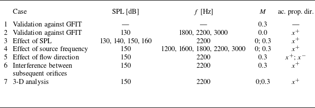
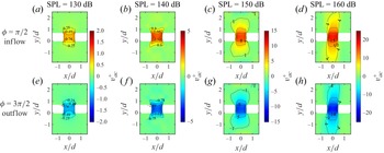
 vac+
vac+ ϕ=π/2
ϕ=π/2 ϕ=3π/2
 vac+
vac+ ϕ=π/2
ϕ=π/2 ϕ=3π/2
 M=0.3
M=0.3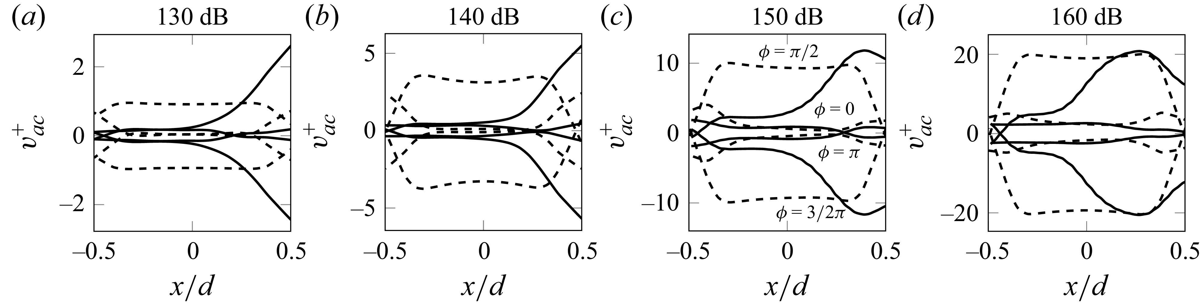
 vac+
vac+ M=0.3
M=0.3
 M=0.3
M=0.3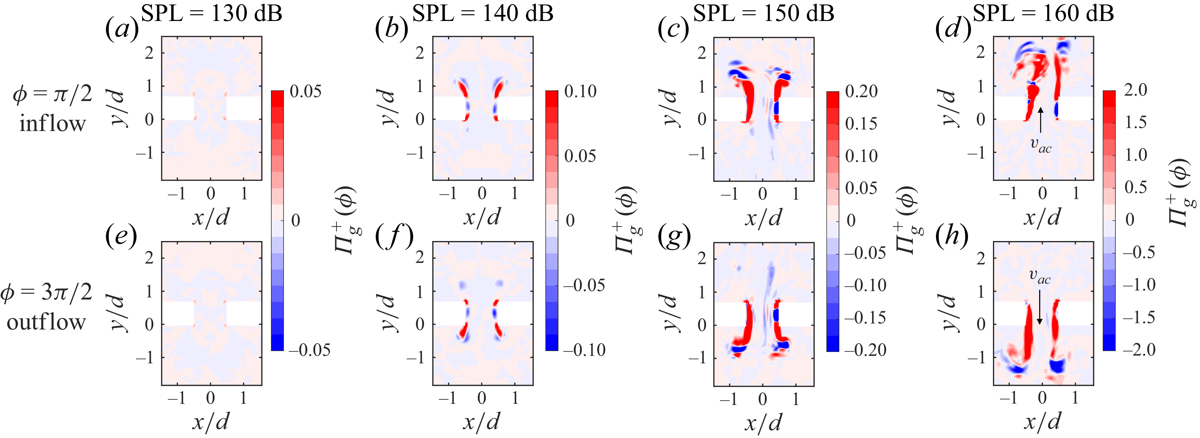
 Πg+
Πg+
 Πg+
Πg+ M=0.3
M=0.3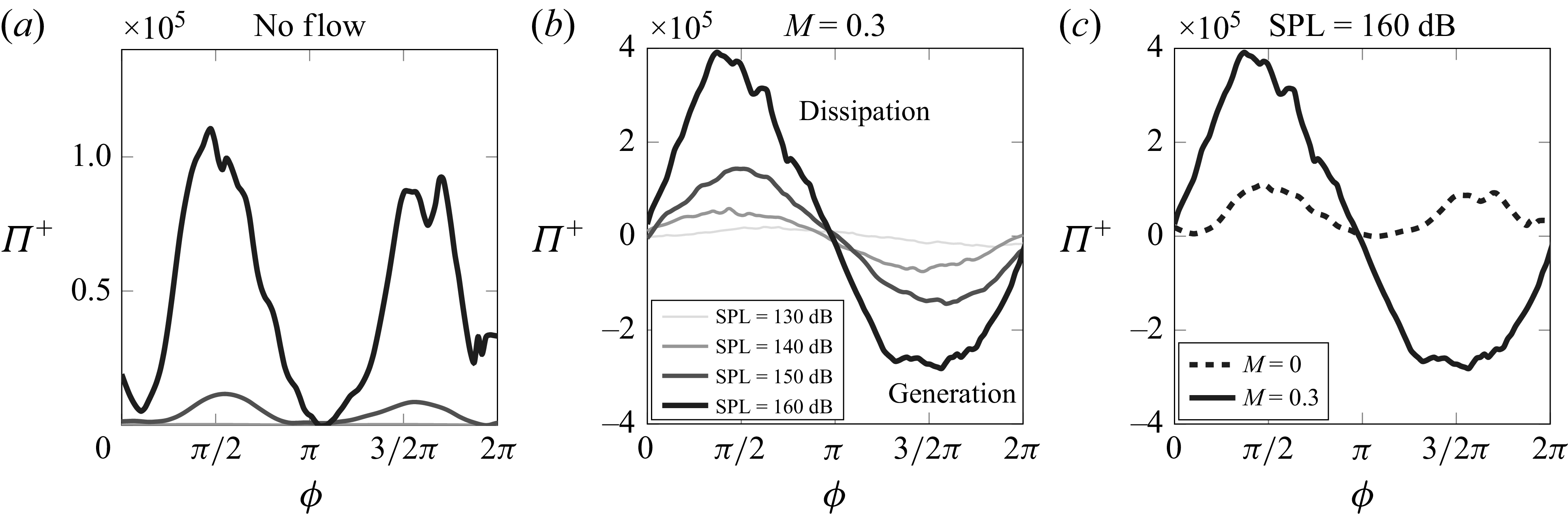
 Π+(ϕ)
Π+(ϕ) M=0.3
M=0.3 M=0.3
M=0.3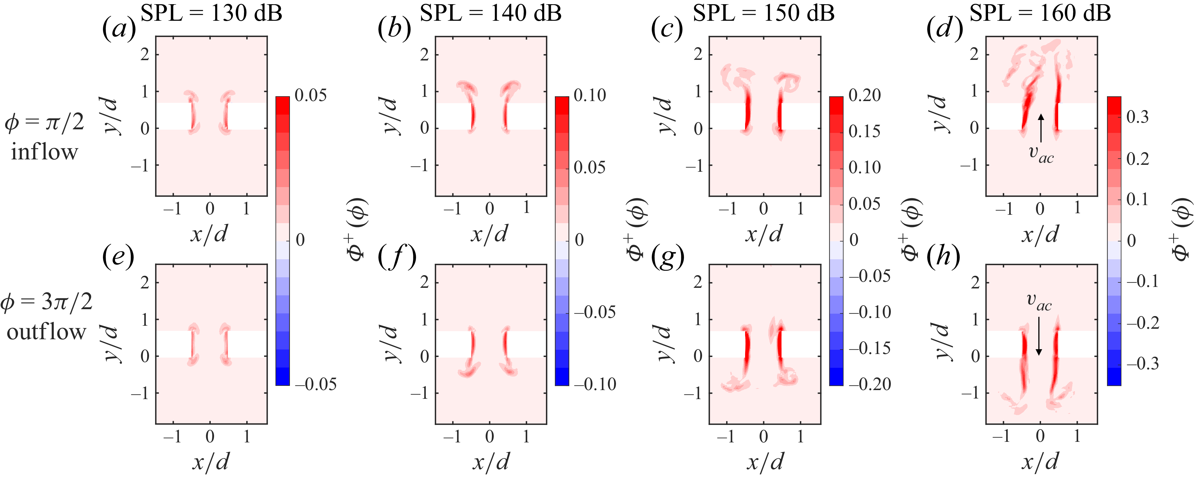
 Φ+
Φ+ M=0
M=0
 D+
D+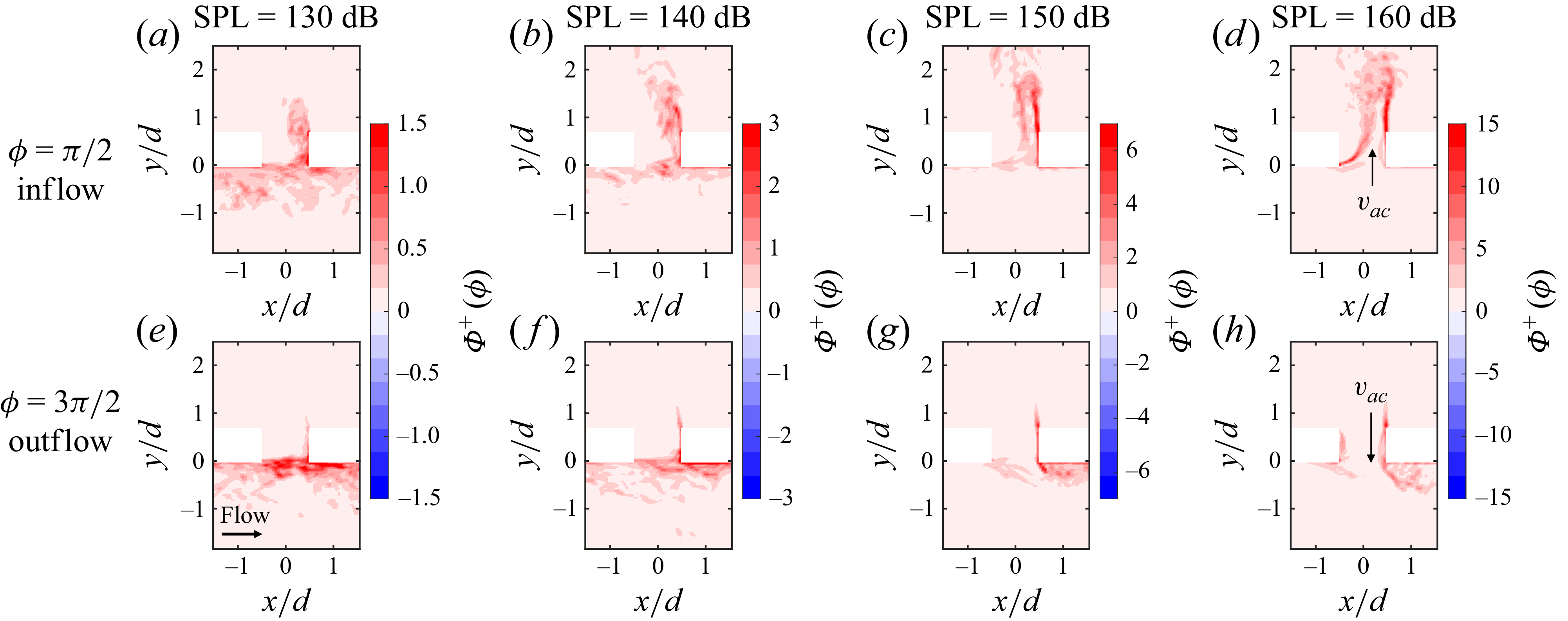
 Φ+
Φ+ M=0.3
M=0.3
 D+
D+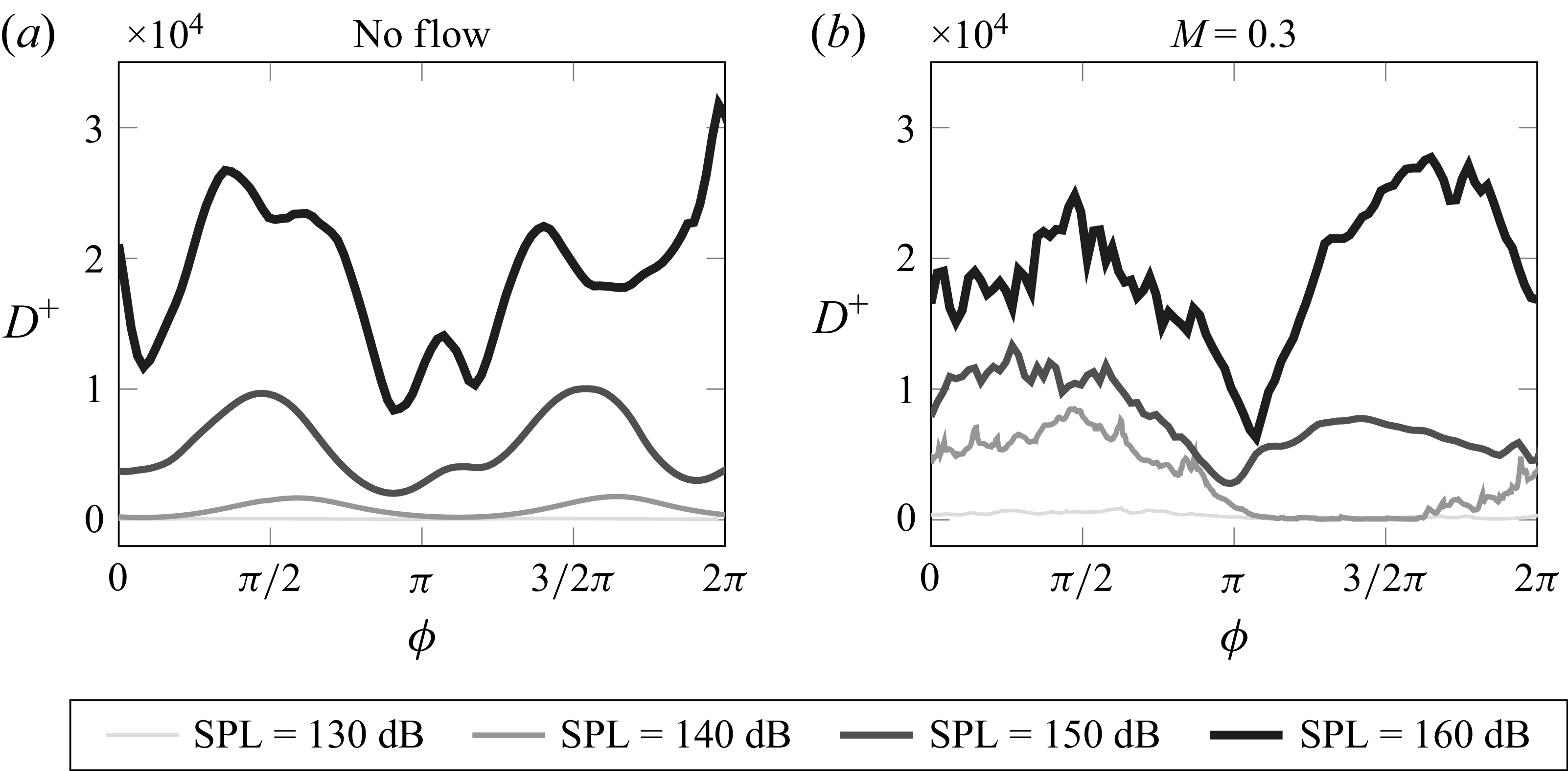
 D+
D+
 Πg+=±0.1
 Φ+=0.06
 Π+
Π+ D+
D+
 Πg+=±5
 Φ+=0.1
 Π+
Π+ D+
D+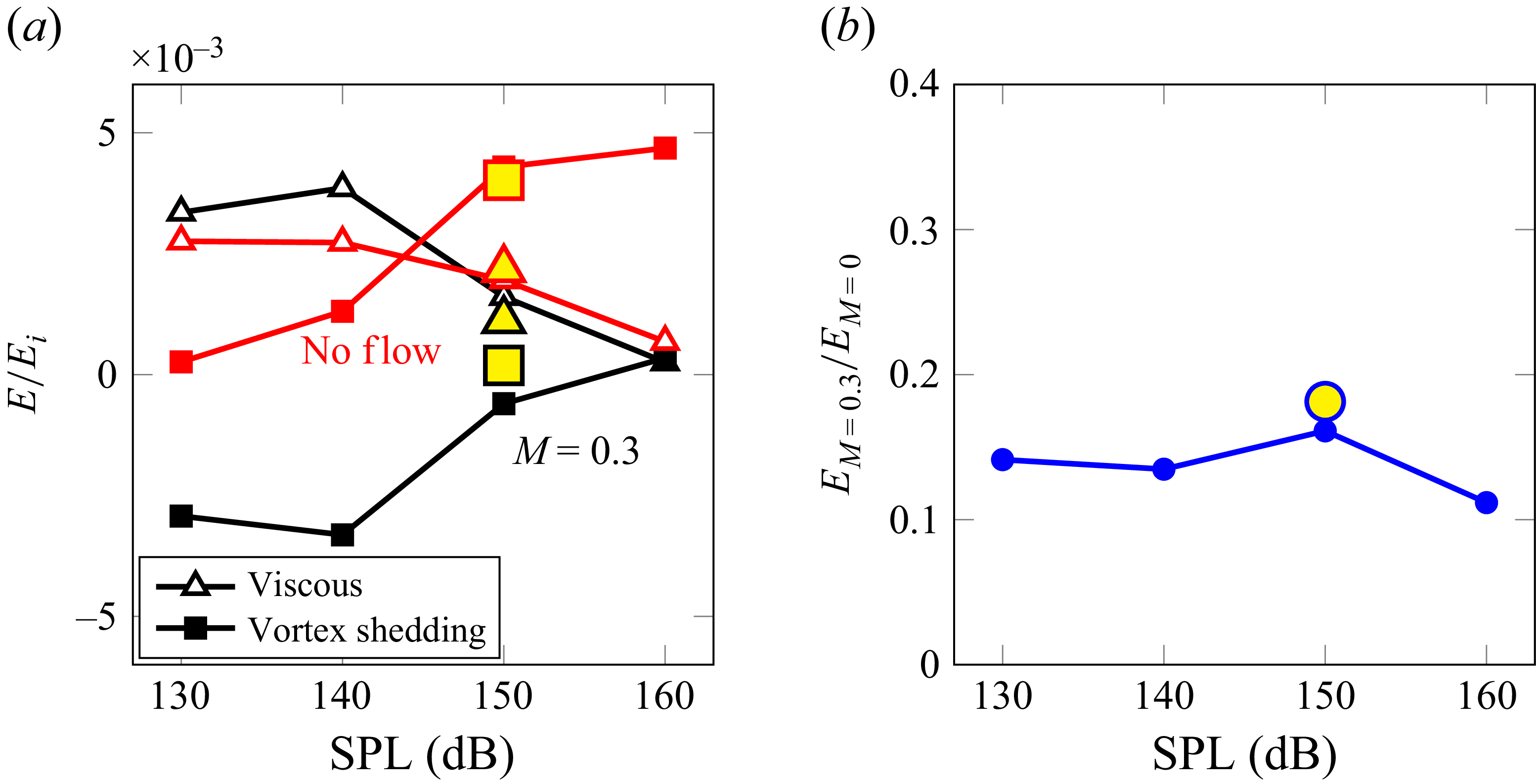

 Π+(ϕ)
Π+(ϕ) D+(ϕ)
D+(ϕ) M=0.3
M=0.3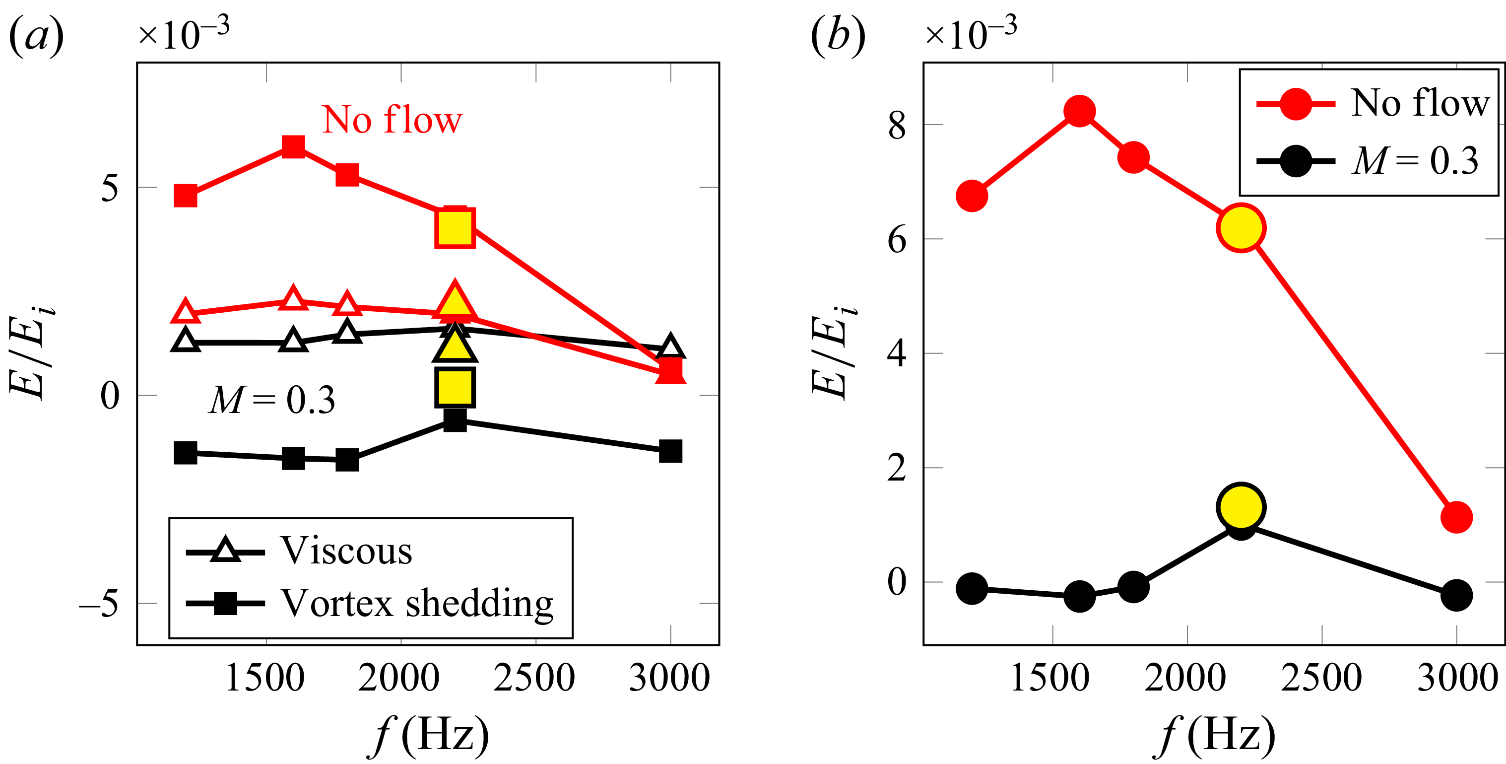

 M=0.3
M=0.3 y/d=0
y/d=0 Π+(ϕ)
Π+(ϕ) D+(ϕ)
D+(ϕ) x+
x+
 M=0.3
M=0.3 y/lc=0
 vac+
vac+ ϕ=π/2
ϕ=π/2 ϕ=3π/2
 M=0.3
M=0.3
 Πg+
Πg+ M=0.3
M=0.3 Π+(ϕ)
Π+(ϕ)
 M=0.3
M=0.3 D+(ϕ)
D+(ϕ)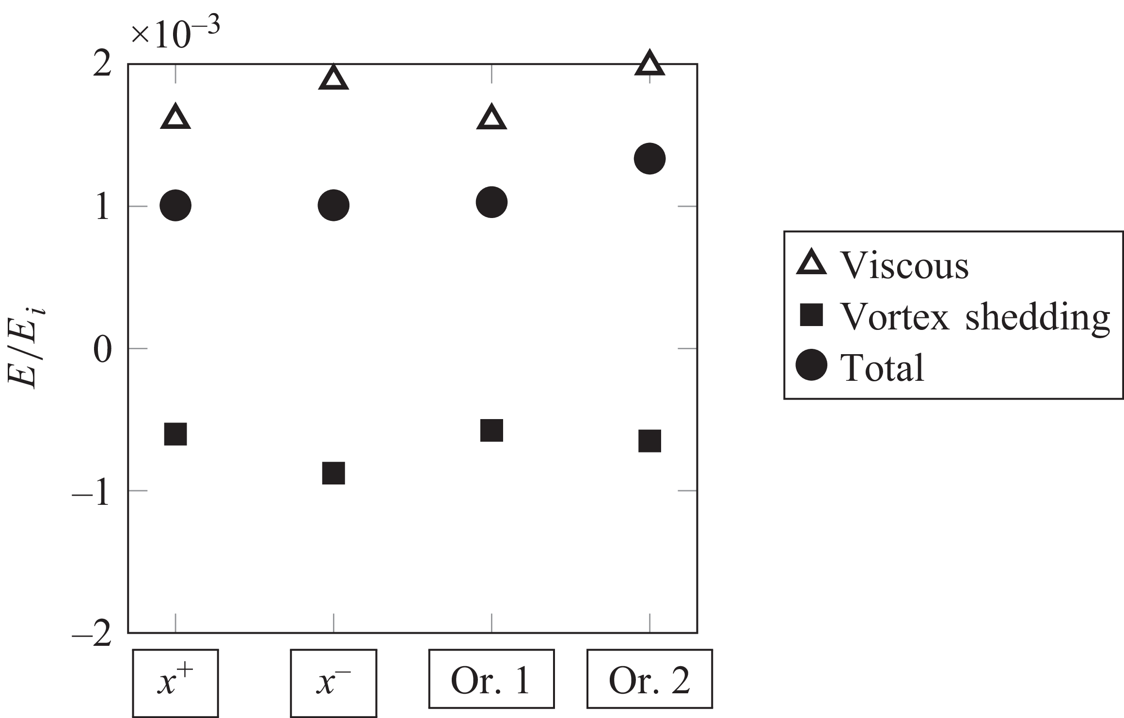
 M=0.3
M=0.3 x+
x+ x−
x−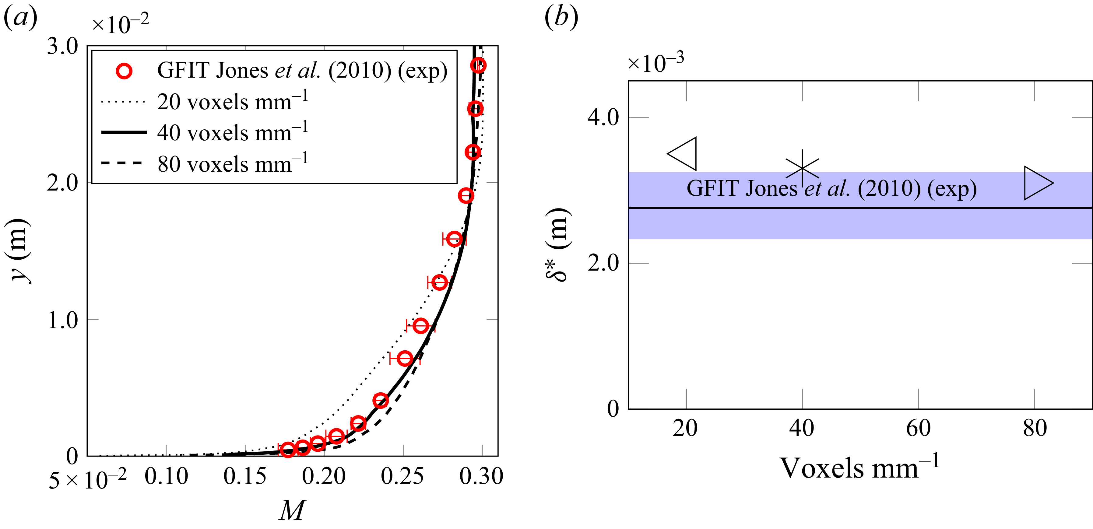

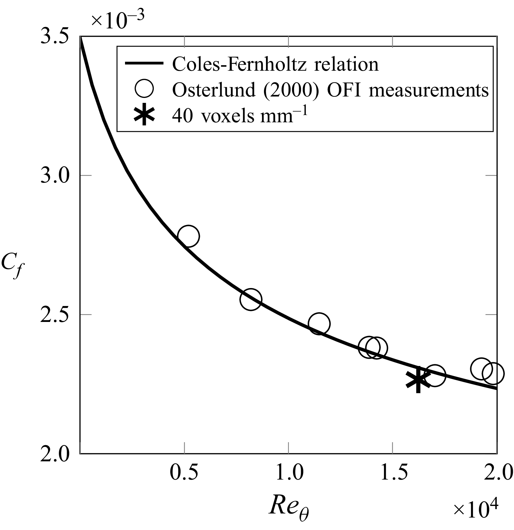
 Reθ
Reθ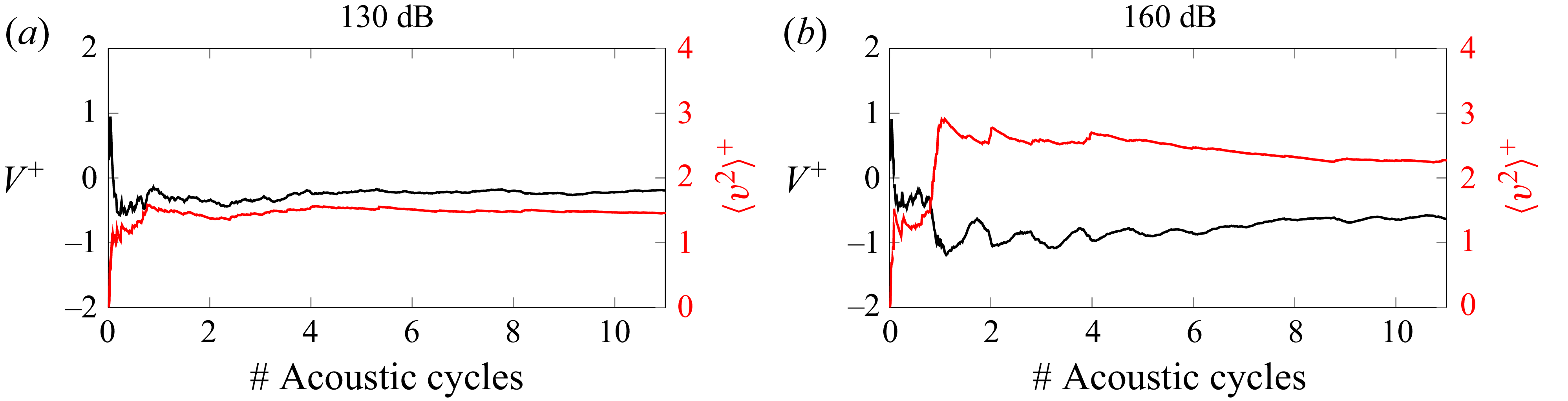
 y+≅250
 (y/d≅−0.9)
 M=0.3
M=0.3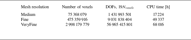
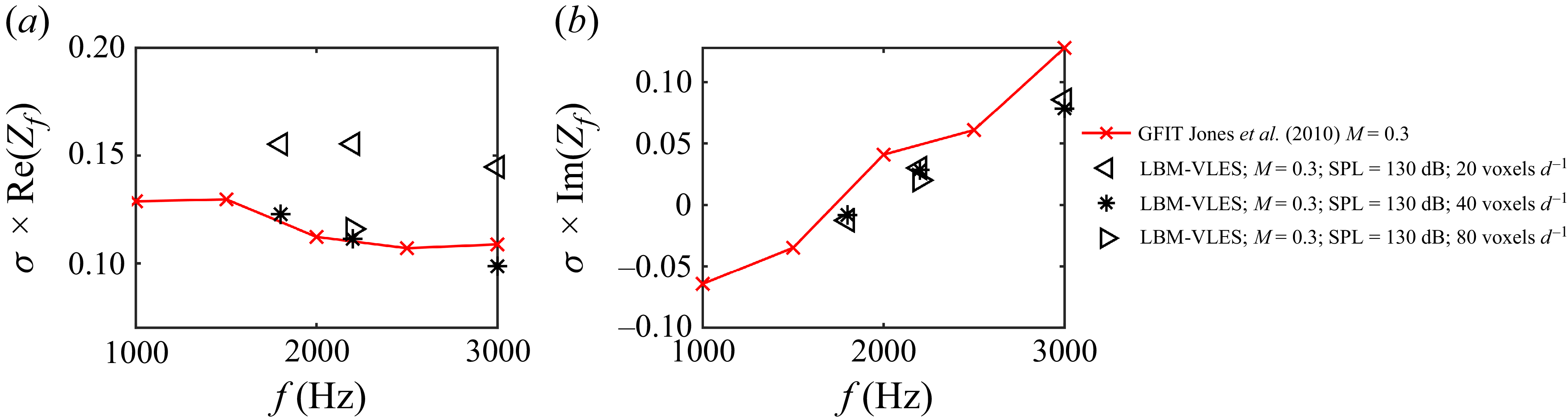
 M=0
M=0 σ
σ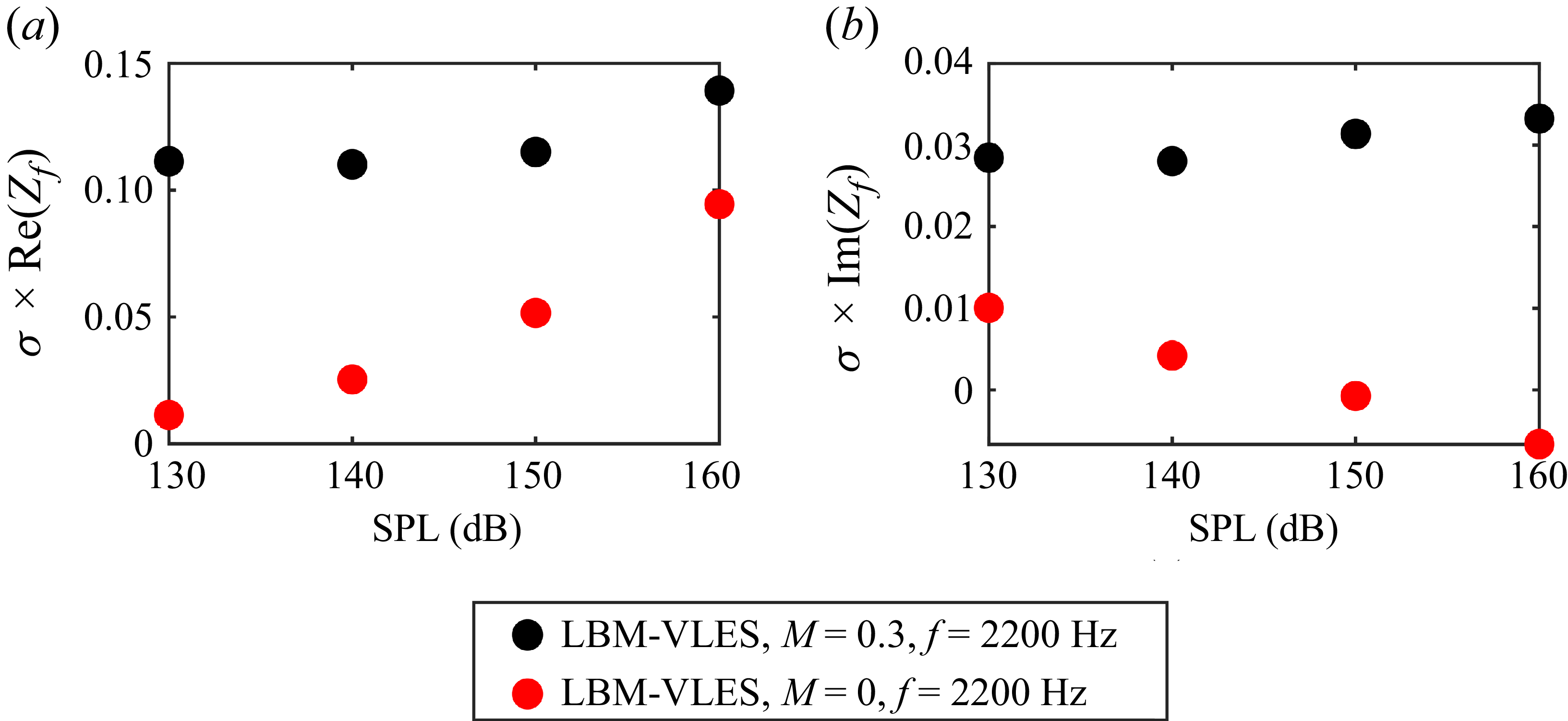
 σ
σ
 Ei
Ei Eout
Eout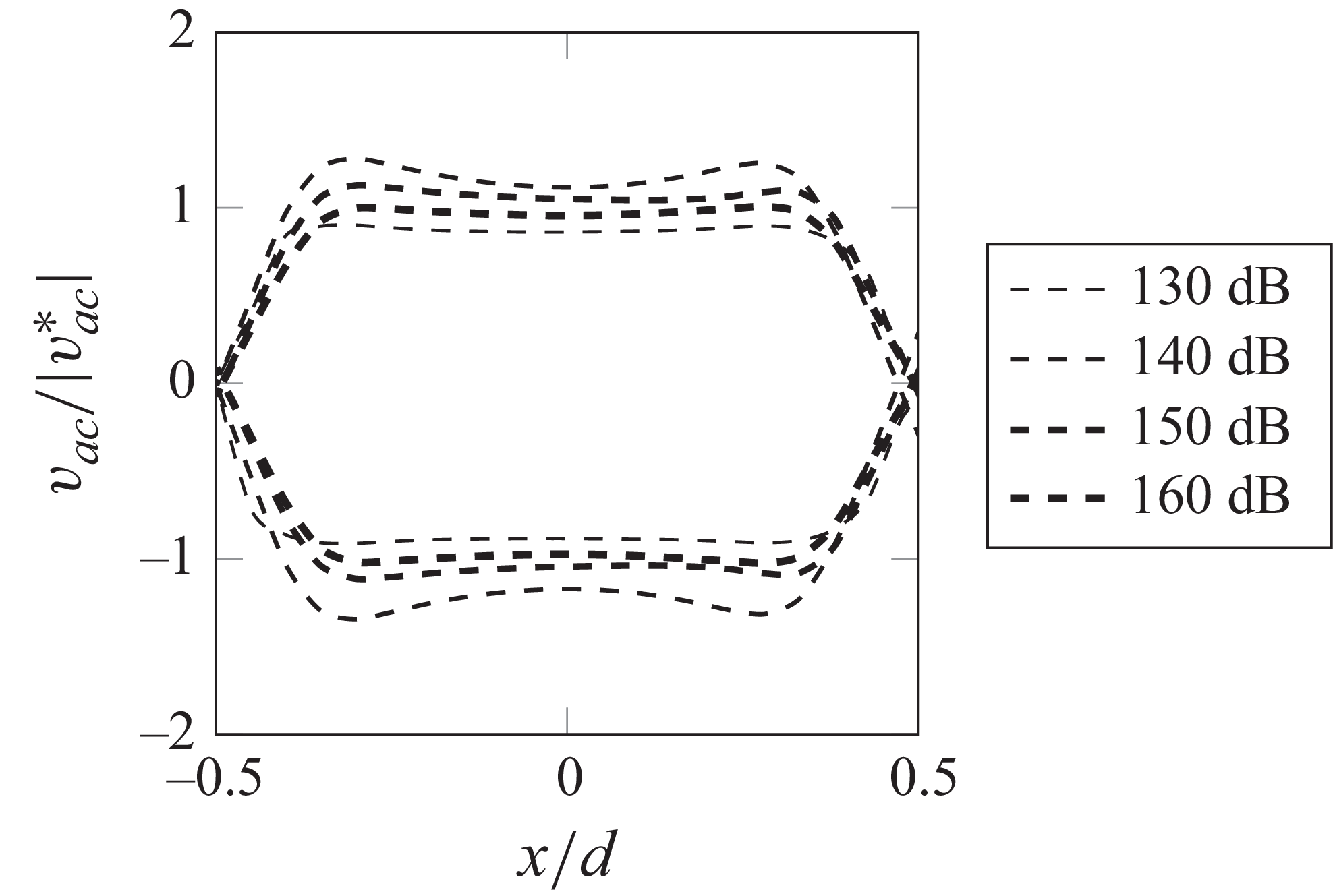

 Φ+=0.1
 Open access

