


1. Introduction
Kinetic plasma physics is described, typically, using various formulations or realizations of Boltzmann-like transport equations for the electron and ion species. A special case that is frequently studied is that of the dynamics restricted to one spatial dimension and one momentum dimension (‘1D-1V’) for a single species of particles, given by

where the normalized electric field is given by solving $\boldsymbol {\nabla } \boldsymbol {\cdot } \tilde {E} = 1 - \int \tilde {f}\,{\rm d}\tilde {v}$ , and the normalized particle distribution function is $\tilde {f} = f(t,x,v) / n_e v_{{\rm th}}^3$
 . The quantities are normalized to electrostatic units where $\tilde {v} = v / v_{{\rm th}}, \tilde {x} = x/\lambda _D, \tilde {t} = \omega _p t, \tilde {m} = m/m_e$
 and $\tilde {E} = e E / m_e v_{{\rm th}} \omega _p$
 . Here, $v_{{\rm th}}$
 is the thermal velocity, $\omega _p$
 is the plasma frequency, $\lambda_D$
 is the Debye length, and $m_e$
 , and $e$
 , are the electron mass, and charge, respectively.
The left-hand side of this equation describes the evolution of the particle distribution in ‘macroscopic’ field $E$ that arises self-consistently from the one-particle distribution $f$
 . The right-hand side provides a description of two-particle and higher correlations (i.e. collisions). Equation (1.1), along with Gauss's law and with a particular form of the collision operator for two-particle interactions, is often termed the Vlasov–Poisson–Fokker–Planck (VPFP) equation set. Solving the VPFP set is often analytically intractable, even in 1D-1V. This is because the left-hand side has a stiff linear transport term, has a nonlinear term in $E \partial f/\partial v$
 and can sustain wave propagation and other hyperbolic partial-differential equation (PDE) behaviour. Additionally, the right-hand side is typically represented by a hyperbolic advection–diffusion PDE. Making progress on kinetic plasma physics often requires computational simulation tools.
Numerical solutions to the 1D-1V VPFP equation set have been applied in research on laser–plasma interactions in the context of inertial fusion, for example in plasma-based accelerators (Krall, Joyce & Esarey Reference Krall, Joyce and Esarey1991; Thomas Reference Thomas2016), space physics (Chen, Klein & Howes Reference Chen, Klein and Howes2019), fundamental plasma physics (Pezzi et al. Reference Pezzi, Cozzani, Califano, Valentini, Guarrasi, Camporeale, Brunetti, Retinó and Veltri2019) and inertial fusion (Strozzi et al. Reference Strozzi, Williams, Langdon and Bers2007; Fahlen et al. Reference Fahlen, Winjum, Grismayer and Mori2009; Banks et al. Reference Banks, Berger, Brunner, Cohen and Hittinger2011). Such numerical simulations may be used to explore initial conditions and forcing functions to understand the behaviour of a physical effect in response to input parameters. Multi-dimensional ‘brute-force’ scans are, however, inefficient and costly and it is therefore beneficial to seek a more guided approach by leveraging optimization techniques.
Optimization techniques can be grouped into gradient-based or gradient-free methods. Gradient-free methods are typically useful when it is not practical to obtain the gradient of the desired objective function (Nocedal & Wright Reference Nocedal and Wright2006). For example, when the objective function is the outcome of a plasma-based accelerator experiment. In this case, one can use classical approaches like the Nelder–Mead algorithm (Shalloo et al. Reference Shalloo, Dann, Gruse, Underwood, Antoine, Arran, Backhouse, Baird, Balcazar and Bourgeois2020) or more modern alternatives like Bayesian (Shalloo et al. Reference Shalloo, Dann, Gruse, Underwood, Antoine, Arran, Backhouse, Baird, Balcazar and Bourgeois2020; Jalas et al. Reference Jalas, Kirchen, Messner, Winkler, Hübner, Dirkwinkel, Schnepp, Lehe and Maier2021) or evolutionary (He et al. Reference He, Hou, Lebailly, Nees, Krushelnick and Thomas2015; Smith et al. Reference Smith, Orban, Morrison, George, Ngirmang, Chowdhury and Roquemore2020) algorithms. These algorithms have been shown to be effective in the small $N_p$ regime, where $N_p$
 is the number of parameters to optimize. While there has been some success in using gradient-free approaches in large $N_p$
 regimes e.g. in reinforcement learning scenarios (Salimans et al. Reference Salimans, Ho, Chen, Sidor and Sutskever2017), it has been when the gradient information is unreliable. In general, as $N_p \gg 1$
 , utilizing gradient-free methods becomes computationally intractable or unstable. In the work here, we learn functions reparametrized via a neural network, and therefore we seek the optimal neural network weights and biases. In this work, $\mathcal {O}(10) \leq N_p \leq \mathcal {O}(10^3)$
 , and automatic-differentiation-driven, gradient-based methods offer significant advantages.
While not focused on the nonlinear kinetic plasma dynamics, recent works have applied gradient-based optimization to fusion device design. Analytic approaches have resulted in the development of adjoint methods for shape derivatives of functions that depend on magnetohydrodynamic equilibria (Antonsen, Paul & Landreman Reference Antonsen, Paul and Landreman2019; Paul et al. Reference Paul, Antonsen, Landreman and Cooper2020). These methods have been used to perform optimization of stellarator design (Paul, Landreman & Antonsen Reference Paul, Landreman and Antonsen2021). Other work uses gradients obtained from analytic (Zhu et al. Reference Zhu, Hudson, Song and Wan2017) and automatic differentiationFootnote 1 (AD) (McGreivy, Hudson & Zhu Reference McGreivy, Hudson and Zhu2021; Conlin et al. Reference Conlin, Dudt, Panici and Kolemen2022; Dudt et al. Reference Dudt, Conlin, Panici and Kolemen2022; Panici et al. Reference Panici, Conlin, Dudt and Kolemen2022) towards similar device optimization goals. Here, we propose the application of gradient-based optimization towards understanding the nonlinear, kinetic plasma dynamics using differentiable kinetic simulations.
Differentiable simulations have been used in a variety of contexts for such guided searches, for example, learning parameters for molecular dynamics (Schoenholz, Cubuk & Jax Reference Schoenholz, Cubuk and Jax2019), learning differencing stencils in PDEs (Bar-Sinai et al. Reference Bar-Sinai, Hoyer, Hickey and Brenner2019; Zhuang et al. Reference Zhuang, Kochkov, Bar-Sinai, Brenner and Hoyer2020; Kochkov et al. Reference Kochkov, Smith, Alieva, Wang, Brenner and Hoyer2021) and controlling PDEs (Holl, Koltun & Thuerey Reference Holl, Koltun and Thuerey2020). Here, we apply AD towards learning physical relationships and discovering novel phenomena in the VPFP dynamical system by training neural networks through differentiable simulations that solve (1.1).
In the rest of the manuscript, we first develop a conceptual framework for how one might implement gradient-descent-based optimization of parameters and learning of functions via differentiable programs. We then apply this framework towards kinetic plasma physics. Specifically, we extend the findings in Fahlen et al. (Reference Fahlen, Winjum, Grismayer and Mori2009) of the etching of nonlinear plasma wavepackets to study the effect of the hot electrons from one wavepacket on downstream wavepackets using a gradient-based approach. To do this, we train a neural network that provides control parameters to the PDE solver. By choosing physical parameters as inputs and control parameters as outputs of the neural network, we enable the neural network to learn a function that describes the physical relationship between the plasma parameters and the forcing function parameters e.g. the resonance frequency. We train the neural network in an unsupervised fashion using a cost function based on minimizing the free energy and maximizing the non-Maxwellian-ness of the plasma distribution function. This enables us to create self-learning plasma physics simulations, where the optimization process provides a physically interpretable function that can enable physics discovery.
2. Physics Discovery using Differentiable Simulations
In this section, we provide a step-by-step description of how a traditional simulation-based computational physics workflow may be modified to perform closed-loop optimization.
2.1. Open loop: manual workflow
Figure 1(a) depicts a typical simulation workflow represented as a cyclic graph. The user defines the parametric inputs that create the state vector $\boldsymbol {x}$ . This can contain any parameters that are used to define the simulation e.g. the grid size, the number of solver steps, etc. For didactic purposes, the physical parameters to the simulation may be separated from $\boldsymbol {x}$
 into a different vector of inputs $\boldsymbol {p_d}$
 e.g. the forcing function parameters, the viscosity coefficient etc.
(a) A typical workflow where the user provides the initial conditions and forcing function parameters to a PDE solve. The output of the solve is stored as the final state $\boldsymbol {x_f}$ . The final state is analysed using domain-specific postprocessing algorithms. (b) A cost function and a parameter scan are introduced which enables= a closed-loop search. (c) A gradient-descent-based optimization algorithm replaces the parameter scan to provide a more efficient search mechanism. This requires the components in the purple background to be written in an auto-differentiable framework. (d) We add a neural network that generates the forcing function parameters as a function of other parameters. This generalizes the learnings from (c) and enables a continuous representation within the learned parameters.

Each of $\boldsymbol {x}$ and $\boldsymbol {p_d}$
 is passed to the algorithm that solves the PDE which is represented by the function, $\mathcal {V}$
 . The output of these simulations is stored in the final state vector $\boldsymbol {x_f}$
 . The final state is postprocessed using a domain-specific set of algorithms devised by the user or otherwise. The results of the postprocessing are interpreted by the user who then determines the next set of inputs and parameters.
2.2. Closed loop: brute-force parameter scan
Figure 1(b) shows a more automated workflow. We replace the grey-box postprocessing step with the calculation of a scalar quantity $S$ using a cost function $\mathcal {C}$
 on the final state $\boldsymbol {x_f}$
 . This reduces the complexity of the interpretation of the postprocessing and enables a more rapid search in parameter space. The decrease in required human effort for completing one cycle enables the user to execute this loop as a brute-force parameter scan over a pre-defined parameter space. At the end, the user can look up the minimum/maximum of the scalar cost function, and find the parameters which provide that minimum.
The parameter scan approach scales with the number of different unique parameters and the number of values of each parameter. e.g. a two-dimensional search in $x$ and $y$
 requires $N_x \times N_y$
 calculations. Therefore, the parameter scan approach quickly becomes inefficient when there are many parameters to scan, or when the required resolution in parameter space is very high. To search this parameter space efficiently, and to escape the linear scaling with each parameter, we can use gradient descent.
2.3. Gradient-descent-based parameter learning
Figure 1(c) includes two modifications. The user/parameter search grey box has been replaced with a gradient-descent-based optimization algorithm. This algorithm provides the updated parameters, e.g. $\omega _G$ , a guess for the resonant frequency of the system, for the next iteration of the loop. The gradient-descent algorithm requires the calculation of an accurate gradient.
Symbolic differentiation is out of the question here as we do not have an analytical form for our system. In the Appendix, we compare the performance of finite differencing to acquire the gradient and confirm that AD is a superior method for this purpose. Therefore, by writing our PDE solver $\mathcal {V}$ and the cost function $\mathcal {C}$
 using a numerical framework that supports automatic differentiation, we are able to perform gradient descent. Since

the gradient for the update step is given by

For example, if we wish to learn the resonant frequency, $\omega$ , that optimizes for the scalar, $\mathcal {S}$
 , we compute

Assuming a well-behaved solution manifold, performing gradient descent tends to reduce the number of iterations required to find the minimum in comparison with an evenly spaced parameter scan, especially when the required resolution is unknown (Nocedal & Wright Reference Nocedal and Wright2006). While gradient-free methods such as the Bayesian framework, genetic algorithms and others are also often used to perform parametric optimization, we do not perform a more exhaustive comparison because our primary goal is to learn functions, rather than parameters. We discuss this in the following section.
2.4. Gradient-descent-based function learning
In the final step, we can replace the lookup-like capability of the parameter optimization and choose to learn a black-box function that can do the same. Through that process, we acquire a continuous representation of the function rather than the discrete version acquired in § 2.3
Here, we choose to use neural networks, with a parameter vector $\theta$ , representing the black-box function and providing the fitting function with a large amount of flexibility. This allows us to extend the gradient-descent-based methodology and leverage existing numerical software to implement this differentiable programming loop. Now,

where $\mathcal {G}$ is a function that generates the desired forcing function parameter given a parameter vector $\boldsymbol {\theta }$
 . To extend the example from § 2.3, $\omega$
 is now a function given by $\omega = \mathcal {G}(\boldsymbol {x}, \boldsymbol {p_d}; \theta )$
 .
.
We compute the same gradient as in (2.3) and add a correction factor that arises because the parameter (vector) is now $\theta$ , rather than $\omega$
 . The necessary gradient for the gradient update is now given by

Since neural networks typically have $\gg \mathcal {O}(10^{2})$ parameters, training these via finite-difference or gradient-free methods is typically avoided except for the most extreme cases (Zhang, Clune & Stanley Reference Zhang, Clune and Stanley2017). It is for this reason that, while it is possible to use finite-difference gradients or even a gradient-free method to perform parameter optimization, these methods are less useful when training neural networks.
3. Discovery of long-lived nonlinear plasma wavepackets
When electrostatic waves are driven to large amplitude, electrons can become trapped in the large potential (Bernstein, Greene & Kruskal Reference Bernstein, Greene and Kruskal1957; O'Neil Reference O'Neil1965). These nonlinear electrostatic wavepackets are dynamically evolving, finite-length analogues of the well-known, time-independent, periodic Bernstein-Greene-Kruskal (BGK) modes described in Bernstein et al. (Reference Bernstein, Greene and Kruskal1957). Simulations of stimulated Raman scattering (SRS) in inertial confinement fusion scenarios show that similar large-amplitude waves, but of finite extent, are generated in the laser–plasma interaction, and that particle trapping is correlated with the transition to the high-reflectivity burst regime of SRS (Strozzi et al. Reference Strozzi, Williams, Langdon and Bers2007; Ellis et al. Reference Ellis, Strozzi, Winjum, Tsung, Grismayer, Mori, Fahlen and Williams2012).
Simulating wavepackets, similar to those generated in SRS, but in individual electrostatic simulations, has isolated their kinetic dynamics. Fahlen et al. (Reference Fahlen, Winjum, Grismayer and Mori2009) showed in these isolated simulations that resonant electrons transit through the slower moving wavepacket. This is because the resonant electrons have velocity $v \approx v_{ph} = \omega / k$ , where $\omega$
 is the frequency and $k$
 is the wavenumber of the wavepacket. On the other hand, the group velocity of the wavepacket is $v_g = \partial \omega / \partial k$
 . Approximating $\omega = \sqrt {1 + 3 k^2}$
 gives $v_{ph} / v_{g} = (3k^2+1)/3k^2$
 . For these wavepackets, this ratio is roughly 3–5. The transit of the resonant electrons from the back of the wavepacket to the front results in the resumption of Landau damping at the back. The wavepacket is then damped away, as seen in Fahlen et al. (Reference Fahlen, Winjum, Grismayer and Mori2009).
Winjum et al. (Reference Winjum, Tableman, Tsung and Mori2019) modelled the interaction of multiple speckles with a magnetic field acting as a control parameter. Since the effect of the magnetic field is to rotate the distribution in velocity space, the field strength serves as a parameter by which the authors control scattered particle propagation. Using this, along with carefully placed laser speckles, they show that scattered light and particles can serve as the trigger for SRS.
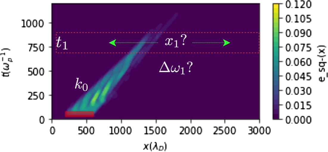
Here, we ask: What happens when a nonlinear electron plasma wavepacket is driven on top of another? To answer this question, we reframe it as an optimization problem and ask: What is the best way to excite a wavepacket that interacts with a pre-existing wavepacket?
We start with a large-amplitude, finite-length electrostatic wavepacket driven by a forcing function with parameters given by

where $x_{i}$ is the location of excitation, $\omega _i$
 is the frequency, $t_i$
 is the time of excitation and $k_i$
 is the wavenumber, of the $i$
 th wavepacket.
Since we seek to excite a second wavepacket that can interact with the detrapped electrons, we stipulate that the phase velocity of the resonant electrons from both wavepackets is roughly the same. For this reason, we set the wavenumber $k_1 = k_0$ . We reparameterize the resonant frequency, $\omega _1$
 , with a frequency shift, $\Delta \omega _1$
 and the linear resonant frequency $\omega _0$
 such that $\omega _1 = \omega _0 + \Delta \omega _1$
 .
.
We use the time of excitation of the second wavepacket, $t_1$ , as an independent variable along with $k_0$
 . For each $t_1$
 and $k_0$
 , we seek to learn functions that produce $x_1$
 and $\Delta \omega _1$
 i.e. we seek to learn $x_1(t_1, k_0, \omega _0)$
 and $\Delta \omega _1( t_1, k_0)$
 . The entire parameter vector for the second wavepacket is given by

This framing is also illustrated in figure 2 where, given $k_0$ and $t_1$
 , we seek functions for $\omega _1$
 and $x_1$
 .
.
Given a first wavepacket with wavenumber $k_0$ and a desired time of second wavepacket excitation $t_1$
 , the task is to learn functions that give the optimal frequency $\omega _1$
 and spatial location $x_1$
 of the second wavepacket.

We reparameterize $\Delta \omega _1$ and $x_1$
 with a neural network with a parameter vector, $\theta ^*$
 , that maximizes the electrostatic energy (minimizes the free energy) and maximizes the difference in the kinetic entropy. These relationships are given by


whereFootnote 2,

and


are the electrostatic energy and difference in the kinetic entropy terms in the loss function, respectively. Also, $f_\text {MX} = f_\text {MX}(n(t, x), T(t, x))$ , $n(t, x) = \int f(t, x, v)\,{\rm d} v$
 , $T = \int f(t, x, v) v^2\,{\rm d} v /n$
 , where $f_\text {MX}$
 is the local Maxwell–Boltzmann distribution. Equation (3.7) describes the deviation of the local distribution function from the equivalent Maxwell–Boltzmann distribution function. It has been used as a measure of the non-Maxwellian-ness by Kaufmann & Paterson (Reference Kaufmann and Paterson2009). The reason we maximize this deviation is because we seek to enhance the likelihood of nonlinear kinetic effects.
We vary the independent variables such that


giving an input space of 35 samples from which we seek to learn these functions.
We are able to reproduce similar model training results using a few different neural network configurations and learning parameters. To summarize that study, we find vanilla multi-layer perceptrons 8 nodes wide and 2 layers deep to be effective, especially when ‘activated’ using the Leaky-Rectified-Linear-Unit function. The specifics behind the neural network, optimizer, and data normalization parameters are provided in the Appendix.
The training simulations are performed with the following parameters. The grid is discretized using $N_x = 6656, N_v = 160, N_t = 1200, t_{\max } = 1100 \omega _p^{-1}, x_{\max } = 6600 \lambda _D$ . Assuming inertial fusion conditions where $n_e = 10^{20}\,\text {cm}^{-3}, T_e = 2$
 keV gives a non-zero collision frequency $\nu _{ee}/\omega _p = 5 \times 10^{-5}$
 (Huba Reference Huba2011) for the simulations shown here. Details on the solvers and forcing function parameters are provided in the Appendix.
Figure 3 shows that the loss value is reduced over the duration of the training process. Each simulation takes approximately 3 minutes to run on a NVIDIA T4 GPU. We train for 60 epochs. The convergence in the loss metric suggests that we were able to train a overparametrized neural network with 35 samples of data in 60 epochs. While Metz et al. (Reference Metz, Freeman, Schoenholz and Kachman2022) discuss that differentiating through the evolution of chaotic dynamical systems can be ill posed, ablation studies indicate that the objective function posed here has a robust minimum. One reason is because the chaotic particle dynamics is subject to dispersion, Landau damping and collisions. This may result in a smoothing of the loss surface. Second, since the objective functions used here are space, time and velocity integrals over the chaotic trajectories, the gradients calculated here may benefit from the smoothness associated with time- and phase-space averaging of a well-behaved ergodic system.

Figure 4 shows the electric field profile for three different simulations. In figure 4(a), only the first wavepacket is excited, and in figure 4(b), only the second wavepacket is excited. In figure 4(c), both wavepackets are excited. Early in time, $t=400 \omega _p^{-1}$ (green), when only the first wavepacket has been excited figures 4(a) and 4(c) agree perfectly. The second wavepacket is excited at $t=500 \omega _p^{-1}$
 . At $t=900 \omega _p^{-1}$
 , once some time has passed after the excitation of the second wavepacket, the first wavepacket has not fully damped away. It is visible as small bumps in figures 4(a) and 4(c). The second wavepacket is also present at this time and easily seen in figure 4(b). A larger-amplitude wavepacket is seen in figure 4(c). Late in time, the difference in amplitude between the second wavepacket in figures 4(b) and 4(c) is obvious. The second wavepacket has nearly damped away in figure 4(b). In figure 4(c), the second wavepacket persists, at nearly the same energy as it was at $t=900 \omega _p^{-1}$
 . We observe this superadditive behaviour, where $f(x) + f(y) \leq f(x+y)$
 , for all wavenumbers we model.
Early in time (green), (c) is the same as (a). Later in time, $t=900 \omega _p^{-1}$ (blue), (a,c) show very similar magnitudes for the first wavepacket near $x=1500 \lambda _D$
 but the second wavepacket excitation is larger in (c) than (b). At $t=1300 \omega _p^{-1}$
 (red), it is clear that (c) is not a superposition of (a,b) because (b) has damped away, while (c) retains electrostatic energy, suggesting the involvement of a superadditive process. (a) First wavepacket only; (b) second wavepacket only; (c) both wavepackets.

To determine the mechanism behind this phenomenon, we turn to the phase-space dynamics. In figure 5, (i) is a space–time plot of the electric field. The two dashed-dot red lines at the front and back of the wavepacket are parallel and indicate the velocity of the wavefront. In figure 5(a)(i), the rear of the wavepacket propagates at a seemingly faster rate than the front. Fahlen et al. (Reference Fahlen, Winjum, Grismayer and Mori2009) describe this as etching of the wavepacket. In figure 5(b), the wave survives for a much longer time, as was also illustrated in figure 4. Figure 5(ii, iii) are phase-space plots with their centre indicated by the intersection of the horizontal timestamp line and the dashed-dot line at the rear wavepacket. The insets (iv) and (v) correspond to the intersection with the dashed-dot line at the front. Insets (ii) and (iv) show the phase space within a window in $\hat {x}$ , while (iii) and (v) are the spatially averaged distribution function. Insets (iii) and (v) serve as a proxy for approximating the propensity of Landau damping in that region. In figure 5(a)(ii, iii), we see that the rear of the wavepacket is Maxwellian. Fahlen et al. (Reference Fahlen, Winjum, Grismayer and Mori2009) showed this is why the rear of the wavepacket damps faster than the front, as in figure 5(a)(i).
Left – space–time plot of the electrostatic energy shows the long-lived wavepacket in (b) where the field in (b) survives for a longer duration than in (a). The horizontal line indicates the timestamp of the snapshots in the middle and right. The diagonal dashed-dot lines indicate the spatial location of the snapshots in the middle and right. Middle phase-space plots at the back (top) and front (bottom) of the wavepacket. In (b), the phase space shows significant activity at the back of the wavepacket while in (a), the distribution function is nearly undisturbed. Right – T = the spatially averaged distribution function. This confirms the fact that the distribution function has returned to a Maxwell–Boltzmann at the back of the wavepacket in (a), while in (b), the distribution function remains flat at the phase velocity of the wave. This is the reason behind the loss of damping. (a) Second wavepacket only; (b) both wavepackets.

In the simulations described here, the plots in figure 5(b) show that the distribution function at the back of the wavepacket has trapped particle activity (figure 5(b)(ii)) and there is a near zero slope at the phase velocity of the wave (figure 5(b)(iii)). Both plots show that the slope is negligible because of the arrival of streaming detrapped particles from the first wavepacket. Due to this effect, the re-emergence of Landau damping that occurs due to the loss of trapped particles in isolated wavepackets no longer occurs here. This results in a reduction of the etching and the wavepacket propagates freely for some time while the particles from the first wavepacket propagate and arrive at the rear of the second wavepacket.
Figure 6 shows the results of the optimization process for the resonant spatial location. For $t_1 < 500 \omega _p^{-1}$ , the resonant location decreases as a function of wavenumber. From analysing phase space, we have determined that the spatial location is related to the resonant electron transport i.e. $x_1 \approx v_{ph} t_1$
 . Waves with larger wavenumbers have smaller phase velocities. Because of this, the resonant spatial location decreases as a function of wavenumber. For a fixed wavenumber, figure 6(b) shows a locus of points in space–time where long-lived wavepackets can be excited in the presence of a pre-existing wavepacket. This suggests the possibility of a critical space–time radius within which collisional relaxation has yet to occur, and nonlinear effects can be exploited.
(a) Learned function for the resonant spatial location as a function of wavenumber of the first wavepacket and time of excitation of the second. (b) The locus in space–time (in red) where long-lived wavepackets can be excited for $k=0.28$ : (a) $x_1(k_0, t_1)$
 ; (b) space–timelocus.

Likewise, we also learn the dependence of the optimum frequency shift as a function of $k_0$ and $t_c$
 , as shown in figure 7. The learned frequency shift, a few per cent here, is similar in magnitude as to that observed in previous work related to SRS (Ellis et al. Reference Ellis, Strozzi, Winjum, Tsung, Grismayer, Mori, Fahlen and Williams2012). Furthermore, the frequency shift increases in magnitude as a function of wavenumber. As before, waves with larger wavenumbers have smaller phase velocities, and therefore, interact with more particles. Because of this, waves with larger wavenumbers have a larger nonlinear frequency shift associated with them, as we see here (Manheimer & Flynn Reference Manheimer and Flynn1971; Dewar Reference Dewar1972; Morales & O'Neil Reference Morales and O'Neil1972; Berger et al. Reference Berger, Brunner, Chapman, Divol, Still and Valeo2013).
The learned function for the frequency shift $\Delta \omega _1(k_0, t_1)$ as a function of wavenumber of the first wavepacket, $k_0$
 , and time of excitation, $t_1$
 , of the second.

4. Conclusion
We show how one may be able to discover novel physics using differentiable simulations by posing a physical question as an optimization problem. This required domain expertise in determining which functional dependencies to learn using neural networks.
In figure 1, we show how one may adapt an existing computational science workflow to the autodidactic process described here. In the work performed here, this process enabled the discovery of functional relationships between optimal parameters in a four-dimensional search space with known bounds but an unknown resolution requirement. We trained the model over a coarse grid in $k_0$ and $t_1$
 , and learned functions for $x_1$
 and $\omega _1$
 . Using gradient descent here allows an escape from the curse of dimensionality and reduces the problem from a four-dimensional search to a two-dimensional search $+$
 two-dimensional gradient descent.
This discovery process is not limited to differentiable simulations. While in figure 1, $\mathcal {V}$ represents a PDE solve, it only needs to be a AD-enabled function that is a model for a physical system. For example, rather than a PDE solve, $\mathcal {V}$
 could represent a pre-trained neural-network-based emulator for experimental data. In such a scenario, one may be able to learn forcing function parameters for an experiment using the proposed workflow.
In the neural network literature, the gradient required for the update is $\partial \mathcal {S} / \partial \theta = \partial \mathcal {S} / \partial \mathcal {G} \times \partial \mathcal {G} / \partial \theta$ . We see that this is the same as (2.5) after the addition of one more node in the computational graph for $\mathcal {V}$
 , the function that models the physical system. This allows the neural network training process to become unsupervised and data efficient.
It remains to be determined how the physical mechanism discussed here behaves over a range of amplitudes and collision frequencies in addition to the wavenumber scan we perform here. Reduced models of the wavepacket dynamics in SRS remain useful for the development of inertial confinement fusion schemes where laser–plasma instabilities occur.
Differentiating through an entire simulation, in this case, required the intermediate storage of all $N_t \times N_x \times N_v$ arrays representing the distribution function in time and phase space. To enable this on a single NVIDIA T4 GPU, we use gradient checkpointing (Griewank & Walther Reference Griewank and Walther2000; Chen et al. Reference Chen, Xu, Zhang and Guestrin2016), as implemented in JAX, at every timestep. That is, we require that the Jacobian of the function representing a single timestep recompute its internal linearization points rather than save them to memory during the forward pass. Another technique by which we can save on the memory cost is by improving the efficiency of the accumulation of the Jacobian e.g. as proposed in Naumann (Reference Naumann2004) and similar works. An example application towards a PDE is provided by Oktay et al. (Reference Oktay, McGreivy, Aduol, Beatson and Adams2021). A final route to memory savings we wish to highlight here is by solving a backwards-in-time ordinary-differential equation for the adjoint (Pontryagin Reference Pontryagin1987; Chen et al. Reference Chen, Rubanova, Bettencourt, Duvenaud, Bengio, Wallach, Larochelle, Grauman, Cesa-Bianchi and Garnett2018). For modelling systems of higher-dimensionality, larger time scales and other constraints that require larger in-memory calculations, it will be crucial to leverage methods that help circumvent the memory burden encountered with differentiable simulations.
Acknowledgements
A.J. wishes to acknowledge D. Strozzi for early and continued encouragement, S. Hoyer for introducing him to JAX, M. Poli and S. Masseroli for the perspectives of ML researchers and B.B. Afeyan, W.B. Mori and B.J. Winjum for discussions on nonlinear electron plasma waves. A.J. also gratefully acknowledges travel support from Syntensor Inc. The authors thank the anonymous reviewers for valuable feedback.
Editor William Dorland thanks the referees for their advice in evaluating this article.
Declaration of interests
The authors report no conflict of interest.
Appendix A. Simulation details
We reproduce the solvers in Joglekar & Levy (Reference Joglekar and Levy2020) using JAX (Bradbury et al. Reference Bradbury, Frostig, Hawkins, Johnson, Leary, Maclaurin, Necula, Paszke, VanderPlas and Wanderman-Milne2018) and Haiku (Hennigan et al. Reference Hennigan, Cai, Norman and Babuschkin2020) to allow the usage of AD, judicious placement of neural networks as well as the ability to run on GPU.
A.1. Solvers
A.1.1. Vlasov equation
We discretize $f(t,x,v)$ with $f^n(x_i,v_j)$
 . To calculate $f^{n+1}$
 , we use the sixth-order Hamiltonian integrator introduced in Casas et al. (Reference Casas, Crouseilles, Faou and Mehrenberger2017).
As in Joglekar & Levy (Reference Joglekar and Levy2020) and Thomas (Reference Thomas2016), the individual components of the left-hand side of (1.1) are solved using operator splitting, spectral discretizations and exponential integration as given by


where $\mathcal {F}_{\{x,v\}}$ are the Fourier transforms in space and time, respectively. We use a spectral solver for Gauss's law such that

A.1.2. Fokker–Planck Equation
Two simplified versions of the full Fokker–Planck operator are implemented. The first of these implementations is given in Lenard & Bernstein (Reference Lenard and Bernstein1958) and has the governing equation given by

where

is the thermal velocity of the distribution. We term this the LB operator as per the authors' names. The second of these implementations is given in Dougherty (Reference Dougherty1964) and has a governing equation given by

where

is the mean velocity of the distribution and

is the thermal velocity of the distribution while accounting for the mean velocity. We term this the DG operator as per the author's name. The DG operator extends the LB operator by enabling momentum conservation for distribution functions that have a non-zero mean velocity.
We discretize these equations using a backward Euler method with centre differencing space. This procedure results in the timestep scheme given by

where


where $\bar {v} = v$ or $\bar {v} = v - \underline {v}$
 depending on the implementation. This forms a tridiagonal system of equations that can be directly inverted.
A.2. Parameterizing the Ponderomotive Driver
Similar to that presented by Afeyan et al. (Reference Afeyan, Casas, Crouseilles, Dodhy, Faou, Mehrenberger and Sonnendrücker2014), the ponderomotive driver is parametrized using space–time envelopes created using hyperbolic tangents given by

where $\boldsymbol {s}$ can be $\boldsymbol {x}$
 or $\boldsymbol {t}$
 , $p_{R/L} = p_c \pm p_w/2$
 , and the rest of the parameters are given by the set $p_i = (p_{c}, p_{w}, p_{r}, k, a,\omega, \Delta \omega )$
 . Using (A13), the overall profile in space and time is given by

In the simulations performed in this work, we specify the following.
(i) For each individual set of driver parameters, $p_{r, \boldsymbol {x}} / \lambda _D = p_{r, \boldsymbol {t}} / \omega _p^{-1} = p_r = 10$
 , $p_{w, \boldsymbol {x}} = 400 \lambda _D$ and $p_{w, \boldsymbol {t}} = 50 \omega _p^{-1}$.
(ii) For the first driver, $p_{c, \boldsymbol {t}} = 50 \omega _p^{-1}$
, $p_{c, \boldsymbol {x}} = 400 \lambda _D$.


This leaves $p_c$ for the second driver and the wave parameters, $k, a, \omega, \Delta \omega$
 to be varied in this work. For readability, in the manuscript body, we use $p_{i, c, \boldsymbol {x}} = x_i$
 and $p_{i, c, \boldsymbol {t}} = t_i$
 .
.
A.3. Physical domain
We initialize the plasma distribution function with a Maxwell–Boltzmann distribution with $n_0 = 1.0, v_{{\rm th}0} = 1.0$ , $f(t=0, x, v)= \exp (-v^2) / \sqrt {{\rm \pi} }$
 .
.
In order to ensure that there is no unwanted interference from particles transiting across the periodic boundary, thermal boundaries are implemented using a Krook-type collision operator (Bhatnagar, Gross & Krook Reference Bhatnagar, Gross and Krook1954). The equation is solved directly and exactly, and the solution at the new timestep is given by

where $f_\text {MX}(n_0, v_{{\rm th}0}) = n_0 \exp (-v^2/v_{{\rm th}}^2) / \sqrt {{\rm \pi} v_{{\rm th}}^2}$ .
.
By having non-zero $\nu _K$ only in a small localized region at the boundary, as also described by Strozzi et al. (Reference Strozzi, Williams, Langdon and Bers2007), and as shown in figure 8, the particles are absorbed in a fixed Maxwellian, similar to having a thermal boundary condition. This localization is also performed using the hyperbolic tangent parameterization from (A13) but using $1 - g(p, \boldsymbol {x})$
 . In this case, $p_c = 3300, p_w = 6500, p_r = 10$
 .
.
We implement thermal-bath boundaries for the plasma by artificially increasing the collision frequency of the Krook operator at the edges using (A13) and $p_L = 500, p_R = 6000, p_{wL} = p_{wR} = 500$ . (a) Entire box; (b) zoom in.

Appendix B. Neural network and optimizer details
We implement our solver framework using Haiku (Hennigan et al. Reference Hennigan, Cai, Norman and Babuschkin2020). In this work, we leverage a vanilla multi-layer perceptron constructed using linear (fully connected) layers and nonlinear (activation) functions. We train this model with the following architectures:


where $\mathcal {L}(N)$ is the linear layer with $N$
 nodes,


and $\mathcal {T}(x) = \tanh (x)$ . Also, $\mathcal {I}$
 and $\mathcal {O}$
 are the arrays representing the inputs to and outputs from the neural network. We observe that the higher capacity architectures we tested converge faster as does training with the Leaky-ReLU function. We use the ADAM optimizer (Kingma & Ba Reference Kingma and Ba2017) implemented via Optax (Babuschkin et al. Reference Babuschkin, Baumli, Bell, Bhupatiraju, Bruce and Buchlovsky2020). We train the model using learning rates of $0.05, 0.01, 0.005$
 and we find that the smallest learning rate performs the best. We do not perform extensive architecture and hyperparameter searches because the primary goal here is to discuss and apply the capability of function approximation towards physics discovery, rather than learning the best possible approximation.
Appendix C. Data normalization
Much like how simulations are generally conducted in normalized units, neural networks are typically trained on normalized data. We need to do the same here so we normalize the inputs between 0 and 1. As specified in the body of the text, our inputs to and outputs from the neural network are given by


We augment the input vector with $\omega _0, k_1, \omega _1$ and normalize the inputs to and outputs of the neural network such that


It is important to note that, since $k_0 = k_1, \omega _1 = \omega _0$ and that $\omega = \omega (k)$
 through the electrostatic dispersion relation, there is no new information being added to the training process by this augmentation. However, we do provide the training process with a sophisticated reinterpretation of the existing information by providing $\omega = \omega (k)$
 .
.
We normalize the 5 input parameters to scale between 0 and 1 such that $0.26 < k < 0.34, 1.05 < \omega < 1.3$ and $400 < t_1 < 800$
 i.e. $\tilde {k} = (k - k_{\min }) / (k_{\max } - k_{\min })$
 and so on.
The output parameters, $\tilde {x}_1, \widetilde {\Delta \omega _1}$ , are renormalized slightly differently because the outputs range from -1 to 1. For $x_1$
 , we allow the entire domain except for regions near the boundaries. We choose the bounds of the frequency shift by measuring typical nonlinear frequency shifts observed for idealized, periodic nonlinear electron plasma waves. We normalize each such that $500 < x_1 < 6000$
 and $-0.06 < \Delta \omega _1 < 0.06$
 . This gives $x_n = 2750, x_s = 3250$
 and $\omega _n = 0.06, \omega _s = 0$
 .
.
Appendix D. Validation tests
We reproduce the tests implemented and shown in Joglekar & Levy (Reference Joglekar and Levy2020).
(i) Gauss's law.
(ii) Landau damping.
(iii) Density conservation of both implementations of the Fokker–Planck operators.
(iv) Momentum conservation of the DG implementation of the Fokker–Planck implementation.
(v) Energy conservation of the LB and DG implementations of the Fokker–Planck operator.
D.1. Validating the differentiable simulator by recovering known physics
We describe an additional test here which involves recovering the linear, small-amplitude Langmuir, or electrostatic, resonance using a gradient-based method enabled by this AD-capable implementation. This ensures that the gradients given by the AD system are representative of physical phenomenon.
D.1.1. Electrostatic waves
A fundamental wave in plasma physics is the electrostatic wave in unmagnetized plasmas. The dispersion relation is given in numerous textbooks, and reproduced here as

where $\omega _e$ is the plasma frequency, $k$
 is the wavenumber, $\omega$
 is the resonant frequency and $v$
 is the independent variable representing the velocity in the integral. Also, $g(v)$
 is the normalized distribution function of the plasma particles. This equation has been solved numerically and a lookup table for $\omega$
 as a function of $k$
 is provided in Canosa (Reference Canosa1973).
We test the capability of our differentiable simulator framework by reproducing those calculations. To do so, we implement the functionality in figure 1(c). We choose a loss function that minimizes free energy given by

In this test, we launch plasma waves using a ponderomotive driver in a box with periodic boundary conditions. For each optimization, the wavenumber $k$ and the box size $x_{\max }$
 change. We provide a lower bound of $0.5$
 and an upper bound of $1.4$
 to the optimization algorithm. We use the L-BFGS algorithm implemented in SciPy (SciPy 1.0 Contributors et al. Reference Virtanen, Gommers, Oliphant, Haberland, Reddy, Cournapeau, Burovski, Peterson and Weckesser2020). We set $f_\text {tol}=r_\text {tol}=10^{-12}$
 . The remaining parameter is the frequency $\omega$
 that will minimize the value given by (D2) and ensure that it is within 2 decimal places of the direct solution to (D1), which is calculated using the root finder in SciPy.
We optimize for the resonant frequency for 100 random wavenumbers using gradients acquired using AD and finite difference (FD) and plot the performance. Figure 9 shows the distributions of the number of iterations required for each gradient-calculation method. We see that the finite-difference method requires significantly more evaluations where the maximum number of evaluations is larger by a factor of 2. One of the optimization runs requires 80 evaluations with FD, and 40 with AD. Similarly the mean and median values are smaller by a factor of 2 for AD in comparison with those for FD. It is important to note that these results are for single-variable searches. When the dimensionality of the search space increases, using FD becomes impractical. When using neural networks that are parametrized by $\gg \mathcal {O}(10)$ parameters, using FD is simply not possible, and one must use AD to acquire gradients.
We run 100 optimizations over random wavenumbers in order to quantify the performance of gradients acquired using finite difference (FD) and AD. The plot shows a comparison of the number of iterations needed to converge to a local optimum.


 Open access