

Introduction
Recent studies have shown that mass loss from the Antarctic ice sheet is strongly linked to changes in its floating ice shelves, which have a buttressing influence on its outlet glaciers and ice streams (Reference De Angelis and SkvarcaDe Angelis and Skvarca, 2003; Reference Rignot, Casassa, Gogineni, Krabill, Rivera and ThomasRignot and others, 2004; Reference Scambos, Bohlander, Shuman and SkvarcaScambos and others, 2004). It is therefore vital that we improve our ability to (1) accurately represent ice shelves in coupled Earth system models that are used to predict changes in the mass balance of the ice sheet and consequent global sea-level changes, and (2) produce baseline maps of the current configuration of ice shelves against which future change can be measured. Both these activities require knowledge of the basic geometry of ice shelves including ice-shelf elevation and thickness (e.g. Reference VaughanVaughan and others, 2006; Reference Bamber, Gomez-Dans and GriggsBamber and others, 2009), water column thickness (e.g. Reference Galton-Fenzi, Maraldi, Coleman and HunterGalton-Fenzi and others, 2008) and the location of the perimeter of the floating ice (e.g. Reference Fricker, Coleman, Padman, Scambos, Bohlander and BruntFricker and others, 2009). Mapping of each of these parameters is subject to large uncertainty.
In this paper, our primary goal is to develop an improved map of the location and extent of the grounding zone (GZ) of the Ross Ice Shelf (RIS), Antarctica. The GZ is the region of the ice sheet where conditions vary from grounded ice sheet to freely floating ice shelf, typically over a distance of a few km, across the grounding line (GL). The new GZ map provides input for ice-sheet models, serves as a baseline map against which future changes can be assessed and contributes to other glaciological and oceanographic investigations. Our approach uses repeat-track analysis of laser altimeter data from the Ice, Cloud, and land Elevation Satellite (ICESat) following the methodology described elsewhere (Reference Fricker and PadmanFricker and Padman, 2006; Reference Fricker, Coleman, Padman, Scambos, Bohlander and BruntFricker and others, 2009). We use the results to assess the strengths and limitations of previously published GL maps for the RIS (Reference GrayGray and others, 2002; Reference Horgan and AnandakrishnanHorgan and Anandakrishnan, 2006; Reference Scambos, Haran, Fahnestock, Painter and BohlanderScambos and others, 2007). Our study demonstrates the advantage of multi-sensor analyses for developing an accurate benchmark GZ map and improving our understanding of the variable structure of the GZ around the RIS.
Mapping the Grounding Zone
The typical geometry of the GZ is shown schematically in Figure 1. Several distinct features are associated with the GZ. The true GL (point G) is the point separating grounded ice from floating ice. Most glaciological and oceanographic applications require knowledge of the location of point G; however, this is a subglacial feature that can only be precisely located through surface surveys employing geophysical methods (e.g. radio-echo sounding and active seismic sounding). Mapping the GL over a large area in this way is impractical. Thus, GL maps are generally compiled by estimating the location of one or more of the four surface features of the GZ that are detectable in satellite data (i.e. points F, H, Im and Ib in Fig. 1).
Schematic diagram showing the key features of a typical ice-shelf GZ, based on Reference SmithSmith (1991), Reference VaughanVaughan (1994) and Reference Fricker, Coleman, Padman, Scambos, Bohlander and BruntFricker and others (2009). Point F is the landward limit of ice flexure from tidal movement; point G is the true GL where the grounded ice first loses contact with the bed; point I b is the break-in-slope; point Im is the local minimum in topography; and point H is the hydrostatic point where the ice first reaches approximate hydrostatic equilibrium.
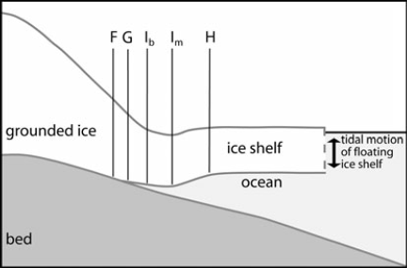
Point F is the landward limit of ice flexure, and point H is the ‘hydrostatic point’ where the ice shelf first settles to near equilibrium with the ocean. Between these points, ice undergoes flexure induced by short-term sea-level variations within the sub-ice-shelf cavity. The principal causes of these variations are ocean tides and the inverse barometer effect (IBE), the latter being the ocean response to change in atmospheric pressure, Pair. Tidal range around Antarctica is typically 1–2 m but is higher locally, up to ∼ 8 m in the southwestern corner of the Filchner-Ronne Ice Shelf (Reference Padman, Fricker, Coleman, Howard and ErofeevaPadman and others, 2002). The IBE response is ∼–0.01 m per +1 hPa change in P air, giving a typical range of order 0.1 m, but up to ∼0.5 m under exceptional atmospheric conditions (Reference Padman, Erofeeva and JoughinPadman and others, 2003). Landward of point F, no ocean-induced vertical motion of the ice surface occurs; seaward of point H, the ice is close to being in hydrostatic equilibrium with the ocean. The distance between points F and H is an approximation for the GZ width which is typically several km, and varies according to local ice thickness and properties, and local bed topography and properties.
There is often a topographic minimum (point Im) associated with a non-hydrostatic ice flexure response just seaward of point F (Reference VaughanVaughan, 1994) and a break-in-slope (point Ib). In some regions, there can be multiple breaks-in-slope near the grounding line, as observed in satellite altimeter profiles across the GZ (e.g. on the Amery Ice Shelf; see Reference Fricker, Coleman, Padman, Scambos, Bohlander and BruntFricker and others, 2009, fig. 6).
As described by Reference Fricker, Coleman, Padman, Scambos, Bohlander and BruntFricker and others (2009; see their table 1), different satellite sensors can be used to find different combinations of the surface GZ features (F, H, Im and Ib), through a variety of analyses, which can be divided into two categories: dynamic and static.
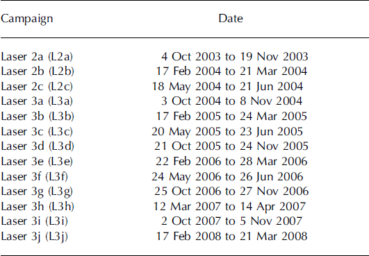
Acquisition dates for the 13 ICESat campaigns acquired from October 2003 to March 2008
Dynamic methods take advantage of ocean-induced temporal changes in the ice surface elevation between points F and H. Synthetic aperture radar (SAR) interferometry (InSAR; Reference Goldstein, Engelhardt, Kamb and FrolichGoldstein and others, 1993) is a dynamic method that can provide a continuous, high-resolution two-dimensional map of points F and H. ICESat repeat-track analysis is another dynamic method, and can estimate the location of all surface features along discrete track segments across the GZ.
Static methods are based on a single gridded field, either a satellite image product or a digital elevation model (DEM). In visible image products, including the Moderate Resolution Imaging Spectroradiometer (MODIS) Mosaic of Antarctica (MOA; Reference Scambos, Haran, Fahnestock, Painter and BohlanderScambos and others, 2007) and Landsat Image Mosaic of Antarctica (LIMA; Reference BindschadlerBindschadler and others, 2008), small-scale surface topographic features associated with the onset of flotation are visible through gradients in surface shading. These features include flow-stripe disruption, surface manifestations of basal crevasses, and a break in the surface slope. Reference Scambos, Haran, Fahnestock, Painter and BohlanderScambos and others (2007) estimated the location of the GL from the MOA as the most seaward continuous break-in-slope that is landward of other indicators of the GL. Reference Horgan and AnandakrishnanHorgan and Anandakrishnan (2006) estimated the location of the GL based on a surface-slope analysis of a high-resolution DEM derived from ICESat elevation data. They observed a ‘ramp’ of relatively high surface slope that was collocated with the GZ determined from in situ methods including GPS and observations of bottom crevassing in radar transects. They calculated the first spatial derivative to determine the extent of this ramp, then took the centre of this ramp as their estimate of GL location.
The challenge we face is inferring the true GL (point G) from the different surface features identified by the various satellite techniques. For dynamic methods, a good proxy for the GL is point F, which is usually the nearest detectable surface feature to point G. Point F is slightly landward of point G (Fig. 1). For static methods, we are restricted to inferring the GL from dynamically based expectations of ice surface slope changes at the GL, where the basal stress conditions change from those imposed by bed (rock or till) to those imposed by water. In some places, however, the ice surface response associated with the GL is quite subtle, and the most prominent change in surface topography is observed several km landward of point F. This observation has been used to locate ‘ice plains’, defined as regions with low surface slopes that are only ‘lightly grounded’. Thus, ice plains are identified as areas where the hydrostatic height anomaly, i.e. the difference between the measured surface elevation and the surface elevation calculated assuming buoyancy and the measured ice thickness, is small, on the order of tens of meters. Such an analysis, based on airborne radio-echo sounding data, allowed Reference Corr, Doake, Jenkins and VaughanCorr and others (2001) to identify an ice plain on Pine Island Glacier and to define a ‘coupling point’ between the lightly grounded ice plain and the fully grounded ice sheet. The surface expression of this coupling point was associated with the dominant break-in-slope in this region. Similarly, Reference Fricker and PadmanFricker and Padman (2006) identified an ice plain in the southern Filchner–Ronne Ice Shelf (first suggested by Reference Jankowski and DrewryJankowski and Drewry (1981) from geophysical data) based on a large separation between their estimations of points F and Ib derived from ICESat repeat-track analysis.
We propose that the most robust proxy for the location of the GL is point F estimated from dynamic methods when appropriate data are available. The locus of point F can be accurately estimated from SAR images if sufficient images acquired at suitable times in the tidal cycle exist to create a ‘differential’ SAR interferogram (DSI; Reference RignotRignot, 1998b; Reference Fricker, Coleman, Padman, Scambos, Bohlander and BruntFricker and others, 2009). This process allows for removal of the effects of mean lateral flow of ice across the GZ by assuming that it is the same in each interferogram. InSAR-based techniques are limited primarily by SAR data availability; InSAR data from the European Remote-sensing Satellite (ERS) tandem mission can also lead to inadequate sampling of tidal variability (Reference Fricker, Coleman, Padman, Scambos, Bohlander and BruntFricker and others, 2009). ICESat repeat-track analysis also provides accurate mapping of point F; however, ICESat can only provide estimates at discrete locations where tracks cross the GL (track spacing depends on latitude but is of order 10 km over most Antarctic ice shelves).
When the location of point F is not available from dynamic methods, point Ib estimated by static methods frequently provides a reasonable, continuous approximation for the GL. However, as we have noted above, there can be more than one break-in-slope in the vicinity of the GL, and the one closest to the GL may not be the most prominent.
While our primary goal is the best possible estimate of the location of the GL, knowledge of other GZ features is also valuable for several applications. For example, mass flux calculations for ice shelves (e.g. Reference RignotRignot and others, 2008) require knowledge of point H since this is the most upstream point where the ice thickness can be derived from the surface elevation and an ice density model through the hydrostatic assumption. Additionally, the locations of point Ib, where they deviate significantly from point F, provide insight into the structure of the GZ that can contribute to our understanding of ice-sheet dynamics. Thus, our goal is to map all major surface GZ features.
Methods: Mapping the Grounding Zone with ICESat
The primary instrument carried by ICESat (Reference Schutz, Zwally, Shuman, Hancock and DiMarzioSchutz and others, 2005) is the Geoscience Laser Altimeter System (GLAS). This altimeter samples 50–70 m diameter footprints every ∼172 m along each track, with elevation retrieval precision and accuracy of ∼2 and ∼14cm, respectively (Reference ShumanShuman and others, 2006). Since October 2003, ICESat has operated in ‘campaign’ mode, with discrete 33 day data acquisition periods capturing the same 33 day sub-repeat cycle of a 91 day exact repeat cycle. Data acquisition occurs two or three times per year (Table 1; for more details of this operation mode see Reference Schutz, Zwally, Shuman, Hancock and DiMarzioSchutz and others, 2005; Reference Fricker, Coleman, Padman, Scambos, Bohlander and BruntFricker and others, 2009).
The latitudinal limit of ICESat (86°S) provides coverage over all of Antarctica’s ice shelves. The track spacing is ∼5 km at 85° S in the southernmost part of the RIS and ∼20 km at 78° S near the RIS ice front. ICESat ground tracks do not repeat exactly: ICESat points towards a reference ground track, but the post-processed footprints can be offset from this by up to 200 m.
Our approach to estimating points Ib, F and H using ICESat repeat-track altimetry closely follows the technique described elsewhere (Reference Fricker and PadmanFricker and Padman, 2006) and used by Reference Fricker, Coleman, Padman, Scambos, Bohlander and BruntFricker and others (2009) for mapping the Amery Ice Shelf GZ. Here we summarize only the key features of the approach.
We used the ICESat product GLA12 (GLAS Antarctic and Greenland Ice Sheet Altimetry Data product), release 428, for 13 ICESat campaigns acquired between October 2003 and March 2008 (Table 1). We obtained the following parameters from the GLA12 records: geolocated GLAS footprint location; ocean tide and ocean-tide loading corrections; saturation correction; instrument gain; and received energy (Reference Schutz, Zwally, Shuman, Hancock and DiMarzioSchutz and others, 2005; Reference ShumanShuman and others, 2006). The GLAS footprint locations (latitude, longitude and elevation) are provided on the TOPEX/Poseidon ellipsoid, which we converted to WGS-84 for consistency with other polar altimetry datasets. We applied the saturation correction to the elevations.
The ICESat elevations provided in the GLA12 release 428 have had predicted ocean and load tides removed using the GOT99.2 global ocean-tide model. Since the techniques we employed in finding the GZ are dependent on detecting the tidal signal on the ice shelf, we ‘re-tided’ these elevations, i.e. removed the applied tidal correction from the GLA12 elevations. We then analyzed the re-tided data on a track-by-track basis, following the procedures described elsewhere (Reference Fricker and PadmanFricker and Padman, 2006; Reference Fricker, Coleman, Padman, Scambos, Bohlander and BruntFricker and others, 2009). We first removed cloud-affected repeated passes (based on gain and energy values) and repeated passes with large cross-track offsets (greater than ∼100m). For this study, we did not correct along-track elevations for cross-track slopes as reported by Reference Smith, Fricker, Joughin and TulaczykSmith and others (2009) in their studies of temporal changes on grounded ice, since the assumption of time-independent cross-track slope is not valid in the GZ.
To allow calculation of temporal changes in elevation, we resampled the along-track data by interpolation to a nominal reference track whose location was the average of all of the repeated passes. We used a coordinate system defined with respect to this reference track; this is better than resampling in latitude as first used by Reference Fricker and PadmanFricker and Padman (2006), as that method introduced additional biases. We used an along-track interpolation interval of 200 m.
After resampling the data, we calculated a reference elevation profile from the mean elevation of the cloud-free repeated passes in the vicinity of the GL estimated from the MOA (Reference Scambos, Haran, Fahnestock, Painter and BohlanderScambos and others, 2007). We then calculated a set of ‘elevation anomalies’, obtained by subtracting the reference elevation profile from the elevation profiles of each individual repeated pass. For each track, we visually estimated points Ib, F and H. Point Ib was estimated from the set of elevation profiles (Fig. 2a). As mentioned above, there is often more than one break-in-slope near the GL, including those farther upstream associated with the coupling lines of ice plains. Generally, the MOA-based estimate of GL location is close to a break-in-slope in the ICESat elevation profiles. Thus, with few exceptions, we selected the most prominent break-in-slope in close proximity (∼2 km) to the MOA GL as point Ib.
Example of the estimation of GZ parameters (points Ib, F and H) from ICESat repeat-track analysis applied to track 177, which crosses the RIS GZ approximately normal to the MOA GL (location shown in Fig. 3). (a) Set of ‘re-tided’ ICESat surface elevation profiles for all valid repeated passes of track 177. We estimate the location of point I b from the set of elevation profiles and compare it with the GL location estimated from the MOA. (b) Set of elevation anomalies, calculated by subtracting the reference elevation profile (i.e. the mean of all elevation profiles) from the individual elevation profiles. At the right are the tide height predictions from the CATS 2008a tide model (also referenced to zero mean) that correspond to each repeated pass. We estimate the location of points F and H from the set of elevation anomalies, using the tidal predictions as a guide.

For most tracks, there were sufficient cloud-free tracks across the GZ with adequate temporal sampling of tide height, so we were able to estimate the locations of points F and H from the elevation anomaly plots (Fig. 2b). This was facilitated using tide height predictions from the Circum-Antarctic Tidal Simulation model version 2008a (‘CATS 2008a’), a high-resolution (δx=4km) update of previous Antarctic regional models described by Reference Padman, Fricker, Coleman, Howard and ErofeevaPadman and others (2002). We calculated the approximate tidal contribution for each repeated pass, seaward of the GZ, using the tide model ocean grid node closest to ICESat point Ib. We interpret the region where the elevation anomaly is close to zero (the region to the left of point F in Fig. 2b) as fully grounded ice, and the region where the elevation anomaly is consistent with the tidal predictions (to the right of point H in Fig. 2b) as fully floating (hydrostatic) ice shelf. The tide height predictions provide an independent check that elevation anomalies are due to tide-induced ice flexure rather than other factors. The region between points F and H is the zone of ice flexure, which closely approximates the GZ; both points can migrate with the tide (Reference Fricker and PadmanFricker and Padman, 2006). When possible, we estimated point F using the repeated passes sampled at the tidal extremes, which biases point F slightly toward the land compared to its location at mean sea level (zero tides). We estimated point H where the gradient of each elevation anomaly curve first tends to zero and is consistent with the tidal height predictions.
Results and Discussion
Using the repeat-track technique, we analyzed 403 ICESat tracks that crossed the RIS GL (including the RIS perimeter, islands and ice rises) to estimate the location of points F, H and Ib. Due to multiple GL crossings by some tracks, this resulted in estimation of 491 sets of GZ points (Fig. 3). The resultant map allows us to assess the structure of the GZ and the quality of previous GL maps. Below, we summarize the variation in GZ width, and show several examples that demonstrate both the power of this technique and the limitations of this and other GL mapping methods.
Estimated locations of ICESat-derived GZ surface features (point F, yellow, and point H, cyan) around the perimeter of the RIS, including its islands and ice rises. ICESat ground tracks for laser 2a are shown as black lines. The blue line is point I b estimated by MOA (Reference Scambos, Haran, Fahnestock, Painter and BohlanderScambos and others, 2007). ICESat tracks used in Figures 2, 4 and 5 are indicated as white lines and are numbered. Background image is MODIS MOA image from the US National Snow and Ice Data Center (NSIDC; Reference Scambos, Haran, Fahnestock, Painter and BohlanderScambos and others, 2007).

ICESat-derived GZ width
The local GZ width is approximated by separation between points F and H, normal to the GL. However, ICESat tracks intersect the GZ at a range of angles from perpendicular to almost parallel; therefore, the along-track distance between points F and H is generally an overestimate of the width of the GZ. To correct for this effect, we assume that the continuous GL estimate from the MOA provides a reasonable estimate of the local orientation of the GL determined at the discrete location of each ICESat track. With this assumption, we obtained a width of the GZ at each location. The mean width is ∼3.2 km, and the standard deviation is 2.6 km. In two cases, the GZ width exceeds 10 km.
Comparison of ICESat-derived points with other GL maps
We compared the results of our ICESat analyses with previously published GL maps: (1) point F from single-difference InSAR derived by Reference GrayGray and others (2002), who reported a history of GL estimates for the Siple Coast and updated the map with their own interpretation (hereafter denoted ‘Gray2002’); (2) point Ib for the entire Antarctic based on the MOA (Reference Scambos, Haran, Fahnestock, Painter and BohlanderScambos and others, 2007); and (3) the GL for the Siple Coast based on a surface-slope analysis of a DEM derived from ICESat altimetry by Reference Horgan and AnandakrishnanHorgan and Anandakrishnan (2006), hereafter denoted ‘H&A2006’.
We find that, in general, point F estimated from ICESat repeat-track analysis technique is within ∼ 2 km of the MOA and Gray2002 GLs and is usually close (∼5 km) to the H&A2006 GL. However, there are numerous areas around the GL where our ICESat GZ features deviate significantly from these maps, including the outflow region of Reedy and Leverett Glaciers, and near Engelhardt Ice Ridge just east of Crary Ice Rise (Fig. 3).
In the vicinity of the outflow of Reedy and Leverett Glaciers, south of Mercer Ice Stream along the base of the Transantarctic Mountains, the ICESat GL (point F) generally agrees well with the DEM-based H&A2006 GL and the InSAR-based Gray2002 point F (Fig. 4). However, the offset between the MOA-derived GL and these other maps can exceed 60 km in places. We hypothesize that the MOA technique fails in the vicinity of the outflow of Reedy and Leverett Glaciers because the surface expression of the transition from grounded to floating ice across the GL becomes more subtle as the relative thickness of the ice increases in this region.
The southern limit of the RIS in the outflow of Reedy and Leverett Glaciers. Yellow and cyan points are ICESat-derived estimates of points F and H, respectively; blue line is point I b estimated by MOA (Reference Scambos, Haran, Fahnestock, Painter and BohlanderScambos and others, 2007); white line is the GL location estimated by H&A2006; and red lines are point F estimated by Gray2002 (dotted in regions of lower confidence). Background is MODIS MOA image from NSIDC (Reference Scambos, Haran, Fahnestock, Painter and BohlanderScambos and others, 2007).

Farther north along the Siple Coast, the ICESat GZ parameters deviate significantly from the H&A2006 GL in the vicinity of Whillans Ice Stream and Subglacial Lake Engelhardt (identified by Reference Fricker, Scambos, Bindschadler and PadmanFricker and others, 2007). Here the ICESat and the MOA GL estimates deviate from the H&A2006 GL by almost 10 km (Fig. 5a). In this region, we hypothesize that the surface ramp identified by Reference Horgan and AnandakrishnanHorgan and Anandakrishnan (2006) actually identified the coupling line at the upstream edge of an ice plain (Fig. 5b). For the ice lying between the H&A2006 surface ramp and the MOA Ib points, there is no evidence of a tidal signal in the ICESat elevation anomaly profiles (Fig. 5c). The elevation anomalies landward of both the MOA and H&A2006 GLs have similar magnitudes to the ocean tides offshore, but are not correlated with the tides. Possible explanations for these anomalies include (1) sampling of uncorrected cross-track surface slopes and (2) temporal changes in the basal conditions associated with the drainage of Subglacial Lake Engelhardt between 2003 and 2006 (Reference Fricker, Scambos, Bindschadler and PadmanFricker and others, 2007; Reference Fricker and ScambosFricker and Scambos, 2009).
Detail of the RIS GZ in the vicinity of Subglacial Lake Engelhardt identified by Reference Fricker, Scambos, Bindschadler and PadmanFricker and others (2007). (a) The H&A2006-estimated GL (white line) with respect to the MOA-estimated point Ib (blue line). Numbers identify specific ICESat track segments. Background is MODIS MOA image from NSIDC (Reference Scambos, Haran, Fahnestock, Painter and BohlanderScambos and others, 2007). (b) Set of ‘re-tided’ elevation profiles for track 306. (c) Set of elevation anomalies for track 306 and corresponding tide predictions from the CATS 2008a tide model. Derived estimates of points F and H are indicated. (d) Set of ‘re-tided’ elevation profiles for track 172 showing retreat of the GL adjacent to Engelhardt Ice Ridge. (e, f) Pairs of ICESat elevation anomalies from (e) early in the mission and (f) late in the mission are used to estimate point F, taking into account the tidal predictions from the CATS 2008a tide model, giving an estimate of GL retreat over this ∼3year period.
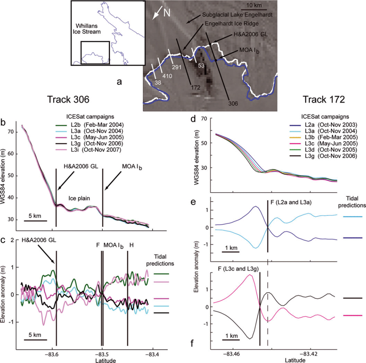
This example demonstrates the value of looking at the tide predictions concurrently with the elevation anomaly profiles. Additionally, it suggests that, although the DEM-based technique is a useful, relatively rapid method for determining the GL location around Antarctica, great care needs to be taken in regions of ice plains where the principal surface ramp is not a valid approximation for point G. However, the Reference Horgan and AnandakrishnanHorgan and Anandakrishnan (2006) technique has identified the coupling line in this region, which allows us to map the extent of the ice plain.
Retreat of Engelhardt Ice Ridge
In the Methods section, we attributed offsets between various maps of the GL location to differences in the techniques used to derive them. However, we cannot discount the possibility that the surface features defining the GZ may have actually moved between the sampling epochs for each satellite. In some areas, GL retreat is known to have occurred over quite short timescales (e.g. the GL for Pine Island Glacier retreated 1.2 ±0.3 km a−1 between 1992 and 1996 (Reference RignotRignot, 1998a)). The GL in the vicinity of Engelhardt Ice Ridge has also been observed to retreat rapidly (Reference Bindschadler and VornbergerBindschadler and Vornberger, 1998; Reference Fricker, Scambos, Bindschadler and PadmanFricker and others, 2007). Reference Fricker and ScambosFricker and Scambos (2009) showed that the ridge was retreating southward based on analyses of elevation profiles along ICESat track 53 (their fig. 4a). We examined the elevation profiles of four tracks that cross the ridge farther east of track 53(172, 291,410 and 38; see Fig. 5a for locations) and found that all indicate similar retreat. Two of these tracks (172 and 291) were sampled by a sufficient number of valid repeated passes that we could obtain estimates of point F at two epochs, allowing us to estimate a migration rate for point F.
For track 172, we estimated the location of point F based on two early (2003) repeated passes and compared this with the location from two later (2006) repeated passes (Fig. 5e and f, respectively). All of the repeated passes used in this analysis have cross-track separations of <75 m; thus, we expect errors from cross-track offsets to be small. The anomalies upstream of point F in Figure 5e are probably the result of the steep slope, and retreat, of the ridge. Based on the distance between ICESat point F in Figure 5e and f, we estimate this retreat rate to be ∼400 m a- 1 between 2003 and 2006. For track 219, we estimated a retreat rate of ∼450 ma−1 between 2004 and 2008 (not shown). These values are similar to a retreat rate of 330 ± 100 ma−1 between 2000 and 2005 from MODIS images presented in Reference Fricker, Scambos, Bindschadler and PadmanFricker and others (2007) (their fig. S2). Our estimates also compare well with the estimate of 447 ± 34 m a−1 between 1963 and 1992 by Reference Bindschadler and VornbergerBindschadler and Vornberger (1998), who compared US Department of Defense Declassified Intelligence Satellite Photography (DISP), Advanced Very High Resolution Radiometer (AVHRR) and Satellite Probatoire pour l’Observation de la Terre (SPOT) imagery.
These results indicate that GZ change can occur rapidly, so that great care must be taken when using different types of satellite datasets used to derive a single GL map: all data must be from, or adjusted to, a similar epoch.
Limitations and error assessments
Similar to the results of a study of the Amery Ice Shelf by Reference Fricker, Coleman, Padman, Scambos, Bohlander and BruntFricker and others (2009), we find four primary factors limit the success of this ICESat repeat-track analysis: (1) spacing between ICESat tracks; (2) surface roughness; (3) a small tidal range in the sampled set of tracks; and (4) persistent cloud cover. We discuss the effects of each of these limitations below.
The method we have described is fundamentally limited by the spacing between adjacent ICESat ground tracks, which increases from ∼5 km in the southern part of the RIS to ∼20 km in the northern portion of the ice shelf (Fig. 3). Also, because the ICESat tracks do not repeat exactly, the technique is affected by errors that arise from cross-track surface slopes (Reference Smith, Fricker, Joughin and TulaczykSmith and others, 2009). We have tried to minimize this effect by removing repeated passes that are offset >100 m from the reference track. Based on Figure 2, a conservative estimate of the error associated with cross-track surface slope is indicated by the scatter in the grounded ice elevation (0.3 m) divided by the surface slope in the GZ (2 m over 4 km); i.e., ∼600m.
Surface roughness such as crevassing introduces noise that compromises our ability to identify the tidal signal and thus to estimate GZ points F and H. The large outlet glaciers that drain the high plateau of the East Antarctic ice sheet through the Transantarctic Mountains to join the RIS (Fig. 3) create highly crevassed terrain. This is most evident in the vicinities of Mullock, Byrd and Nimrod glaciers (Fig. 3), where no GZ features could be identified where the glaciers meet the ice shelf. However, in the vicinity of Beardmore Glacier, points F and H were estimated continuously along the mouth of the outlet. This is presumably because the ICESat tracks at the mouth of Beardmore Glacier are parallel to (and typically do not cross) flowlines. In the vicinities of Mullock, Byrd and Nimrod glaciers, the tracks are almost perpendicular to the flowlines and crevasses. For these glaciers, the mapping of the GZ cannot be undertaken using our technique.
The other factors limiting the efficacy of ICESat repeat-track analysis are the persistence of cloud-cover in many of the areas of interest, and a small sampled tidal range. In particular, the outlet glaciers feeding the northern RIS are regions of persistent clouds, such that too few elevation profiles are available to clearly estimate points F and H. On the RIS, the tidal range is largest (>3 m) in the vicinity of Mercer Ice Stream and smallest (∼1 m) near Ross Island (Reference Padman, Erofeeva and JoughinPadman and others, 2003). Even for sections of the GL where the full tidal range is large, rejected data due to clouds and large cross-track offsets can lead to poor sampling of tidal range.
The highest absolute precision in locating points F and H that could be achieved by this technique is limited by the ICESat along-track footprint spacing (200 m after resampling). However, larger errors arise for the four reasons described above. The potential error in estimating point H is higher than that for estimating point F. This is because the gradients of the elevation anomaly profiles tend to change abruptly at point F but often only slowly tend toward zero at the hydrostatic point, making the estimation of point H less certain than the estimation of point F (see Fig. 2b). The error for points F and H is exaggerated when the track angle is oblique to the GL.
The effective uncertainty in estimating point F thus depends on the particular repeated passes chosen for the analysis (see Fig. 2b). To reduce this effect, throughout this study we have attempted to obtain the highest signal-to-noise ratio by choosing the repeated passes that represent the maximum tidal range. To quantify the impact tidal range can make, we estimated the locations of points F and H using two different pairs of repeated passes for the example track shown in Figure 2: lasers 3c and 3f (displaying the minimum tidal range) and lasers 3d and 3g (displaying the maximum tidal range). The difference between the locations based on these two pairs was ∼500 m along-track for point F and ∼1000m for point H. We repeated this process for seven other tracks that were nearly normal to the MOA GL, in regions of moderate tidal range. The tracks were chosen such that all repeated passes were close to the reference track, and were unaffected by cloud cover. We measured the along-track distance between the locations of points F and H based on pairs of repeated passes displaying the maximum and minimum tidal range. The differences ranged from 200 to 540 m for point F, and from 1000 to 3000 m for point H. From these analyses we assign typical errors for ICESat estimations of points F and H of ∼400 and ∼2000m, respectively, but note that more precise error estimates can be made on a track-by-track basis.
For comparison, Reference Horgan and AnandakrishnanHorgan and Anandakrishnan (2006) estimate a 1–2 km error in their location of the GL, and Reference GrayGray and others (2002) report errors of 1–2 km for their InSAR-based location of point F for sections of the GZ that are well resolved by InSAR. Reference GrayGray and others (2002) did not estimate position errors for poorly resolved sections of the GZ (the dotted sections of the Gray2002 GL in Fig. 4). However, we have shown that in some cases the offset between various combinations of the Gray2002, H&A2006 and MOA estimates of the GL location, and the ICESat location of point F, can exceed 10 km, which is significantly greater than expected offsets from the cited error estimates.
Conclusions
We have mapped the GZ of the perimeter, islands and ice rises of the RIS using ICESat laser altimetry. The landward limit of tidal flexure (point F) and the hydrostatic point (point H) have been estimated at 491 locations where repeated passes of ICESat tracks cross the GZ. We have compared the ICESat-derived GL, associated here with point F, with the same feature derived from InSAR. We have also compared it with the GL obtained from two ‘static’ methods: manual tracking of surface shading features in MOA imagery (Reference Scambos, Haran, Fahnestock, Painter and BohlanderScambos and others, 2007), and slope analysis of a high-resolution DEM (Reference Horgan and AnandakrishnanHorgan and Anandakrishnan, 2006). Both of these static methods exploit the fact that the ice surface slope near the GL usually changes rapidly as the basal stress decreases at the GL. However, the static methods sometimes identify different surface slope features from the complex surface topography typical of coastal regions of the ice sheet.
Our results demonstrate that no single method can provide an accurate, continuous map of the key GZ features for all of Antarctica. Each method has significant limitations and identifies different features within the GZ. We have shown that ICESat repeat-track analysis can accurately estimate points F, H and Ib along the track, but adjacent tracks are several km apart. InSAR provides accurate, quasi-continuous locations of points F and H. However, InSAR coverage is not complete, some regions lack the image-to-image coherence required to calculate ice motion, and some InSAR datasets (e.g. the ERS tandem mission) have inadequate sampling of the tidal range (Reference Fricker, Coleman, Padman, Scambos, Bohlander and BruntFricker and others, 2009). Analyses of surface slopes in high-resolution DEMs and satellite image products provide continuous estimates of GL location but rely on assumptions relating these surface features to the basal point G. For the RIS, the difference in the estimated location of the GL between methods is sometimes of order 10 km, with a maximum of ∼60km. These uncertainties lead to large errors in parameters describing the role of ice shelves in the climate system (e.g. the ice mass flux across the GL).
For some sections of the GL, the differences in location arise through errors in the analyses or limitations of each technique. In these cases, an improved GL map can be created by judicious merging of the most reliable sections from each dataset, or by reanalysis of a specific dataset guided by data from other satellites. For example, the discrete locations of F points from ICESat analyses could be used to constrain the selection of image features used to track the GL in MOA or LIMA imagery. However, in some regions the use of static methods can lead to misidentifications of the coupling line landward of an ice plain as the break-in-slope associated with the GL. Dynamic methods that identify point F could then be used to define the extent of the ice plain. Other permutations on the idealized GZ structure represented by Figure 2 are also possible, and can only be identified through the simultaneous analysis of several satellite datasets providing locations of specific GZ features.
We conclude that use of dynamic techniques to identify the location of GZ features through ICESat repeat-track analysis significantly improves our knowledge of the location of the GL and structure of the RIS GZ beyond what can be achieved with other satellite-based techniques. The most precise mapping of locations of points F and H is generally provided by differential InSAR imagery; however, in places where InSAR is not available it might be possible to accurately map GZ feature locations through synergistic use of ICESat repeat-track analysis and a static image-based method based on MODIS or LIMA imagery. Our results from the RIS will be incorporated into the Antarctic Surface Accumulation and Ice Discharge (ASAID) database, an International Polar Year project that includes determining the precise location of the GL for the entire continent (personal communication from R.A. Bindschadler, 2009). ASAID will contribute toward a benchmark dataset that can be used to monitor future changes. More accurate GZ maps will also improve inputs to numerical models of ice shelves, including ice-flow and ocean models, which are urgently needed to understand the processes that control ice-shelf evolution and how these relate to climate.
Acknowledgements
This work was supported by NASA grant NNX06AH39G to Earth & Space Research (subcontract to Scripps Institution of Oceanography). We thank NASA’s ICESat Science Project and the US National Snow and Ice Data Center for distribution of the ICESat data (see http://icesat.gsfc.nasa.gov and http://nsidc.org/data/icesat). This is Earth & Space Research contribution No. 129.


