


1. Introduction
1.1 Why we drill ice cores
Deep ice core drilling projects are usually undertaken for the purpose of climate reconstruction, which was first demonstrated by Dansgaard and others (Reference Dansgaard, Johnsen, Møller and Langway1969). The reconstruction of the past climate from ice core samples assumes that the snow in the ice sheet interior does not melt, and that annual layers accumulate horizontally, which leads to a continuous record (Cuffey and Paterson, Reference Cuffey and Paterson2010). The ice flow history can influence the reliability of ice core records and must be considered when reconstructing climate from ice cores (e.g. Jansen and others, Reference Jansen2016). As ice flows, the stratigraphic layers may be disturbed, which can lead to climate reconstruction errors, in particular for the deep parts of the ice column (Dahl-Jensen and others, Reference NEEM community members2013). Nevertheless, the visualization of stratigraphic deformation offers the possibility to decode past deformation in the bottom part of the ice sheet and to reconstruct ice core orientation.
1.2 Northeast Greenland Ice Stream and EastGRIP drill site
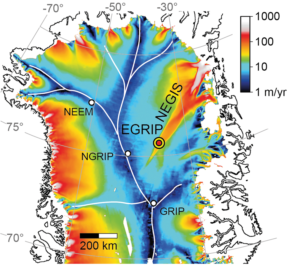
The East Greenland Ice Core Project (EastGRIP or EGRIP) ice core is drilled in northern Greenland (Fig. 1), at 75 38′N, 36 00′W, 2704 m a.s.l. (Vallelonga and others, Reference Vallelonga2014). This is a central location in the onset region of the Northeast Greenland Ice Stream (NEGIS). The NEGIS extends for more than 600 km almost from the ice divide to the coast. Unlike many ice streams where ice is entering the trunk of fast flow by a tributary system, the ice entering the NEGIS passes through the well-developed shear margins (Fahnestock and others, Reference Fahnestock, Abdalati, Joughin, Brozena and Gogineni2001; Joughin and others, Reference Joughin, Fahnestock, MacAyeal, Bamber and Gogineni2001). At the drill site the ice on the surface flows with 55 m/a in an ~10 km wide central flow band (Hvidberg and others, Reference Hvidberg2020). Observations by Christianson and others (Reference Christianson2014) indicate soft and deformable subglacial sediment in the vicinity of the NEGIS, which facilitate sliding as well as a connection of the shear margins’ positioning to the subglacial hydrology. Observations by Franke and others (Reference Franke2020) support these findings and indicate the existence of subglacial landforms, shaped by the activity of the ice stream.
Surface velocity map of northern Greenland on a logarithmic scale. Locations of the EGRIP drill site in the upper part of NEGIS and other selected ice core drill sites on ice divides (white lines). NEGIS extends almost from the ice divide, Southwest of EastGRIP, to the coast. Surface velocities were obtained from the MEaSUREs velocity data set (Reference Joughin, Smith, Howat, Scambos and MoonJoughin and others, Reference Joughin, Smith, Howat, Scambos and Moon2010a, Reference Joughin, Smith, Howat, Scambos and Moon2010b, same as used by Bons and others, Reference Bons2018) with data from the years 2000–2008.
1.3 Determining ice core orientation
In the visual stratigraphy images from EastGRIP, milky, impurity rich layers, known as cloudy bands, are found. These were observed and described for the first time by Gow and Williamson (Reference Gow and Williamson1971) in Antarctica and Hammer and others (Reference Hammer1978) in Greenland. These cloudy bands are only visible in ice from the last glacial period, i.e. below a depth of 1375 m (Mojtabavi and others, Reference Mojtabavi2019). All previously drilled ice cores in Greenland show cloudy bands (Faria and others, Reference Faria, Freitag and Kipfstuhl2010), but at EastGRIP, rapid changes from perfectly flat cloudy bands in one sample, to significantly folded layers in the next sample, were unexpected and unprecedented. These changes tend to occur at core breaks between two samples (sample length: 165 cm), collected in a single drill run. Thus, these features could be a result of randomized and irregular core rotation occurring each time a core section was drilled.
During the process of core recovery, the orientation is lost due to rotation of the drill. See Johnsen and others (Reference Johnsen2007) for a thorough description of electromechanical ice core drilling. Attempts to preserve this orientation, e.g. by using a spring to guide the drill, failed to work so far (Trevor Popp, pers. comm.).
Borehole logging to determine borehole inclination (also referred to as plunge) and azimuth direction (also referred to as plunge direction) is common practice in ice core and rock drilling. For many methods, it is the first necessary step to retrieve core orientation. Further mechanical devices are required to orient the core fully (Davis and Cowan, Reference Davis and Cowan2012). From rock drilling, many methods for reorienting a core are known. Methods such as ‘the spear’, sending a heavy spear with a sharp point or wax-pencil tip downhole after every run that marks the bottom edge of the core (Davis and Cowan, Reference Davis and Cowan2012), were not used in ice core drilling due to lack of time in the short drill season in summer and concerns about damage to the ice sample. Furthermore, this method only delivers relaible results in boreholes with an inclination greater than 15°. Many newer methods have evolved over the last decades, such as, Ezy-Mark, Ballmark, and Reflex systems, but have not been applied to ice core drilling. Paulsen and others (Reference Paulsen, Jarrard and Wilson2002) describe reorienting features using a downhole camera and matching these to features in the drill core. This is not applicable to EastGRIP, as there are no images of the borehole so far. Downhole imaging has been applied to the upper part (top 630 m) of the North Greenland Eemian Ice Drilling (NEEM) ice core, but not used for determining orientations (Hubbard and Malone, Reference Hubbard and Malone2013).
First oriented ice cores were drilled with a thermal drill at Vostok Station in 1972 (Talalay, Reference Talalay2020). A horizontal bolt was screwed near the thermal head and melted a groove on the core surface during drilling. An inclinometer section was embedded in the meltwater tank. Like this, three oriented core sections, of ~1 m each, were recovered. This method works well with thermal drills, as there is no internal rotation of drill sections. It becomes more complicated with electromechanical and thermal cable-suspended drills as the bottom drill parts rotate while drilling.
Recording azimuth and inclination of the non-rotational drill parts at the moment of core breaking are suggested by Talalay (Reference Talalay2014). This provides the spatial position of the pressure chamber, which can be related to the rotational parts of the drill section, thus retrieving the core orientation. Fitzpatrick and others (Reference Fitzpatrick2014) applied this idea and retrieved core orientations relative to magnetic North, which were marked using an azimuth line on the core just before extraction from the drill barrel. These marks did not always line up, either due to rotation of the core in the core barrel (Fitzpatrick and others, Reference Fitzpatrick2014) or due to problems with the azimuth measurements (Pavel Talalay, pers. comm.).
1.4 Motivation
In this study, we introduce a new method to determine ice core orientation. The main innovation is the usage of geological drilling know-how, such as the combination of borehole inclination with the apparent layer dip and applying this to directional features visible in ice cores. This is the first time, that directional features are used for thorough and complete reconstruction of ice core orientation.
To understand the flow of ice, we depend on directional information. The spatial orientation of large-scale radar images, showing the ice sheet's internal structure, is linked to the flight or ground path from which they were acquired. Thus, the direction can readily be implemented. However, due to the loss of ice core orientation during core recovery, all measurements done on an ice core are interpreted without directional information. However, this information about an ice core's orientation is crucial and a necessity for interpreting physical and flow properties of ice, and all other image data taken from the ice core. If the orientation is known, ambiguous observations are avoided, which allows for a more confident interpretation of the data.
As drills that preserve or record ice core orientation for the entire core have not been applied yet, other methods are required to determine core orientation. The method presented here supplies a technique, independent of the relative orientation obtained during logging by core break-matching (discussed later) and independent of stereographic projections of c-axis distribution (Weikusat and others, Reference Weikusat2017, also discussed later). We determine the orientation of 451 samples from 1375 to 2120 m depth, i.e. ice from the last glacial period (Mojtabavi and others, Reference Mojtabavi2019), characterized by the occurrence of cloudy bands (Hammer and others, Reference Hammer1978). These cloudy bands are necessary for the application of the method, as well as a certain amount of flow, to detect directional deformation. Additionally, some borehole inclination is necessary, as this method will not provide results in a perfectly vertical borehole, which would be a rare case in the electromechanical ice core drilling. We then compare our results to core break matching and c-axis orientations, for verification of our method.
2. Methods
2.1 Journey of an ice core – from the bottom of the ice sheet to the measurement table
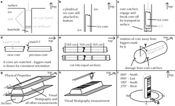
During drilling and core preparation, many steps change the orientation of the sample before measurements are made. The drill (Fig. 2a) cuts a cylinder out of the ice, with the bottom still attached to the bulk ice (Fig. 2b). The core catchers engage the ice, and the pull of the winch breaks the cylinder of ice off the bottom. The length of this cylinder, obtained in one run, can be up to 3.6 m, depending on core barrel length. It is then lifted to the surface (Fig. 2c), while the drill and core barrel rotate freely, and the in-situ core orientation is lost.
Steps to recover an ice core until the measurement of visual stratigraphy (a to h). Spatial orientation of the direction of view, defined here as δ, is measured clockwise from North (i).

When the core reaches the surface, its top is matched to the bottom break of the previous ice core section (Fig. 2d). In most cases, this match is possible, thus retrieving the relative orientation of the drill core. The logger's mark, a continuous line on the core, represents this relative orientation. For ease of handling, the core is cut into regular sample lengths, e.g. 165 cm pieces at EastGRIP (Fig. 2e).
In cases of shattered ice, core quality is affected and samples are rotated to provide undamaged ice for all necessary measurements. It is rotated relative to the line marked on the core (γ, Fig. 2f).
Now two cuts are made along the long axis of the core (Fig. 2g). This provides three 165 cm-long pieces, one for physical properties measurements, one for visual stratigraphy and most other measurements, and one as an archive piece for future purposes. The visual stratigraphy sample is created by an optical 2D scan from the top (Fig. 2h) while being illuminated from below. Figure 2i illustrates the spatial orientation of the ice core, described as δ from now on. It is measured clockwise from geographic North.
2.2 The line scanner
The line scanner, used at EastGRIP, has been developed by Schäfter+Kirchhoff GmbH, in cooperation with Alfred Wegener Institute, Helmholtz Centre for Polar and Marine Research (AWI). Details can be found in, e.g. Svensson and others (Reference Svensson2005) or Faria and others (Reference Faria, Kipfstuhl and Lambrecht2018). On Greenland, the line scanner was applied to obtain a line scan profile for sections of the NEEM deep ice core during the field campaign seasons 2009 to 2011 (unpublished data). An older version of this device was used for the drilling campaign at the Northern Greenland Ice Core Project (NorthGRIP), in the 2000s Svensson and others (Reference Svensson2005). At NorthGRIP, the line scan was only done on the second NorthGRIP core, below 1300 m. The first visual archives of an ice core from Greenland were created on the Greenland Ice Core Project (GRIP) and the Greenland Ice Sheet Project (GISP2) ice cores in the 1990s, in an enormous effort, using pencil and paper (Grootes and others, Reference Grootes, Stuiver, White, Johnsen and Jouzel1993; Alley and others, Reference Alley1997).
Faria and others (Reference Faria, Freitag and Kipfstuhl2010) and Jansen and others (Reference Jansen2016) show the potential of visual stratigraphy images, e.g. complementary to other methods for deciphering deformation mechanisms, novel for identifying structures in ice such as tilted-lattice bands. Other applications are stratigraphic dating of ice cores, as done by, e.g. Svensson and others (Reference Svensson2005).
To acquire the line scan images, a polished slab of ice is illuminated at an angle from below, often referred to as ‘dark field’ imaging. Impurities, dust, bubbles, and fractures will scatter the light, thus making these features visible. While the core is illuminated, a camera scans the surface and detects areas where light is scattered (Fig. 2h). Where light travels through ‘clean’ ice and is not scattered, a dark field below the ice core is detected (Svensson and others, Reference Svensson2005; Faria and others, Reference Faria, Freitag and Kipfstuhl2010). The main cause of light scattering in ice from the last glacial period, other than fractures, is cloudy bands. These are layers with a high mineral dust concentration (Hammer and others, Reference Hammer1978), and micro-inclusions (Faria and others, Reference Faria, Freitag and Kipfstuhl2010).
2.3 Borehole logging
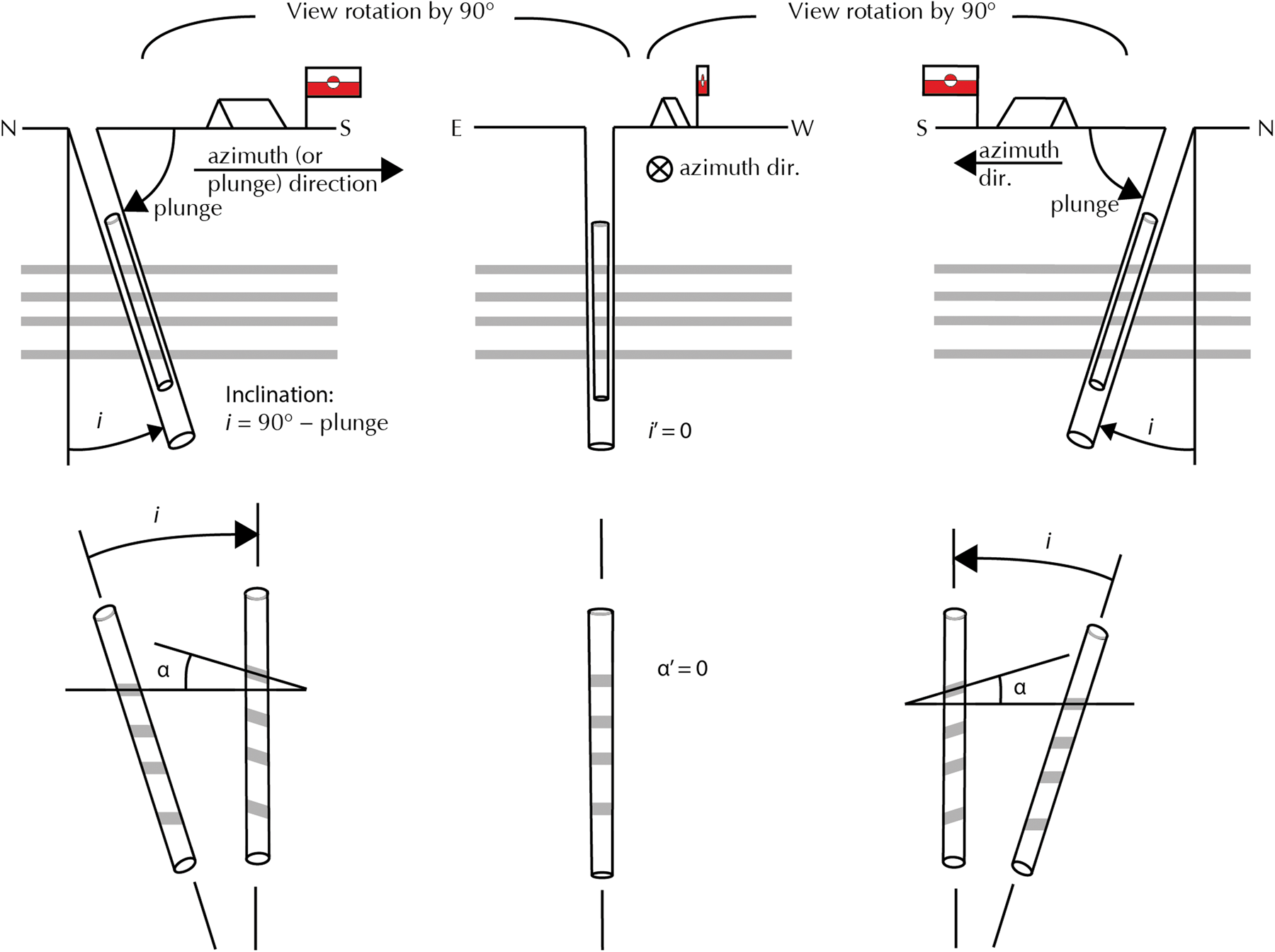
The Danish Borehole Logger (Gundestrup and others, Reference Gundestrup, Clausen and Hansen1994) provides the boreholes inclination and spatial azimuth orientation. The inclination (i) of a borehole can be defined as the angle between the vertical and the borehole axis, or its plunge, which is the angle it makes with the horizontal plane (Fig. 3). The plunge (or azimuth) direction is the geographic direction in which the borehole points when projected on the horizontal plane. For consistency, we will from now on refer to plunge direction as azimuth direction (φ). We use the convention that N = 000°, E = 090°, etc., up to 360° = 000° (Fig. 2i).
Three viewing directions of the same borehole. In the top row, the angles i and i′ represent the true and apparent borehole inclination (90° − plunge), respectively. i and i′ in the bottom row are the angles necessary to tilt the ice core to vertical. Assuming horizontal layering, i is equal to α, the dip angle of inclined layers in the ice core and i′ is equal to α′, the apparent dip angle.
In this study, we do not include other measurements by the logger (temperature, borehole diameter, and liquid pressure). The EastGRIP borehole has been drilled with inclinations up to 6° from vertical. The borehole is logged at the beginning and end of every field season with the purpose of observing undisturbed borehole temperatures, changes of diameter, and borehole geometry due to ice deformation. The measurements from the end of the 2019 field season are used here.
2.4 Tilt of cloudy bands due to borehole tilt
An observer looking at an arbitrarily oriented borehole will see an apparent inclination of i′ = 0° (or a vertical plunge of 090°) when looking in the borehole azimuth direction, or in the opposite direction (Fig. 3 middle). Any other viewing direction results in an apparent inclination between 0° and the true inclination, when the viewing direction is ± 090° to the azimuth direction (i′ = i, Fig. 2, left and right). The same is observed when considering the tilt of layers (usually cloudy bands) in an extracted drill core.
The orientation of the true horizontal plane in a core is not known if the core is not oriented and, therefore, only its inclination and azimuth direction are known. We therefore define the horizontal in a core as the plane perpendicular to the core axis. When the core transects layering at an angle less than 090°, layering will appear tilted. The true tilt α will only be observed when looking at the core perpendicular to the material line in the core that was originally parallel to the plunge direction. The observed tilt α will then be identical to i, but with opposite sign. Here we use the sign convention that α is positive when layers appear to be tilted clockwise, i.e. to the right. When the core is observed from an arbitrary direction, the layers will have an apparent tilt angle α′, which can range from − i to + i.
2.5 Measuring a cloudy band's tilt
We automatically measured the layer tilt of all 451 visual stratigraphy samples (equivalent to 745 m of core) using Matlab (MATLAB, 2018). Other methods for measuring a layer's tilt are discussed later. We created a brightness-intensity profile along the left and right sides of each image. Bright sections caused a peak in the signal and dark sections valleys. Using the built-in function for signal processing, ‘alignsignals’ the offset (D) of the left and right brightness-intensity curves was determined. With a known distance between the left and right side (x), the angle is calculated with simple trigonometry:

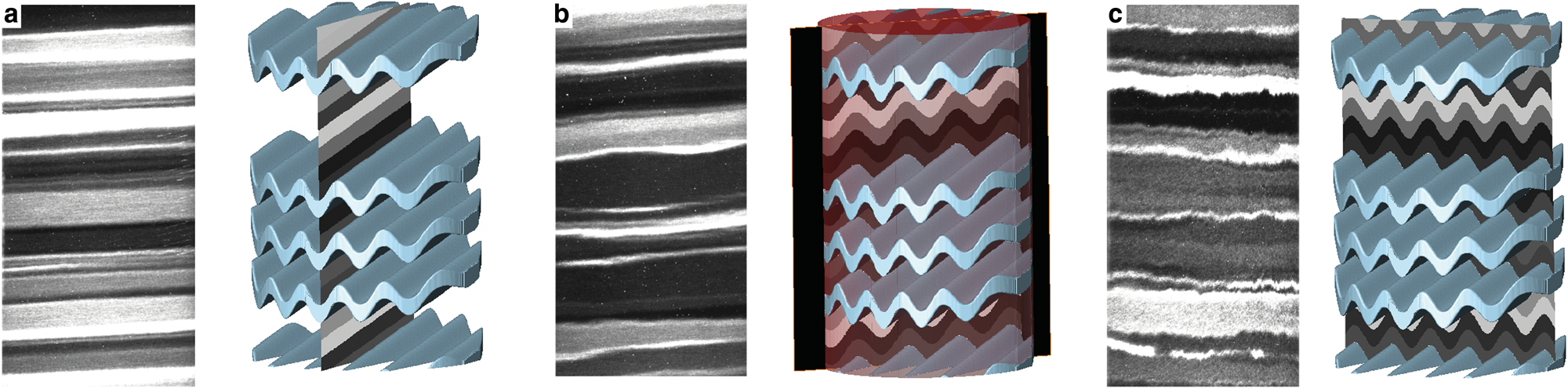
Manual verification was necessary because irregularities in the layers may prevent the proper alignment of the same layer. In the samples, we observe three types of layering. Straight, regular layers with (Fig. 4a), long wavelength undulations (Fig. 4b), and small-scale folds with approximately vertical axial planes, termed crenulations in geology (Cosgrove, Reference Cosgrove1976, Fig. 4c). Crenulations form by lateral shortening of thin laminations in rocks or a foliation defined by strongly anisotropic minerals, such as micas (Cosgrove, Reference Cosgrove1976; Ran and others, Reference Ran2019) or ice (Bons and others, Reference Bons2016).
Three types of deformation features. (a) No features and flat layering, (b) long wavelength undulations, and (c) crenulations (symmetric upright folds), overprinting other features. Visible structures depend on direction of view, illustrated by the cylinder with several folded layers next to every image.
The automated method for tilt measurements was verified manually on 30 random samples. It provides good (± 0.1°) results on featureless layers (Fig. 4a), but the measured tilt scatters in case of samples with folded or undulating layers (Fig. 4b). Using the median of up to 288, tilt measurements on one sample delivered results very similar (within ± 0.3°) to manual measurement. All angles greater than 8° (or smaller than − 8°) were removed after manual verification that no layers have such a large inclination.
2.6 Reconstructing the core orientation
Figure 5 illustrates terms explained in the following section. The tilt or dip direction (labeled as ‘dip dir’) is the direction of the steepest inclined line on a tilted plane. The dip angle (α) is the declination of this plane, measured from a horizontal projection ($\overline {MA}$ ). The angle α is the largest possible plunge angle of a line on this plane. Strike is the unique non-inclined line on an inclined plane. Dip direction is 90° to strike and when viewed from the top, as in Fig. 5a (right), $\overline {MA}$
 and ‘dip dir’ have the same orientation.
(a) An inclined plane (gray square), e.g. a layer in an ice core, with the dip angle α on the steepest profile $\overline {MA}$ . Same dip of gray layer, but smaller apparent dip angle α′ on profile $\overline {MA'}$
 . Profile $\overline {MA'}$
 is β away from strike. For one apparent dip angle α′ there are four possible positions for β, spanning profiles from M to A’, A”, B’, and B”. (b) Ice core (blue circle) viewed along the vertical axis. Surface of ‘cut 2’ (Fig. 2G) is either along $\overline {A'B'}$
 or $\overline {A''B''}$
 . δ(1−4) represent the possible viewing directions. All red lines, extended vertically, could be possible image planes.
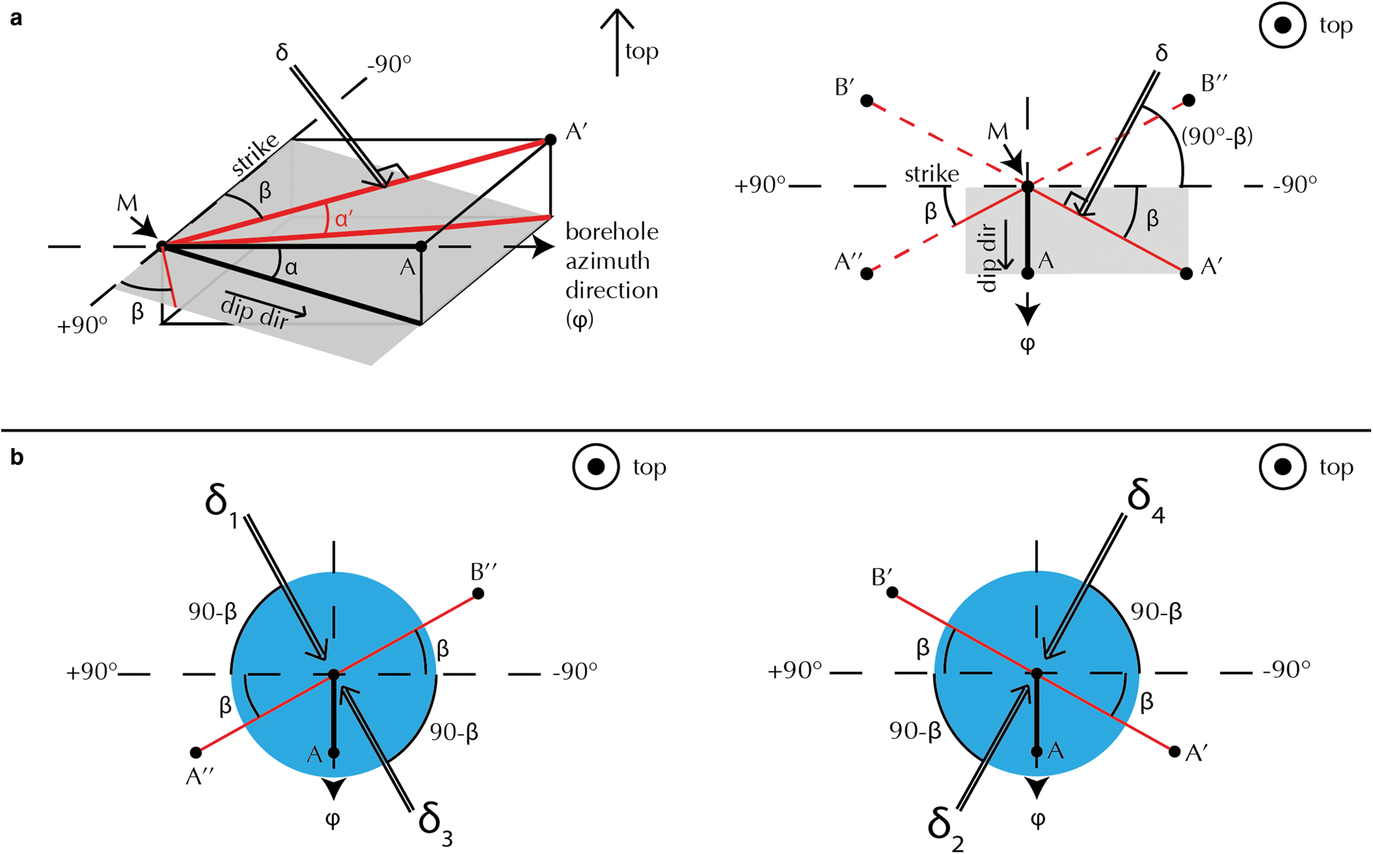
The apparent dip (α′) is the dip angle that is actually observed when a core is sectioned. Apparent dip direction (Fig. 5, red line $\overline {MA'}$ ) is the geographic orientation of this intersection on a horizontal plane. α′ ranges between α and 0 (absolute values). For further details about apparent dip consult, e.g. Fossen (Reference Fossen2016). The dip direction relative to strike, of any apparent dip angle α′ is given by β:

In our case, α is given by the maximum inclination of the borehole (i, Fig. 3) and α′ represents the measured tilt of a cloudy band in a visual stratigraphy sample. The angle β is defined as the angle between the strike and the intersection of the section and horizontal plane, $\overline {MA'}$ (red line in Fig. 5). It is also the angle between strike and $\overline {A'B'}$
 and $\overline {A''B''}$
 . The lines $\overline {A'B'}$
 and $\overline {A''B''}$
 extended as planes parallel to the ice core axis, and are two possible section orientations for a given angle β (Fig. 2g). Visual stratigraphy is scanned from a 90° angle to the section plane (Fig. 2h). For such a given angle β, these two planes can be viewed from two opposite directions, giving a total of four possible viewing directions δ(1−4):


The borehole azimuth direction (φ) was logged at the end of the 2019 field season and is required to determine the other angles that link the coordinate system from Fig. 5 to a fixed geographical orientation, as in Fig. 3.
δ(1,2) have a positive layer tilt (downward sloping to the right), both are on the + 90° side in Fig. 5, bottom panel. Negative tilts (to the left) are represented by δ(3,4), lying on the − 90° side. Knowing the sign of the layer tilt reduces the number of possible orientations from four to two, as either Eqn (3) or (4) would apply.
We will show that δ(1,2) (or δ(3,4)) are connected to the type of deformation structure seen in the visual stratigraphy. This makes each δ unique to distinguish and enables the reconstruction of the true direction of view.
3 Results
3.1 Input parameters for EastGRIP core orientation reconstruction
The analyzed samples range from a depth of 1375 to 2120 m. We measured the tilt of cloudy bands (α′) for every visual stratigraphy sample, and plot one point per 165 cm-long sample (Fig. 6a). Measured layer tilts vary between − 4° and + 4°, and are randomly distributed. In Fig. 6a, some clusters are visible and these will be discussed later.
(a) Tilt of cloudy bands (α′) from 1375 to 2120 m (bag 2500 to 3856), each circle is the median value of 288 measurements for each 165 cm-long sample. (b) Inclination i and (c) azimuth direction φ of the EastGRIP borehole against depth. Inclination angle from (b) also shown as a thin line in (a).

The borehole inclination i ranges from 2.7° to 3.6° (Fig. 6b). Assuming horizontal layers in the ice sheet, i of the borehole is equal to the maximum layer tilt α in the ice core (Fig. 3). For i = 3.5°, we expect to see an apparent layer tilt α′ ranging from 0 to ± 3.5°, depending on the viewing direction.
In the analyzed depth range, the borehole azimuth direction ranges from 190° to 150°, meaning it shifts from plunging towards south to a southeast direction (Fig. 6c). This information is the input for Eqns (3) and (4) to retrieve an absolute orientation for the ice core.
3.2 Deformation structure matched to layer tilt
To differentiate the two potential δ, we make use of observed deformation structures, as explained above (Fig. 4). When plotting the cloudy band's inclination against depth, color-coded for specific deformation structures, a systematic arrangement is visible (Fig. 7). Above 1900 m, the flat layers with no features (Fig. 7a, mean as dashed line) are located at the high and low values of the tilt. In the same depth range, cloudy bands with crenulations (Fig. 7c) have values closer to 0°. Cloudy bands with long-wavelength folds and undulations (Fig. 7b) scatter over the full spectrum of layer tilts.
Deformation-structure types and the corresponding layer tilt of cloudy bands against depth. Cloudy bands with no or flat features (a, blue), long wavelength undulations and folds (b, red), and crenulations (c, orange). Dashed lines are means for 1375 to 1900 m separated for positive and negative tilt. No features mean: ± 2.3 and crenulations mean: ± 1.6.
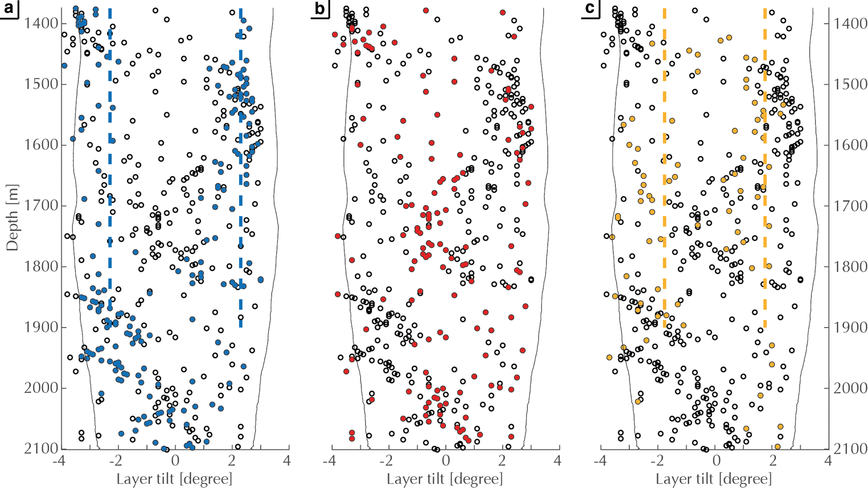
Borehole inclination and azimuth direction change significantly below 1900 m (Fig. 6). The tilt of layers with no features (Fig. 7a) gradually shifts to values around 0°. Layers with crenulations (Fig. 7c) now incline at larger values. Thus, these specific deformation features are linked to specific layer tilts.
3.3 Work flow diagram
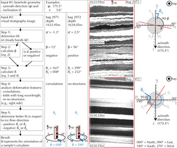
The flow diagram (Fig. 8, left side) supplies the user with a step-by-step instruction on how to use the presented method. It requires the input of borehole geometry (#1) and visual stratigraphy images (#2), and knowledge about ice flow direction (step 5). All other parameters are obtained from these. In the following, to illustrate the method, two consecutive visual stratigraphy images from a depth of around 1634 m (bag 2971 and 2972), with different deformation structures, are compared and reoriented (Fig. 8, right side).
Left: flow diagram to determine ice core absolute orientation, applied on bag 2971 and 2972. Middle: visual stratigraphy images of the two consecutive bags, including a depth scale. Right: sketch of visual stratigraphy plane, including relevant angles to obtain the orientation. Blue: spatial orientation of δ. Red: visual stratigraphy plane.

Input #1 defines the reference system, i.e. the azimuth direction and inclination of the borehole. Azimuth direction φ is 175.5°, and borehole inclination i is 3.6° for bag 2971 and 2972. Thus, this is also the dip direction and dip angle of our layers.
The apparent dip α′, i.e. the visible tilt of the layers, in bag 2971 and 2972 is − 1.3° and 2.5°, respectively. We apply Eqn (2) to calculate β, which is 12° and 56°, respectively. For a negative layer tilt α′, Eqn (4) is used for bag 2971. For the positive tilt α′ in bag 2972, we apply Eqn (3). Both provide two possible viewing directions δ = 008° and δ = 163° for bag 2971 and δ = 232° and δ = 299° for bag 2972 (see Fig. 8).
In the visual stratigraphy of bag 2971, we can clearly identify crenulations, linked to compression folds, and thus, the direction of view for δ must be close to perpendicular to ice flow direction of NEGIS (flow towards 025°). In this case, the position at 008° fulfills this requirement. A viewing direction of 163° would not represent an angle where compressional folds would be visible in the stratigraphy, and can therefore be eliminated as a possible viewing direction.
Cloudy bands in bag 2972 show no deformation features. Thus, the cut plane must be oriented approximately parallel to flow direction. At δ = 232°, we would expect to see deformation features in the cloudy bands. The second option δ = 299° however, is closer to the anticipated value parallel to the ice flow direction. Therefore, the first value (232°) can be ruled out.
3.4 Comparison of viewing direction δ to other methods
3.4.1 Relative orientation from core recovery
Before cutting the ice core for visual stratigraphy analysis, it is rotated at an angle γ, relative to the loggers mark (illustrated in Fig. 2f). This rotation defines the relative core orientation γ, which is continuously documented (Fig. 9, red). We calculate the absolute orientation δ (Fig. 9, black) for all samples, which represents the orientation relative to geographic North. We observe a strong correlation in the difference of absolute and relative orientation δ − γ (Fig. 9, blue). Subtracting γ from δ determines the deviation of the loggers mark from geographic north (compare to Fig. 2).
(a) Absolute spatial orientation δ (black) and relative orientation γ (red) against depth. (b) δ − γ (blue) describes the offset angle of the relative orientation from geographic North. Vertical lines show core breaks where a match was not possible.
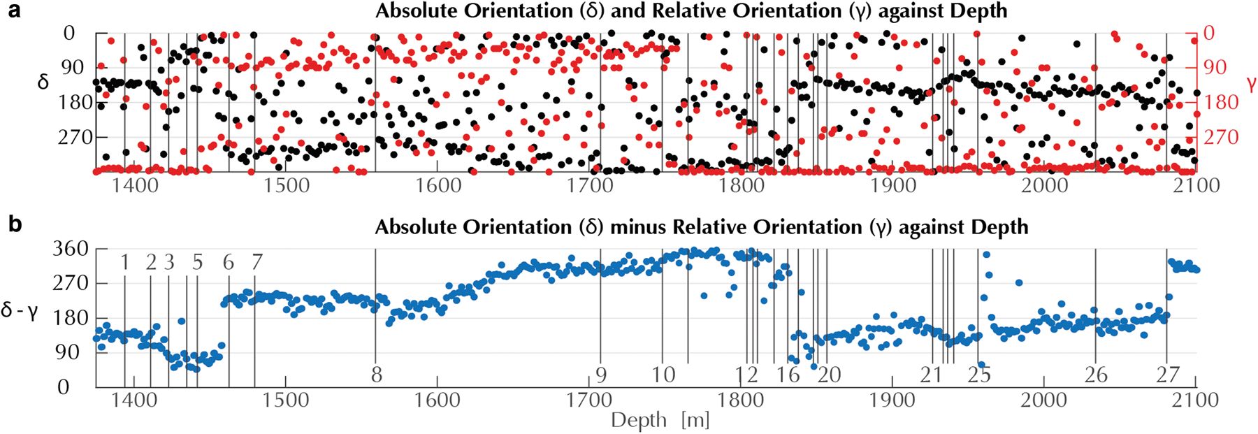
Figure 9 also indicates the loss of relative core orientation (vertical black lines) due to mismatches of core breaks (illustrated in Fig. 2d). For each mismatch in a core break, a new loggers mark is created, which has a random but continuous orientation for a range of matching core breaks. In sections with a preserved relative core orientation, very small rotations (of γ) are aimed for prior to cutting the ice core for visual stratigraphy. This results in many layer tilt measurements clustering around a certain value as this is the preferred cut orientation during core preparation.
All core mismatches in this section are documented in the field protocol as ‘probably lost’, except break number three, 16, and 19, which are labeled as ‘not-matched’. ‘Not-matched’ means that the relative orientation is lost, but the mismatches at breaks three and 19 do not show this mismatch in our data (Fig. 9). On the other hand, the mismatch at break 16 is clearly visible. In many of the assumed core mismatches, the orientation is, in fact, not lost (e.g. break one, seven, nine, and 26). A prominent example of a loss of core orientation is break 27, where the orientation (δ − γ) changes abruptly.
3.4.2 Orientation of crystal-scale directional features
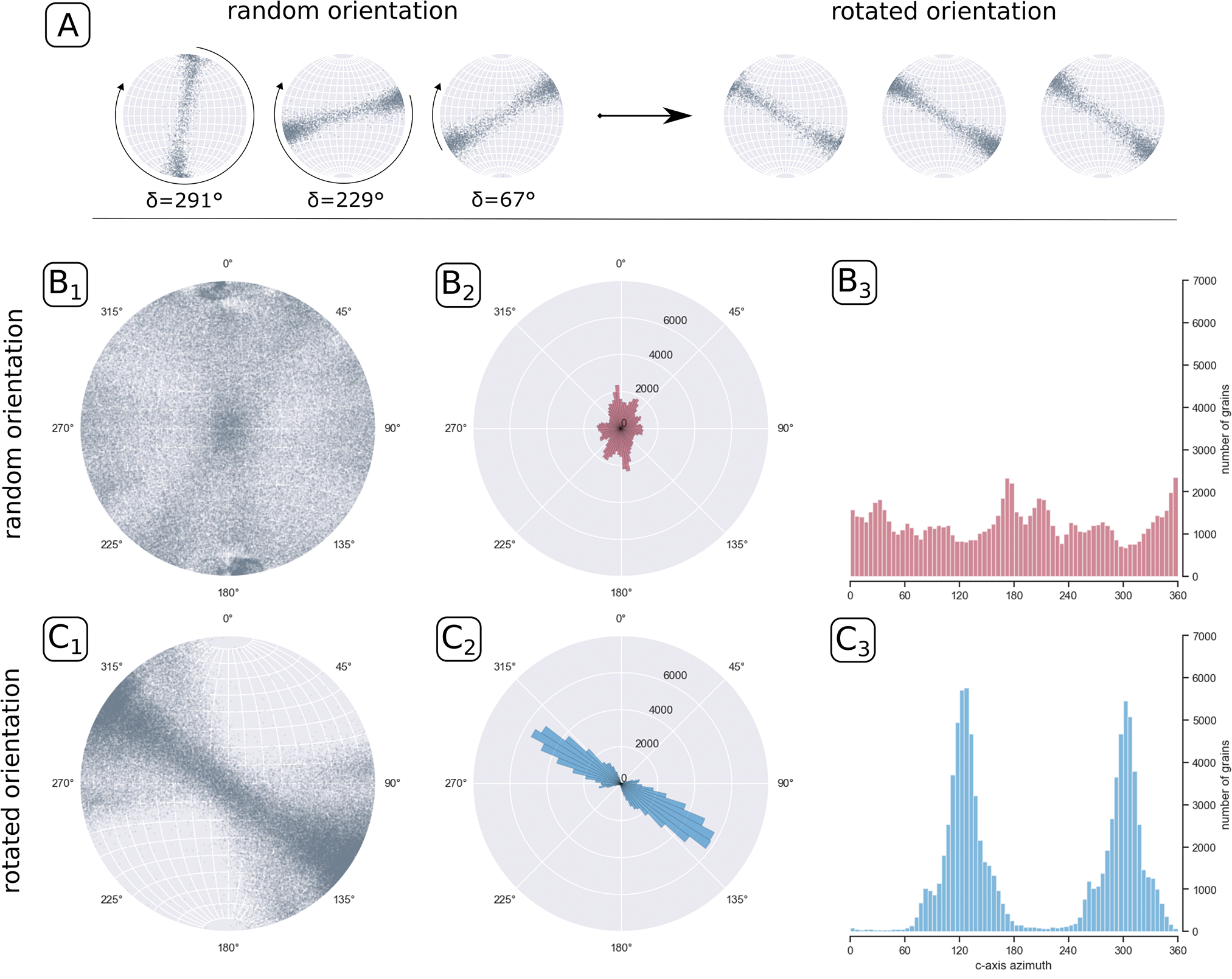
The orientation of a single ice crystal can easily be described by its c-axis, which is the vector perpendicular to the crystal's basal plane (e.g. Petrenko and Whitworth, Reference Petrenko and Whitworth1999). C-axis orientation has been measured continuously, every 10–15 m, throughout the EastGRIP core. Between 1375 and 2120 m, we use 34 c-axis plots. They show a c-axis distribution that is classified as a girdle in varying strengths.
Each projection alone shows a developed girdle with various orientations (Fig. 10a). These plots have a random orientation, when all are plotted together without rotational correction (Fig. 10b 1). This is also visible in the rose diagram and histogram (Fig. 10b 2,3). Each c-axis plot may be rotated by δ as determined by the method reported here (Fig. 10a). A systematic directional feature, i.e. a girdle with the same orientation for all samples, is visible when all samples are oriented (Fig. 10 bottom panel). The vertical girdle is now clearly orientated towards 120° and 300°, which is approximately perpendicular to the assumed flow direction at 030°.
Comparison of stereographic projections of crystallographic oriented fabric c-axis of an unrotated and rotated ice core. Panel (a) shows three individual stereographic projections before and after the rotation. A comparison of 34 c-axis data sets are shown in panels (b) and (c), with: (1) stereographic projections of the c-axis of all ice crystals, (2) a rose diagram, and (3) a histogram showing the distribution of the azimuth of all ice crystals binned in 5 degree units, respectively, before and after re-orientation.
4 Discussion
4.1 Statistical overview
Reorientation of the EastGRIP ice core worked well for 396 of 451 samples (88%). These 451 samples cover 745 core meters, which covers the full interval of interest from 1375 to 2120 m depth. After a comparison with the relative orientation γ, a good agreement was found for 441 of 451 samples (98%). In the remaining ten samples, the layer tilt is very close to 0°, so the sample can be viewed from two opposing sides, allowing two possible orientations, which cannot be distinguished further.
4.2 Cloudy band tilt measurement
The limited accuracy in measuring the inclination of a cloudy band is the largest source of uncertainty. The measurements in featureless samples are the most accurate, as every cloudy band is parallel to the one above and below.
As deformation of the visual stratigraphy increases, the accuracy of the tilt measurement declines. The approach by Drews and others (Reference Drews2012), who used the Hough transform (Hough, Reference Hough1962) on visual stratigraphy data from the European Project for Ice Coring in Antarctica, Dronning Maud Land Deep Drilling (EDML), was tested on our data. We added a pre-processing step to the Hough transform, using the built-in Matlab skeleton function for binary images, which greatly improved the outcome (MATLAB, 2018). The skeleton function finds the centerline between two edges, providing the average tilt of the top and bottom edge of a cloudy band. Still, a large number of detected lines in the image did not match stratigraphic layers. Therefore, for our approach, we determined a cloudy band's inclination by using left-right grayscale signal alignment (see method section).
Another approach for detecting the layer tilt is using fast Fourier transform. This method is suggested by McGwire and others (Reference McGwire2008) and applied on the West Antarctic Ice Sheet Divide Deep ice core (Fitzpatrick and others, Reference Fitzpatrick2014). However, it holds the same limitations as the Hough transform and our grayscale alignment, as undulations and folds in the cloudy bands scatter the result.
An increase of disturbances in the cloudy bands correlates with variations of layer tilt within one sample. The top edge of a cloudy band can have a different tilt to the bottom one, as the layer thickness can vary within the width of one sample (Fig. 8, cloudy band at 1633.98 m). This means that any method to determine layer tilt will suffer an increase in uncertainty the more the layers are disturbed. We therefore assume that the straightforward comparison between left and right sides of a sample suffices.
4.3 Relative and absolute orientation
To estimate the uncertainty in the tilt measurement, we compare the absolute orientation δ to the relative orientation γ. The latter was collected over three field seasons, by approximately nine different operators, and rounded to the next 5° or 10°, therefore, we expect a certain range of scattering. Figure 9b shows that the difference of absolute orientation minus relative orientation (δ − γ) align. If we assume γ to be very precise (to the closest 5°), the noise in this alignment is caused by inaccuracies in δ. Although there are uncertainties in tilt measurements of cloudy bands, the results show that the general orientation δ agrees with the relative orientation γ taken during ice core processing in the field.
The presented results are a rare opportunity to analyze the quality of core break matching (Fig. 2d) during ice core logging in the field. Mistakes made can be identified by comparing the relative orientation γ (Fig. 2f) to the absolute orientation δ. A loss of relative core orientation is indicated as a sudden change of δ − γ. Three of these are easily spotted between break five and six, at break 16, and break 27. While break 16 and 27 are located exactly at the change of angle, the change of angle at 1459 m depth is located 4 m above mismatch six. As this agrees well with the length of core retrieved in one drill run, we can interpret an inconsistency in documenting the depth while logging. This interpretation is most likely not valid for mismatch eight, where the small change in δ − γ is observed 7 m deeper.
An interesting feature is the slow shift of δ − γ between 1600 and 1650 m (from 210° to 300°). The relative orientation is assumed to have been kept constant and borehole inclination and azimuth barely change (Fig. 6). However, an observed gradual shift over 90° could be the sum of tiny shifts in orientation during ice core logging. We find inconsistencies in the loggers field protocol for this depth range, where although all core breaks are labeled as matched, smaller core sections are missing or out of place. This gradual shift of relative orientation could be the result of small core break mismatches, due to these missing or too small sections. A more apprupt change in δ − γ is observed between mismatch 11 and 12, where δ − γ decreases sharply and then returns to the previous level. Again, the loggers field protocol shows inconsistencies for this part of the core, however, without mentioning further details. We argue that the deviations of five samples after mismatch 25 are most likely related to an incorrect measurement of γ because the correlation works well before and after this section and no errors in the tilt measurements were found.
Problems with core break matching seem to cluster. They are located between mismatch 12 to 20 and 21 to 25. While this could be related to variations in the drill setup and difficulties in drilling, leading to a reduced core quality, it could also be related to personal preferences of the core logging operators.
In the cluster between mismatch 12 and 20 there are several occasions where a mismatch was assumed, but the orientation was actually preserved, e.g. at mismatches 12, 13, 14, and 20. The challenges for continuous and precise core break matching can be observed between mismatch 15 and 19, where the values show a large variability and two mismatches are labeled as ‘not-matched’.
There are many sections where core break matching worked very well. Between mismatch seven and eight, 20 and 21, and 25 and 27, δ − γ does not change over longer periods. Even with a number of different personnel acquiring the data, core break matching works very well in the analyzed depth region. The field protocol seems to be more on the conservative side, as at most of the mismatches labeled with ‘probably lost’ the relative core orientation is actually preserved. Also, the documentation of core rotation prior to cutting (γ, Fig. 2f) was done in an diligent manner, with very few exceptions.
4.4 Direction of flow inferred from the crystal orientation
The orientation distribution of the c-axes of crystals in one sample are called fabric, or crystal preferred orientation (CPO). When ice is deformed, the CPO changes, with its type depending on the dominating deformation mode (e.g. Kamb, Reference Kamb1972). The two main processes impacting the fabric pattern are (1) rotation of c-axes towards the direction of maximum finite shortening (Alley, Reference Alley1992; Qi and others, Reference Qi2019) and (2) recrystallization leading to the formation of new grains with different orientations, compared to the host grain (Llorens and others, Reference Llorens2017). Information on the deformational history can therefore, to a certain extent, be derived from the fabric of a sample (Kamb, Reference Kamb1972; Thorsteinsson and others, Reference Thorsteinsson, Kipfstuhl and Miller1997; Wang and others, Reference Wang2002; Montagnat and others, Reference Montagnat2014; Weikusat and others, Reference Weikusat2017).
According to Cuffey and Paterson (Reference Cuffey and Paterson2010), the observed developed vertical girdle between 1375 and 2120 m indicates extensional deformation along flow direction. If the dominating stress regime is axial extension, crystals rotate and basal planes shift towards paralelllism with the direction of extension (Thorsteinsson and others, Reference Thorsteinsson, Kipfstuhl and Miller1997; Wang and others, Reference Wang2002). Hence, c-axes rotate away from the direction of extension, producing girdle fabrics. Depending on their strength, patterns are classified as developing, developed, or strong girdle. The stronger a girdle, the more c-axes are aligned in the girdle, and the thinner the girdle becomes (Cuffey and Paterson, Reference Cuffey and Paterson2010).
The use of visual stratigraphy data enabled us to rotate the c-axis orientation data in a structured way. Doing so results in girdles that are aligned perpendicular to the observed flow direction of 030° of NEGIS. Our data confirm that the ice stream's extensional deformation results in a vertical girdle perpendicular to the flow direction.
Some scatter remains, which can be explained by unavoidable difficulties in measuring the angle of undulations and folds in stratigraphic layers and small-scale changes in the crystal fabric. However, the rotation of the fabric data using the correction we derived with our method turned out to be successful and indicates a deformation pattern, which agrees very well with the observed flow direction of NEGIS (Hvidberg and others, Reference Hvidberg2020).
4.5 Interpretation of visible deformation structures
The schematic image of folds in a cylinder, as done in Fig. 4, is an idealization, as it shows the gray-scale variation within an infinitely thin slice. Ice is a transparent material, and the image obtained in a line scanner is the product of light passing through a thick slice and is averaged over the focus depth. The sharpest image is obtained when layer boundaries align in the direction of observation. This is always the case in undisturbed layers. However, when layers are folded, this is only the case when looking along the fold axes. We therefore only observe sharp, thin layers with clear crenulation folds in sections at a large angle (δ around 025° or 205°) to the fold axis or extension direction. Cutting the folds obliquely results in more wavy patterns that may resemble extensional structures, such as boudins, shear bands, and truncations.
Field geologists are acutely aware that structures may look very different, depending on how they are intersected by the outcrop surface. The true nature and style of folds, for example, is only seen in surface that are approximately perpendicular to the fold axis. The same applies here. After having established the true orientation of all drill-core section, assuming a consistent fold-axis orientation, those sections that have the proper orientation can be selected to analyze the deformation structures. Care should be taken not to over-interpret other sections, as the oblique sections through structures may be misleading. A variation of cloudy-band morphology with depth could reflect a true variation in type or frequency of deformation structures. However, orientation of the drill-core sections should first be carried out to ascertain that this is not an artifact of sectioning. In the current case, it appears that variations that range from straight layers to folds can be explained by this sectioning effect. Approximately straight layering is observed in sections close to parallel to the flow direction, while folds are observed in those perpendicular to it. This is consistent with extension of the ice sheet in the direction of flow and lateral constriction, which is expected to result in the observed fold orientations (Bons et al. Reference Bons2016). The surface velocity fields at the EastGRIP drill site (Hvidberg and others, Reference Hvidberg2020) support this deformation regime as surface flow lines converge into the ice stream. Inside NEGIS the ice flow is parallel and the velocity is a magnitude higher than outside of the stream. Velocity at EastGRIP increases downstream, implying extension in the flow direction.
5. Conclusions
We present a simple method to determine the in-situ orientation of an ice core (summarized in a flow chart in Fig. 8). Knowledge of this orientation of an ice core sample and the associated orientated physical properties is a major advance for the interpretation of deformation structures. Macroscopic folds in the visual cloudy-band stratigraphy, as well as deformation-related micro-structures and crystal fabrics can now be described with consideration of their spatial orientation. This leads to a high gain in information about the direction in which ice deforms and how it flows. This will greatly facilitate and improve the interpretation of deformation structures and the kinematic framework of that deformation.
This method contributes to the application of computational models, as visible 3D structures from the ice core are now comparable to the result of 3D models. This is possible as the direction of view δ covers the full 360° of possible orientations, so throughout core depth every direction is visible with its corresponding deformation structures. Using many 2D images, with different orientations, the 3D structure of an ice core can now be constructed.
Including other methods, such as analyzing the crystal-fabric orientation, we can further improve this method and enhance the accuracy. However, this study shows that the fabric is not a necessary input parameter for reconstructing the ice core orientation.
Information about ice core orientation is a necessity when interpreting structures seen in the ice core. This ranges from micro-scale features in the ice core lattice to macro-scale features seen in centimetre-scale folds. Neglecting the ice core orientation can lead to incomplete, and possibly misleading, interpretations of the physical processes related to ice flow and more generally, any analyses based on 2D images of an ice core.
Acknowledgments
We especially thank the logistics and drill team of the EastGRIP project, without you we wouldn't have the ice core. Thank you also to the ice core logging and processing teams, for your work and detailed documentation. Great thanks also to the physical properties processing team for generating the data. EastGRIP is directed and organized by the Centre for Ice and Climate at the Niels Bohr Institute, University of Copenhagen. It is supported by funding agencies and institutions in Denmark (A. P. Möller Foundation, University of Copenhagen), USA (US National Science Foundation, Office of Polar Programs), Germany (Alfred Wegener Institute, Helmholtz Centre for Polar and Marine Research), Japan (National Institute of Polar Research and Arctic Challenge for Sustainability), Norway (University of Bergen and Bergen Research Foundation), Switzerland (Swiss National Science Foundation), France (French Polar Institute Paul-Emile Victor, Institute for Geosciences and Environmental research) and China (Chinese Academy of Sciences and Beijing Normal University). We also thank the Villum Foundation, as this work was supported by the Villum Investigator Project IceFlow (NR. 16572). Thank you to the three anonymous reviewers for ideas on improving this manuscript. Special thanks to Pavel Talalay for the review and comments on drilling and core orientation. Many thanks also go to: Aslak Grinsted for ideas on measuring inclination angles, Anders Svensson for details on the historical background of the line scanner, and Paul Vallelonga for general support and discussions.


 Open access