


1. Introduction
The available predictive tools for the flow resistance of rough surfaces were designed for surfaces in which random roughness is homogeneously distributed in a statistical sense. While this is a reasonable assumption for many real-world scenarios, other flow scenarios include heterogeneous rough surfaces, and at present we do not know how to include the statistically heterogeneous character of such surfaces in predictive drag models (Chung et al. Reference Chung, Hutchins, Schultz and Flack2021).
For surfaces consisting of large patches (i.e. larger than the outer scale $\delta$
of the flow) with constant roughness properties within each patch, the idea was developed to build a prediction of the global drag based on the drag behaviour of the corresponding subsurfaces (Bou-Zeid et al. Reference Bou-Zeid, Anderson, Katul and Mahrt2020; Neuhauser et al. Reference Neuhauser, Schäfer, Gatti and Frohnapfel2022; Hutchins et al. Reference Hutchins, Ganapathisubramani, Schultz and Pullin2023). These approaches rely on the assumption that the individual patches are large enough for the turbulent flow to be in local equilibrium with the surface, and edge effects are negligible. While the impact of a homogeneous rough surface on turbulent flow can be characterised by a single quantity that is valid for external boundary layers and internal duct flows (e.g. a roughness function or an equivalent sand grain roughness height), the existing predictive suggestions for the global drag of heterogeneous rough (patchy) surfaces additionally build on the particular physics of the canonical flow configurations; i.e. they consider either external boundary layers or internal (channel) flows. In addition, the introduction of large length scales in the surface pattern can impact the flow beyond the classical roughness sublayer such that deviations from the equilibrium state might not be identical in external and internal flow configurations. It is thus most likely not straightforward to transfer results for the global drag of heterogeneous rough surfaces from internal flows to external ones, and vice versa. The present work concerns internal flows.
$\delta$
of the flow) with constant roughness properties within each patch, the idea was developed to build a prediction of the global drag based on the drag behaviour of the corresponding subsurfaces (Bou-Zeid et al. Reference Bou-Zeid, Anderson, Katul and Mahrt2020; Neuhauser et al. Reference Neuhauser, Schäfer, Gatti and Frohnapfel2022; Hutchins et al. Reference Hutchins, Ganapathisubramani, Schultz and Pullin2023). These approaches rely on the assumption that the individual patches are large enough for the turbulent flow to be in local equilibrium with the surface, and edge effects are negligible. While the impact of a homogeneous rough surface on turbulent flow can be characterised by a single quantity that is valid for external boundary layers and internal duct flows (e.g. a roughness function or an equivalent sand grain roughness height), the existing predictive suggestions for the global drag of heterogeneous rough (patchy) surfaces additionally build on the particular physics of the canonical flow configurations; i.e. they consider either external boundary layers or internal (channel) flows. In addition, the introduction of large length scales in the surface pattern can impact the flow beyond the classical roughness sublayer such that deviations from the equilibrium state might not be identical in external and internal flow configurations. It is thus most likely not straightforward to transfer results for the global drag of heterogeneous rough surfaces from internal flows to external ones, and vice versa. The present work concerns internal flows.
Two canonical classes of heterogeneous rough surfaces have been studied rather intensively in the literature. These are smooth–rough transitions in either the spanwise or streamwise flow direction. Streamwise-aligned roughness strips (often termed strip-type roughness) belong to the former group, and the primary interest of most studies concerns the induced turbulent secondary motion over such surfaces. The corresponding studies were carried out either in turbulent boundary layers (e.g. Anderson et al. Reference Anderson, Barros, Christensen and Awasthi2015; Wangsawijaya et al. Reference Wangsawijaya, Baidya, Chung, Marusic and Hutchins2020) or in channel flows (e.g. Hinze Reference Hinze1973; Frohnapfel et al. Reference Frohnapfel, Deyn, von, Yang, Neuhauser, Stroh, Örlü and Gatti2024). For such strip-type roughness, drag predictions based on a local equilibrium assumption show good agreement with low Reynolds number direct numerical simulations (DNS) data in turbulent channel flow for a variety of strip widths, with only slightly increased drag coefficients in configurations with pronounced turbulent secondary motions (Neuhauser et al. Reference Neuhauser, Schäfer, Gatti and Frohnapfel2022). However, significant deviations of the prediction with measurement data were found over streamwise-aligned sandpaper strips (P60 grit sandpaper of widths $\delta$
and
$\delta$
and $2\delta$
, with
$2\delta$
, with $\delta$
being the channel half-height) for higher Reynolds numbers (Frohnapfel et al. Reference Frohnapfel, Deyn, von, Yang, Neuhauser, Stroh, Örlü and Gatti2024). Possible explanations for this deviation include, in addition to the presence of turbulent secondary motions, the impact of spanwise transients in the flow rate distribution (Neuhauser et al. Reference Neuhauser, Schäfer, Gatti and Frohnapfel2025). The assumption of local equilibrium was thus found not to be a good assumption for these (spanwise heterogeneous) strip-type surfaces, which is not surprising due to limited strip width.
$\delta$
being the channel half-height) for higher Reynolds numbers (Frohnapfel et al. Reference Frohnapfel, Deyn, von, Yang, Neuhauser, Stroh, Örlü and Gatti2024). Possible explanations for this deviation include, in addition to the presence of turbulent secondary motions, the impact of spanwise transients in the flow rate distribution (Neuhauser et al. Reference Neuhauser, Schäfer, Gatti and Frohnapfel2025). The assumption of local equilibrium was thus found not to be a good assumption for these (spanwise heterogeneous) strip-type surfaces, which is not surprising due to limited strip width.
The numerical studies of Chung, Monty & Hutchins (Reference Chung, Monty and Hutchins2018) and Andreolli et al. (Reference Andreolli, Hutchins, Frohnapfel and Gatti2025) in turbulent channel flows report the establishment of an equilibrium region above smooth and rough surface sections for strip widths $3\delta$
and
$3\delta$
and $6.28 \delta$
, respectively. In both cases, the rough strip is represented by a numerical roughness model. The boundary layer measurements of Wangsawijaya et al. (Reference Wangsawijaya, Baidya, Chung, Marusic and Hutchins2020) find near-equilibrium conditions for strip width starting at
$6.28 \delta$
, respectively. In both cases, the rough strip is represented by a numerical roughness model. The boundary layer measurements of Wangsawijaya et al. (Reference Wangsawijaya, Baidya, Chung, Marusic and Hutchins2020) find near-equilibrium conditions for strip width starting at $3.6\delta$
, where roughness is realised with P36 grit sandpaper. To the authors’ knowledge, the streamwise development length required to reach an equilibrium flow state over strip-type roughness has not been systematically investigated so far. For the development of turbulent secondary flows in open channel flows, Zampiron et al. (Reference Zampiron, Cameron, Stewart, Marusic and Nikora2023) report a development length of the order of 100 channel heights. This includes secondary flows that form due the presence of sidewalls as well as for those that are roughness-induced. An analysis of the temporal decay of turbulent secondary motions in channels (Andreolli et al. Reference Andreolli, Hutchins, Frohnapfel and Gatti2025) showed that the high- and low-momentum pathways generated by turbulent secondary motion take longer to decay than cross-sectional circulatory motions. Translated into a spatial decay, a decay length of the order of
$3.6\delta$
, where roughness is realised with P36 grit sandpaper. To the authors’ knowledge, the streamwise development length required to reach an equilibrium flow state over strip-type roughness has not been systematically investigated so far. For the development of turbulent secondary flows in open channel flows, Zampiron et al. (Reference Zampiron, Cameron, Stewart, Marusic and Nikora2023) report a development length of the order of 100 channel heights. This includes secondary flows that form due the presence of sidewalls as well as for those that are roughness-induced. An analysis of the temporal decay of turbulent secondary motions in channels (Andreolli et al. Reference Andreolli, Hutchins, Frohnapfel and Gatti2025) showed that the high- and low-momentum pathways generated by turbulent secondary motion take longer to decay than cross-sectional circulatory motions. Translated into a spatial decay, a decay length of the order of $20\delta$
is reported.
$20\delta$
is reported.
For streamwise smooth–rough surface transitions, most focus was placed on the recovery length required to achieve equilibrium conditions downstream of a single step change in the boundary condition; see e.g. Hanson & Ganapathisubramani (Reference Hanson and Ganapathisubramani2016) and Li et al. (Reference Li, de Silva, Rouhi, Baidya, Chung, Marusic and Hutchins2019). For turbulent boundary layers, a recovery length of the order of $20\delta{-}50\delta$
is reported (Devenport & Lowe Reference Devenport and Lowe2022). Turbulent boundary layers over single rough strips aligned transversely to the main flow direction were studied experimentally by e.g. Andreopoulos & Wood (Reference Andreopoulos and Wood1982) and Jacobi & McKeon (Reference Jacobi and McKeon2011). The repeated change of surface condition (smooth to rough and back to smooth) leads to the formation of two successive internal boundary layers that start at the leading and trailing edges of the roughness strip, respectively. A non-monotonic development of the friction coefficient downstream of the roughness strip was found with recovery length at least
$20\delta{-}50\delta$
is reported (Devenport & Lowe Reference Devenport and Lowe2022). Turbulent boundary layers over single rough strips aligned transversely to the main flow direction were studied experimentally by e.g. Andreopoulos & Wood (Reference Andreopoulos and Wood1982) and Jacobi & McKeon (Reference Jacobi and McKeon2011). The repeated change of surface condition (smooth to rough and back to smooth) leads to the formation of two successive internal boundary layers that start at the leading and trailing edges of the roughness strip, respectively. A non-monotonic development of the friction coefficient downstream of the roughness strip was found with recovery length at least $10\delta$
(Devenport & Lowe Reference Devenport and Lowe2022). While all these investigations of a streamwise step change in boundary condition were carried out in (external) turbulent boundary layers, the response of a confined (internal) flow to a sudden onset of roughness was investigated by Van Buren et al. (Reference Van Buren, Floryan, Ding, Hellström and Smits2020). In contrast to external flows, mass conservation requires any change in the near-wall region to be balanced by the velocity profile further away from the wall, such that the centreline velocity of an internal flow instantly reacts to a step change in surface roughness. In terms of development length required to adapt to the new surface after a step change, and of a related non-monotonic transient behaviour, results comparable to those for turbulent boundary layers are reported.
$10\delta$
(Devenport & Lowe Reference Devenport and Lowe2022). While all these investigations of a streamwise step change in boundary condition were carried out in (external) turbulent boundary layers, the response of a confined (internal) flow to a sudden onset of roughness was investigated by Van Buren et al. (Reference Van Buren, Floryan, Ding, Hellström and Smits2020). In contrast to external flows, mass conservation requires any change in the near-wall region to be balanced by the velocity profile further away from the wall, such that the centreline velocity of an internal flow instantly reacts to a step change in surface roughness. In terms of development length required to adapt to the new surface after a step change, and of a related non-monotonic transient behaviour, results comparable to those for turbulent boundary layers are reported.
Although different aspects of turbulent flow properties over heterogeneous rough surfaces have been studied (e.g. Jacobi & McKeon Reference Jacobi and McKeon2011; Vanderwel et al. Reference Vanderwel, Stroh, Kriegseis, Frohnapfel and Ganapathisubramani2019; Wangsawijaya & Hutchins Reference Wangsawijaya and Hutchins2022), the corresponding global drag and its Reynolds number dependence have hardly been addressed in the literature. Due to this lack of data, the quality of available drag prediction models cannot be evaluated. Recently, Jensen & Forooghi (Reference Jensen and Forooghi2025) investigated the impact of different roughness patches (consisting of randomly placed truncated cones) on the friction coefficient of turbulent channel flow, with the goal to provide a framework to estimate the global drag of heterogeneous rough surfaces. This study is based on DNS at relatively low Reynolds number ( $180 \leqslant \textit{Re}_\tau \leqslant 520$
). They report an asymptotic convergence towards results based on a prediction that assumes the validity of local equilibrium for patch sizes that are approximately one order of magnitude larger than
$180 \leqslant \textit{Re}_\tau \leqslant 520$
). They report an asymptotic convergence towards results based on a prediction that assumes the validity of local equilibrium for patch sizes that are approximately one order of magnitude larger than $\delta$
. Within the investigated range, they find only a weak Reynolds number dependence of the global drag, but highlight the need for experimental data at higher Reynolds numbers.
$\delta$
. Within the investigated range, they find only a weak Reynolds number dependence of the global drag, but highlight the need for experimental data at higher Reynolds numbers.
In the present work, we start by considering a surface as heterogeneous when its statistical roughness properties change over a length scale that is of the order of the outer scale $\delta$
of the flow or larger. While this loose definition is in line with previous work (see e.g. Chung et al. Reference Chung, Hutchins, Schultz and Flack2021), a universal definition of heterogeneous roughness is still lacking. We present results of pressure-gradient measurements for six different surfaces with identical roughness coverage (
$\delta$
of the flow or larger. While this loose definition is in line with previous work (see e.g. Chung et al. Reference Chung, Hutchins, Schultz and Flack2021), a universal definition of heterogeneous roughness is still lacking. We present results of pressure-gradient measurements for six different surfaces with identical roughness coverage ( ${50}{\,\%}$
rough and
${50}{\,\%}$
rough and ${50}{\,\%}$
smooth) but different roughness placement. Hot-wire measurements provide information about the corresponding flow fields. Through variation of the Reynolds number, the patch size of rough and smooth surface sections is varied in viscous units. The obtained results show that one and the same physical surface can be perceived as homogeneous or heterogeneous by the turbulent flow, depending on the Reynolds number. In analogy to the concept of a hydraulically smooth/rough surface, we introduce the notion of a hydraulically homogeneous/heterogeneous surface.
${50}{\,\%}$
smooth) but different roughness placement. Hot-wire measurements provide information about the corresponding flow fields. Through variation of the Reynolds number, the patch size of rough and smooth surface sections is varied in viscous units. The obtained results show that one and the same physical surface can be perceived as homogeneous or heterogeneous by the turbulent flow, depending on the Reynolds number. In analogy to the concept of a hydraulically smooth/rough surface, we introduce the notion of a hydraulically homogeneous/heterogeneous surface.
2. Experimental investigation
2.1. Investigated surfaces
We consider heterogeneous rough surfaces in which the statistical properties over relatively large patches remain constant. For the present investigation, surface patches are either smooth or covered with P60 grit sandpaper. The roughness properties of P60 sandpaper were evaluated in Frohnapfel et al. (Reference Frohnapfel, Deyn, von, Yang, Neuhauser, Stroh, Örlü and Gatti2024) and are summarised in table 1.
Roughness properties of P60 sandpaper: $k_{{avg}}$
corresponds to the melt-down height of the entire sandpaper (including its base material),
$k_{{avg}}$
corresponds to the melt-down height of the entire sandpaper (including its base material), $k_{{avg}}^{r}$
refers to the mean height of the rough surface part only (i.e. without the base material),
$k_{{avg}}^{r}$
refers to the mean height of the rough surface part only (i.e. without the base material), $k_{\mathit{rms}}$
is the RMS value of the surface height distribution,
$k_{\mathit{rms}}$
is the RMS value of the surface height distribution, $k_{\textit{s}}$
corresponds to the equivalent sand grain height evaluated in such a way that the influence of the base material is excluded; see Frohnapfel et al. (Reference Frohnapfel, Deyn, von, Yang, Neuhauser, Stroh, Örlü and Gatti2024).
$k_{\textit{s}}$
corresponds to the equivalent sand grain height evaluated in such a way that the influence of the base material is excluded; see Frohnapfel et al. (Reference Frohnapfel, Deyn, von, Yang, Neuhauser, Stroh, Örlü and Gatti2024).

In particular, we complement existing datasets for strip-type roughness composed of alternating smooth and rough strips with strip widths $s\approx \delta$
and
$s\approx \delta$
and $s\approx 2 \delta$
(Frohnapfel et al. Reference Frohnapfel, Deyn, von, Yang, Neuhauser, Stroh, Örlü and Gatti2024) with narrower strips of
$s\approx 2 \delta$
(Frohnapfel et al. Reference Frohnapfel, Deyn, von, Yang, Neuhauser, Stroh, Örlü and Gatti2024) with narrower strips of $s\approx 0.5 \delta$
and broader strips of
$s\approx 0.5 \delta$
and broader strips of $s\approx 4 \delta$
, where
$s\approx 4 \delta$
, where $\delta$
is the channel half-height of the experimental set-up described in the next subsection. In addition to these cases in which roughness strips are aligned in the streamwise direction, we consider strips of width
$\delta$
is the channel half-height of the experimental set-up described in the next subsection. In addition to these cases in which roughness strips are aligned in the streamwise direction, we consider strips of width $4\delta$
aligned in the spanwise direction, and a checkerboard pattern with
$4\delta$
aligned in the spanwise direction, and a checkerboard pattern with $4\delta$
side length. All investigated surfaces are sketched in figure 1 and summarised in table 2. In addition to the heterogeneous rough surfaces, the reference cases of homogeneous smooth and homogeneous rough surfaces are also considered.
$4\delta$
side length. All investigated surfaces are sketched in figure 1 and summarised in table 2. In addition to the heterogeneous rough surfaces, the reference cases of homogeneous smooth and homogeneous rough surfaces are also considered.
Overview of the investigated surfaces with the labels and colour code used in the figures. For each case, the strip width $s$
and the measured mean channel half-height
$s$
and the measured mean channel half-height $\delta _{{avg}}$
is given, and
$\delta _{{avg}}$
is given, and $N$
is the number of rough strips or squares, respectively, in the spanwise direction.
$N$
is the number of rough strips or squares, respectively, in the spanwise direction.

Since a varying net channel height due to roughness elevation poses a challenge for data evaluation, all surfaces are manufactured such that the mean height of the roughness is at the same elevation as the smooth surface part. To realise this, the locations where surface roughness is to be placed are first milled locally to produce valleys with depth $k_{{avg}}$
(see table 1). In a second step, the laser-cut sandpaper patches are glued into these valleys. In this paper, all data evaluation is based on the geometrical mean channel height. This is one of the three options discussed in Frohnapfel et al. (Reference Frohnapfel, Deyn, von, Yang, Neuhauser, Stroh, Örlü and Gatti2024). To keep a consistent data evaluation throughout all discussed results, the value for
$k_{{avg}}$
(see table 1). In a second step, the laser-cut sandpaper patches are glued into these valleys. In this paper, all data evaluation is based on the geometrical mean channel height. This is one of the three options discussed in Frohnapfel et al. (Reference Frohnapfel, Deyn, von, Yang, Neuhauser, Stroh, Örlü and Gatti2024). To keep a consistent data evaluation throughout all discussed results, the value for $k_s$
reported in table 1 also corresponds to a data evaluation based on the mean channel height. If scaled in viscous units,
$k_s$
reported in table 1 also corresponds to a data evaluation based on the mean channel height. If scaled in viscous units, $k_s$
reaches
$k_s$
reaches $k_s^+ \approx 70$
(which corresponds to the onset of the fully rough regime; Schlichting Reference Schlichting1979) at bulk Reynolds number
$k_s^+ \approx 70$
(which corresponds to the onset of the fully rough regime; Schlichting Reference Schlichting1979) at bulk Reynolds number $\textit{Re}_b={28\,000}{}$
in the experimental facility described in the next subsection. The hot-wire measurements presented in § 4.2 are taken at bulk Reynolds numbers
$\textit{Re}_b={28\,000}{}$
in the experimental facility described in the next subsection. The hot-wire measurements presented in § 4.2 are taken at bulk Reynolds numbers $\textit{Re}_b =12\,000, 37\,000, 50\,000$
, which correspond to
$\textit{Re}_b =12\,000, 37\,000, 50\,000$
, which correspond to $k_s^+ \approx 28, 94, 126$
for the homogeneous rough surface configuration.
$k_s^+ \approx 28, 94, 126$
for the homogeneous rough surface configuration.
(a–d) Sketches of the investigated strip-type (ST) surfaces with strip widths $s\approx 0.5\delta, 1\delta, 2\delta, 4\delta$
. (e) Top view of the ST
$s\approx 0.5\delta, 1\delta, 2\delta, 4\delta$
. (e) Top view of the ST $4\delta$
(top), the checkerboard (CH, middle) and the perpendicular (SP, bottom) strips surface configurations; in all cases,
$4\delta$
(top), the checkerboard (CH, middle) and the perpendicular (SP, bottom) strips surface configurations; in all cases, $s\approx 4\delta$
. All surfaces have roughness coverage 50 %. The sketches’ colours (shades of blue for ST, red for SP, yellow for CH) are used in figures 5 and 6 to represent the corresponding results.
$s\approx 4\delta$
. All surfaces have roughness coverage 50 %. The sketches’ colours (shades of blue for ST, red for SP, yellow for CH) are used in figures 5 and 6 to represent the corresponding results.

2.2. Experimental set-up
The experimental set-up and procedure are the same as in previous work (e.g. Gatti et al. Reference Gatti, Güttler, Frohnapfel and Tropea2015; Frohnapfel et al. Reference Frohnapfel, Deyn, von, Yang, Neuhauser, Stroh, Örlü and Gatti2024). We operate an open-circuit blower wind tunnel, in which the channel flow test section (aspect ratio $AR=W/2\delta \approx 12$
) is placed downstream of a settling chamber. The channel width
$AR=W/2\delta \approx 12$
) is placed downstream of a settling chamber. The channel width $W={300}\,\mathrm{mm}$
is identical for all investigated configurations (uncertainty
$W={300}\,\mathrm{mm}$
is identical for all investigated configurations (uncertainty $\delta W \lt 0.01\,\%$
). The (mean) channel half-height
$\delta W \lt 0.01\,\%$
). The (mean) channel half-height $\delta _{{avg}}$
is measured for each configuration with underlaying uncertainty
$\delta _{{avg}}$
is measured for each configuration with underlaying uncertainty ${\lt}0.1\,\%$
. The corresponding value for the smooth-wall reference case is used as reference length scale
${\lt}0.1\,\%$
. The corresponding value for the smooth-wall reference case is used as reference length scale $\delta ={12.6}\,\mathrm{mm}$
in the present work (e.g. the strip width
$\delta ={12.6}\,\mathrm{mm}$
in the present work (e.g. the strip width $s$
is expressed in multiples of
$s$
is expressed in multiples of $\delta$
in the labelling of strip-type surfaces introduced in table 2). All measured values for the channel half-height are included in table 2. The smaller
$\delta$
in the labelling of strip-type surfaces introduced in table 2). All measured values for the channel half-height are included in table 2. The smaller $\delta _{{avg}}$
for the homogeneous rough surface is due to a different manufacturing procedure. As mentioned above, all data evaluation (see §§ 3 and 4) is based on
$\delta _{{avg}}$
for the homogeneous rough surface is due to a different manufacturing procedure. As mentioned above, all data evaluation (see §§ 3 and 4) is based on $\delta _{{avg}}$
.
$\delta _{{avg}}$
.
The flow is tripped at the inlet of the test section, which has total length 3950 mm ( $\approx 314\delta$
), and develops along smooth channel walls for 2450 mm (
$\approx 314\delta$
), and develops along smooth channel walls for 2450 mm ( $\approx 195\delta$
). The last part of the test section is equipped symmetrically with the rough surfaces (symmetric arrangement on top and bottom of the channel with respect to channel centre). It has length
$\approx 195\delta$
). The last part of the test section is equipped symmetrically with the rough surfaces (symmetric arrangement on top and bottom of the channel with respect to channel centre). It has length $L= {1500}\,\mathrm{mm}$
(
$L= {1500}\,\mathrm{mm}$
( $\approx 119\delta$
). All surfaces are designed in such a way that
$\approx 119\delta$
). All surfaces are designed in such a way that $W/2s$
is a natural number (as indicated in figure 1). The strip-type surface with
$W/2s$
is a natural number (as indicated in figure 1). The strip-type surface with $s \approx 4\delta$
(ST
$s \approx 4\delta$
(ST $4\delta$
) encompasses only three roughness strips on each channel wall, while we have 24 rough strips on each wall for ST
$4\delta$
) encompasses only three roughness strips on each channel wall, while we have 24 rough strips on each wall for ST $0.5\delta$
.
$0.5\delta$
.
The pressure gradient along the rough channel is measured with pressure taps that are placed along both sidewalls in streamwise intervals of ${200}\,\mathrm{mm}$
. The static pressure at different streamwise locations is measured compared to a fixed reference location in the smooth channel section. Within the rough section, the resulting streamwise pressure gradient
${200}\,\mathrm{mm}$
. The static pressure at different streamwise locations is measured compared to a fixed reference location in the smooth channel section. Within the rough section, the resulting streamwise pressure gradient $\varPi =-\Delta p/ \Delta x$
is evaluated over a length
$\varPi =-\Delta p/ \Delta x$
is evaluated over a length ${1}\,\mathrm{m}$
corresponding to
${1}\,\mathrm{m}$
corresponding to $79\delta$
, along which six consecutive measurement locations are placed. The first pressure tap (pair) used for the evaluation of
$79\delta$
, along which six consecutive measurement locations are placed. The first pressure tap (pair) used for the evaluation of $\varPi$
is placed 250 mm (
$\varPi$
is placed 250 mm ( $\approx 20\delta$
) downstream of the start of the rough test section part; the last one is placed 250 mm upstream of the end of the channel. In this region,
$\approx 20\delta$
) downstream of the start of the rough test section part; the last one is placed 250 mm upstream of the end of the channel. In this region, $\varPi$
is determined by a least squares fit through the six consecutive data points. The maximum relative deviation of a data point from the fit was found to be
$\varPi$
is determined by a least squares fit through the six consecutive data points. The maximum relative deviation of a data point from the fit was found to be $ {0.8}{\,\%}$
. For the widest strip-type roughness and the checkerboard surface, the pressure-gradient measurements were also evaluated independently on each channel sidewall. No differences between the two channel sidewalls were found.
$ {0.8}{\,\%}$
. For the widest strip-type roughness and the checkerboard surface, the pressure-gradient measurements were also evaluated independently on each channel sidewall. No differences between the two channel sidewalls were found.
The mass flow rate $\dot {m}$
of the wind tunnel is measured on its suction side with an orifice flow meter installed in a long suction pipe. The mass flow rates are adjusted to cover Reynolds number range
$\dot {m}$
of the wind tunnel is measured on its suction side with an orifice flow meter installed in a long suction pipe. The mass flow rates are adjusted to cover Reynolds number range ${4500}{} \leqslant \textit{Re}_b \leqslant {75\,000}{}$
in the channel flow test section (see § 3 for Reynolds number definition). To maintain the pressure drop across the orifice plates within the available measurement range, four different orifice plates are required. It was previously shown that results (in terms of
${4500}{} \leqslant \textit{Re}_b \leqslant {75\,000}{}$
in the channel flow test section (see § 3 for Reynolds number definition). To maintain the pressure drop across the orifice plates within the available measurement range, four different orifice plates are required. It was previously shown that results (in terms of $C_{\!f}$
versus
$C_{\!f}$
versus $\textit{Re}_b$
, as discussed in the following) obtained with a single orifice plate are highly reproducible, while deviations between the different orifice plates introduce larger scatter (Gatti et al. Reference Gatti, Güttler, Frohnapfel and Tropea2015). Therefore, results obtained with different orifice plates are reported with different symbols in the following. These are summarised in table 3. The corresponding uncertainty of the mass flow rate is
$\textit{Re}_b$
, as discussed in the following) obtained with a single orifice plate are highly reproducible, while deviations between the different orifice plates introduce larger scatter (Gatti et al. Reference Gatti, Güttler, Frohnapfel and Tropea2015). Therefore, results obtained with different orifice plates are reported with different symbols in the following. These are summarised in table 3. The corresponding uncertainty of the mass flow rate is $\delta \dot {m}\lt {2}{\,\%}$
. In addition to flow rate and pressure gradient along the channel test section, temperature and ambient pressure are monitored to obtain the fluid properties (density
$\delta \dot {m}\lt {2}{\,\%}$
. In addition to flow rate and pressure gradient along the channel test section, temperature and ambient pressure are monitored to obtain the fluid properties (density $\rho$
and dynamic viscosity
$\rho$
and dynamic viscosity $\mu$
), the uncertainties of which are estimated to be
$\mu$
), the uncertainties of which are estimated to be ${0.2}{\,\%}$
(for
${0.2}{\,\%}$
(for $\rho$
) and
$\rho$
) and $ {0.05}{\,\%}$
(for
$ {0.05}{\,\%}$
(for $\mu )$
(Gatti et al. Reference Gatti, Güttler, Frohnapfel and Tropea2015).
$\mu )$
(Gatti et al. Reference Gatti, Güttler, Frohnapfel and Tropea2015).
Symbols that represent the different orifice plates for the mass flow rate measurement, with their corresponding Reynolds number ranges. The inner diameter of each orifice plate is given by $d_{\mathit{in}}$
.
$d_{\mathit{in}}$
.

2.3. Hot-wire anemometry
The streamwise velocity distribution over the heterogeneous surfaces is measured in wall-normal planes by means of hot-wire anemometry. A corresponding measurement grid is shown in figure 2. It is refined in the near-wall region and has additional refinements in the spanwise direction in the vicinity of the smooth–rough transitions. Measurements are conducted at $\textit{Re}_b=12\,000,37\,000,50\,000$
, with sampling times
$\textit{Re}_b=12\,000,37\,000,50\,000$
, with sampling times $T_{\textit{samp}}=26,10,8$
s (following the suggestion of Hutchins et al. Reference Hutchins, Nickels, Marusic and Chong2009). The sampling frequency in all experiments is set to 60 kHz, combined with low-pass filter 30 kHz.
$T_{\textit{samp}}=26,10,8$
s (following the suggestion of Hutchins et al. Reference Hutchins, Nickels, Marusic and Chong2009). The sampling frequency in all experiments is set to 60 kHz, combined with low-pass filter 30 kHz.
Example of hot-wire measurement positions above the $4\delta$
strip-type surface. The dashed line represents the channel centreline, and
$4\delta$
strip-type surface. The dashed line represents the channel centreline, and $z/\delta =0$
corresponds to the spanwise centre of the channel.
$z/\delta =0$
corresponds to the spanwise centre of the channel.

The measurements are conducted with a DANTEC 55P11 single-wire probe equipped with a tungsten wire with active sensing length of approximately 1.25 mm and diameter ${5}\,{\unicode{x03BC}}\mathrm{m}$
. The probe is operated by a DANTEC StreamLine Pro 90N10 frame in conjunction with a 90C10 constant temperature anemometer module operated at fixed overheat ratio
${5}\,{\unicode{x03BC}}\mathrm{m}$
. The probe is operated by a DANTEC StreamLine Pro 90N10 frame in conjunction with a 90C10 constant temperature anemometer module operated at fixed overheat ratio $a_{\textit{R}}$
of 80 %. An offset and gain are applied to the raw signal to cover the whole range of the 16-bit A/D converter used. Velocity calibration is performed ex situ in a pressure-driven jet before and after the measurements. Temperature changes during the run are recorded and accounted for by a temperature compensation as outlined in Örlü & Vinuesa (Reference Örlü and Vinuesa2017). The wall-normal and spanwise measurement positions are varied by means of two perpendicularly aligned Thorlabs LTS150/M automated axes.
$a_{\textit{R}}$
of 80 %. An offset and gain are applied to the raw signal to cover the whole range of the 16-bit A/D converter used. Velocity calibration is performed ex situ in a pressure-driven jet before and after the measurements. Temperature changes during the run are recorded and accounted for by a temperature compensation as outlined in Örlü & Vinuesa (Reference Örlü and Vinuesa2017). The wall-normal and spanwise measurement positions are varied by means of two perpendicularly aligned Thorlabs LTS150/M automated axes.
In the case of the strip-type surfaces, measurements are taken ${15}\,\mathrm{mm}$
upstream of the outlet of the test section. In earlier work, results from this measurement position were found to be trustworthy based on comparison with measurement data from further upstream locations and DNS data (Frohnapfel et al. Reference Frohnapfel, Deyn, von, Yang, Neuhauser, Stroh, Örlü and Gatti2024). For the checkerboard pattern, two different streamwise positions are considered, located on the last patches upstream of the test-section outlet. These two positions, referred to as P1 and P2 in the following, correspond to 5 and 30 mm behind the leading edges of the patches, as indicated in figure 3.
${15}\,\mathrm{mm}$
upstream of the outlet of the test section. In earlier work, results from this measurement position were found to be trustworthy based on comparison with measurement data from further upstream locations and DNS data (Frohnapfel et al. Reference Frohnapfel, Deyn, von, Yang, Neuhauser, Stroh, Örlü and Gatti2024). For the checkerboard pattern, two different streamwise positions are considered, located on the last patches upstream of the test-section outlet. These two positions, referred to as P1 and P2 in the following, correspond to 5 and 30 mm behind the leading edges of the patches, as indicated in figure 3.
To measure streamwise variations in the centreline velocities over the surfaces with streamwise heterogeneity, i.e. the surface with perpendicular strips and the checkerboard surface, the centreline velocity is evaluated along a length 100 mm in steps of 5 mm, starting 10 mm before a rough-to-smooth step change, and ending 40 mm behind the following smooth-to-rough step change (thus 10 mm in front of the channel outlet). In the case of the checkerboard surface, this is done at two different spanwise positions: once in the spanwise centre of the patches, and once above the edge.
All velocity signals are averaged in time to obtain local mean and root mean square (RMS) values. Time-averaging is indicated by an overbar. In addition, a spanwise average over $s$
or
$s$
or $2s$
at fixed wall-normal positions (indicated by angular brackets) is computed to obtain a dispersive mean velocity component
$2s$
at fixed wall-normal positions (indicated by angular brackets) is computed to obtain a dispersive mean velocity component
 \begin{equation} \tilde {u}(y,z)= \overline {u}(y,z)-\langle \overline {u}\rangle (y). \end{equation}
Sketch of the two measurement planes (in transparent red colour) above the checkerboard surface. Those two planes are located at a distance 5 mm (P1) and 30 mm (P2) downstream of a patch leading edge.

3. Non-dimensional pressure-gradient curves and idealised predictions
In order to enable a general comparability of the measured data, they need to be transferred into dimensionless numbers. The classical (Nikuradse-type) description of flow resistance for rough-wall internal flows relies on the bulk Reynolds number $\textit{Re}_b={2 \delta U_b \rho }/{\mu }$
and a friction coefficient that is either
$\textit{Re}_b={2 \delta U_b \rho }/{\mu }$
and a friction coefficient that is either $C_{\!f}={2}{\tau _{w}}/({{\rho }U_b^2})$
or
$C_{\!f}={2}{\tau _{w}}/({{\rho }U_b^2})$
or $\lambda =4C_{\!f}$
(Schlichting Reference Schlichting1979).
$\lambda =4C_{\!f}$
(Schlichting Reference Schlichting1979).
To deduce these non-dimensional variables from the measured quantities, we require the following definitions of bulk velocity and effective wall shear stress:
 \begin{align} U_b=\frac {\dot {m}}{2\delta W\rho }, \quad \tau _{\textit{w}}=\underbrace { -\frac {\Delta p}{\Delta x} }_{\varPi }\,\delta _{{avg}}. \end{align}
Under the assumption of constant channel dimensions ( $W$
and
$W$
and $\delta _{{avg}}$
) and constant fluid properties (
$\delta _{{avg}}$
) and constant fluid properties ( $\mu$
and
$\mu$
and $\rho$
), the mass flow rate
$\rho$
), the mass flow rate $\dot {m}$
is a direct measure for
$\dot {m}$
is a direct measure for $U_b$
, while the streamwise pressure gradient
$U_b$
, while the streamwise pressure gradient $\varPi$
represents (a spatially averaged)
$\varPi$
represents (a spatially averaged) $\tau _w$
. In consequence,
$\tau _w$
. In consequence, $\textit{Re}_b$
is governed by
$\textit{Re}_b$
is governed by $\dot {m}$
, while the friction coefficient is a non-dimensional quantity in which both measured key quantities,
$\dot {m}$
, while the friction coefficient is a non-dimensional quantity in which both measured key quantities, $\dot {m}$
and
$\dot {m}$
and $\varPi$
, are combined:
$\varPi$
, are combined:
 \begin{align} \textit{Re}_b= \frac {1}{W\! \mu } \dot {m},\quad C_{\!f}=8 \delta _{{avg}}^3 W^2 \rho \frac {\varPi }{\dot {m}^2}. \end{align}
In order to obtain a dimensionless number that is governed by $\varPi$
only, we consider
$\varPi$
only, we consider
 \begin{align} C_{\!f}\, \textit{Re}_b^2= \frac {8 \delta _{{avg}}^3 \rho }{\mu ^2} \varPi = \varPi ^*. \end{align}
This number is equivalent to the square of the friction Reynolds number $\textit{Re}_\tau$
, except for a proportionality constant. In the context of internal flows, it has been used to compare different types of drag-reducing flow control approaches (Frohnapfel, Hasegawa & Quadrio Reference Frohnapfel, Deyn, von, Yang, Neuhauser, Stroh, Örlü and Gatti2012). It is also related to one of the non-dimensional variables in which the universal law of friction for smooth pipes is given; see Schlichting (Reference Schlichting1979),
$\textit{Re}_\tau$
, except for a proportionality constant. In the context of internal flows, it has been used to compare different types of drag-reducing flow control approaches (Frohnapfel, Hasegawa & Quadrio Reference Frohnapfel, Deyn, von, Yang, Neuhauser, Stroh, Örlü and Gatti2012). It is also related to one of the non-dimensional variables in which the universal law of friction for smooth pipes is given; see Schlichting (Reference Schlichting1979), $\textit{Re}_b\,\sqrt {\lambda }=2\sqrt {\varPi ^*}$
. We denote this dimensionless number by
$\textit{Re}_b\,\sqrt {\lambda }=2\sqrt {\varPi ^*}$
. We denote this dimensionless number by $\varPi ^*$
to represent its physical meaning of a dimensionless pressure gradient.
$\varPi ^*$
to represent its physical meaning of a dimensionless pressure gradient.
Homogeneous smooth and rough wall reference data in terms of $\varPi ^*$
versus
$\varPi ^*$
versus $\textit{Re}_b$
, and idealised averages of these cases for rough surfaces with
$\textit{Re}_b$
, and idealised averages of these cases for rough surfaces with $50\,\%$
roughness coverage under the equilibrium assumption. The dashed line assumes the same streamwise pressure gradient to be present in all channel subsections (smooth and rough). Therefore,
$50\,\%$
roughness coverage under the equilibrium assumption. The dashed line assumes the same streamwise pressure gradient to be present in all channel subsections (smooth and rough). Therefore, $\textit{Re}_b$
is averaged along a horizontal line to obtain a global drag prediction
$\textit{Re}_b$
is averaged along a horizontal line to obtain a global drag prediction $\textit{Re}_{{avg},\varPi ^*}$
. The dash-dotted line assumes the same flow rate in all channel subsections. Hence
$\textit{Re}_{{avg},\varPi ^*}$
. The dash-dotted line assumes the same flow rate in all channel subsections. Hence $\varPi ^*$
at constant
$\varPi ^*$
at constant $\textit{Re}_b$
is averaged for
$\textit{Re}_b$
is averaged for $\varPi ^*_{{avg},\textit{Re}}$
. The arrows illustrate the two averaging procedures.
$\varPi ^*_{{avg},\textit{Re}}$
. The arrows illustrate the two averaging procedures.

For the present data evaluation, the uncertainties of all measured quantities ( $\dot {m}, \varPi , \delta _{{avg}}, W, \rho , \mu$
) can be combined via Gaussian error propagation, following the procedure outlined in Gatti et al. (Reference Gatti, Güttler, Frohnapfel and Tropea2015). Based on a 95 % confidence level, we find the following uncertainty for the deduced dimensionless numbers:
$\dot {m}, \varPi , \delta _{{avg}}, W, \rho , \mu$
) can be combined via Gaussian error propagation, following the procedure outlined in Gatti et al. (Reference Gatti, Güttler, Frohnapfel and Tropea2015). Based on a 95 % confidence level, we find the following uncertainty for the deduced dimensionless numbers: $\delta \textit{Re}_b \lt {2}{\,\%},\ \delta C_{\!f} \lt {4}{\,\%},\ \delta \varPi ^* \lt {2}{\,\%}$
.
$\delta \textit{Re}_b \lt {2}{\,\%},\ \delta C_{\!f} \lt {4}{\,\%},\ \delta \varPi ^* \lt {2}{\,\%}$
.
Figure 4 depicts data of a smooth channel flow and a channel flow with P60 sandpaper placed on both walls in terms of $\varPi ^*$
versus
$\varPi ^*$
versus $\textit{Re}_b$
. The black curve corresponds to the non-dimensional pressure gradient required to achieve a certain
$\textit{Re}_b$
. The black curve corresponds to the non-dimensional pressure gradient required to achieve a certain $\textit{Re}_b$
for a smooth-wall channel, while the grey curve represents the corresponding pressure gradient required with rough channel walls. For this plot, previously published measurement data obtained in the same facility (Frohnapfel et al. Reference Frohnapfel, Deyn, von, Yang, Neuhauser, Stroh, Örlü and Gatti2024) were interpolated with least squares fits to enable their use in simplified predictions for the global drag of surfaces that consist of smooth and rough patches. The representation nicely visualises the physics of an increased pressure gradient with increasing flow rate for both smooth and rough surfaces, as well as the increasing difference in pressure gradient between rough and smooth surfaces with increasing Reynolds number.
$\textit{Re}_b$
for a smooth-wall channel, while the grey curve represents the corresponding pressure gradient required with rough channel walls. For this plot, previously published measurement data obtained in the same facility (Frohnapfel et al. Reference Frohnapfel, Deyn, von, Yang, Neuhauser, Stroh, Örlü and Gatti2024) were interpolated with least squares fits to enable their use in simplified predictions for the global drag of surfaces that consist of smooth and rough patches. The representation nicely visualises the physics of an increased pressure gradient with increasing flow rate for both smooth and rough surfaces, as well as the increasing difference in pressure gradient between rough and smooth surfaces with increasing Reynolds number.
This particular representation allows including two idealised cases for global drag predictions of heterogeneous rough surfaces based on the equilibrium assumption in a straightforward manner. An equilibrium condition between the flow and the surface is reached if the flow has fully adapted to the boundary condition prescribed at the surface such that it is locally in equilibrium with the underlying surface condition. For an idealised two-dimensional channel flow, this implies that all time-averaged quantities do not vary in the streamwise and spanwise directions. For the high-aspect-ratio channel flow considered experimentally, spanwise variations of mean flow quantities are limited to a region near the sidewalls such that a central part of the flow field does not exhibit any spanwise variation and provides a reasonable representation of the idealised two-dimensional channel flow (Vinuesa, Schlatter & Nagib Reference Vinuesa, Schlatter and Nagib2015).
The equilibrium assumption, when applied to a channel flow, states that a patch of roughness produces a velocity profile identical to that generated over a rough surface with infinite extension in the streamwise and spanwise directions (at the same $\textit{Re}_b$
). In consequence, the relation
$\textit{Re}_b$
). In consequence, the relation $C_{\!f}(\textit{Re}_b)$
or
$C_{\!f}(\textit{Re}_b)$
or $\varPi ^*(\textit{Re}_b)$
obtained for a homogeneous rough surface is expected to hold over the rough patch. Any effects of patch edges are assumed to be negligibly small. Such an idealised consideration creates the opportunity to build a model for the global drag of heterogeneous rough surfaces by ‘adding up’ the drag of the subsurfaces.
$\varPi ^*(\textit{Re}_b)$
obtained for a homogeneous rough surface is expected to hold over the rough patch. Any effects of patch edges are assumed to be negligibly small. Such an idealised consideration creates the opportunity to build a model for the global drag of heterogeneous rough surfaces by ‘adding up’ the drag of the subsurfaces.
For the channel flow configuration, two conceptually different ideas on how to ‘add up’ the subsurface drag properties can be formulated. The two results are included in figure 4. First, consider very large patches of rough and smooth subsurfaces that have a finite length in the streamwise direction but infinite extension in the spanwise direction (Jensen & Forooghi Reference Jensen and Forooghi2025). This is similar to the configuration placed lowest in figure 1(e), but with larger values of $s$
. These surfaces are symmetrically placed on the top and bottom walls of a channel. Due to mass conservation, the same mass flow rate has to pass through channel sections bound by smooth walls and bound by rough walls. Hence the bulk Reynolds number is the same in both channel subsections. For any
$s$
. These surfaces are symmetrically placed on the top and bottom walls of a channel. Due to mass conservation, the same mass flow rate has to pass through channel sections bound by smooth walls and bound by rough walls. Hence the bulk Reynolds number is the same in both channel subsections. For any $\textit{Re}_b$
, we form the arithmetic mean of
$\textit{Re}_b$
, we form the arithmetic mean of $\varPi ^*_{\textit{smooth}}(\textit{Re}_b)$
and
$\varPi ^*_{\textit{smooth}}(\textit{Re}_b)$
and $\varPi ^*_{\textit{rough}}(\textit{Re}_b)$
to represent the fact that
$\varPi ^*_{\textit{rough}}(\textit{Re}_b)$
to represent the fact that $50\,\%$
of the channel surface is smooth, and
$50\,\%$
of the channel surface is smooth, and $50\,\%$
is rough. This procedure is visualised by the vertical line in figure 4. It results in an idealised prediction for the global pressure gradient
$50\,\%$
is rough. This procedure is visualised by the vertical line in figure 4. It results in an idealised prediction for the global pressure gradient $\varPi ^*_{{avg},\textit{Re}}$
of a channel with
$\varPi ^*_{{avg},\textit{Re}}$
of a channel with $50\,\%$
roughness coverage with P60 sandpaper which is represented by the dash-dotted line in figure 4.
$50\,\%$
roughness coverage with P60 sandpaper which is represented by the dash-dotted line in figure 4.
The second idealised case considers very large patches of rough and smooth subsurfaces that have a finite extension in the spanwise direction but infinite extension in the streamwise direction (Neuhauser et al. Reference Neuhauser, Schäfer, Gatti and Frohnapfel2022). This case is similar to the configuration shown in figure 1(d), but with larger values of $s$
. For the flow to reach a fully developed state in a configuration in which alternating channel sections with smooth and rough wall are staggered in the spanwise direction, the streamwise pressure gradient along all channel sections has to be the same. In consequence, a different mass flow rate is found in smooth and rough channel sections: a larger flow rate passes through the channel section with smooth walls than with rough walls. The resulting global flow rate in terms of
$s$
. For the flow to reach a fully developed state in a configuration in which alternating channel sections with smooth and rough wall are staggered in the spanwise direction, the streamwise pressure gradient along all channel sections has to be the same. In consequence, a different mass flow rate is found in smooth and rough channel sections: a larger flow rate passes through the channel section with smooth walls than with rough walls. The resulting global flow rate in terms of $\textit{Re}_{{avg},\varPi ^*}$
(dashed line in figure 4) is computed based on the mean value of
$\textit{Re}_{{avg},\varPi ^*}$
(dashed line in figure 4) is computed based on the mean value of $\textit{Re}_{b,\textit{smooth}}(\varPi ^*)$
and
$\textit{Re}_{b,\textit{smooth}}(\varPi ^*)$
and $\textit{Re}_{b,\textit{rough}}(\varPi ^*)$
. We term this predictive curve the wide-strip limit of strip-type roughness. The corresponding averaging procedure is indicated by the horizontal line in figure 4.
$\textit{Re}_{b,\textit{rough}}(\varPi ^*)$
. We term this predictive curve the wide-strip limit of strip-type roughness. The corresponding averaging procedure is indicated by the horizontal line in figure 4.
The two idealised predictive curves for the global drag of heterogeneous rough surfaces diverge with increasing Reynolds number, with the wide-strip limit of strip-type roughness ( $\textit{Re}_{{avg}, \varPi ^*}$
) consistently below that based on a constant flow rate assumption (
$\textit{Re}_{{avg}, \varPi ^*}$
) consistently below that based on a constant flow rate assumption ( $\varPi ^*_{{avg}, \textit{Re}}$
). In the present work, we compare these two idealised predictive curves with actual measurement data. The underlying assumptions of a local equilibrium between flow and surface, and negligible edge effects, are not expected to be valid. In fact, Neuhauser et al. (Reference Neuhauser, Schäfer, Gatti and Frohnapfel2025) introduced a model extension for the wide-strip limit in which edge effects (spatial transients between equilibrium states) are considered. The extended model suggests that spatial transients lead to larger pressure gradients in a channel flow than indicated by the wide-strip limit. Irrespective of this known shortcoming of the simplest modelling approach, the degree of agreement of actual measurement data with such simple predictive approaches is of interest.
$\varPi ^*_{{avg}, \textit{Re}}$
). In the present work, we compare these two idealised predictive curves with actual measurement data. The underlying assumptions of a local equilibrium between flow and surface, and negligible edge effects, are not expected to be valid. In fact, Neuhauser et al. (Reference Neuhauser, Schäfer, Gatti and Frohnapfel2025) introduced a model extension for the wide-strip limit in which edge effects (spatial transients between equilibrium states) are considered. The extended model suggests that spatial transients lead to larger pressure gradients in a channel flow than indicated by the wide-strip limit. Irrespective of this known shortcoming of the simplest modelling approach, the degree of agreement of actual measurement data with such simple predictive approaches is of interest.
To evaluate the dimensionless pressure gradient of the heterogeneous rough surfaces in comparison to the smooth and homogeneous rough reference cases, we introduce a relative (dimensionless) pressure-gradient increase defined as
 \begin{equation} \Delta \varPi ^* (\textit{Re}_b) =\frac {\varPi ^*_{\textit{het rough}}(\textit{Re}_b) - \varPi ^*_{\textit{smooth}}(\textit{Re}_b) }{ \varPi ^*_{\textit{hom rough}}(\textit{Re}_b) - \varPi ^*_{\textit{smooth}}(\textit{Re}_b) }. \end{equation}
This novel quantity sets the (Reynolds number dependent) difference in pressure gradient between the homogeneous rough and smooth surfaces ( $\varPi ^*_{\textit{hom rough}} - \varPi ^*_{\textit{smooth}}$
) as reference. It evaluates which percentage of this pressure-gradient increase due to surface roughness is realised with a heterogeneous rough surface. Since
$\varPi ^*_{\textit{hom rough}} - \varPi ^*_{\textit{smooth}}$
) as reference. It evaluates which percentage of this pressure-gradient increase due to surface roughness is realised with a heterogeneous rough surface. Since $ \Delta \varPi ^*$
is evaluated at constant
$ \Delta \varPi ^*$
is evaluated at constant $\textit{Re}_b$
, the idealised prediction of
$\textit{Re}_b$
, the idealised prediction of $\varPi ^*_{{avg},\textit{Re}}$
(see vertical averaging procedure in figure 4) corresponds to
$\varPi ^*_{{avg},\textit{Re}}$
(see vertical averaging procedure in figure 4) corresponds to $\Delta \varPi ^*=0.5$
by definition. In contrast, translating
$\Delta \varPi ^*=0.5$
by definition. In contrast, translating $\textit{Re}_{{avg},\varPi ^*}$
into
$\textit{Re}_{{avg},\varPi ^*}$
into $\Delta \varPi ^*$
needs to be based on measurement data.
$\Delta \varPi ^*$
needs to be based on measurement data.
4. Results
4.1. Friction coefficient and relative pressure-gradient increase
Figure 5(a) shows the results for all strip-type rough surfaces (cf. table 2 and figure 1) in terms of $C_{\!f}$
versus
$C_{\!f}$
versus $\textit{Re}_b$
, compared to the smooth-wall reference data and the case where P60 sandpaper is homogeneously placed on both channel walls. Different colours represent different surface types, while different symbols correspond to different orifice plates used for the flow-rate measurements as indicated in table 3. Data are collected using different orifice plates whose operational Reynolds number ranges overlap. Therefore, the uncertainty in
$\textit{Re}_b$
, compared to the smooth-wall reference data and the case where P60 sandpaper is homogeneously placed on both channel walls. Different colours represent different surface types, while different symbols correspond to different orifice plates used for the flow-rate measurements as indicated in table 3. Data are collected using different orifice plates whose operational Reynolds number ranges overlap. Therefore, the uncertainty in $C_{\!f}$
that stems from the flow-rate measurement is clearly visible. The smooth-wall data closely follow the Dean correlation
$C_{\!f}$
that stems from the flow-rate measurement is clearly visible. The smooth-wall data closely follow the Dean correlation $C_{\!f}=0.073\, \textit{Re}_b^{-0.25}$
(Dean Reference Dean1978), while the homogeneously rough case with P60 sandpaper shows a transitionally rough behaviour of Nikuradse type (i.e. converging towards an approximately constant value for
$C_{\!f}=0.073\, \textit{Re}_b^{-0.25}$
(Dean Reference Dean1978), while the homogeneously rough case with P60 sandpaper shows a transitionally rough behaviour of Nikuradse type (i.e. converging towards an approximately constant value for $C_{\!f}$
from below).
$C_{\!f}$
from below).
Friction coefficient $C_{\!f}$
versus
$C_{\!f}$
versus $\textit{Re}_b$
for the investigated surfaces jointly with data of the two homogeneous reference surfaces. In (a), the Dean correlation (Dean Reference Dean1978) is added as additional reference for the smooth-wall channel flow. Different symbols represent different orifice plates in the mass flow rate measurement as indicated in table 3. The vertical dashed grey lines mark the three values of
$\textit{Re}_b$
for the investigated surfaces jointly with data of the two homogeneous reference surfaces. In (a), the Dean correlation (Dean Reference Dean1978) is added as additional reference for the smooth-wall channel flow. Different symbols represent different orifice plates in the mass flow rate measurement as indicated in table 3. The vertical dashed grey lines mark the three values of $\textit{Re}_b$
at which hot-wire measurements were taken (see § 4.2). (a) Friction coefficient
$\textit{Re}_b$
at which hot-wire measurements were taken (see § 4.2). (a) Friction coefficient $C_{\!f}$
versus
$C_{\!f}$
versus $\textit{Re}_b$
for the investigated strip-type surfaces. (b) Friction coefficient
$\textit{Re}_b$
for the investigated strip-type surfaces. (b) Friction coefficient $C_{\!f}$
versus
$C_{\!f}$
versus $\textit{Re}_b$
for the three cases shown in figure 1(e),
$\textit{Re}_b$
for the three cases shown in figure 1(e), $4\delta$
strip-type roughness, perpendicular strips and checkerboard pattern.
$4\delta$
strip-type roughness, perpendicular strips and checkerboard pattern.

All data curves for strip-type surfaces show a similar behaviour in the sense that they are located in between the smooth and homogeneous rough reference, and do not appear to approach a constant $C_{\!f}$
(and hence a fully rough regime) for large
$C_{\!f}$
(and hence a fully rough regime) for large $\textit{Re}_b$
, but show a continuous slight decrease instead. Thus it is not possible to assign a
$\textit{Re}_b$
, but show a continuous slight decrease instead. Thus it is not possible to assign a $k_s$
value to these surfaces. All datasets reveal a local minimum and maximum of
$k_s$
value to these surfaces. All datasets reveal a local minimum and maximum of $C_{\!f}$
in their Reynolds number development around which
$C_{\!f}$
in their Reynolds number development around which $C_{\!f}$
is approximately constant within a limited
$C_{\!f}$
is approximately constant within a limited $\textit{Re}_b$
range. This general behaviour of the
$\textit{Re}_b$
range. This general behaviour of the $C_{\!f}$
curve was reproduced by Neuhauser et al. (Reference Neuhauser, Schäfer, Gatti and Frohnapfel2025) through a predictive model in which spanwise transients (edge effects) are added to the wide-strip limit. It is interesting to note that the relative drag levels of the different surfaces vary with
$C_{\!f}$
curve was reproduced by Neuhauser et al. (Reference Neuhauser, Schäfer, Gatti and Frohnapfel2025) through a predictive model in which spanwise transients (edge effects) are added to the wide-strip limit. It is interesting to note that the relative drag levels of the different surfaces vary with $\textit{Re}_b$
. For example, at
$\textit{Re}_b$
. For example, at $\textit{Re}_b \approx {12\,000}{}$
,
$\textit{Re}_b \approx {12\,000}{}$
, $\text{ST}\ 4\delta$
yields the highest friction coefficient, and
$\text{ST}\ 4\delta$
yields the highest friction coefficient, and $\text{ST}\ 0.5\delta$
the lowest, while for
$\text{ST}\ 0.5\delta$
the lowest, while for $\textit{Re}_b\gt {30\,000}{}$
,
$\textit{Re}_b\gt {30\,000}{}$
, $\text{ST}\ 1\delta$
results in the highest and
$\text{ST}\ 1\delta$
results in the highest and $\text{ST}\ 2\delta$
the lowest drag coefficients.
$\text{ST}\ 2\delta$
the lowest drag coefficients.
Figure 5(b) shows a comparison of the three surface types in which $s\approx 4 \delta$
(see figure 1
e). These are streamwise- and spanwise-aligned rough strips and the checkerboard configuration. The smooth and homogeneous rough data are again included for reference. For these datasets as well, a distinct Reynolds number dependence of the global drag coefficient is visible. In the low Reynolds number regime, up to
$s\approx 4 \delta$
(see figure 1
e). These are streamwise- and spanwise-aligned rough strips and the checkerboard configuration. The smooth and homogeneous rough data are again included for reference. For these datasets as well, a distinct Reynolds number dependence of the global drag coefficient is visible. In the low Reynolds number regime, up to $\textit{Re}_b\approx {20\,000}{}$
, the strip-type surface (
$\textit{Re}_b\approx {20\,000}{}$
, the strip-type surface ( $\text{ST}\ 4\delta$
) and the perpendicular strips (
$\text{ST}\ 4\delta$
) and the perpendicular strips ( $\textrm{SP}$
) show similar values for
$\textrm{SP}$
) show similar values for $C_{\!f}$
, while the checkerboard surface (CH) yields lower drag coefficients. Starting at
$C_{\!f}$
, while the checkerboard surface (CH) yields lower drag coefficients. Starting at $\textit{Re}_b\approx {40\,000}{}$
, the drag coefficient of
$\textit{Re}_b\approx {40\,000}{}$
, the drag coefficient of $\text{CH}$
basically collapses with that of
$\text{CH}$
basically collapses with that of $\text{ST}\ 4\delta$
, while
$\text{ST}\ 4\delta$
, while $\textrm{SP}$
results in a larger value of
$\textrm{SP}$
results in a larger value of $C_{\!f}$
. In addition, the general shape of the friction curve is more similar for
$C_{\!f}$
. In addition, the general shape of the friction curve is more similar for $\textrm{SP}$
and
$\textrm{SP}$
and $\text{CH}$
, with a clearly pronounced minimum in
$\text{CH}$
, with a clearly pronounced minimum in $C_{\!f}$
at
$C_{\!f}$
at $\textit{Re}_b\approx {10\,000}{}$
. The checkerboard surface (
$\textit{Re}_b\approx {10\,000}{}$
. The checkerboard surface ( $\text{CH}$
) displays the longest transient behaviour in the sense that its local maximum of
$\text{CH}$
) displays the longest transient behaviour in the sense that its local maximum of $C_{\!f}$
is reached at a higher
$C_{\!f}$
is reached at a higher $\textit{Re}_b$
than for the other surfaces.
$\textit{Re}_b$
than for the other surfaces.
Figure 6 shows the obtained results in terms of relative pressure-gradient increase $\Delta \varPi ^*$
as introduced in (3.4). The data evaluation requires us to compare data for different surfaces at the same
$\Delta \varPi ^*$
as introduced in (3.4). The data evaluation requires us to compare data for different surfaces at the same $\textit{Re}_b$
. In order to reduce the resulting uncertainty in the results, we only consider data obtained with the same orifice plate for the evaluation of
$\textit{Re}_b$
. In order to reduce the resulting uncertainty in the results, we only consider data obtained with the same orifice plate for the evaluation of $\Delta \varPi ^*$
. The figure also includes the idealised predictions of
$\Delta \varPi ^*$
. The figure also includes the idealised predictions of $\varPi ^*_{{avg},\textit{Re}}$
and
$\varPi ^*_{{avg},\textit{Re}}$
and $\textit{Re}_{{avg},\varPi ^*}$
(see figure 4) translated into
$\textit{Re}_{{avg},\varPi ^*}$
(see figure 4) translated into $\Delta \varPi ^*$
. We denote the former by
$\Delta \varPi ^*$
. We denote the former by $\Delta \varPi ^*_{{avg},\textit{Re}}$
, which takes on Reynolds-number-independent value
$\Delta \varPi ^*_{{avg},\textit{Re}}$
, which takes on Reynolds-number-independent value $50\,\%$
by definition. The second idealised prediction is denoted by
$50\,\%$
by definition. The second idealised prediction is denoted by $\Delta \varPi ^*_{{avg},\varPi }$
, and is introduced based on measurement data of the two homogeneous reference cases.
$\Delta \varPi ^*_{{avg},\varPi }$
, and is introduced based on measurement data of the two homogeneous reference cases.
For high $\textit{Re}_b$
, all data curves for heterogeneous rough surfaces approach an approximately constant value in the
$\textit{Re}_b$
, all data curves for heterogeneous rough surfaces approach an approximately constant value in the $\Delta \varPi ^*(\textit{Re}_b)$
representation that is in the range
$\Delta \varPi ^*(\textit{Re}_b)$
representation that is in the range $0.44\lt \Delta \varPi ^* \lt 0.53$
. This result is in surprisingly good agreement with the idealised prediction for
$0.44\lt \Delta \varPi ^* \lt 0.53$
. This result is in surprisingly good agreement with the idealised prediction for $\Delta \varPi ^*_{{avg},\textit{Re}}=0.5$
, despite the fact that the underlying assumptions are not expected to be valid. The results clearly exceed the idealised prediction for
$\Delta \varPi ^*_{{avg},\textit{Re}}=0.5$
, despite the fact that the underlying assumptions are not expected to be valid. The results clearly exceed the idealised prediction for $\Delta \varPi ^*_{{avg},\varPi }$
. For strip-type roughness, this observation is in qualitative agreement with results by Neuhauser et al. (Reference Neuhauser, Schäfer, Gatti and Frohnapfel2025) that show that edge effects (which we expect to be present for the investigated surfaces) lead to an increased pressure gradient compared to
$\Delta \varPi ^*_{{avg},\varPi }$
. For strip-type roughness, this observation is in qualitative agreement with results by Neuhauser et al. (Reference Neuhauser, Schäfer, Gatti and Frohnapfel2025) that show that edge effects (which we expect to be present for the investigated surfaces) lead to an increased pressure gradient compared to $\textit{Re}_{{avg},\varPi ^*}$
.
$\textit{Re}_{{avg},\varPi ^*}$
.
Relative pressure gradient increase $\Delta \varPi ^*$
as a function of
$\Delta \varPi ^*$
as a function of $\textit{Re}_b$
for all investigated surfaces. The idealised predictive curves for
$\textit{Re}_b$
for all investigated surfaces. The idealised predictive curves for $\Delta \varPi ^*_{\mathit{avg}, \textit{Re}}$
and
$\Delta \varPi ^*_{\mathit{avg}, \textit{Re}}$
and $\Delta \varPi ^*_{\mathit{avg}, \varPi }$
are included for reference. Different symbols represent different orifice plates in the mass flow rate measurement as indicated in table 3. The vertical dashed grey lines mark the three values of
$\Delta \varPi ^*_{\mathit{avg}, \varPi }$
are included for reference. Different symbols represent different orifice plates in the mass flow rate measurement as indicated in table 3. The vertical dashed grey lines mark the three values of $\textit{Re}_b$
at which hot-wire measurements were taken (see § 4.2).
$\textit{Re}_b$
at which hot-wire measurements were taken (see § 4.2).

The data for perpendicular strips (SP) settle on $\Delta \varPi ^*=0.53$
, indicating that the pressure gradient of such a heterogeneous rough channel (with
$\Delta \varPi ^*=0.53$
, indicating that the pressure gradient of such a heterogeneous rough channel (with ${50}{\,\%}$
roughness coverage) is located at
${50}{\,\%}$
roughness coverage) is located at ${53}{\,\%}$
of the relative pressure-gradient difference between the homogeneous rough and homogeneous smooth cases, almost irrespective of the Reynolds number once a certain critical value of
${53}{\,\%}$
of the relative pressure-gradient difference between the homogeneous rough and homogeneous smooth cases, almost irrespective of the Reynolds number once a certain critical value of $\textit{Re}_b$
is surpassed. In contrast, the checkerboard surface (CH) approaches a value below
$\textit{Re}_b$
is surpassed. In contrast, the checkerboard surface (CH) approaches a value below $\Delta \varPi ^*=0.5$
. All strip-type surfaces are located at
$\Delta \varPi ^*=0.5$
. All strip-type surfaces are located at $\Delta \varPi ^*$
values below that of SP. Among the strip-type surfaces, the strip-type roughness with
$\Delta \varPi ^*$
values below that of SP. Among the strip-type surfaces, the strip-type roughness with $s\approx \delta$
(ST
$s\approx \delta$
(ST $1\delta$
) reaches the largest values for
$1\delta$
) reaches the largest values for $\Delta \varPi ^*$
.
$\Delta \varPi ^*$
.
In their transient regime, the heterogeneous rough surfaces differ clearly. The strip-type surface ST $4 \delta$
approaches its limiting value from above (i.e. the global drag is more similar to the homogeneous rough than to the homogeneous smooth surface at lower
$4 \delta$
approaches its limiting value from above (i.e. the global drag is more similar to the homogeneous rough than to the homogeneous smooth surface at lower $\textit{Re}_b$
); all other surfaces reveal a local minimum in
$\textit{Re}_b$
); all other surfaces reveal a local minimum in $\Delta \varPi ^*(\textit{Re}_b)$
that is most pronounced for the checkerboard surface. The two surfaces that have the largest difference in
$\Delta \varPi ^*(\textit{Re}_b)$
that is most pronounced for the checkerboard surface. The two surfaces that have the largest difference in $\Delta \varPi ^*$
(
$\Delta \varPi ^*$
( ${30}{\,\%}$
difference at
${30}{\,\%}$
difference at $\textit{Re}_b \approx {10\,000}{}$
between ST
$\textit{Re}_b \approx {10\,000}{}$
between ST $4 \delta$
and CH) both reach a value
$4 \delta$
and CH) both reach a value $\Delta \varPi ^*=0.45 \pm 0.01$
for
$\Delta \varPi ^*=0.45 \pm 0.01$
for $\textit{Re}_b\gt {37\,000}{}$
. As noted before, CH undergoes the longest transient before settling on a nearly constant value for
$\textit{Re}_b\gt {37\,000}{}$
. As noted before, CH undergoes the longest transient before settling on a nearly constant value for $\Delta \varPi ^*$
. These observations suggest that the flow field for CH transitions towards increased similarity with ST
$\Delta \varPi ^*$
. These observations suggest that the flow field for CH transitions towards increased similarity with ST $4 \delta$
as the viscous length scale of the
$4 \delta$
as the viscous length scale of the $4 \delta$
patch size grows. This anticipated similarity, however, is not supported by the flow-field measurements presented in § 4.2.
$4 \delta$
patch size grows. This anticipated similarity, however, is not supported by the flow-field measurements presented in § 4.2.
The fact that all investigated heterogeneous rough surfaces approach a nearly constant $\Delta \varPi ^*$
with increasing
$\Delta \varPi ^*$
with increasing $\textit{Re}_b$
has interesting implications for the prediction endeavours of flow resistance in channels with heterogeneous rough surfaces. Similar to the Reynolds-number-independent friction coefficient for (homogeneous) rough surfaces, it suggests that a single additional non-dimensional parameter is sufficient to describe the global drag behaviour.
$\textit{Re}_b$
has interesting implications for the prediction endeavours of flow resistance in channels with heterogeneous rough surfaces. Similar to the Reynolds-number-independent friction coefficient for (homogeneous) rough surfaces, it suggests that a single additional non-dimensional parameter is sufficient to describe the global drag behaviour.
With the goal to identify flow properties that characterise the different drag behaviours at lower and higher $\textit{Re}_b$
, we consider hot-wire data for different heterogeneous rough surfaces at
$\textit{Re}_b$
, we consider hot-wire data for different heterogeneous rough surfaces at $\textit{Re}_b={12\,000}{}$
(minimum
$\textit{Re}_b={12\,000}{}$
(minimum $C_{\!f}$
for CH),
$C_{\!f}$
for CH), $\textit{Re}_b={37\,000}{}$
(end of transient regime for CH) and
$\textit{Re}_b={37\,000}{}$
(end of transient regime for CH) and $\textit{Re}_b={50\,000}{}$
in the following. These Reynolds numbers are marked in figures 5(a), 5(b) and 6.
$\textit{Re}_b={50\,000}{}$
in the following. These Reynolds numbers are marked in figures 5(a), 5(b) and 6.
4.2. Hot-wire measurements
4.2.1. Streamwise-aligned roughness strips
Results of hot-wire measurements over all strip-type surfaces are shown in figure 7 for $\textit{Re}_b={37\,000}{}$
. The colour code visualises the local time-averaged streamwise velocity component
$\textit{Re}_b={37\,000}{}$
. The colour code visualises the local time-averaged streamwise velocity component $\overline {u}$
normalised with the global bulk velocity
$\overline {u}$
normalised with the global bulk velocity $U_b$
(see (3.1)) used to compute
$U_b$
(see (3.1)) used to compute $\textit{Re}_b$
. The solid black lines correspond to isolines of
$\textit{Re}_b$
. The solid black lines correspond to isolines of $\overline {u}/U_b$
, referred to as isovels in the following.
$\overline {u}/U_b$
, referred to as isovels in the following.
Contour plots of streamwise velocity over the strip-type surfaces at $\textit{Re}_b={37\,000}{}$
, where
$\textit{Re}_b={37\,000}{}$
, where $z/\delta =0$
marks the spanwise centre of the channel. Solid lines represent isovels, and the red line marks
$z/\delta =0$
marks the spanwise centre of the channel. Solid lines represent isovels, and the red line marks $\overline {u}/U_b=1$
. Conceptual sketches of the secondary motions are added as grey dashed arrows.
$\overline {u}/U_b=1$
. Conceptual sketches of the secondary motions are added as grey dashed arrows.

The results that show a pronounced spanwise variation of $\overline {u}$
are in agreement with literature results (e.g. Wangsawijaya et al. Reference Wangsawijaya, Baidya, Chung, Marusic and Hutchins2020) in the sense that the locations of high- and low-momentum pathways change their location with increasing strip width. Only for the widest strips (
$\overline {u}$
are in agreement with literature results (e.g. Wangsawijaya et al. Reference Wangsawijaya, Baidya, Chung, Marusic and Hutchins2020) in the sense that the locations of high- and low-momentum pathways change their location with increasing strip width. Only for the widest strips ( $s\approx 4\delta$
) did we find larger flow speeds over the smooth surface sections, as one would expect to be the case if equilibrium conditions were achieved. The opposite location for high- and low-momentum pathways is found for smaller strip width, a phenomenon that is caused by the presence of turbulent secondary motions. These in-plane circulatory motions are initiated at the interphase between smooth and rough surface sections. For roughness strips of the order of the boundary layer thickness, secondary motions are known to lead to uplifting of near-wall fluid above the smooth surface sections, and to downwelling above the rough ones. Their presence is indicated by arrows with grey dashed lines in figure 7. We note that these are just conceptual sketches since the hot-wire data do not provide these velocity components. In the case of the widest strips (figure 7
d), the imprint of the turbulent secondary flow can be seen by local minima and maxima of the isovels around the rough–smooth interface. The curved shape of the isovels above the centre of the rough patch reveals that – in contrast to some literature references (Wangsawijaya et al. Reference Wangsawijaya, Baidya, Chung, Marusic and Hutchins2020; Andreolli et al. Reference Andreolli, Hutchins, Frohnapfel and Gatti2025) – we do not reach a zone with equilibrium conditions in the centre of the
$s\approx 4\delta$
) did we find larger flow speeds over the smooth surface sections, as one would expect to be the case if equilibrium conditions were achieved. The opposite location for high- and low-momentum pathways is found for smaller strip width, a phenomenon that is caused by the presence of turbulent secondary motions. These in-plane circulatory motions are initiated at the interphase between smooth and rough surface sections. For roughness strips of the order of the boundary layer thickness, secondary motions are known to lead to uplifting of near-wall fluid above the smooth surface sections, and to downwelling above the rough ones. Their presence is indicated by arrows with grey dashed lines in figure 7. We note that these are just conceptual sketches since the hot-wire data do not provide these velocity components. In the case of the widest strips (figure 7
d), the imprint of the turbulent secondary flow can be seen by local minima and maxima of the isovels around the rough–smooth interface. The curved shape of the isovels above the centre of the rough patch reveals that – in contrast to some literature references (Wangsawijaya et al. Reference Wangsawijaya, Baidya, Chung, Marusic and Hutchins2020; Andreolli et al. Reference Andreolli, Hutchins, Frohnapfel and Gatti2025) – we do not reach a zone with equilibrium conditions in the centre of the $4\delta$
patches, but find a local minimum centreline velocity at
$4\delta$
patches, but find a local minimum centreline velocity at $z/\delta =2$
(see figure 7
d). It is likely that the approach towards an equilibrium condition in the strip centre is governed not only by
$z/\delta =2$
(see figure 7
d). It is likely that the approach towards an equilibrium condition in the strip centre is governed not only by $s$
, but also by the type of roughness and the Reynolds number. The determination of such a threshold is beyond the scope of the present investigation.
$s$
, but also by the type of roughness and the Reynolds number. The determination of such a threshold is beyond the scope of the present investigation.
For the strip-type roughness ST $2\delta$
, the isovels start to show an upward bulging over the rough surface section, which is most pronounced around
$2\delta$
, the isovels start to show an upward bulging over the rough surface section, which is most pronounced around $y/\delta =0.5$
, and weakens towards the centreline, where a region of approximately constant centreline velocity is found (
$y/\delta =0.5$
, and weakens towards the centreline, where a region of approximately constant centreline velocity is found ( $0.8 \lt z/\delta \lt 1.2$
). The strongest bulging of isovels, and hence the strongest spanwise variation, is found for ST
$0.8 \lt z/\delta \lt 1.2$
). The strongest bulging of isovels, and hence the strongest spanwise variation, is found for ST $1\delta$
(see figure 7
b) which is in good agreement with literature results. The highest centreline velocity is located above the centre of the rough patch, and the lowest one above the centre of the smooth patch. For ST
$1\delta$
(see figure 7
b) which is in good agreement with literature results. The highest centreline velocity is located above the centre of the rough patch, and the lowest one above the centre of the smooth patch. For ST $0.5\delta$
, the isovel bulging is weak (due to the smaller extent of the turbulent secondary flow in this case), in particular further away from the wall.
$0.5\delta$
, the isovel bulging is weak (due to the smaller extent of the turbulent secondary flow in this case), in particular further away from the wall.
In combination with the pressure-gradient measurements, it becomes evident that the markedly different mean flow distributions of cases ST $0.5\delta$
, ST
$0.5\delta$
, ST $2\delta$
and ST
$2\delta$
and ST $4\delta$
at
$4\delta$
at $\textit{Re}_b={37\,000}{}$
do not significantly affect
$\textit{Re}_b={37\,000}{}$
do not significantly affect $\Delta \varPi ^*$
. With respect to case ST
$\Delta \varPi ^*$
. With respect to case ST $1\delta$
, we find the strongest isovel bulging (and hence the strongest flow heterogeneity in terms of
$1\delta$
, we find the strongest isovel bulging (and hence the strongest flow heterogeneity in terms of $\partial \overline {u}/\partial z$
), which co-occurs with the largest values of
$\partial \overline {u}/\partial z$
), which co-occurs with the largest values of $\Delta \varPi ^*$
. In addition, all flow fields reveal clear deviations from local equilibrium conditions (indicated through curvature of the isovels), which confirms that the simplifying assumptions for
$\Delta \varPi ^*$
. In addition, all flow fields reveal clear deviations from local equilibrium conditions (indicated through curvature of the isovels), which confirms that the simplifying assumptions for $\varPi ^*_{{avg},\textit{Re}}$
and
$\varPi ^*_{{avg},\textit{Re}}$
and $\textit{Re}_{{avg},\varPi ^*}$
are not met.
$\textit{Re}_{{avg},\varPi ^*}$
are not met.
In the transitional regime at lower Reynolds number, larger differences between the different strip-type surfaces are found in terms of $\Delta \varPi ^*$
. Those are most pronounced for cases ST
$\Delta \varPi ^*$
. Those are most pronounced for cases ST $0.5\delta$
and ST
$0.5\delta$
and ST $4\delta$
. Therefore, the flow fields of these two cases at
$4\delta$
. Therefore, the flow fields of these two cases at $\textit{Re}_b={12\,000}{}$
,
$\textit{Re}_b={12\,000}{}$
, ${37\,000}$
and
${37\,000}$
and ${50\,000}$
are compared in the following. In order to visualise the flow-field evolution in terms of spanwise heterogeneity with varying
${50\,000}$
are compared in the following. In order to visualise the flow-field evolution in terms of spanwise heterogeneity with varying $\textit{Re}_b$
, we present the data in terms of the dispersive mean velocity
$\textit{Re}_b$
, we present the data in terms of the dispersive mean velocity $\tilde {u}$
(see (2.1)).
$\tilde {u}$
(see (2.1)).
Spatial distribution of normalised dispersive velocities in terms of $\tilde {u}/U_b$
above the ST
$\tilde {u}/U_b$
above the ST $0.5\delta$
and ST
$0.5\delta$
and ST $4\delta$
surfaces at
$4\delta$
surfaces at $\textit{Re}_b={12\,000}{}$
,
$\textit{Re}_b={12\,000}{}$
, ${37\,000}{}$
and
${37\,000}{}$
and ${50\,000}{}$
;
${50\,000}{}$
; $z/\delta =0$
marks the spanwise centre of the channel. Note that the colour bars differ for ST
$z/\delta =0$
marks the spanwise centre of the channel. Note that the colour bars differ for ST $0.5\delta$
and ST
$0.5\delta$
and ST $4\delta$
.
$4\delta$
.

Figure 8 shows, in agreement with the flow-field visualisation of figure 7(a), that ST $0.5\delta$
reveals positive values for
$0.5\delta$
reveals positive values for $\tilde {u}$
over the rough surface sections, and negative values over smooth surface parts in the near-wall region, while
$\tilde {u}$
over the rough surface sections, and negative values over smooth surface parts in the near-wall region, while $\tilde {u} \approx 0$
further away from the wall. The flow-field heterogeneity at
$\tilde {u} \approx 0$
further away from the wall. The flow-field heterogeneity at $\textit{Re}_b={12\,000}{}$
is significantly weaker than at the two higher Reynolds numbers, which show a clear similarity in terms of
$\textit{Re}_b={12\,000}{}$
is significantly weaker than at the two higher Reynolds numbers, which show a clear similarity in terms of $\tilde {u}/U_b$
, indicating that the increase in
$\tilde {u}/U_b$
, indicating that the increase in $\tilde {u}$
is similar to the increase in
$\tilde {u}$
is similar to the increase in $U_b$
. In the case ST
$U_b$
. In the case ST $4\delta$
, the dispersive velocities are almost one magnitude larger, and their spatial distribution is swapped: negative values of
$4\delta$
, the dispersive velocities are almost one magnitude larger, and their spatial distribution is swapped: negative values of $\tilde {u}/U_b$
are located over the rough section, and positive ones over the smooth section. The imprint of the turbulent secondary flow is clearly visible in regions
$\tilde {u}/U_b$
are located over the rough section, and positive ones over the smooth section. The imprint of the turbulent secondary flow is clearly visible in regions $-1\lt z/\delta \lt 0$
and
$-1\lt z/\delta \lt 0$
and $4\lt z/\delta \lt 5$
. Similar to the ST
$4\lt z/\delta \lt 5$
. Similar to the ST $0.5\delta$
case, it is also observed that the dispersive velocity in terms of
$0.5\delta$
case, it is also observed that the dispersive velocity in terms of $\tilde {u}/U_b$
is comparatively weak for
$\tilde {u}/U_b$
is comparatively weak for $\textit{Re}_b={12\,000}{}$
, while a stronger and more similar flow heterogeneity is found for the two larger
$\textit{Re}_b={12\,000}{}$
, while a stronger and more similar flow heterogeneity is found for the two larger $\textit{Re}_b$
values. We note that the slight asymmetry of ST
$\textit{Re}_b$
values. We note that the slight asymmetry of ST $4\delta$
(around the centre of the rough patches), combined with the near-mirror-image appearance of the flow field at
$4\delta$
(around the centre of the rough patches), combined with the near-mirror-image appearance of the flow field at $\textit{Re}_b={37\,000}{}$
compared to
$\textit{Re}_b={37\,000}{}$
compared to $\textit{Re}_b={50\,000}{}$
, most likely indicates that the flow statistics have not fully converged, particularly in the region of the turbulent secondary flow (see sketch in figure 7), which is known to exhibit slow dynamics (Vanderwel et al. Reference Vanderwel, Stroh, Kriegseis, Frohnapfel and Ganapathisubramani2019; Wangsawijaya & Hutchins Reference Wangsawijaya and Hutchins2022). Irrespective of this shortcoming, a clear trend towards an increasing self-similarity in the flow heterogeneity at the two largest
$\textit{Re}_b={50\,000}{}$
, most likely indicates that the flow statistics have not fully converged, particularly in the region of the turbulent secondary flow (see sketch in figure 7), which is known to exhibit slow dynamics (Vanderwel et al. Reference Vanderwel, Stroh, Kriegseis, Frohnapfel and Ganapathisubramani2019; Wangsawijaya & Hutchins Reference Wangsawijaya and Hutchins2022). Irrespective of this shortcoming, a clear trend towards an increasing self-similarity in the flow heterogeneity at the two largest $\textit{Re}_b$
can be discerned. This trend is also found for the other two strip-type surfaces (not shown here), which suggests that the
$\textit{Re}_b$
can be discerned. This trend is also found for the other two strip-type surfaces (not shown here), which suggests that the $\textit{Re}$
regime in which
$\textit{Re}$
regime in which $\Delta \varPi ^*$
is almost constant for each surface (see figure 10 below) is characterised by self-similar velocity fields with regard to
$\Delta \varPi ^*$
is almost constant for each surface (see figure 10 below) is characterised by self-similar velocity fields with regard to $\tilde {u}/U_b$
.
$\tilde {u}/U_b$
.
The fact that the limiting value of $\Delta \varPi ^*$
for large
$\Delta \varPi ^*$
for large $\textit{Re}_b$
is approached from below for all strip-type surfaces except for ST
$\textit{Re}_b$
is approached from below for all strip-type surfaces except for ST $4\delta$
is likely to be related to the different distributions of
$4\delta$
is likely to be related to the different distributions of $\tilde {u}/U_b$
. Exclusively negative values are located over the rough surface strips for ST
$\tilde {u}/U_b$
. Exclusively negative values are located over the rough surface strips for ST $4\delta$
, while the opposite is found for all other strip-type surfaces. The enhanced flow heterogeneity with increasing
$4\delta$
, while the opposite is found for all other strip-type surfaces. The enhanced flow heterogeneity with increasing $\textit{Re}_b$
in the transitional regime thus indicates a relative flow speed decrease over the rough surface section for ST
$\textit{Re}_b$
in the transitional regime thus indicates a relative flow speed decrease over the rough surface section for ST $4\delta$
, which coincides with a reduction of
$4\delta$
, which coincides with a reduction of $\Delta \varPi ^*$
, while a relative flow speed increase over the rough parts for ST
$\Delta \varPi ^*$
, while a relative flow speed increase over the rough parts for ST $0.5\delta$
(and the other two strip-type surfaces) coincides with an increase of
$0.5\delta$
(and the other two strip-type surfaces) coincides with an increase of $\Delta \varPi ^*$
. This observation aligns with the intuitive understanding that (relatively) higher flow velocities over the rough-wall sections induce larger flow resistance and hence larger relative pressure-gradient increase.
$\Delta \varPi ^*$
. This observation aligns with the intuitive understanding that (relatively) higher flow velocities over the rough-wall sections induce larger flow resistance and hence larger relative pressure-gradient increase.
The data for each individual strip-type roughness suggest that similar flow fields are related to a similar relative pressure gradient increase. The observed differences at low $\textit{Re}_b$
might thus be interpreted as transitional heterogeneity, in some sense similar to a transitionally rough behaviour of homogeneous rough surfaces. However, it must be noted that the flow fields of ST
$\textit{Re}_b$
might thus be interpreted as transitional heterogeneity, in some sense similar to a transitionally rough behaviour of homogeneous rough surfaces. However, it must be noted that the flow fields of ST $0.5 \delta$
, ST
$0.5 \delta$
, ST $ 2 \delta$
and ST
$ 2 \delta$
and ST $ 4 \delta$
differ significantly while resulting in basically the same pressure gradient. The flow-field difference is mainly related to the different topology of the turbulent secondary motion in these cases, suggesting that there is only a small relevance of turbulent secondary flow for flow resistance. Similar conclusions have previously been reported for turbulent secondary motions in duct flows (Pirozzoli et al. Reference Örlü and Vinuesa2018). The slightly larger pressure gradient found for ST
$ 4 \delta$
differ significantly while resulting in basically the same pressure gradient. The flow-field difference is mainly related to the different topology of the turbulent secondary motion in these cases, suggesting that there is only a small relevance of turbulent secondary flow for flow resistance. Similar conclusions have previously been reported for turbulent secondary motions in duct flows (Pirozzoli et al. Reference Örlü and Vinuesa2018). The slightly larger pressure gradient found for ST $ 1\delta$
at high
$ 1\delta$
at high $\textit{Re}_b$
might be related to a particularly strong flow-field inhomogeneity (in terms of
$\textit{Re}_b$
might be related to a particularly strong flow-field inhomogeneity (in terms of $\partial \overline {u}/\partial z$
) induced by the turbulent secondary flow. This hypothesis provides a potential link to drag increase over riblet or ridge-type surfaces for which a significant drag contribution due to turbulent secondary flow has been reported (Stroh et al. Reference Stroh, Schäfer, Forooghi and Frohnapfel2020; Modesti et al. Reference Modesti, Endrikat, Hutchins and Chung2021). The turbulent secondary flow that emerges over such ridge-type surfaces with triangular cross-section is known to be characterised by strong localised upwash above the ridge tips (Zhdanov, Jelly & Busse Reference Zhdanov, Jelly and Busse2024), which induces significant spanwise gradients of the streamwise mean flow field.
$\partial \overline {u}/\partial z$
) induced by the turbulent secondary flow. This hypothesis provides a potential link to drag increase over riblet or ridge-type surfaces for which a significant drag contribution due to turbulent secondary flow has been reported (Stroh et al. Reference Stroh, Schäfer, Forooghi and Frohnapfel2020; Modesti et al. Reference Modesti, Endrikat, Hutchins and Chung2021). The turbulent secondary flow that emerges over such ridge-type surfaces with triangular cross-section is known to be characterised by strong localised upwash above the ridge tips (Zhdanov, Jelly & Busse Reference Zhdanov, Jelly and Busse2024), which induces significant spanwise gradients of the streamwise mean flow field.
Development of the centreline velocity in the streamwise direction above the surface with perpendicular strips; $x/\delta =0$
corresponds to the streamwise location in the channel at which the heterogeneous surface starts. The grey shading marks the region of the rough strip.
$x/\delta =0$
corresponds to the streamwise location in the channel at which the heterogeneous surface starts. The grey shading marks the region of the rough strip.

4.2.2. Spanwise-aligned roughness strips
Spanwise-aligned roughness strips in internal flows are expected to show a flow response to the step change in roughness over the entire velocity profile due to continuity, as discussed by Van Buren et al. (Reference Van Buren, Floryan, Ding, Hellström and Smits2020). The streamwise evolution of the centreline velocity $\overline {u}_{\textit{cl}}$
(at
$\overline {u}_{\textit{cl}}$
(at $z=0$
) for surface SP is shown in figure 9 for
$z=0$
) for surface SP is shown in figure 9 for $\textit{Re}_b={12\,000}{}, {37\,000}{}, 50\,000$
along a length
$\textit{Re}_b={12\,000}{}, {37\,000}{}, 50\,000$
along a length $s=8\delta$
. Results are presented in terms of the relative deviation from the ensemble average of the measurement values at each
$s=8\delta$
. Results are presented in terms of the relative deviation from the ensemble average of the measurement values at each $\textit{Re}_b$
, where the ensemble average is denoted by
$\textit{Re}_b$
, where the ensemble average is denoted by $\langle \overline {u}_{\textit{cl}} \rangle _x$
. We note that two individual data points are missing in the plot. Those were found to produce extreme outliers during the data evaluation, and were thus removed.
$\langle \overline {u}_{\textit{cl}} \rangle _x$
. We note that two individual data points are missing in the plot. Those were found to produce extreme outliers during the data evaluation, and were thus removed.
The data for all $\textit{Re}_b$
show similar trends: the flow decelerates on the channel centreline over the smooth strip, and accelerates over the rough strip. The highest centreline velocities are obtained slightly upstream of the change from rough to smooth strip in all cases. This is consistent with the expectation that near-wall fluid accelerates over the smooth surface section and decelerates over the rough one. The corresponding flow-field inhomogeneity is significantly weaker than for streamwise-aligned strips. The maximum local deviation from
$\textit{Re}_b$
show similar trends: the flow decelerates on the channel centreline over the smooth strip, and accelerates over the rough strip. The highest centreline velocities are obtained slightly upstream of the change from rough to smooth strip in all cases. This is consistent with the expectation that near-wall fluid accelerates over the smooth surface section and decelerates over the rough one. The corresponding flow-field inhomogeneity is significantly weaker than for streamwise-aligned strips. The maximum local deviation from $\langle \overline {u}_{\textit{cl}} \rangle _x/U_b$
is of the order of
$\langle \overline {u}_{\textit{cl}} \rangle _x/U_b$
is of the order of ${1}{\,\%}$
only. At
${1}{\,\%}$
only. At $\textit{Re}_b=12\,000$
, the results indicate a slightly smaller inhomogeneity. Thus, in agreement with the previous observations for strip-type surfaces, lower values of
$\textit{Re}_b=12\,000$
, the results indicate a slightly smaller inhomogeneity. Thus, in agreement with the previous observations for strip-type surfaces, lower values of $\varPi ^*$
for one particular heterogeneous surface (SP in this case) are found to co-occur with reduced flow-field heterogeneity.
$\varPi ^*$
for one particular heterogeneous surface (SP in this case) are found to co-occur with reduced flow-field heterogeneity.
4.2.3. Checkerboard pattern
The checkerboard pattern (CH) combines the streamwise and spanwise surface inhomogeneities of the ST and SP surfaces. Hot-wire measurements were taken along the channel centreline at different spanwise positions to allow a comparison with SP, and in cross-planes at different streamwise positions to compare with ST $4\delta$
.
$4\delta$
.
The streamwise evolution of the centreline velocity over the checkerboard pattern is shown in figure 10 at $\textit{Re}_b={37\,000}{}$
. It is measured at a spanwise location along the centres of smooth and rough patches (
$\textit{Re}_b={37\,000}{}$
. It is measured at a spanwise location along the centres of smooth and rough patches ( $z/\delta =0$
), and at a spanwise location along the patch edges (
$z/\delta =0$
), and at a spanwise location along the patch edges ( $z/\delta =2$
). It can be seen that the consecutive acceleration and deceleration observed above perpendicular strips is present in the patch centres in a weaker form. Along the patch edges, the flow field is more homogeneous than along the patch centreline.
$z/\delta =2$
). It can be seen that the consecutive acceleration and deceleration observed above perpendicular strips is present in the patch centres in a weaker form. Along the patch edges, the flow field is more homogeneous than along the patch centreline.
Comparison of the streamwise development of the centreline velocity above the perpendicular strips and above two positions on the checkerboard pattern – namely in the spanwise centre ( $z/\delta =0$
) and at the edges of the patches (
$z/\delta =0$
) and at the edges of the patches ( $z/\delta =2$
),
$z/\delta =2$
), $\textit{Re}_b={37\,000}{}$
.
$\textit{Re}_b={37\,000}{}$
.

The impression of a rather homogeneous flow field over the checkerboard surface is also confirmed when considering cross-sections of the (streamwise) flow field as shown in figure 11 for two different streamwise positions. The measurement locations are placed ${5}\,\mathrm{mm}$
(position P1) and
${5}\,\mathrm{mm}$
(position P1) and ${30}\,\mathrm{mm}$
(position P2) after the step change in surface property (where all smooth and rough patches have side length
${30}\,\mathrm{mm}$
(position P2) after the step change in surface property (where all smooth and rough patches have side length $s={50}\,\mathrm{mm}$
).
$s={50}\,\mathrm{mm}$
).
As for the ST $0.5\delta$
case, flow heterogeneity is least pronounced in the transitional regime (
$0.5\delta$
case, flow heterogeneity is least pronounced in the transitional regime ( $\textit{Re}_b=12\,000$
) where the lowest friction coefficient is found. At the two larger
$\textit{Re}_b=12\,000$
) where the lowest friction coefficient is found. At the two larger $\textit{Re}_b$
, for which
$\textit{Re}_b$
, for which $\Delta \varPi ^*$
is very similar, the flow fields provide a self-similar impression in terms of
$\Delta \varPi ^*$
is very similar, the flow fields provide a self-similar impression in terms of $\tilde {u}/U_b$
that also aligns with results for streamwise-aligned roughness strips. At both measurement positions, the largest streamwise velocity is found over the smooth–rough interface around
$\tilde {u}/U_b$
that also aligns with results for streamwise-aligned roughness strips. At both measurement positions, the largest streamwise velocity is found over the smooth–rough interface around $z/\delta =0$
. However, the flow heterogeneity remains weak, with
$z/\delta =0$
. However, the flow heterogeneity remains weak, with $|\tilde {u}/U_b|$
reaching maximum value
$|\tilde {u}/U_b|$
reaching maximum value $1\,\%$
. Thus the expectation that the flow field above the CH surface would become similar to the ST
$1\,\%$
. Thus the expectation that the flow field above the CH surface would become similar to the ST $4\delta$
case at Reynolds numbers exhibiting very similar pressure gradients (
$4\delta$
case at Reynolds numbers exhibiting very similar pressure gradients ( $\textit{Re}_b\gt 37\,000$
) cannot be confirmed. Consequently, consistent with the results for the different strip-type surfaces discussed above, turbulent secondary motions do not appear to play a significant role in determining the pressure gradient in channel flow.
$\textit{Re}_b\gt 37\,000$
) cannot be confirmed. Consequently, consistent with the results for the different strip-type surfaces discussed above, turbulent secondary motions do not appear to play a significant role in determining the pressure gradient in channel flow.
A distinct difference between P1 and P2 can be seen in the wall vicinity over the rough surface section ( $0\lt z/\delta \lt 2$
). Fast-moving fluid (
$0\lt z/\delta \lt 2$
). Fast-moving fluid ( $\tilde {u}\gt 0$
) is clearly visible at P1, which is located close to the upstream edge of the rough patch. Further downstream at P2, this near-wall region is occupied with slow-moving fluid. This deceleration over the rough surface patch is expected as the internal boundary layer over the rough patch develops. Simultaneously, a slight acceleration in the flow field further away from the wall is visible. Opposite trends can be seen over the smooth surface section (
$\tilde {u}\gt 0$
) is clearly visible at P1, which is located close to the upstream edge of the rough patch. Further downstream at P2, this near-wall region is occupied with slow-moving fluid. This deceleration over the rough surface patch is expected as the internal boundary layer over the rough patch develops. Simultaneously, a slight acceleration in the flow field further away from the wall is visible. Opposite trends can be seen over the smooth surface section ( $-2\lt z/\delta \lt 0$
): near-wall fluid is accelerated from P1 to P2, while fluid further away from the wall is decelerated. These alternating flow states above the consecutive smooth and rough patches enclose the (weak) high momentum pathway at the smooth–rough interface.
$-2\lt z/\delta \lt 0$
): near-wall fluid is accelerated from P1 to P2, while fluid further away from the wall is decelerated. These alternating flow states above the consecutive smooth and rough patches enclose the (weak) high momentum pathway at the smooth–rough interface.
Dispersive velocities above the checkerboard surface, for each Reynolds number ( $\textit{Re}_b={12\,000}{}, {37\,000}{}, {50\,000}{}$
) at positions P1 (a,c,e) and P2 (b,d, f), where
$\textit{Re}_b={12\,000}{}, {37\,000}{}, {50\,000}{}$
) at positions P1 (a,c,e) and P2 (b,d, f), where $z/\delta =0$
marks the spanwise centre of the channel.
$z/\delta =0$
marks the spanwise centre of the channel.

Isocontours of $u_{\textit{rms}}/U_{b}$
for the checkerboard surface at two different streamwise measurement positions (a,c,e) P1 and (b,d, f) P2 (see figure 3) at three different
$u_{\textit{rms}}/U_{b}$
for the checkerboard surface at two different streamwise measurement positions (a,c,e) P1 and (b,d, f) P2 (see figure 3) at three different $\textit{Re}_b$
values, where
$\textit{Re}_b$
values, where $z/\delta =0$
marks the spanwise centre of the channel.
$z/\delta =0$
marks the spanwise centre of the channel.

The repeated formation of internal boundary layers is also clearly visible in the RMS value of streamwise velocity fluctuations. Due to the filtering effect of the hot wire, velocity fluctuations are not expected to be fully resolved for the present data, but a qualitative impression can be obtained as in Jacobi & McKeon (Reference Jacobi and McKeon2011). The corresponding contour plots in terms of $u_{\textit{rms}}/U_b$
are shown in figure 12. At
$u_{\textit{rms}}/U_b$
are shown in figure 12. At $\textit{Re}_b={12\,000}{}$
(figures 12
a,b), the isolines of
$\textit{Re}_b={12\,000}{}$
(figures 12
a,b), the isolines of $u_{\textit{rms}}/U_b$
approach the wall over the rough patch at P1, and move away from it at P2. In this plot, the values for
$u_{\textit{rms}}/U_b$
approach the wall over the rough patch at P1, and move away from it at P2. In this plot, the values for $u_{\textit{rms}}/U_b$
decrease with increasing wall distance. Therefore, the shape of the isolines indicates slightly more intensive velocity fluctuation over the rough part at P2, while this is not the case at P1. This difference is related to the fact that the internal boundary layer that carries the increased RMS values over the rough surface part needs some streamwise distance to develop (similar to the observation for the mean flow field). Position P1 basically shows the RMS distribution of the upstream patches, for which the smooth section is located at
$u_{\textit{rms}}/U_b$
decrease with increasing wall distance. Therefore, the shape of the isolines indicates slightly more intensive velocity fluctuation over the rough part at P2, while this is not the case at P1. This difference is related to the fact that the internal boundary layer that carries the increased RMS values over the rough surface part needs some streamwise distance to develop (similar to the observation for the mean flow field). Position P1 basically shows the RMS distribution of the upstream patches, for which the smooth section is located at $0\lt z/\delta \lt 2$
.
$0\lt z/\delta \lt 2$
.
At the two higher $\textit{Re}_b$
values, a different picture emerges. Above the smooth surface sections,
$\textit{Re}_b$
values, a different picture emerges. Above the smooth surface sections, $u_{\textit{rms}}/U_b$
does not decrease continuously with increasing wall distance, but a region of elevated stress level exists around
$u_{\textit{rms}}/U_b$
does not decrease continuously with increasing wall distance, but a region of elevated stress level exists around $y/\delta =0.2$
at P2. In reference to Jacobi & McKeon (Reference Jacobi and McKeon2011) on spanwise-aligned roughness strips in turbulent boundary layers, we refer to this region as a stress bore. At the start of the smooth patch, the new internal boundary layer shifts the stress bore further away from the wall. This displacement mechanism can nicely be seen when comparing the data at P1 and P2. Indications of displaced stress bores are also visible over the rough sections (
$y/\delta =0.2$
at P2. In reference to Jacobi & McKeon (Reference Jacobi and McKeon2011) on spanwise-aligned roughness strips in turbulent boundary layers, we refer to this region as a stress bore. At the start of the smooth patch, the new internal boundary layer shifts the stress bore further away from the wall. This displacement mechanism can nicely be seen when comparing the data at P1 and P2. Indications of displaced stress bores are also visible over the rough sections ( $0\lt z/\delta \lt 2$
) at both streamwise positions.
$0\lt z/\delta \lt 2$
) at both streamwise positions.
Turbulent secondary flow is known to be driven by cross-stream gradients of normal Reynolds stresses (Hinze Reference Hinze1973). For the present case, the repeated formation of internal boundary layers yields opposing spanwise gradients of the streamwise normal stress at different wall-normal locations. In consequence, there is no clear driving direction for the development of turbulent secondary flows such that the checkerboard surface pattern might be particularly resistant to the formation of these large-scale flow structures. It is likely that the emergence of the high-momentum pathway around $z/\delta =0$
is directly linked to the ‘alternating’ stress bores, as both are observed only at the two higher Reynolds numbers.
$z/\delta =0$
is directly linked to the ‘alternating’ stress bores, as both are observed only at the two higher Reynolds numbers.
The similarity of the mean flow fields at $\textit{Re}_b={37\,000}{}$
and
$\textit{Re}_b={37\,000}{}$
and $\textit{Re}_b={50\,000}{}$
is also confirmed in the RMS values, while the absence of stress bores for
$\textit{Re}_b={50\,000}{}$
is also confirmed in the RMS values, while the absence of stress bores for $\textit{Re}_b={12\,000}{}$
suggests that the flow perceives the CH surface with characteristic length scale
$\textit{Re}_b={12\,000}{}$
suggests that the flow perceives the CH surface with characteristic length scale $s \approx 4\delta$
almost as an effective homogeneous boundary condition. This observation suggests that surface heterogeneity translates into flow heterogeneity once the patch size exceeds characteristic near-wall turbulent flow scales. At
$s \approx 4\delta$
almost as an effective homogeneous boundary condition. This observation suggests that surface heterogeneity translates into flow heterogeneity once the patch size exceeds characteristic near-wall turbulent flow scales. At $\textit{Re}_b={12\,000}{}$
, the patch length and width of the checkerboard surface corresponds to
$\textit{Re}_b={12\,000}{}$
, the patch length and width of the checkerboard surface corresponds to $s^+ = s u_\tau / \nu \approx {1600}{}$
, with the friction velocity
$s^+ = s u_\tau / \nu \approx {1600}{}$
, with the friction velocity $u_\tau$
being evaluated from the global
$u_\tau$
being evaluated from the global $\tau _w$
defined in (3.1). Very weak flow inhomogeneity is also found for ST
$\tau _w$
defined in (3.1). Very weak flow inhomogeneity is also found for ST $0.5\delta$
at
$0.5\delta$
at $\textit{Re}_b={12\,000}{}$
. In this case, the strip width
$\textit{Re}_b={12\,000}{}$
. In this case, the strip width $0.5\delta$
corresponds to
$0.5\delta$
corresponds to $s^+ \approx {200}{}$
, while its length can be considered as infinite. The results indicate that the (viscous-scaled) threshold beyond which surface heterogeneity manifests in the flow is different for patchy surfaces compared with surfaces featuring only spanwise heterogeneity, a difference that likely arises from the anisotropic character of near-wall turbulence.
$s^+ \approx {200}{}$
, while its length can be considered as infinite. The results indicate that the (viscous-scaled) threshold beyond which surface heterogeneity manifests in the flow is different for patchy surfaces compared with surfaces featuring only spanwise heterogeneity, a difference that likely arises from the anisotropic character of near-wall turbulence.
5. Discussion and conclusion
In the search for suitable predictive options for the global drag of heterogeneous rough surfaces, reference data are urgently required. We present measurement data for turbulent channel flows in the Reynolds number range ${4500}{} \leqslant \textit{Re}_b \leqslant {75\,000}{}$
. All data considered in the present work correspond to surfaces made up of patches with constant statistical properties. These rough and smooth surface patches cover
${4500}{} \leqslant \textit{Re}_b \leqslant {75\,000}{}$
. All data considered in the present work correspond to surfaces made up of patches with constant statistical properties. These rough and smooth surface patches cover $50\,\%$
of the total surface area each, and are arranged in a regular fashion that introduces a fixed length scale
$50\,\%$
of the total surface area each, and are arranged in a regular fashion that introduces a fixed length scale $s$
in the range
$s$
in the range $0.5\lt s/\delta \lt 4$
.
$0.5\lt s/\delta \lt 4$
.
Pressure-gradient and flow-rate measurements are used to deduce $C_{\!f}(\textit{Re}_b)$
curves for six different heterogeneous rough surfaces. In all cases, no Reynolds-number-independent
$C_{\!f}(\textit{Re}_b)$
curves for six different heterogeneous rough surfaces. In all cases, no Reynolds-number-independent $C_{\!f}$
is found, which is characteristic for the fully rough state in which an equivalent sand grain height
$C_{\!f}$
is found, which is characteristic for the fully rough state in which an equivalent sand grain height $k_s$
can be evaluated. An alternative data representation in terms of a relative pressure-gradient increase
$k_s$
can be evaluated. An alternative data representation in terms of a relative pressure-gradient increase $\Delta \varPi ^*$
as defined in (3.4) is found to be largely unaffected by Reynolds number once a surface-specific critical
$\Delta \varPi ^*$
as defined in (3.4) is found to be largely unaffected by Reynolds number once a surface-specific critical $\textit{Re}_b$
is surpassed. Up to this critical
$\textit{Re}_b$
is surpassed. Up to this critical $\textit{Re}_b$
, the data show a significant Reynolds number dependence, which suggests that conclusions about the flow resistance of heterogeneous rough surfaces obtained at low Reynolds number (which is easily accessible in DNS) might be misleading for the extraction of trends that are used to build predictive models.
$\textit{Re}_b$
, the data show a significant Reynolds number dependence, which suggests that conclusions about the flow resistance of heterogeneous rough surfaces obtained at low Reynolds number (which is easily accessible in DNS) might be misleading for the extraction of trends that are used to build predictive models.
Complementary flow-field measurements reveal that this Reynolds number dependence is related to how the surface heterogeneity is perceived by the turbulent flow. A surface that leads to an almost homogeneous flow field at low $\textit{Re}_b$
can generate a heterogeneous flow field at higher
$\textit{Re}_b$
can generate a heterogeneous flow field at higher $\textit{Re}_b$
. In addition, the heterogeneity of the flow field appears to approach a self-similar state that coincides with the tendency towards a constant relative pressure-gradient increase. Based on these observations, we suggest introducing the concept of a hydraulically heterogeneous surface in analogy to the well-established hydraulically rough surface that requires
$\textit{Re}_b$
. In addition, the heterogeneity of the flow field appears to approach a self-similar state that coincides with the tendency towards a constant relative pressure-gradient increase. Based on these observations, we suggest introducing the concept of a hydraulically heterogeneous surface in analogy to the well-established hydraulically rough surface that requires $k_s^+\gt 5$
(Schlichting Reference Schlichting1979). A patchy surface is hydraulically heterogeneous once the patch size exceeds particular thresholds. These thresholds appear to differ for surfaces with heterogeneity in both spatial directions, and for surfaces with spanwise heterogeneity only (strip-type roughness), which might reflect the anisotropy of near-wall turbulence in which turbulent structures are known to be elongated in the streamwise direction (Jiménez & Pinelli Reference Jiménez and Pinelli1999). Once these thresholds are exceeded, the flow is transitionally heterogeneous, and its heterogeneity increases with
$k_s^+\gt 5$
(Schlichting Reference Schlichting1979). A patchy surface is hydraulically heterogeneous once the patch size exceeds particular thresholds. These thresholds appear to differ for surfaces with heterogeneity in both spatial directions, and for surfaces with spanwise heterogeneity only (strip-type roughness), which might reflect the anisotropy of near-wall turbulence in which turbulent structures are known to be elongated in the streamwise direction (Jiménez & Pinelli Reference Jiménez and Pinelli1999). Once these thresholds are exceeded, the flow is transitionally heterogeneous, and its heterogeneity increases with $\textit{Re}_b$
before it reaches the fully heterogeneous state at the critical Reynolds number beyond which
$\textit{Re}_b$
before it reaches the fully heterogeneous state at the critical Reynolds number beyond which $\Delta \varPi ^* \approx \textit{const}$
. The latter flow state is characterised by a self-similarity of the dispersive velocity field, determined in terms of
$\Delta \varPi ^* \approx \textit{const}$
. The latter flow state is characterised by a self-similarity of the dispersive velocity field, determined in terms of $\tilde {u}/U_b$
in the present work.
$\tilde {u}/U_b$
in the present work.
This novel concept of a hydraulic-based definition for surface heterogeneity needs to be cross-checked in future work with further experimental and numerical data. In particular, thresholds for the onset of the transitionally and fully heterogeneous regime remain to be systematically investigated to assess whether a scaling framework can define universal thresholds that do not depend on the specific heterogeneous surface geometry.
In the fully heterogeneous regime, the measurement data yield a relative pressure-gradient increase in the range $0.44\lt \Delta \varPi ^* \lt 0.53$
for all considered surfaces. These results are in surprisingly good agreement with a very simple prediction in which the arithmetic average of the smooth- and rough-channel pressure gradient at constant
$0.44\lt \Delta \varPi ^* \lt 0.53$
for all considered surfaces. These results are in surprisingly good agreement with a very simple prediction in which the arithmetic average of the smooth- and rough-channel pressure gradient at constant $\textit{Re}_b$
is computed (
$\textit{Re}_b$
is computed ( $\Delta \varPi ^*_{{avg},\textit{Re}}=0.5$
). This idealised prediction assumes step changes from one equilibrium condition to the other (i.e. negligible edge effects) in combination with identical flow rates per unit width in smooth- and rough-walled channel sections. The flow fields measured, which differ markedly among the investigated heterogeneous surfaces, confirm the expectation that both assumptions are not fulfilled in any of the cases. It remains to be investigated in future work whether a similarly good agreement with the oversimplified prediction (which is identical to the use of an area-averaged
$\Delta \varPi ^*_{{avg},\textit{Re}}=0.5$
). This idealised prediction assumes step changes from one equilibrium condition to the other (i.e. negligible edge effects) in combination with identical flow rates per unit width in smooth- and rough-walled channel sections. The flow fields measured, which differ markedly among the investigated heterogeneous surfaces, confirm the expectation that both assumptions are not fulfilled in any of the cases. It remains to be investigated in future work whether a similarly good agreement with the oversimplified prediction (which is identical to the use of an area-averaged $C_{\!f}$
at constant
$C_{\!f}$
at constant $\textit{Re}_b$
) is also found for other heterogeneous rough surfaces.
$\textit{Re}_b$
) is also found for other heterogeneous rough surfaces.
Among the six investigated heterogeneous surfaces, four (ST $0.5\delta , 2\delta , 4\delta$
and CH) yield
$0.5\delta , 2\delta , 4\delta$
and CH) yield $\Delta \varPi ^* = 0.46 \pm 0.02$
in the fully heterogeneous regime, while two datasets (ST
$\Delta \varPi ^* = 0.46 \pm 0.02$
in the fully heterogeneous regime, while two datasets (ST $1\delta$
and SP) show larger relative pressure-gradient increase
$1\delta$
and SP) show larger relative pressure-gradient increase $\Delta \varPi ^* = 0.52 \pm 0.01$
. The similar pressure gradients for four surfaces that carry very different or no turbulent secondary flows suggest that these have little relevance for the flow resistance in channel flows – a conclusion that was previously also drawn for turbulent secondary motions in square ducts (Pirozzoli et al. Reference Örlü and Vinuesa2018). In contrast, the larger
$\Delta \varPi ^* = 0.52 \pm 0.01$
. The similar pressure gradients for four surfaces that carry very different or no turbulent secondary flows suggest that these have little relevance for the flow resistance in channel flows – a conclusion that was previously also drawn for turbulent secondary motions in square ducts (Pirozzoli et al. Reference Örlü and Vinuesa2018). In contrast, the larger $\Delta \varPi ^*$
for ST
$\Delta \varPi ^*$
for ST $1\delta$
might be related to an increased level of spanwise flow heterogeneity in terms of
$1\delta$
might be related to an increased level of spanwise flow heterogeneity in terms of $\partial \overline {u}/\partial z$
, which is also found for turbulent flow over streamwise-aligned ridges (riblets) in which turbulent secondary motions are understood to have a significant contribution to the overall drag (Stroh et al. Reference Stroh, Schäfer, Forooghi and Frohnapfel2020; Modesti et al. Reference Modesti, Endrikat, Hutchins and Chung2021).
$\partial \overline {u}/\partial z$
, which is also found for turbulent flow over streamwise-aligned ridges (riblets) in which turbulent secondary motions are understood to have a significant contribution to the overall drag (Stroh et al. Reference Stroh, Schäfer, Forooghi and Frohnapfel2020; Modesti et al. Reference Modesti, Endrikat, Hutchins and Chung2021).
The present study does not include full flow fields of the SP surface. This is the only one among the investigated heterogeneous surfaces in which the assumption of identical flow rates per unit width in smooth and rough channel sections is fulfilled by design. Measurements along the channel centreline reveal a streamwise modulation of the centreline velocity, which indicates the presence of non-negligible edge effects. Apparently, those lead to additional pressure-gradient requirements and thus to $\Delta \varPi ^*\gt 0.5$
.
$\Delta \varPi ^*\gt 0.5$
.
In the transitionally heterogeneous regime, $\Delta \varPi ^*$
shows larger differences between the different surfaces. Flow-field measurements at
$\Delta \varPi ^*$
shows larger differences between the different surfaces. Flow-field measurements at $\textit{Re}_b=12\,000$
reveal that the two surfaces that generate the lowest pressure gradients (CH and ST
$\textit{Re}_b=12\,000$
reveal that the two surfaces that generate the lowest pressure gradients (CH and ST $0.5\delta$
) induce almost homogeneous flow fields. Larger pressure gradients are related to more heterogeneous flow fields. For all surfaces, the fully heterogeneous value for
$0.5\delta$
) induce almost homogeneous flow fields. Larger pressure gradients are related to more heterogeneous flow fields. For all surfaces, the fully heterogeneous value for $\Delta \varPi ^*$
is approached from below with increasing
$\Delta \varPi ^*$
is approached from below with increasing $\textit{Re}_b$
, except for ST
$\textit{Re}_b$
, except for ST $4\delta$
. This case is characterised by a different type of increasing flow heterogeneity in the sense that the magnitude of a negative
$4\delta$
. This case is characterised by a different type of increasing flow heterogeneity in the sense that the magnitude of a negative $\tilde {u}$
(relatively slow flow speed) increases over the rough surface area. In other words, the flow rate per unit width in the rough channel section decreases with increasing
$\tilde {u}$
(relatively slow flow speed) increases over the rough surface area. In other words, the flow rate per unit width in the rough channel section decreases with increasing $\textit{Re}_b$
such that a larger part of the flow rate can avoid the high-drag (rough) channel sections and passes through the channel sections with smooth walls. This behaviour is conceptually similar to the simplified prediction that assumes constant pressure gradient in smooth and rough parts of a strip-type surface, which also shows a continuous decrease of
$\textit{Re}_b$
such that a larger part of the flow rate can avoid the high-drag (rough) channel sections and passes through the channel sections with smooth walls. This behaviour is conceptually similar to the simplified prediction that assumes constant pressure gradient in smooth and rough parts of a strip-type surface, which also shows a continuous decrease of $\Delta \varPi ^*$
with
$\Delta \varPi ^*$
with $\textit{Re}_b$
, but at lower values (
$\textit{Re}_b$
, but at lower values ( $\Delta \varPi ^*_{{avg},\varPi }$
in figure 6). Again, edge effects (which are clearly visible in the flow fields) appear to induce larger pressure-gradient requirements for the same flow rate. The fact that all other heterogeneous surfaces also show a decrease of
$\Delta \varPi ^*_{{avg},\varPi }$
in figure 6). Again, edge effects (which are clearly visible in the flow fields) appear to induce larger pressure-gradient requirements for the same flow rate. The fact that all other heterogeneous surfaces also show a decrease of $\Delta \varPi ^*$
with
$\Delta \varPi ^*$
with $\textit{Re}_b$
for
$\textit{Re}_b$
for $\textit{Re}_b\lt {10\,000}{}$
cannot be explained without flow-field data. It is possible that we see traces of the laminar flow state over the heterogeneous surfaces in this low-Reynolds-number regime.
$\textit{Re}_b\lt {10\,000}{}$
cannot be explained without flow-field data. It is possible that we see traces of the laminar flow state over the heterogeneous surfaces in this low-Reynolds-number regime.
In conclusion, the present study reveals that $\delta$
-scale surface heterogeneity can be perceived as an (almost) homogeneous boundary condition by a turbulent channel flow at low Reynolds number, and develop into flow heterogeneity at larger
$\delta$
-scale surface heterogeneity can be perceived as an (almost) homogeneous boundary condition by a turbulent channel flow at low Reynolds number, and develop into flow heterogeneity at larger $\textit{Re}_b$
. This observation points towards a relevance of viscous flow scales for hydraulic heterogeneity. While this concept is similar to the onset of hydraulic roughness, it involves wall-parallel length scales rather than wall-normal ones, and the presented results indicate that the associated thresholds differ in streamwise and spanwise directions, and potentially interact with each other. In addition, flow heterogeneity is found to increase up to a certain
$\textit{Re}_b$
. This observation points towards a relevance of viscous flow scales for hydraulic heterogeneity. While this concept is similar to the onset of hydraulic roughness, it involves wall-parallel length scales rather than wall-normal ones, and the presented results indicate that the associated thresholds differ in streamwise and spanwise directions, and potentially interact with each other. In addition, flow heterogeneity is found to increase up to a certain $\textit{Re}_b$
, beyond which almost self-similar mean flow fields for each surface in terms of
$\textit{Re}_b$
, beyond which almost self-similar mean flow fields for each surface in terms of $\tilde {u}/U_b$
co-occur with almost constant relative pressure-gradient increase
$\tilde {u}/U_b$
co-occur with almost constant relative pressure-gradient increase $\Delta \varPi ^*$
, a newly introduced metric. In this fully heterogeneous regime, different heterogeneous surfaces induce significantly different mean flow fields but similar global pressure gradients, which is in agreement with an oversimplified pressure-gradient prediction. Future work incorporating additional data will be required to determine whether this surprising agreement is coincidental. For the surfaces investigated in the present study, the similarity of the measured pressure gradients suggests that turbulent secondary motions generated by strip-type surfaces have little relevance for global drag.
$\Delta \varPi ^*$
, a newly introduced metric. In this fully heterogeneous regime, different heterogeneous surfaces induce significantly different mean flow fields but similar global pressure gradients, which is in agreement with an oversimplified pressure-gradient prediction. Future work incorporating additional data will be required to determine whether this surprising agreement is coincidental. For the surfaces investigated in the present study, the similarity of the measured pressure gradients suggests that turbulent secondary motions generated by strip-type surfaces have little relevance for global drag.
As noted in the Introduction, it is unlikely that observations made in internal flows with the present type of heterogeneous surfaces can directly be transferred to external flows. The introduced concept of hydrodynamic heterogeneity is expected to also hold for turbulent boundary layers, and remains to be investigated in this context.
Acknowledgements
The authors would like to acknowledge fruitful discussions with S. Dalpke, D. Gatti and J. Neuhauser, as well as the reviewers’ constructive feedback.
Funding
This project is funded through the German Research Foundation DFG, project no. 521110788. P.S. acknowledges financial support through the Alexander von Humboldt foundation (project 1233956).
Declaration of interests
The authors report no conflict of interest.
Author contributions
C.S.: conceptualisation, data curation, investigation, validation, visualisation, formal analysis, project administration, writing. P.S.: conceptualisation, data curation, investigation, formal analysis, supervision, writing – review and editing. U.S.: data curation, investigation, validation, writing – review and editing. B.F.: conceptualisation, methodology, supervision, funding acquisition, resources, writing.
Data availability statement
Two databases featuring all shown measurement data are published in the KITopen repository: https://doi.org/10.35097/qbs2jeamqbafebx8 (pressure data) and https://doi.org/10.35097/9xv5tk4tuk05d4mb (hot-wire data).


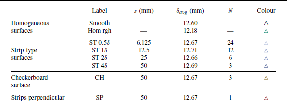


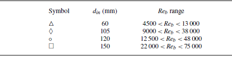


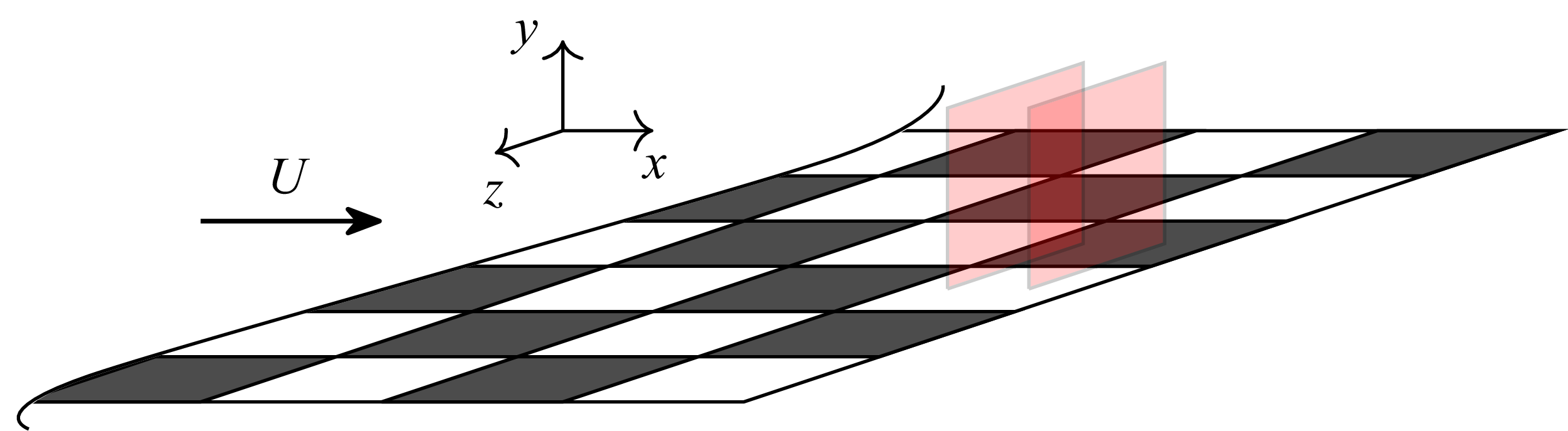


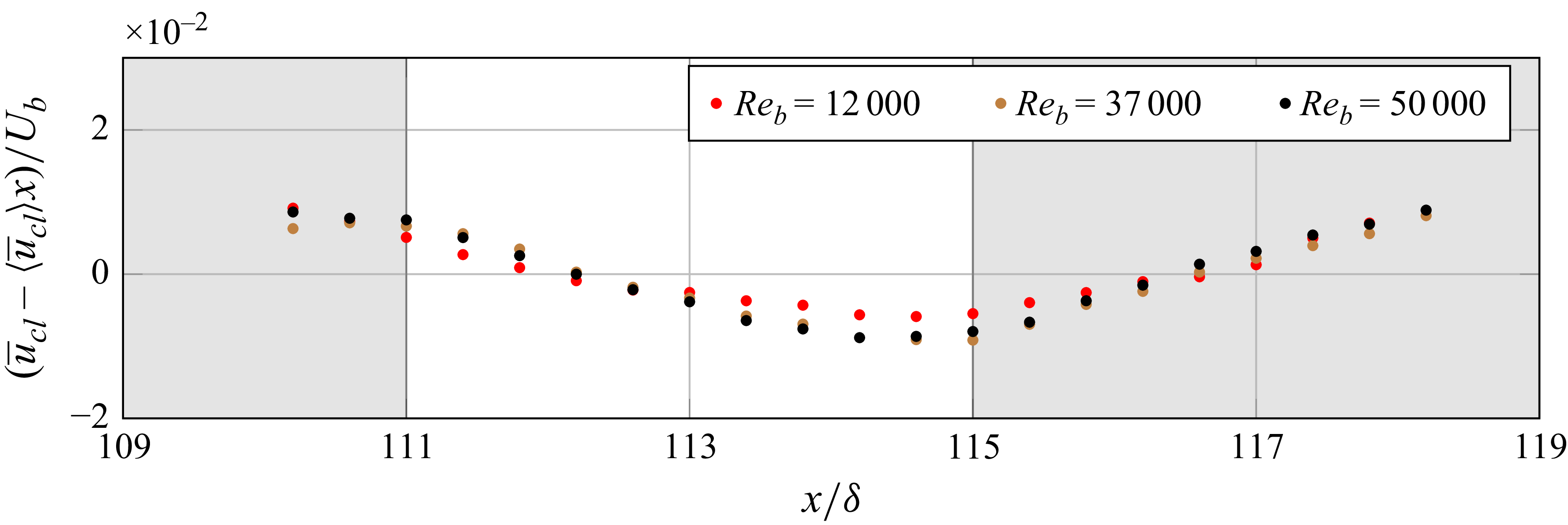

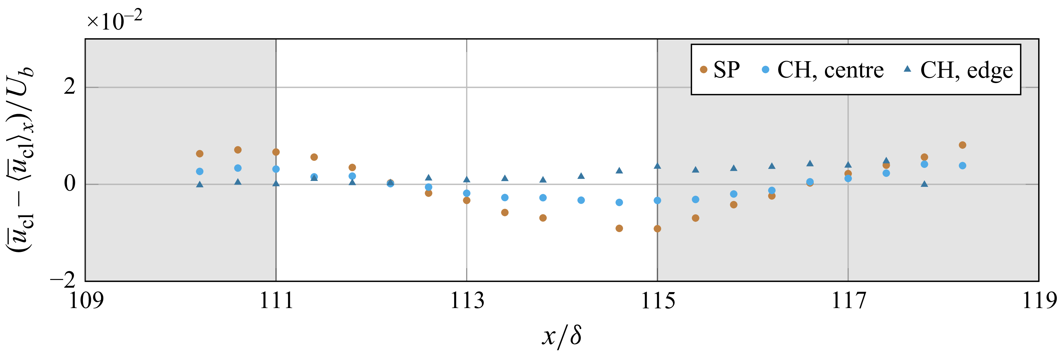


 Open access