Introduction

The ECM technique has been used to identify seasonal snow-accumulation layers in ice cores to great depths (Reference HammerHammer, 1983), and is a valuable interpretative tool in dating complicated ice-sheet chronologies, especially when used in conjunction with measurements made on other physical and chemical parameters of the core (Reference SteffensenSteffensen, 1988; Reference Hammer, Oeschger and LangwayHammer, 1989). Unlike the volcanic-debris index horizons, the seasonality of acid peaks is mainly caused by a combination of seasonal changes in the sources of H₂SO₄ and HNO₃ as exemplified for the Byrd Station core by Reference HammerHammer (1983).

Background

The Byrd Station, West Antarctica (80° S, 120° W), deep ice core (BS68) is 2191 m long and represents the second continuous ice core drilled to bedrock through a polar ice sheet (Camp Century (1966) was the first). The vertical thickness of the ice sheet at Byrd Station is 2164 m. The discrepancy between core length and vertical thickness is accounted for by the 15° inclination measurement at the bottom of the borehole. At bedrock, the interface temperature of the ice is at the pressure-melting point of –1.8°C (Reference Ueda and GarfieldUeda and Garfield, 1969). The drill site is located about 600 km from the coast and 1530 m a.s.1. Today's mean annual surface temperature is –28°C and the area receives about 10 cm w.e. precipitation per year (reported values range from 8 to 12 cm ice a^-1(Reference Gow, de Blander, Crozaz and PicciottoGow and others, 1972)). The low mean annual surface temperature at Byrd Station precludes the existence of summer temperatures above the melting point, Consequently, no disruption of summer snow layers takes place by melting nor has melting occurred during the recorded past. The BS68 core is essentially free of visibly observed melt features or dirt bands, but it did contain locally visibly derived volcanic ash layers from the Executive Range, West Antarctica (Reference Gow and WilliamsonGow and Williamson, 1971). Since it was recovered in 1968, a variety of glaciochemical and climatic studies have been performed on the core (e.g.Reference Johnsen, Dansgaard, Clausen and LangwayJohnsen and others, 1972; Reference Ueda and GarfieldThompson and others, 1975; Reference Cragin, Herron, Langway, Klouda and DunbarCragin and others, 1977; Reference Hammer and GoldbergHammer, 1982; Reference Palais and LegrandPalais and Legrand, 1985; Reference Langway, Osada, Clausen, Hammer, Shoji and MitaniLangway and others, 1988). Although these studies have added greatly to our knowledge of the climatic and paleo-environmental conditions existing during the Wisconsin ice age and the post-glacial Holocene period, most of the published scientific information was derived by performing sequential analyses on non-continuous or on selected depth intervals of the core. This was done because of both practical and technical limitations, e.g. unsatisfactory core quality or continuity or restraints in techniques available at the time.

In contrast to the three Greenland deep ice cores from Camp Century, Dye 3 and Summit, the BS68 core contains a high acid content over the core interval represented by the Wisconsin ice age. In the Arctic regions of the Northern Hemisphere, large amounts of unconsolidated loess and alkaline-earth materials were swept from the continents and exposed continental shelves during low sea levels and neutralized the acid atmospheric aerosol (Reference Cragin, Herron, Langway, Klouda and DunbarCragin and others, 1977; Reference Hammer, Clausen and DansgaardHammer and others, 1980, Reference Hammer, Clausen, Dansgaard, Neftel, Kristinsdottir, Johnson, Langway, Oeschger and Dansgaard1985). A straight-forward detection of seasonal changes in acidity and acid volcanic signals by the electrical ECM method (Reference HammerHammer, 1980) is not possible in Greenland ice cores over the ice-core intervals covering glacial ages, because of their alkaline composition; the ECM can probably be used as a dating tool also for alkaline ice but this interesting possibility is beyond the scope of this paper and requires further studies on alkaline ice. The calibration curve used for the BS68 core was [H+] = 0.045.I^1.73, where H+ is given in μeq. Kg^-1 and the electrical current in μA

In addition, at some Greenland locations, such as Dye 3, an average of almost 6% of the annual accumulation layers consist of summer melt features (Reference Herron, Herron and LangwayHerron and others, 1981), which also complicates the acidity record (Reference Hammer, Clausen, Friedrich and TauberHammer and others, 1987; Reference Clausen and HammerClausen and Hammer, 1988; Reference Clausen, Langway, Oesehger and LangwayClausen and Langway, 1989).

However, in general, strong acids represent an important component of the total chemical constituents found in polar ice and the cores mirror major changes in the past atmospheric content of acidic trace gases such as NO_x, SO_x and HCl. This paper prcsents a stratigraphic daling of the Byrd Station core based on a study of continuous measurement of the atmospheric aeidity-concentration levels inferred by using the ECM technique on the BS68 core remaining at the time of the measurement (1982).

Samples

Certain depth intervals or sections of both the Greenland and Antarctic cores when recovered were highly fractured and broken over an identifiable depth interval, the so-called “brittle zone” (Reference Shoji, Langway, Langway, Oeschger and DansgaardShoji and Langway, 1985). This brittle zone is at least in part caused by clathrate-hydrate formation which takes place at a depth where a combination of high maximum stresses and minimum temperatures exist at their in-situ confining environment. Immediately after drilling, the core undergoes elastic recovery and, at the surface where the core is subjected only to ambient atmospheric pressure, severe fracturing of the core in the “brittle zone” occurs. Also, drilling fluid may seep into the inner part of the fractured ice core within the fractured zone. Removing the outer part of the ice core in this section is not always adequate to eliminate contamination. For this reason, the 300–880 m depth interval of the BS68 core could only be measured for acidity along a few short sample increments; a continuous acid-volcanic record is not available here. When the Dye 3 deep-ice core (D3/81) was drilled during the GISP 1979–81 operation (Reference DansgaardDansgaard and others, 1982) and the GRIP drilling at Summit 1989-92 (Reference Langway, Clausen and HammerJohnsen and others, 1992), the occurrence of the brittle zone was anticipated and proper preparations led to a complete and satisfactory field measurement of acidity and the anions.

The BS68 core was drilled about 24 years ago and the acidity measurements for this study were made about 14 years later. As a consequence, the physical quality of the core had somewhat deteriorated due to stress relaxation and the slight temperature variations which occurred during its long transportation and storage (Reference Shoji, Langway, Langway, Oeschger and DansgaardShoji and Langway, 1985). This was also the case for the Camp Century, Greenland, deep-ice core (CC66), which was analyzed for acidity and reported earlier (Reference Hammer, Clausen and DansgaardHammer and others, 1980). On a comparative basis, the BS68 core was originally recovered in a much better physical and continuous condition, and the acidity profile was made using a much-improved measuring technique than was the case for the (CC66) core study; except for the brittle zone, it was sufficient to remove only 1–2 cm from the outer part of the BS68 core to obtain reliable and reproducible ECM measurements.

Procedures

The entire BS68 core was measured by the ECM at –23°C (the temperature in the cold-storage warehouse in Buffalo), except for about 50m of selected ice-core sequences, which were also measured at both -30° and –12”C in the SUNY at the Buffalo Ice Core Laboratory. The laboratory measurements were made in order to estimate the activation energy E_a for the electrical conduction process. The calculated E_a was 0.23 eV. This value was used to calculate the current corresponding to -14°C, which was the temperature of the ice cores used for establishing the calibration curve. The acidity of the BS68 core was measured using the electrical d.c. conductivity method (now commonly called ECM), which is essentially a measure of the electrical current (Reference HammerHammer, 1980). In principle, the ECM infers the acidity-concentration level in the ice core, whereas pH refers to measurements made on melted samples. The difference is usually of little importance in interpreting Holocene ice deposits hut, due to chemical reactions in the liquid state, the two acidity estimates may differ, especially when large amount of impurities are present. The latter case was of particular concern in the (CC66) study, as the late Wisconsin ice-core samples were found to contain up to two orders of magnitude higher impurity content and particle concentrations than did the Holocene ice (Reference Hammer, Clausen, Dansgaard, Neftel, Kristinsdottir, Johnson, Langway, Oeschger and DansgaardHammer and others, 1985). Conversely, the ECM measurements made over the glacial ice in the BS68 core, which has a much lower dust concentration, were found to follow the empirical (H+) calibration curve of Reference HammerHammer (1980). The calibration curve has later been found to vary somewhat from one drill site to another but no specific explanation has yet been found.

The ECM measurements made over the 50 000 year chronology provided more than 1.6 × 10₆ data points with a resolution of a few millimeters. Liquid-acidity (pH) and anion-concentration levels of important core sequences were measured and analyzed by pH and ion chromatography in both Buffalo and Copenhagen.

Dating the core

The commonly low annual snow accumulation in Antarctica makes it difficult to use independently the δ ¹⁸O method to determine accurately seasonal changes (Reference Johnsen, Dansgaard, Clausen and LangwayJohnsen and others, 1972; Reference Dansgaard, Johnsen, Clausen and GundestrupDansgaard and others, 1973). Various other indirect dating methods have been used in the past to date the BS68 core (Reference Johnsen, Dansgaard, Clausen and Langwayjohnsen and others, 1972; Reference Thompson, Hamilton and BullThompson and others, 1975; Reference Lorius, Merlivat, Duval, Jouzel, Pourchet and AllisonLorius and others, 1981) but no acceptable systematic method previously existed for continuous stratigraphic dating the early Holocene and late Wisconsin of the ice core.

The top almost 88 m of the icE core from BS68 was recovered in an unsatisfactory physical condition which precluded using it for detailed laboratory analyses. In order to establish a proper reference horizon for our time-scale, we first determined two fixed horizons; the AD 1968 snow surface and the AD 1259 volcanic—chemistry stratigraphic event (Reference Langway, Osada, Clausen, Hammer, Shoji and MitaniLangway and others, 1988). The AD 1259 layer lies 97.8 m below the AD 1968 surface reference.

Using the depth-density data for this core interval, we obtained an average annual accumulation-layer thickness, λ, of 11.2 cm of ice equivalent for the 709 years represented. A recent integrated study (Reference JohnsenLangway and others, 1994) on a new 164 m deep ice core recovered at Byrd Station in 1989 (NBY-89) provides us with a detailed up-to-date and continuous annual-layer stratigraphic chronology for the last 1360 years (1989-AD 629). An average ice-layer thickness, λ, of 11 cm of ice equivalent is given for this 1360 year time interval. The NBY-89 core time-scale and chemistry-stratigraphy also connect with the earlier BS68 core records at several volcanic and chemical index horizons, including the prominent AD 1259 event. These results substantiate our upper profile time-scale and further establish the AD 1259 event as a fixed, pronounced and reliable inter-hemispheric reference level for the new results presented here.

Fig. 1.

The acidity measurements ( ECM ) in µeq. H₊ kg_-l on the Byrd Station deep core (BS68). Figure 1a and b are representative curves of Holocene ice from above the “brittle zone”. Figure 1c and d are from Holocene ice below the “brittle zone”. Figure 1e is from the Holocene Wisconsin (H.W ) transition in the ice core. Figure 1f–h represent ice .From the Wisconsin glaciation. The ECM-resolution curves are plotted on averaged 1 cm intervals for Figure la-c, with a resolution of 0.5 cm for Figure ld–f and with 0.2 cm for Figure 1g-h. Each core section is 1.20 m in length but for Figure 1h a shorter section is shown. The curves show multiple-year annual acid layers (λs). Note the decreasing value of λs with depth.

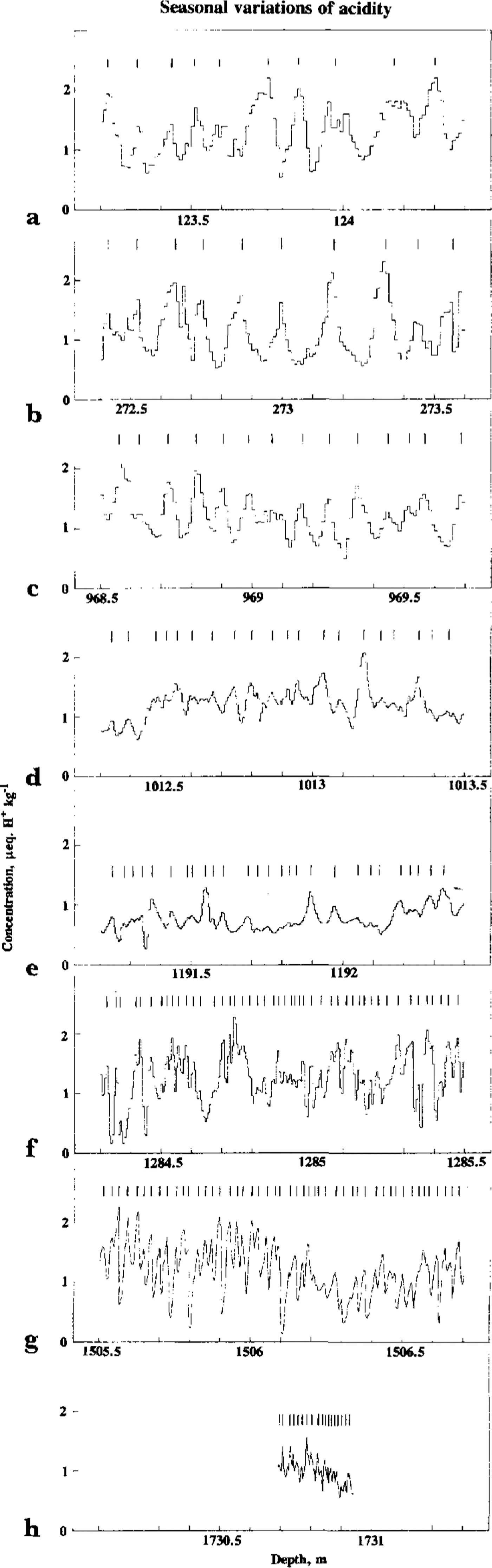
Figure 1shows examples of the acid seasonal variations at several representative depths in the BS68 core. Systematic annual curves are very clear for all depth levels down to about 1600 m. Below this depth, the seasonal signal becomes more complicated. This change is most probably related to the large increase in crystal size which begins here as a result of higher in-situ temperatures (Reference Gow, Ueda and GarfieldGow and others, 1968) brought about by the geothermal heat flux and deformation. The systematic chronological record for the lower part of the core has been disturbed by non-laminar glacier flow over the rugged bedrock topography; the lowest 9 m of high-silt content basal ice, which is not included in our study, is probably much older than the immediate overlying ice; the high values (Reference Johnsen, Dansgaard, Clausen and LangwayJohnsen and others, 1972) suggest that Eemian ice is present.

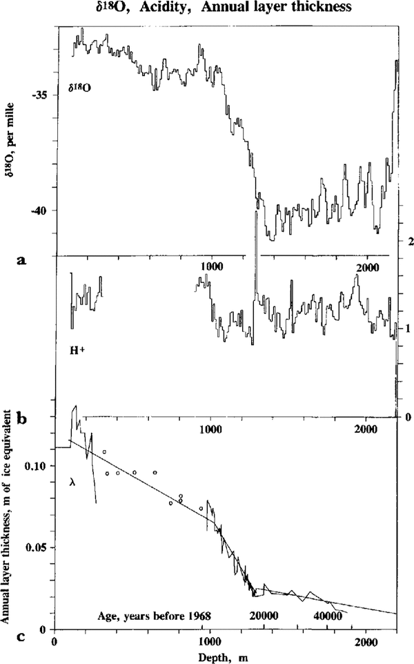
Figure 2shows the δ ¹⁸O curve (Fig. 2.), the ECM curve (Fig. 2.) and the interpreted annual ice-layer thickness (λ) curve (Fig. 2.) for the core. Because of the missing λ data in the brittle zone, our dating of the Byrd Station core was accomplished by an averaging process instead of using the actual λ versus depth relationship. The three straight-line segments in Figure 2 represent hinge points where major changes in average λs occur. The lines are based on the individual λs over the respective depth intervals. As shown, the λs decrease significantly but systematically with depth. The slope of the curve from near the surface downward shows a gradual decrease due mainly to deformation until a sharper decrease occurs at about 1000 m. The curve tends to flatten out to a lower rate of decrease at about 1300 m down to about 1910m. The curve has been extended to the bedrock. as we have indications of seasonal variations down to around 2150 m. The extended λ curve does not intersect the origin at the bottom of the curve, probably because active melting occurs here and a value different from zero is to be expected. The slope of the curve between 18 and 50ka BP (1294 1910m) suggests that an average annual precipitation rate of about 5 cm of ice equivalent occurred at the surface during the late to mid Wisconsin (based on flow-dynamics considerations). The annual seasonal variations in acidity are observed down to about 1750 m, corresponding to 40 000 years BP. Between 1750 and 1910 m, the λs are still present but arc more difficult to resolve. We believe that our dating of the ice-core record is valid and continuous to 1910 m,corresponding to 50 000 years BP. Any dating below 19l0 m is probably less accurate.

Fig. 2.

Theδ ¹⁸O and ECM acidity-concentration values plotted as 10 m averages vs depth and the λs for the BS68 core. Figure 2a shows the δ ¹⁸O values in ppt and Figure 2b shows the ECM acidity levels. An omission exists in the curve for Figure 2b between the surface and about 90 m (see text) and between 300 and 890m (brittle zone). Figure 2c shows the average annual ice-layer thickness curve (λ). A few sequences could be used for detection of s in the brittle zone (circles) but not for absolute values of acidity.

There is, of course, a certain amount of subjectivity in identifying annual layers, e.g. in Figure 1, but the ECM “seasonals” can be followed continuously along the core and the corresponding “λs” decrease with depth are as expected from flow-dynamical considerations, assuming a constant accumulation down to about 1000 m.

The correctness and accuracy of the dating for the first 100 m are indicated by the integrated study of the NBY89 and BS68 cores. Sequentia1 IC chemical analysis clearly demonstrates that the seasonality of the ECM is almost entirely due to a strong seasonal cycle of H2S04 and to a lesser extent to HNO₃. The sulphate and nitrate actually seem to peak during the warm half-year of the Southern Hemisphere. Whilst there is some evidence for the ocean around West Antarctica as a source area for the seasonally varying sulphuric acid (Reference Prospero, Savoie, Saltzman and LarsenProspero and others, 1991), the seasonal variation of the nitrate concentration is a more complex phenomenon to explain. This pronounced seasonality of nitrate is also clearly seen in Greenland ice cores (Reference SteffensenSteffensen, 1988).

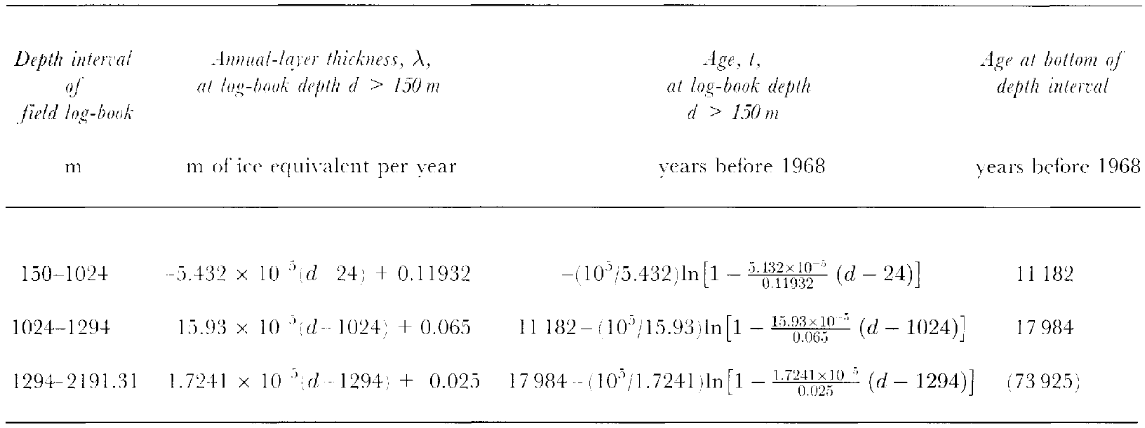
However, since nitrate and dust concentrations can be measured continuously and with high resolution along an ice cure, we recently measured an increment of glacial ice from the BS68 core around 1285 m to check our annual-layer interpretation of the gIacial ECM profile. The measurements showed that all three profiles indicate the same “average annual-layer thickness” over the core increment (to be published elsewhere). Still, there is a certain amount of subjectivity in the interpretation of the annual cycles of both ECM, dust and nitrate, Which suggest that our dating precision of a 20 000 year old ice layer is probably ±1000 years. Using the three straight-line approximations shown in Figure 2, it is possible to express the age- depth relationship of the BS68 core in the mathematical equations given in Table I. The accuracy of the time-scale at the 11 000 year BP level is approximately ± 500 years; the high uncertainty is due mainly to the brittle zone.

Theδ, ecm and λ profiles

Figure 2 shows δ ¹⁸O plotted for the entire BS68 core as 10 m averages. The 10 m averages depict a greater number of years as one descends in depth. The δ ¹⁸ like λs are climatic parameters, which on average gradually decrease from the Holocene to the Wisconsin: they rapidly decrease during the Holocene/Wisconsin transition and fluctuate considerably but at lower (colder) levels in the Wisconsin ice age than in the Holocene period. There is, however, no clear indication that the shift in the δ ¹⁸O values observed around 1080 m (corresponding to 12.1 ka BP on our scale) coincides with the sharp decrease shown in λs (Figure 2). The dip in the s at 1005 m corresponds to an age of 10.9 ka BP. In other words, the δ ¹⁸O curve does not show an easily identified junction between the Holocene and the Holocene-Wisconsin transitional zone. Note the ± ±2-3‰ change of δ ¹⁸O during the Holocene; this may partly be explained by upstream ice-flow conditions during the Holocene, which must be scrutinized before the Byrd Station and Arctic ice-core δ record can be compared in a more detailed way. Details and discussion of the entire δ ¹⁸O have already been published (Reference Johnsen, Dansgaard, Clausen and LangwayJohnsen and others. 1972). The Holocene– Wisconsin transition is identified as being approximately between 1080m (12.1 ka BP and 1294 m (18.0 ka BP), a 214 m core interval which represents about 5900 years.

Figure 2 shows a plot of the 10 m average acidity values in μeq. H+kg^-1. The interval between 90 and 990 m shows higher average acid values than those measured in the Holocene—Wisconsin transition and the Wisconsin age (between 18 and 50 ka BP), although the Wisconsin ice has a relatively higher average-acidity level than the Holocene–Wisconsin transition. The off-scale acidity value between 1280 and 1290 m (2.3μeq. H+ kg^-1 ) is by far the single highest acidity value in the entire core (the event is due to excessive volcanism and will be published in detail elsewhere).

The decrease in λs from the present day (11.2 cm of ice equivalent) to the end of the Holocene-Wisconsin transition, (6.5cm of ice equivalent) is the result of thinning of beds load compaction and stretching of layers) The average accumulation during the Holocene including the brittle zone is approximately 11.9cm of ice equivalent. During the Holocene Wisconsin transition, the λs decrease in a step-like manner from about 6.5cm at 1024m to about 2.5 cm just below 1294m and. finally, to about 1.5 cm at 1910 m.

Discussion of the time-scale

This study strongly indicates that seasonal periodicity of the background-level acid concentrations clearly persists over the BS68 core measured between 88 and 1910 m depths. Below this depth, annual acid layers arc difficult to assess. Results of annual-layer-thickness analysis from the ECM measurements include the effect of thinning of beds due to flow deformation and the effect of climatic change as depicted in the δ ¹⁸O curve. Based on the arguments presented above. it seems evident that the ECM profile has a strong seasonal character but other arguments, which substantiate this finding, can be brought into the discussion.

The reported low concentration levels of impurities in the core (Reference Thompson, Hamilton and BullThompson and others, 1975: Reference Hammer and GoldbergHammer, 1982; Reference Palais and LegrandPalais and Legrand. 1985; Reference Langway, Osada, Clausen, Hammer, Shoji and MitaniLangway and others, 1988) rule out an impurity influence on the flow law as an explanation of the λ changes during the Holocene-Wisconsin transition. This explanation is confirmed by recent borehole measurements (Reference Hansen, Kelty and GundestrupHansen and others, 1989). It appears that the annual precipitation in the Byrd Station area, and probably over the entire West Antarctic ice sheet in general, increased about 2.5 times during the transition from the Late-Glacial ice age to Holocene times. Similar changes in λs have been observed in the Greenland deep-ice cores (Reference Hammer, Clausen and TauberHammer and others, 1986: Reference Langway, Clausen and HammerJohnsen and others, 1992), though the data for the Dye 3 and Camp Century cores arc sparse

Recent statistical studies of annual λ/δ ratios at various Greenland sites over the past 200 years (Reference Clausen, Gundestrup, Johnsen, Bindsehadlcr and ZwallyClausen and others, 1988) show about an 8% change in thc accumulation rate for each per mille change in δ ¹⁸O. This ratio is also derived from a precipitation model (Reference Johnsen, Dansgaard and WhiteJohnsen and others, 1989: personal communication from S. Johnsen). If this relation is applied to the approximately 7.5‰δ ¹⁸O change over the transition found in thc Byrd Station core, (Fig. 2a), one would expect a change in the annual precipitation by a factor of 2.5.

Our results also indicate that a significant part of the enhanced ₁₀Be concentrations found in ice cores over glacial times (Reference Raisbeck, Yiou, Bourlcs, Lorius, Jouzel and BarkovRaisbeck and others, 1987; Reference BeerBeer and others, 1988) mainly reflect a lower rate of precipitation rather than increased ¹⁰Be production in the atmosphere. The ^lOBe concentration peaks observed in the Antarctic Dome C and Vostok ice cores, and the Greenland Camp Century core, probably have other explanations, and require further study to establish their bi-hemispheric significance as global reference horizons. ^lOBe measurements on the new Summit deep-ice core from Greenland should be able to solve this problem.

The dip in the BS68 δ ¹⁸O curve around 12.1 ka BP ± 0.5 ka could correspond to the Younger Dryas -Pre-Boreal (YD–PB) time interval in the new Greenland Summit ice cores. The sharp YD-PB transition in the Greenland cores (D3/81, CC66) has been dated as 10.750 ka BP ± 0.15 ka (Hammer and others, 1986) but, based on new data from Greenland, we obtained a value of 11.5 ka BP ± 0.1ka (Reference Langway, Clausen and HammerJohnsen and others, 1992) and 11.6ka BP ± 0.3 ka (Reference AlleyAlley and others, 1993). 1t is also interesting to note that the BS68 annual-layer-thickness curve (Figure 2) shows a dip around 1024m; this depth corresponds to 11.2 ka BP in our Byrd Station time-scale and could also correspond to the YD-PB boreal transition in Greenland ice cores. However, the dating accuracy of the BS68 core does not allow a confident comparison between the “details” of the δ ¹⁸O curve of the BS68 core and the corresponding Greenland records; the same applies to the East Antarctic deep ice cores from Vostok and Dome C (Reference Lorius, Merlivat, Jouzel and PourehetLorius and others, 1979, Reference Lorius1985). Such a comparison would have to await new well-planned deep drilling in Antarctica.

Table 1.

Depth age relationship. Calculated annual-layer thicknesses, λ, and ages, t, given. field log-book depths, d > 150 m. based on the linear decreasing values of the λ _s by depth over the three depth intervals, shown in Figure 2c. The slope of the lines, α. are –5.432 × 10⁵a¹, -15.93 × 10⁵ a ¹ and –1.7241 × 10^-5a ^-1, respectively Those slopes are determined by hinge points in the intervals. For the top 1000 m of ice equivalent (the subtracted 24 m corresponds to the amount of air in the upper 150 m of firn layers), the hinge points are 0.11932 and 0.065 m of ice eq. a¹ . For the next 270 m, the hinge points arc 0.065 and 0.222 m of ice eq. a1 and for 870 m of the last interval 0.025 and 0.010 m of ice eq. a¹. Thus, the age. T1, al any depth, d1 > 150m, in the top interval, is determined bv t1 =(1/α1) × ln [ l + (α1/0.11932) × (d1-24)]

Acknowledgements

The initial pilot study of the ECM investigation reported here was made in 1980 and the complete measuring programme was conducted in 1982 in the commercial ice-core-storage warehouse in Buffalo, New York. All of the original 2088 core tubes existing at that time were individually opened and the core remaining in the tubes was measured in the cold room over a 2½ month period. The authors regret the delay in publishing the full results but inadvertent postponements were experienced by new and often unrelated field and laboratory research obligations and divergent schedules. Some laboratory assistance for a variety of ionic chemistry measurements was made by K. Osada at the SUNYIBuffalo Ice Core Laboratory. We are indebted to the Danish Natural Science Research Council (SNF), the Commission for Scientific Research in Greenland (KVCG) and the U.S. National Science Foundation (NSF/DPP) for support covering various periods of the study.