





1. Introduction
Shock wave/turbulent boundary layer interactions (SBLIs) are a typical hallmark of high-speed aerodynamics. Common examples of SBLIs can be found both in external flows, such as transonic/supersonic airfoils, wing–body junctions and aircraft control surfaces, and in internal flows, such as engine supersonic inlets (Smits & Dussauge Reference Smits and Dussauge2006). Shock impingement on boundary layers often results in extensive reversed flow, with associated low-frequency unsteady pressure loads mainly localized near the separation line as a result of motion of the reflected shock foot. Low-frequency pressure fluctuations pose serious concerns to aircraft design, as they are prone to trigger fluid–structure interaction phenomena with potential structural damage. As a result, this phenomenon has been extensively studied, and is reviewed in several reference papers (Dolling Reference Dolling2001; Clemens & Narayanaswamy Reference Clemens and Narayanaswamy2014; Gaitonde & Adler Reference Gaitonde and Adler2023).
Most experimental and numerical studies are generally focused on ‘two-dimensional’ configurations, in which the shock impingement line is orthogonal to the incoming flow. In this canonical set-up, the general consensus is that two main driving mechanisms are responsible for low-frequency unsteadiness (Clemens & Narayanaswamy Reference Clemens and Narayanaswamy2014). For mildly separated flow, unsteadiness is mainly linked to advection of large-scale structures embedded in the incoming boundary layer (‘upstream mechanism’; see e.g. Ganapathisubramani, Clemens & Dolling (Reference Ganapathisubramani, Clemens and Dolling2009) and Humble et al. (Reference Humble, Elsinga, Scarano and Van Oudheusden2009)). For strongly separated flows, periodic expansion and contraction resulting in ‘breathing’ of the separation bubble is believed to play a major role (‘downstream mechanism’; see e.g. Piponniau et al. (Reference Piponniau, Dussauge, Debiève and Dupont2009) and Touber & Sandham (Reference Touber and Sandham2009)). In practice, the upstream and the downstream mechanisms coexist, their relative importance depending on the strength of the impinging shock (Souverein et al. Reference Souverein, Dupont, Debiève, Dussauge, van Oudheusden and Scarano2009).
A scaling law for low-frequency pressure oscillations in strong interactions was inferred by Dussauge, Dupont & Debiève (Reference Dussauge, Dupont and Debiève2006) based on analysis of existing SBLI data. Specifically, they showed that the typical frequencies scale with the size of the separation bubble (say,  $L_{{sep}}$) and with the upstream velocity ( $u_0$), resulting in typical Strouhal numbers $St_{L} = f L_{{sep}}/u_0 \approx 0.03\unicode{x2013}0.05$. This scaling was later explained by Piponniau et al. (Reference Piponniau, Dussauge, Debiève and Dupont2009) as resulting from breathing motion of the separation bubble and associated shear layer flapping along the bubble upper boundary. A possible physical explanation for breathing motion of the separation bubble has recently been offered by Sasaki et al. (Reference Sasaki, Barros, Cavalieri and Larchevêque2021), who found that the only causal inputs that are highly correlated with shock motions reside around and downstream of the recirculation bubble, and envisaged the occurrence of an acoustic feedback loop mechanism as originally argued by Pirozzoli & Grasso (Reference Pirozzoli and Grasso2006).
In practical applications, the shock impingement line is, however, seldom orthogonal to the incoming boundary layer. Depending on the shock strength and the sweep angle, the interaction is characterized by either parallel or diverging separation/reattachment lines along the spanwise direction, which correspond to cylindrical or conical symmetry conditions, respectively (Settles, Perkins & Bogdonoff Reference Settles, Perkins and Bogdonoff1980). This is the case for flows over swept compression ramps (Settles et al. Reference Settles, Perkins and Bogdonoff1980; Erengil & Dolling Reference Erengil and Dolling1993; Vanstone et al. Reference Vanstone, Saleem, Seckin and Clemens2017; Adler & Gaitonde Reference Adler and Gaitonde2018, Reference Adler and Gaitonde2020), around sharp fins (Schmisseur & Dolling Reference Schmisseur and Dolling1994; Gaitonde et al. Reference Gaitonde, Shang, Garrison, Zheltovodov and Maksimov1999; Arora, Mears & Alvi Reference Arora, Mears and Alvi2019) and for swept impinging oblique SBLIs (Doehrmann et al. Reference Doehrmann, Padmanabhan, Threadgill and Little2018; Padmanabhan et al. Reference Padmanabhan, Maldonado, Threadgill and Little2021). All the above studies of swept SBLIs agree about the importance of three-dimensional effects on low-frequency unsteadiness, with consensus on an increase of the typical frequencies with the sweep angle.
However, whereas early experimental studies (Erengil & Dolling Reference Erengil and Dolling1993) suggested a continuously increasing trend with the sweep angle, recent numerical studies (Adler & Gaitonde Reference Adler and Gaitonde2020) rather seem to indicate suppression of the low-frequency peak in the presence of three-dimensional effects, on account of a topological change of the separation bubble from a closed to an open type. Another important issue in swept interactions is the possible variation of the typical frequencies along the spanwise direction. Whereas Erengil & Dolling (Reference Erengil and Dolling1993) suggested a spanwise decrease of the typical frequencies, more recent studies tend to support invariance (Adler & Gaitonde Reference Adler and Gaitonde2020; Padmanabhan et al. Reference Padmanabhan, Maldonado, Threadgill and Little2021).
Given this background and the importance of the subject, we believe that a deeper understanding of the physical mechanisms underlying low-frequency unsteadiness in swept SBLIs is appropriate. For that purpose, we leverage a novel direct numerical simulations (DNS) dataset based on the idealized set-up originally considered by Gross & Fasel (Reference Gross and Fasel2016) in which both the shock strength and the flow sweep angle are varied. Proper orthogonal decomposition (POD) and frequency–wavenumber spectra of the wall pressure distribution are then used to infer the characteristic length and velocity scales of the problem, based on which a scaling law for the typical frequencies of pressure fluctuations is derived.
2. Computational set-up
The flow set-up replicates that used in previous studies aimed at establishing the effects of cross-flow on SBLIs (Gross & Fasel Reference Gross and Fasel2016; Lee & Gross Reference Lee and Gross2021; Di Renzo et al. Reference Di Renzo, Oberoi, Larsson and Pirozzoli2022; Larsson et al. Reference Larsson, Kumar, Oberoi, Di Renzo and Pirozzoli2022), as sketched in figure 1. The boundary layer is injected through the inflow plane  $x=0$ with sweep angle $\gamma _0$, and an oblique shock wave ( $\beta$ is the shock angle) is introduced by deflecting the flow by an angle $\theta$, which nominally impinges on the boundary layer at $x_{{imp}} = 64 \delta _0$. The $x$-projected Mach number is kept constant at $M_{0,x} = u_{0,x}/c_0=2.28$, where $u_{0,x} = u_0 \cos \gamma _0$ is the $x$-projected free-stream velocity and $c_0$ is the free-stream sound speed, resulting in varying free-stream absolute Mach number $M_0 = M_{0,x}/\cos \gamma _0$. Several values of $\gamma _0$ and $\theta$ have been considered, as listed in table 1. The spanwise size of the computational box ( $L_z$) is varied from $8\delta _0$ (similar to most previous studies, and labelled as NRW) to $96\delta _0$ (much wider than in any previous studies). It turns out that this choice has substantial impact, as discussed next. A mesh with $N_x \times N_y \times N_z = 1920 \times 240 \times 2016$ nodes is used for DNS in large boxes, whereas $N_z=168$ is used for the NRW cases. The streamwise and wall-normal domain sizes are set to $(L_x \times L_y)/\delta _0 = 96 \times 20$ for all cases.
Numerical set-up for swept SBLI analysis. Here  $\delta _0$ is the inflow boundary layer thickness, $\gamma _0$ is the inflow sweep angle, $x_{{imp}}$ is the nominal shock impingement position, $\beta$ is the shock inclination angle and $\theta$ is the flow deflection angle.

Flow parameters for the DNS database:  $M_0$ is the free-stream Mach number, ${M_{0x}}$ is its $x$ projection, $\gamma _0$ is the incoming flow sweep angle, $\theta$ is the flow deflection angle, $Re_{\delta _0} = \rho _0 u_0\delta _0/\mu _0$ is the inflow Reynolds number, $L_x,L_y,L_z$ is the size of the computational box, $L_{{sep}}$ is the separation bubble extent, and $St_{L,{pk}}$ and $St_{L,{min}}$ are the peak and the minimum resolved Strouhal numbers and $T$ is the time window used for the spectral analysis. The suffix NRW refers to DNS carried out in narrow domains ( $L_z=8 \delta _0$).

An in-house solver, available as an open-source code (Bernardini et al. Reference Bernardini, Modesti, Salvadore and Pirozzoli2021), is used for all the DNS. Numerical boundary conditions at the far-field boundaries are managed according to a characteristic relaxation strategy (Pirozzoli & Colonius Reference Pirozzoli and Colonius2013). The recycling–rescaling procedure is used to generate the target flow at the inflow, as described by Ceci et al. (Reference Ceci, Palumbo, Larsson and Pirozzoli2022). The impinging shock is generated through local enforcement of the Rankine–Hugoniot jump relations at the top boundary, and periodic boundary conditions are applied to the spanwise boundaries. The wall is assumed to be isothermal, with temperature set to the nominal adiabatic value.
Averaging is started after statistically steady conditions are established, as estimated by monitoring the time history of the spanwise-averaged separation point. The minimum resolved Strouhal numbers ( ${\textit{St}}_{{min}} = L_{sep}/(u_{0,x}T)$, where T is the time window for the statistical analysis) are reported in table 1. The time window may seem marginal for some of the flow cases, especially the G45_T10 case, in which it would correspond to slightly less than three fundamental cycles if the typical Strouhal number was $St \approx 0.03$. However, one of the key results of the present study – see figure 8(a) and related discussion – is that the peak Strouhal number (also reported in table 1) increases significantly with the skew angle, hence the effective number of resolved low-frequency cycles is much higher. The spectra hereafter reported have been obtained by sampling the data at time intervals $\Delta t = 0.27 \delta _0/u_{0,x}$, and using the Welch method by splitting the signal into eight segments with 50 % overlap, upon use of Hamming windowing. The same samples are used also for the POD analysis, which we carry out following Sirovich (Reference Sirovich1987).
3. Analysis
The effect of the spanwise width on some basic flow properties (namely, friction coefficient and wall pressure variance) is addressed in figure 2. As shown in previous studies (Di Renzo et al. Reference Di Renzo, Oberoi, Larsson and Pirozzoli2022; Larsson et al. Reference Larsson, Kumar, Oberoi, Di Renzo and Pirozzoli2022), the presence of a non-zero sweep angle yields substantial enlargement of the interaction zone, as compared to the case of two-dimensional, non-swept interactions. However, the effect of the domain width is very limited, in both cases. Maps of the power spectral density (PSD) of wall pressure are shown in figure 3, normalized by the respective variances ( $\hat {E}(f)$), in pre-multiplied form. Consistent with the general wisdom, the non-swept case shows the occurrence of low-frequency dynamics at $10^{-2} \lesssim St_L \lesssim 10^{-1}$, in a limited space interval around the mean separation point. No obvious effect of the spanwise domain size is visible in that case, although, of course, the spectra collected in the wider domains are smoother as a result of averaging in the spanwise direction. The swept case in small domains (figure 3c) also shows a similar pattern, on account of previously noted differences in the size of the interaction zone. Quite surprisingly, DNS of the swept case in a large domain (figure 3d) shows substantial increase of the peak frequency, which was the original motivation for further analysis.
Distributions of  $x$-projected friction coefficient (a) and wall pressure variance (b). Solid lines denote DNS in the widest domain ( $L_z=96 \delta _0$), and dashed lines denote DNS in the narrowest domain ( $L_z = 8 \delta _0$). In both cases the deviation angle is $\theta =10.4^\circ$. Two-dimensional cases ( $\gamma _0=0^\circ$) are coloured in red, and swept cases (with $\gamma _0=30^\circ$) are coloured in black. The streamwise coordinate is scaled by the boundary layer thickness $\delta _r$ upstream of the mean separation line.

Pre-multiplied normalized PSD of wall pressure for flow cases G00_Lz08 (a), G00_Lz96 (b), G30_Lz08 (c) and G30_Lz96 (d). In all cases  $\theta =10.4^\circ$. The red/purple line denotes the mean separation location, the green line the nominal shock impingement location, and the cyan line the mean reattachment location. Red crosses mark the position of the low-frequency peaks near the separation line. Spectra are also averaged in the spanwise direction.

After discarding possible effects related to spurious flow periodicity along the spanwise direction, which are discussed in Larsson et al. (Reference Larsson, Kumar, Oberoi, Di Renzo and Pirozzoli2022), we turned to analyse the spatial pattern of the wall pressure through POD. Figure 4 depicts the shape of the most energetic POD modes for  $\gamma _0=30^\circ$, in small and large domains, along with their associated PSD. The leading POD mode in the small domain features a spanwise-invariant distribution, with a sharp peak at the mean separation line, and a flatter distribution with opposite sign at reattachment, hence overall reminiscent of bubble breathing. The PSD of the associated temporal coefficient in fact has a peak at $St_L \approx 0.07\unicode{x2013}0.08$, which is very close to the peak value of the pressure PSD in figure 3(c). The leading POD mode in the $L_z = 96 \delta _0$ box is instead characterized by apparent spanwise corrugation around the mean separation line, and by oblique structures stretching up to the reattachment line. The PSD of the associated temporal coefficient peaks at $St_L \approx 0.21\unicode{x2013}0.22$, which is very close to the peak frequency of the temporal PSD at the separation line in figure 3(d). Similar conclusions apply to all cases under scrutiny, including non-swept ones. We find that rippling of the separation line is visible only if sufficiently wide boxes are used, as we have checked with DNS in domains with intermediate size $L_z = \{24,32,64\} \delta _0$, not shown here.
Shape of leading POD mode of wall pressure (a,c) and pre-multiplied normalized PSD of the corresponding temporal coefficient (b,d): (a,b) G30_T10_NRW ( $\gamma _0=30^{\circ}$, $L_z = 8 \delta _0$); and (c,d) G30_T10 ( $\gamma _0=30^{\circ}$, $L_z = 96 \delta _0$). The dashed lines are as in figure 3. In all cases, $\theta =10.4^{\circ}$.

In order to quantitatively characterize the observed rippling of the separation line, in figure 5 we show the PSD of the wall pressure as a function of the spanwise wavelength, scaled either by the incoming boundary layer thickness or by the length of the separation bubble. We argue that marginally better collapse of the PSD across the  $\gamma _0$ range is achieved in the latter case, especially for the extreme $\gamma _0 = 45^{\circ }$ case, which exhibits massive flow separation, and for which even the largest box used here may be barely sufficient. Two spectral peaks are observed, one at small wavelength ( $\lambda _z \approx 0.1 L_{{sep}}$), which would probably correspond to the small-scale rippling noticed in previous numerical simulations of non-swept SBLIs (Pasquariello, Hickel & Adams Reference Pasquariello, Hickel and Adams2017). However, the most prominent peak is found to reside at much longer wavelengths ( $\lambda _z \approx 2 L_{{sep}}$), which cannot be resolved in numerical simulations in small boxes.
Spanwise pre-multiplied normalized PSD of wall pressure at the mean separation line for various sweep angles  $\gamma _0$ at fixed shock strength ( $\theta =10.4^\circ$). The spanwise wavelength $\lambda _z$ is scaled with either (a) the reference boundary layer thickness $\delta _r$ or (b) the separation length. Here $\kappa _z=2 {\rm \pi}/\lambda _z$ is the spanwise wavenumber. The dashed line in panel (b) marks $\lambda _z = 2 L_{{sep}}$.

Wavenumber–frequency spectra at the mean separation line are further considered in figure 6 to characterize the advection velocity of pressure disturbances. Whereas no clear organization is observed in non-swept SBLIs (figure 6a), distinct clustering of the PSD around a linear distribution is found in swept interactions, which becomes more evident at high sweep angles, and which is a clear indication of the presence of convecting disturbances. In particular, data fitting yields  $\omega = w_c \kappa _z$, with convection velocity proportional to the cross-flow free-stream velocity, namely $w_c \approx 0.7 u_{0,z} = 0.7 u_{0,x} \tan \gamma _0$.
Contour plots of spanwise wavenumber–frequency spectra of wall pressure at the mean separation location. Dashed lines denote the linear relationship  $\omega = \kappa _z w_c$, with convection velocity $w_c = 0.7 u_{0,x}\tan {\gamma _0}$: (a) $\gamma _0 = 0^\circ$; (b) $\gamma _0 = 15^\circ$; (c) $\gamma _0 = 30^\circ$; and (d) $\gamma _0 = 45^\circ$. In all cases $\theta =10.4^\circ$. The blue crosses mark the position of the low-frequency peaks.

4. Model synthesis
Based on the above evidence, we are led to formulate a tentative model for the behaviour of pressure fluctuations near the separation line in swept SBLIs, as sketched in figure 7. Specifically, we assume that the separation line oscillates sinusoidally in space with wavelength  $\lambda _z = \alpha L_{{sep}}$ and in time with frequency $f_0$, such that $St_{L,0} = f_0 L_{{sep}} / u_{0,x}$ is the typical Strouhal number for two-dimensional breathing. Further assuming that pressure disturbances are convected along the $z$ direction at speed $w_c = \eta u_{0,x} \tan \gamma _0$, the behaviour of pressure fluctuations along the shock foot can be described as
 \begin{align} p'(z,t) & \sim \exp({\pm {\rm i} 2{\rm \pi} f_0 t}) \exp({\pm {\rm i} 2{\rm \pi}(z-w_c t)/\lambda_z}) \nonumber\\ & = \exp({\pm {\rm i}2{\rm \pi} z/\lambda_z}) \exp({{\rm i} 2{\rm \pi} t ({\pm} f_0 \mp w_c / \lambda_z)}), \end{align}
which implies that the typical non-dimensional frequency of oscillation in swept SBLIs is
 \begin{equation} St_L = \left| St_{L,0} \pm \frac{\eta \tan{\gamma_0}}{\alpha} \right|, \end{equation}
with  $\alpha \approx 2$ and $\eta \approx 0.7$, as obtained from the previous analysis, and $St_{L,0} \approx 0.04$.
Sketch of envisaged oscillation of the separation line. Here  $x_s$ is the $x$ coordinate of the separation line, $w_c$ is the spanwise convection velocity, and $\lambda _z$ is the wavelength of the spanwise corrugations.

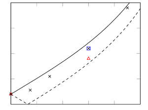
Figure 8(a) shows the pre-multiplied pressure PSD at the separation line for fixed shock strength and increasing sweep angle. The figure also shows the frequency spectra using a  $50\,\%$ shorter time window for the cases G00_T10, G30_T10 and G45_T10. All distributions exhibit a bump at the high-frequency end, which is associated with the boundary layer turbulence dynamics. In addition, they show prominent peaks at much lower frequency, which, however, are shifted to the right and increase in magnitude as the sweep angle grows. Although some difference may be spotted (especially for the G45_T10 flow case), we can confidently state that the limited duration of the time window does not affect the typical frequencies, and energy at the expected ‘two-dimensional’ characteristic frequency ( $St_L=0.03\unicode{x2013}0.04$) is negligible in cases with significant skewing of the flow. The model in (4.2) predicts two distinct frequencies, but one should regard those as broadband peaks that could well merge into one if sufficiently wide. Quantitative comparison of the numerically computed peak frequencies with the prediction of (4.2) is presented in figure 8(b), in which we also include results of DNS with different shock strength. The prediction is clearly quite good, perhaps with exception of the single data point corresponding to $\gamma _0 = 30^{\circ }$, $\theta = 8^{\circ }$, which features a relatively small separation bubble. Overall, we find that the agreement becomes more satisfactory as the sweep angle increases, which is consistent with stronger coherence of convecting pressure disturbances noticed when discussing figure 6.
(a) Pre-multiplied normalized frequency spectra of wall pressure at the mean separation line for various sweep angles and for fixed shock strength ( $\theta =10.4^\circ$). Peaks are marked with crosses. Solid lines denote PSD obtained with the full time window, whereas dashed lines denote PSD obtained with 50 % shorter time windows. (b) Peak frequency as a function of sweep angle: the solid and dashed lines denote the prediction of (4.2).

5. Discussion
We have developed a simple model to characterize low-frequency unsteadiness in swept SBLIs, which is robustly supported from analysis of DNS data. Although at the present stage we cannot offer a complete mechanistic justification for our observations, we provide a scaling law for the spanwise undulation of the separation line and for the convection velocity of pressure disturbances, which concur to predict growth of the typical pressure oscillation frequency with the skew angle, consistent with trends observed in DNS. One should, of course, bear in mind that the present database refers to the idealized case of a statistically two-dimensional flow with addition of cross-flow, which is representative of SBLIs with cylindrical symmetry (Gross & Fasel Reference Gross and Fasel2016).
However, SBLIs in practical occurrences almost invariably feature conical symmetry. Hence, a crucial question is whether and to what extent our findings and predictions actually apply to realistic occurrences of swept SBLIs. In this respect we note that the two key elements which we have identified as being responsible for the observed low-frequency unsteadiness, namely spanwise undulation of the separation line and convection of pressure disturbances, have been observed previously in several studies of swept SBLIs. In fact, the presence of ripples in the instantaneous separation line was first pinpointed in the studies of Vanstone et al. (Reference Vanstone, Saleem, Seckin and Clemens2017) and Vanstone & Clemens (Reference Vanstone and Clemens2019). They found that these structures move at approximately 70–80 % of the cross-stream velocity, hence well in line with the present study. However, they reported the typical width of the ripples to be approximately half the incoming boundary layer thickness, hence much less than we find here, and to contribute to a relatively high-frequency range of pressure fluctuations.
Rippling of the separation line was also noticed by Doehrmann et al. (Reference Doehrmann, Padmanabhan, Threadgill and Little2018), Adler & Gaitonde (Reference Adler and Gaitonde2020) and Padmanabhan et al. (Reference Padmanabhan, Maldonado, Threadgill and Little2021). The latter study reports that the rippling motion is associated with low-frequency dynamics at spanwise-constant characteristic frequency, and that it corresponds to disturbances being advected at speed increasing with the spanwise distance, hence with increasing wavelength. A rather unconsolidated scenario emerges, which can be partially explained with effects of incomplete similarity in SBLIs with conical symmetry, and/or with differences from one SBLI case to another.
If the results of the present study are extended directly to swept interactions with conical symmetry on a station-by-station basis, one would infer that undulations of the separation line should have a wavelength proportional to the distance from the virtual origin, and be convected at constant speed. The resulting low-frequency peak would then scale with the local separation bubble size, and the peak frequency should decrease with the spanwise distance. Whereas this scenario is fully consistent with the findings of Erengil & Dolling (Reference Erengil and Dolling1993), it is a bit hard to reconcile it with more recent experiments (Padmanabhan et al. Reference Padmanabhan, Maldonado, Threadgill and Little2021).
It should finally be mentioned that only few experimental and numerical studies of swept SBLIs cover a wide range of sweep angles, including small ones. In fact, Erengil & Dolling (Reference Erengil and Dolling1993) noted that ‘ $\ldots$ increase in dominant frequencies is initially small as the interaction is swept from 0 to $20^{\circ }$ but becomes more rapid with increasing sweep ( $25^{\circ }$)’. Hence, additional studies in the range of small sweep angles would be desirable to establish whether the change from two- to three-dimensional dynamics is continuous, or characterized by a sharp transition.
Acknowledgements
We acknowledge that the results reported in this paper have been achieved with computational resources from PRACE Research Infrastructure resource MARCONI100 based at CINECA, Casalecchio di Reno, Italy. A.C. wishes to acknowledge Lionel Larchevêque for support and useful discussions during a secondment at the University of Aix-Marseille.
Funding
This work was supported by TEAMAero Horizon 2020 research and innovation programme under grant agreement 860909 and by the Air Force Office of Scientific Research under grants FA9550-19-1-0210 and FA9550-19-1-7029.
Declaration of interests
The authors report no conflict of interest.
Data availability statement
The datasets generated during and/or analysed during the current study are available from the corresponding author on reasonable request.


 Open access

