


Introduction
The ongoing global climate change affects the Arctic more than the rest of the globe (Serreze and Barry, Reference Serreze and Barry2011). The current changes in Arctic sea ice (Perovich and others, Reference Perovich2019; Pörtner and others, Reference Pörtner2019) are of major relevance for shipping companies, fishery, oil and gas industry, ecosystems and local residents. Understanding these ongoing changes, in particular the decrease in sea-ice thickness (Ricker and others, Reference Ricker2017a; Reference Ricker2017b) and sea-ice extent (Meier and others, Reference Meier2014; Perovich and others, Reference Perovich2019), are essential to better understand global climate processes (Budikova, Reference Budikova2009; Liu and others, Reference Liu, Curry, Wang, Song and Horton2012; Vihma, Reference Vihma2014). Ground-based electromagnetic (EM) sea-ice thickness profilers have now long demonstrated their capacities (Kovacs and Morey, Reference Kovacs and Morey1991; Haas and others, Reference Haas, Gerland, Eicken and Miller1997) and paved the way to airborne electromagnetic instruments (AEM) (Kovacs and others, Reference Kovacs, Valleau and Holladay1987; Haas and others, Reference Haas, Lobach, Hendricks, Rabenstein and Pfaffling2009). AEM surveys are now playing an important role in the field for regional- and large-scale monitoring of the sea ice (Lindsay, Reference Lindsay2010; Hendricks and others, Reference Hendricks2011; Lindsay and others, Reference Lindsay2012; Renner and others, Reference Renner2014; Haas and Howell, Reference Haas and Howell2015; King and others, Reference King2017; Rösel and others, Reference Rösel2018a). The flying speed and range allow a fast and extended measurement of the regional distribution of sea-ice thickness (Renner and others, Reference Renner2014; King and others, Reference King2017; Rösel and others, Reference Rösel2018b), which could not be obtained by any other means. It also avoids an underestimation of thinner ice and leads fraction which may occur, for safety reasons, on land-based surveys. However, the sea ice may exhibit a substantial surface anisotropy and, in particular, long linear features, such as leads and ridges, aligned on a general direction. These features can be undersampled if their broader scale is not estimated properly, or conversely overrepresented if a significant part of the flight follows a particular feature. Identifying the true size of 2-D features with 1-D transects is a well-known problem (Key, Reference Key1993; Horvat and others, Reference Horvat2019) as well as the potential error induced in the resulting sampling (Key and Peckham, Reference Key and Peckham1991).
Flight plans are usually prepared based on available sea-ice maps, which depend on available and updated remote-sensing products. But in a complex and dynamic environment such as sea ice, it is not always easy to identify the best route to get the most representative sampling of the area. Given that expeditions, and in particular flying hours, are costly, it appears essential to optimise procedures as much as possible.
In this study, we first investigate the extent to which sea-ice anisotropy can affect AEM surveys. Two different approaches have been tested to evaluate the effect of anisotropy, first using a radial analysis around the centre point of an image, then by simulating random flight lines over the images. In both cases the distribution of the ice classes has been calculated for each line and analysed in regard of their flight trajectories. We then propose an automated processing, based on the flight-line simulations, of sea-ice maps to identify which flight directions would be preferred to get survey lines that are most representative for sea-ice conditions in the actual region at the given time.
Data and method
Study area
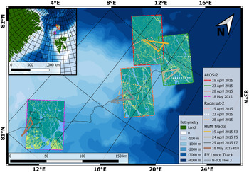
In this study, we focus on the area of the Norwegian young sea ICE expedition (N-ICE2015), in the Arctic Basin north of Svalbard. In particular, we will use the data collected during the drift of so-called Floe 3, lasting from 18 April 2015 to 5 June 2015 (Granskog and others, Reference Granskog2016). We chose this phase of the drift experiment because it included a helicopter to conduct airborne sea-ice thickness surveys, and satellite acquisitions were planned to overlap the surveys. Figure 1 shows the drift track of the ice station.

Fig. 1. Map of the study region, along with footprints for satellite images used in this study (dashed and dotted lines, see legend for details). The ALOS-2 segmented images are shown with light blue for open water and thin ice class, teal for level ice and yellow for deformed ice. The Radarsat-2 (RS-2) images are only presented here with their footprints for a better readability of the map. Finally, the overlapping AEM tracks are overlaid on the SAR satellite images. The background shades of blue represent the bathymetry (from shallower in light blue to deeper in dark blue).
The sea ice in the vicinity of Floe 3 consisted of three main ice types: thin ice of refrozen leads (RL), first year ice (FYI) and second year ice (SYI), with modal total thickness of 0.2, 1.2 and 2.3 m, respectively (Rösel and others, Reference Rösel2016a), according to ground surveys conducted in the vicinity (within a 5 km radius) of the R/V Lance. Ice types were identified by ice-core salinity and isotope analyses, in combination with sea-ice thickness data (Granskog and others, Reference Granskog2017). Snow thickness was on average 0.45 m on thicker ice types (Rösel and others, Reference Rösel2016b), while on the RL it was ~0.02 m, consisting of blowing snow adhering to frost flowers on the surface (Rösel and others, Reference Rösel2016b). Back-trajectory analysis for the ice station showed that the oldest sea ice might originate from September 2013 from the northern Laptev Sea and is thus considered to be SYI (Itkin and others, Reference Itkin2017).
Similarly, the ice core analysis from Granskog and others (Reference Granskog2017) indicated that the sea ice in the area consisted mainly of only FYI and SYI, interrupted by RL with young ice and pressure ridges. Rösel and others (Reference Rösel2018a) presented a simplified ice classification of the area with three classes ‘thin’ (comprising open water and RL), ‘level’ and ‘deformed’ ice, with the respective fraction of each class: 11, 74 and 14%. For an ease of comparison between remote-sensing imagery and AEM survey, we use here a similar classification of the ice.
Sea-ice thickness and surface roughness from airborne surveys
As part of the N-ICE2015 campaign, 16 helicopter-borne regional ice surveys over Floe 3 and sea ice in the vicinity were conducted in the period of 15 April 2015 to 18 May 2015 (King and others, Reference King, Gerland, Spreen and Bratrein2016). Results of the campaign are so far published in Rösel and others (Reference Rösel2018a), Itkin and others (Reference Itkin2017), Johansson and others (Reference Johansson2017) and King and others (Reference King2018). In this study we use total sea ice and snow thickness measurements (further referred to as ‘sea-ice thickness’ for simplicity) and surface roughness estimates along the flight tracks obtained using AEM instrument, towed under a helicopter. Here we will use the definition of the roughness as derived from the radar meaning of the term: the std dev. of the local surface elevation (Ulaby and others, Reference Ulaby, Moore and Fung1982).
The ice thickness sensor, presented in detail by Haas and others (Reference Haas, Lobach, Hendricks, Rabenstein and Pfaffling2009), makes use of the principles of EM induction at the seawater/sea-ice interface. Using a set of transmitting and receiving coils it allows deriving the distance from AEM to the bottom of the sea ice. A Riegl LD90-3100HS laser altimeter mounted in the AEM additionally provides the distance from the instrument to the top of the ice, or snow surface in the case of snow-covered sea ice. Over level sea ice, the accuracy of the AEM measurements was found to lie within ± 0.1 m of drillhole measurements (Haas and others, Reference Haas, Lobach, Hendricks, Rabenstein and Pfaffling2009). The instruments footprint in regular operating conditions, with a helicopter flight altitude of ~40 m, is of ~50 m (Kovacs and others, Reference Kovacs, Holladay and Bergeron1995; Beamish, Reference Beamish2003; Renner and others, Reference Renner2014). This suggests that the inferred thickness of ice ridges, which are narrower than the instrument's footprint, is often underestimated. Whenever possible, in addition to the AEM data, we used imagery from a helicopter-mounted automatic camera (GoPro) that recorded overlapping images of the flight track every 2 s to aid a visual interpretation of the AEM data, in particular identification of leads and open water.
Surface roughness along the flight paths is calculated using the laser altimeter of the AEM, which offers a ± 15 mm accuracy of the measured distance. The sampling rate of the laser is set to 100 Hz. With a typical flying speed of 30–40 m s −1, the sampling distance varies from 30 to 40 cm.
This altimeter was not intended for surface topography measurement, in particular, it has no inertial measurement unit. The distance measured is relative to the AEM and is therefore affected by the helicopter movements. As it is impossible to fly the helicopter perfectly parallel to a reference surface, such as sea level, the distance recorded is heavily affected by the changes in altitude, in addition to the surface signal. The surface profile, and therefore the surface roughness, cannot be directly interpreted from the signal recorded. The helicopter movements have to be removed by filtering first.
In broad outline, the signal is a superposition of a high frequency component from the height variations of the sea-ice surface and a low frequency component from the helicopter movement. Therefore, retrieving the ice surface topography consists of isolating the helicopter motion using a low-pass filter and subtracting it from the laser altimeter signal. To filter the helicopter movement, we followed a three-step filter proposed by Hibler III and others (Reference Hibler, Weeks and Mock1972), commonly used in such applications (Beckers and others, Reference Beckers, Renner, Spreen, Gerland and Haas2015; Yitayew and others, Reference Yitayew2018). An example of the filtering is shown in Figure 2. On this 2 km segment of the flight, we can see the estimated motion of the aircraft and the resulting surface topography. Without elements of comparison, it appears impossible to quantify the accuracy of the filter. Aside from few exceptions (e.g. ~1100 and 1450 m in Figure 2, possibly cracks in the sea ice, or filtering artefacts), the reconstructed surface profile looks credible.
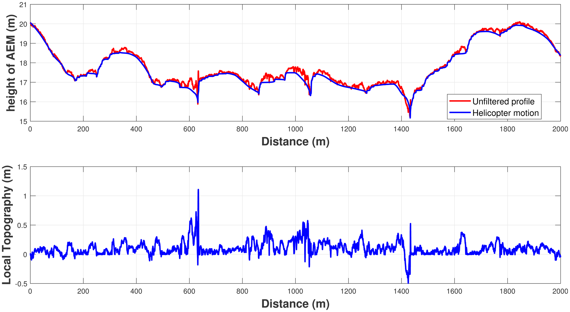
Fig. 2. Example of the filtering of the helicopter movement on a 2 km section of the flight from 24 April 2015. The top figure presents the altimeter profile recorded by the AEM (in red) and the estimated aircraft motion (in blue). The resulting estimation of the surface topography is presented in the bottom figure, relative to the mean surface elevation.
Once the surface topography is obtained, we estimated the surface roughness by calculating the std dev. of the surface on a sliding window of 200 points, corresponding roughly to the AEM footprint of 50 m. Finally, the sea-ice roughness is segmented in two classes of roughness. As the histograms of surface roughness only present one mode (Fig. 3), the boundaries between the smooth and rough classes was chosen arbitrarily based on the average roughness for each flight (0.045 m for 19 April 2015, 0.041 m for 24 April 2015, 0.051 m for 29 April 2015, 0.032 m for 18 May 2015).
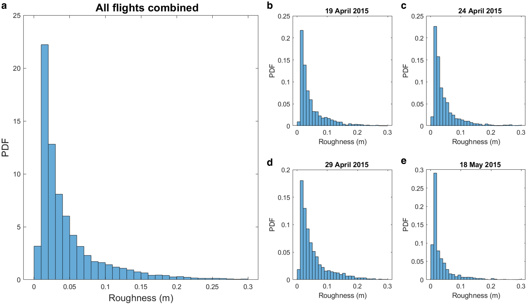
Fig. 3. Histograms of the surface roughness as estimated from the four airborne surveys on 19 April 2015, 24 April 2015, 29 April 2015 and 18 May 2015. The histogram on the left represents the histogram of the four flights combined together.
The AEM data are also classified, according to the thickness, into two classes: thin ice and thick ice. The thickness threshold between thin and thick ice can be subject to discussion. For simplicity, and taking into account that some AEM surveys only present one thickness mode (King and others, Reference King, Gerland, Spreen and Bratrein2016; Rösel and others, Reference Rösel2018a), we chose to base the threshold on the lowest point between the two main modes in the overall AEM sea-ice thickness distribution: 0.6 m (Fig. 4). The AEM data are then classified into three ice classes, combining roughness and thickness segmentation: (1) thin ice: ice under 0.6 m of thickness; (2) level ice: ice over 0.6 m thick and below average roughness; (3) deformed ice: ice over 0.6 m thick and above average roughness.

Fig. 4. Histograms of the ice thickness as measured during the four airborne surveys on 19 April 2015, 24 April 2015, 29 April 2015 and 18 May 2015. The histogram on the left represents the histogram of the ice thickness for the four flights combined together. The red vertical line represents the limit of 0.6 m chosen to separate thin and thick ice.
Satellite data
This study is based on L-band (ALOS-2) and C-band (RS-2) fine quad-polarisation synthetic aperture radar (SAR) satellite remote-sensing data acquired during the N-ICE2015 expedition. Their processing and classification aim to assess the general ice situation and identify the best airborne survey strategy. A total of seven images overlapping with AEM flights have been processed, four ALOS-2 and 3 RS-2, acquired on 19 April 2015, 23 April 2015 and 28 April 2015 for both ALOS-2 and RS-2 (ALOS-2 and RS-2 images overlapping on each dates), and 18 May 2015 with ALOS-2 only.
The satellites images are high-resolution quad-polarimetric SAR images, acquired at 1.2 GHz (ALOS-2) and 5.41 GHz (RS-2) (Johansson and others, Reference Johansson2017). The difference in the operation frequencies results in differences in the retrieved back-scattering. C-band SAR images are commonly used in sea-ice monitoring for extent, concentration and drift speed (Maillard and others, Reference Maillard, Clausi and Deng2005; Walker and others, Reference Walker, Partington, Van Woert and Street2006; Karvonen and others, Reference Karvonen, Simila and Lehtiranta2007). L-band SAR has, more recently, also demonstrated its value in monitoring Arctic sea ice (Lehtiranta and others, Reference Lehtiranta, Siiriä and Karvonen2015). In particular, it appears more efficient than C-band in discriminating deformed ice from level ice (Dierking, Reference Dierking2009; Eriksson and others, Reference Eriksson2010). In this study we chose to process these two types of images identically (with the same algorithm and settings, independently from their characteristics) to set ourselves in the most general configuration possible.
The images have been segmented using a Gaussian mixture model clustering algorithm developed by Doulgeris and Eltoft (Reference Doulgeris and Eltoft2009); Doulgeris (Reference Doulgeris2013). The segmentation algorithm separated each image into unlabelled categories which had to be interpreted. Although the algorithm may fail over complex parts of the images, where the ice presents heterogeneous properties, it allows a rigours clustering of similar areas of a scene (Moen and others, Reference Moen2013). The algorithm has been set up for a ‘generic’ ice segmentation: it was not tuned for any specific purpose (e.g. ice versus open water or thin ice versus thicker ice) but to discriminate as many segments as possible. In such configuration for quick processing, we do not expect the segmentation to be perfect and some segments may exhibit ambiguity and ice class mixing. Our goal is to preserve the main sea-ice features and keep them easily recognisable. The similar segments are merged together, for easier reading and analysis, and labelled into three main ice classes ((1) open water and thin ice – further called thin ice for simplicity–, (2) level ice and (3) deformed ice), based on the direct field observations as well as the Pauli false-colour versions of the SAR satellite images.
The ALOS-2 image from 23 April 2015 is frequently used as an example in the analysis below. The area covered by this particular image features clear networks of ridges and freshly opened leads. It is also the one exhibiting the least ambiguity in the classification.
Spatial analysis of the SAR satellite images
Radial analysis
As a first approach, we investigate the orientations of sea-ice features by analysing the percentage of each ice class along a simulated transect for each degree of azimuth (relative to the geographical north) around the central point of the image. In order to simulate the footprint of the AEM the fractional coverage of each ice class is calculated in a 100-m wide buffer along the flight path. As one would expect, this first analysis clearly shows strong directional differences of the sea-ice features for the example chosen (Fig. 5). The distribution of the classes can significantly change according to the direction of the flight.

Fig. 5. Fraction of each class (thin, level and deformed) against the azimuth (relative to the north) for the ALOS-2 from 23 April 2015 (radial analysis).
We can notice several peaks for the thin ice class and some azimuths (e.g. ~90°) where the deformed ice class disappears completely from the sampling. In particular, the azimuths between 210° and 235° demonstrate two major peaks and a generally higher fraction of thin ice (36% of thin ice, Fig. 5). If a transect were to be made with this azimuth, we would get a measurement of the area with a poor representation of the area abundances. The scene-average areal coverage of each class is 12% (9), 75% (9) and 12% (6) for thin, level and deformed ice, respectively, with numbers in parenthesis showing the associated std dev.
The analysis points to the azimuth of 200° to be most representative of the whole image (on average 11% of thin ice, 72% of level ice and 17% of deformed ice and ridges).
However, this method presents two main shortcomings. First, each azimuth is sampled only once and covers only half of the image from the centre point. This can be heavily biased by possible regional effects, which is highlighted by the absence of an expected 180° rotational symmetry. Second, the centre area of the image is oversampled compared to the outer parts of the image.
Random flight simulations
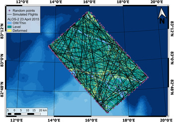
In order to obtain an optimised representation of the area, we further elaborate a method of flight path simulation along random azimuth lines. The flight lines are simulated by generating random points on the edge of the SAR satellite image and connecting all possible pairs. The number of points varies from 170 to 297 between the SAR scenes, due to constraints introduced in the generation algorithm, such as restricted area on the edge of the images and a minimum distance of 200 m between points. In total, ~15 000 to 20 000 lines are generated for each SAR scene. Figure 6 presents an example of the proposed approach, showing for a better visualisation a randomly selected subset of 100 generated lines. The points shown on the outer edge form a complete set used in generating the entire set of simulated flight tracks. In this particular case, 183 points yield a total of 16 653 simulated flight paths.

Fig. 6. Example of 100 randomly generated flight paths over the ALOS-2 image from 23 April 2015. All randomly generated points (purple circles) on the outer edge are the points used to generate all the flight paths.
This approach may present a bias as the length of simulated lines varies. To investigate the impact of transect length on the variance of the surveyed ice classes, we simulated lines of flight of fixed length (ranging from 1 to 30 km), covering the whole SAR image, and parallel to the range direction of the images (longer side on ALOS-2 images, to ensure optimal cover of the image and longer transects). For every length of the flight track, we then calculated the std dev. of the ice classes distribution. Figure 7 presents the evolution of the std dev. as a function of transect length. The RS-2 image from 19 April 2015 is not presented in the figure because, with only two ice classes, the std dev. is the same for the two classes and does not change above 5 km. For all but one scene, the inter-class variability generally decreases with increasing transect length. The ALOS-2 scene from 28 April 2015 demonstrates an opposite pattern with a rapid increase of the std dev. of the thin and level ice classes with a maximum ~12 km transect length (Fig. 7c). We do not have an explanation for this particular case.

Fig. 7. Evolution of the std dev. of each class against the length of the simulated flight lines for the six different satellite images used. The legend for all the sub-figures can be found in sub-figures (f).
The set of randomly generated lines is then cleaned by filtering out the lines on the outer edge of the image (containing more than 50% of ‘no data’ values), or lines shorter than 20 km. This threshold is chosen based on our general procedure when planning a survey. It also fits the results shown in Figure 7. After having applied these criteria, ~25% of the generated transects are further excluded from analysis. In order to simulate the AEM footprint, the percentage of each ice class is then calculated in a 100-m wide buffer along the simulated flight line. The results are presented on a cumulative area distribution, binned by degree of azimuth. For each azimuth, we took the average fraction of each class and calculated the corresponding std dev. Figure 8 shows the example of ALOS-2 from 23 April 2015.

Fig. 8. Distribution of the sea-ice classes under the simulated flight paths, according to the flight path azimuth, for the ALOS-2 image from 23 April 2015. The lines have been binned by 1° azimuth. The grey bands represent the std dev. of each ice class (scaled down by a factor 3 for readability).
Results
Empirical interpretation
Both analyses conducted on the segmented images revealed a clear directional anisotropy of the distribution of ice classes. The random flight tracks approach shows a 180° rotational symmetry in the distribution, whereas this is not apparent in the radial approach. This difference is due to design of the experiment: in the radial analysis each line only covers half of the image, from the centre to the edge, while the lines are crossing the whole image in the random analysis. The latter approach also enables a more complete coverage of the different sub-regions of the image.
Detailed analysis of the results suggests that some flight directions appear to have a more homogeneous distribution of the ice classes than others (Fig. 9). This is linked with regional features; e.g. Figures 1 and 6 demonstrate that RL and ridged ice is more frequent in the southern half of the scene.

Fig. 9. Close up view of a 20° band of azimuth for a homogeneous area (left) and highly variable area (right) on the ALOS-2 image from 23 April 2015 (random analysis). The grey bands represent the std dev. of each class (scaled down by a factor 3 for readability).
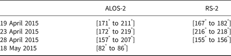
On the ALOS-2 image from 23 April 2015, for a range of azimuths the fraction of thin ice is significantly increased. A strong directional anisotropy of leads and a RL contributes to thin ice fraction maxima ~140° and 150° of azimuth. The deformed ice class also presents peaks (e.g. between 50° and 60°), but it is overall less noticeable than the thin ice class. We can also note that within these azimuths the inter-class variability is generally higher than between 0° and 20° (Table 1). Major leads and ridges tend to prevail on the southern half of the image. Any line in the southern half would therefore capture a bigger proportion of leads and ridges than in the northern part of the scene. This has to be taken into account while creating flight plans.
Table 1. Comparison of class variability for two different 20° azimuth bands, as shown in the figure

Looking at the temporal evolution (Fig. 10), we can see the change of the main leads and ridges orientation as well as the general ice conditions. On 19 April 2015, the ridges present a much more abundant class than leads, which are barely present. This is confirmed by the segmented SAR images (Fig. 1). Apart from leads near the eastern and southern edges of the image, barely any can really be seen in the rest of the scene. Due to ice divergence in the study area, the leads appear more frequently on 23 April 2015 and become even more dominant on 28 April 2015. We can also see an overall change in the main orientation of the leads, globally rotated ~15° counter-clockwise.

Fig. 10. Distribution of the sea-ice classes under the simulated flight paths, according to the flight path azimuth, for all four ALOS-2 images. The grey bands represent the std dev. of each class (scaled down by a factor 3 for readability).
A major storm was recorded in the observation area between 25 April 2015 04.00 UTC and 27 April 2015 23.00 UTC with a peak wind speed up to 12.6 m s −1 (Cohen and others, Reference Cohen, Hudson, Walden, Graham and Granskog2017). Unfortunately, the weather station on the ice was not in operation before the 23 April 2015 10.00 UTC. The reference 10-m wind speed measurement has been reconstructed using the data from the ship anemometer (Hudson and others, Reference Hudson, Cohen and Walden2015; Cohen and others, Reference Cohen, Hudson, Walden, Graham and Granskog2017). Looking at the data, two events, in the afternoon of 19 April 2015 and the afternoon of 20 Aprl 2015, could be considered as storms, with 11.1 and 12.5 m s −1 peak wind speed, respectively. This can be considered the main driver for the observed changes in the state of sea-ice cover between 19 April 2015 and 28 April 2015. In particular, this explains the significant increase of the open water classes we can notice in a sequence of three images from 19 April 2015 (Fig. 10a), 23 April 2015 (Fig. 10b) and 28 April 2015 (Fig. 10c). Finally, on 18 May 2015, no clear homogeneous area really appears anymore (Fig. 10). In particular in the southern half, the ice pack appears significantly more broken with distinctive ice floes drifting apart (Fig. 1).
In contrast to ALOS-2, the segmentation algorithm, in its current configuration, applied to RS-2 images resulted in a poorer discrimination of the ice types into the segments (Fig. 11). In particular, thin ice and deformed ice could often be mixed in the same segment with implications for the general capacity of the method to identify best flight patterns. The resulting classification is therefore biased and may alter our capacity to identify the best lines of flight. Though this could easily be solved by adjusting the algorithm parameter, e.g. via increasing the numbers of segments, our motivation was to keep the experiment as generic as possible to get closer to the operational situation.

Fig. 11. Distribution of the sea-ice classes under the simulated flight paths, according to the flight path azimuth, for all three RS-2 images.
Despite this class mixing, we can notice a similar pattern on 19 April 2015 between the ALOS-2 and the RS-2 images. The level and deformed ice classes proportion are more stable between 160° and 180° of azimuth. On 23 April 2015, these features are barely visible and totally non-existent on 28 April 2015. This may highlight the importance of spatial features conservation.
Automated interpretation of the ice type distributions
Here we aim to identify the ranges of azimuths presenting an ice type distribution the closest to the average over the whole image with the lowest variance. The visual interpretation of the processed SAR satellite images already gives a good idea on the directions one could prefer when planning a flight. But in some cases, like for 28 April 2015 for the RS-2 image or 18 May 2015 for the ALOS-2 image, this empirical interpretation can be complicated, if not impossible.
We here propose a metric to identify which azimuths and hence potential flight directions are the closest to the image-averaged ice classes distribution. We first calculate the overall median percentage of each class in the image and then we calculate the mean, and the corresponding std dev., over a 5° azimuth sliding window. The distribution of mean values obtained against the azimuth is then compared with the overall median for each class. The difference between the two is multiplied by the associated std dev. The std dev. is used here as a weighing parameter to discriminate azimuths close to the overall ice types distribution, with the lowest variance. The values are finally normalised to be compared. This metric value is assigned to the corresponding azimuth for each ice class. For each ice class, we define a set of azimuths as valid for having a metric below the arbitrarily chosen threshold of 0.1. This threshold may need to be adjusted depending on the results obtained and the user's expectations. Finally, an intersection of the three derived sets of valid azimuths yields the ranges of valid lines of flight for a given analysed SAR satellite image (Table 2).
Table 2. Ranges of azimuth for potential flight paths considered as representative for the area for all satellite images
All the ranges have a 180° counter-parts (due to rotational symmetry) not noted here.
For the ALOS-2 images, the results obtained are, in most cases, consistent with the empirical estimation. It must be noted that we had to lower the validation threshold to 0.05 to avoid too many results on the image from 18 May 2015. With a standard threshold many isolated azimuths are considered validated, making the final choice more difficult to achieve. Another solution could be to increase the size of the sliding window from 5° to 10°, for example.
Although consistent with ALOS-2, the results are not as satisfactory for the RS-2 images. The segmentation resulted in more class mixing, leading to an overall higher variance in the ice classes. This introduce more noise in our metric and makes the identification of a valid range more complicated. In order to limit the analysis output, we had to lower the threshold to eliminate the validated individual azimuths. The result for 19 April 2015 also remains consistent with our empirical analysis.
Discussion
Radial versus random lines approaches
The random lines approach, as of now, is computationally intensive and hence currently not practical for operational planning of flights. On a regular laptop computer, it takes between 24 and 48 h, for one image, to compute where the radial analysis only takes few minutes. The radial analysis method, though more efficient computationally, does not provide an even coverage; a bias around the pivot point makes it unsuitable for the purpose.
We can expect the computing time issue of the random line approach to be improved in the future with optimisation of the code, in particular using parallel processing, and more powerful computers. The random line approach gave the desired results, helping us identify the most representative azimuths for a survey in the area. However, it remains dependent on the image segmentation to give proper results.
Segmentation and classification of the SAR satellite images
The segmentation of the SAR satellite images plays an important role in the identification of the optimal line of flight. While the segmentation algorithm gave overall good results on the L-band images (as visually compared to Pauli false-colour images), the C-band images resulted in a substantial variability of ice types in some segments. In particular, RL partly or entirely covered with frost flowers could be mixed up with deformed ice, explaining a higher deformed ice proportion.
In an attempt to make the results easier to understand and interpret, we merged the different ice segments into three main ice classes (the number of initial segments varying between the images from 3 to 9). Even if it appeared sufficient in our study, in particular for ALOS-2, this classification was not done by a trained sea-ice analyst and may results in misinterpretation of some segments. This point can be improved with training and experience of the user.
Although coarsely classified into three ice types, the analysis conducted on the images let us identify the optimal lines of flight in all ALOS-2 images. It is interesting to notice that the RS-2 image from 19 April 2015 is the only one able to give proper results among RS-2 images, while it is also the one with the least number of initial ice segments from the segmentation algorithm (only 3). Distinguishing between leads and ridges for this scene was not possible with the current settings of the segmentation algorithm. This can be a major issue if for a particular scene the spatial distributions of these two ice classes are anisotropic and directionally different. But in this case, considering that the selected azimuths are consistent with the ALOS-2 image from the same date, the segmentation appears sufficient for the purpose. The proper classification of the sea ice may not be a major criterion when it comes to processing them for the purpose of survey planning, as long as the main features are preserved. In order to assist the classification procedure, we suggest to visually compare the segmented image to a Pauli false-colour image (e.g.) instead of putting more effort and time in the classification of the image. If the main features appear preserved, the segmentation can be considered good enough as it is for this purpose. Since this assessment relies on the user's ability to interpret polarimetric SAR images, we suggest some training prior to an expedition, in such SAR image interpretation or, if possible, the assistance of a trained person.
Comparison of simulated tracks with actual AEM data
This method could be derived to make post-flight assessments of airborne surveys. All satellite scenes selected for this study were acquired within one day from the AEM surveys conducted in the study area, allowing the comparison between the two. The flight tracks were corrected for the ice pack drift, using the ship positions as a reference and the time difference between the flight and satellite acquisition. We here assume that relative motions between ice floes are negligible over the time difference and the ship drift is representative of the local ice pack drift. As the flights were conducted following a triangular pattern, each segment of a flight with a main direction was analysed separately. To be compared with the SAR satellite data, the AEM data are cropped to match the footprint of the satellite. The ice type distribution for each flight leg is presented in Table 3.
Table 3. Percentage of ice classes for each leg of each helicopter flight, later used for the comparison with the simulated AEM surveys
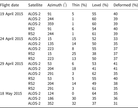
Each date had only one single flight. Each line of the table represents one flight leg, with its corresponding azimuth. The legs are cropped to fit the corresponding SAR satellite image.
For the images from 19 April 2015, 23 April 2015 and 28 April 2015, one of the flight legs has an azimuth considered as representative for the ALOS-2 acquisitions. None of the flight legs are matching azimuths with a low metric value for the RS-2 images. The comparison of the AEM data to the ALOS-2 data highlights two main differences. The deformed ice class is either systematically underrepresented in the satellite-based analysis, or overestimated in the AEM data (Table 4). This could be explained by the threshold used to differentiate deformed ice from level ice in the AEM data. The derived surface roughness probability densities are unimodal (Fig. 3) and the threshold had to be chosen arbitrarily. Setting an arbitrary threshold to differentiate level from deformed ice should influence the result. Furthermore, the definition of ice classes in the two datasets differs significantly, in particular with respect to the surface roughness estimation procedure. The laser altimeter of the AEM offers a limited spatial sampling of ~0.3 m, which is conditional on the AEM operational speed. This allows capturing bigger structures on the ice surface, such as ice ridges. On the other hand, as mentioned previously, frost flowers can be mixed with deformed ice in the SAR satellite data, due to a high backscatter (Isleifson and others, Reference Isleifson2014; Johansson and others, Reference Johansson, Brekke, Spreen and King2018), while being mostly invisible for the laser altimeter. While in the AEM data analysis, the thickness of the ice is directly measured and used for the classification, in SAR satellite data analysis, ice thickness is inferred from image segmentation, the Pauli false-colour and the field observations. This can lead to differences in thin/thick distribution between SAR and AEM classifications. This supports the importance the identification of the ice spatial features, in the SAR satellite data, over a proper classification of the sea ice.
Table 4. Comparison of the ice classes distribution in AEM data and ALOS-2 data
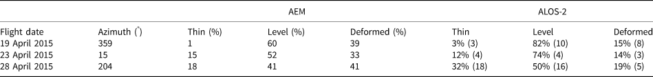
The associated std dev. is shown in parenthesis.
It must be noted that the flight leg from 23 April 2015, representing a proportion of thin ice the most similar to the SAR data is also the longest of the three: 25 km against 10 km and 16 km for 19 April 2015 and 28 April 2015, respectively. Longer transects allow an averaging of potential local clustering, or lack, of ridges and/or leads. For instance, we can see that almost no thin ice was flown over during the survey on 19 April 2015. Then, the spatial scale of leads occurrence can be higher than 10 km, and this class can therefore be underrepresented, compared to the broader area. In such cases, we would then advise to plan longer transects, or adjust the flight directions within the triangle such that they fall into the identified ranges of representative azimuths, if circumstances allow.
Limitations
The proposed procedure has so far only been tested on the N-ICE2015 data. Though the sea-ice cover in the area has been subject to dynamic changes over the study period, the ice seen on the SAR satellite images was overall the same between the different images, as the satellite acquisitions were planned to follow the drift of the ship. The time difference between AEM surveys and satellite acquisitions has been up to 18 h. With the observed ice drift and ice divergence in the study area, it was sufficient to hinder an alignment of the flight tracks with the satellite scenes, thus making a pixel-based comparison of the two datasets inaccurate. We can expect that in more dynamic areas or periods, the time gap between the satellite acquisition and the actual flight needs to be minimised down to a few hours to get meaningful results.
In the proposed version of the method, we simulated AEM surveys as lines connecting the random pairs of points drawn on the edges of the satellite scenes. This introduces a bias as all the segments have different lengths, and also differ in length from the actual AEM survey transects. An option could then be to define a fixed length for the simulated transects and repeat the pattern over the whole image. It appears to us that the main challenge of this approach is the identification of the optimal length and its applicability in a real case scenario. However, simulating survey lines with a range of lengths has a clear benefit too. In particular, as presented in Figure 7, the variance of the different ice classes tends to converge to lower values with longer simulated transects. This is why we selected longer transects and simulated a large set of survey lines to average the ice types distribution for each given azimuth.
Here, we considered the whole scene as representative of the regional area and a reference for planning an AEM survey. The variability of the ice on the scale of a satellite scene affects what one could consider representative of the area. A satellite image remains a local snapshot of the ice situation and the sea ice in the image is also affected by wider scale ice conditions. As we could see on the ALOS-2 scene from 23 April 2015, the southern half of the image differs significantly from the northern half. In such a case, one could choose to only consider a subset of the image as a reference to plan an AEM survey, or on the opposite use a broader area, provided for example by a wide swath images.
For this study we used high-resolution quad-pol SAR images, which due to their size cannot always be immediately available for operational applications in remote areas. Systematic acquisition, free access and short delivery time makes, e.g. Sentinel-1 wide swath images more suitable for these kinds of applications. Noise and the limitation to dual-polarisation are the main issues affecting the segmentation of a wide-swath image. This, however, is an active field of research for many groups and constant progress is made in this research area. We are confident our proposed method will soon be usable also with wide-swath dual-pol SAR images.
Conclusions
At present, AEM surveys represent almost the only option for high-resolution ice thickness surveys from local to regional spatial scales. Proper flight planning based on remotely sensed observations of the regional ice cover can help optimise the survey and ensure that the results more accurately represent the ice cover.
Based on segmented satellite SAR imagery, we investigated the effect of the floe-scale anisotropy on AEM surveys. By simulating multiple flight lines over SAR satellite images we demonstrated how variable the results of different surveys could be. As expected, the analysis confirmed that a flight track configuration have an implication for representativeness of the survey, a given flight may not be representative for the area covered by a satellite image.
We used the simulation of flight lines to estimate the optimal azimuth to survey a given area, by calculating the representativeness of each azimuth. The metric we proposed to evaluate this representativeness of the different azimuths is weighted with the spatial variability of given azimuths. We would then avoid directions which have different characteristics between different areas of the image (for example ensuring crossing of leads and ridges in any parts of the image). In this study, we only investigated long transects, crossing the image, and we recommend such long transects, when possible, to limit the effect of potential local bias (e.g. an heavily ridged area). If more than one flight direction are found optimal for the survey, they could be combined to plan a different flight pattern. In practice, we tend to limit the numbers of corners in the flight plan to keep the instrument as level as possible. Each turn of the aircraft induces a swing of the instrument and therefore an interruption in the measurement when the laser altimeter points off-nadir; hence a common use of triangular or bow-tie-shaped plans only presenting three and four turns respectively. The flight safety concerns, for example avoiding flights over wide leads, also have to be taken into account when planning a survey. Further developments could integrate these constraints and focus on identifying the best flight plan pattern to optimise the flight time and the data collected.
The method has only been tested in one region of the Arctic Basin, north of Svalbard, in spring conditions. Further investigations should be conducted over different sectors of the Arctic Basin and during different seasons. It has also been limited to quad-pol high-resolution SAR satellite imagery. In practice, wide-swath dual-pol images are acquired more frequently and offer a faster release which would make them more suitable for this purpose.
At present, the method is still computationally intensive. The code we produced for it has not yet been optimised and can be improved to run faster. In particular, the processing could be heavily parallelised and take advantage of modern multi-core processors to significantly reduce this issue. We can expect this to be solved soon.
In general, the main limiting factor in the application of our method remains the usually unavoidable time difference between the satellite acquisition and the airborne survey. Assuming the improvements of future remote-sensing products, and shortened product delivery time, we can expect the sea-ice maps to be available within few hours after their acquisitions. The maps could then be processed using our method to provide a preferred flight plan. Such processing could either take place on-board or on-land, depending on the available resources and competences. The resulting flight plan would then serve as a basis for the preparation of the actual survey.
Finally, this method could be derived to make post-flight assessments of airborne surveys and the region they took place in. In such case, the segmentation and the classification of the SAR images should go through a thorough examination to be considered as an accurate representation of the local ice situation.
Acknowledgments
We are grateful to the crew and scientists on board R/V Lance, in particular Jennifer King and Marius Bratrein (both NPI) who conducted the AEM surveys, as well as the helicopter pilots from Airlift AS. The authors wish to thank Max König (NPI) and Thomas Kræmer (UiT) who made the co-located satellite image acquisitions and AEM surveys possible. We also thank Anthony Doulgeris (UiT) who processed and segmented the images used in this study. This research is funded by ‘CIRFA’ (Center for Integrated Remote Sensing and Forecasting for Arctic operations) partners and the Research Council of Norway (CIRFA SFI grant no. 237906), and the Fram Center project ALSIM (Automised Large-scale Sea Ice Mapping) in the Fram Center ‘Sea ice in the Arctic Ocean, Technology and Governance’ flagship. This work has been supported by the Norwegian Polar Institute's Centre for Ice, Climate and Ecosystems (ICE) through the project N-ICE. The ALOS-2 Palsar-2 scenes were provided by JAXA under the 4th Research Announcement programme (PI: Torbørn Eltoft). The Radarsat-2 scenes were provided by NSC/KSAT under the Norwegian-Canadian Radarsat agreement 2015. N-ICE acknowledges the in-kind contributions provided by other national and international projects and participating institutions, through personnel, equipment and other support. N-ICE2015 data are available through the Norwegian Polar Data Centre at: https://data.npolar.no.


 Open access