


I. Introduction
Many empirical studies find a flat, hump-shaped, or negative relation between (physical) corporate distress risk proxies and stock returns (“distress anomaly”; see, e.g., Dichev (Reference Dichev1998) and Campbell, Hilscher, and Szilagyi (Reference Campbell, Hilscher and Szilagyi2008)).Footnote 1 In addition, Avramov, Chordia, Jostova, and Philipov (Reference Avramov, Chordia, Jostova and Philipov2022) find a negative relation between their ratings-based distress risk proxy and corporate bond returns. As they argue, the jointly nonpositive distress premiums cast a serious blow to existing theories aiming to rationalize the distress anomaly. More specifically, while Garlappi, Shu, and Yan (Reference Garlappi, Shu and Yan2008) and Garlappi and Yan (Reference Garlappi and Yan2011) claim that the distress anomaly arises from shareholders’ ability to extract rents from debtholders in distress (“shareholder advantage theory”; see also Favara, Schroth, and Valta (Reference Favara, Schroth and Valta2012), Hackbarth, Haselmann, and Schoenherr (Reference Hackbarth, Haselmann and Schoenherr2015), and Aretz, Florackis, and Kostakis (Reference Aretz, Florackis and Kostakis2018)), their theory predicts a positive—not negative—debt distress premium. Similarly, while Conrad, Kapadia, and Xing (Reference Conrad, Kapadia and Xing2014) claim that the anomaly arises from investors’ preference for positively skewed returns, their theory also fails to predict a negative debt distress premium. The depressing yet unavoidable conclusion is that we are back to square one in finding a rationale for the distress anomaly.
Our study offers a new rationale for the distress anomaly grounded in firms’ ability to disinvest real assets in distress (“disinvestment rationale”). We first establish that the anomaly does not only emerge in stocks and bonds but also emerges in traded loans and firm assets, measured, as in Choi (Reference Choi2013) and Choi and Richardson (Reference Choi and Richardson2016), as the value-weighted combination of stocks, bonds, and loans reflecting (real) assets. The negative premium in firm assets suggests that the anomaly could be driven by operational (and not financial) risk. To study that possibility, we allow for stock and debt claims in a standard real options model with capacity utilization, investment, and disinvestment choices (see Aretz and Pope (Reference Aretz and Pope2018)). Assuming that disinvestment proceeds are shared according to a fixed rule, the model reveals that the distress premium in a class becomes more negative with the proceeds paid out to that class and can be negative in both classes when debtholders receive the lion’s share but not all of the proceeds. Relying on proxies for the ease with which a firm can disinvest its hard assets, our empirical work supports our theory in showing that the bond and loan distress premiums become more negative with these proxies. Conversely, the stock premium often becomes less negative with them, possibly because shareholders benefit more from the sale of nonsecured hard assets.
We use Campbell et al.’s (Reference Campbell, Hilscher and Szilagyi2008) state-of-the-art distress proxy to show that the distress anomaly arises in stocks, bonds, loans, and firm assets.Footnote 2 In our stock–bond sample, our Fama and MacBeth (FM) (Reference Fama and MacBeth1973) regressions, for example, show that while the stocks in distress deciles 6–9 earn a 0.24% higher mean monthly return (t-stat: 2.61) than the lower-decile stocks, the top-decile stocks earn a 0.61% lower return (t-stat: −2.82) than the stocks in deciles 6–9. The corresponding numbers for bonds are −0.06% (t-stat: −4.10) and −0.25% (t-stat: −4.61), respectively. In our stock-bond-loan-asset sample, the same regressions reveal that while the decile 6–9 loans earn a similar mean monthly return as the lower-decile loans, the top-decile loans earn a 0.46% lower return (t-stat: −2.44) than the decile 6–9 loans. Given our evidence of hump-shaped or negative relations between distress and returns in the three classes, we unsurprisingly also find a nonpositive relation between distress and firm-asset returns, the value-weighted average of stock, bond, and loan returns.
Interestingly, while the negative premiums in the stock–bond sample remain significant for about half a year after portfolio formation, those in the stock-bond-loan-asset sample remain significant for only about 3 months. The reason could be that the stock-bond-loan-asset sample is tilted toward larger firms (as they are more likely to own traded loans), and larger firms are known to produce weaker asset pricing effects (Fama and French (Reference Fama and French2008)).
We conduct numerous robustness tests to verify our empirical results. In particular, we do rely on not only the month-end-to-month-end bond and loan returns used in most studies but also the alternative returns calculated from the first and last transaction price within a month in Bartram, Grinblatt, and Nozawa (Reference Bartram, Grinblatt and Nozawa2025). Moreover, we repeat our tests on data excluding matrix prices or reassigning surviving bonds or loans after a merger and acquisition (M&A) deal to the acquiror. While we consistently control for a comprehensive set of factors selected from the recent literature (see, e.g., Fama and French (Reference Fama and French2016), Dick-Nielsen, Feldhütter, Pedersen, and Stolborg (Reference Dick-Nielsen, Feldhütter, Pedersen and Stolborg2025), and Dickerson, Julliard, and Mueller (Reference Dickerson, Julliard and Mueller2026)), we further run separate tests also controlling for the bond illiquidity and bond liquidity risk measures of Bao, Pan, and Wang (Reference Bao, Pan and Wang2011) and Lin, Wang, and Wu (Reference Lin, Wang and Wu2011), respectively.Footnote 3 Finally, we use Compustat and Capital IQ data to show that while stocks, bonds, and loans capture about 70%–75% of the average firm’s asset value, trade credit is the one significant omitted liability class, making up about 12%–15% of that value.Footnote 4 Relying on arguments in Erens and Hoffmann (Reference Erens and Hoffmann2013) and Costello (Reference Costello2019) that trade credit is close to risk-free, we rerun our tests on asset returns calculated from stock, bond, loan, and (imputed) trade credit data. All robustness tests yield conclusions in complete agreement with our main empirical specifications.
In our theoretical work, we offer a new rationale for the jointly negative distress premiums in the four asset classes. Our rationale starts from the insight that many firms disinvest real assets in distress. Yet, as the ability to disinvest is akin to a real American put with a negative expected excess return (see Coval and Shumway (Reference Coval and Shumway2001)), it lowers the expected asset return, especially in distress (see Hackbarth and Johnson (Reference Hackbarth and Johnson2015), Aretz and Pope (Reference Aretz and Pope2018), and Gu, Hackbarth, and Johnson (Reference Gu, Hackbarth and Johnson2018)). To study if the ability to disinvest can also lower the expected stock and debt return, we extend the standard real options model of Aretz and Pope (Reference Aretz and Pope2018) by assuming that the firm is financed by not only stock but also a zero-coupon bond. Critically, we further posit that while the firm funds capacity expansions through equity, it distributes the proceeds from contractions to stock and debt claimants according to some fixed sharing rule. The logic is that the firm’s assets consist of easy-to-verify plausibly tangible secured assets and hard-to-verify plausibly intangible unsecured assets. While the firm is forced to pay out the proceeds from disinvesting secured assets to debt claimants, it can divert at least some fraction of the proceeds from disinvesting unsecured assets to stock claimants.
Our theoretical results suggest that the extended real options model can produce a negative relation between distress risk and expected stock or debt returns if the firm can disinvest its assets at a sufficiently high price. Fixing the disinvestment price, the relation between distress risk and the expected return to either claim becomes, in line with intuition, more negative the greater the fraction of disinvestment proceeds paid to that claim. Critically, the model can produce negative relations for both stock and debt when debtholders receive the lion’s share of disinvestment proceeds and shareholders some small residual.
We finally offer empirical support for the idea that disinvestment options add to the distress anomaly. To that end, we condition the distress premiums in stocks, bonds, and loans on well-known proxies for the ease with which firms are able to disinvest hard assets. More specifically, we rely on i) Gu et al.’s (Reference Gu, Hackbarth and Johnson2018) asset inflexibility; ii) Eisfeldt and Rampini’s (Reference Eisfeldt and Rampini2006) asset reallocation; iii) Schlingemann, Stulz, and Walkling’s (Reference Schlingemann, Stulz and Walkling2002) asset liquidity; and iv) Bai, Li, Xue, and Zhang’s (Reference Bai, Li, Xue and Zhang2025) investment skewness. We first validate these proxies by showing that distressed firms classified as owning more disinvestable hard assets indeed disinvest significantly more than their counterparts. More crucially, they create more negative bond and loan distress premiums, in line with the proceeds from selling such assets flowing (mostly) to debtholders. Strikingly, however, these firms yield a less negative stock premium. The reason may be that more difficult-to-disinvest hard assets are less likely to be used as collateral in debt contracts, allowing firms to channel (or tunnel) some proceeds from selling those assets to shareholders.
We add to studies on the distress anomaly. Dichev (Reference Dichev1998), Griffin and Lemmon (Reference Griffin and Lemmon2002), and George and Hwang (Reference George and Hwang2010) show that Altman’s (Reference Altman1968) z-score and Ohlson’s (Reference Ohlson1980) o-score, two accounting distress proxies, either do not or negatively price stocks. Deriving a distress proxy from Merton’s (Reference Merton1974) structural model, Vassalou and Xing (Reference Vassalou and Xing2004) instead find a positive stock distress premium, which is, however, largely driven by illiquid stocks (see Da and Gao (Reference Da and Gao2010)). Using the alternative structural model proxy of Moody’s KMV Corporation, Garlappi et al. (Reference Garlappi, Shu and Yan2008) and Garlappi and Yan (Reference Garlappi and Yan2011) find a downward hump-shaped relation between distress and stock returns. Using a distress proxy derived from a hazard model, Campbell et al. (Reference Campbell, Hilscher and Szilagyi2008) detect a negative stock distress premium. In accordance, Avramov, Chordia, Jostova, and Philipov (Reference Avramov, Chordia, Jostova and Philipov2009) find that stock returns are higher for firms with better credit ratings.Footnote 5 Closer to us, Avramov et al. (Reference Avramov, Chordia, Jostova and Philipov2022) jointly study stocks and bonds, reporting positive premiums for better rated firms in both. We contribute by jointly studying not only stocks and bonds but also loans, allowing us to estimate the firm-asset distress premium. We further distinguish ourselves from most studies by using the more recent proxy of Campbell et al. (Reference Campbell, Hilscher and Szilagyi2008).
We also relate to a literature aiming to explain the distress anomaly. Adding to Avramov et al. (Reference Avramov, Chordia, Jostova and Philipov2022), our empirical evidence that distress risk is negatively priced in loans and firm assets casts even greater doubts on Garlappi et al.’s (Reference Garlappi, Shu and Yan2008) and Garlappi and Yan’s (Reference Garlappi and Yan2011) shareholder advantage theory. The reason is that shareholders are more likely to renegotiate with private (rather than public) debtholders in distress since the Trust Indenture Act requires unanimous consent from all bondholders to modify bond terms. In the same vein, as bond and loan returns both become more negatively (rather than positively) skewed with distress risk, our loan evidence also casts greater doubts on Conrad et al.’s (Reference Conrad, Kapadia and Xing2014) conjecture that investors’ preference for positive skewness drives the distress anomaly. Conversely, our evidence aligns with O’Doherty’s (Reference O’Doherty2012) that distressed stocks have low market betas in recessions. While he, however, attributes those betas to uncertainty about the valuation of distressed firms, we would attribute them to disinvestment options. We contribute by proposing a novel rationale for the distress anomaly, also offering empirical evidence directly supporting it.
We finally add to an emerging literature studying loan and firm-asset returns. Using stock, bond, and loan data, Choi (Reference Choi2013) shows how firm-asset risk helps to explain the stock value premium, while Choi and Richardson (Reference Choi and Richardson2016) evaluate the pricing of the market beta, market size, book-to-market, and momentum in stocks and firm assets. Different from us, they, however, exploit loan data imputed from only 5 years of market loan data. Closer to us, Beyhaghi and Ehsani (Reference Beyhaghi and Ehsani2017) exclusively consider market loan data to examine the cross section of loan returns, showing that exposure to Fama and French’s (Reference Fama and French1993) credit risk factor does not robustly price that cross section. Using structural models to calculate firm-asset returns, Doshi, Jacobs, Kumar, and Rabinovitch (Reference Doshi, Jacobs, Kumar and Rabinovitch2019) establish that the market beta and size (but not book-to-market and volatility) price firm assets. Again relying on imputed loan return data, Bretscher, Feldhütter, Kane, and Schmid (Reference Bretscher, Feldhütter, Kane and Schmid2022) demonstrate that the value (leverage) premium exists in stock, bond, and firm asset but not loan returns (only in stockandbond returns). Exclusively using market loan data, we add to these studies by asking how Campbell et al. (Reference Campbell, Hilscher and Szilagyi2008) distress risk prices loans and firm assets.Footnote 6
We proceed as follows: While Section II details our variable definitions and data sources, Section III studies the pricing of distress risk in our asset classes. In Section IV, we show that a real options model with capacity utilization, investment, and disinvestment choices can explain our evidence in Section III. While Section V evaluates our theory’s new testable implications, Section VI sums up. We offer more variable details in the Appendix and theoretical derivations and additional/robustness tests in the Supplementary Material.
II. Methodology and Data
In this section, we offer variable definitions and describe our data sources. We first outline our two samples, the stock–bond and stock-bond-loan-asset samples, and detail how we calculate returns for each. We next explain how we calculate Campbell et al. (Reference Campbell, Hilscher and Szilagyi2008) distress risk. We offer additional details about the bond returns, the distress risk predictors used in Campbell et al. (Reference Campbell, Hilscher and Szilagyi2008), and our control variables in the Appendix.
A. The Playing Fields
1. The Stock-and-Bond Sample
Our stock–bond sample investigates the common stocks (shrcd: 10 and 11) of firms traded on the NYSE, AMEX, and Nasdaq (exchcd: 1, 2, and 3). While we directly source monthly stock returns from CRSP, we replace a stock’s return with its delisting return whenever the delisting return is nonmissing. If the delisting return is missing but the delisting code available, we replace that return with −30% for NYSE and AMEX stocks and −55% for Nasdaq stocks (see Shumway (Reference Shumway1997) and Shumway and Warther (Reference Shumway and Warther1999)). We exclude stocks with a 1-month-lagged price below $5 to mitigate market microstructure issues.
We rely on data from Lehman Brothers’ Fixed Income Database, Datastream, the Intercontinental Exchange (ICE), the Trade Reporting and Compliance Engine (TRACE), and Mergent’s Fixed Income Securities (FISD) and National Association of Insurance Commissioners (NAIC) databases to compute bond returns and characteristics. While the Lehman Brothers, Datastream, ICE, TRACE, and NAIC databases contain mostly bond market data, the FISD database features bond characteristic data, including the offering amount and date; the maturity date; the coupon rate, type, and frequency; the bond type, rating, and option features; and issuer information. We retrieve Lehman Brothers data over the start-1986 to end-1997 period,Footnote 7 Datastream data over the start-1990 to end-2006 period, ICE data from start-1996 to end-2004, NAIC data from start-1994 to end-2020, and TRACE data from July 2002 to end-2020.Footnote 8 To align our stock-and-bond data, we choose the sample period from January 1986 to December 2020 for the stock–bond sample, consisting of 420 monthly observations (35 years).
While we directly source monthly bond returns from the Lehman Brothers database, we calculate the return of bond $ i $
over month
$ i $
over month $ t $
,
$ t $
, $ {r}^B $
, from Datastream data as
$ {r}^B $
, from Datastream data as $ {RI}_{i,t}/{RI}_{i,t-1}-1 $
, where
$ {RI}_{i,t}/{RI}_{i,t-1}-1 $
, where $ RI $
is the total return index, and
$ RI $
is the total return index, and $ t $
consistently indicates the entire period for flow (e.g., the return over month
$ t $
consistently indicates the entire period for flow (e.g., the return over month $ t $
) but the end of the period for stock (e.g., the index value at the end of month
$ t $
) but the end of the period for stock (e.g., the index value at the end of month $ t $
) variables. We follow Bessembinder, Kahle, Maxwell, and Xu (Reference Bessembinder, Kahle, Maxwell and Xu2009), Choi (Reference Choi2013), and Choi and Richardson (Reference Choi and Richardson2016) in calculating that return from NAIC, ICE, and TRACE data as
$ t $
) variables. We follow Bessembinder, Kahle, Maxwell, and Xu (Reference Bessembinder, Kahle, Maxwell and Xu2009), Choi (Reference Choi2013), and Choi and Richardson (Reference Choi and Richardson2016) in calculating that return from NAIC, ICE, and TRACE data as
 $$ {r}_{i,t}^B=\frac{P_{i,t}+{AI}_{i,t}+{C}_{i,t}}{P_{i,t-1}+{AI}_{i,t-1}}-1, $$
where $ P $
is the bond price,
$ P $
is the bond price, $ AI $
is the accrued interest, and
$ AI $
is the accrued interest, and $ C $
is the coupon. In case of NAIC and TRACE, we construct
$ C $
is the coupon. In case of NAIC and TRACE, we construct $ {P}_{i,t} $
(
$ {P}_{i,t} $
( $ {P}_{i,t-1} $
) from the last 5 trading days of month
$ {P}_{i,t-1} $
) from the last 5 trading days of month $ t $
and, if no transactions occurred over those days, from the first 5 of month
$ t $
and, if no transactions occurred over those days, from the first 5 of month $ t+1 $
(the first 5 of month
$ t+1 $
(the first 5 of month $ t $
). See the Appendix for more details.
$ t $
). See the Appendix for more details.
A downside of our main method to calculate returns from NAIC and TRACE data is that if there are no bond transactions over the periods outlined previously, the return will automatically be missing. To mitigate that issue, we also follow the alternative methodology of Bartram et al. (BGN) (Reference Bartram, Grinblatt and Nozawa2025) to create returns. Arguing that, under lenient conditions, the dirty bond price follows a martingale under the physical measure, these authors choose the earliest (latest) dirty price over month $ t $
(month
$ t $
(month $ t $
plus the first 5 trading days of month
$ t $
plus the first 5 trading days of month $ t+1 $
) as proxy for the start (end) month price. They next proceed exactly as in our main methodology.
$ t+1 $
) as proxy for the start (end) month price. They next proceed exactly as in our main methodology.
We impose standard filters on our bond return data. First, we remove non-U.S. bonds. Second, we exclude structured notes; mortgage, asset, or agency-backed bonds; and equity-linked bonds. Third, we remove convertible or putable bonds. Fourth, we keep only fixed and zero-coupon bonds. Fifth, we remove bonds with less than a single year to maturity. Sixth, we exclude bonds with a market capitalization below $25 million at the start of month $ t $
and returns outside of the −100% to 100% range over that month. Seventh, in case of the TRACE bond data, we eliminate when-issued or locked-in transactions, those with special sales conditions, and cancelled, subsequently corrected, or reversed transactions.Footnote
9
$ t $
and returns outside of the −100% to 100% range over that month. Seventh, in case of the TRACE bond data, we eliminate when-issued or locked-in transactions, those with special sales conditions, and cancelled, subsequently corrected, or reversed transactions.Footnote
9
While the Lehman Brothers, Datastream, and ICE data contain bond quotes (first two) or matrix prices (all three), the NAIC and TRACE data contain transaction prices, with the NAIC data, however, only featuring those associated with the trades of insurance firms. As the consensus opinion is that transaction prices are more reliable than quotes, but that quotes are more reliable than matrix prices, we use the TRACE $ \succ $
NAIC
$ \succ $
NAIC $ \succ $
ICE
$ \succ $
ICE $ \succ $
Lehman Brothers
$ \succ $
Lehman Brothers $ \succ $
Datastream preference order in our bond return calculations.Footnote
10 We finally form a value-weighted portfolio of firm
$ \succ $
Datastream preference order in our bond return calculations.Footnote
10 We finally form a value-weighted portfolio of firm $ i $
’s outstanding bonds at the start of month
$ i $
’s outstanding bonds at the start of month $ t $
. As weight, we use either a bond’s market capitalization in case of the Lehman Brothers and Datastream data or the sum of its price and accrued interest times its outstanding number (calculated as the ratio of notional to principle amount) in case of the ICE, NAIC, and TRACE data.
$ t $
. As weight, we use either a bond’s market capitalization in case of the Lehman Brothers and Datastream data or the sum of its price and accrued interest times its outstanding number (calculated as the ratio of notional to principle amount) in case of the ICE, NAIC, and TRACE data.
In Section IA.1 of the Supplementary Material, we replicate all the exercises in the appendixes of Choi (Reference Choi2013) and Choi and Richardson (Reference Choi and Richardson2016) to confirm that our bond data are close-to-comprehensive and of a high quality. In particular, we show that although the bond sample is a relatively small (about 15%) subsample of the entire CRSP-Compustat universe featuring larger and more financially levered firms, it captures on average about 77% of the Compustat book debt of the included firms and about 85% of the outstanding balances in the entire FISD universe. Moreover, the sample contains an only small number of zero-price-change observations (1.70%); both firm- and portfolio-level returns constructed from it yield close-to-zero autocorrelations and cross-correlations with 1-month-lagged stock returns; and at least the ICE (but not necessarily Datastream) quotes are close to the corresponding NAIC and TRACE transaction prices (mean (median) difference: 0.87% (0.44%)).Footnote 11 Given that all these results align with those in the two studies previously, we also conclude that our bond sample is reasonably comprehensive and features a small but not major degree of staleness.
2. The Stock, Bond, Loan, and Firm-Asset Sample
For our stock-bond-loan-asset sample, we obtain data from Creditflux CLO-i, Refinitiv LoanConnector, and Reuters Dealscan to construct loan returns and fundamentals. While CLO-i contains loan transaction data from collateralized loan obligations (CLOs) starting from 2004, LoanConnector contains the bid–ask quotes of main dealers for secondary market loans starting from 1998.Footnote 12 Conversely, Dealscan provides loan characteristic data starting from the early 1980s. We use loan identification numbers (LINs) to merge the LoanConnector and Dealscan data. We rely on a matching algorithm based on firm and loan characteristics plus a manual verification to merge the LoanConnector/Dealscan with the CLO-i data.
Following Choi (Reference Choi2013), Choi and Richardson (Reference Choi and Richardson2016), and Beyhaghi and Ehsani (Reference Beyhaghi and Ehsani2017), we calculate the monthly return of loan $ i $
over month
$ i $
over month $ t $
,
$ t $
, $ {r}^L $
, as
$ {r}^L $
, as
 $$ {r}_{i,t}^L=\frac{Par_{i,t}{P}_{i,t}+\left({Par}_{i,t}-{Par}_{i,t-1}\right)+{AI}_{i,t}+{C}_{i,t}}{Par_{i,t-1}{P}_{i,t-1}+{AI}_{i,t-1}}-1, $$
where $ Par $
is the outstanding par value,
$ Par $
is the outstanding par value, $ P $
is the loan price,
$ P $
is the loan price, $ AI $
is the loan accrued interest on a 360-day basis, and
$ AI $
is the loan accrued interest on a 360-day basis, and $ C $
is the coupon, so that the second summand in the numerator on the right-hand side is the principle repayment over the month.Footnote
13 In line with standard data sources, we set
$ C $
is the coupon, so that the second summand in the numerator on the right-hand side is the principle repayment over the month.Footnote
13 In line with standard data sources, we set $ {P}_t $
(
$ {P}_t $
( $ {P}_{t-1} $
) to the transaction price on the last (first) trading day of the month if available and else to the bid–ask midpoint. Analogous to bonds, we also use the alternative methodology of BGN to calculate loan returns. As the bid–ask midpoint is, however, almost always available in our data, this strategy only marginally raises our sample size.
$ {P}_{t-1} $
) to the transaction price on the last (first) trading day of the month if available and else to the bid–ask midpoint. Analogous to bonds, we also use the alternative methodology of BGN to calculate loan returns. As the bid–ask midpoint is, however, almost always available in our data, this strategy only marginally raises our sample size.
Importantly, we highlight that, in contrast to several other studies, we do not impute the loan returns of firms with only nontraded loans from regressions of available loan returns on their corresponding bond returns and Treasury bond returns. We refrain from doing so since the justification for that strategy that loan values are far more stable than stock-and-bond values due to loans residing at the top of the capital structure is unlikely to hold for the loans of highly distressed firms, which are the main focus of our research.
We impose standard filters on our loan data. First, we drop non-U.S.-syndicated and non-U.S.-dollar loans. Second, we omit loans with less than 3 months to maturity. Third, we exclude loans with monthly returns outside the −100% to 100% range. We finally again form a value-weighted portfolio of all of firm $ i $
’s outstanding loans at the start of month
$ i $
’s outstanding loans at the start of month $ t $
, using a loan’s par value times the sum of its price (
$ t $
, using a loan’s par value times the sum of its price ( $ Par\times P $
) and accrued interest (
$ Par\times P $
) and accrued interest ( $ AI $
) as weight. We omit loan data before August 1999 to ensure wide enough cross sections. To align our stock-and-bond (calculated as in Section II.A.1) and loan data, we choose the sample period from August 1999 to April 2020 for the stock-bond-loan-asset sample, featuring 249 monthly observations (around 21 years). Critically, however, we retain a firm-month observation in that sample only if we have stock and loan (but not necessarily bond) data.
$ AI $
) as weight. We omit loan data before August 1999 to ensure wide enough cross sections. To align our stock-and-bond (calculated as in Section II.A.1) and loan data, we choose the sample period from August 1999 to April 2020 for the stock-bond-loan-asset sample, featuring 249 monthly observations (around 21 years). Critically, however, we retain a firm-month observation in that sample only if we have stock and loan (but not necessarily bond) data.
Section IA.1 of the Supplementary Material again follows Choi (Reference Choi2013) and Choi and Richardson (Reference Choi and Richardson2016) to evaluate the coverage and quality of our sample loan data. While the loan sample is an even smaller (about 3%) subsample of the CRSP-Compustat universe than the bond sample, it captures on average about 94% of Compustat book debt and about 12% of the outstanding balances in the Dealscan universe. Compared to the bond sample, the loan sample, however, features a much greater number of zero-price-change observations (33.91% vs. 1.70%); the portfolio (but not firm) level loan returns yield a higher first-order autocorrelation (0.43 vs. 0.10); and the firm-level returns share a higher cross-correlation with 1-month-lagged stock returns (0.15 vs. 0.06). Notwithstanding, as stressed by Choi and Richardson (Reference Choi and Richardson2016), the high proportion of zero-price-change observations may not indicate price staleness but rather stable expectations about interest rates and default risk. Also, the loan quotes are close to their corresponding transaction prices (mean (median) difference: 1.85% (0.51%)), and the cross-correlation of 0.15 implies an R 2 of only about 2% in a regression of loan returns on 1-month-lagged stock returns. Overall, we thus conclude that while our loan sample prices are more stale than our bond sample prices, the overall level of staleness is arguably still nonsevere.
We next follow Choi (Reference Choi2013) and Choi and Richardson (Reference Choi and Richardson2016) in appealing to Modigliani and Miller’s (Reference Modigliani and Miller1958) insight that the value of a firm’s real assets equals the value of its financial assets and approximate the firm’s (real) asset return as the value-weighted average of its stock, value-weighted bond-portfolio, and value-weighted loan-portfolio returns. To avoid bias arising from those bonds and loans excluded by our filters, we also include them in our calculations, assuming, however, that their returns equal those of their nonexcluded counterparts. In particular, let $ E $
be a firm’s stock market capitalization,
$ E $
be a firm’s stock market capitalization, $ B $
the sum of bond price plus accrued interest (
$ B $
the sum of bond price plus accrued interest ( $ P+ AI $
) times number of bonds outstanding taken over all its included and excluded bonds, and
$ P+ AI $
) times number of bonds outstanding taken over all its included and excluded bonds, and $ L $
the sum of par value times price plus accrued interest (
$ L $
the sum of par value times price plus accrued interest ( $ Par\times P+ AI $
) taken over all its included and excluded loans. Letting
$ Par\times P+ AI $
) taken over all its included and excluded loans. Letting $ MV $
be the sum of
$ MV $
be the sum of $ E $
,
$ E $
, $ B $
, and
$ B $
, and $ L $
, we then approximate firm
$ L $
, we then approximate firm $ i $
’s asset return over month
$ i $
’s asset return over month $ t $
,
$ t $
, $ {r}^A $
, as
$ {r}^A $
, as
 $$ {r}_{i,t}^A=\left(\frac{E_{i,t-1}}{MV_{i,t-1}}\right){r}_{i,t}^S+\left(\frac{B_{i,t-1}}{MV_{i,t-1}}\right){r}_{i,t}^{BP}+\left(\frac{L_{i,t-1}}{MV_{i,t-1}}\right){r}_{i,t}^{LP}, $$
where $ {r}^S $
and
$ {r}^S $
and $ {r}^{BP} $
are the stock and value-weighted bond return calculated as in Section II.A.1, respectively, and
$ {r}^{BP} $
are the stock and value-weighted bond return calculated as in Section II.A.1, respectively, and $ {r}^{LP} $
is the value-weighted loan return calculated as in this section.
$ {r}^{LP} $
is the value-weighted loan return calculated as in this section.
We acknowledge that our asset return proxy is imperfect because it ignores i) nontraded loans held by even those firms with traded loans and ii) nontraded liabilities. We later run robustness test showing that these imperfections do not greatly distort our conclusions.
B. The Pricing Variable: Corporate Distress Risk
We use Campbell et al.’s (Reference Campbell, Hilscher and Szilagyi2008) logit-hazard model to capture 12-month-ahead firm distress risk with only data available to investors at the time. To do so, we estimate a logit model of a dummy variable set to 1 if a firm defaults, files for bankruptcy, or delists for performance reasons over the month 12 months from the current, and else 0, Failure, on distress predictors at the end of the current month. We can compactly write that model as
 $$ \mathrm{Prob}\left({Failure}_{i,t}=1|{\mathbf{X}}_{i,t-12}\right)=\frac{1}{1+\exp \left(-\alpha -\boldsymbol{\beta} {\mathbf{X}}_{i,t-12}\right)}, $$
where $ \alpha $
is a parameter,
$ \alpha $
is a parameter, $ \boldsymbol{\beta} $
is a vector of parameters, and
$ \boldsymbol{\beta} $
is a vector of parameters, and $ \mathbf{X} $
is a vector encompassing the distress predictors. Consistent with Campbell et al. (Reference Campbell, Hilscher and Szilagyi2008), we estimate model (4) recursively, using data from start-January 1963 to end-December of calendar year
$ \mathbf{X} $
is a vector encompassing the distress predictors. Consistent with Campbell et al. (Reference Campbell, Hilscher and Szilagyi2008), we estimate model (4) recursively, using data from start-January 1963 to end-December of calendar year $ t $
, where
$ t $
, where $ t $
ranges from 1980 to 2008 in unit increments. We next combine the estimates from the estimation window stretching to the end of calendar year
$ t $
ranges from 1980 to 2008 in unit increments. We next combine the estimates from the estimation window stretching to the end of calendar year $ t $
with the distress predictor values over calendar year
$ t $
with the distress predictor values over calendar year $ t+1 $
. See the Appendix for more details about the default risk predictors.
$ t+1 $
. See the Appendix for more details about the default risk predictors.
We obtain the stock and accounting data required to compute the distress proxy from CRSP and Compustat. Yet, since we do not have access to Campbell et al.’s (Reference Campbell, Hilscher and Szilagyi2008) failure data, we cannot estimate logit model (4) ourselves. Fortunately, Jens Hilscher sent us the output from recursively estimating that model starting from 1980. We use the output obtained from his longest window, 1963–2008, to calculate the distress proxy for the post-2008 period. Doing so is unproblematic as his estimates strongly converge over time.Footnote 14
C. The Control Variables
We use a comprehensive set of controls in our portfolio sorts and FM regressions. In our portfolio sorts, we always start from simple factor models but then gradually expand these. In our stock sorts, we, for example, start from the Fama and French (FF3S) (Reference Fama and French1993) 3-factor model featuring the MKT, SMB, and HML. We next move to the Fama and French (FF5S) (Reference Fama and French2015) 5-factor model by adding RMW and CMA and then to the Fama and French (FF6S) (Reference Fama and French2016) 6-factor model by further adding MOM. Conversely, in our bond and loan sorts, we start from the Fama and French (FF5SB) (Reference Fama and French1993) 5-factor model featuring the MKT, SMB, HML, DEF, and TERM. We next move to an 8-factor model by adding an investment and a speculative-grade bond portfolio and bond momentum (SB8). We finally also add a parsimonious selection of bond factors chosen from recent bond pricing studies, as, for example, Dick-Nielsen et al. (Reference Dick-Nielsen, Feldhütter, Pedersen and Stolborg2025) and Dickerson et al. (Reference Dickerson, Julliard and Mueller2026), and including bond value, short- and long-term reversal, duration, and carry factors and the firm earnings announcement drift (SB14).Footnote 15 In our FM regressions, we use a comprehensive set of stock, bond, loan, and firm characteristics known to price our asset classes. See the Appendix for more details about our choice of controls and how we calculate them.
III. The Pricing of Corporate Distress Risk
In this section, we investigate the pricing of corporate distress risk. We first offer descriptive statistics. We next study the pricing of distress risk first in our stock–bond and then our stock-bond-loan-asset sample. We finally present robustness test results.
A. Descriptive Statistics
Table 1 offers descriptive statistics for our sample data. Panels A and B focus on the stock–bond and the stock-bond-loan-asset sample, respectively. The descriptive statistics include the number of observations (No. of Obs.), the mean, the standard deviation, and the first, 25th, 50th, 75th, and 99th percentiles, computed by sample month and then averaged over time. Panel A shows that the stock–bond sample contains an average of 3,480 stocks and between 764 (standard return) and 779 (BGN return) bond portfolios per month. Also, stocks attract both a higher monthly mean return (1.01% vs. 0.71%)Footnote 16 and standard deviation (12.27% vs. 2.33%) than bonds, and the average stock is larger than the average bond capitalization ($3.86 vs. $2.23 billion). Lastly, the average bond of the average sample firm has a bond market beta of 0.58, a time-to-maturity of about 10 years, and a credit rating close to BBB.
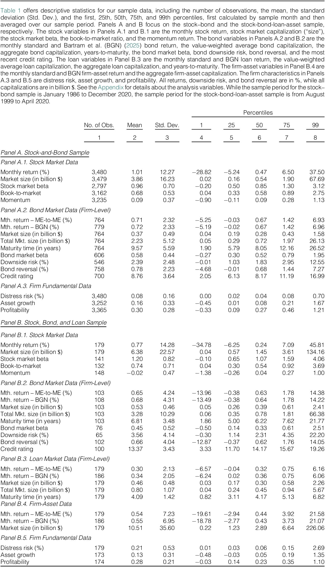
In contrast, Panel B reveals that the stock-bond-loan-asset sample contains an average of only 179 (standard return) or 186 (BGN return) firms per month because few firms own loans traded in secondary markets.Footnote 17 Contrasting stock-and-bond capitalizations across the samples, the stock-bond-loan-asset sample is heavily tilted toward larger firms. In line with the stock–bond sample, stocks have higher mean monthly returns (0.77% vs. 0.65%) and standard deviations (14.28% vs. 4.24%) than bonds, while bonds have higher mean returns (0.65% vs. 0.30%) and standard deviations (4.24% vs. 2.13%) than loans. Next, the average bond of the average sample firm has a lower bond market beta of 0.45, a shorter time-to-maturity of about 7 years, and a lower rating around B+ relative to the stock–bond sample. Conversely, the average loan of that firm has a market size of $0.80 billion and a time-to-maturity of about 4 years. Finally, the mean monthly asset return of about 0.54% lies between the mean monthly stock, bond, and loan returns (0.77%, 0.65%, and 0.30%, respectively).
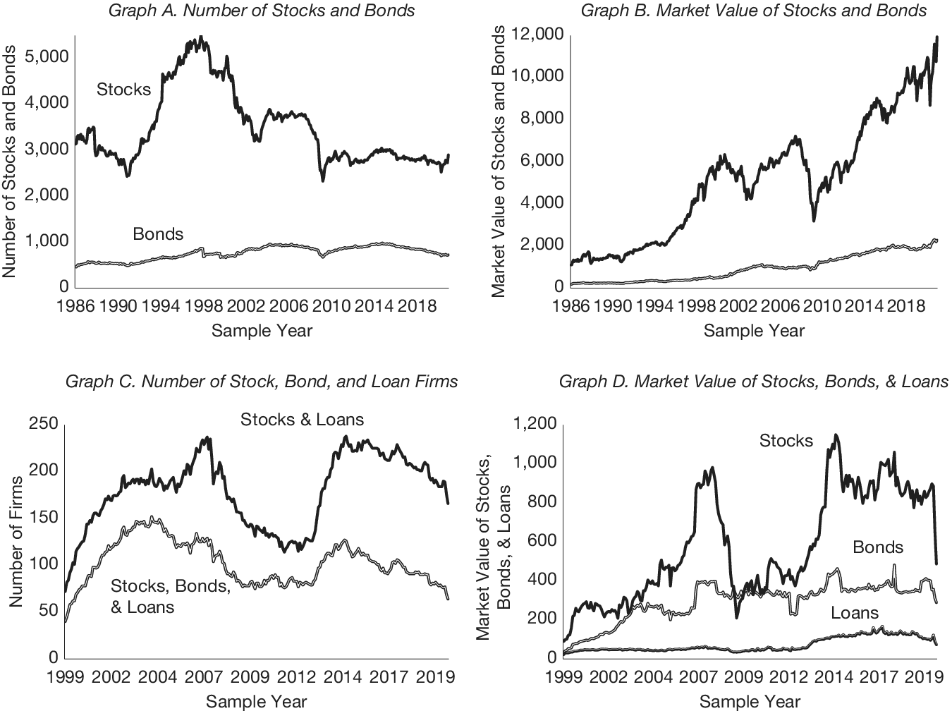
Figure 1 plots the numbers and aggregate capitalizations of the asset classes in our stock–bond (Graphs A–B) and stock-bond-loan-asset (Graphs C–D) samples, respectively. While Graph A shows that the stock–bond sample contains between about 2,300 and 5,500 stocks and between about 460 and 980 (firm-specific) bond portfolios, Graph B reveals that bonds make up between 10% and 20% of the aggregate stock-and-bond capitalization. Graph C suggests that the stock-bond-loan-asset sample contains between about 70 and 240 (40–152) firms with stocks and loans (stocks, bonds, and loans), representing only 2%–8% of the stock–bond sample. Finally, Graph D shows that the aggregate capitalization and its corresponding volatility are markedly higher for stocks than bonds, but then also markedly higher for bonds than loans.
Figure 1 plots the numbers and aggregate market capitalizations of the asset classes in our empirical work over our sample periods. While Graph A (B) shows the number of firms with stocks or bonds (the aggregate stock-and-bond capitalizations) in the stock–bond sample, Graph C (D) reports the number of firms with stocks and loans or stocks, bonds, and loans (the aggregate stock, bond, and loan capitalizations) in the stock-bond-loan-asset sample.
B. The Stock-and-Bond Sample
We next study the pricing of corporate distress in the stock–bond sample. We start with sorting our sample stocks or firm-specific bond portfolios into portfolios according to the decile breakpoints of Campbell et al.’s (Reference Campbell, Hilscher and Szilagyi2008) distress proxy at the end of month $ t-1 $
. We either value or equally weight the portfolios, where we use a firm’s stock capitalization or its aggregate bond capitalization to calculate the value weights. We hold the portfolios over month
$ t-1 $
. We either value or equally weight the portfolios, where we use a firm’s stock capitalization or its aggregate bond capitalization to calculate the value weights. We hold the portfolios over month $ t $
. For each set of portfolios, we create three spread portfolios to identify nonlinearities in the mean return-distress relation. While the first is long the middle (i.e., fifth) distress portfolio and short the bottom (“Middle–Low”), the second is long the top and short the middle (“High–Middle”) and the third long the top and short the bottom (“High–Low”). We risk-adjust by computing the intercept (“alpha”) from regressing portfolio excess returns on the factors of the models in Section III.C.
$ t $
. For each set of portfolios, we create three spread portfolios to identify nonlinearities in the mean return-distress relation. While the first is long the middle (i.e., fifth) distress portfolio and short the bottom (“Middle–Low”), the second is long the top and short the middle (“High–Middle”) and the third long the top and short the bottom (“High–Low”). We risk-adjust by computing the intercept (“alpha”) from regressing portfolio excess returns on the factors of the models in Section III.C.
Table 2 gives the portfolio sort results. While Panel A focuses on the stock and Panel B on the (firm-specific) bond portfolios, Panels B.1 and B.2 in Panel B report the spread portfolio results calculated from standard and BGN returns, respectively. While column 1 shows mean Campbell et al. (Reference Campbell, Hilscher and Szilagyi2008) distress risk, columns 2–5 (6–9) present the mean monthly returns and alphas of the value (equal)-weighted portfolios (all in %). Plain numbers are estimates, whereas those in square brackets are Newey and West (Reference Newey and West1987) t-statistics with a 12-month lag length. Panel A suggests that, in line with the literature, mean stock returns and alphas are hump shaped in distress risk, with them mildly rising over the first 8 deciles but sharply dropping over the last two. The value-weighted alpha of the most comprehensive factor model, the FF6S alpha, for example, rises mildly by 0.14% (t-stat: 0.89) over the first 5 deciles but then drops sharply by 1.12% (t-stat: −2.89) over the final 5 (see column 5). As a result, the drop in that alpha over the entire set of deciles is a less pronounced but still moderately significant −0.98% (t-stat: −2.25).
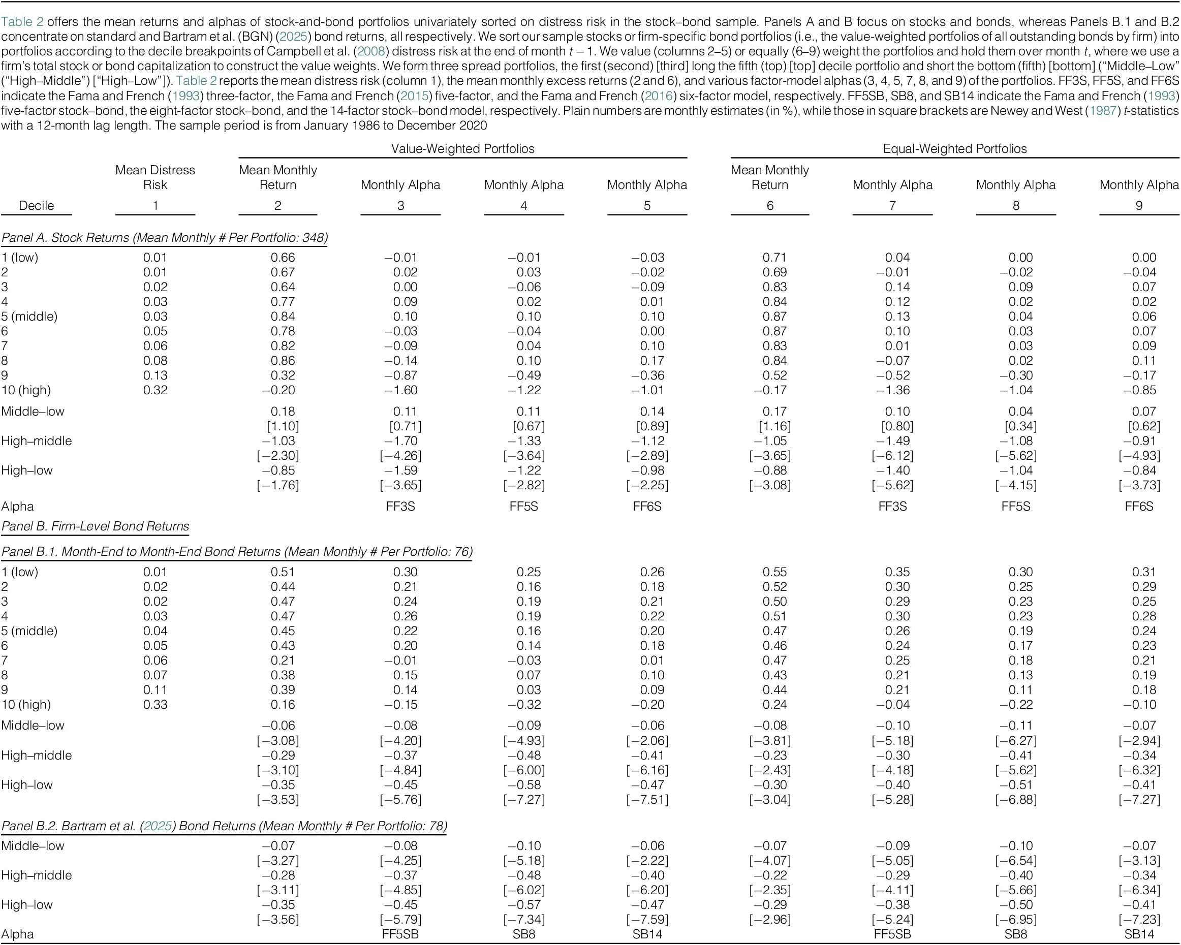
Panel B shows that mean bond returns and alphas decline more monotonically with distress risk, although the starkest drops again occur over the final deciles. The value-weighted standard-return alpha of the most comprehensive factor model, the SB14 alpha, for example, drops mildly by 0.06% (t-stat: −2.06) over the first 5 deciles but more sharply by 0.41% (t-stat: −6.16) over the final five (see column 5 in Panel B.1). Thus, the drop in that alpha over the entire set of deciles is an even stronger and more significant −0.47% (t-stat: −7.51). Contrasting the standard and BGN return results in Panels B.1 and B.2 reveals them to be close-to-identical, mostly due to the great overlap between the samples.
Table IA.4 and Figure IA.3 in the Supplementary Material report the mean characteristics and the factor loadings of the portfolios in Table 2, respectively. Both suggest that high-distress stocks tend to be small, unprofitable value stocks with high market betas, as also reported in prior studies. Conversely, high-distress bonds tend to be small, illiquid bonds with high speculative-grade bond market betas and coupon rates but low ratings and past returns. They also load more negatively on the earnings announcement factor than safer bonds.
In Table 3, we supplement our portfolio sorts with FM regressions explaining the month- $ t $
return. We run those regressions on the full stock sample in column 1 and the subsample of stocks with outstanding bonds in columns 2 and 3. Conversely, we run them on the full bond sample, the subsample of investment-grade bonds, and the subsample of speculative-grade bonds in columns 4 to 6, 7, and 8, respectively. We define as investment (speculative) grade bonds the value-weighted portfolio of all of a firm’s bonds with a rating equal to or above (below) BBB– at the start of month
$ t $
return. We run those regressions on the full stock sample in column 1 and the subsample of stocks with outstanding bonds in columns 2 and 3. Conversely, we run them on the full bond sample, the subsample of investment-grade bonds, and the subsample of speculative-grade bonds in columns 4 to 6, 7, and 8, respectively. We define as investment (speculative) grade bonds the value-weighted portfolio of all of a firm’s bonds with a rating equal to or above (below) BBB– at the start of month $ t $
. To capture nonlinearities, we use as main regressors two dummy variables calculated from our distress proxy, the first (second), HighDistress (LowDistress), set to 1 if the distress proxy takes on a value within the top decile (below the median) at the end of month ,
$ t $
. To capture nonlinearities, we use as main regressors two dummy variables calculated from our distress proxy, the first (second), HighDistress (LowDistress), set to 1 if the distress proxy takes on a value within the top decile (below the median) at the end of month , $ t-1 $
and else 0. In columns 3 and 5, we interact the distress dummies with a dummy variable set to 1 if the return of the other asset class is below the first quartile, and else 0, LowS/BRet. We further add the controls referred to in Section III.C. As always, plain numbers are monthly premium estimates (in %), whereas those in square brackets are Newey and West (Reference Newey and West1987) t-statistics with a 12-month lag.
$ t-1 $
and else 0. In columns 3 and 5, we interact the distress dummies with a dummy variable set to 1 if the return of the other asset class is below the first quartile, and else 0, LowS/BRet. We further add the controls referred to in Section III.C. As always, plain numbers are monthly premium estimates (in %), whereas those in square brackets are Newey and West (Reference Newey and West1987) t-statistics with a 12-month lag.
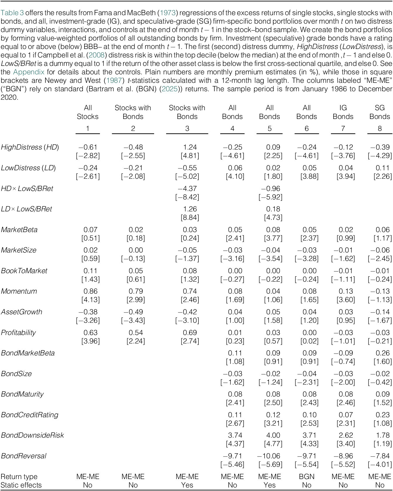
The FM regressions support our portfolio sorts by corroborating that mean stock returns are hump-shaped in distress risk but that mean bond returns decline more monotonically with it. Starting with the full stock sample, column 1, for example, shows that while the stocks in distress deciles 6–9 earn a 0.24% (t-stat: 2.61) higher mean return than those in deciles 1–5, the top-decile stocks earn a 0.61% (t-stat: −2.82) lower mean return than the decile 6–9 stocks. Conversely, column 4 reveals that the corresponding numbers for the full bond sample are −0.06% (t-stat: −4.10) and 0.25% (t-stat: −4.61), respectively. Noteworthily, column 2 suggests that the stocks-with-bonds subsample also produces a hump-shaped mean stock return-distress relation and columns 7 and 8 that the negative mean bond return-distress relation amplifies in the speculative-grade bond subsample.Footnote 18 In addition, the regressions featuring interactions with the other asset class in columns 3 and 5 suggest that distressed stocks (bonds) are more likely to underperform if the corresponding bonds (stocks) do so, too, refuting that one asset class exploits the other (as in the shareholder advantage theory). Finally, the standard and BGN returns again yield close-to-identical results, and the stock-and-bond controls produce premiums in agreement with the literature.Footnote 19
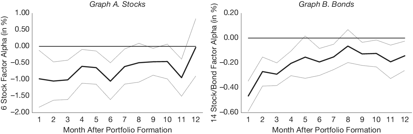
In Figure 2 and Table IA.5 in the Supplementary Material, we investigate the persistence in the stock-and-bond distress premiums in the stock–bond sample. Specifically, the figure plots the monthly FF6S stock (Graph A) and SB14 bond (Graph B) alphas of the value-weighted high-minus-low distress decile spread portfolios formed at the end of month $ t-1 $
plus their corresponding 95% confidence bands separately for each month from
$ t-1 $
plus their corresponding 95% confidence bands separately for each month from $ t $
to
$ t $
to $ t+11 $
. The table offers the same results plus the corresponding results from the equivalent equal-weighted spread portfolios and FM regressions. The figure and table suggest that the stock-and-bond distress premiums dissipate only slowly over time, with them being statistically significant at the 95% level or better for about half a year after portfolio formation.
$ t+11 $
. The table offers the same results plus the corresponding results from the equivalent equal-weighted spread portfolios and FM regressions. The figure and table suggest that the stock-and-bond distress premiums dissipate only slowly over time, with them being statistically significant at the 95% level or better for about half a year after portfolio formation.
Figure 2 plots the monthly FF6S stock (Graph A) and SB14 bond (Graph B) alpha of the value-weighted high-minus-low distress decile spread portfolio (sold line) and the corresponding 95% confidence bands (broken lines) separately for each of the first 12 months after portfolio formation (i.e., months $ t $
to
$ t $
to $ t+11 $
) in the stock–bond sample.
$ t+11 $
) in the stock–bond sample.
C. The Stock, Bond, Loan, and Firm-Asset Sample
We now study the pricing of corporate distress risk in the stock-bond-loan-asset sample. We again start with separately sorting our sample stocks, firm-specific bond portfolios, firm-specific loan portfolios, and firm-asset portfolios into portfolios according to the quintile breakpoints of Campbell et al.’s (Reference Campbell, Hilscher and Szilagyi2008) distress proxy at the end of month $ t-1 $
. We rely on quintile rather than decile breakpoints because the stock-bond-loan-asset sample is much smaller than the stock–bond sample due to it featuring only those firms with stocks and traded loans. The implication is that decile breakpoints sometimes yield ill-diversified portfolios. We again value or equally weight the portfolios and hold them over month
$ t-1 $
. We rely on quintile rather than decile breakpoints because the stock-bond-loan-asset sample is much smaller than the stock–bond sample due to it featuring only those firms with stocks and traded loans. The implication is that decile breakpoints sometimes yield ill-diversified portfolios. We again value or equally weight the portfolios and hold them over month $ t $
. Consistent with the prior section, we form three spread portfolios to identify nonlinearities in the mean return-distress relations, the first (second) [third] long the middle (top) [top] and short the bottom (middle) [bottom] portfolio (“Middle–Low,” “High–Middle,” and “High–Low,” respectively). We again risk-adjust by regressing excess portfolio returns on the factors of the same models as before.
$ t $
. Consistent with the prior section, we form three spread portfolios to identify nonlinearities in the mean return-distress relations, the first (second) [third] long the middle (top) [top] and short the bottom (middle) [bottom] portfolio (“Middle–Low,” “High–Middle,” and “High–Low,” respectively). We again risk-adjust by regressing excess portfolio returns on the factors of the same models as before.
Using a design analogous to Table 2, Table 4 gives the results from the portfolio sorts, with Panels A–C focusing on stocks, bonds, and loans, respectively. Panels A and B confirm that mean stock returns are hump-shaped in distress risk, while mean bond returns drop more monotonically with it. The value-weighted FF6S stock alpha, for example, rises by 0.46% (t-stat: 1.53) over the initial three quintiles but sharply drops by 1.58% (t-stat: −3.10) over the final three. The overall change is thus −1.12% (t-stat: −2.49). Conversely, the value-weighted standard-return SB14 bond alpha stays virtually constant over the initial three quintiles but sharply drops by 0.88% (t-stat: −3.58) over the final three. The overall change is thus −0.87% (t-stat: −3.52). Interestingly, Panel C suggests that traded loans are similar to bonds since their mean returns also drop monotonically with distress risk. The value-weighted standard-return SB14 loan alpha, for example, drops by 0.06% (t-stat: −1.88) over the initial three quintiles and 0.30% (t-stat: −2.66) over the final three. The overall change is thus −0.36% (t-stat: −2.89). The similar patterns for bonds and loans come as no surprise since both asset classes represent debt claims. Just like before, our inferences are close-to-identical across the standard and the BGN (bond or loan) return samples.
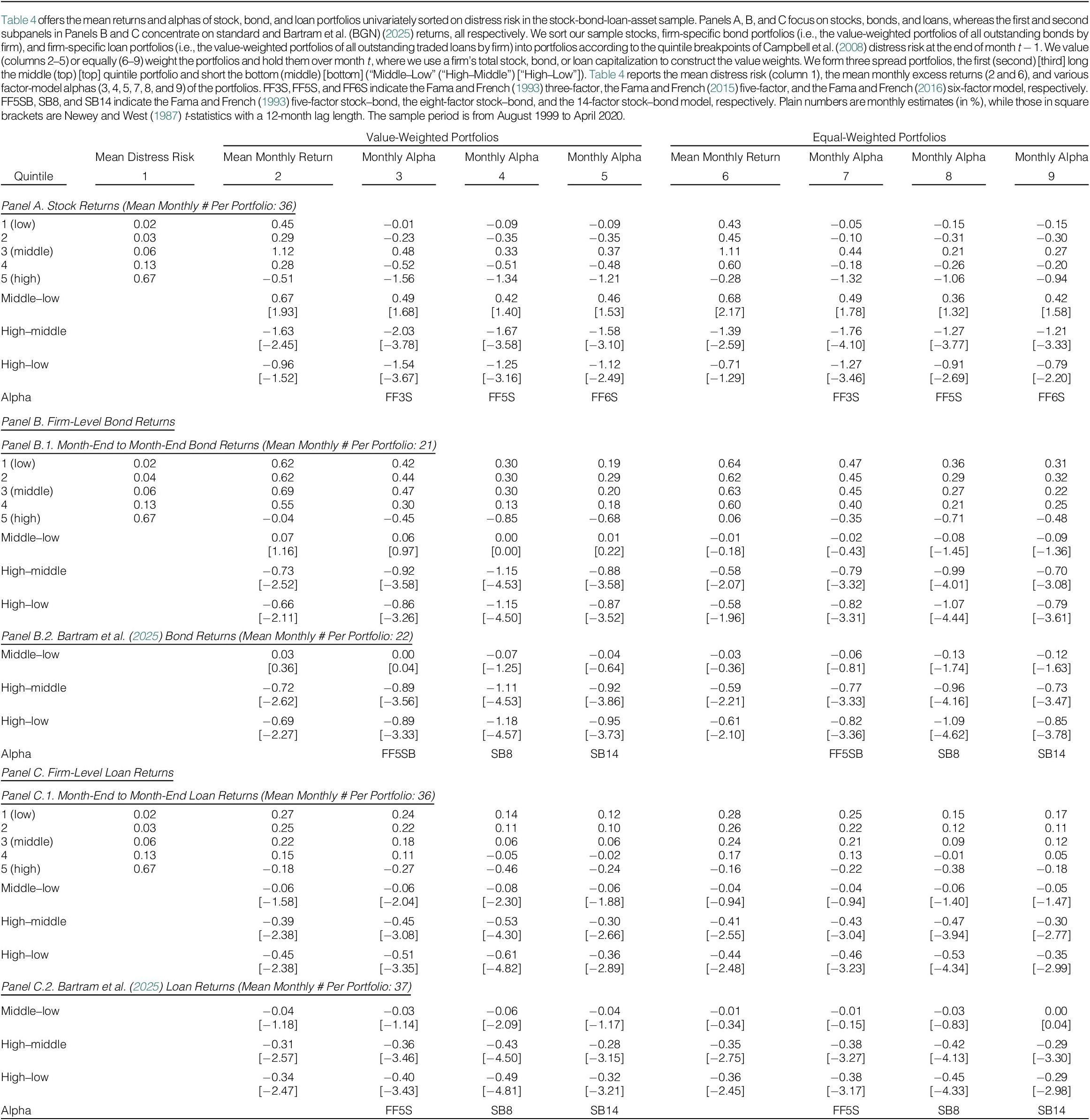
Table 5 offers the results from the portfolio sorts on firm assets, calculated as the value-weighted combination of stocks, bonds, and loans (recall equation (3)). The table shows that, similar to stocks, mean firm-asset returns are hump-shaped in distress risk, although the hump is less pronounced than for stocks. The value-weighted standard-return SB17 firm-asset alpha, for example, rises by 0.11% (t-stat: 0.50) over the initial three quintiles but drops sharply by 0.91% (t-stat: −3.59) over the final three. The overall change is thus −0.80% (t-stat: −2.64). The similarity between the stock and firm-asset results is largely due to i) the greater variations in mean stock relative to mean bond or loan returns over the quintiles, and ii) the greater weights associated with stocks than bonds or loans.
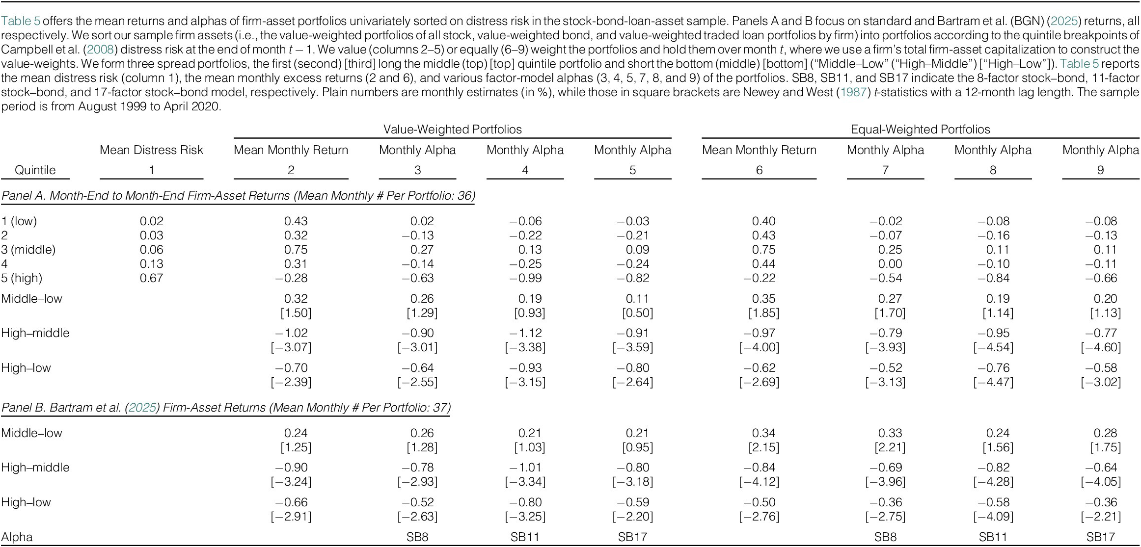
Table IA.7 and Figure IA.4 in the Supplementary Material present the mean characteristics and factor loadings of the portfolios in Tables 4 and 5, respectively. While both corroborate that the characteristics and loadings of the stock-and-bond portfolios largely agree across the stock–bond and the stock-bond-loan-asset sample, they further reveal that high-distress loans are short-maturity loans with low (i.e., negative) loadings on the default spread, the term spread, and the earnings announcement factors. Moreover, high-distress firm assets also command low loadings on the default spread and term spread factors but, interestingly, high loadings on the speculative-grade bond market portfolio and the bond value (HML) factor.
Using a design identical to Table 3, Table 6 once again supplements our portfolio sorts with FM regressions. The table confirms the relations of mean stock, bond, and loan returns with distress risk suggested by the portfolio sorts. While the stocks in distress deciles 6–9, for example, earn a 0.11% (t-stat: 0.37) higher mean return than lower-decile stocks, the top-decile stocks earn a 1.06% (t-stat: −2.23) lower mean return than decile 6–9 stocks (see column 1). Notwithstanding, the regressions yield more monotonically negative mean firm-asset return-distress risk relations. While the firm assets in distress decile 6–9, for example, earn a 0.02% (t-stat: −0.12) lower standard mean return than lower-decile assets, the top-decile firm assets earn a 0.79% (t-stat: −3.21) lower mean return than the decile 6–9 assets (see column 9). Similar to before, distressed stocks, bonds, or loans are more likely to underperform if the other asset classes do so, too, although the modulating effect is not always significant (see columns 2, 4, and 7). Finally, the standard and BGN returns again yield close-to-identical results, whereas most controls, however, do not produce significant premiums, likely due to the stock-bond-loan-asset sample’s tilt toward larger firms.
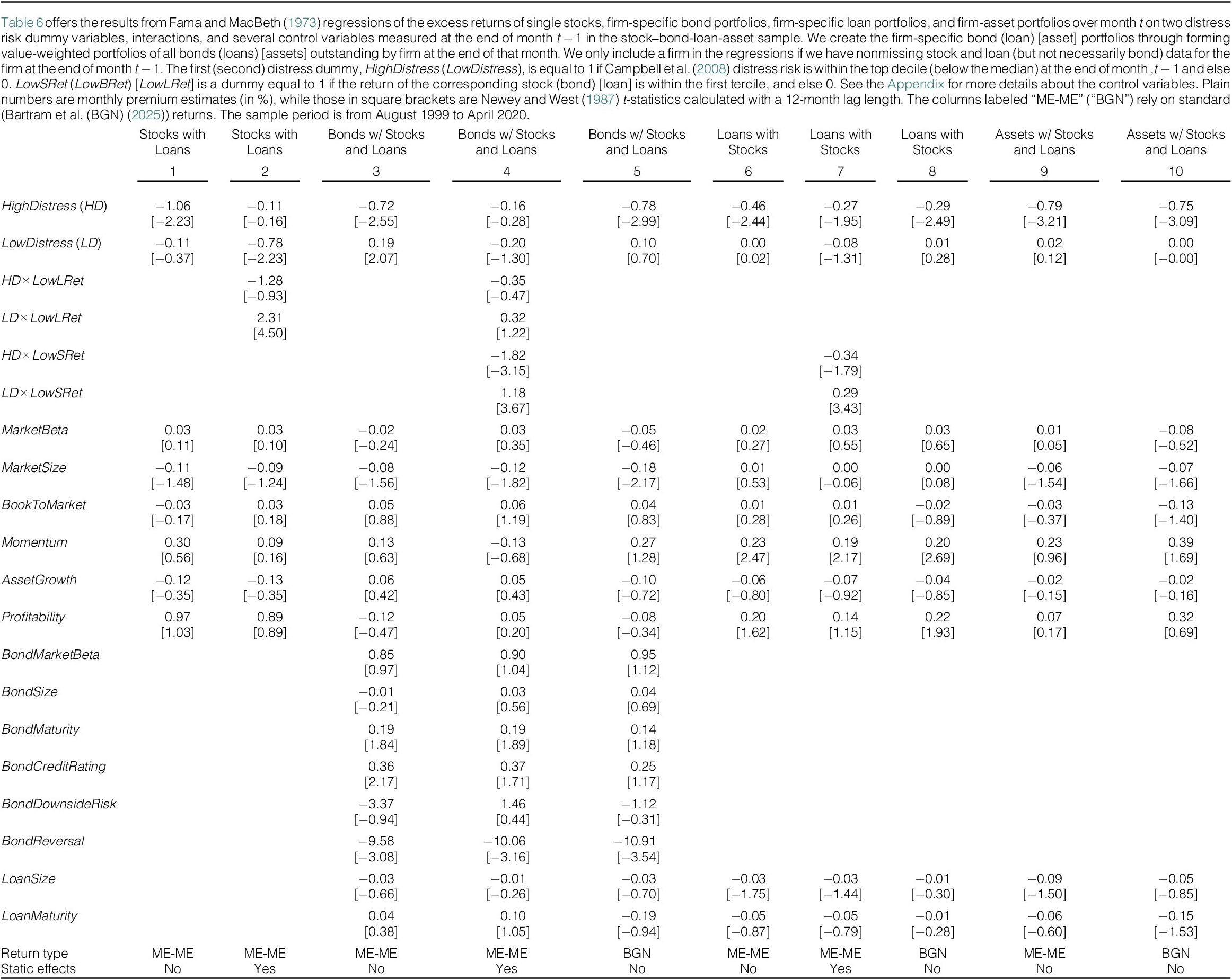
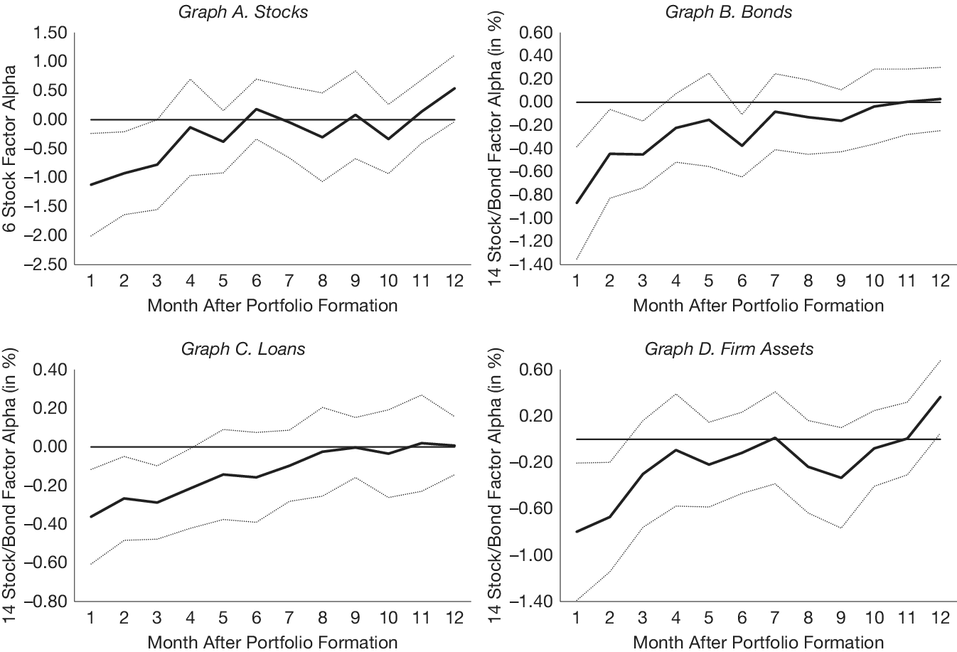
Figure 3 and Table IA.8 in the Supplementary Material study the persistence of the stock, bond, loan, and firm-asset distress premiums in the stock-bond-loan-asset sample. In particular, the figure plots the monthly FF6S stock (Graph A), SB14 bond (Graph B), SB14 loan (Graph C), and SB17 firm-asset (Graph D) alphas of the value-weighted distress quintile spread portfolios plus their corresponding 95% confidence bands separately for months $ t $
to
$ t $
to $ t+11 $
. The table offers the same results plus those from the equivalent equal-weighted portfolios and FM regressions. Both reveal that the stock and firm-asset premiums remain significant for about 2–3 months, the bond premium for about 1–4 months, and the loan premium for about 3–4 months. The weaker persistence in the stock-bond-loan-asset sample is likely due to its skew toward larger firms known to produce weaker anomalies (Fama and French (Reference Fama and French2008)).
$ t+11 $
. The table offers the same results plus those from the equivalent equal-weighted portfolios and FM regressions. Both reveal that the stock and firm-asset premiums remain significant for about 2–3 months, the bond premium for about 1–4 months, and the loan premium for about 3–4 months. The weaker persistence in the stock-bond-loan-asset sample is likely due to its skew toward larger firms known to produce weaker anomalies (Fama and French (Reference Fama and French2008)).
Figure 3 plots the monthly FF6S stock (Graph A), SB14 bond (Graph B), SB14 loan (Graph C), and SB17 firm-asset (Graph D) alpha of the value-weighted high-minus-low distress quintile spread portfolio (sold line) and the corresponding 95% confidence bands (broken lines) separately for each of the first 12 months after portfolio formation (i.e., months $ t $
to
$ t $
to $ t+11 $
) in the stock–bond-loan-asset sample.
$ t+11 $
) in the stock–bond-loan-asset sample.
D. Robustness Tests
In this section, we briefly summarize the results from several robustness tests, offering more details plus the corresponding tables and figures in the Supplementary Material.
1. The Effects of Matrix Prices
A concern about our empirical work could be that our bond sample features returns computed from Lehman Brothers, Datastream, and ICE matrix prices, which may be stale and of a notoriously poor quality. To mitigate that concern, we repeat all portfolio sorts and FM regressions exclusively using bond transaction prices from TRACE over the TRACE sample period from July 2002 to December 2020. Doing so, we also examine whether our conclusions continue to hold over a more recent sample period. Tables IA.9–IA.12 in the Supplementary Material suggest that matrix prices and our sample period do not materially affect our conclusions.
2. The Effects of Illiquidity and Liquidity Risk
Another concern could be that we do not control for bond illiquidity and liquidity risk in our main tests, especially since these variables are known to price bonds (see Bao et al. (Reference Bao, Pan and Wang2011) and Lin et al. (Reference Lin, Wang and Wu2011)) and plausibly correlated with distress risk. Our main reason for not doing so is that we require daily bond data to compute the popular proxies for these variables advocated in the two studies. Relying on daily TRACE transaction prices to compute the proxies, Tables IA.9–IA.12 in the Supplementary Material show that our portfolio sort and FM regression results are robust to controlling for them over the TRACE sample period.
3. The Effects of Changes in Bond or Loan Ownership After M&A Deals
Yet another concern may be that we rely on mappings linking our sample bonds and loans to firms not capturing changes of bond or loan ownership triggered by M&A deals. In particular, our bond mapping uses the company ticker as main firm identifier but only keeps the bond-firm link with the longest duration to mitigate the effects of nonsynchronicities in the updating of tickers in the bond and firm data.Footnote 20 Conversely, the loan mapping matches loans and firms only on the loan origination date. To address these issues, we follow Choi (Reference Choi2013) and Choi and Richardson (Reference Choi and Richardson2016) in using the CRSP event file to identify the acquirors and targets in all M&A deals (excluding asset acquisitions) from start-1986 plus the corresponding M&A dates. We next reassign the bonds and loans of targets to their acquirors if those instruments continue to be traded for at least a year after the deal date. Tables IA.13–IA.16 in the Supplementary Material show that this modification does not materially alter our conclusions.
4. The Effects of Non-Traded or Underrepresented Liabilities
A final concern could be that equation (3) is a poor approximation of true asset returns, possibly due to it omitting important non-traded liabilities or it abstracting from the non-traded loans held by even those firms with traded loans. In Tables IA.17 and IA.18 and Figure IA.5 in the Supplementary Material, we use Compustat and Capital IQ data to look deeper into that concern, evaluating the financing structure of our sample firms. Noticing that trade credit is the only important non-traded liability, we rely on arguments in Erens and Hoffmann (Reference Erens and Hoffmann2013) and Costello (Reference Costello2019) suggesting that trade credit is plausibly risk-free to include it in our asset returns. We also use Capital IQ or Mergent FISD/Compustat data to adjust the loan weight in those returns. Tables IA.19 and IA.20 in the Supplementary Material show that adjusting for trade credit and/or non-traded loans does not materially change our conclusions.
Taken together, this section shows that distress risk is not only hump-shaped or negatively related to stock-and-bond but also loan and firm-asset returns. Interestingly, however, the tendency of distressed firms to underperform is positively correlated across asset classes. The upshot is that our evidence does not suggest that redistribution effects between classes explain the distress anomaly, as, for example, posited by the shareholder advantage theory.
IV. A Disinvestment Rationale for the Distress Anomaly
In this section, we offer an explanation for the jointly negative distress premiums in stocks, bonds, loans, and firm assets in Section III. We first outline the main premise of our explanation. We next develop a real options model of a stock-and-debt financed firm making capacity utilization, investment, and disinvestment decisions. We finally reveal that the model can produce i) a negative stock (debt) distress premium if disinvestment proceeds are high and a sufficient fraction of those flow to stock (debt) claimants and ii) jointly negative premiums if those proceeds are high and debt claimants reap the lion’s share but not all of them.Footnote 21
A. The Main Premise of Our Disinvestment Rationale
Our explanation starts from noting that distressed firms often sell their real assets (see Ofek (Reference Ofek1993), Asquith, Gertner, and Scharfstein (Reference Asquith, Gertner and Scharfstein1994), and Brown, James, and Mooradian (Reference Brown, James and Mooradian1994)). Yet, as the ability to sell a real asset is akin to an American put option, and since puts have negative expected excess returns (Coval and Shumway (Reference Coval and Shumway2001)), such options lower the firm’s expected asset return, especially in distress (see Hackbarth and Johnson (Reference Hackbarth and Johnson2015) and Aretz and Pope (Reference Aretz and Pope2018)). Our contribution is to show that those options are also able to lower the firm’s expected stock or debt return in distress if a sufficient amount of disinvestment proceeds flows to the appropriate claimants.
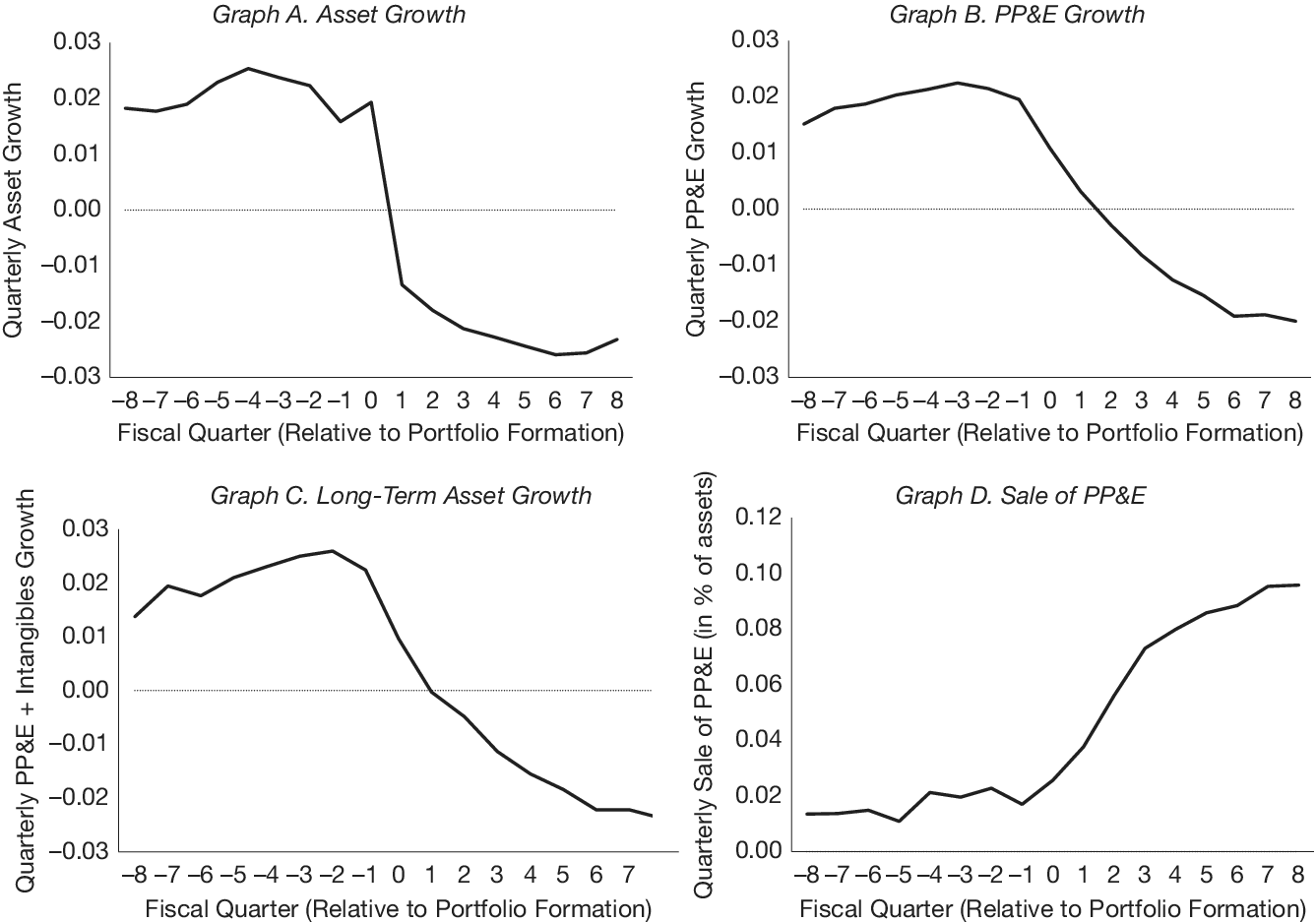
Figure 4 corroborates that our sample distressed firms also sell off their real assets. To create the figure, we select only the top-distress-decile firms from the stock–bond sample in Section IV.B and compute their quarterly asset (Graph A), property, plant, and equipment (PP&E; Graph B), and long-term asset (Graph C) growth and their sales of PP&E (Graph D) for the 16 quarters surrounding the portfolio-formation-month quarter (see the figure caption for variable definitions). To adjust for industry heterogeneity, we demean at the 49 Fama–French industry classification-quarter level. We finally take cross-sectional and then time-series averages. The figure reveals that our stock–bond sample distressed firms start selling off their real assets starting from about the portfolio formation quarter (i.e., quarter 0).
Figure 4 plots the mean asset (Graph A), net property, plant, and equipment (Graph B), and net property, plant, and equipment plus long-term intangibles (Graph C) growth and the mean proceeds from sales of property, plant, and equipment scaled by assets (Graph D) of the top-distress-decile firms in our stock–bond portfolio sort over the 16 quarters surrounding the quarter containing the portfolio formation date. We first average by cross section and then over our sample period. We use Kenneth French’s 49 industry scheme to adjust for industry heterogeneity.
B. A Real Options Model of a Stock-and-Debt Financed Firm
We study a stock-and-debt financed firm operating in continuous time $ t\in \left[0,\infty \right) $
. The firm owns a continuum of incremental options to produce a unique output good (“assets-in-place”) and options to install more of those incremental options (“growth options”). Starting with the firm’s production choices, let us index the incremental options by
$ t\in \left[0,\infty \right) $
. The firm owns a continuum of incremental options to produce a unique output good (“assets-in-place”) and options to install more of those incremental options (“growth options”). Starting with the firm’s production choices, let us index the incremental options by $ k\in \left[0,\infty \right) $
, with the kth option written on the kth output increment, and assume that the firm owns the options to produce up to the Kth output increment (so
$ k\in \left[0,\infty \right) $
, with the kth option written on the kth output increment, and assume that the firm owns the options to produce up to the Kth output increment (so $ K $
is the firm’s installed capacity). In each instant, the firm can switch on or off each option to produce, where switching on or off is cost-free. When switched on, the kth option produces one output increment per time unit at a unit cost of
$ K $
is the firm’s installed capacity). In each instant, the firm can switch on or off each option to produce, where switching on or off is cost-free. When switched on, the kth option produces one output increment per time unit at a unit cost of $ C(k)={c}_1+{c}_2k+f $
, where
$ C(k)={c}_1+{c}_2k+f $
, where $ {c}_1 $
and
$ {c}_1 $
and $ {c}_2 $
are the variable cost parameters and
$ {c}_2 $
are the variable cost parameters and $ f $
is the fixed cost parameter. When switched off, it does not produce output but still incurs a unit cost of
$ f $
is the fixed cost parameter. When switched off, it does not produce output but still incurs a unit cost of $ C(k)=f $
. We finally assume that the firm instantaneously sells its output at the stochastic price
$ C(k)=f $
. We finally assume that the firm instantaneously sells its output at the stochastic price $ \theta $
, which is governed by the geometric Brownian motion (GBM):
$ \theta $
, which is governed by the geometric Brownian motion (GBM):
 $$ d\theta =\left(\mu -\delta \right)\theta d t+\sigma \theta dW, $$
where $ \mu $
is the total expected return,
$ \mu $
is the total expected return, $ \delta $
is the dividend yield, and
$ \delta $
is the dividend yield, and $ \sigma $
is the volatility of a mimicking portfolio tracking variations in the output price, and
$ \sigma $
is the volatility of a mimicking portfolio tracking variations in the output price, and $ W $
is a Brownian motion.
$ W $
is a Brownian motion.
Our assumptions imply that the firm optimally switches on the option to produce the kth output increment in the current instant if $ \theta \ge {c}_1+{c}_2k $
. In turn, it sets its output quantity,
$ \theta \ge {c}_1+{c}_2k $
. In turn, it sets its output quantity, $ Q $
, to
$ Q $
, to $ \min \left({Q}^{\ast },K\right) $
, where
$ \min \left({Q}^{\ast },K\right) $
, where $ {Q}^{\ast } $
is the optimal quantity to produce if the firm’s installed capacity were infinite. Given
$ {Q}^{\ast } $
is the optimal quantity to produce if the firm’s installed capacity were infinite. Given $ Q $
, the firm’s profits per time unit,
$ Q $
, the firm’s profits per time unit, $ \Pi $
, are equal to
$ \Pi $
, are equal to
 $$ \Pi ={\int}_0^Q\left(\theta -{c}_1-{c}_2k\right) dk- fK=\theta Q-{c}_1Q-\frac{1}{2}{c}_2{Q}^2- fK, $$
and the firm immediately distributes those profits to its shareholders.
We next consider the capacity choices (i.e., investment and disinvestment options) of the firm. In each instant, the firm can spend the one-unit cost $ I $
to transform the growth option on the kth output increment into the corresponding option to produce. Conversely, it can sell off the option to produce that same increment, cashing in the one-unit disinvestment proceeds
$ I $
to transform the growth option on the kth output increment into the corresponding option to produce. Conversely, it can sell off the option to produce that same increment, cashing in the one-unit disinvestment proceeds $ S $
. For simplicity, we assume that, upon disinvesting an option to produce, the firm cannot reinstall it in the future, so disinvesting does not lead to reacquiring the corresponding growth option. Crucially, while the firm funds investments through raising equity, it instantaneously distributes the share
$ S $
. For simplicity, we assume that, upon disinvesting an option to produce, the firm cannot reinstall it in the future, so disinvesting does not lead to reacquiring the corresponding growth option. Crucially, while the firm funds investments through raising equity, it instantaneously distributes the share $ q $
of disinvestment proceeds to its shareholders but keeps the residual in a savings account (earning the risk-free rate) to help it honor its debt obligations. The logic is that the firm’s assets consist of easy-to-verify secured assets and hard-to-verify unsecured assets. While the firm must use the sales proceeds from secured assets to pay its debt, it can divert a share of the sales proceeds from unsecured assets to shareholders.
$ q $
of disinvestment proceeds to its shareholders but keeps the residual in a savings account (earning the risk-free rate) to help it honor its debt obligations. The logic is that the firm’s assets consist of easy-to-verify secured assets and hard-to-verify unsecured assets. While the firm must use the sales proceeds from secured assets to pay its debt, it can divert a share of the sales proceeds from unsecured assets to shareholders.
We finally discuss our capital structure assumptions. The firm is financed by common stock and a Merton (Reference Merton1974) zero-coupon bond. The bond obliges the firm to pay $ C $
at time
$ C $
at time $ T $
. Since the firm instantaneously pays profits to shareholders, it must pay its debt out of its remaining assets-in-place plus its saved disinvestment proceeds. If the firm cannot do so, it defaults, and debtholders receive the entire remaining firm value and saved disinvestment proceeds.
$ T $
. Since the firm instantaneously pays profits to shareholders, it must pay its debt out of its remaining assets-in-place plus its saved disinvestment proceeds. If the firm cannot do so, it defaults, and debtholders receive the entire remaining firm value and saved disinvestment proceeds.
C. The Real Options Model Solution
We use standard contingent claims techniques to determine the values of the firm’s assets-in-place and growth options (see Dixit and Pindyck (Reference Dixit and Pindyck1994)). Specifically, the Supplementary Material shows that the value of the option to produce the $ {k}^{th} $
output increment,
$ {k}^{th} $
output increment, $ \Delta V\left(\theta; k\right) $
, is
$ \Delta V\left(\theta; k\right) $
, is
 $$ \Delta V\left(\theta; k\right)=\left\{\begin{array}{ll}{B}_O{\theta}^{\beta_2}+\frac{\theta }{\delta }-\frac{c_1+{c}_2k+f}{r}& \hskip1.12em \mathrm{if}\;\theta \ge {c}_1+{c}_2k,\\ {}{A}_I{\theta}^{\beta_1}+{B}_I{\theta}^{\beta_2}-\frac{f}{r}& \hskip1.12em \mathrm{if}\;{\theta}^D\le \theta <{c}_1+{c}_2k,\\ {}S& \hskip1.12em \mathrm{if}\;{\theta}^D>\theta, \end{array}\right. $$
where $ r $
is the risk-free rate, and
$ r $
is the risk-free rate, and $ {B}_O $
,
$ {B}_O $
, $ {A}_I $
,
$ {A}_I $
, $ {B}_I $
,
$ {B}_I $
, $ {\theta}^D $
,
$ {\theta}^D $
, $ {\beta}_1 $
, and
$ {\beta}_1 $
, and $ {\beta}_2 $
are free parameters defined in the Supplementary Material. Intuitively,
$ {\beta}_2 $
are free parameters defined in the Supplementary Material. Intuitively, $ {B}_O $
(
$ {B}_O $
( $ {A}_I $
) [
$ {A}_I $
) [ $ {B}_I $
] determines the value of the real option to switch off (switch on) [sell off] the option to produce, and
$ {B}_I $
] determines the value of the real option to switch off (switch on) [sell off] the option to produce, and $ {\theta}^D $
is the optimal disinvestment threshold (i.e., the price at or below which the firm optimally sells the option).Footnote
22
$ {\theta}^D $
is the optimal disinvestment threshold (i.e., the price at or below which the firm optimally sells the option).Footnote
22
Conversely, the value of the corresponding growth option, $ \Delta G\left(\theta; k\right) $
, is
$ \Delta G\left(\theta; k\right) $
, is
 $$ \Delta G\left(\theta; k\right)=\left\{\begin{array}{ll}\Delta V\left(\theta; k\right)-I& \hskip1em \mathrm{if}\;\theta \ge {\theta}^{\ast },\\ {}G{\left({\theta}^{\ast}\right)}^{\beta_1}& \hskip1em \mathrm{if}\;\theta <{\theta}^{\ast },\end{array}\right. $$
where $ G $
and
$ G $
and $ {\theta}^{\ast } $
are new free parameters defined in the Supplementary Material. Intuitively,
$ {\theta}^{\ast } $
are new free parameters defined in the Supplementary Material. Intuitively, $ G $
determines the pre-exercise growth option value, and
$ G $
determines the pre-exercise growth option value, and $ {\theta}^{\ast } $
is the optimal investment threshold (i.e., the price threshold at or above which the firm optimally exercises the option).
$ {\theta}^{\ast } $
is the optimal investment threshold (i.e., the price threshold at or above which the firm optimally exercises the option).
We can finally compute the total value of the firm, $ V\left(\theta \right) $
, from
$ V\left(\theta \right) $
, from
 $$ V\left(\theta \right)={\int}_0^K\Delta V\left(\theta; k\right) dk+{\int}_K^{\infty}\Delta G\left(\theta; k\right) dk, $$
which we numerically approximate through the trapezoidal method.
Unfortunately, it is impossible to determine the values of the common stock and the zero-coupon bond in closed-form. As a result, we use a Monte Carlo simulation technique to obtain them. To do so, we write the value of the zero-coupon bond, $ D\left(\theta; T\right) $
, as
$ D\left(\theta; T\right) $
, as
 $$ D\left(\theta; T\right)={E}^{\unicode{x211A}}\left[{e}^{- rT}\min \Big(C,V\left({\theta}_T\right)+\left(1-q\right){S}_T\Big)\right], $$
where $ {E}^{\unicode{x211A}} $
is the expectation operator under the equivalent martingale measure,
$ {E}^{\unicode{x211A}} $
is the expectation operator under the equivalent martingale measure, $ V\left({\theta}_T\right) $
is the value of the firm’s assets-in-place and growth options at time
$ V\left({\theta}_T\right) $
is the value of the firm’s assets-in-place and growth options at time $ T $
, and
$ T $
, and $ {S}_T $
is the compounded-up value of the disinvestment proceeds collected by the firm until that same time. We then simulate 100,000 sample paths for the daily output price
$ {S}_T $
is the compounded-up value of the disinvestment proceeds collected by the firm until that same time. We then simulate 100,000 sample paths for the daily output price $ \theta $
from time
$ \theta $
from time $ t=0 $
to
$ t=0 $
to $ T $
under the equivalent martingale measure, derive the firm’s optimal capacity utilization, investment, and disinvestment choices at the end of each day, and calculate
$ T $
under the equivalent martingale measure, derive the firm’s optimal capacity utilization, investment, and disinvestment choices at the end of each day, and calculate $ {e}^{- rT}\min \left(C,V\left({\theta}_T\right)+\left(1-q\right){S}_T\right) $
for each path. Averaging over the 100,000
$ {e}^{- rT}\min \left(C,V\left({\theta}_T\right)+\left(1-q\right){S}_T\right) $
for each path. Averaging over the 100,000 $ {e}^{- rT}\min \left(C,V\left({\theta}_T\right)+\left(1-q\right){S}_T\right) $
values, we obtain
$ {e}^{- rT}\min \left(C,V\left({\theta}_T\right)+\left(1-q\right){S}_T\right) $
values, we obtain $ D\left(\theta; T\right) $
. Subtracting
$ D\left(\theta; T\right) $
. Subtracting $ D\left(\theta; T\right) $
from
$ D\left(\theta; T\right) $
from $ V\left(\theta \right) $
, the initial firm value, we obtain the value of the common stock,
$ V\left(\theta \right) $
, the initial firm value, we obtain the value of the common stock, $ E\left(\theta; T\right) $
. See the Supplementary Material for more technical details.
$ E\left(\theta; T\right) $
. See the Supplementary Material for more technical details.
We follow Cox and Rubinstein (Reference Cox and Rubinstein1985) in computing the instantaneous expected excess return of the assets ( $ X=V $
), debt (
$ X=V $
), debt ( $ X=D $
), or stocks (
$ X=D $
), or stocks ( $ X=E $
),
$ X=E $
), $ E\left[{R}_X^{ie}\right] $
, from
$ E\left[{R}_X^{ie}\right] $
, from
 $$ {\displaystyle \begin{array}{c}E\left[{R}_X^{ie}\right] dt=E\left[ dX/X\right]+\pi / Xdt- rdt=E\left[ dX/X\right]+\pi / Xdt\\ {}-\left({E}^{\unicode{x211A}}\left[ dX/X\right]+\pi / Xdt\right)\\ {}=\left(\left(\mu -\delta \right)\theta {X}_{\theta }+\frac{1}{2}{\sigma}^2{\theta}^2{X}_{\theta \theta}+{X}_t\right)/ Xdt\\ {}-\left(\left(r-\delta \right)\theta {X}_{\theta }+\frac{1}{2}{\sigma}^2{\theta}^2{X}_{\theta \theta}+{X}_t\right)/ Xdt\\ {}={X}_{\theta}\left(\theta /X\right)\left(\mu -r\right) dt,\end{array}} $$
where $ \pi $
is the claim’s payoff,
$ \pi $
is the claim’s payoff, $ {X}_{\theta } $
and
$ {X}_{\theta } $
and $ {X}_t $
the first partial derivatives of the claim’s value with respect to the output price
$ {X}_t $
the first partial derivatives of the claim’s value with respect to the output price $ \theta $
and time
$ \theta $
and time $ t $
, respectively, and
$ t $
, respectively, and $ {X}_{\theta \theta} $
the second partial derivative of that value with respect to the output price. We rely on Itô’s lemma to derive the differential
$ {X}_{\theta \theta} $
the second partial derivative of that value with respect to the output price. We rely on Itô’s lemma to derive the differential $ dX $
. Intuitively, equation (11) suggests that a claim’s expected excess return is linear in its elasticity, defined as its delta,
$ dX $
. Intuitively, equation (11) suggests that a claim’s expected excess return is linear in its elasticity, defined as its delta, $ {X}_{\theta } $
, times the claim value-to-output price ratio,
$ {X}_{\theta } $
, times the claim value-to-output price ratio, $ \theta /X $
.
$ \theta /X $
.
D. The Effect of Real Disinvestments on the Distress Premium
We now investigate the real-options-model-implied effect of distress risk on the expected asset, stock, and debt return of the firm. In the base case, we set the firm’s initial capacity, $ K $
, to one. We further rely on an annualized total expected return,
$ K $
, to one. We further rely on an annualized total expected return, $ \mu $
, dividend yield,
$ \mu $
, dividend yield, $ \delta $
, and volatility,
$ \delta $
, and volatility, $ \sigma $
, of the output-price mimicking portfolio of 12%, 8%, and 45%, respectively, and a risk-free rate,
$ \sigma $
, of the output-price mimicking portfolio of 12%, 8%, and 45%, respectively, and a risk-free rate, $ r $
, of 4%. We select the variable production cost parameters,
$ r $
, of 4%. We select the variable production cost parameters, $ {c}_1 $
and
$ {c}_1 $
and $ {c}_2 $
, to be 0.00 and 0.30, respectively, and the fixed production cost parameter,
$ {c}_2 $
, to be 0.00 and 0.30, respectively, and the fixed production cost parameter, $ f $
, to be 0.70. We choose a bond repayment,
$ f $
, to be 0.70. We choose a bond repayment, $ C $
, and time-to-maturity,
$ C $
, and time-to-maturity, $ T $
, of 10.00 and 2.00, respectively. Consistent with distressed firms owning few valuable growth opportunities, we select an investment cost,
$ T $
, of 10.00 and 2.00, respectively. Consistent with distressed firms owning few valuable growth opportunities, we select an investment cost, $ I $
, of 100, ensuring that growth options make up an only small portion of total value.
$ I $
, of 100, ensuring that growth options make up an only small portion of total value.
We first study the effect of distress risk on the expected asset return separately for firms varying in the ease with which they can sell their assets-in-place. To do so, we always let the initial output price, $ \theta $
, range from the lowest value at which the firm does not immediately disinvest some capacity to 2.00. To vary the firm’s ability to disinvest, we set the disinvestment proceeds,
$ \theta $
, range from the lowest value at which the firm does not immediately disinvest some capacity to 2.00. To vary the firm’s ability to disinvest, we set the disinvestment proceeds, $ S $
, to 0.00, 4.00, or 8.00. In Figure 5, we then plot the expected excess asset return (equation (11)) against distress risk (the probability that
$ S $
, to 0.00, 4.00, or 8.00. In Figure 5, we then plot the expected excess asset return (equation (11)) against distress risk (the probability that $ V\left({\theta}_T\right)+\left(1-q\right){S}_T<C $
) for each
$ V\left({\theta}_T\right)+\left(1-q\right){S}_T<C $
) for each $ S $
value. The figure suggests that a greater ability to disinvest (i.e., a higher
$ S $
value. The figure suggests that a greater ability to disinvest (i.e., a higher $ S $
value) lowers the expected asset returns especially for distressed firms. Specifically, while the expected asset returns of low-distress-risk firms are close to one another, those returns vividly rise (fall) with distress risk under a low (high)-disinvestment ability. The reason is that distressed firms without valuable disinvestment options have high operating leverage boosting their systematic risk (see Carlson, Fisher, and Giammarino (Reference Carlson, Fisher and Giammarino2004) and Cooper (Reference Cooper2006)). Yet, when distressed firms possess such options, the options’ negative risk can dominate the positive operating leverage risk, lowering the firms’ expected returns (see Hackbarth and Johnson (Reference Hackbarth and Johnson2015) and Aretz and Pope (Reference Aretz and Pope2018)).
$ S $
value) lowers the expected asset returns especially for distressed firms. Specifically, while the expected asset returns of low-distress-risk firms are close to one another, those returns vividly rise (fall) with distress risk under a low (high)-disinvestment ability. The reason is that distressed firms without valuable disinvestment options have high operating leverage boosting their systematic risk (see Carlson, Fisher, and Giammarino (Reference Carlson, Fisher and Giammarino2004) and Cooper (Reference Cooper2006)). Yet, when distressed firms possess such options, the options’ negative risk can dominate the positive operating leverage risk, lowering the firms’ expected returns (see Hackbarth and Johnson (Reference Hackbarth and Johnson2015) and Aretz and Pope (Reference Aretz and Pope2018)).
Figure 5 plots the expected excess asset return against default risk separately for a disinvestment gain, $ S $
, of 0, 4, and 8. See Section IV.D for more details about our basecase parameter value choices.
$ S $
, of 0, 4, and 8. See Section IV.D for more details about our basecase parameter value choices.
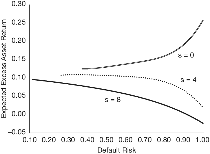
Notwithstanding, the more critical question for our purposes is whether a high-disinvestment ability can also induce expected stock or debt returns to fall with distress risk. To tackle that question, Figure 6 plots the expected excess stock (Graph A) and debt (Graph B) return against distress risk under disinvestment proceeds, $ S $
, of 8.00 and a share of proceeds going to shareholders,
$ S $
, of 8.00 and a share of proceeds going to shareholders, $ q $
, of 0.00, 0.05, 0.10, and 0.25. The figure suggests that the model can yield a negative (or, more accurately, negatively hump-shaped) relation between distress risk and expected stock (debt) returns if a sufficient amount of disinvestment proceeds flow to stock (debt) claimants. In particular, the stock (debt) relation becomes negative if at least 5% (75%) of proceeds flow to stock (debt) claimants. Strikingly, the figure also shows that the model can produce a jointly negative relation for stocks and debt if the lion’s share of proceeds flows to debtholders (e.g., 90%) but a small residual to shareholders (e.g., 10%).Footnote
23
$ q $
, of 0.00, 0.05, 0.10, and 0.25. The figure suggests that the model can yield a negative (or, more accurately, negatively hump-shaped) relation between distress risk and expected stock (debt) returns if a sufficient amount of disinvestment proceeds flow to stock (debt) claimants. In particular, the stock (debt) relation becomes negative if at least 5% (75%) of proceeds flow to stock (debt) claimants. Strikingly, the figure also shows that the model can produce a jointly negative relation for stocks and debt if the lion’s share of proceeds flows to debtholders (e.g., 90%) but a small residual to shareholders (e.g., 10%).Footnote
23
Figure 6 plots the expected excess stock (Graph A) and debt (Graph B) return against default risk assuming a disinvestment gain, $ S $
, of 8 and separately for a fraction of disinvestment proceeds distributed to shareholders,
$ S $
, of 8 and separately for a fraction of disinvestment proceeds distributed to shareholders, $ q $
, equal to 0, 0.05, 0.10, and 0.25. See Section IV.D for details about the basecase parameter values.
$ q $
, equal to 0, 0.05, 0.10, and 0.25. See Section IV.D for details about the basecase parameter values.
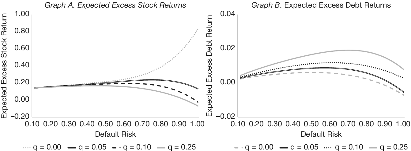
All in all, this section shows that, in a real options model of a stock-and-debt financed firm with capacity utilization, investment, and disinvestment choices, the ability to disinvest real assets can not only switch the distress risk-expected asset return relation from positive to negative but also the stock and debt relations—if a sufficient amount of disinvestment proceeds flows to the appropriate claimants. More importantly, such a model can yield jointly negative relations if the lion’s share but not all of the proceeds flows to debtholders.
V. Empirical Tests of our Disinvestment Rationale
In this section, we empirically test the new implications of our real options model for the distress anomaly in Section IV. We first describe the variables used to proxy for the ease with which firms can disinvest their hard assets. We next offer the results from FM regressions of stock, bond, and loan returns on distress risk and controls separately estimated on firms with easier and harder-to-disinvest assets. We finally condition the regressions on volatility.
A. The Disinvestment Ability Proxies
We use as proxies for the ease with which a firm can disinvest its hard assets: i) Gu et al.’s (Reference Gu, Hackbarth and Johnson2018) asset inflexibility, ii) Eisfeldt and Rampini’s (Reference Eisfeldt and Rampini2006) asset reallocation, iii) Schlingemann et al.’s (Reference Schlingemann, Stulz and Walkling2002) asset liquidity, and iv) Bai et al.’s (Reference Bai, Li, Xue and Zhang2025) investment skewness.Footnote 24 We calculate asset inflexibility as the range of the quarterly operating costs-to-quarterly sales ratio scaled by the volatility of the log change in the sales-to-assets ratio of a firm’s industry, where operating costs are costs of goods sold plus selling, general, and administrative costs. Asset reallocation is a firm’s annual acquisition expenses plus sales of property, plant, and equipment scaled by assets. Asset liquidity is the number of asset acquisition, firm acquisition, and merger deals in a firm’s industry over the last year. Finally, investment skewness is the sample skewness of the annual growth in the sum of net property, plant, and equipment plus depreciation and amortization of a firm’s industry. See the Appendix for more details.
The logic behind those proxies is as follows: A higher asset inflexibility signals a lower-disinvestment ability since firms waiting longer to disinvest in response to negative shocks observe greater drops in their sales than operating costs (due to fixed operating costs). In turn, they have more variable operating costs-to-sales ratios. Conversely, a higher asset reallocation signals a greater-disinvestment ability since higher-ability firms adjust their installed capacity more rapidly in response to shocks.Footnote 25 A higher asset liquidity signals a greater-disinvestment ability since it indicates that firms’ real assets are traded in more active and liquid secondary markets. Finally, a more positive investment skewness signals a lower-disinvestment ability since the inability to disinvest truncates the investment distribution from the left.
In Table 7, we aim to validate the disinvestment ability proxies. To do so, we report the mean asset-sale-value-to-assets ratio for firms in the top (10), moderate (6–9), and low (1–5) distress deciles formed from the stock–bond sample in Section V.B separately for firms with an above third and below first quartile value for each disinvestment ability proxy. We obtain the asset-sale values from SDC Platinum. We compute the mean ratios by first averaging by portfolio formation date and then over our sample period. The table corroborates that firms classified by our proxies as high-disinvestment-ability markedly raise their asset sales in response to distress risk (see columns 1, 3, 5, and 7). For example, column 1 reveals that while low-distress and low-asset-inflexibility firms sell off about 7.41% of their assets, the corresponding number for high-distress firms is about 17.45%. In comparison, the asset sales of low-disinvestment-ability firms do not strongly relate to distress (see columns 2, 4, 6, and 8). Contrasting high-distress firms with a high- and low-disinvestment ability, the high-ability firms usually sell off more of their assets than their counterparts.
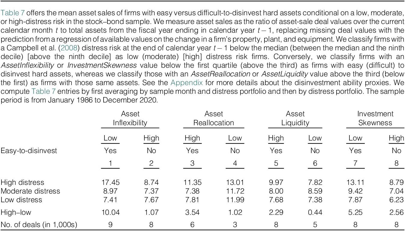
B. The Conditional Effect of Disinvestment Options
We next test whether the ability of firms to disinvest real assets helps to explain the negative stock, bond, loan, and firm-asset distress premiums in Section III. To that end, Table 8 reports the results from repeating the stock-and-bond FM regressions in columns 1, 4, and 6 of Table 3 and the loan regressions in columns 6 and 8 of Table 6 on subsamples of firms with high (above third quartile) and low (below first) values for each disinvestment ability proxy. Panels A, B, and C focus on stocks, bonds, and loans, respectively. As before, plain numbers are monthly premium estimates, while those in square brackets are Newey and West (Reference Newey and West1987) t-statistics with a 12-month lag length. To conserve space, we report estimates and t-statistics only for the distress dummy variables but not the controls.
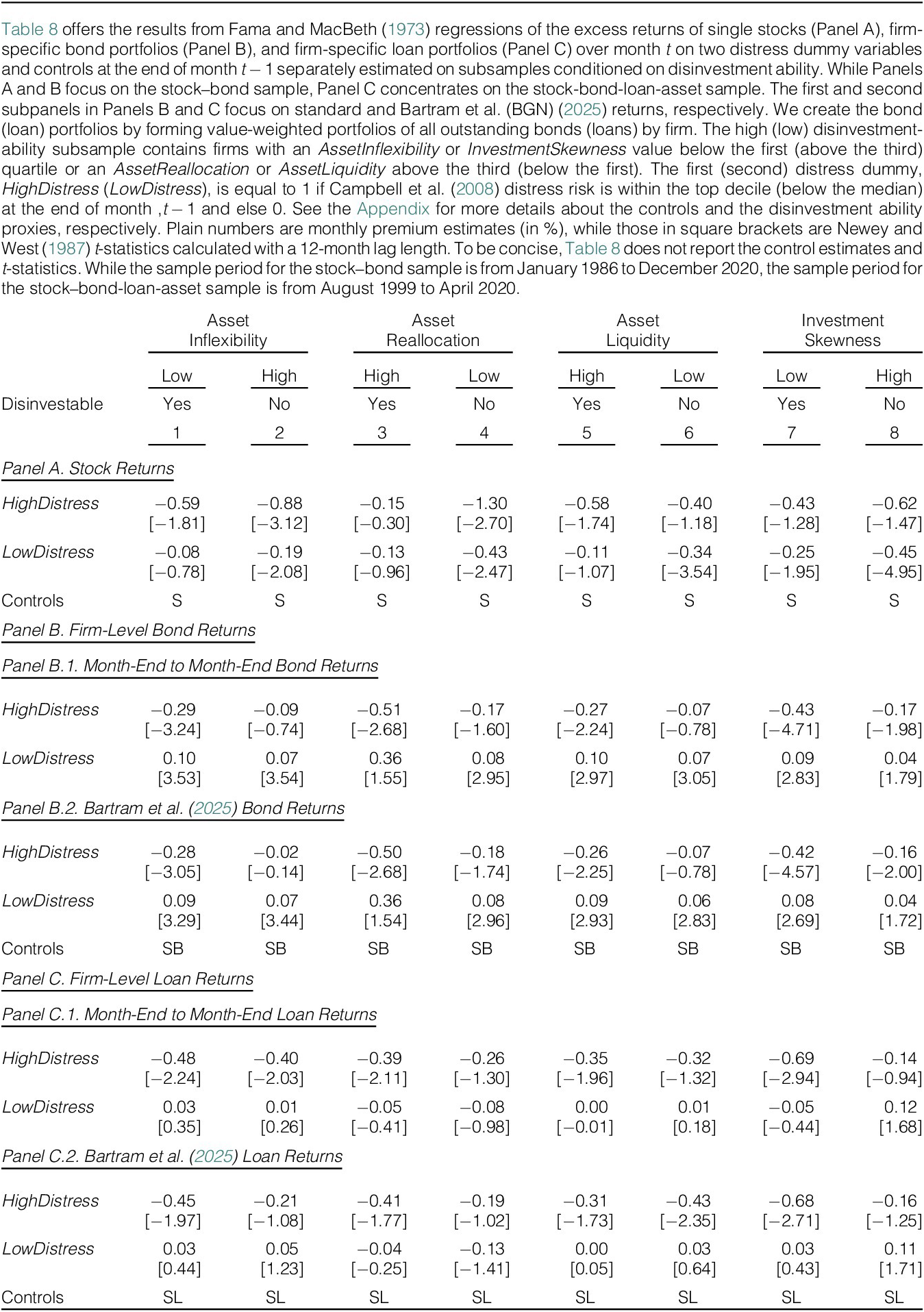
Starting off with our sample bonds and loans, Panels B and C suggest that their distress premiums are significantly more negative in the subsamples of firms with a higher-disinvestment ability, in line with firms owning easy-to-disinvest hard assets selling those in distress and distributing most of the proceeds to debtholders. Columns 1 and 2 in Panel B, for example, show that while the monthly standard-return bond distress premium is an insignificant −0.09% (t-stat: −0.74) in the high asset inflexibility (low-disinvestment ability) subsample, the corresponding number is a significant −0.29% (t-stat: −3.24) in the low inflexibility (high ability) subsample (contrast the coefficients on the HighDistress variable). As another example, columns 7 and 8 in Panel C reveal that while the standard-return loan distress premium is an insignificant −0.14% (t-stat: −0.94) in the high investment skewness (low-disinvestment ability) subsample, the corresponding number is a significant −0.69% (t-stat: −2.94) in the low skewness (high ability) subsample. Overall, the bond premium is significantly negative at the 95% level in eight (out of eight) cases in the high but in only two in the low disinvestment-ability subsample. Conversely, the loan premium is significantly negative in six cases in the high but only in two in the low disinvestment-ability subsample.
Reverting to our sample stocks, Panel A shows that their distress premium tends to be significantly more negative in the lower-disinvestment-ability subsamples. Columns 3 and 4, for example, suggest that while the monthly stock distress premium is an insignificant −0.15% (t-stat: −0.30) in the high asset reallocation (high-disinvestment ability) subsample, it is a significant −1.30% (t-stat: −2.70) in the low reallocation (low ability) subsample. Overall, the stock distress premium is significantly negative at the 95% level in two (out of four) cases in the low but in none in the high-disinvestment ability subsamples.
While it could be seen as puzzling that the ability to disinvest hard assets conditions the stock distress premium with the opposite sign compared to the bond and loan premiums, we note that easier-to-disinvest hard assets are likely attractive as collateral in debt contracts due to, for example, their high fire-sale values. As a result, it is likely that the proceeds from disinvesting them flow to debtholders, and not shareholders. In contrast, hard-to-disinvest hard assets are likely less attractive as collateral, allowing firms to channel some of the proceeds from disinvesting them to shareholders. Yet, as we demonstrate in Section IV, assigning an only small fraction of disinvestment proceeds to shareholders can already switch the distress risk-expected stock return relation from positive to negative.
C. The Conditional Effect of Volatility
We now offer further evidence that the modulating effect of the disinvestment ability proxies on the stock, bond, and loan distress premiums in Section V.B can be attributed to variations in the ease with which firms are able to sell their hard assets. To that end, we recall that the value of real options (such as the disinvestment option) rises with uncertainty. The upshot is that the modulating effect of the disinvestment ability proxies should be stronger for firms exposed to more uncertainty (see Grullon, Lyandres, and Zhdanov (Reference Grullon, Lyandres and Zhdanov2012) and our comparative statics on the effect of output-price volatility on the stock and debt distress premiums in Section IA.7.3 of the Supplementary Material). To test that conjecture, we choose those subsamples from Table 8 generating a stronger distress anomaly (i.e., the hard-to-disinvest stock and easy-to-disinvest bond and loan subsamples) and further split them according to the median of historical stock volatility. We estimate historical volatility from firm-specific regressions of the monthly stock return on the Fama and French (Reference Fama and French1993) 3-factor model factors over the last 2 years of data and computing the annualized volatility of the residual. We finally repeat the relevant regressions from Table 8 separately on the subsamples with a high versus low historical stock volatility.
Using a design similar to Table 8, Table 9 offers the subsample regression results. As always, plain numbers are monthly premium estimates, whereas those in square brackets are Newey and West (Reference Newey and West1987) t-statistics. The table supports the conjecture that the modulating effect of the disinvestment ability proxies is stronger in the higher-volatility subsamples. For example, while a high-distress risk lowers the monthly mean stock return of high-volatility, low inflexible-asset firms by a significant 0.73% (t-stat: −2.04), the corresponding change is an insignificant −0.24% (t-stat: −0.54) for low-volatility firms (contrast the HighDistress coefficient across columns 1 and 2 in Panel A). In the same vein, while a high-distress risk lowers the monthly mean standard loan return of high-volatility, high asset-liquidity firms by a significant 0.55% (t-stat: −2.29), the corresponding change is an insignificant 0.00% (t-stat: 0.03) for low-volatility firms (contrast the same coefficient across columns 5 and 6 in Panel C.1). Overall, the modulating effect of the disinvestment ability proxies is stronger in the high versus the low-volatility sample in all but two cases.
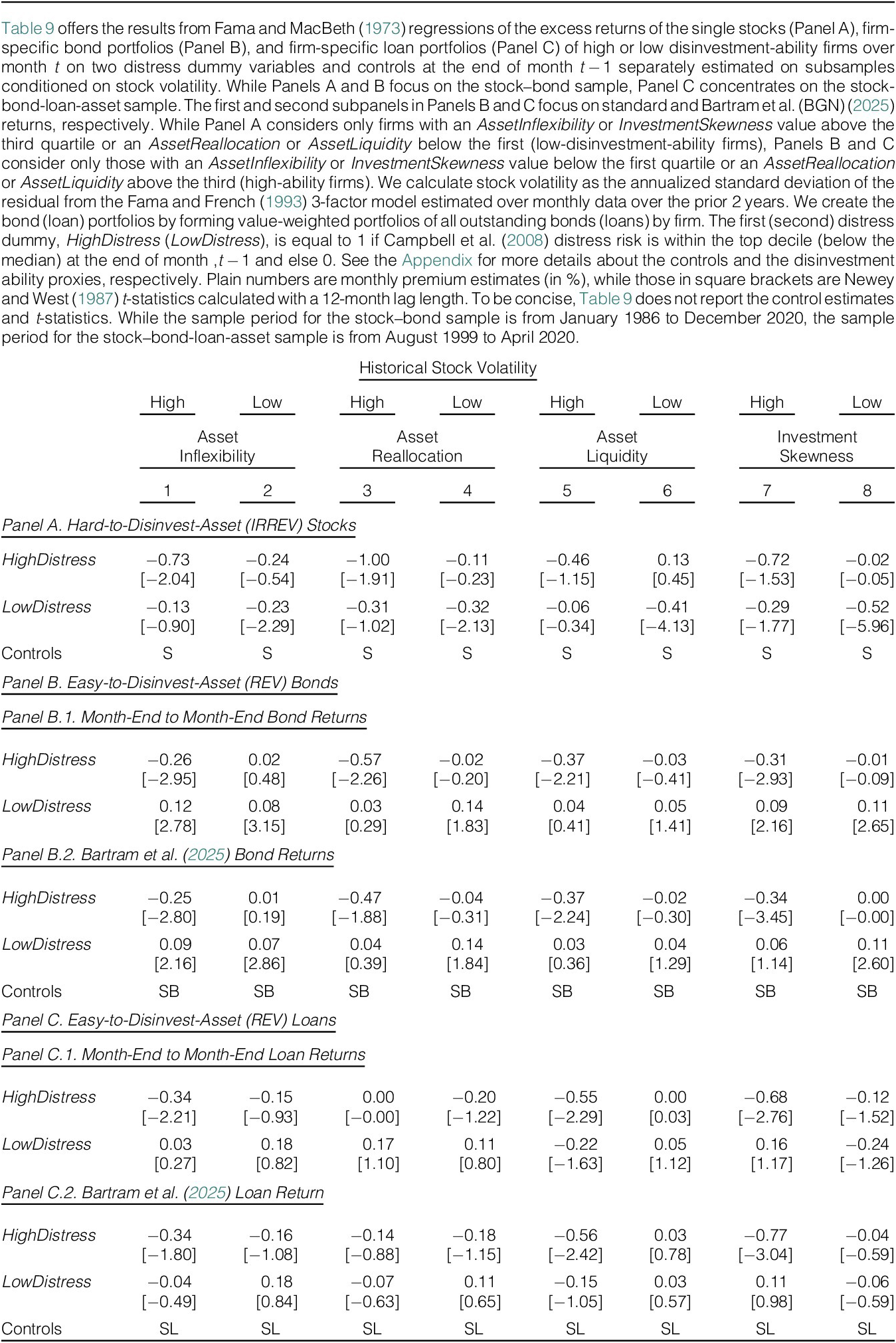
VI. Concluding Remarks
We show that, analogous to the hump-shaped stock and negative bond mean return-distress relations exposed in the literature, those same relations are also negative for traded loans and firm assets, with the same firms appearing to be behind the nonpositive relations. Spurred by the negative firm-asset relation, we speculate that the distress anomaly could be due to operational risk, such as the ability of firms to disinvest real assets in distress. We use a standard real options model of a stock-and-debt financed firm with capacity utilization, expansion, and contraction choices to back up our intuition. The model confirms that the ability to disinvest real assets can not only lower the expected asset returns of distressed firms but also their expected stock (debt) returns if a large enough amount of disinvestment proceeds flows to shareholders (debtholders). Critically, the model can produce jointly negative distress premiums if the lion’s share of disinvestment proceeds flows to debtholders but a small residual to shareholders. Using proxies for the ease with which a firm can disinvest its hard assets, we establish that while the bond and loan distress premiums become more negative with these proxies, the stock premium often becomes less negative with them, likely because easy-to-disinvest hard assets are more plausibly secured than their counterparts.
Appendix. Additional Variable-Calculation Details
In this appendix, we offer details on how we calculate i) bond returns, ii) Campbell et al.’s (Reference Campbell, Hilscher and Szilagyi2008) default risk predictors, and iii) our controls. At the end, we also offer lists summarizing the definitions of our controls and disinvestment ability proxies.
A.1. Calculating NAIC and TRACE Bond Returns
We use equation (1) to calculate bond returns from NAIC and TRACE data. To that end, we require the daily bond price, the accrued interest, and the coupon payment. We follow the literature in calculating those variables. To be specific, we compute a bond’s daily price from TRACE as a trading-volume-weighted average of its intra-day prices, minimizing confounding effects arising from the bid–ask spread. To calculate the accrued interest from TRACE, we first compute the daily coupon rate as the coupon rate divided by 360 if a bond’s day-count basis is “30/360” or “ACT/360” and as that same rate divided by the actual number of calendar days per year if it is “ACT/ACT.” We next count the calendar days between the current month-end $ t $
and the previous coupon date, assuming a number of days per calendar month equal to 30 if the day-count basis is “30/360” and equal to the actual number of days if “ACT/360” or “ACT/ACT.” We use the first coupon date and the coupon frequency to infer when coupons are paid. We finally calculate the accrued interest
$ t $
and the previous coupon date, assuming a number of days per calendar month equal to 30 if the day-count basis is “30/360” and equal to the actual number of days if “ACT/360” or “ACT/ACT.” We use the first coupon date and the coupon frequency to infer when coupons are paid. We finally calculate the accrued interest $ AI $
as the daily coupon rate times the number of days between current month-end
$ AI $
as the daily coupon rate times the number of days between current month-end $ t $
and previous coupon date.
$ t $
and previous coupon date.
We compute two alternative bond returns from NAIC and TRACE. Defining the start (end) of a month as its first (last) five trading days, the first ranges from the start of month $ t $
to the end of that month, while the second ranges from the start of month
$ t $
to the end of that month, while the second ranges from the start of month $ t $
to the start of month
$ t $
to the start of month $ t+1 $
. If there are multiple nonmissing daily prices over a five-day (start or end of month) period, we always choose that closest to the turn of the month. If we can calculate both alternatives, we always pick that from start of month
$ t+1 $
. If there are multiple nonmissing daily prices over a five-day (start or end of month) period, we always choose that closest to the turn of the month. If we can calculate both alternatives, we always pick that from start of month $ t $
to start of month
$ t $
to start of month $ t+1 $
.Footnote
26
$ t+1 $
.Footnote
26
A.2. Calculating Campbell et al.’s (Reference Campbell, Hilscher and Szilagyi2008) Default Risk Predictors
We use Campbell et al.’s (Reference Campbell, Hilscher and Szilagyi2008) hazard model to measure distress risk, projecting a dummy variable equal to 1 if a firm defaults, files for bankruptcy, or is delisted for performance reasons over the month 12 months from the current, and else 0, Failure, on distress risk predictors measured at the end of the current month (recall equation (4) in Section II.B). The distress risk predictors are NIMTA, TLMTA, CASHMTA, MB, SIGMA, EXRET, SIZE, and PRICE. NIMTA is the ratio of net income to the sum of the market value of equity and the book value of total liabilities (“market-value-adjusted total assets”). TLMTA is the ratio of the book value of total liabilities to those same assets. CASHMTA is the sum of cash and short-term assets to those assets. MB is the market-to-book ratio, where we add 10% of the difference between the market and book value of equity to the book value of equity and set book values of equity which continue to be negative to $1. EXRET is the monthly log stock return in excess of the monthly log S&P 500 return. SIGMA is a stock’s volatility obtained from daily data over the prior 3 months.Footnote 27 SIZE is the log ratio of a stock’s market capitalization to the S&P 500’s total market capitalization. Finally, PRICE is the log stock price truncated from above at $15.
To enhance the timeliness of the predictors, we follow Campbell et al. (Reference Campbell, Hilscher and Szilagyi2008) in using quarterly accounting data in our calculations, assuming that the accounting values become publicly available with a 2-month reporting gap (i.e., 2 months after the end of the fiscal quarter). To guard against outliers, we winsorize the distress risk predictors at the 5th and 95th percentiles.
A.3. Calculating Our Control Variables
Our portfolio sorts control for systematic risk by calculating the intercept (“alpha”) from a time-series regression of a portfolio’s excess return (i.e., its return minus the risk-free rate) on the factors from alternative factor models. As we said, we use the FF3S, the FF5S, and the FF6S models for our stock portfolios. Intuitively, the FF3S model contains as factors the excess stock market return (MKT) and the returns of spread portfolios formed on stock size (SMB) and the book-to-market ratio (HML). The FF5S model then adds the returns of spread portfolio formed on asset growth (CMA) and profitability (RMW). Finally, the FF6S model adds the return of a spread portfolio formed on the intermediate-term past return (MOM). See Kenneth French’s website for more details about the stock factors. We use the FF5SB, SB8, and SB14 models for our bond and loan portfolios. The FF5SB model contains the MKT, SMB, and HML stock factors plus the returns of a corporate bond spread portfolio formed on default risk (DEF) and a government bond portfolio formed on maturity time (TERM). See Amit Goyal’s website for more details about the DEF and TERM factors. The SB8 model adds the returns of a value-weighted portfolio of corporate bonds with a rating equal to or above BBB– (IGBMKT) and a value-weighted portfolio of corporate bonds with a rating below BBB– (SGBMKT) and the return of a corporate bond spread portfolio formed on the intermediate-term past return (BMOM). Finally, the SB14 model adds the returns of corporate bond spread portfolios formed on the bond book-to-market ratio (BHML), the prior-month return (BSTR), the long-term past return (BLTR), duration (BDUR), carry (BCAR), and earnings announcement drift (BPEAD). See the Open Source Bond Asset Pricing website for more details about the BMOM, BHML, BSTR, BLTR, BDUR, BCAR, and BPEAD factors. We add the CMA, RMW, and MOM stock factors to the FF5SB, SB8, and SB14 model factors to create the SB8, SB11, and SB17 models to control for the systematic risk of our firm-asset portfolios, respectively. We obtain data on all the factors of those factor models except IGBMKT and SGBMKT (which we calculate ourselves) from the cited websites.Footnote 28
Our FM regressions rely on both factor exposures and characteristics as control variables. In the stock regressions, we include a stock’s exposure to the excess stock market return (MarketBeta) and its log market size (MarketSize), book-to-market ratio (BookToMarket), past 11-month return (Momentum), asset growth (AssetGrowth), and profitability (Profitability). In the bond regressions, we add a bond’s exposure to the excess bond market return (BondMarketBeta) and its amount outstanding (BondSize), time-to-maturity (BondMaturity), most recent credit rating (BondCreditRating), 5% Value-at-Risk (BondDownsideRisk), and short-term past return (BondReversal). In contrast, the loan regressions add the loan’s market value (LoanSize) and its time-to-maturity (LoanMaturity). We estimate the exposures from rolling window regressions over the past 36 months of monthly data. We further always winsorize the factor exposures and characteristics at the 1st and 99th percentiles per sample month. See the following for details.
Below, we offer the exact definitions of all the control variables used in our regressions. We update the controls indexed by “M” on a monthly basis and use their values to condition stock, bond, loan, and firm-asset returns over the next month. We update those indexed by “A” on an annual basis and use their values to condition those same returns over the period from July of year $ t $
to June of year
$ t $
to June of year $ t+1 $
. We show the data-provider mnemonics in parentheses.
$ t+1 $
. We show the data-provider mnemonics in parentheses.
Stock Control Variables
- MarketBeta (M):
-
Slope coefficient from a time-series regression of a stock’s excess return on the value-weighted CRSP index excess return (vwretd) estimated over the prior 36 months of monthly data (see Fama and MacBeth (Reference Fama and MacBeth1973) and McLean and Pontiff (Reference McLean and Pontiff2016)).
- MarketSize (A):
-
Log stock size (abs(prc) $ \times $
shrout) at the end of June of year
$ t $
(see Fama and French (Reference Fama and French1992)).
$ \times $
shrout) at the end of June of year
$ t $
(see Fama and French (Reference Fama and French1992)). - BookToMarket (A):
-
Log of the ratio of the book value of equity to the market value of equity (abs(prc)
$ \times $
shrout), where the book value of equity is equal to total assets (at) minus total liabilities (lt) plus deferred taxes (txditc, zero if missing) minus preferred stock (pstkl, pstkrv, prfstck, or zero; in that order of availability). We take the values of all variables used in the calculation from the fiscal year end in calendar year
$ t-1 $
(see Fama and French (Reference Fama and French1992)). - Momentum (M):
-
A stock’s dollar return (ret) compounded over the prior 12 months of monthly data, but excluding the most recent month (see Jegadeesh and Titman (Reference Jegadeesh and Titman1993)).
- AssetGrowth (A):
-
Log of the gross change in total assets (at) from the fiscal year end in calendar year
$ t-2 $
to the fiscal year end in calendar year
$ t-1 $
(see Cooper, Gulen, and Schill (Reference Cooper, Gulen and Schill2008)). - Profitability (A):
-
Ratio of sales (sale) net of costs of goods sold (cogs), selling, general, and administrative expenses (xsge), and interest expenses (xint) to the book value of equity, where the book value of equity is total assets (at) less total liabilities (lt) plus deferred taxes (txditc, zero if missing) less preferred stock (pstkl, pstkrv, prfstck, or zero; in that order of availability). We take the values of all variables used in the calculation from the fiscal year end in calendar year
$ t-1 $
(see Fama and French (Reference Fama and French2008)).


Bond Control Variables
- BondMarketBeta (M):
-
Slope coefficient from a time-series regression of a bond’s excess return on the excess return of a value-weighted portfolio containing all our sample bonds estimated over the prior 36 months of monthly data (see Bai, Bali, and Wen (Reference Bai, Bali and Wen2019)).
- BondSize (M):
-
Log bond size ((bond price plus accrued interest scaled by bond principal amount) times (bond notional amount outstanding/bond principal amount)) at the end of month
$ t-1 $
. - BondMaturity (M):
-
Log of a bond’s years-to-maturity.
- BondCreditRating
-
Numerical value for a bond’s most recent credit rating, with a value of 1 indicating an AAA/Aaa rating, a value of 2 indicating an AA+/Aa1 rating, and so on. A value of 21 finally indicates a D/C rating. When both S&P and Moody’s provide a rating, we take the average of the two corresponding numerical values (see Bai et al. (Reference Bai, Bali and Wen2019)).
- BondDownsideRisk (M):
-
Minus 1 times the second lowest bond return over the prior 36 months of monthly data (“5% Value-at-Risk (VaR)”; see Bai et al. (Reference Bai, Bali and Wen2019)).
- BondReversal (M):
-
Monthly bond return (see Bai et al. (Reference Bai, Bali and Wen2019)).

Loan Control Variables
- LoanSize (M):
-
Log loan size (loan notional amount outstanding
$ \times $
loan price per dollar (par price) + accrued interest on loan notional amount outstanding). - LoanMaturity (M):
-
Log of a loan’s years-to-maturity.

A.4. Calculating the Disinvestment Ability Conditioning Variables
In this section, we define the disinvestment ability proxies used to measure the ease with which a firm can disinvest its hard assets. We update the variables indexed by “A” on an annual basis and use their values to condition those same returns over the period from July of year $ t $
to June of year
$ t $
to June of year $ t+1 $
. Conversely, we do not update the variables indexed by “S,” only relying on their full-sample values. We show the data-provider mnemonics in parentheses.
$ t+1 $
. Conversely, we do not update the variables indexed by “S,” only relying on their full-sample values. We show the data-provider mnemonics in parentheses.
AssetInflexibility (A): The difference between the maximum and the minimum of an industry’s ratio of total operating costs to total sales (saleq) scaled by the standard deviation of the change in the log of the sales-to-assets ratio calculated using quarterly data until the end of the fiscal year in the prior calendar year. We define total operating costs as the sum of costs of good sold (cogsq) and selling, general, and administrative (xsgaq) expenses. We define the industries using Fama and French’s 49 industries (see Gu et al. (Reference Gu, Hackbarth and Johnson2018)).
AssetReallocation (A): Ratio of the sum of acquisitions (aqc) and sales of property, plant, and equipment (sppe) scaled by total assets calculated using data from the fiscal year ending in the prior calendar year (see Eisfeldt and Rampini (Reference Eisfeldt and Rampini2006)).
AssetLiquidity (A): Number of deals in a 3-digit SIC industry over the prior calendar year, where deals constitute asset acquisitions of, acquisitions of, and mergers with firms operating in that industry. The deal data are from SDC Platinum (see Schlingemann et al. (Reference Schlingemann, Stulz and Walkling2002)).
InvestmentSkewness (S): Time-series skewness of an industry’s annual total gross investment rate, defined as the net investment rate plus depreciation rate. The net investment rate is the change in net property, plant, and equipment ( $ \left({\mathrm{ppent}}_{t+1}-{\mathrm{ppent}}_t\right)/{\mathrm{ppent}}_t $
), while the depreciation rate is depreciation and amortization (dp) minus the amortization of intangibles (am, zero if missing) scaled by net property, plant, and equipment. We define the industries using Fama and French’s 49 industries. To minimize estimation noise, we calculate the estimates using the longest possible sample period (see Bai et al. (Reference Bai, Li, Xue and Zhang2025)).
$ \left({\mathrm{ppent}}_{t+1}-{\mathrm{ppent}}_t\right)/{\mathrm{ppent}}_t $
), while the depreciation rate is depreciation and amortization (dp) minus the amortization of intangibles (am, zero if missing) scaled by net property, plant, and equipment. We define the industries using Fama and French’s 49 industries. To minimize estimation noise, we calculate the estimates using the longest possible sample period (see Bai et al. (Reference Bai, Li, Xue and Zhang2025)).
Supplementary Material
To view supplementary material for this article, please visit http://doi.org/10.1017/S0022109026102701.


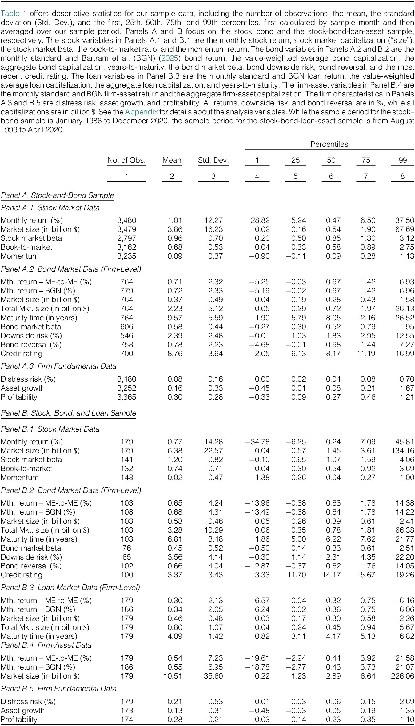
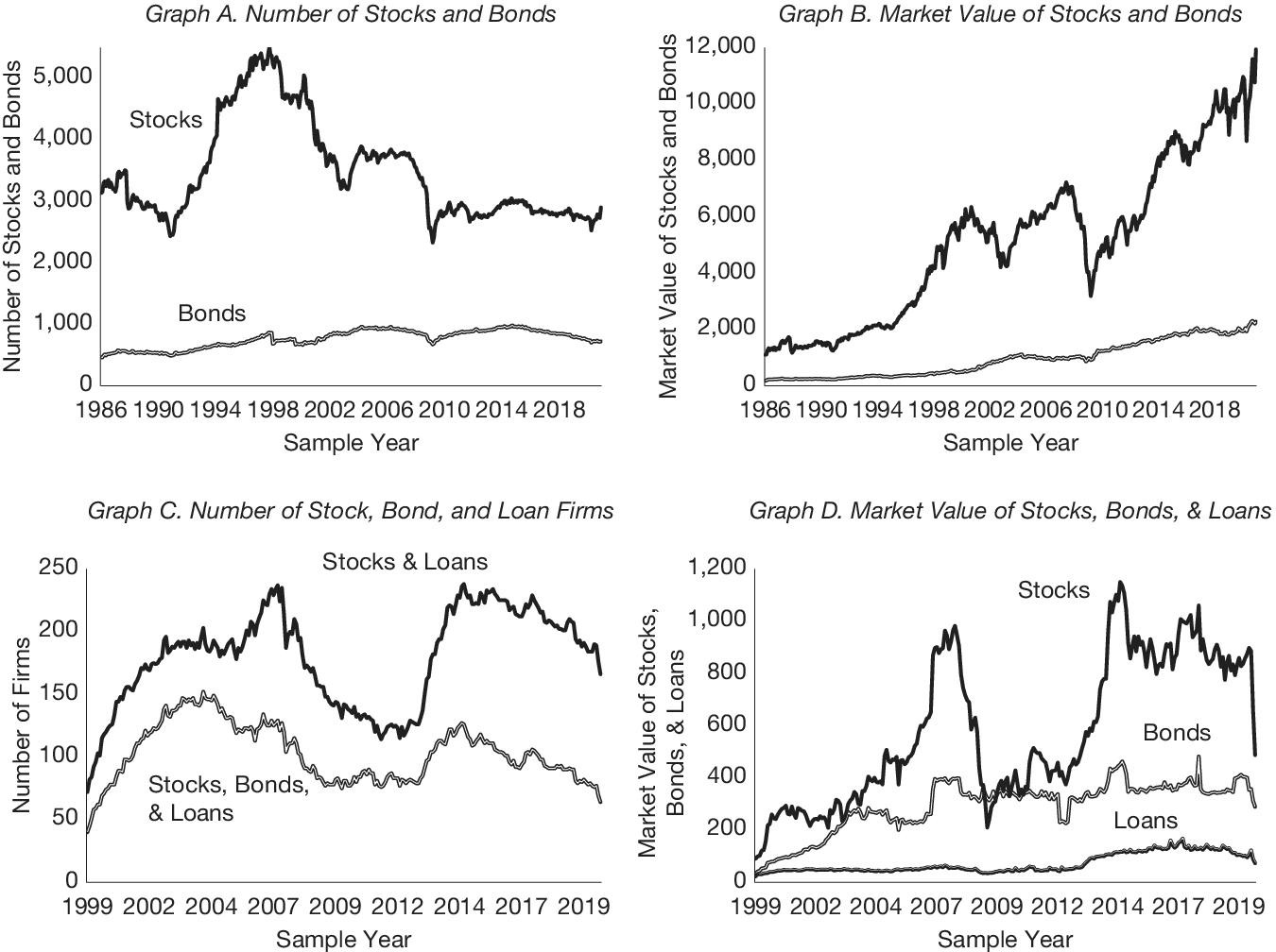
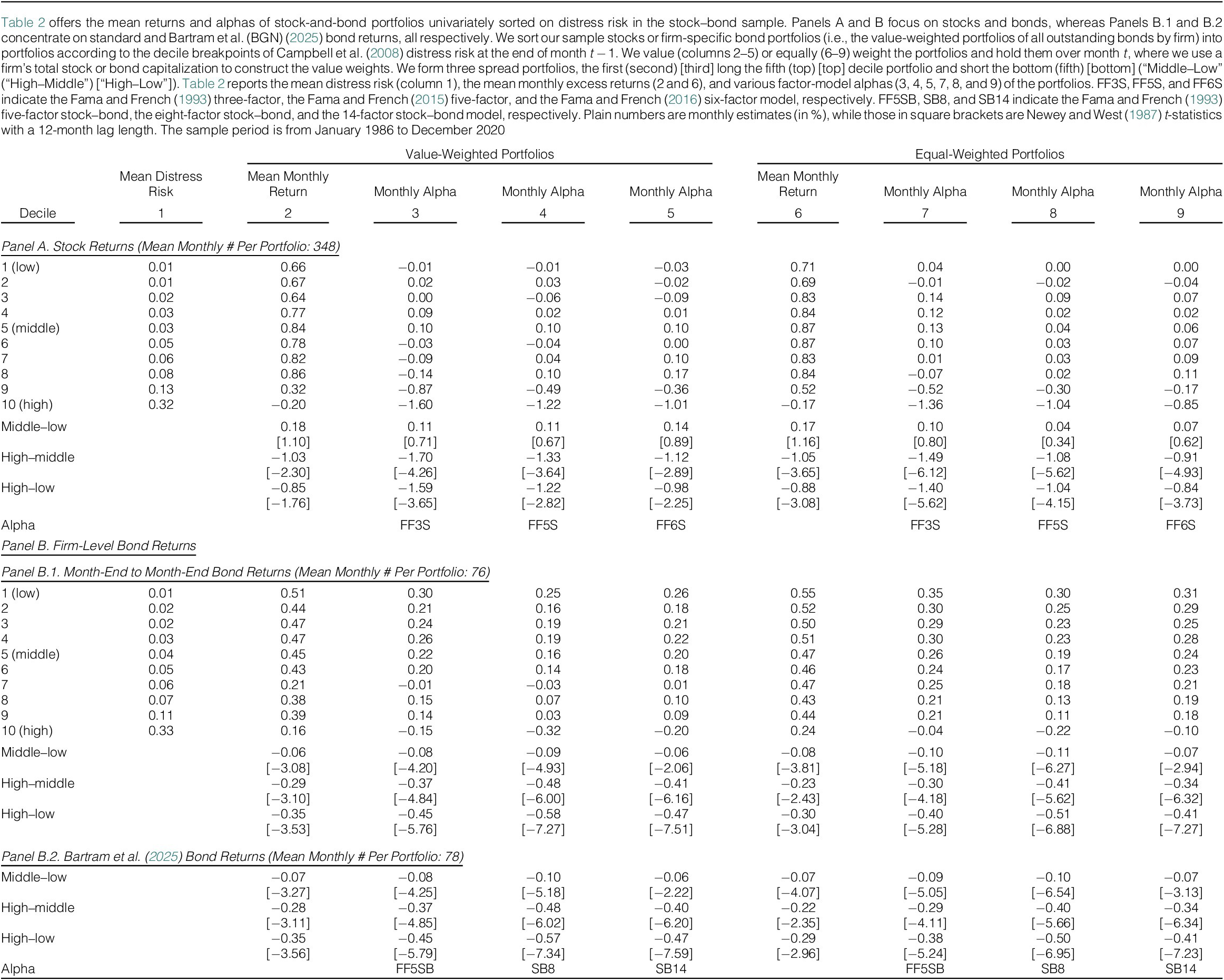
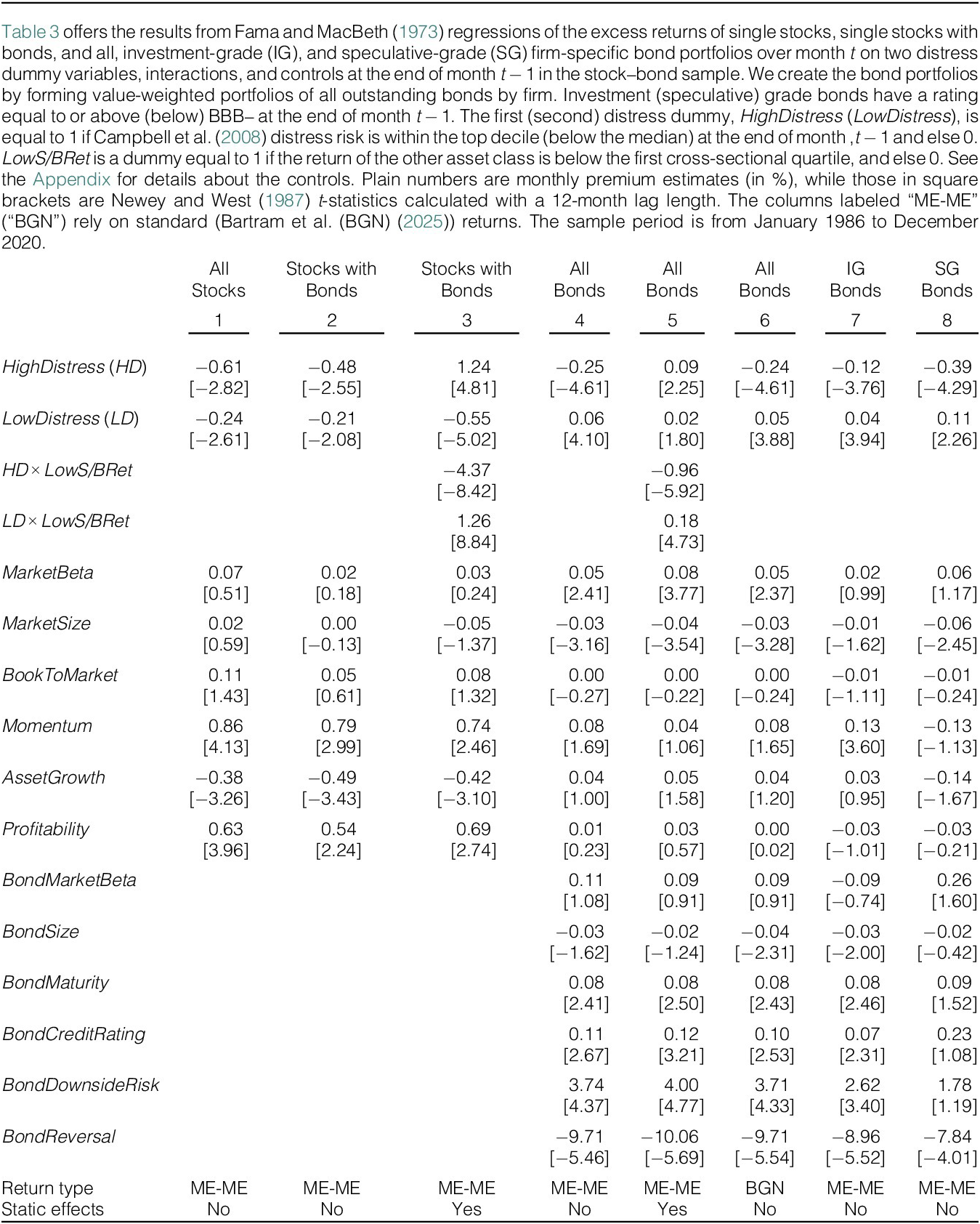
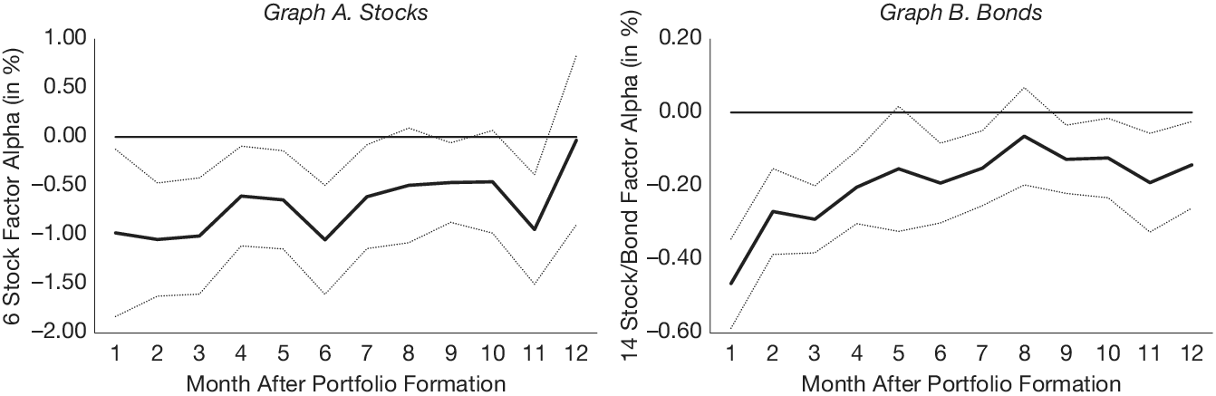


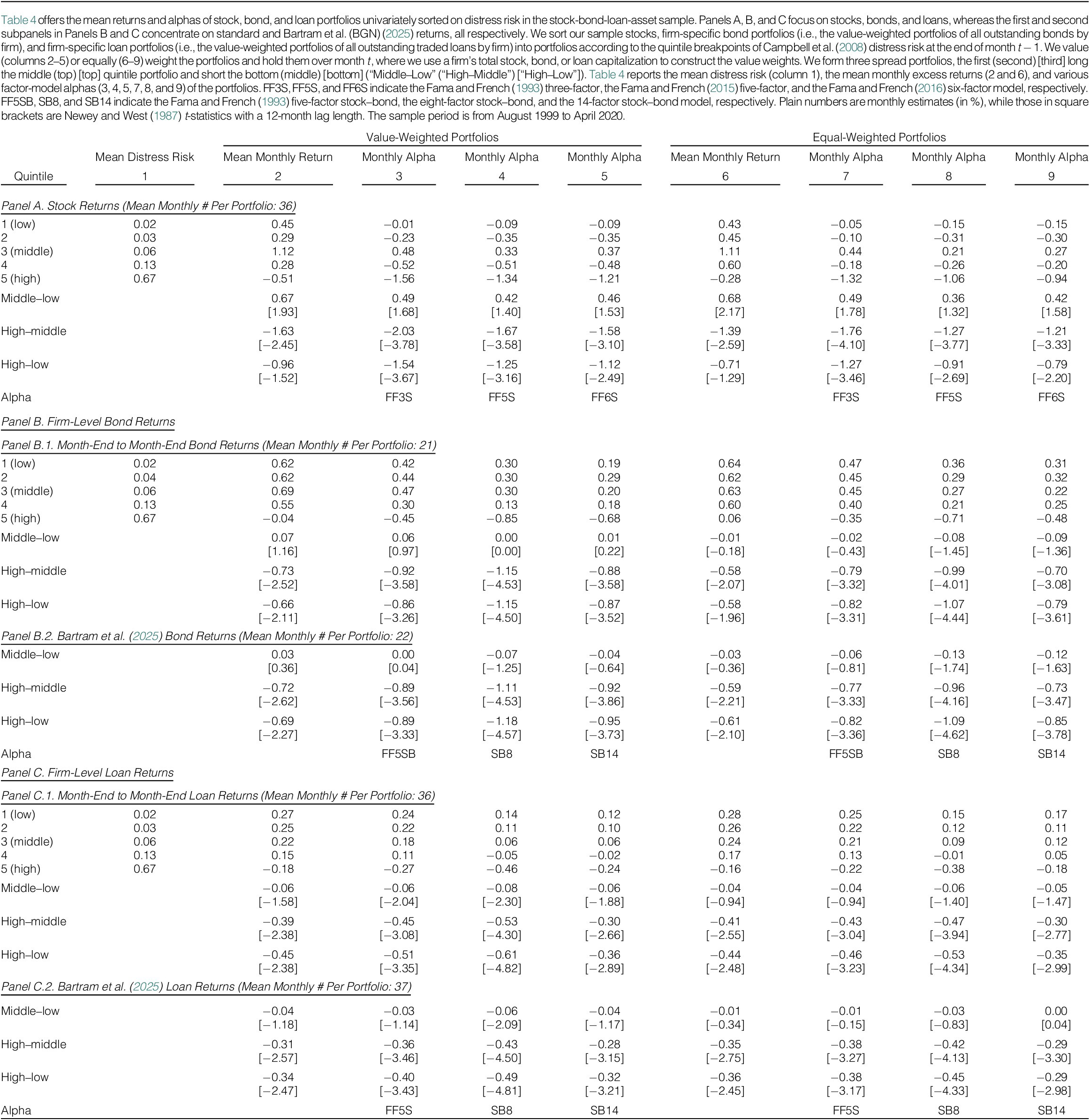
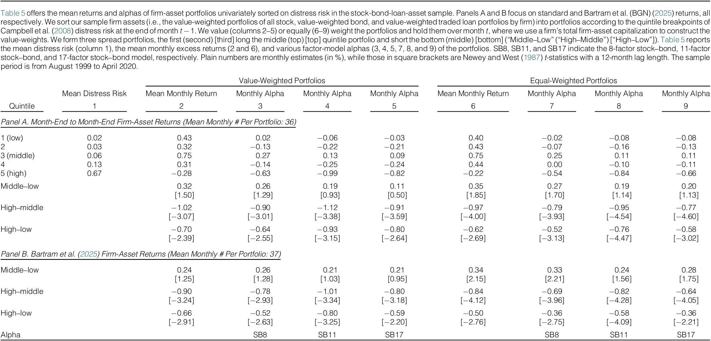
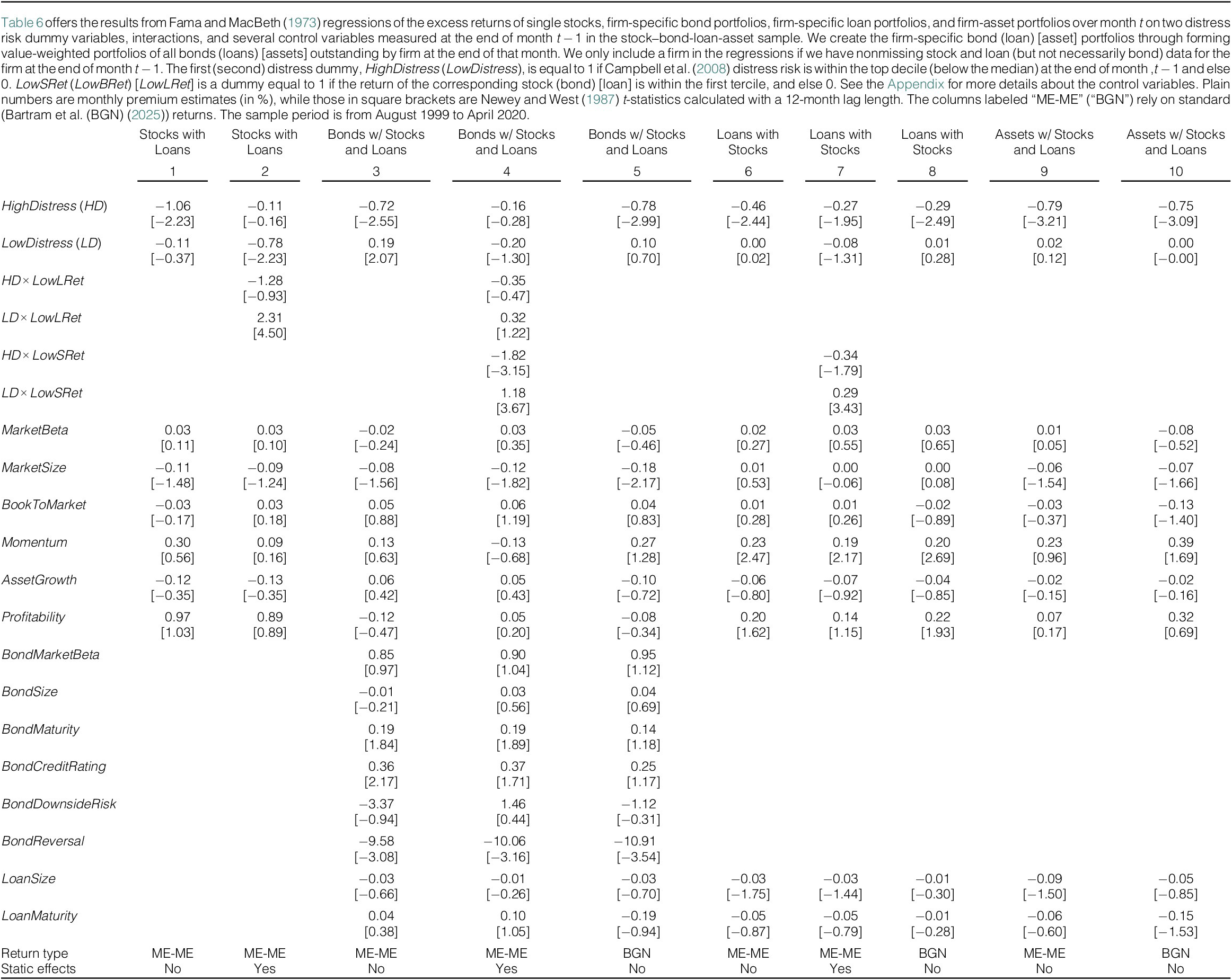
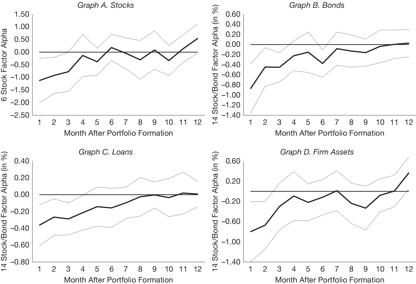


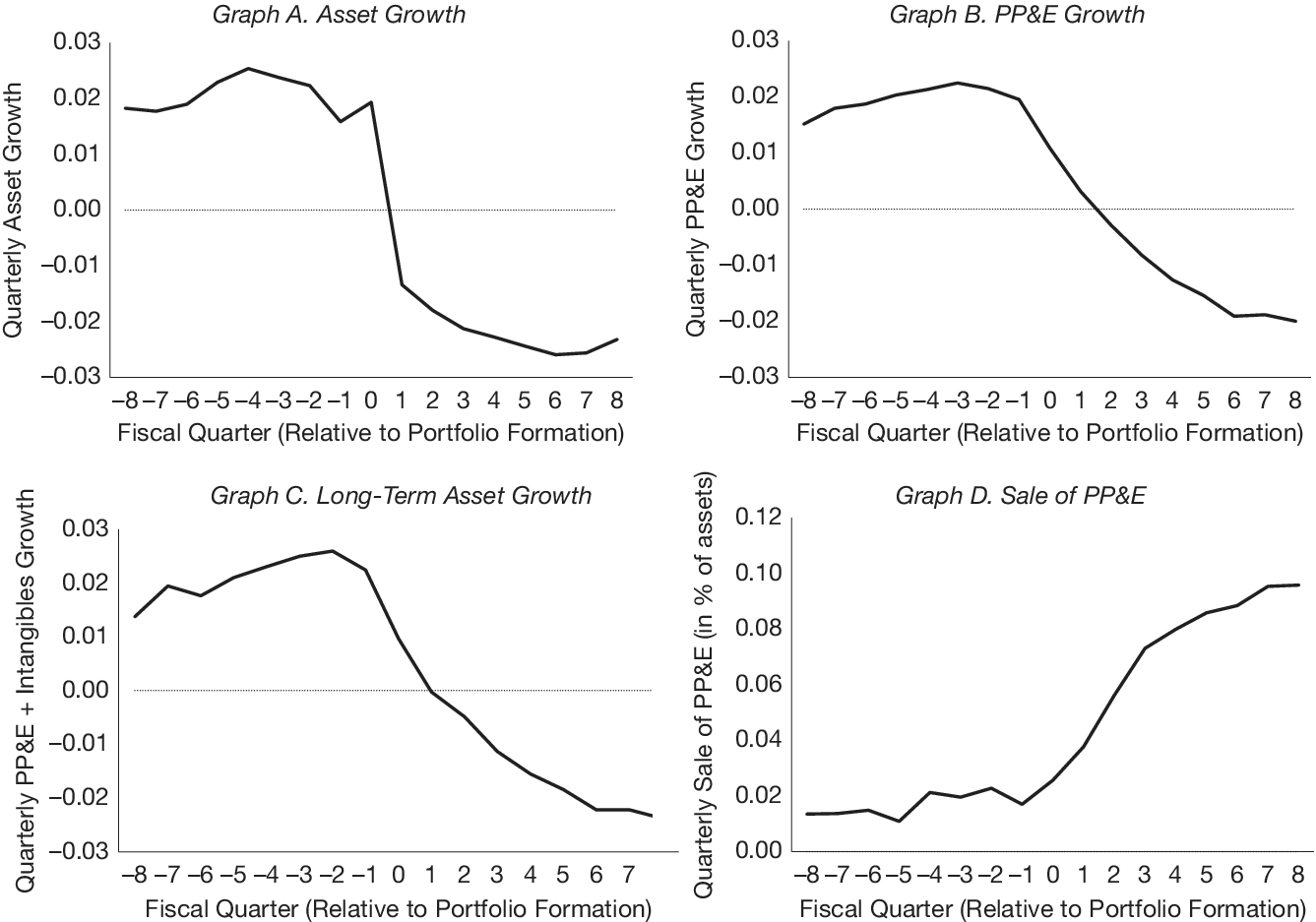
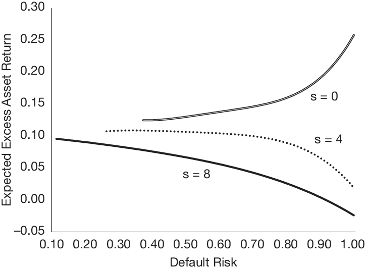

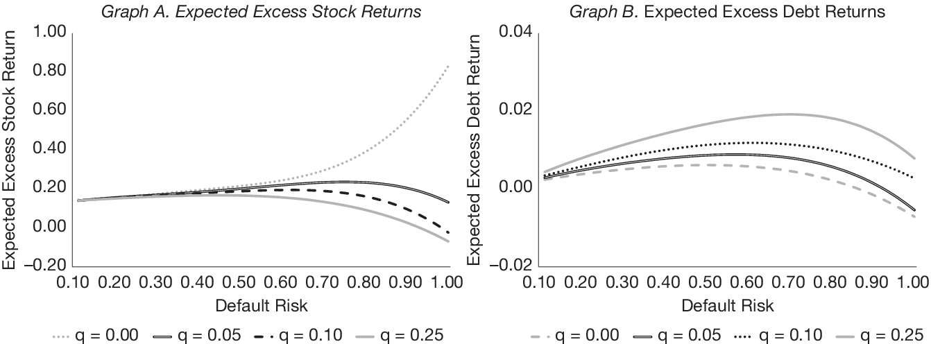


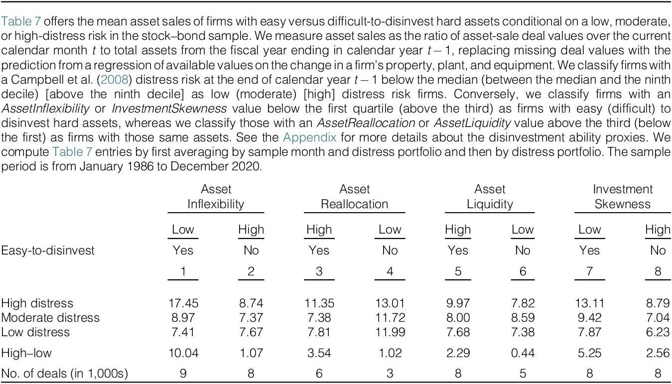
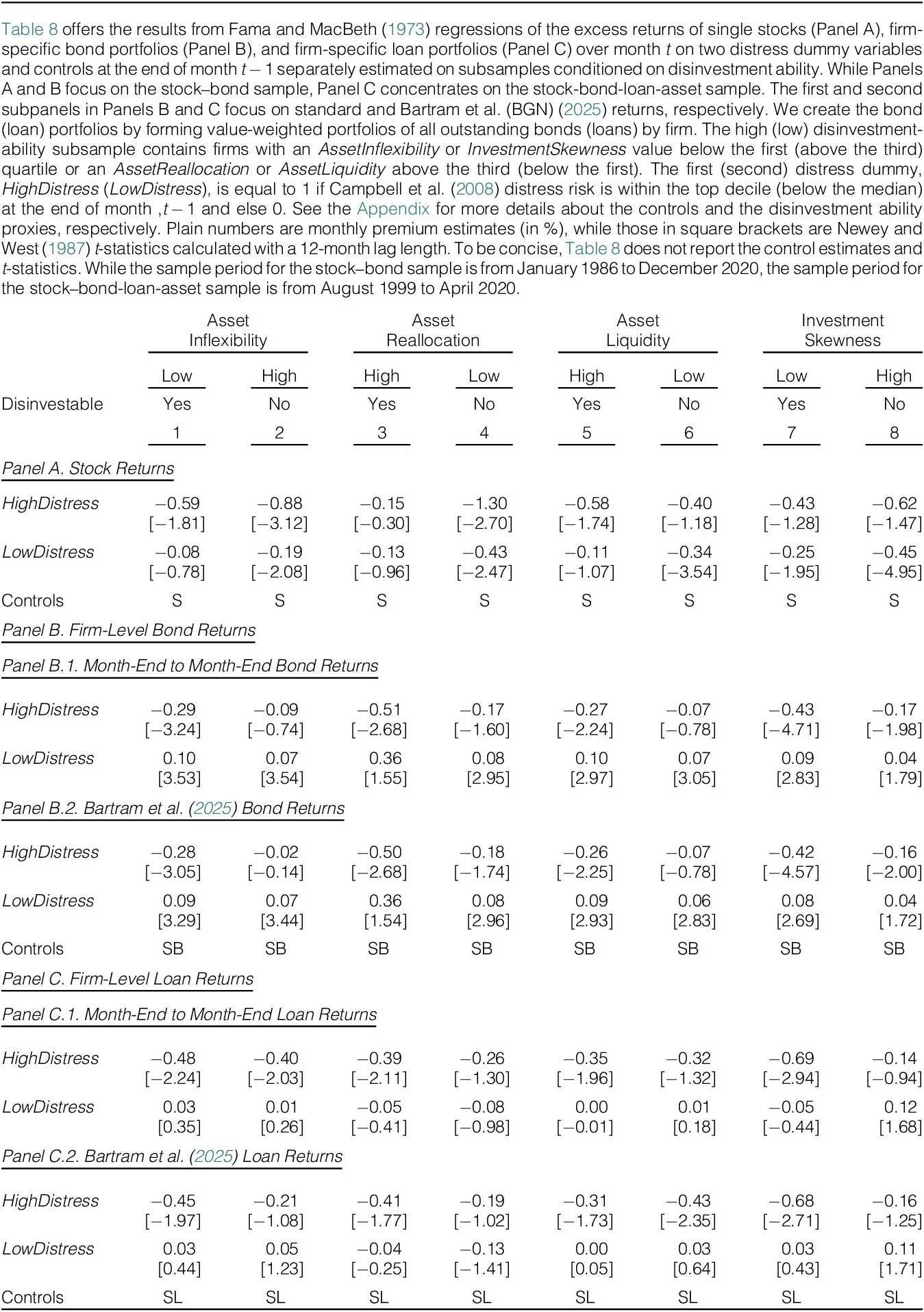
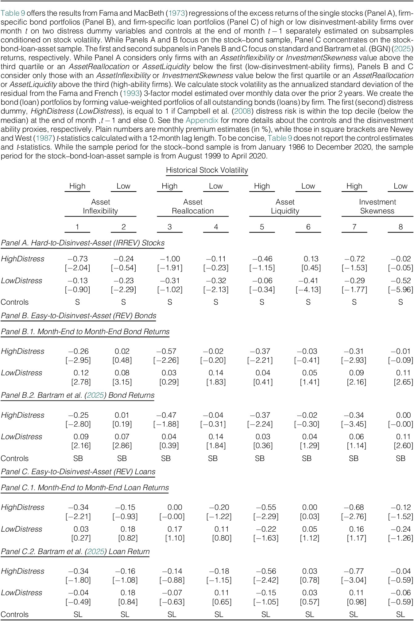


 Open access

