


1. Introduction
Snow covers drastically modify the energy and water fluxes at or near the land surface (Groisman, Karl & Knight Reference Groisman, Karl and Knight1994) even at long distances from the snow cover, and as a consequence, create significant feedback on the climate. They act as temporary water storage and control ground water recharge, making snow crucial to one-sixth of the world's population living in areas where solid precipitation dominates annual precipitation and runoff. The soil thermal properties and permafrost dynamics are dominated by the snow cover (Haberkorn et al. Reference Haberkorn, Wever, Hoelzle, Phillips, Kenner, Bavay and Lehning2017; Bender, Lehning & Fiddes Reference Bender, Lehning and Fiddes2020). Precise modelling of the snow cover properties, especially snow density and depth, is therefore vital in many applications, e.g. as input and validation data for climate models, hydrological models for irrigation and hydroelectricity, etc. Water vapour transport is a significant process in the snowpack in different respects such as snow metamorphism (Sturm & Benson Reference Sturm and Benson1997; Pfeffer & Mrugala Reference Pfeffer and Mrugala2002), snowpack stability and avalanches (Pfeffer & Mrugala Reference Pfeffer and Mrugala2002; Woo Reference Woo2012) and the thermal implications for climate applications (Slater et al. Reference Slater2001; Callaghan et al. Reference Callaghan2011). It has been demonstrated that current versions of one-dimensional snow models cannot simulate Arctic snowpacks because they omit an accurate description of water vapour transport (Domine et al. Reference Domine, Picard, Morin, Barrere, Madore and Langlois2019). For example, in the Arctic, observations by Trabant & Benson (Reference Trabant and Benson1972), Sturm & Benson (Reference Sturm and Benson1997) and Domine, Barrere & Sarrazin (Reference Domine, Barrere and Sarrazin2016) suggest that the density of layers close to the ground in thin snow covers can decrease by more than 100 kg m $^{-3}$ due to water vapour flux.
It has been previously discussed in the literature that depending on the snowpack, soil and meteorological conditions, water vapour transport may occur through both diffusion and convection (Trabant & Benson Reference Trabant and Benson1972; Johnson et al. Reference Johnson, Sturm, Perovich and Bens1987; Alley et al. Reference Alley, Saltzman, Cuffey and Fitzpatrick1990; Sturm & Johnson Reference Sturm and Johnson1991; Domine et al. Reference Domine, Barrere and Sarrazin2016, Reference Domine, Belke-Brea, Sarrazin, Arnaud, Barrere and Poirier2018). Jafari et al. (Reference Jafari, Gouttevin, Couttet, Wever, Michel, Sharma, Rossmann, Maass, Nicolaus and Lehning2020) discussed that diffusive water transport constitutes the lower limit for total water vapour transport and showed that diffusive vapour transport alone already reproduces lower densities at the base of the snowpack in some cases. However, in snowpacks under strong temperature gradients such as Arctic and sub-Arctic ones, in which weak snow layers composed of depth hoar crystals are rapidly formed (Sturm & Benson Reference Sturm and Benson1997; Taillandier et al. Reference Taillandier, Domine, Simpson, Sturm, Douglas and Severin2006; Derksen et al. Reference Derksen, Silis, Sturm, Holmgren, Liston, Huntington and Solie2009; Domine et al. Reference Domine, Barrere, Sarrazin, Morin and Arnaud2015), water vapour transport is hypothesized to mainly be driven by natural convection. It has been concluded that significant convection must occur in snowpacks to explain the observations, namely: (1) the measured rates of densification and density changes for snow in Fairbanks by Trabant & Benson (Reference Trabant and Benson1972), (2) significant horizontal thermal gradients and incoherent temporal variations of horizontal temperature patterns at their study site by Sturm & Johnson (Reference Sturm and Johnson1991) and (3) the near-total disappearance of basal depth hoar at Bylot Island by Domine et al. (Reference Domine, Barrere and Sarrazin2016).
Snow–atmosphere coupling with high uncertainty in the magnitude of perturbation within the snow is another mechanism which may influence the heat and mass regime of the snowpack surface and if strong enough in deeper snow layers. Colbeck (Reference Colbeck1989) introduced three different such wind pumping or ventilation mechanisms, namely barometric pressure variations, wind turbulence and steady wind flow over topography, and concluded the last one could be strong enough to induce significant air moving through snow. Waddington, Cunningham & Harder (Reference Waddington, Cunningham and Harder1996) concluded that the dry deposition flux due to turbulent ventilation should be very small and that the air velocity through the snow surface by wind turbulence is of the order of 0.01 cm s $^{-1}$. Sokratov & Sato (Reference Sokratov and Sato2000) estimated the wind-induced horizontal air flux to be of the order of
  $10^{-2}$ m s
 $^{-1}$ while Albert & McGilvary (Reference Albert and McGilvary1992) and Albert (Reference Albert1993) reported much larger values for air flux by wind pumping ranging from
  $10^{-7}$ to 0.1 m s
 $^{-1}$. Bartlett & Lehning (Reference Bartlett and Lehning2011) in agreement with Colbeck (Reference Colbeck1989) and Waddington et al. (Reference Waddington, Cunningham and Harder1996) concluded that ventilation should have a minimal impact on heat transfer under typical conditions. These studies suggest that measurable effects only occur to a small penetration depth (Colbeck Reference Colbeck1989; Waddington et al. Reference Waddington, Cunningham and Harder1996; Bartlett & Lehning Reference Bartlett and Lehning2011).
Observations cannot distinguish between different types of vapour transport and represent a mixture of effects such as snow settling, vapour transport and wind compaction (Sommer, Lehning & Fierz Reference Sommer, Lehning and Fierz2018). Therefore, a sound modelling of water vapour transport needs to take into account natural convection as a possible mechanism of density change and observations need to be explained by modelling. As reviewed by Jafari et al. (Reference Jafari, Gouttevin, Couttet, Wever, Michel, Sharma, Rossmann, Maass, Nicolaus and Lehning2020), previous attempts to numerically study water vapour transport in snow and its effects on snow properties consider diffusion only. It is furthermore not possible to explicitly model convection with phase change in a one-dimensional snow model. Thus, in this work, the convective water vapour transport is numerically investigated in snowpacks, using a volume-averaged two-phase model in which each phase is treated separately and interactions between the phases are modelled. The numerical implementation is in a two-dimensional domain. Performance of the present model for natural convection without mass transfer was validated by comparison with available numerical benchmarks. When including phase change and the associated local density changes, a considerable impact of natural convection on the snow density distribution with a layer of significantly lower density at the bottom of the snowpack and a layer of higher density located at the top is observed. This is consistent with measurements of Domine et al. (Reference Domine, Barrere and Sarrazin2016), who find that the density increase for the wind slabs overlying depth hoar may be attributed to upward water vapour transfer and its deposition.
2. Mathematical models
Whilst acknowledging but neglecting the effects of ventilation and snow compaction, to start with a tractable model and focus on the effect of convection, water vapour transport due to natural convection in idealized snowpacks is investigated numerically using an Eulerian–Eulerian two-phase approach. To do so, the volume-averaging method is applied to the conservation of mass, momentum and energy which are valid within each phase up to the interface between phases. In this paper, the snowpack is considered as a two-phase (humid air, ice) porous medium for which the phase change between the water vapour component in the gas mixture and ice is simulated. The detailed explanation, derivations and operations constituting the volume-averaging method can be found in (Whitaker Reference Whitaker1999; Faghri & Zhang Reference Faghri and Zhang2006). Note that, in this paper, all the phase properties presented as  $\left \langle - \right \rangle ^{g}$ and
  $\left \langle - \right \rangle ^{i}$ are the intrinsic phase averages for the gas and ice phases, respectively, while the extrinsic averages are shown as the operator
  $\left \langle - \right \rangle$.
2.1. Mass conservation
The volume-averaged mass conservation equations for the gas mixture (humid air), water vapour component and ice phase are given respectively as
 \begin{gather} \frac{\partial}{\partial t} \left(\epsilon_{g} \left\langle \rho_{g} \right\rangle^{g}\right)+ \boldsymbol{\nabla}\boldsymbol{\cdot} \left( \left\langle \rho_{g} \right\rangle^{g} \left\langle \boldsymbol{U}_{g} \right\rangle\right) = \dot{m_{iv}}, \end{gather}
 \begin{gather} \frac{\partial}{\partial t}\left(\epsilon_{g} \left\langle \rho_{v} \right\rangle^{g}\right)+ \boldsymbol{\nabla}\boldsymbol{\cdot} \left( \left\langle \rho_{v} \right\rangle^{g} \left\langle \boldsymbol{U}_{g} \right\rangle\right) = \boldsymbol{\nabla}\boldsymbol{\cdot} (D_{{eff},s} \boldsymbol{\nabla} \left\langle \rho_{v} \right\rangle^{g})+ \dot{m_{iv}}, \end{gather}
 \begin{gather} \rho_{i} \frac{\partial \epsilon_{i}}{\partial t} ={-}\dot{m_{iv}}, \end{gather}
where  $\epsilon _{g}$ and
  $\epsilon _{i}$ are the volume fractions for the gas and ice phases respectively,
  $\left \langle \boldsymbol {U}_{g} \right \rangle$ is the bulk gas-phase velocity vector (also known as superficial, extrinsic, filtration, Darcy or seepage velocity),
  $\left \langle \rho _{g} \right \rangle ^{g}$ is the gas mixture density,
  $\left \langle \rho _{v} \right \rangle ^{g}$ is the water vapour density,
  $\rho _{i}$ is the ice density,
  $\dot {m_{iv}}$ represents mass source (or sink) per unit volume due to the phase change (subscript
  ${iv}$ refers to the mass transfer from ice to vapour while
  ${vi}$ from vapour to ice) and
  $D_{{eff},s}$ is the effective water vapour diffusivity in snow. A brief review of effective diffusivity and its enhancement in snow has been made in Jafari et al. (Reference Jafari, Gouttevin, Couttet, Wever, Michel, Sharma, Rossmann, Maass, Nicolaus and Lehning2020). Based on an analytical model developed first by Foslien (Reference Foslien1994) and then extended by Hansen & Foslien (Reference Hansen and Foslien2015), the following parameterization for
  $D_{{eff},s}$ is used:
 \begin{equation} D_{{eff},s}=\epsilon_{i} \epsilon_{g} D_{v,a}+\epsilon_{g} \frac{k_i D_{v,a}}{\epsilon_{i}\left(k_a+L_{iv} D_{v,a} \dfrac{{\rm d}\rho_{vs}}{{\rm d}T}\right)+\epsilon_{g} k_i}, \end{equation}
where  $k_i$ and
  $k_a$ are the thermal conductivities for the air and ice components of snow respectively,
  $D_{v,a}$ is the water vapour diffusion coefficient in air,
  $\rho _{vs}$ is the saturation water vapour density calculated at the interface temperature between two phases and
  $L_{iv}$ is the latent heat of sublimation. Following Albert & McGilvary (Reference Albert and McGilvary1992),
  $\dot {m_{iv}}$ may be evaluated as
 \begin{equation} \dot{m_{iv}}=h_m a_s (\rho_{vs}-\left\langle \rho_{v} \right\rangle^{g}). \end{equation}
 In (2.5),  $h_m$ is the mass transfer coefficient and
  $a_s=6 \epsilon _{i}/d_{p}$ is the specific surface area of snow with optical grain diameter of
  $d_{p}$ (Calonne et al. Reference Calonne, Geindreau, Flin, Morin, Lesaffre, Rolland du Roscoat and Charrier2012). Jafari et al. (Reference Jafari, Gouttevin, Couttet, Wever, Michel, Sharma, Rossmann, Maass, Nicolaus and Lehning2020) discussed that the entire specific surface area may be not active for mass transfer, and hence justified the choice of the formulation as
  $h_m= \rho _i/(\mathcal {B} \rho _{v,s})$ proposed respectively by Calonne, Geindreau & Flin (Reference Calonne, Geindreau and Flin2014) and Ebner et al. (Reference Ebner, Andreoli, Schneebeli and Steinfeld2015). Here, the interface kinetic growth coefficient was found to be
  $\mathcal {B}=9.7 \times 10^9$ s m
 $^{-1}$ from the experiments of sublimation and deposition on the ice structure with and without advective flows in snow. The degree of over- or under-saturation,
  $\sigma =\left (\left \langle \rho _{v} \right \rangle ^{g}-\rho _{v,s}\right )/\rho _{v,s}$, is directly related to the phase change rate
  $\dot {m_{iv}}$ (the divergence of the vapour flux) (Jafari et al. Reference Jafari, Gouttevin, Couttet, Wever, Michel, Sharma, Rossmann, Maass, Nicolaus and Lehning2020) and can be used as a diagnostic variable to quantify the intensity of the phase change rate. Hence, the phase change rate
  $\dot {m_{iv}}$ can be written as
 \begin{equation} \dot{m_{iv}}={-} \frac{6 \epsilon_{i} \rho_i}{\mathcal{B} d_{p}} \sigma. \end{equation}
2.2. Momentum
With the pore Reynolds number  $Re_{p}=\rho _{g} | \left \langle \boldsymbol {U}_{g} \right \rangle | d_p/\mu$ (based on particle size,
  $d_{p}$) less than 10, the advective and inertial terms are negligible (Gray & O'Neill Reference Gray and O'Neill1976; Ganesan & Poirier Reference Ganesan and Poirier1990; Faghri & Zhang Reference Faghri and Zhang2006; Nield & Bejan Reference Nield and Bejan2017) and thus the volume-averaged momentum equation for gas flow through the snowpack as a porous medium with variable porosity can be simplified to the Darcy–Forchheimer equation (Ward Reference Ward1964; Faghri & Zhang Reference Faghri and Zhang2006; Nield & Bejan Reference Nield and Bejan2017) as
 \begin{equation} {-}\frac{\mu}{K} \left\langle \boldsymbol{U}_{g} \right\rangle -\frac{ \left\langle \rho_{g} \right\rangle^{g} c_{F} }{\sqrt{K}} \left| \left\langle \boldsymbol{U}_{g} \right\rangle \right| \left\langle \boldsymbol{U}_{g} \right\rangle -\boldsymbol{\nabla}\left\langle P_{g} \right\rangle^{g} +\left\langle \rho_{g} \right\rangle^{g}\boldsymbol{g} = 0, \end{equation}
where  $\mu$ is the dynamic viscosity of the air,
  $K$ is the intrinsic permeability of the porous medium,
  $c_{F}$ is a dimensionless form-drag constant and
  $\left \langle P_{g} \right \rangle ^{g}$ is the gas mixture pressure. In (2.7), the first and second terms refer to the Darcian relationship due to the viscous surface friction and the quadratic drag (or the nonlinear form drag) due to solid obstacles, respectively (Faghri & Zhang Reference Faghri and Zhang2006; Nield & Bejan Reference Nield and Bejan2017). The quadratic drag is significant when
  $1< Re_{p}<10$, otherwise it is negligible compared with the Darcian term (Faghri & Zhang Reference Faghri and Zhang2006; Nield & Bejan Reference Nield and Bejan2017). To extract the driving force associated with the gas density gradient in the momentum equation (2.7), the hydrostatic pressure contribution is separated from total gas pressure as
  $\left \langle P_{g} \right \rangle ^{g}=\left \langle P_{g_d} \right \rangle ^{g}-\left \langle \rho _{g} \right \rangle ^{g} g z$. Hence, the momentum equation may be read equivalently as
 \begin{equation} {-}\frac{\mu}{K} \left\langle \boldsymbol{U}_{g} \right\rangle -\frac{ \left\langle \rho_{g} \right\rangle^{g} c_{F} }{\sqrt{K}} \left| \left\langle \boldsymbol{U}_{g} \right\rangle \right| \left\langle \boldsymbol{U}_{g} \right\rangle -\boldsymbol{\nabla}\left\langle P_{g_d} \right\rangle^{g} +\boldsymbol{\nabla}\left\langle \rho_{g} \right\rangle^{g} \left|g z \right| = 0. \end{equation}
Using three-dimensional images of snow microstructure, Calonne et al. (Reference Calonne, Geindreau, Flin, Morin, Lesaffre, Rolland du Roscoat and Charrier2012) proposed the following regression for the snow permeability:
 \begin{equation} K = \frac{3}{4} d_{p}^{2}~\exp({-}0.013 \rho_{i} \epsilon_{i}). \end{equation}
 Assuming Ergun's equation for momentum, the dimensionless form-drag constant can be evaluated by  $c_{F}=\alpha \gamma ^{-1/2} \epsilon _{g}^{-3/2}$ as an ad hoc procedure with
  $\alpha =1.75$ and
  $\gamma =150$ (Nield & Bejan Reference Nield and Bejan2017).
2.3. Energy
Neglecting the effect of viscous dissipation on natural convection in a porous medium (Nield & Bejan Reference Nield and Bejan2017), the intrinsic volume-averaged energy equations in terms of enthalpy  $\left \langle h_{g} \right \rangle ^{g}$ for the gas phase and
  $\left \langle h_{i} \right \rangle ^{i}$ for the ice phase with local thermal non-equilibrium are derived respectively as (Faghri & Zhang Reference Faghri and Zhang2006; Nield & Bejan Reference Nield and Bejan2017)
 $$\begin{gather} \frac{\partial}{\partial t}\left(\epsilon_{g} \left\langle \rho_{g} \right\rangle^{g} \left\langle h_{g} \right\rangle^{g}\right) + \boldsymbol{\nabla}\boldsymbol{\cdot} \left( \left\langle \rho_{g} \right\rangle^{g} \left\langle h_{g} \right\rangle^{g} \left\langle \boldsymbol{U}_{g} \right\rangle\right) ={-} \boldsymbol{\nabla}\boldsymbol{\cdot} \left\langle \boldsymbol{q}_{g}^{\prime\prime}\mkern-1.2mu \right\rangle^{g}\nonumber\\ - \boldsymbol{\nabla}\boldsymbol{\cdot} \left[ \left\langle h_{v} \right\rangle^{g} \left\langle J_{v} \right\rangle + \left\langle h_{a} \right\rangle^{g} \left\langle J_{a} \right\rangle \right] +\epsilon_{g} \frac{\partial}{\partial t} \left\langle P_{g} \right\rangle^{g} +\left\langle \boldsymbol{U}_{g} \right\rangle \boldsymbol{\cdot} \boldsymbol{\nabla}\left\langle P_{g} \right\rangle^{g}\nonumber\\ +\dot{m_{iv}} \left\langle h_{v,I} \right\rangle^{g} +\left\langle q_{I,g} \right\rangle, \end{gather}$$
 \begin{gather} \rho_{i} \frac{\partial}{\partial t}\left(\epsilon_{i} \left\langle h_{i} \right\rangle^{i}\right) ={-} \boldsymbol{\nabla}\boldsymbol{\cdot} \left\langle \boldsymbol{q}_{i}^{\prime\prime}\mkern-1.2mu \right\rangle^{i} +\dot{m_{vi}} \left\langle h_{i,I} \right\rangle^{i} +\left\langle q_{I,i} \right\rangle. \end{gather}
 The subscripts  $a$ and
  $v$ correspond to the dry air and water vapour components respectively. The first two terms on the right-hand side of (2.10a) represent the divergence of the conductive heat flux and the interdiffusional convection (the transfer of enthalpy with vapour and air diffusive fluxes as
  $\left \langle J_{v} \right \rangle$ and
  $\left \langle J_{a} \right \rangle$), respectively. The fourth term on the right-hand side of (2.10a) is the reversible rate of energy change per unit volume associated with compression. In (2.10),
  $\left \langle \boldsymbol {q}_{g}^{\prime \prime }\mkern -1.2mu \right \rangle ^{g}$ and
  $\left \langle \boldsymbol {q}_{i}^{\prime \prime }\mkern -1.2mu \right \rangle ^{i}$ are the conductive heat fluxes in the gas and ice phases respectively,
  $\left \langle q_{I,g} \right \rangle$ and
  $\left \langle q_{I,i} \right \rangle$ are the conductive heat transfer per unit volume from the interface to the related phases and the terms
  $\dot {m_{iv}} \left \langle h_{v,I} \right \rangle ^{g}$ and
  $\dot {m_{vi}} \left \langle h_{i,I} \right \rangle ^{g}$ are the interphase enthalpy exchange due to phase change, in which
  $\left \langle h_{v,I} \right \rangle ^{g}$ and
  $\left \langle h_{i,I} \right \rangle ^{i}$ are the intrinsic volume-averaged enthalpies of the water vapour and ice, respectively, calculated at the interface temperature
  $T_{I}$. Assuming humid air as being an ideal gas mixture and using the ideal gas equation of state for the water vapour and dry air components, the enthalpy
  $\left \langle h_{g} \right \rangle ^{g}$, the specific heat capacity
  $\left \langle c_{pg} \right \rangle ^{g}$, the molecular mass
  $\left \langle M_{g} \right \rangle ^{g}$ and the density of the gas mixture are evaluated as
 \begin{gather} \left\langle h_{g} \right\rangle^{g}=\frac{ \left\langle \rho_{v} \right\rangle^{g} \left\langle h_{v} \right\rangle^{g} + \left\langle \rho_{a} \right\rangle^{g} \left\langle h_{a} \right\rangle^{g} }{ \left\langle \rho_{g} \right\rangle^{g} }, \end{gather}
 \begin{gather} \left\langle c_{pg} \right\rangle^{g}=\frac{ \left\langle \rho_{v} \right\rangle^{g} c_{pv} + \left\langle \rho_{a} \right\rangle^{g} c_{pa} }{ \left\langle \rho_{g} \right\rangle^{g} }, \end{gather}
 \begin{gather} \left\langle \rho_{g} \right\rangle^{g}= \left\langle \rho_{v} \right\rangle^{g} + \left\langle \rho_{a} \right\rangle^{g} = \frac{ \left\langle P_{g} \right\rangle^{g} \left\langle M_{g} \right\rangle^{g} }{ R_{u} \left\langle T_{g} \right\rangle^{g} }, \end{gather}
 \begin{gather} \left\langle \rho_{a} \right\rangle^{g}= \frac{ \left\langle P_{a} \right\rangle^{g} M_{a} }{ R_{u} \left\langle T_{g} \right\rangle^{g} }, \end{gather}
 \begin{gather} \left\langle \rho_{v} \right\rangle^{g}= \frac{ \left\langle P_{v} \right\rangle^{g} M_{v} }{ R_{u} \left\langle T_{g} \right\rangle^{g} }, \end{gather}
 \begin{gather} \left\langle M_{g} \right\rangle^{g}= \frac{ \left\langle \rho_{g} \right\rangle^{g} }{ \left\langle \rho_{a} \right\rangle^{g}/M_{a} + \left\langle \rho_{v} \right\rangle^{g}/M_{v} }. \end{gather}
In (2.11),  $R_{u}$ is the universal gas constant,
  $M_{v}$ and
  $M_{a}$ are the molecular mass,
  $c_{pv}$ and
  $c_{pa}$ are the specific heat capacity and finally
  $\left \langle P_{v} \right \rangle ^{g}$ and
  $\left \langle P_{a} \right \rangle ^{g}$ are the partial pressure for the water vapour and dry air components respectively. The zero point of the enthalpy for dry air and liquid water is chosen at the reference temperature
  $T_{ref}=273.15$ K. Therefore, the enthalpies of dry air, water vapour and ice are given as (Russo et al. Reference Russo, Kuerten, Van Der Geld and Geurts2014)
 \begin{gather} \left\langle h_{v} \right\rangle^{g} = \left\langle h_{v} \right\rangle^{g}(T=T_{ref})+c_{pv}\left(\left\langle T_{g} \right\rangle^{g}-T_{ref}\right) = L_{wv}+c_{pv}\left(\left\langle T_{g} \right\rangle^{g}-T_{ref}\right), \end{gather}
 \begin{gather} \left\langle h_{i} \right\rangle^{i} = \left\langle h_{i} \right\rangle^{i}(T=T_{ref})+c_{pi} \left(\left\langle T_{i} \right\rangle^{i}-T_{ref}\right) ={-}L_{iw}+c_{pi} \left(\left\langle T_{i} \right\rangle^{i}-T_{ref}\right), \end{gather}
 \begin{gather} \left\langle h_{a} \right\rangle^{g} = c_{pa} \left(\left\langle T_{g} \right\rangle^{g}-T_{ref}\right), \end{gather}
where  $L_{iw}$ and
  $L_{wv}$ are the latent heat of fusion and evaporation respectively. Given that the interfacial energy terms associated with surface tension, work done by pressure and interfacial shear stress work (the conversion of mechanical to thermal energy) are usually negligible with respect to the large energy exchange due to phase change, the energy balance at the interface can be written as (Faghri & Zhang Reference Faghri and Zhang2006; Ishii & Hibiki Reference Ishii and Hibiki2010; Hugelius et al. Reference Hugelius2014)
 \begin{equation} \dot{m_{iv}} \left\langle h_{v,I} \right\rangle^{g} +\left\langle q_{I,g} \right\rangle +\dot{m_{vi}} \left\langle h_{i,I} \right\rangle^{i} +\left\langle q_{I,i} \right\rangle = 0. \end{equation}
To obtain the heat transfer from the interface to the gas phase  $\left \langle q_{I,g} \right \rangle$, Newton's law of cooling is used as follows:
 \begin{equation} \left\langle q_{I,g} \right\rangle = h_{c} a_{s} (T_{I} - \left\langle T_{g} \right\rangle^{g}), \end{equation}
where  $h_{c}$ is the heat transfer coefficient and
  $a_{s}$ is the specific surface area of the porous medium. Substituting (2.14) into (2.13) with
  $\dot {m_{vi}}=-\dot {m_{iv}}$, the heat transfer from the interface to the ice phase
  $\left \langle q_{I,i} \right \rangle$ may be calculated as
 \begin{equation} \left\langle q_{I,i} \right\rangle ={-}h_{c} a_{s} \left(\left\langle T_{g} \right\rangle^{g} -T_{I}\right) +\dot{m_{iv}} \left(\left\langle h_{i,I} \right\rangle^{i} - \left\langle h_{v,I} \right\rangle^{g}\right). \end{equation}
 Based on the temporal term in the bulk heat transfer equation including both phases (homogeneous mixture model), the interface temperature  $T_{I}$ may be evaluated as
 \begin{gather} T_{I}= w_{g} \left\langle T_{g} \right\rangle^{g} + w_{i} \left\langle T_{i} \right\rangle^{i}, \end{gather}
 \begin{gather} w_{g}=\frac{ \epsilon_{g} \left\langle \rho_{g} \right\rangle^{g} c_{pg} }{ \epsilon_{g} \left\langle \rho_{g} \right\rangle^{g} c_{pg} + \epsilon_{i} \rho_{i} c_{pi} }, \end{gather}
 \begin{gather} w_{i}=\frac{ \epsilon_{i} \rho_{i} c_{pi} }{ \epsilon_{g} \left\langle \rho_{g} \right\rangle^{g} c_{pg} + \epsilon_{i} \rho_{i} c_{pi} }. \end{gather}
 Based on analogies between heat and mass transfer (Bird, Stewart & Lightfoot Reference Bird, Stewart and Lightfoot1961; Faghri & Zhang Reference Faghri and Zhang2006; Bergman et al. Reference Bergman, Incropera, DeWitt and Lavine2011), it follows that the dimensionless temperature gradient expressed by the Nusselt number  $Nu=h_{c}d_{p}/k_{a}=f(Re_p,Pr)$ and concentration gradient expressed by Sherwood number
  $Sh=h_{m}d_{p}/D_{v,a}=f(Re_p,Sc)$ are similar and we assume
  $Nu=Sh$. Here
  $Sc$ is the Schmidt number, the ratio of kinematic viscosity and mass diffusivity, and
  $Pr$ is the heat transfer equivalent of the Schmidt number. For gases,
  $Sc$ and
  $Pr$ have similar values (
 ${\approx }0.7$) and this is used as the basis for simple heat and mass transfer analogies. Therefore, the heat transfer coefficient
  $h_{c}$ may be related to the mass transfer coefficient
  $h_{m}$ as
 \begin{equation} h_{c}=\frac{h_{m} k_{a}}{D_{v,a}}. \end{equation}
Combining (2.11), (2.12), (2.14), (2.15) and (2.16) with (2.10), the energy equations in term of temperature for the gas and ice phases are derived as
 \begin{align} &\frac{\partial}{\partial t}\left(\epsilon_{g} \left\langle \rho_{g} \right\rangle^{g} c_{pg} \left\langle T_{g} \right\rangle^{g}\right) + \boldsymbol{\nabla}\boldsymbol{\cdot} \left( \left\langle \rho_{g} \right\rangle^{g} c_{pg} \left\langle T_{g} \right\rangle^{g} \left\langle \boldsymbol{U}_{g} \right\rangle\right) = \boldsymbol{\nabla}\boldsymbol{\cdot} \left(\epsilon_{g} k_{{eff},g} \boldsymbol{\nabla}\left\langle T_{g} \right\rangle^{g}\right)\nonumber\\ &\quad+\epsilon_{g} \frac{\partial}{\partial t} \left\langle P_{g} \right\rangle^{g} +\left\langle \boldsymbol{U}_{g} \right\rangle \boldsymbol{\cdot} \boldsymbol{\nabla}\left\langle P_{g} \right\rangle^{g} - \boldsymbol{\nabla}\boldsymbol{\cdot} \left[ \left\langle T_{g} \right\rangle^{g} (c_{pv}-c_{pa}) \left\langle J_{v} \right\rangle \right]\nonumber\\ &\quad+h_{c} a_{s} \left[ \left(\left\langle T_{g} \right\rangle^{g} \left(w_{g}-1\right)-\left\langle T_{i} \right\rangle^{i} w_{i}\right) \right] + \dot{m_{iv}} c_{pv} \left\langle T_{g} \right\rangle^{g}, \end{align}
 \begin{align} &\rho_{i} c_{pi} \frac{\partial}{\partial t}\left(\epsilon_{i} \left\langle T_{i} \right\rangle^{i}\right) = \boldsymbol{\nabla}\boldsymbol{\cdot} \left(\epsilon_{i} k_{{eff},i} \boldsymbol{\nabla}\left\langle T_{i} \right\rangle^{i}\right)\nonumber\\ &\quad-h_{c} a_{s} \left[ \left(\left\langle T_{g} \right\rangle^{g} \left(w_{g}-1\right)-\left\langle T_{i} \right\rangle^{i} w_{i}\right) \right]\nonumber\\ &\quad-\dot{m_{iv}} c_{pv} \left(\left\langle T_{g} \right\rangle^{g} w_{g}+\left\langle T_{i} \right\rangle^{i} w_{i}\right) -\dot{m_{iv}} (c_{pi}-c_{pv}) T_{ref} -\dot{m_{iv}} L_{iv}, \end{align}
where  $k_{{eff},g}$ and
  $k_{{eff},i}$ are, respectively, the effective thermal conductivity of the humid air and ice in snow. Using the definition of the effective thermal conductivity for snow
  $k_{{eff},s}=\epsilon _{g}k_{{eff},g}+\epsilon _{i}k_{{eff},i}$ (Calonne et al. Reference Calonne, Geindreau, Flin, Morin, Lesaffre, Rolland du Roscoat and Charrier2012; Hansen & Foslien Reference Hansen and Foslien2015), one can extract
  $k_{{eff},g}$ and
  $k_{{eff},i}$ from the analytical parameterization derived for
  $k_{{eff},s}$ by Hansen & Foslien (Reference Hansen and Foslien2015) as
 \begin{gather} k_{{eff},g} = \epsilon_{i} k_{a} + \frac{k_{a} k_{i}}{\epsilon_{i}\left(k_{a}+L_{iv} D_{v,a} \dfrac{{\rm d}\rho_{vs}}{{\rm d}T}\right)+\epsilon_{g} k_{i}}, \end{gather}
 \begin{gather} k_{{eff},i} = \epsilon_{i} k_{i}. \end{gather}
In (2.20),  $k_{i}$ is the thermal conductivity of the ice.
The final set of equations to be solved are (2.1), (2.2) and (2.3) for the mass conservation, (2.7) for the momentum and (2.18) and (2.19) for the temperature-based energy equations.
Natural convection in a porous medium is triggered when buoyancy forces, driven by unstable fluid density gradients, are large enough to overcome viscous drag. Therefore, the ratio of buoyancy to viscous forces in a porous medium, expressed by the Rayleigh number, is used as an important non-dimensional parameter to analyse the convective heat and mass transfer in a porous medium:
 \begin{equation} Ra= \frac{ \rho_{a_{ref}} \beta g \Delta T H K }{ \mu k_{{eff},s}/(\rho_{a_{ref}} c_{pa})}, \end{equation}
where  $H$ is the depth of the porous layer, and the air density
  $\rho _{a_{ref}}$, specific heat capacity
  $c_{pa}$, dynamic viscosity
  $\mu$ and thermal expansion coefficient
  $\beta$ all are used at the reference temperature
 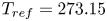 $T_{ref}=273.15$ K. The Rayleigh number can alternatively be interpreted as the ratio of convective to conductive velocity scales as
 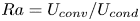 $Ra=U_{conv}/U_{cond}$ (Hewitt, Neufeld & Lister Reference Hewitt, Neufeld and Lister2013a,Reference Hewitt, Neufeld and Listerb), in which the convective velocity scale is
  $U_{conv}=\rho \beta \Delta T g K/\mu$ and the conductive velocity scale is
 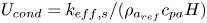 $U_{cond}=k_{{eff},s}/(\rho _{a_{ref}} c_{pa} H)$.
3. Numerical scheme, solution procedure and simulation set-ups
A direct numerical solver is developed to model the convection of water vapour with phase change in snowpacks. This new solver, named as  $\textit {snowpackBuoyantPimpleFoam}$, is based on the standard solver of
  $\textit {buoyantPimpleFoam}$ in the open-source fluid dynamics software OpenFOAM 5.0 (www.openfoam.org). Using a finite volume approach, the governing equations are discretized on a collocated grid. PIMPLE as a combined PISO-SIMPLE algorithm (Moukalled et al. Reference Moukalled2016) is used for the pressure–velocity coupling to solve the final set of equations described in § 2. For the solution procedure, the gas-phase velocity obtained by the momentum equation is used to solve the water vapour density and the temperature for the gas and ice phases. Then, the gas mixture continuity equation including the mass source (or sink) term along with the semi-discretized momentum equation are used to solve the resulting pressure Poisson equation to obtain continuity-satisfying velocity and pressure fields (Moukalled et al. Reference Moukalled2016). For the next time step, the heat and mass transfer coefficients are updated to repeat the solution procedure. To discretize the equations, the Gauss linear and Gauss linear corrected schemes, respectively, are used for the terms with gradient and divergence operations and the Euler scheme is chosen for the discretization of the transient terms (Moukalled et al. Reference Moukalled2016). The adjustable time step scheme with a limit on the Courant number was deployed to reduce the computational cost. The Courant number as the stability criterion is defined as
  $Co=|\left \langle \boldsymbol {U}_{g} \right \rangle | \Delta t/\Delta r$, where
  $\Delta t$ is the time step and
  $\Delta r$ is the distance between the computational cell centres.
The numerical simulation is performed for a natural convection flow in a two-dimensional snowpack of depth  $H$ and the length
  $L$. Figure 1 shows a sketch of the domain with the cyclic boundary conditions on lateral sides. The top and bottom boundaries are considered as impermeable walls with zero flux for the gas phase. For the heat transfer equations of both phases, the reference temperature is used as the bottom boundary condition,
  $T_{h}=T_{ref}$, whereas
  $T_{c}=T_{ref}-\Delta T$ is applied for the top boundary. The initial conditions are the reference temperature for both ice and gas phases and the saturation water vapour density as
  $\sigma =0$. A sensitivity analysis has shown that the results are not sensitive to the choice of initial temperature and vapour distribution (figure 23 in Appendix A). A non-uniform mesh in the vertical direction is used to ensure that the grid size is small enough of the order of
  $Ra^{-1}$ to resolve the thin boundary layers (Hewitt, Neufeld & Lister Reference Hewitt, Neufeld and Lister2014). Note that in reality snow settling will counteract the density decrease caused by convection to a certain extent and prevent very low densities at the bottom. Since snow settling is not simulated in our model, we artificially limited the density decrease by a threshold of 95 % for the porosity above which the phase change is stopped. In general, the convective–diffusive heat and mass transfer with phase change in snowpacks are very slow processes and changes are small enough at each time step to consider a quasi-steady-state process especially when the convection cells are completely formed and only show small lateral movement (see below). This is due to the fact that convection cells form and reach a quasi-steady state in the order of a few hours (shown later in figure 3), that the thermal boundary conditions are fixed and that the order of magnitude for the porosity change is small at each time step. Scaling analysis of the ice mass conservation shows that for the minimum Rayleigh number studied, and assuming maximum mass transfer potential of
  $\sigma =1$, the porosity change rate is small and of the order of
  $\partial \epsilon _{i}/\partial t \approx 10^{-9}$ s
 $^{-1}$. Hence, the convection–diffusion terms (the net vapour divergence for sublimation and convergence for deposition) are almost equal to the mass source/sink term. Thus, the maximum Courant number of 200 with the outer PIMPLE loop of 50 and residual control of
  $10^{-4}$ are used. Note that the sensitivity analysis performed shows that the results for the semi-steady-state process are not changing for the maximum Courant number less than 200 as shown in figures 24 and 25 in Appendix C. In addition, changing the domain length
  $L$ from 5 to 100 m did not change the results, as is shown in figure 26 in Appendix C. Hence, a domain length of 10 m was chosen for the simulations. The numerical set-up also was validated comparing with available numerical benchmarks in § 4. The thermal and physical properties of the gas and ice phases used in the present numerical simulations are listed in table 1.
A sketch of the two-dimensional domain with non-uniform mesh and prescribed boundary conditions.

The thermal and physical properties of the gas and ice phases evaluated at the reference temperature.
4. Numerical validation
The numerical benchmarks for natural convection in a square porous medium with hot and cold impermeable boundaries on the sides and adiabatic and impermeable boundaries on the top and bottom are used to examine the performance of the solver developed. First, the results obtained by the present model are compared against the cases of thermal equilibrium. To that end, the local and total Nusselt numbers adapted for the thermal equilibrium should be used (Saeid Reference Saeid2004):
 \begin{gather} Nu(z) = \frac{H}{\Delta T\left(\epsilon_{g}k_{{eff},g}+\epsilon_{i}k_{{eff},i}\right)} \left[ \epsilon_{g}k_{{eff},g} \frac{{\rm d} \left\langle T_{g} \right\rangle^{g}}{{\rm d}z}+\epsilon_{i}k_{{eff},i}\frac{{\rm d} \left\langle T_{i} \right\rangle^{i}}{{\rm d}z} \right], \end{gather}
 \begin{gather} \overline{Nu} = \frac{1}{H}\int_{0}^{H} Nu(z)\, {\rm d}z. \end{gather}
 Figure 2 shows the transient variation of the local Nusselt number with scaled time  $\tau =k_{{eff},s}t/\left (\left (\epsilon _{g} \rho _{a_{ref}} c_{pa} + \epsilon _{i} \rho _{i} c_{pi}\right ) H^{2}\right )$ for
  $Ra=100$. The grid dependency analysis shows that the temporal variation of
  $Nu$ for the heights in the middle and upper parts of the domain does not change with increasing grid size and mostly the error is less than 5 % while increasing the spatial resolution helps to decrease the error for the bottom region of the domain. However, in general, a good agreement between the present model and the numerical benchmark by Saeid & Pop (Reference Saeid and Pop2004) can be seen for the transient behaviour of the local heat transfer. In table 2, the resulting total Nusselt numbers for different Rayleigh numbers are compared with some available numerical benchmarks to verify the performance of the present solver. The larger variations of
  $Nu$ between different studies for higher
  $Ra$ are due to unstable and chaotic behaviour of the flow which requires fine resolution dependent on
  $Ra$ as discussed in § 3.
Comparison of the present results with the numerical benchmark by Saeid & Pop (Reference Saeid and Pop2004) (a) for the transient variation of the local Nusselt number with scaled time  $\tau$ at three non-dimensional heights for
  $Ra=100$ and (b) the relative error for different grid sizes.

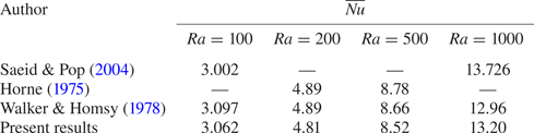
Comparison of the total Nusselt number  $\overline {Nu}$ defined in (4.1b) at steady state with some previous numerical benchmarks.
Finally, a comparison was done with the results of local thermal non-equilibrium model by Baytas & Pop (Reference Baytas and Pop2002) using the total Nusselt number defined separately for the gas and ice phases at cold and hot surfaces of the cavity as
 \begin{gather} \overline{Nu_{g}} = \frac{1}{\Delta T} \int_{0}^{H} \frac{{\rm d} \left\langle T_{g} \right\rangle^{g}}{{\rm d}z} \,{\rm d}z, \end{gather}
 \begin{gather} \overline{Nu_{i}} = \frac{1}{\Delta T} \int_{0}^{H} \frac{{\rm d} \left\langle T_{i} \right\rangle^{i}}{{\rm d}z}\,{\rm d}z. \end{gather}
 Note that we have used the same term for the heat transfer between two phases as presented in Baytas & Pop (Reference Baytas and Pop2002). From comparing the results in table 3, we found that the present results for  $\overline {Nu_{i}}$ are very close to the numerical benchmark and that the maximum error for
  $\overline {Nu_{g}}$ compared with the benchmark is less than 3 %.
Comparison of the total Nusselt numbers  $\overline {Nu_{g}}$ and
  $\overline {Nu_{i}}$ for the case of local thermal non-equilibrium model with fixed Rayleigh number
  $Ra=500$ and
  $k_{{eff},g}=k_{{eff},i}$ but different heat transfer coefficients
  $h_{c}$.

5. Results and discussion
To the best of our knowledge, we explore for the first time the convection of water vapour in a phase-changing snowpack and its effects on snow density change by looking at the thermal and phase change regimes for different snowpack conditions (vertical size, thermal boundary conditions, Rayleigh number). The conductive and convective velocity scales introduced in § 2.3 are the key measures to analyse the thermal and mass transfer in a snowpack and they are needed to show the differences in the phase change regime for different snowpack conditions. As the effective thermal conductivity and the intrinsic permeability of snow given respectively by (2.20) and (2.9) both are a function of porosity, for a specified Rayleigh number, the two parameters of interest are the snow height and the temperature difference (as the thermal boundary conditions) which define the conductive and convective velocity scales and are discussed separately later.
In order to provide a context for our results, we summarize the main observations first. In § 5.1, the general thermal and phase change behaviour in the snowpack is discussed and we find that (1) the thermal and phase change pattern in a convection cell is qualitatively the same in all different snowpacks, (2) there is considerable impact of natural convection on the snow density distribution with a layer of significantly lower density at the bottom of the snowpack and a layer of higher density located at the top and (3) as discussed in § 5.2, the horizontal displacement of the convection cells leads to a wider area of the top and bottom region to experience phase change processes, resulting in an almost uniformly increased snow density on the top mirroring the reduced density in the bottom region. Quantitatively, different phase change rates in snowpacks with various conditions (vertical size, thermal boundary conditions, Rayleigh number) are caused by the difference in the thermal and the flow regimes between their respective deposition and sublimation zones. In this respect, the heat and mass transfer are compared between different snow heights  $H$ in § 5.3 while the effect of the temperature difference
  $\Delta T$ is investigated in § 5.4.
5.1. General thermal and phase change behaviour
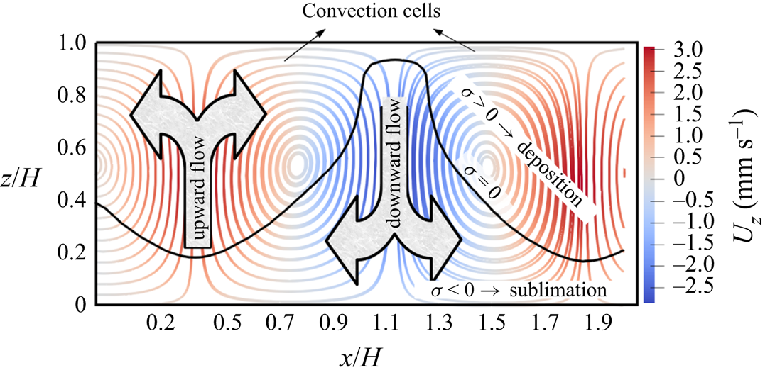
When the Rayleigh number is large enough such that convection cells form, the regime generally develops through three stages: (1) the pure conduction mode, (2) the transition mode when convection cells start to form and (3) the predominant convection mode when the convection cells are completely formed. As an example, figure 3 shows the evolution of the thermal regime through different stages, indicating also the flow directions. Both conduction heat transfer rate and the Rayleigh number determine how long stages 1 and 2 last. In figure 3(a) conduction is still the dominant mode. As the initial temperature is uniform and equal to the bottom warm boundary, at the start of simulation, there is considerable conduction heat transfer in the region close to the top boundary, cooling down that region (stage 1 of the thermal regime). While the conduction leads to cooling of the bottom region, the convection starts to be active on the top region. This is shown in figure 3(b) as stage 2 of the thermal regime. Figure 3(c) shows the transition between stages 2 and 3 when the convection cells fill almost the whole domain but they are not yet completely formed and stable. Finally, the convection mode with completely formed convection cells is shown in figure 3(d) as the last stage of the regime development. Figure 4 indicates the completely formed convection cells by streamlines. As shown in this figure, each convection cell is formed by neighbouring upward and downward flows. Also, these cells can be split by the saturation line  $\sigma =0$ into the deposition zone (above the saturation line) and sublimation zone (below the saturation line).
Evolution of the thermal regime through different stages. (a) The pure conduction mode at time = 1 h, (b) transition mode when the convection starts to form on top at time = 6 h, (c) transition mode when the convection cells fill almost the whole domain but not completely formed and stable at time = 12 h and (d) the predominant convection mode with completely formed convection cells at time = 22 h with maximum gas velocity of  $3.1 \times 10^{-3}$ m s
 $^{-1}$. The white arrows show the flow direction scaled by velocity magnitude. The black line refers to the saturation line where
  $\sigma =0$. The isotherm lines for the snow temperature are in blue which are equally spaced by 5 K.
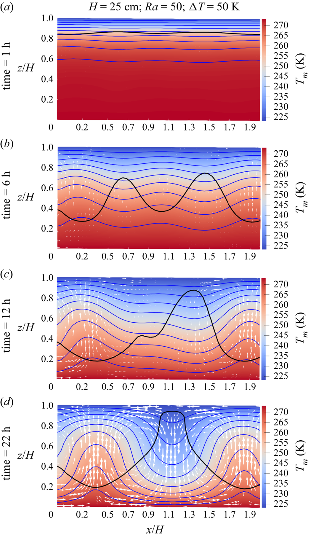
Streamlines for the completely formed convection cells. The black line refers to the saturation line  $\sigma =0$, above and below which are the deposition and sublimation zones respectively.
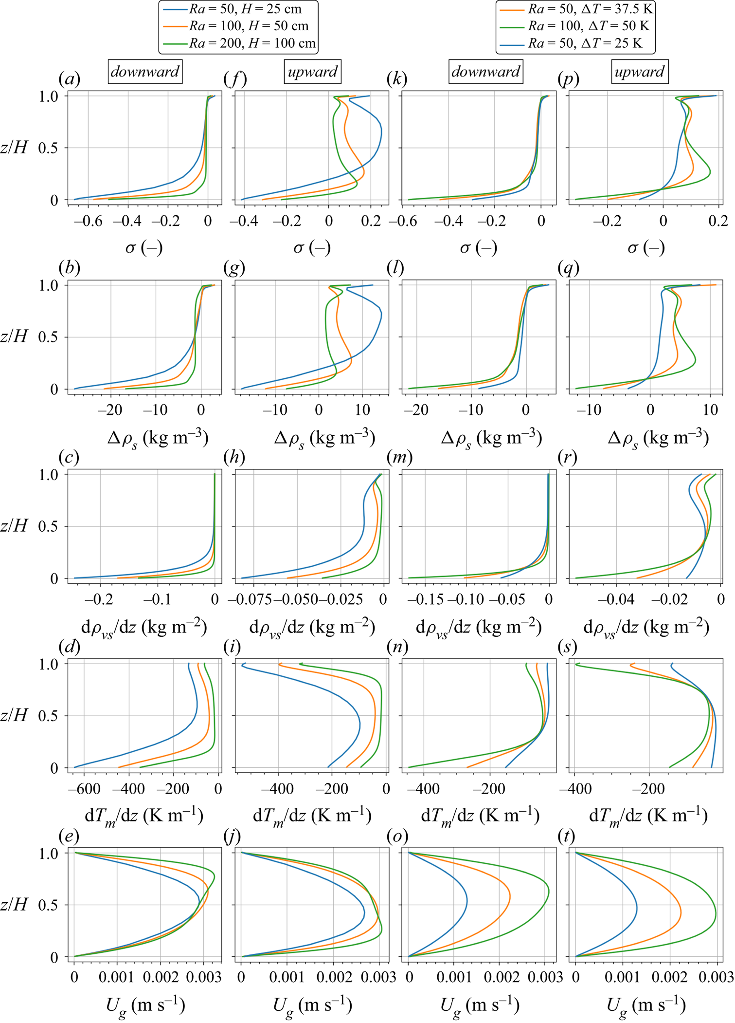
It should be noted that the general thermal and phase change behaviours in the upward and downward flows of a convection cell are qualitatively the same for snowpacks with different conditions (e.g. snow height, thermal boundary conditions, Rayleigh number). Hence, we analyse the heat and mass transfer regimes in different parts of a chosen convection cell after one week of the simulation for a sample case with snow height  $H=25$ cm, temperature difference
  $\Delta T=50$ K and
  $Ra=50$. Figure 5 shows profiles for the saturation degree, snow density change, saturation vapour density gradient, snow temperature gradient and the air flow velocity in the upward and downward flows of a convection cell for two scenarios, i.e different snow heights and different temperature boundary conditions. Also, two-dimensional plots of the chosen convection cell for the sample case (snow height
  $H=25$ cm, temperature difference
  $\Delta T=50$ K and
  $Ra=50$) are shown in figure 6. In these two-dimensional plots, to highlight downward flows, the marker points p7, p1, p2 and p3 are used, while for the upward flows the markers p4, p5 and p6 are used. In general, when convection is active, the downward convective flow stretches the top cold temperature towards the bottom hot boundary. As shown in figure 5(a,n), this causes a smaller temperature gradient on top and larger temperature gradient in the bottom region. Oppositely, the upward convective flow stretches the bottom warm temperature towards the top resulting in a smaller temperature gradient at the bottom region and a larger gradient on the top because of the fixed top boundary temperature (figure 5i,s). Thus, compared with the pure conduction temperature profile, the region is colder in downward flow and warmer in upward flow. Also, in both upward and downward flows, the maximum stretching (the smallest temperature gradient) occurs where the gas flow velocity reaches maximum (compare figure 5n,o). For both regions close to and far enough from the boundaries, it is discussed later that the effect of the convective stretching on the temperature profile in different snowpacks is determined by the Rayleigh number.
One-dimensional profiles of the saturation degree  $\sigma$, the snow density change
  $\Delta \rho _{s}$, the gradient of saturation vapour density
  ${\rm d}\rho _{vs}/{\rm d}z$, the snow temperature gradient
  ${\rm d}T_{m}/{\rm d}z$ and the gas flow velocity
  $U_{g}$ at the location of downward and upward flows of a convection cell for different snow heights
  $H$ and temperature difference
  $\Delta T$.
Simulated two-dimensional plots for the sample case with snow height  $H=25\,{\rm cm}$, temperature difference
  $\Delta T=50\,{\rm K}$ and
  $Ra=50$. (a) The saturation degree
  $\sigma$, (b) the snow density change
  $\Delta \rho _{s}/\rho _{so}$, (c) the water vapour density
  $\rho ^{*}_{v}=\left \langle \rho _{v} \right \rangle ^{g}/\rho _{vs_{ref}}$ and (d) the diffusive water vapour flux
  $J^{*}_{v}=\left \langle J_{v} \right \rangle /(D_{va} \rho _{vs_{ref}}/H)$. The black line refers to the saturation line where
  $\sigma =0$. The isotherm lines for the snow temperature are in blue which are equally spaced by 5 K.
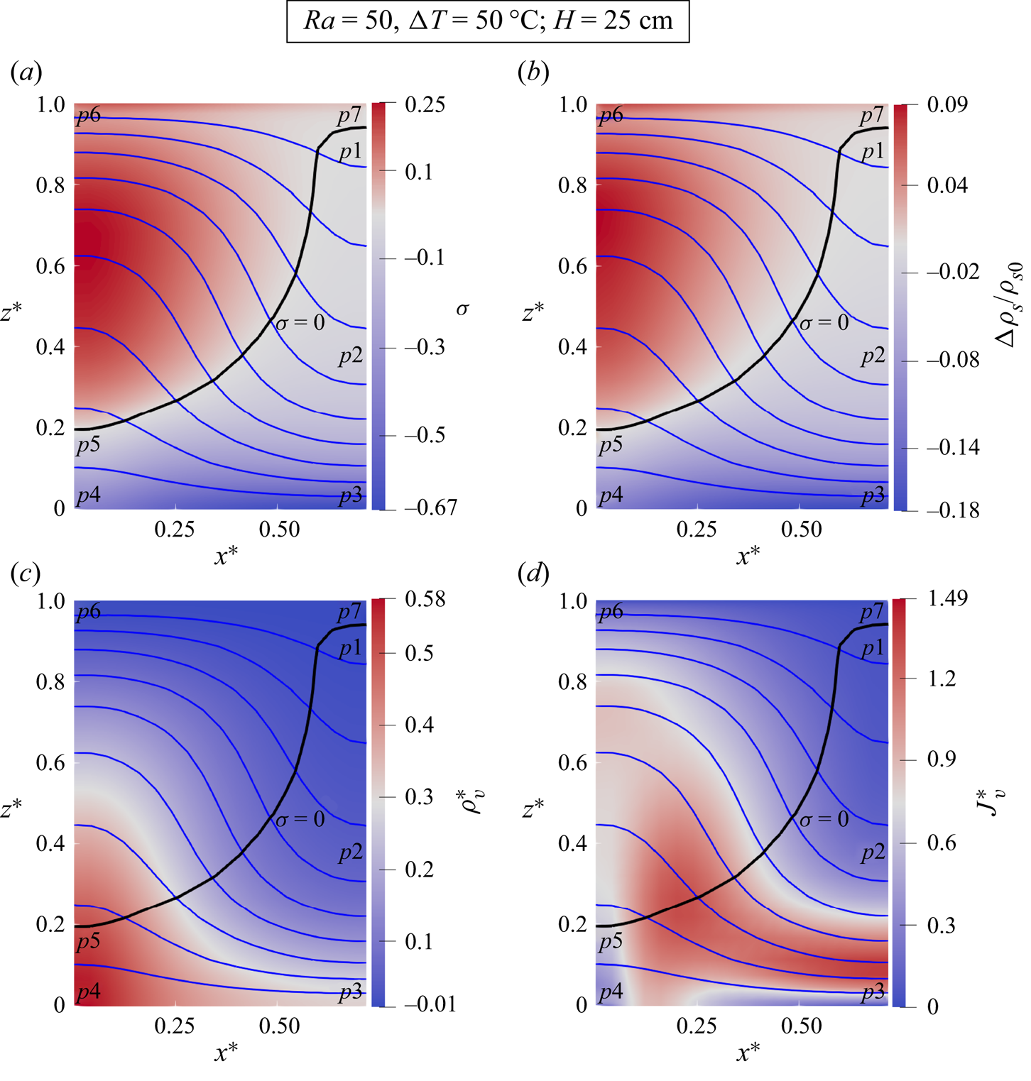
For the phase change regime in different parts of a chosen convection cell, we first analyse the downward flow from the saturation line. While the downward convective flow transports the water vapour towards the bottom (leading to less vapour content and smaller vapour gradient in the upper part), the sublimation phase change simultaneously counteracts the convection effect by adding vapour to the upper part. As discussed in Appendix D, the phase change rate is dependent on both the convective flow rate and the gradient of the saturation vapour density. With almost a constant convective flow velocity, the phase change rate mainly reacts on the saturation vapour density gradient, which itself is related to the temperature and temperature gradient,  ${\rm d}\rho _{v,s}/{\rm d}z \propto \rho _{v,s} \times {\rm d}T/{\rm d}z$. In this respect, the sublimation zone is not vertically uniform in downward flow and may be split into three parts:
(i) For the cold region between p1 and p2, both temperature and its gradient are much smaller compared with the bottom region, resulting in much smaller phase change rate and thus a smaller value for oversaturation
 $\sigma$ just around $-0.05$ as shown in figure 6(a).
(ii) The warmer region between p2 and p3, with a much larger temperature and temperature gradient than the first region (figure 5d), has a much larger sublimation rate as shown for the oversaturation
$\sigma$ in figure 5(a) and for the snow density change $\Delta \rho _{s}$ in figure 5(b). Also, it should be noted that the downward convective flow towards the bottom zero-flux boundary and also the large sublimation rate in the bottom region both cause a local concentration of the water vapour to increase the vapour density gradient. This is the reason for the larger upward diffusive flux in the bottom region as shown in figure 6(d).(iii) In the horizontal flow of the bottom region, from p2 and p3 to p4 and p5, the sublimation rate (represented by the saturation degree
$\sigma$ and also the snow density change $\Delta \rho _{s}$ in figure 6) decreases as the saturation vapour density gradient decreases along with the temperature gradient. This can be seen by comparing the panels of figure 5 at the bottom region between the downward and upward flows. It should be noted that the bottom region between p4 and p5 has the highest water vapour content shown in figure 6(c). This is a result of flow advection and local sublimation.


Similarly, the phase change regime for the upward flow of the chosen convection cell is analysed as follows:
(i) In the bottom region between p4 and p5, the convective flow transports and concentrates the vapour content upward, trying to reduce the vapour content and magnitude of its gradient in upstream flow, while the sublimation counteracts the convection effect by adding vapour content to upstream flow, causing a more linear vapour profile.
(ii) In the deposition zone between p5 and p6, the effect of the upward flow is to transport all the vapour towards the top, making the upstream flow devoid of vapour. But, this time, the deposition process counteracts the convection effect by removing water vapour from the upstream flow as can be seen from comparing the water vapour content shown in figure 6(c). Finally, the opposite effects of the upward convection and deposition processes form an almost linear vapour profile with a negative slope. It should be noted that for the region close to the top boundary, because of the zero-flux boundary conditions, there is still a slight vapour density gradient and this causes an upward diffusive flux slightly larger in that region compared with the upstream flow in the middle of the domain (shown in figure 6d).
(iii) In the horizontal flow on the top region, as the flow goes from p6 to p7 and p1, the saturation vapour density gradient decreases because both temperature and temperature gradient decrease, along with the fact that the magnitude of saturation degree decreases. This can be seen by comparing the panels of figure 5. The deposition region of the downward flow has the minimum phase change rate (looking at figure 5(a) for the saturation degree
$\sigma$ and also figure 5(b) for the snow density change $\Delta \rho _{s}$) due to the minimum saturation vapour density gradient in the convection cell shown in figure 5(c). As the water vapour of the neighbouring upward flows is constantly consumed to reach the deposition zone in the downward flow, this region has the lowest vapour content as shown in figure 6(c).


We compare the deposition zone between p5 and p6 with the sublimation zone at the same non-dimensional heights. While both regions have more or less the same temperature gradient except for the regions close to the boundaries (comparing figure 5d with 5i), the deposition zone has a larger saturation vapour density gradient (comparing figure 5c with 5h) because of its higher temperature. This results in a larger magnitude for the phase change rate (comparing figure 5b with 5g), the saturation degree (comparing figure 5a with 5f) and the saturation degree gradient in the deposition zone. However, compared to the bottom sublimation zone between p2 and p3, both the temperature and its gradient in the deposition zone between p5 and p6 are much smaller. Thus, the phase change rate is higher in the sublimation zone. As shown in figure 6(a) for the saturation degree and also in figure 6(b) for the snow density change, this is the reason why there is a vertical effective deposition zone with a smaller saturation degree less than around 0.2 while the effective sublimation zone is horizontal in the bottom region with saturation degree ranging from  $-0.05$ to
  $-0.9$.
5.2. Horizontal displacement of convection cells
In natural convection without phase change in the porous medium, and with moderate Rayleigh number, the convection cells are fixed and are not moving horizontally in the domain. This is not the case when there is phase change and therefore density and porosity changes in the snowpack. This is because the convection cells induce heterogeneity in the snow porosity due to spatially varying phase change, which causes the momentum to be horizontally imbalanced. This temporary imbalance in momentum causes a displacement of the convection cells until the momentum again reaches a stable and balanced condition. The local phase change rate determines how fast the induced heterogeneity of the porosity grows in the domain and also how many times the horizontal displacement of the convection cell occurs during the snowpack life time. From what we observed numerically in different snowpacks, the displacement of the convection cells is large enough (of the order of a convection cell and snowpack height) to change locally the sign of both the phase change rate and the flow direction. For instance, a region which was already under the deposition process of an upward flow transforms into a region undergoing sublimation with a downward flow. For different snow heights, the convection cell displacements at four different time snapshots are shown in figure 7. At the first time snapshot, i.e. after a week of the simulation (figure 7a,e,i), a grey column is used between two neighbour cells as a fixed reference position to compare the cell displacement between time snapshots. Considering the phase change pattern analysed for a convection cell in § 5.1, the effects of the convection cell displacement are discussed as follows.
Simulated two-dimensional plots after a week of simulation for (a,e,i) the saturation degree  $\sigma$, (b,f,j) the snow density change
  $\Delta \rho _{s}/\rho _{so}$, (c,g,k) the water vapour density
  $\rho ^{*}_{v}=\left \langle \rho _{v} \right \rangle ^{g}/\rho _{vs_{ref}}$ and (d,h,l) the diffusive water vapour flux
  $J^{*}_{v}=\left \langle J_{v} \right \rangle /(D_{va} \rho _{vs_{ref}}/H)$ for three snow heights
  $H=25\,{\rm cm}\ (Ra=50)$,
  $H=50\,{\rm cm}\ (Ra=100)$ and
  $H=100\,{\rm cm}\ (Ra=200)$. The black line refers to the saturation line where
  $\sigma =0$. The isotherm lines for the snow temperature are in blue which are equally spaced by 5 K.

The region which was already under an upward flow: (i) the top region of the increased snow density, after the convection cell displacement, becomes the sublimation zone of a downward flow. As already discussed, the sublimation rate in this region is very small so that it barely reduces the snow density. (ii) The bottom region of the decreased snow density switches to sublimation in a downward flow which has the strongest phase change rate in a convection cell. This reduces the snow density of this region more than before. The region which was already in a downward flow: (i) the bottom region of the decreased snow density now becomes the sublimation zone of an upward flow. Still, the snow density in this region decreases but at a smaller rate than before. (ii) The top region of the almost constant snow density goes under the deposition zone of an upward flow. Obviously, the snow density increases in this region.
The conclusion of these four points is that the lateral displacement of the convection cells leads overall to an almost uniform higher snow density close to the surface and lower snow density at the bottom for the assumed temperature gradient of warmer temperatures at the bottom, which is the usual case in seasonal snow and on sea ice.
5.3. Effect of snow height, $H$

The three snowpack heights investigated in this section are of small ( $H=25\,{\rm cm}$ and
  $Ra=50$), medium (
 $H=50\,{\rm cm}$ and
  $Ra=100$) and large (
 $H=100\,{\rm cm}$ and
  $Ra=200$) sizes. With the same initial porosity
  $\epsilon _{g}=0.8335$, bottom thermal boundary condition of
  $T=273.15\,{\rm K}$ and temperature difference
  $\Delta T=50\,{\rm K}$, the convective velocity scale
  $U_{conv}=\rho \beta \Delta T g K/\mu$ is the same for all snow heights while the conductive velocity scale
  $U_{cond}=k_{{eff},s}/(\rho _{a_{ref}} c_{pa} H)$ is different and smaller for the larger snowpack. To analyse the snow height effects on the convective vapour transport, we want to compare the temperature and its gradient, representing directly the saturation vapour density gradient as the main reason for the different phase change rates in snowpacks with the same convective flow velocity scales. The difference in the temperature and temperature gradient profiles between different snow heights is qualitatively discussed as follows.
(i) For the regions close to the boundaries, represented by the marker points p4, p6, p7 and p3 in figure 7: the small snowpack has the largest conductive velocity scale resulting in a more linear temperature profile and smaller temperature gradient with respect to the non-dimensional snow height
$z^{*}=z/H$ (comparing the blue isothermal lines in all panels of figure 7). However, in these regions, the smaller snowpack has a larger temperature gradient with respect to the dimensional height (${\rm d}T/{\rm d}z=1/H \times {\rm d}T/{\rm d}z^{*}$) and thus, as shown in figure 5(d), ${\rm d}T/{\rm d}z|_{H=25\,cm}>{\rm d}T/{\rm d}z|_{H=50\,cm}>{\rm d}T/{\rm d}z|_{H=100\,cm}$.(ii) The sublimation zone in the downward flow between markers p1 and p2 in figure 7: for the larger snowpack, the conductive velocity scale is smaller and it has, therefore, a smaller effect against the convective heat transfer. Hence, the convective stretching effect on the temperature profile is stronger, resulting in a smaller – and overall less linear – temperature gradient with respect to both non-dimensional (comparing the blue isothermal lines in all panels of figure 7) and dimensional (comparing three plots in figure 5d) heights. This is the reason for a larger region with smaller saturation vapour density gradient (figure 5c) and thus phase change rate (represented by snow density change in figure 5b). Note that this also refers to a smaller area between markers p2 and p3 (p3 is located where
$|\sigma =5\,\%|$) where the phase change rate is significant. In other words, the larger the snowpack, the smaller the area in which the saturation degree magnitude is greater than 5 %, meaning that it has a smaller significant sublimation area in percentage compared with the smaller snowpacks (comparing the area size between p2 and p3 shown in all panels of figure 7).(iii) The deposition zone in the upward flow between markers p5 and p6 in figure 7: first, it should be noted that even though the larger snowpack has a smaller and less significant sublimation area, due to its larger size, it has cumulatively more water vapour accumulated in the region between p4 and p5 (comparing the maximum value for the water vapour density in figure 7c,g,k). This moves the saturation line (black line where
$\sigma =0$) closer to the bottom boundary for the larger snowpack, causing the sublimation zone between markers p4 and p5 to be smaller in a relative sense. For the deposition region above the marker p5 and far from the top boundary, the small snowpack has both a more linear temperature profile and thus a more uniform temperature gradient because of its reduced stretching (comparing the blue isothermal lines in all panels of figure 7). This causes a more uniform saturation degree and phase change rate than for the larger snowpacks. On the contrary, the large snowpack has two peaks in saturation degree with an almost saturated area in between (figure 7i). Its first peak is located in the lower half of the domain while the second one is located close to the top boundary. For the medium snowpack shown in figure 7(e), the distance between these peaks is smaller, meaning that it has a smaller area of almost zero saturation degree compared with the large snowpack.


As introduced in § 5.2, convection cells move laterally due to changes in porosity distribution (induced heterogeneity) and its feedback on the flow. The process of breaking the symmetry in the system is first a continuous process responding to higher local phase change rate and then it relaxes to a steady state with a decreasing lateral movement of convection cells. A plausible explanation for these two stages is given as follows.
To support our hypothesis, the magnitude of different terms in the momentum equation as well as the flow velocity are shown in figure 8 for 18 days before the onset of lateral movement of convection cells. We follow a path between the marker points p1 and p7 (figure 3) first up, then right, then down and finally left within the cell. For the top region in the upward flow, comparing the case with phase change with the same case without phase change, the intrinsic permeability decreases exponentially with an increase in snow density (2.9) leading to a higher viscous resistance factor, i.e.  $\mu /K$, while the viscous resistance force itself is almost unaltered (figure 8b for upward flow). This increased resistance factor causes a reduced flow velocity of approximately 25 % before lateral movement of convection cells begins (figure 8d for upward flow). The reduced flow velocity has a direct feedback on the temperature gradient and thus both gas density gradient and dynamic pressure gradient forces are decreased also by 25 % (figure 8a,c for upward and top-right flow). At the bottom, reduced density causes almost 100 % velocity increase (figure 8d for bottom-left flow). The flow-blocking effect in upward flow (deposition zone) counteracts the significantly increased flow velocity at the bottom. The former tends to counteract the convection, while the latter tries to keep the convection cell at its location. However, for the lateral displacement of convection cells, this partially stable system needs a disturbance in the momentum (spatiotemporal chaos (Egolf et al. Reference Egolf, Melnikov, Pesch and Ecke2000)). The flow changes the path towards the lower-density section on the top next to the initial deposition zone. This finally leads to the intuitive result that cells move laterally to avoid regions of higher density. The displacement decreases over time and a new symmetry in density distribution is established.
The magnitude of each term in momentum equation (2.8) as well as the flow velocity for 18 days before lateral movement of convection cells along the path of a convection cell. Using the marker points introduced in § 5.1: upward flow between markers p4 and p6, top-right flow between markers p6 and p7, downward flow between markers p7 and p3 and bottom-left flow between markers p3 and p4.

To indicate temporal variations in lateral displacement of convection cells through the two stages explained above, the time series of temperature for some fixed points are used as  $T(t,\boldsymbol {r}_{fp})$. These fixed points with position
  $\boldsymbol {r}_{fp}$ are located on the peak of temperature
  $(T_c+T_h)/2$ (in the upward flow) for all convection cells formed in the system (the initial temperature is
  $(T_c+T_h)/2$). As the convection cells move laterally, the temperatures probed by these fixed points decrease, indicating how fast and large the cells are moving through phases 1 and 2. The average of these temperatures over all fixed points,
  $\bar {T}=\sum ^{} T(t,\boldsymbol {r}_{fp})/N_{fp}$, is shown in figure 9. As shown in these plots, the smaller the snowpack, the faster the transition from stage 1 to stage 2 (from a continuous and persistent drift to a steady state with negligible convection cell movement) because of its larger snow density change. One more interesting point that we found only for the small snowpack is that the convection cell size increases in accordance with stage 1 of convection cell movement (figure 10). From what we observed, during stage 1 of the cell displacement, the neighbouring convection cells are merging leading to larger averaged cell sizes. This is because the convection cells are not moving laterally with the same rate direction. Each step change in the cell size for the small snowpack (figure 10) corresponds to merging a pair of neighbouring cells. For a medium snowpack, after a period of slow displacement of convection cells, we observe a sudden change in
  $\bar {T}$, meaning a fast transition from stage 1 to stage 2. For the larger snowpack, it has only a much longer stage 1 and its transition to stage 2 such that the convection cell keeps slowly moving without reaching a complete new steady state and symmetry in porosity distribution.
Temporal variations in lateral displacement of convection cells using the averaged probed temperature  $\bar {T}$ as discussed in § 5.2 for different snow heights.

Comparison of the normalized convection cell size for different domain width for the case with phase change.

For the range of moderate Rayleigh numbers when we have stable convection cells (Caltagirone Reference Caltagirone1975), the number of convection cells and the average cell size are directly related to the Rayleigh number such that the higher the Rayleigh number, the more slender are the cells formed in the domain (Holzbecher Reference Holzbecher2019) as shown in figure 27 in Appendix C. The sensitivity analysis shows the domain width has a small effect on the averaged cell size for the case without phase change. For the case with phase change, the convection cell size has more variation on changing the domain width (figure 28 in Appendix C). However, the laterally averaged snow density change is statistically the same and independent of the domain width as shown in figure 26 in Appendix C. It should be noted that the cell size is calculated as the distance between the maximum of the temperature level in upward flow and its minimum in the downward flow of a convection cell. Accordingly, the initial cell size after a week of simulation for the small, medium and large snowpacks is around  $0.7H$,
  $0.4H$ and
  $0.3H$ as shown in figure 11(a,e,i). Given the fact discussed earlier that the small snowpack has a larger relative size (or extent) for the sublimation and deposition zones which are stronger than for the larger snowpacks, the induced heterogeneity occurs faster and earlier such that the initial convection cell (formed after a week shown in figure 11a) moves laterally around
  $0.8H$ during the first month of the simulation (comparing figures 11b and 11a). The horizontal displacement is approximately 14 % greater than the initial cell size. For the medium snowpack during the first month, the convection cell moves laterally only around
  $0.15H$ (37.5 % of its initial convection cell from comparing figures 11e and 11f). During the second month of the simulation, the small snowpack reaches an almost stable horizontal porosity distribution to have a small convection cell displacement around
  $0.1H$ (figure 11c compared to figure 11b) and also the convection cells are almost fixed until the end of the simulation (figure 11d compared to figure 11c). This is different for the medium snowpack as the induced heterogeneity gets large enough during the second month to trigger a significant displacement of around
  $0.6H$ (comparing figures 11g and 11f). Note that the convection cells are almost stable and fixed for the rest of the simulation (figure 11h compared with figure 11g). The large snowpack has the smallest and slowest convection cell displacement because of its smaller and less significant phase change area (non-dimensional size) compared to the small and medium snowpacks. It has almost the same displacement around
  $0.05H$ during both the first and second month of the simulation (comparing figures 11i, 11j, 11k and 11l).
Simulated two-dimensional plots for snow density change  $\Delta \rho _{s}$, showing the the horizontal displacement of the convection cells at four time snapshots for different snow heights. The grey column is used as the reference to measure the horizontal displacement between the different time snapshots. The black line refers to saturation line where
  $\sigma =0$. The isotherm lines for the snow temperature are in blue which are equally spaced by 5 K.

For a general comparison of convective water vapour transport between different snow heights, the time series of snow density change, standard deviation of snow density change, snow temperature and saturation degree are shown in figure 12 based on a lateral average for each level of  $z$. The non-dimensional thickness of the low-density ‘weak layer’ at the bottom of the snowpack, which has the minimum possible density (based on the threshold of 95 % set for the porosity above which the phase change is stopped) is around
  $0.2H$,
  $0.1H$ and
  $0.05H$ for small, medium and large snowpacks respectively. It takes 5, 7 and 11 weeks to reach for the first time the minimum snow density at the bottom for the small, medium and large snowpacks respectively. The small snowpack has a pronounced density change on top for which 46 % of its top region experienced a density increase of more than 25 %. However, only approximately 30 % and 10 % of the top region experienced a density increase of more than 25 % for the medium and large snowpacks, respectively. The maximum increase in density on top is 57 % (87 kg m
 $^{-3}$), 47 % (72 kg m
 $^{-3}$) and 29 % (45 kg m
 $^{-3}$) for small, medium and large snowpacks respectively. It is shown in figure 11(d) that through the upward flow within convection cells, a patch with minimum possible density (MPD patch) is formed in the weak layer. Such MPD patches are larger for the small snowpacks such that their vertical size may reach
  $0.5H$. As discussed earlier, this is due to the larger sublimation rate for the small snowpack such that the weak layer at the bottom forms faster and it gets thicker at the end of the simulation compared with the larger snowpacks. For the same reason, the small snowpack has the largest standard deviation of snow density change, which amounts to approximately 70 kg m
 $^{-3}$, while it is around 50 and 40 kg m
 $^{-3}$ for the medium and large snowpacks respectively.
The time series of (a–c) snow density change  $\Delta \rho _{s}$ and (d–f) the standard deviation of snow density change
  $\rho _{s,std}$ for different snow heights.

5.4. Effect of the temperature difference, $\Delta T$

Setting the same initial porosity  $\epsilon _{g}=0.8335$, bottom thermal boundary condition of
  $T=273.15\,{\rm K}$ and snow height of
  $H=50\,{\rm cm}$, three cases with different temperature differences are investigated in this section: the case of high
  $Ra$ (
 $\Delta T=50,\,Ra=100$), medium
  $Ra$ (
 $\Delta T=37.15,\,Ra=75$) and the low
  $Ra$ (
 $\Delta T=25,\,Ra=50$). In contrast to the previous section, here, the conductive velocity scale is almost the same in all cases while a larger
  $\Delta T$ (higher
  $Ra$) leads to a larger convective velocity scale. Thus, both the saturation vapour density gradient and the convective flow velocity should be considered simultaneously when analysing the difference in the snow density change:
(i) In the downward flow, the region from the top boundary to the non-dimensional height level of
$z^{*}=0.25$: even though the larger $\Delta T$ and $Ra$ favours more convective stretching and a smaller temperature gradient, the larger $\Delta T$ over the same snow height dominates to cause a larger temperature gradient (comparing three plots in figure 5n). Also, it is colder than the other cases with a smaller saturation vapour density gradient (figure 5m). Comparing the case of highest $Ra=100$ with lowest $Ra=50$, we found that the highest $Ra$ has a larger snow density change as its convective flow velocity is higher (figure 5o). Moreover, the difference in the snow density changes between the two cases gets larger as the flow penetrates further down since the convective flow increases in strength. However, for the case of medium $Ra=75$, the effect of the larger saturation density gradient compensates the effect of its lower convective flow velocity to have more or less the same snow density change compared with the case of higher $Ra$.(ii) In the downward flow, the region close to the bottom boundary: the case of higher
$Ra$ has a larger snow density change (figure 5l) because of its stronger saturation density gradient (figure 5m) and higher convective flow velocity (figure 5o). Note that the larger convective temperature stretching and also the larger $\Delta T$ within the same snow height both lead to a stronger saturation vapour density gradient for the case of higher $Ra$.(iii) In the upward flow, the region from the top boundary to the non-dimensional height level of
$z^{*}=0.25$: similar to what was previously analysed for the downward flow, even with a larger temperature gradient (figure 5s), the case of higher $Ra$ has a smaller saturation vapour density gradient (figure 5r) as it is colder in this region. However, its higher convective flow velocity causes a larger snow density change and saturation degree compared with the lowest $Ra$ case. Comparing with the medium $Ra$ case, the case of high $Ra$ has almost the same snow density change in the upper half of the domain while a larger snow density change in the lower half of the domain (figure 5q). This is because in the lower half of the domain, both the convective flow velocity (figure 5t) and the saturation vapour density gradient are larger in the high-$Ra$ case.(iv) In the upward flow, the region close to the bottom boundary: for the case of higher
$Ra$, the larger temperature gradient because of larger $\Delta T$ over the same snow height and thus the stronger saturation vapour density gradient and also higher convective flow velocity all cause a larger snow density change compared with the lower-$Ra$ cases.


The convection displacements at four different time snapshots are shown in figure 13. During the first month of the simulation, by comparing figure 13(b) with figure 13(a) for the low- $Ra$ case and also figure 13(e) with figure 13(f) for the medium-
 $Ra$ case, we found that for both low- and medium-
 $Ra$ cases, no convection displacement is observed while the case of high
  $Ra$ experiences a displacement of around
  $0.2H$ because of its larger snow density change (larger heterogeneity) at the bottom and middle of the snowpack (comparing figure 13j with figure 13i). During the second month of the simulation, the low-
 $Ra$ case still has almost no convection displacement (figure 13c compared with figure 13b) while the medium-
 $Ra$ case has a large enough heterogeneity in the snow density to have a displacement of around
  $0.2H$ (figure 13g compared to figure 13f). In this period, for the case of high
  $Ra$, the convection displacement of the cells gets even larger than during the first month (figure 13k compared with figure 13j) and the cells are almost fixed until the end of the simulation (figure 13l compared with figure 13k). For the cases of low and medium
  $Ra$, large enough heterogeneity in the snow porosity is only achieved during the last four months of the simulation and triggers a significant convection cell displacement (comparing figure 13d with figure 13c for the low-
 $Ra$ case and also figure 13h with figure 13g for the medium-
 $Ra$ case). Obviously, this is faster for the case of medium
  $Ra$ as its snow density change due to convective vapour transport is stronger than the case of low
  $Ra$.
$Ra$.
Simulated two-dimensional plots for snow density change  $\Delta \rho _{s}$, showing the horizontal displacement of the convection cells at four time snapshots for three temperature differences of
  $\Delta T=25\,{\rm K}\ (Ra=50)$,
  $\Delta T=37.5\,{\rm K}\ (Ra=75)$ and
  $\Delta T=50\,{\rm K}\ (Ra=100)$. The grey column is used as the reference to measure the horizontal displacement between the different time snapshots. The black line refers to the saturation line where
  $\sigma =0$. The isotherm lines for the snow temperature are in blue which are equally spaced by 5 K.
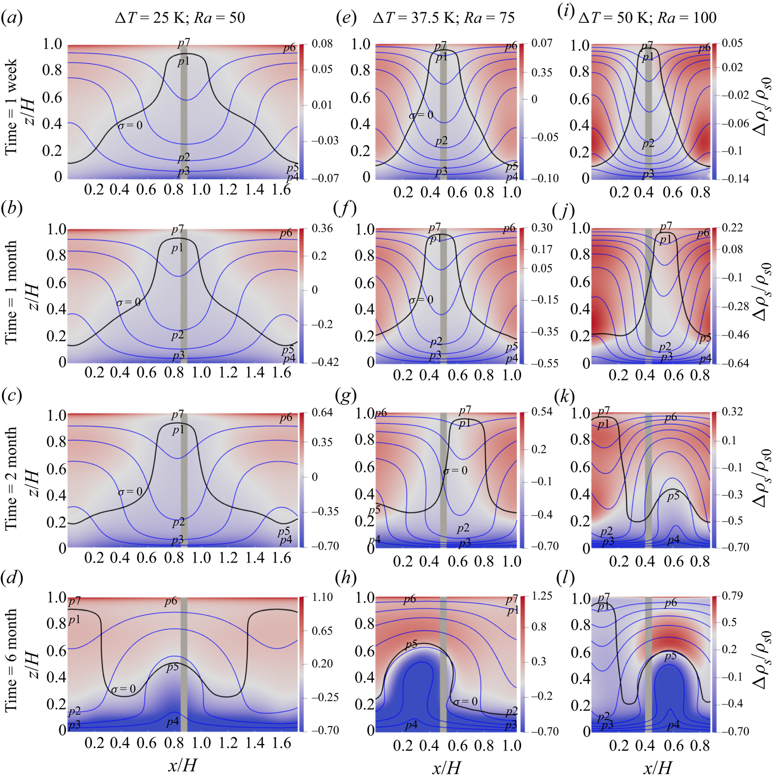
The time series of snow density change and the standard deviation of snow density change are shown in figure 14 for a general comparison of convective water vapour transport between three temperature differences. To reach for the first time the minimum snow density at the bottom, it takes 16.5, 8.5 and 6 weeks for the low-, medium- and high- $Ra$ cases, respectively. After six months of the simulation, the non-dimensional thickness for the low-density ‘weak layer’ with MPD for all cases is around
  $0.1H$. However, above this weak layer, there is another low-density layer until the non-dimensional height level of 0.2, 0.3 and 0.4 for the low-, medium- and high-
 $Ra$ cases respectively, in which the density decreases almost linearly due to phase change from 15 % (at top of the second weak layer) to 70 % (at top of the first weak layer). The medium- and high-
 $Ra$ cases have almost the same pattern for an increase in density on top with maximum values of 42.8 % (65.4 kg m
 $^{-3}$) and 47.4 % (72.3 kg m
 $^{-3}$) respectively. However, the low-
 $Ra$ case has two peaks for the density increase of which the first one is only 23.8 % (36.38 kg m
 $^{-3}$) while the second peak is very close to the top boundary with the significant value of 44 % (67.4 kg m
 $^{-3}$).
The time-series of (a–c) snow density change  $\Delta \rho _{s}$ and (d–f) the standard deviation of snow density change
  $\rho _{s,std}$ for three temperature differences.
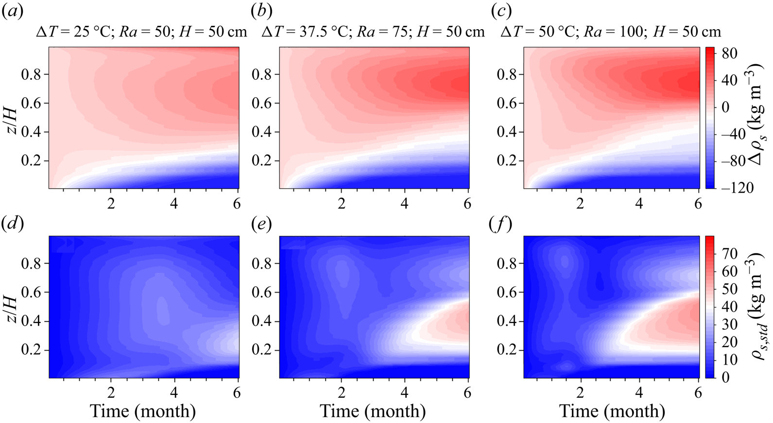
5.5. Scaling and order-of-magnitude analyses
5.5.1. Scaling argument
Non-dimensional governing equations and relevant scaling factors are introduced in detail in Appendix F. As shown in normalized equations, the controlling parameters for heat and mass transfer are  $Ra$ and
  $M=(6 \epsilon _{i} Sh_{ref})/(d_{p}^{*}\mkern -1.2mu^2 Ra Le_{m})$. A complete scaling is achieved when the influence of initial and boundary condition disappears (Barenblatt Reference Barenblatt1996). This would be the case for a system with only heat transfer (and no phase change) since the thermal boundary conditions are mapped from
  $[T_{c},T_{h}]$ to
  $[-1,0]$. In this case, the bottom/top thermal boundary layer thickness is only scaled and dependent on Rayleigh number (the non-dimensional temperature and temperature gradient are completely scalable and dependent on
  $Ra$). However, for the case with phase change, the scaling for water vapour distribution is not complete and it depends on both
  $Ra$ and bulk temperature difference. Using the Clausius–Clapeyron law for
  $\rho _{vs}= \rho _{vs_{ref}} \exp \left [ A (1/T_{ref}-1/T) \right ]$, where
  $A=L_{iv} m/(\rho _{i} k)$,
  $m$ is the mass of a water molecule and
  $k$ is the Boltzmann constant, we show the dependency of
  $\rho _{vs}^{*}\mkern -1.2mu$ and
  $\boldsymbol {\nabla }^{*}\mkern -1.2mu \rho _{vs}^{*}\mkern -1.2mu$ on
  $\Delta T$ and the reference temperature
  $T_{ref}$ as
 \begin{gather} \rho_{vs}^{*}\mkern-1.2mu = \frac{\rho_{vs}}{\rho_{vs_{ref}}} =\exp \left[ A \Delta T \frac{T^{*}\mkern-1.2mu }{T_{ref}(T^{*}\mkern-1.2mu+T_{ref}/\Delta T)} \right], \end{gather}
 \begin{gather} \boldsymbol{\nabla}^{*}\mkern-1.2mu \rho_{vs}^{*}\mkern-1.2mu =\frac{\boldsymbol{\nabla} \rho_{vs}}{\rho_{vs_{ref}}/H} =\frac{ {\rm d}\rho_{vs}/{\rm d}T\ \boldsymbol{\nabla} T}{\rho_{vs_{ref}}/H} ={\rho_{vs}}^{*}\mkern-1.2mu \boldsymbol{\nabla}^{*}\mkern-1.2mu T^{*}\mkern-1.2mu \frac{ A \Delta T}{(T^{*}\mkern-1.2mu+T_{ref}/\Delta T)^2}. \end{gather}
 Equations (5.1) suggest that phase change behaviour (which is directly connected to the water vapour density gradient as discussed earlier) cannot be completely scaled only by  $Ra$ and
  $M$. This may be shown by comparing two most similar cases for which both
  $Ra$ and
  $M$ are the same but the bulk temperature difference is different. As shown in figure 15, the non-dimensional porosity change rate and saturation degree are very different. For other cases in which the Rayleigh numbers are the same but with different
  $M$, the deviation and difference between cases are even larger, e.g. comparing figure 16 with figure 18 for non-dimensional temperature, temperature gradient, diffusive flux and flow velocity. Between the cases with same Rayleigh number, the smaller deviation in non-dimensional temperature (figure 17c,h) and temperature gradients (figure 17d,i) compared to deviation in diffusive water vapour density gradient (figure 17b,g) is directly linked to the relative contribution of phase change terms in energy and mass conservation equations, which is discussed in the next section. Overall, it appears that
  $Ra$ is effective in partially but not completely collapsing the non-dimensional profiles.
Non-dimensional results for two cases with the same  $Ra=50$ and
  $M=0.3514$ but different bulk temperature difference
  $\Delta T=25$ and
  $50$ K for (a,f) saturation degree
  $\sigma$, (b,g) rate of change for ice volumetric content
  ${\rm d}\epsilon _{i}/{\rm d}t^{*}\mkern -1.2mu$, (c,h) snow temperature
  $T_{m}^{*}\mkern -1.2mu$, (d,i) snow temperature gradient
  ${\rm d}T_{m}^{*}\mkern -1.2mu/{\rm d}z^{*}\mkern -1.2mu$ and (e,j) gas flow velocity
  $U_{g}^{*}\mkern -1.2mu$.

The relative error between two cases with the same  $Ra=50$ and
  $M=0.3514$ but different bulk temperature difference
  $\Delta T=25$ and
  $50$ K for the dimensionless results for (a,f) convective water vapour transport
  $\boldsymbol {\nabla } ^{*}\mkern -1.2mu \rho _{v}^{*}\mkern -1.2mu \boldsymbol {\cdot } U_{g}^{*}\mkern -1.2mu$, (b,g) diffusive water vapour flux
  $J_{v}^{*}\mkern -1.2mu$, (c,h) snow temperature
  $T_{m}^{*}\mkern -1.2mu$, (d,i) snow temperature gradient
  ${\rm d}T_{m}^{*}\mkern -1.2mu/{\rm d}z^{*}\mkern -1.2mu$ and (e,j) gas flow velocity
  $U_{g}^{*}\mkern -1.2mu$.

Non-dimensional results for (a,f) saturation degree  $\sigma$, (b,g) rate of change for ice volumetric content
  ${\rm d}\epsilon _{i}/{\rm d}t^{*}\mkern -1.2mu$, (c,h) snow temperature
  $T_{m}^{*}\mkern -1.2mu$, (d,i) snow temperature gradient
  ${\rm d}T_{m}^{*}\mkern -1.2mu/{\rm d}z^{*}\mkern -1.2mu$ and (e,j) gas flow velocity
  $U_{g}^{*}\mkern -1.2mu$. The cases with the same
  $Ra$ have the same colour in which the solid line is for larger
  $M$ and the dashed line is for smaller
  $M$.
$M$.
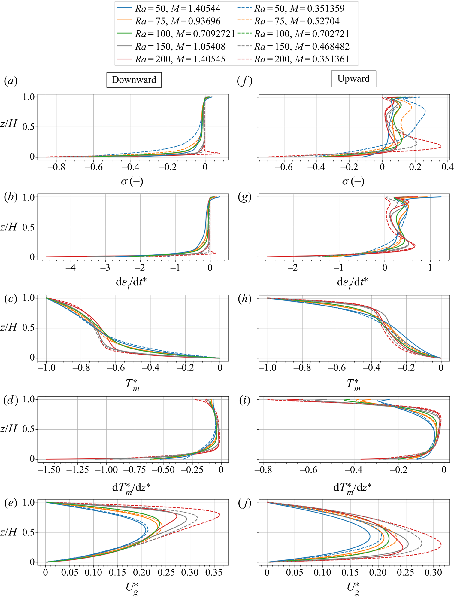
The relative error between two cases with the same  $Ra$ but different
  $M$ shown in figure 17 for the dimensionless results for (a,f) convective water vapour transport
  $\boldsymbol {\nabla } ^{*}\mkern -1.2mu \rho _{v}^{*}\mkern -1.2mu \boldsymbol {\cdot } U_{g}^{*}\mkern -1.2mu$, (b,g) diffusive water vapour flux
  $J_{v}^{*}\mkern -1.2mu$, (c,h) snow temperature
  $T_{m}^{*}\mkern -1.2mu$, (d,i) snow temperature gradient
  ${\rm d}T_{m}^{*}\mkern -1.2mu/{\rm d}z^{*}\mkern -1.2mu$ and (e,j) gas flow velocity
  $U_{g}^{*}\mkern -1.2mu$.

5.5.2. Analysis of dominant terms
The contributions of each term in gas and ice energy equations ((2.18) and (2.19) respectively) are shown in figures 19 and 20 for the horizontally averaged profiles and domain-averaged time series respectively. For the gas energy, the dominant term is convection but comparable with the conduction term. Figure 20 shows the relative magnitude as the ratio of each term (magnitude) to the summation of magnitude for all terms. The relative magnitudes of convection and conduction are 40 % and 35 % respectively (figure 20c). The heat transfer between phases is comparable to the net of convection and conduction terms while it is quite well matched with the ice conduction term (figure 20a,c). Its relative magnitudes in gas and ice energy equations are 20 % and 40 % respectively (figure 20c). This shows that we cannot neglect this term and this is the reason why the thermal equilibrium assumption is not valid. This is further shown in figure 21 for the temperature difference between gas and ice phases, in which the difference ranges from  $-5$ to 2 K. The phase change term in ice energy is much larger than that in gas energy with relative magnitudes of 15 % and 1 % respectively (figure 20c). However, the phase change term in ice energy is pronounced during the first month and later on it decreases gradually. Where the snow porosity increases laterally (at the bottom of the snowpack) and vertically (in MPD patches at bottom), the flow velocity grows and consequently both convection and conduction terms grow (figure 19a,b). Later on, at the middle of the snowpack, we observe that the convection term adds energy to the gas phase (figure 19a). This is because convection brings more energy through the MPD patches than the one leaving the deposition zone. This results in a convective energy flux convergence. We see that for the same area in the heat transfer term shown in figure 19(c), the energy is negative. This means the convective energy is converted to the heat transfer between two phases. The term associated with the gas pressure change (figure 19g), energy transport by diffusive flux (figure 19h) and temporal term (figure 19d) are negligible and much smaller than the other terms.


The relative magnitude and contribution of each term in (2.2) for the mass conservation of the water vapour component are shown in figures 20 and 22. During the first week of simulation when the convection cells are forming (stage 1 to stage 3 of thermal behaviour explained in § 5.1), the diffusion term is dominant at the bottom, while later the convection is dominant at the bottom and top of the snowpack (comparing figure 22e with figure 22f and also see figure 20d). At the bottom, once the porosity reaches the maximum possible value, the phase change stops and consequently both diffusion and convection balance each other. Also, on top, due to an increase in snow density, the convection contribution decreases gradually with time (figures 22e, 20b and 20d). As shown in figure 20(b,d), the dominant term in the mass conservation of the water vapour component is the phase change term with a relative magnitude of 45 % early in the simulation, which decreases gradually with time. The larger relative magnitude of the phase change term in the mass conservation equation of around 45 % compared with its contribution in the energy equation (approximately 15 %) supports that non-dimensional temperature and temperature gradient are partially scaling with  $Ra$ (within around 20 % deviation) while this is not the case at all for the phase change rate. Finally, similar to the energy equation, the temporal term for mass conservation of the water vapour component (figure 22d) is negligible and smaller than the other terms by two orders of magnitude.
The gas density gradient term (last term in (2.8)) is always upward in vertical flows (upward and downward) and it has the same direction as lateral flow on top. However, the dynamic pressure gradient is always downward in vertical flows and it has an opposite direction to the lateral flows on top. Hence, for the upward flow and also lateral flows on top, the gas density gradient term is the driving force and the dynamic pressure gradient and viscous forces are the opposite forces. However, for downward flow and also lateral flow at the bottom, the dynamic pressure gradient is larger and acts as driving force. As shown in figure 22(a), the buoyancy term is larger on top mainly because of  $|g z |$. Also, because of the no-flux condition, the dynamic pressure gradient must be the same as the gas density gradient term on top and bottom boundaries and its magnitude is larger on top, similar to the gas density gradient term. The viscous resistance force is two orders of magnitude smaller than the other terms in the momentum equation. Moreover, we see that the viscous resistance force gradually increases on top while decreasing at the bottom. The increase (decrease) in snow density results in decrease (increase) in both intrinsic permeability and flow velocity which has opposite effects in changing the viscous resistance force. However, the change in the intrinsic permeability is more pronounced than the change in flow velocity and it is the reason for increasing the resistance force on top (deposition zone) and decreasing it at the bottom (sublimation zone). Note that since the pore Reynolds number is much smaller than 1, the second term in the momentum equation is neglected and not presented in our analysis.
The horizontally averaged time series for the temperature difference between gas and ice phases.


6. Conclusions
In this paper, the effects of convective vapour transport for different snowpack conditions such as vertical size, thermal boundary conditions and Rayleigh number have been investigated numerically. To that end, a direct numerical solver based on the volume-averaged two-phase model has been implemented in the open-source fluid dynamics software OpenFOAM 5.0 (www.openfoam.org).
Investigating the scaling behaviour of our system, it is found that we do not have a complete scaling since heat and mass transfer are coupled by phase changes. It is discussed that we only have partially scaled results for interior temperature and its gradient but not for water vapour density and its gradient. We supported our argument by comparing the relative contribution of phase change terms in heat and mass transfer equations. Overall, it appears that  $Ra$ is effective in partially but not completely collapsing the non-dimensional profiles.
Analysing thermal and phase change regimes in detail, it is found that (1) the thermal and phase change behaviours in the upward and downward flows of a convection cell are qualitatively the same for snowpacks with different conditions, (2) once convection cells are completely formed, compared with the pure conduction temperature profile, the region is colder in downward flow and warmer in upward flow, (3) phase change rate is very small for the cold region on top in downward flow and a very small value for oversaturation  $\sigma$ of just around 0.05 is observed while for the warm region at the bottom, the sublimation rate is much larger, (4) the top region in downward flow has the lowest water vapour content while the bottom region in upward flow has the highest water vapour content, (5) there is a vertical effective deposition zone with a smaller saturation degree of less than around 0.2 while the effective sublimation zone is horizontal in the bottom region with saturation degree ranging from
  $-0.05$ to
  $-0.9$ and (6) convection cells are not fixed and may have horizontal displacements due to horizontal heterogeneity induced in the snow porosity. This leads to an almost uniform higher snow density close to the surface and a layer of significantly lower density at the bottom for the assumed temperature gradient of warmer temperatures at the bottom, which is the usual case in seasonal snow and on sea ice.
A significant influence of the snowpack size on the heat and mass transfer is observed: (1) for the sublimation zone in the downward flow, the larger the snowpack, the smaller the area in which the saturation degree magnitude is greater than 5 %, meaning that it has a smaller significant sublimation area in percentage compared to the smaller snowpacks, (2) at the bottom of snowpack in the upward flow, the larger snowpack reaches the saturation line closer to the bottom boundary, resulting in a smaller sublimation zone, (3) for the deposition region in the upward flow, while the small snowpack has more uniform and linear saturation degree and phase change rate, the large snowpack has two peaks in the saturation degree with a large saturation area in between and (4) the induced heterogeneity in snow porosity occurs faster and earlier and is stronger for the small snowpack due to its larger relative size (or extent) for the sublimation and deposition zones. During the first month of the simulation, the convection cell displacement is around  $0.8H$ for the small snowpack while it is only
  $0.15H$ for the medium snowpack.
Based on lateral averages for each level of  $z$, it is observed for small, medium and large snowpacks respectively that: (1) the weak layer at the bottom with the MPD has a non-dimensional thickness of around
  $0.2H$,
  $0.1H$ and
  $0.05H$, (2) it takes 5, 7 and 11 weeks to reach for the first time the minimum snow density at the bottom, (3) after six month of the simulation, the portion of the top region with density increase more than 25 % is around 46 %, 30 % and 10 %, (4) the maximum increase in density on top is 57 % (87 kg m
 $^{-3}$), 47 % (72 kg m
 $^{-3}$) and 29 % (45 kg m
 $^{-3}$) and (5) the MPD patches formed in the weak layer are larger for the small snowpack with vertical size of around
  $0.5H$. As a result, the standard deviation for the snow density change is larger for the small snowpack around 70 kg m
 $^{-3}$ while it is around 50 and 40 kg m
 $^{-3}$ for the medium and large ones.
Results of various temperature differences indicate that (1) in both downward and upward flows far from the bottom boundary, the high- $Ra$ case even with a smaller saturation vapour density gradient has a larger snow density change as its convective flow velocity is higher; however, it has almost the same snow density change compared with the medium-
 $Ra$ case in the upper half of the domain while a larger snow density change in the lower half, (2) in both downward and upward flows close to the bottom boundary, snow density change is larger for the case of higher
  $Ra$ because of its stronger saturation density gradient, (3) it takes 16.5, 8.5 and 6 weeks for the low-, medium- and high-
 $Ra$ cases respectively to reach the minimum snow density at the bottom and (4) the maximum increase in density on top for medium- and high-
 $Ra$ cases is around 42.8 % (65.4 kg m
 $^{-3}$) and 47.4 % (72.3 kg m
 $^{-3}$) respectively. The low-
 $Ra$ case has two peaks for the density increase with a maximum one very close to the top boundary of 44 % (67.4 kg m
 $^{-3}$).
The model system simulated and analysed in this study is a considerably simplified representation of a naturally occurring snowpack. A very important process, not considered here, is the densification of snow due to metamorphism and overburden pressure arising from its own weight. Additionally the effect of wind pumping and the exchange of vapour with the atmosphere is also neglected. This effect was tested in sensitivity simulations to verify and confirm that its effect is small (see figure 30 in Appendix E). In spite of these simplifications, there are indeed vast areas of naturally occurring snowpacks, such as those in the polar regions or on sea ice, for which convection should be very important and likely needs to be considered ( Appendix G). This study was motivated by the long-standing debate in the cryospheric community about the relevance of vapour convection in snowpacks. There have been various field campaigns and reports that invoke vapour convection as the only plausible mechanism to explain observations of temperature and density distributions. This study was the first attempt to use a fluid-dynamics-based, numerical approach to investigate convection in snow. Our current and future work is to expand our numerical modelling to simulate more realistic scenarios where there is multi-scale heterogeneity, i.e realistic layering and lateral variations. The model system in this study, with its homogeneous boundary conditions and simple bottom geometry is in fact the most restrictive in triggering and sustaining convection. This study thus establishes the ‘baseline’ for future explorations. For example, there is long-standing evidence by Sturm & Johnson (Reference Sturm and Johnson1991) who reported implications of convective transport in natural snowpacks with  $Ra$ as low as 5. It is highly likely that their and many other natural systems are heavily influenced by heterogeneity.
We demonstrated that the new model reproduces a low-density layer and a high-density layer respectively at the bottom and top of snow covers and, especially for thin snow covers, the high-density layer on top is often observed together with density decreases at the bottom. This has not been possible to reproduce with current snow models. While settling will partially counteract the generation of this low-density layer at the bottom, we note that the generation of asymmetric depth hoar crystals as a result of vapour transport allows for quite low-density patches between chains of supporting depth hoar structures. The high porosity between such chains will help to keep convection going in real snow covers. For future work, the model developed in this paper for convective vapour transport will therefore be used to improve the one-dimensional physics-based multi-layer snow model by a tight coupling between OpenFOAM and SNOWPACK (Lehning et al. Reference Lehning, Bartelt, Brown, Russi, Stöckli and Zimmerli1999), in which lateral averages of the porosity change due to convective vapour transport will be fed into SNOWPACK.
Funding
This project is co-supported by the Swiss National Science Foundation-SNF, grant number 200021E-154248, and the Deutsche Forschungsgemeinschaft (DFG) in the framework of the priority programme ‘Antarctic research with comparative investigations in Arctic ice areas’ under grant numbers NI 1096/5-1 and KA 2694/7-1. Further support by the Swiss National Supercomputing Facility CSCS (grant number S938) is acknowledged.
Declaration of interests
The authors report no conflict of interest.
Code availability
The source code for  $\textit {snowpackBuoyantPimpleFoam}$ developed and used in this paper is available in the EnviDat repository (Jafari & Lehning Reference Jafari and Lehning2021).
Appendix A. Results of the sensitivity analysis for the initial values
The sensitivity analysis for the initial temperature and vapour distribution is shown in figure 23.
Comparison of the results for two different initial values. (a) Dry snowpack  $\sigma =-1$ compared with the saturation vapour density
  $\sigma =0$. (b) The initial temperatures of
  $T_c$ and
  $T_h$ are compared.

Appendix B. Results of the sensitivity analysis for the maximum Courant number
The sensitivity analyses for the maximum Courant number after 1 month and 6 months of simulation are shown in figures 24 and 25 respectively.
Comparison of the results for different maximum Courant numbers after a month of simulation. (a) The snow density change, (b) the snow temperature and (c) the gas flow velocity.

Appendix C. Results of the sensitivity analysis for the domain width
The sensitivity analysis of the domain width for the normalized snow density is shown in figure 26. Also, comparisons of the normalized convection cell size for different domain width for the case without and with phase change are shown in figures 27 and 28 respectively.
Comparison of the results for different maximum Courant numbers after 6 months of simulation. (a) The snow density change, (b) the snow temperature and (c) the gas flow velocity.

Comparison of the normalized snow density for different domain lengths with  $Ra=100$,
  $H=50$ cm and
  $\Delta T=50\,{\rm K}$.

Comparison of the normalized convection cell size for different domain widths for the case without phase change.

Appendix D. Qualitative analysis of the phase change rate
To analyse the local mass transfer regime, we rely on the qualitative dependency of the phase change rate (or saturation degree) on both the convective flow rate and the gradient of the saturation vapour density. Extending the convection term of the steady-state continuity equations for the air component and gas mixture and also neglecting the diffusion term due to its small relative contribution compared with convection, we have the following equations respectively:
 \begin{gather} \left\langle \rho_{g} \right\rangle^{g} \boldsymbol{\nabla}\boldsymbol{\cdot} \left\langle \boldsymbol{U}_{g} \right\rangle + \left\langle \boldsymbol{U}_{g} \right\rangle \boldsymbol{\cdot} \boldsymbol{\nabla} \left\langle \rho_{g} \right\rangle^{g} = \dot{m_{iv}}, \end{gather}
 \begin{gather} \left\langle \rho_{a} \right\rangle^{g} \boldsymbol{\nabla}\boldsymbol{\cdot} \left\langle \boldsymbol{U}_{g} \right\rangle ={-}\left\langle \boldsymbol{U}_{g} \right\rangle \boldsymbol{\cdot} \boldsymbol{\nabla}\left\langle \rho_{a} \right\rangle^{g}. \end{gather}
 Using the approximation  $\left \langle \rho _{g} \right \rangle ^{g} \approx \left \langle \rho _{a} \right \rangle ^{g}$ in the first term of (D1) and then replacing it with the term on the right-hand side of (D2) and simplifying, we have finally the driving force for the mass transfer as
 \begin{equation} \left\langle \boldsymbol{U}_{g} \right\rangle \boldsymbol{\cdot} \boldsymbol{\nabla}\left\langle \rho_{v} \right\rangle^{g} = \dot{m_{iv}}. \end{equation}
Note that in (D3), for the qualitative analysis, the water vapour density gradient may be approximated by the gradient of saturation vapour density. As shown in figure 29, this is because  $\rho _{v}=(1+\sigma )\rho _{vs}$ means that the vapour density is directly correlated to saturation vapour density.
Comparison of the normalized convection cell size for different domain widths for the case with phase change.

One-dimensional profiles of the saturation vapour density  $\rho _{vs}$ and vapour density
  $\rho _{v}$ at the location of downward and upward flows of a convection cell for different snow heights
  $H$, and the temperature difference
  $\Delta T$, all after a week of simulation.

Appendix E. A test case for the wind pumping effect
We performed a test case for different snow heights to investigate the wind pumping effect when natural convection is active in the system. To this end, the perturbation by wind turbulence is randomly sampled by the normal Gaussian distribution as wind-turbulent ventilation is a high-frequency phenomenon. In the sampling distribution with a standard deviation of 1, the mean ventilation velocity is considered as  $0.05$ cm s
 $^{-1}$ which is reported by Colbeck (Reference Colbeck1989) and Waddington et al. (Reference Waddington, Cunningham and Harder1996). Since for each cell face on the top boundary the ventilation velocity is sampled randomly, we modified the resulting sampled velocities to guarantee that the net air flux on the top boundary is zero due to air mass conservation in the whole system. Note that in spite of zero net gas (air and vapour) flux, there is still a non-zero vapour flux, both locally and globally, and thus the system is ‘open’ for water vapour. Comparing the cases with and without ventilation, we found almost no difference in laterally averaged snow density change profile as shown in figure 30. Note that this was expected since the ventilation velocity of
  $0.05$ cm s
 $^{-1}$ is almost one order of magnitude smaller than the convective velocity scale
  $U_{conv}$. Obviously, larger ventilation velocities might lead to a stronger disturbance in convection cells and if strong enough it may stop and shut down the convection in the snowpack. Moreover, in many Arctic snow covers and for snow on sea ice, a hard crust or wind slab frequently develops at the surface. With such a hard surface, our assumption is less unrealistic.
Comparison of the results for a case without wind pumping and a case with a ventilation velocity of 0.05 cm s $^{-1}$: (a)
  $Ra = 50$,
  $H = 25$ cm; (b)
  $Ra = 100$,
  $H = 50$ cm; (c)
  $Ra = 200$,
  $H = 100$ cm.

Appendix F. Non-dimensional governing equations
The scaling factors for the length, pressure and density gradient are selected as  $H$,
$H$,  $\rho \beta \Delta T g H$ and
  $\rho \beta \Delta T/H$ respectively. Note that
  $\rho _{a0}$ is used for the gas mixture density whereas
  $\rho _{vs_0}$ (saturation vapour density at
  $T_{ref}$) is used for the water vapour density as scaling factor. The effective thermal conductivities and the intrinsic permeability all both scaled based on the initial porosity as
  $k_{{eff},s0}$ and
  $K_{0}$ respectively. Since convection is the dominant transport mechanism, the reference velocity and time scales are chosen as
  $U_{conv}$ and
  $H/U_{conv}$ respectively. The dimensionless variables with superscript asterisk are as follows:
 \begin{gather} t^{*}=\frac{t}{H/U_{conv}};\quad x^{*}=\frac{x}{H};\quad z^{*}=\frac{z}{H};\quad \boldsymbol{\nabla}^{*}\mkern-1.2mu=\frac{\boldsymbol{\nabla}}{H}, \end{gather}
 \begin{gather} \left\langle T_{g}^{*}\mkern-1.2mu \right\rangle^{g}=\frac{\left\langle T_{g} \right\rangle^{g}-T_{h}}{T_{h}-T_{c}};\quad \left\langle T_{i}^{*}\mkern-1.2mu \right\rangle^{i}=\frac{\left\langle T_{i} \right\rangle^{i}-T_{h}}{T_{h}-T_{c}}, \end{gather}
 \begin{gather} \left\langle \rho_{g}^{*}\mkern-1.2mu \right\rangle^{g}=\frac{\left\langle \rho_{g} \right\rangle^{g}}{\rho_{a_{ref}}};\quad \left\langle \rho_{v}^{*}\mkern-1.2mu \right\rangle^{g}=\frac{\left\langle \rho_{v} \right\rangle^{g}}{\rho_{vs_{ref}}};\quad \left\langle \rho_{a}^{*}\mkern-1.2mu \right\rangle^{g}=\frac{\left\langle \rho_{a} \right\rangle^{g}}{\rho_{a_{ref}}};\quad \left\langle J_{v}^{*}\mkern-1.2mu \right\rangle=\frac{\left\langle J_{v} \right\rangle}{D_{va} \rho_{vs_{ref}}/H}, \end{gather}
 \begin{gather} \left\langle U_{g}^{*}\mkern-1.2mu \right\rangle=\frac{\left\langle U_{g} \right\rangle}{U_{conv}};\quad \left\langle P_{g}^{*}\mkern-1.2mu \right\rangle^{g}=\frac{\left\langle P_{g} \right\rangle^{g}}{\rho_{a_{ref}} \beta \Delta T g H};\quad \boldsymbol{\nabla}^{*}\mkern-1.2mu\left\langle \rho_{g}^{*}\mkern-1.2mu \right\rangle^{g}=\frac{\boldsymbol{\nabla}\left\langle \rho_{g} \right\rangle^{g}}{\rho_{a_{ref}} \beta \Delta T/H}, \end{gather}
 \begin{gather} D_{{eff},s}^{*}\mkern-1.2mu=\frac{D_{{eff},s}}{D_{va}};\quad k_{{eff},g}^{*}\mkern-1.2mu=\frac{k_{{eff},g}}{k_{{eff},s0}};\quad k_{{eff},i}^{*}\mkern-1.2mu=\frac{k_{{eff},i}}{k_{{eff},s0}};\quad c_{pg}^{*}\mkern-1.2mu=\frac{c_{pg}}{c_{pa}};\quad d_{p}^{*}\mkern-1.2mu=\frac{d_{p}}{H}. \end{gather}
Using the defined scaling factors and dimensionless variables, the final set of (2.1), (2.2) and (2.3) for the mass conservation, (2.8) for the momentum and (2.18) and (2.19) for the temperature-based energy equations are normalized respectively as follows to extract the group of non-dimensional numbers important for the convection of water vapour in the snowpack:
 \begin{equation} \frac{\partial}{\partial t^{*}\mkern-1.2mu} \left(\epsilon_{g} \left\langle \rho_{g}^{*}\mkern-1.2mu \right\rangle^{g}\right)+ \boldsymbol{\nabla}^{*}\boldsymbol{\cdot} \left( \left\langle \rho_{g}^{*}\mkern-1.2mu \right\rangle^{g} \left\langle \boldsymbol{U}_{g}^{*}\mkern-1.2mu \right\rangle\right) ={-}\left[ \frac{\rho_{vs_{ref}}}{\rho_{a_{ref}}} \frac{6 \epsilon_{i} Sh_{ref}}{ d_{p}^{*}\mkern-1.2mu^2 Ra Le_{m}} \right] \sigma, \end{equation}
 \begin{equation} \frac{\partial}{\partial t^{*}\mkern-1.2mu}\left(\epsilon_{g} \left\langle \rho_{v}^{*}\mkern-1.2mu \right\rangle^{g}\right)+ \boldsymbol{\nabla}^{*}\boldsymbol{\cdot} \left( \left\langle \rho_{v}^{*}\mkern-1.2mu \right\rangle^{g} \left\langle \boldsymbol{U}_{g}^{*}\mkern-1.2mu \right\rangle\right) = \left[ \frac{1}{Ra Le_{m}} \right] \boldsymbol{\nabla}^{*}\boldsymbol{\cdot} \left(D_{{eff},s}^{*}\mkern-1.2mu \boldsymbol{\nabla}^{*}\mkern-1.2mu \left\langle \rho_{v}^{*}\mkern-1.2mu \right\rangle^{g}\right) -\left[ \frac{6 \epsilon_{i} Sh_{ref}}{ d_{p}^{*}\mkern-1.2mu^2 Ra Le_{m}} \right] \sigma, \end{equation}
 \begin{equation} \frac{\partial \epsilon_{i}}{\partial t^{*}\mkern-1.2mu} = \left[ \frac{\rho_{vs_{ref}}}{\rho_{i}} \frac{6 \epsilon_{i} Sh_{ref}}{ d_{p}^{*}\mkern-1.2mu^2 Ra Le_{m}} \right] \sigma, \end{equation}
 \begin{equation} -\frac{\left\langle \boldsymbol{U}_{g}^{*}\mkern-1.2mu \right\rangle}{K^{*}\mkern-1.2mu} -\frac{ \left\langle \rho_{g}^{*}\mkern-1.2mu \right\rangle^{g} c_{F} }{\sqrt{K^{*}\mkern-1.2mu}} \left| \left\langle \boldsymbol{U}_{g}^{*}\mkern-1.2mu \right\rangle \right| \left\langle \boldsymbol{U}_{g}^{*}\mkern-1.2mu \right\rangle \left[ \frac{Ra \sqrt{Da}}{ Pr_{m}} \right] - \boldsymbol{\nabla}^{*}\mkern-1.2mu\left\langle P_{g}^{*}\mkern-1.2mu \right\rangle^{g} + \boldsymbol{\nabla}^{*}\mkern-1.2mu\left\langle \rho_{g}^{*}\mkern-1.2mu \right\rangle^{g} z^{*}\mkern-1.2mu = 0, \end{equation}
 \begin{align} &\frac{\partial}{\partial t^{*}\mkern-1.2mu}\left(\epsilon_{g} \left\langle \rho_{g}^{*}\mkern-1.2mu \right\rangle^{g} c_{pg}^{*}\mkern-1.2mu \left\langle T_{g}^{*}\mkern-1.2mu \right\rangle^{g}\right) + \boldsymbol{\nabla}^{*}\boldsymbol{\cdot} \left( \left\langle \rho_{g}^{*}\mkern-1.2mu \right\rangle^{g} c_{pg}^{*}\mkern-1.2mu \left\langle T_{g}^{*}\mkern-1.2mu \right\rangle^{g} \left\langle \boldsymbol{U}_{g}^{*}\mkern-1.2mu \right\rangle\right)\nonumber\\ &\quad = \left[ \frac{1}{Ra} \right] \boldsymbol{\nabla}^{*}\boldsymbol{\cdot} \left(\epsilon_{g} k_{{eff},g}^{*}\mkern-1.2mu \boldsymbol{\nabla}^{*}\mkern-1.2mu\left\langle T_{g}^{*}\mkern-1.2mu \right\rangle^{g}\right) \nonumber\\ &\qquad+\left[ Ge \right] \left( \epsilon_{g} \frac{\partial}{\partial t^{*}\mkern-1.2mu} \left\langle P_{g}^{*}\mkern-1.2mu \right\rangle^{g} +\left\langle \boldsymbol{U}_{g}^{*}\mkern-1.2mu \right\rangle \boldsymbol{\cdot} \boldsymbol{\nabla}^{*}\mkern-1.2mu\left\langle P_{g}^{*}\mkern-1.2mu \right\rangle^{g} \right)\nonumber\\ &\qquad-\left[ \frac{ \rho_{vs_{ref}} (c_{pv}-c_{pa})}{\rho_{a_{ref}} c_{pa}} \frac{1}{Ra Le_{m}} \right] \boldsymbol{\nabla}^{*}\boldsymbol{\cdot} \left(\left\langle T_{g}^{*}\mkern-1.2mu \right\rangle^{g} \left\langle J_{v}^{*}\mkern-1.2mu \right\rangle\right)\nonumber\\ &\qquad+\left[ \frac{6 \epsilon_{i} Sh_{ref} Le_{ref}}{ d_{p}^{*}\mkern-1.2mu^2 \rho_{vs}^{*}\mkern-1.2mu Ra Le_{m}} \right] \left(\left\langle T_{g}^{*}\mkern-1.2mu \right\rangle^{g} (w_{g}-1)+\left\langle T_{i}^{*}\mkern-1.2mu \right\rangle^{i} w_{i}\right)\nonumber\\ &\qquad-\left[ \frac{\rho_{vs_{ref}} c_{pv}}{\rho_{a_{ref}} c_{pa}} \frac{6 \epsilon_{i} Sh_{ref}}{ d_{p}^{*}\mkern-1.2mu^2 Ra Le_{m}} \right] \sigma \left\langle T_{g}^{*}\mkern-1.2mu \right\rangle^{g}, \end{align}
 \begin{align} \frac{\partial}{\partial t^{*}\mkern-1.2mu}\left(\epsilon_{i} \left\langle T_{i}^{*}\mkern-1.2mu \right\rangle^{i}\right) &= \left[ \frac{\rho_{a_{ref}} c_{pa}}{\rho_{i} c_{pi}} \frac{1}{Ra} \right] \boldsymbol{\nabla}^{*}\boldsymbol{\cdot} \left(\epsilon_{i} k_{{eff},i}^{*}\mkern-1.2mu \boldsymbol{\nabla}^{*}\mkern-1.2mu\left\langle T_{i}^{*}\mkern-1.2mu \right\rangle^{i}\right)\nonumber\\ &\quad -\left[ \frac{\rho_{a_{ref}} c_{pa}}{\rho_{i} c_{pi}} \frac{6 \epsilon_{i} Sh_{ref} Le_{ref}}{ d_{p}^{*}\mkern-1.2mu^2 \rho_{vs}^{*}\mkern-1.2mu Ra Le_{m}} \right] \left(\left\langle T_{g}^{*}\mkern-1.2mu \right\rangle^{g} (w_{g}-1)+\left\langle T_{i}^{*}\mkern-1.2mu \right\rangle^{i} w_{i}\right)\nonumber\\ &\quad +\left[ \frac{\rho_{vs_{ref}} c_{pv}}{\rho_{i} c_{pi}} \frac{6 \epsilon_{i} Sh_{ref}}{ d_{p}^{*}\mkern-1.2mu^2 Ra Le_{m}} \right] \sigma \left(\left\langle T_{g}^{*}\mkern-1.2mu \right\rangle^{g} w_{g}+\left\langle T_{i}^{*}\mkern-1.2mu \right\rangle^{i} w_{i}\right)\nonumber\\ &\quad +\left[ \frac{\rho_{vs_{ref}}(c_{pi}-c_{pv}) T_{ref}}{\rho_{i} c_{pi} \Delta T} \frac{6 \epsilon_{i} Sh_{ref}}{ d_{p}^{*}\mkern-1.2mu^2 Ra Le_{m}} \right] \sigma\nonumber\\ &\quad +\left[ \frac{\rho_{vs_{ref}}L_{iv}}{\rho_{i} c_{pi} \Delta T} \frac{6 \epsilon_{i} Sh_{ref}}{ d_{p}^{*}\mkern-1.2mu^2 Ra Le_{m}} \right] \sigma. \end{align}
In the above set of equations, groups of non-dimensional numbers are put inside the brackets. Also, for the sake of convenience, the group of non-dimensional numbers on the right-hand side of (F7) is named as  $M=(6 \epsilon _{i} Sh_{ref})/(d_{p}^{*}\mkern -1.2mu^2 Ra Le_{m})$, which appears in other terms. The other non-dimensional numbers in the above equations include the Sherwood number, the Lewis number, the reference Lewis number, the Prandtl number, the Darcy number and finally the Gebhart number, which are given as follows:
 \begin{gather} Sh_{ref}=\frac{ \rho_i d_{p} }{\mathcal{B} \rho_{vs_{ref}} D_{va}}, \end{gather}
 \begin{gather} Le_m=\frac{ k_{{eff},s0} }{ \rho_{a,{ref}}c_{pa} D_{va} };\quad Le_{ref}=\frac{ k_{a} }{ \rho_{a,{ref}}c_{pa} D_{va} }, \end{gather}
 \begin{gather} Pr_{m}=\frac{ k_{{eff},s0} }{ \rho_{a,{ref}}c_{pa} }, \end{gather}
 \begin{gather} Da=\frac{ K_{0} }{ H^{2} }, \end{gather}
 \begin{gather} Ge=\frac{ \beta g H }{ c_{pa} }. \end{gather}
As shown in these normalized equations, for both heat and mass transfer, the controlling parameters are  $Ra$,
$Ra$,  $Le_{m}$ and
  $d_{p}^{*}\mkern -1.2mu$ (as they appear in the parameter
  $M$), meaning that the mass transfer regime cannot be abstracted only by
  $Ra$. The term
  $M$ can be interpreted as the dimensionless mass transfer coefficient and
  $\sigma$ as the potential or driving force for the mass transfer. By expanding parameter
  $M$, one can show that for a specified porosity and grain size,
  $M$ is indeed a function of the inverse characteristic temperature gradient
  $\Delta T/H$.
Appendix G. Model system and real-world analogues
The conditions that we assume in our idealized set-up are realistic and can be found in snowpacks in the polar regions, and especially for snow on sea ice, where the temperature at the bottom remains always close to melting if the ice is thin and the surface can get very cold. But also in other snow covers, conditions can be found that are close to those of our idealized set-up. We discuss this now in more detail and provide the references as follows:
(i) Snow density. there are many areas in the cryosphere that are subjected to perhaps only a few snowfall events during the entire winter period. Examples include vast expanses of Siberia and the Arctic (Gouttevin et al. Reference Gouttevin, Langer, Löwe, Boike, Proksch and Schneebeli2018; Jafari et al. Reference Jafari, Gouttevin, Couttet, Wever, Michel, Sharma, Rossmann, Maass, Nicolaus and Lehning2020), or, for instance Tibet. In many of these areas, a singular snowfall event with new snow densities well below 100 kg m
$^{-3}$ can be found and low densities can persist for multiple months. In the polar regions in particular, absence of solar radiation and persistent low temperatures throughout the winter months help to limit settling in these conditions. Thus even the very idealized case in this study has many real-world analogues.(ii) Temperature gradients. Temperature gradients of
${O} ( 100 )$ K m$^{-1}$ are quite common in snowpacks. For example, our own previous work on vapour diffusion (Jafari et al. Reference Jafari, Gouttevin, Couttet, Wever, Michel, Sharma, Rossmann, Maass, Nicolaus and Lehning2020) discusses data from Samoylov, shown in figure 1(a) of Jafari et al. (Reference Jafari, Gouttevin, Couttet, Wever, Michel, Sharma, Rossmann, Maass, Nicolaus and Lehning2020). In Samoylov, we can see persistent negative temperature gradients of 100–200 K m$^{-1}$ over a period of 4–5 months interrupted only by the onset of spring (figure 1a of Jafari et al. Reference Jafari, Gouttevin, Couttet, Wever, Michel, Sharma, Rossmann, Maass, Nicolaus and Lehning2020).(iii) Bottom thermal boundary at
$0\,^\circ {\rm C}$. For snow on sea ice, where the temperature at the bottom remains always close to melting if the ice is thin and the surface can get very cold (Nicolaus & Schwegmann Reference Nicolaus and Schwegmann2017; Wever et al. Reference Wever, Rossmann, Maaß, Leonard, Kaleschke, Nicolaus and Lehning2020).


 Open access