2.1 Direct numerical simulation database

To be used for the development of closures, the DNS data employed have to provide resolved information about the respective processes. For the present work, this requires DNS with geometrically resolved bubbles. Extracting statistical information from such simulations about interfacial terms is by no means trivial (Santarelli et al. Reference Santarelli, Roussel and Fröhlich2016). Furthermore, to provide relevant data for modelling, the effect considered should be of sizeable, if not dominating, impact in the reference case selected. This second condition is also met with the flows considered here, which are governed by the balance between production of TKE through BIT and dissipation.

In Santarelli & Fröhlich (Reference Santarelli and Fröhlich2015, Reference Santarelli and Fröhlich2016) bubble-resolving DNS with many thousands of bubbles at low Eötvös number were conducted. Bubbles were considered as spherical objects of fixed shape and a no-slip condition was applied at the phase boundary, matching with the behaviour of air bubbles rising in contaminated water. Compared to other simulations of this type (Ilić Reference Ilić2006; Erdogan & Wörner Reference Erdogan and Wörner2014), these simulations are substantially closer to applications in that they involve turbulent background flow, contaminated fluid, realistic density ratio, higher bubble Reynolds number, a much larger domain and a much larger number of bubbles.

Figure 1.

Instantaneous DNS data for the case SmMany of Santarelli & Fröhlich (Reference Santarelli and Fröhlich2015). The bubble size is to scale and the vertical plane with the contour plot shows the instantaneous streamwise liquid velocity. (Main part of the picture reprinted from Santarelli (Reference Santarelli2015) with permission from TUDpress.)

Table 1.

Parameters of the cases used for the present study according to Santarelli & Fröhlich (Reference Santarelli and Fröhlich2015, Reference Santarelli and Fröhlich2016). The labels Sm and La used for the case with the bidisperse bubble swarm, BiDisp, indicate averaging over the small and large bubbles of the case BiDisp, respectively. Here, $N_{p}$ is the number of bubbles, $\unicode[STIX]{x1D6FC}$ the void fraction, $d_{p}$ the particle diameter and $Ar$ the Archimedes number. The values of $Re_{\unicode[STIX]{x1D70F}}$, the friction Reynolds number, $Re_{p}$, the particle Reynolds number based on $d_{p}$ and the relative velocity, and $C_{D}$, the drag coefficient obtained according to (4.4) below, are results of the simulations.

The DNS were conducted for upward vertical flow between two flat walls in a channel, with $x$ the streamwise, $y$ the wall-normal and $z$ the spanwise coordinate. The size of the computational domain is $L_{x}\times L_{y}\times L_{z}=4.41H\times H\times 2.21H$, where $H$ is the distance between the walls. Figure 1 shows the domain and an instantaneous snapshot of the bubbly flow in one of the DNS cases, labelled SmMany. A no-slip condition was applied at the walls and periodic conditions in $x$ and $z$. The gravitational force acts in the negative $x$-direction, and the bulk velocity $U_{b}$ was kept constant by instantaneously adjusting a volume force, equivalent to a pressure gradient, thus imposing a desired bulk Reynolds number $Re_{b}=U_{b}H/\unicode[STIX]{x1D708}$, where $\unicode[STIX]{x1D708}$ is the kinematic viscosity of the liquid. The DNS were all conducted with $Re_{b}=5263$. The data used in this work were obtained for three monodisperse cases (SmMany, SmFew, LaMany) and one bidisperse case labelled BiDisp, of the same void fraction as SmMany and LaMany with half the void fraction consisting of smaller bubbles and the other half of larger bubbles. Additionally, a single-phase simulation labelled Unladen was performed under the same conditions for comparison. Table 1 provides an overview of all cases with the corresponding labels. The data available cover statistical moments of first and second order for liquid and bubbles, as well as two-point correlations. The technically involved numerical procedure to evaluate the TKE budget was presented in Santarelli et al. (Reference Santarelli, Roussel and Fröhlich2016).

While the DNS were performed using a non-dimensional set of parameters, the EE SMC proposed in the present study is related to the size of bubble $d_{p}$, with the corresponding simulations performed in dimensional units. For this reason, the above set-up is converted to a dimensional form using the contaminated air–water system as an example. Based on the discussion in Ern et al. (Reference Ern, Risso, Fabre and Magnaudet2012), the pivoting element is chosen to be the equality of the Archimedes number, $Ar$, defined as

(2.1)$$\begin{eqnarray}Ar=\frac{|\unicode[STIX]{x1D70C}^{G}-\unicode[STIX]{x1D70C}^{L}|gd_{p}^{3}}{\unicode[STIX]{x1D70C}^{L}\unicode[STIX]{x1D708}^{2}},\end{eqnarray}$$

with $g$ the gravity. This leads to an accurate interpretation of the real effect of buoyancy in the considered DNS. Keeping $Ar$ the same as in the DNS and using all the other physical dimensional parameters on the right-hand side of (2.1) yields $d_{p}=1.456~\text{mm}$ for the smaller bubbles and $d_{p}=2.127~\text{mm}$ for the larger bubbles. The ratio $d_{p}/H$ in table 1 for the different cases then results in the extensions $123.6~\text{mm}\times 28.0~\text{mm}\times 61.8~\text{mm}$ of the channel.

2.2 Limitations of eddy-viscosity models for bubbly flow

Figure 2.

Distribution of $C_{\unicode[STIX]{x1D707}}$ in a $k$–$\unicode[STIX]{x1D700}$ type model computed using DNS data.

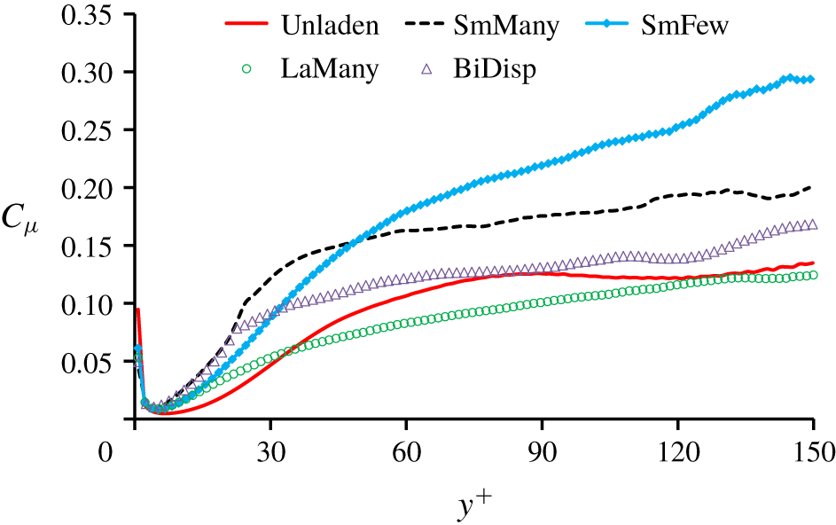
Figure 2 clarifies a special shortcoming of all EE $k$–$\unicode[STIX]{x1D700}$ type models for bubbly flows constituting one of several motivations to develop the present EE SMC. Figure 2 was constructed from the DNS data (table 1) and shows an evaluation of the constant $C_{\unicode[STIX]{x1D707}}$, which can be expressed using the definition of the turbulent viscosity (Jones & Launder Reference Jones and Launder1972)

(2.2)$$\begin{eqnarray}C_{\unicode[STIX]{x1D707}}=\frac{\unicode[STIX]{x1D708}_{t}\unicode[STIX]{x1D700}}{k^{2}}\end{eqnarray}$$

in terms of $k=\frac{1}{2}\overline{\overline{u_{i}^{\prime }u_{i}^{\prime }}}$ and $\unicode[STIX]{x1D700}=(1/\unicode[STIX]{x1D70C})\overline{\unicode[STIX]{x1D711}}\,\overline{\overline{\unicode[STIX]{x1D70F}_{ij}^{\prime }(\unicode[STIX]{x2202}u_{i}^{\prime }/\unicode[STIX]{x2202}x_{j})}}$, with $\unicode[STIX]{x1D70F}_{ij}^{\prime }$ the fluctuating viscous stress tensor (Kataoka & Serizawa Reference Kataoka and Serizawa1989; Kataoka et al. Reference Kataoka, Besnard and Serizawa1992). Here, $\overline{\overline{\cdots \,}}$ denotes the phase-weighted averaging, defined by $\overline{\overline{F}}=\overline{F\unicode[STIX]{x1D711}}/\overline{\unicode[STIX]{x1D711}}$, where $\overline{\cdots \,}$ represents the Reynolds (or statistical) averaging with respect to time, space or ensemble of realizations. In these expressions, $\unicode[STIX]{x1D711}$ is an indicator function for the liquid phase, defined by $\unicode[STIX]{x1D711}(\boldsymbol{x},t)=1$ if $(\boldsymbol{x},t)$ in the liquid phase and equal to zero otherwise. Fluctuations of liquid quantities are defined as $F^{\prime }=F-\overline{\overline{F}}$.

As shown in Santarelli et al. (Reference Santarelli, Roussel and Fröhlich2016), the BIT term dominates for $y^{+}\gtrsim 30$, being equilibrated by the dissipation term only. The mean liquid velocity profile $\overline{\overline{u}}$ becomes flat in the channel centre, so that $\unicode[STIX]{x2202}\overline{\overline{u}}/\unicode[STIX]{x2202}y$ approaches zero and $\unicode[STIX]{x1D708}_{t}$ cannot be determined simply using the Boussinesq hypothesis as $\unicode[STIX]{x1D708}_{t}=-\overline{\overline{u^{\prime }v^{\prime }}}/(\unicode[STIX]{x2202}\overline{\overline{u}}/\unicode[STIX]{x2202}y)$. For this reason, $C_{\unicode[STIX]{x1D707}}$ in figure 2 is only plotted until $y^{+}=150$ for all the considered cases. Away from the wall, $C_{\unicode[STIX]{x1D707}}$ should trend to be a constant in single-phase channel flow (Pope Reference Pope2000). Indeed, in the region $60\leqslant y^{+}\leqslant 150$, the result of $C_{\unicode[STIX]{x1D707}}$ for the Unladen case matches well the result of Rodi & Mansour (Reference Rodi and Mansour1993) for the channel data of Kim, Moin & Moser (Reference Kim, Moin and Moser1987) at $Re_{\unicode[STIX]{x1D70F}}=180$, with $C_{\unicode[STIX]{x1D707}}\approx 0.13$, thus validating the present procedure. At the same time, it is noted that this value is higher than the standard value $C_{\unicode[STIX]{x1D707}}=0.09$ used for high-Reynolds-number single-phase flows.

For the bubble-laden cases, it could be expected that, with small gas void fraction, the flow retains most of the features from single-phase flow. This would imply that $C_{\unicode[STIX]{x1D707}}$ has a similar value as in the unladen flow. Figure 2 shows that this is not the case. For SmFew with the lowest void fraction, the largest deviation from single-phase flow is observed. Its corresponding curve in figure 2 shows $C_{\unicode[STIX]{x1D707}}$ to increase towards the channel centre, with $C_{\unicode[STIX]{x1D707}}\approx 0.3$ at $y^{+}=150$. For the other cases with higher gas void fraction (SmMany, LaMany and BiDisp), the behaviour of $C_{\unicode[STIX]{x1D707}}$ is very different case by case. In particular, for the case SmMany, the value of $C_{\unicode[STIX]{x1D707}}$ observed in the channel centre is approximately $0.13{-}0.2$ over more than four-fifths of the channel width. Surprisingly, $C_{\unicode[STIX]{x1D707}}$ in the most BIT-dominated case LaMany has the lowest value in all the bubble-laden cases and approaches the Unladen case. As expected, the case BiDisp produces the result between SmMany and LaMany.

Figure 3.

Shear stress and shear-stress-induced production of TKE for the DNS. (a) Distribution of the structure parameter, $-\overline{\overline{u^{\prime }v^{\prime }}}/k$. (b) Distribution of the ratio of production by mean flow deformation to dissipation of TKE, $\unicode[STIX]{x1D617}_{k}/\unicode[STIX]{x1D700}$.

The behaviour of $C_{\unicode[STIX]{x1D707}}$ can be discussed further via the distributions of $-\overline{\overline{u^{\prime }v^{\prime }}}/k$, the structure parameter, and the ratio of the shear-stress-induced production to the dissipation, $\unicode[STIX]{x1D617}_{k}/\unicode[STIX]{x1D700}$, reflecting the local energy balance in single-phase flow. For channel flow, (2.2) then reads

(2.3)$$\begin{eqnarray}C_{\unicode[STIX]{x1D707}}=\frac{(\overline{\overline{u^{\prime }v^{\prime }}}/k)^{2}}{\unicode[STIX]{x1D617}_{k}/\unicode[STIX]{x1D700}}.\end{eqnarray}$$

In single-phase flow, $C_{\unicode[STIX]{x1D707}}=0.09$ corresponds to $-\overline{\overline{u^{\prime }v^{\prime }}}/k=0.3$ and $\unicode[STIX]{x1D617}_{k}/\unicode[STIX]{x1D700}=1$ (local equilibrium). Figures 3(a) and 3(b) show these two parameters. For the Unladen case, the terms are identical to the results reported by Rodi & Mansour (Reference Rodi and Mansour1993) for the low-$Re$ single-phase channel flow, with $\unicode[STIX]{x1D617}_{k}/\unicode[STIX]{x1D700}\approx 0.81$ in the region where $-\overline{\overline{u^{\prime }v^{\prime }}}/k=0.3$. In all the bubble-laden cases, the maxima of $-\overline{\overline{u^{\prime }v^{\prime }}}/k$ are shifted towards the walls and exhibit much lower values compared to the Unladen case. The curve of $\unicode[STIX]{x1D617}_{k}/\unicode[STIX]{x1D700}$ shows that local equilibrium between $\unicode[STIX]{x1D617}_{k}$ and $\unicode[STIX]{x1D700}$ is not achieved for any of the bubble-laden cases. Furthermore, in the bubble-laden cases, $(\overline{\overline{u^{\prime }v^{\prime }}}/k)^{2}$ drops slower than $\unicode[STIX]{x1D617}_{k}/\unicode[STIX]{x1D700}$ towards the channel centre, so that $C_{\unicode[STIX]{x1D707}}=(\overline{\overline{u^{\prime }v^{\prime }}}/k)^{2}/(\unicode[STIX]{x1D617}_{k}/\unicode[STIX]{x1D700})$ (equation (2.3)) increases towards the channel centre (figure 2). Attention needs to be directed to the case SmFew, which, compared to the other bubble-laden cases, exhibits a shape similar to the Unladen case in both parameters $-\overline{\overline{u^{\prime }v^{\prime }}}/k$ and $\unicode[STIX]{x1D617}_{k}/\unicode[STIX]{x1D700}$ (figure 3a,b). This is due to its low gas void fraction $(0.29\,\%)$, so that the influence of BIT is smaller. However, it does not necessarily mean that the value of $C_{\unicode[STIX]{x1D707}}$ should be closer to the Unladen case than the other cases, since $C_{\unicode[STIX]{x1D707}}$ is proportional to the ratio of $(\overline{\overline{u^{\prime }v^{\prime }}}/k)^{2}$ to $\unicode[STIX]{x1D617}_{k}/\unicode[STIX]{x1D700}$ according to (2.3). Indeed, for $y^{+}>45$, a value of $C_{\unicode[STIX]{x1D707}}$ higher than in any other case is obtained in the SmFew case.

The above analysis illustrates that an EE $k$–$\unicode[STIX]{x1D700}$ type model for bubbly flows with a constant value of $C_{\unicode[STIX]{x1D707}}$ lacks realism and that, furthermore, employing the single-phase value $C_{\unicode[STIX]{x1D707}}=0.09$ can be off by a considerable factor – up to them in the present cases. As a result, the level of the eddy viscosity can be inappropriate and lead to deficient predictions. At a basic level, the problem is that the physical representation (2.3) for $C_{\unicode[STIX]{x1D707}}$ only includes a purely single-phase parameter, $\unicode[STIX]{x1D617}_{k}/\unicode[STIX]{x1D700}$, to present the state of energy equilibrium, which is not suitable for BIT-dominated flows. As a result, it might be advantageous to optimize the determination of $C_{\unicode[STIX]{x1D707}}$ when employing an eddy-viscosity model.

Apart from the issue of choosing an expression for $\unicode[STIX]{x1D708}_{t}$ and a model constant, eddy-viscosity models cannot account for the anisotropic velocity fluctuations due to the buoyancy-generated rise of bubbles through the liquid. Incorporating this feature in an EE model should improve the results. These observations motivate the development of an EE SMC in the present paper.

3.1 Basic equations

For incompressible gas–liquid two-phase flow without phase transition, the governing equations of the EE approach (Ishii & Hibiki Reference Ishii and Hibiki2006) are

(3.1)$$\begin{eqnarray}\displaystyle & \displaystyle \frac{\unicode[STIX]{x2202}(\unicode[STIX]{x1D6FC}^{K}\unicode[STIX]{x1D70C}^{K})}{\unicode[STIX]{x2202}t}+\unicode[STIX]{x1D735}\boldsymbol{\cdot }(\unicode[STIX]{x1D6FC}^{K}\unicode[STIX]{x1D70C}^{K}\overline{\overline{\boldsymbol{u}}}^{K})=0, & \displaystyle\end{eqnarray}$$

(3.2)$$\begin{eqnarray}\displaystyle & \displaystyle \frac{\text{D}(\unicode[STIX]{x1D6FC}^{K}\unicode[STIX]{x1D70C}^{K}\overline{\overline{\boldsymbol{u}}}^{K})}{\text{D}t}=\unicode[STIX]{x1D735}\boldsymbol{\cdot }(2\unicode[STIX]{x1D6FC}^{K}\unicode[STIX]{x1D707}^{K}\overline{\overline{\unicode[STIX]{x1D64E}}}^{K})-\unicode[STIX]{x1D6FC}^{K}\unicode[STIX]{x1D735}p+\unicode[STIX]{x1D6FC}^{K}\unicode[STIX]{x1D70C}^{K}\boldsymbol{g}+\boldsymbol{M}^{K}-\unicode[STIX]{x1D735}\boldsymbol{\cdot }(\unicode[STIX]{x1D6FC}^{K}\overline{\overline{\unicode[STIX]{x1D749}}}_{t}^{K}), & \displaystyle\end{eqnarray}$$

with all quantities being mean values. Here, the superscript $K$ can be $L$ to designate liquid or $G$ to designate gas. Furthermore, $\overline{\overline{\boldsymbol{u}}}$, $\overline{\overline{\unicode[STIX]{x1D64E}}}$, $\unicode[STIX]{x1D70C}$, $\unicode[STIX]{x1D707}$ and $p$ represent the mean velocity, the mean strain-rate tensor, the density, the molecular dynamic viscosity and the pressure of the respective phase. The term $\overline{\overline{\unicode[STIX]{x1D749}}}_{t}$ results from the unresolved stress tensor. The sum of all interfacial forces acting on phase $K$ is termed $\boldsymbol{M}^{K}$ and needs to be modelled. Established models for the different non-drag interfacial forces are employed here, based on an extensive literature study. The model of Antal, Lahey & Flaherty (Reference Antal, Lahey and Flaherty1991) is used for the wall force, the model of Burns et al. (Reference Burns, Frank, Hamill and Shi2004) for turbulent dispersion, and the model of Auton (Reference Auton1987) for the lift force. Details on the model form and how the various coefficients of the models were selected are given in appendix A and § 4 below, respectively.

Kataoka et al. (Reference Kataoka, Besnard and Serizawa1992) proposed exact balance equations for the Reynolds stresses of the liquid phase, including the terms resulting from the interaction with a transported disperse phase,

(3.3)$$\begin{eqnarray}\frac{\text{D}}{\text{D}t}(\overline{\unicode[STIX]{x1D711}}\overline{\overline{u_{i}^{\prime }u_{j}^{\prime }}})=\unicode[STIX]{x1D617}_{ij}+\unicode[STIX]{x1D60B}_{ij}+\unicode[STIX]{x1D719}_{ij}+\unicode[STIX]{x1D700}_{ij}+\unicode[STIX]{x1D61A}_{R,ij},\end{eqnarray}$$

where the terms on the right-hand side of (3.3) read

(3.4)$$\begin{eqnarray}\displaystyle & \displaystyle \text{production}\quad \unicode[STIX]{x1D617}_{ij}=-\overline{\unicode[STIX]{x1D711}}\overline{\overline{u_{i}^{\prime }u_{k}^{\prime }}}\frac{\unicode[STIX]{x2202}\overline{\overline{u_{j}}}}{\unicode[STIX]{x2202}x_{k}}-\overline{\unicode[STIX]{x1D711}}\overline{\overline{u_{j}^{\prime }u_{k}^{\prime }}}\frac{\unicode[STIX]{x2202}\overline{\overline{u_{i}}}}{\unicode[STIX]{x2202}x_{k}}, & \displaystyle\end{eqnarray}$$

(3.5)$$\begin{eqnarray}\displaystyle & \displaystyle \text{diffusion}\quad \unicode[STIX]{x1D60B}_{ij}=-\frac{\unicode[STIX]{x2202}}{\unicode[STIX]{x2202}x_{k}}\left(\frac{1}{\unicode[STIX]{x1D70C}}\overline{\unicode[STIX]{x1D711}}\overline{\overline{p^{\prime }(\unicode[STIX]{x1D6FF}_{jk}u_{i}^{\prime }+\unicode[STIX]{x1D6FF}_{ik}u_{j}^{\prime })}}+\overline{\unicode[STIX]{x1D711}}\overline{\overline{u_{i}^{\prime }u_{j}^{\prime }u_{k}^{\prime }}}-\frac{1}{\unicode[STIX]{x1D70C}}\overline{\unicode[STIX]{x1D711}}(\overline{\overline{u_{j}^{\prime }\unicode[STIX]{x1D70F}_{ik}^{\prime }}}+\overline{\overline{u_{i}^{\prime }\unicode[STIX]{x1D70F}_{jk}^{\prime }}})\right), & \displaystyle\end{eqnarray}$$

(3.6)$$\begin{eqnarray}\displaystyle & \displaystyle \text{pressure{-}strain}\quad \unicode[STIX]{x1D719}_{ij}=\frac{1}{\unicode[STIX]{x1D70C}}\overline{\unicode[STIX]{x1D711}}\overline{\overline{p^{\prime }\left(\frac{\unicode[STIX]{x2202}u_{i}^{\prime }}{\unicode[STIX]{x2202}x_{j}}+\frac{\unicode[STIX]{x2202}u_{j}^{\prime }}{\unicode[STIX]{x2202}x_{i}}\right)}}, & \displaystyle\end{eqnarray}$$

(3.7)$$\begin{eqnarray}\displaystyle & \displaystyle \text{dissipation}\quad \unicode[STIX]{x1D700}_{ij}=-\frac{1}{\unicode[STIX]{x1D70C}}\overline{\unicode[STIX]{x1D711}}\overline{\overline{\unicode[STIX]{x1D70F}_{ik}^{\prime }\left(\frac{\unicode[STIX]{x2202}u_{j}^{\prime }}{\unicode[STIX]{x2202}x_{k}}\right)}}-\frac{1}{\unicode[STIX]{x1D70C}}\overline{\unicode[STIX]{x1D711}}\overline{\overline{\unicode[STIX]{x1D70F}_{jk}^{\prime }\left(\frac{\unicode[STIX]{x2202}u_{i}^{\prime }}{\unicode[STIX]{x2202}x_{k}}\right)}}. & \displaystyle\end{eqnarray}$$

These four terms are analogous to the single-phase terms, just with the average void fraction $\overline{\unicode[STIX]{x1D711}}$ as a prefactor. The additional term

(3.8)$$\begin{eqnarray}\unicode[STIX]{x1D61A}_{R,ij}=-\frac{1}{\unicode[STIX]{x1D70C}}(\overline{p_{L}^{\prime }u_{L,j}^{\prime }n_{i}I}+\overline{p_{L}^{\prime }u_{L,i}^{\prime }n_{j}I})+\frac{1}{\unicode[STIX]{x1D70C}}(\overline{\unicode[STIX]{x1D70F}_{L,ik}^{\prime }u_{L,j}^{\prime }n_{k}I}+\overline{\unicode[STIX]{x1D70F}_{L,jk}^{\prime }u_{L,i}^{\prime }n_{k}I})\end{eqnarray}$$

represents the interfacial energy transfer, where the index $L$ indicates that the respective quantity is evaluated at the liquid side of the phase boundary. Finally, $n_{i}$ is the normal vector at the phase boundary directed towards the gas phase and $I$ is the interfacial area concentration, with

(3.9)$$\begin{eqnarray}\unicode[STIX]{x2202}\unicode[STIX]{x1D711}/\unicode[STIX]{x2202}x_{i}=-In_{i}.\end{eqnarray}$$

3.2 Basic approach for closure

To close the single-phase terms in (3.3), the generalized SMC formulation of Hanjalić & Launder (Reference Hanjalić and Launder2011) is employed for the liquid phase, supplemented with a source tensor $\unicode[STIX]{x1D61A}_{R,ij}^{SMC}$ accounting for production of BIT,

(3.10)$$\begin{eqnarray}\frac{\text{D}(\unicode[STIX]{x1D6FC}^{L}\overline{\overline{u_{i}^{\prime }u_{j}^{\prime }}})}{\text{D}t}=\unicode[STIX]{x1D617}_{ij}^{SMC}+\unicode[STIX]{x1D60B}_{ij}^{SMC}+\unicode[STIX]{x1D719}_{ij}^{SMC}+\unicode[STIX]{x1D700}_{ij}^{SMC}+\unicode[STIX]{x1D61A}_{R,ij}^{SMC},\end{eqnarray}$$

where $\unicode[STIX]{x1D6FC}^{L}=\overline{\unicode[STIX]{x1D711}}$ denotes the mean liquid void fraction. Here and in the following all average quantities refer to the liquid, so that the upper index $L$ is dropped from now on for clarity. The shear-induced production of TKE, $\unicode[STIX]{x1D617}_{ij}^{SMC}$, only comprises Reynolds stresses and mean flow gradients, so that in this framework no closure is required.

The diffusion term $\unicode[STIX]{x1D60B}_{ij}^{SMC}$ is approximated by the gradient diffusion hypothesis of Shir (Reference Shir1973), reading

(3.11)$$\begin{eqnarray}\unicode[STIX]{x1D60B}_{ij}^{SMC}=\frac{\unicode[STIX]{x2202}}{\unicode[STIX]{x2202}x_{k}}\left(\unicode[STIX]{x1D6FC}^{L}(\unicode[STIX]{x1D708}^{L}+c_{s}\unicode[STIX]{x1D708}_{t})\frac{\unicode[STIX]{x2202}\overline{\overline{u_{i}^{\prime }u_{j}^{\prime }}}}{\unicode[STIX]{x2202}x_{k}}\right),\end{eqnarray}$$

with $c_{s}=0.22$ and $\unicode[STIX]{x1D708}^{L}$ the liquid molecular kinematic viscosity. For the dissipation term, local isotropy of $\unicode[STIX]{x1D700}_{ij}$ is assumed, which is widely used in SMCs for single-phase flow (Pope Reference Pope2000; Hanjalić & Jakirlić Reference Hanjalić, Jakirlić, Launder and Sandham2002; Hanjalić & Launder Reference Hanjalić and Launder2011). It yields

(3.12)$$\begin{eqnarray}\unicode[STIX]{x1D700}_{ij}^{SMC}=-\unicode[STIX]{x1D6FC}^{L}{\textstyle \frac{2}{3}}\unicode[STIX]{x1D6FF}_{ij}\unicode[STIX]{x1D700}.\end{eqnarray}$$

The modelling strategy, here, is to absorb any departure from isotropy of the dissipation processes in the model for $\unicode[STIX]{x1D719}_{ij}$, as in single-phase flow. To some extent, this is of no consequence, since the anisotropic part $\unicode[STIX]{x1D700}_{ij}-\unicode[STIX]{x1D6FC}^{L}\frac{2}{3}\unicode[STIX]{x1D6FF}_{ij}\unicode[STIX]{x1D700}$ has the same mathematical properties as $\unicode[STIX]{x1D719}_{ij}$ and $\unicode[STIX]{x1D61A}_{R,ij}$, so that it can be absorbed in the models established for them (Pope Reference Pope2000).

The turbulent energy dissipation rate $\unicode[STIX]{x1D700}$ is obtained from its own transport equation,

(3.13)

where all single-phase terms are modelled by the standard form and all constants are given in appendix B. The BIT source term in the $\unicode[STIX]{x1D700}$ equation, $\unicode[STIX]{x1D61A}_{\unicode[STIX]{x1D700}}^{SMC}$, was modelled in Ma et al. (Reference Ma, Santarelli, Ziegenhein, Lucas and Fröhlich2017) and is employed here without modification. In this expression, $\unicode[STIX]{x1D61A}_{k}^{SMC}$, the interfacial term for the $k$ equation (i.e. $\unicode[STIX]{x1D61A}_{k}^{SMC}=S_{k}^{k-\unicode[STIX]{x1D700}}$) proposed by Ma et al. (Reference Ma, Santarelli, Ziegenhein, Lucas and Fröhlich2017), is

(3.14)$$\begin{eqnarray}\unicode[STIX]{x1D61A}_{k}^{SMC}=\min (0.18Re_{p}^{0.23},1)\boldsymbol{F}_{D}(\boldsymbol{u}^{G}-\boldsymbol{u}^{L}),\end{eqnarray}$$

with $\boldsymbol{F}_{D}$ the drag and

(3.15)$$\begin{eqnarray}\unicode[STIX]{x1D70F}=\frac{d_{p}}{u_{r}}\end{eqnarray}$$

the time scale characterizing BIT. This time scale is based on the energy spectra analysis and yields more convincing evidence (Ma et al. Reference Ma, Santarelli, Ziegenhein, Lucas and Fröhlich2017).

The goal of the following is to model the pressure–strain term $\unicode[STIX]{x1D719}_{ij}$ and the interfacial term $\unicode[STIX]{x1D61A}_{R,ij}$ using the DNS data. For the development of the BIT models, it is appropriate to focus on the channel centre, since the interfacial term is balanced by the pressure–strain and dissipation term there, so these three terms can be considered in isolation from other effects, while the shear-production and diffusion terms are negligible.

3.3 Treatment of the pressure–strain correlations

Apart from the interfacial term, the pressure–strain term $\unicode[STIX]{x1D719}_{ij}$ is the only correlation that contains directional information, so that it plays a pivotal role in capturing the Reynolds-stress anisotropy in bubbly flow. In the present work, only turbulence in the liquid phase is considered, with disperse bubbles considered as momentum sources of finite size distributed in the continuous phase. Hence, the closure for the pressure–strain term $\unicode[STIX]{x1D719}_{ij}$ can broadly be taken over from the existing ones for turbulence affected by external force fields, such as buoyancy (Launder Reference Launder1975), rotation (Launder, Tselepidakis & Younis Reference Launder, Tselepidakis and Younis1987) and electromagnetic forces (Kenjereš, Hanjalić & Bal Reference Kenjereš, Hanjalić and Bal2004) in single-phase flow. The term is made up of contributions related to manipulation of the exact Poisson equation for the pressure fluctuations in the short-hand form

(3.16)$$\begin{eqnarray}\unicode[STIX]{x1D719}_{ij}=\unicode[STIX]{x1D719}_{ij,1}+\unicode[STIX]{x1D719}_{ij,2}+\unicode[STIX]{x1D719}_{ij,3}+\unicode[STIX]{x1D719}_{ij,w},\end{eqnarray}$$

with each term on the right-hand side related to a different physical process of isotropization: turbulence self-interactions $\unicode[STIX]{x1D719}_{ij,1}$ (the slow term), strain production $\unicode[STIX]{x1D719}_{ij,2}$ (the rapid term), bubble-induced force production $\unicode[STIX]{x1D719}_{ij,3}$ and wall blocking $\unicode[STIX]{x1D719}_{ij,w}$ (Hanjalić & Launder Reference Hanjalić and Launder2011).

Further analysis focuses on the two dominant contributors $\unicode[STIX]{x1D719}_{ij,1}$ and $\unicode[STIX]{x1D719}_{ij,3}$ remote from the wall in the present BIT-dominated cases. Evidently, the related physical character of the slow term $\unicode[STIX]{x1D719}_{ij,1}$ in bubbly flow should not differ from that in single-phase flow. It redistributes energy among the components and diminishes any shear stress, thus causing turbulence ‘slowly’ to approach its isotropic state (Hanjalić & Launder Reference Hanjalić and Launder2011). Hence, modelling this term can safely start from the most general formulation in single-phase flow according to the Cayley–Hamilton theorem (Lumley Reference Lumley1978; Fu, Launder & Tselepidakis Reference Fu, Launder and Tselepidakis1987; Speziale, Sarkar & Gatski Reference Speziale, Sarkar and Gatski1991)

(3.17)

where $\unicode[STIX]{x1D622}_{ij}$ is the Reynolds-stress anisotropy tensor

(3.18)$$\begin{eqnarray}\unicode[STIX]{x1D622}_{ij}=\frac{\overline{\overline{u_{i}^{\prime }u_{j}^{\prime }}}}{k}-\frac{2}{3}\unicode[STIX]{x1D6FF}_{ij}\end{eqnarray}$$

and $A_{2}=\unicode[STIX]{x1D622}_{ji}\unicode[STIX]{x1D622}_{ij}$ is the second invariant of $\unicode[STIX]{x1D622}_{ij}$. The factors $c_{1}$ and $c_{1}^{\prime }$ are two model coefficients, being either constants or functions of the turbulence Reynolds number and stress anisotropy invariants. Most model proposals for the slow term in the literature have the structure of (

), differing in the model coefficients $c_{1}$ and $c_{1}^{\prime }$ (see e.g. Launder et al. Reference Launder, Reece and Rodi1975; Gibson & Launder Reference Gibson and Launder1978; Speziale et al. Reference Speziale, Sarkar and Gatski1991; Ristorcelli, Lumley & Abid Reference Ristorcelli, Lumley and Abid1995). More related models and the corresponding detailed forms of the model coefficients can be found in the summary of Jakirlić & Hanjalić (Reference Jakirlić and Hanjalić2013). Among these, most models for the slow term consider only the linear part, i.e. $c_{1}^{\prime }=0$ in (

), which was first proposed by Rotta (Reference Rotta1951) and later adopted in the popular LRR model. However, the importance of the nonlinear part of the slow term has been mentioned by many studies (e.g. by Lumley Reference Lumley1978; Fu et al. Reference Fu, Launder and Tselepidakis1987; Speziale et al. Reference Speziale, Sarkar and Gatski1991; Hanjalić & Jakirlić Reference Hanjalić, Jakirlić, Launder and Sandham2002). Jakirlić & Hanjalić (Reference Jakirlić and Hanjalić2013) scrutinized the model coefficients comprehensively using single-phase DNS channel data and found that the standard coefficients $c_{1}=1.7$ and $c_{1}^{\prime }=1.05$ proposed by Sarkar & Speziale (Reference Sarkar and Speziale1990) and Speziale et al. (Reference Speziale, Sarkar and Gatski1991) – hereafter referred to as SSG – are in very good agreement with the DNS, so that these are used here.

Figure 4.

Comparison between the interfacial term $S_{k}=\frac{1}{2}\unicode[STIX]{x1D61A}_{R,ii}$ according to (3.8) and the a priori evaluation of the pressure–strain terms split into a linear slow term $\unicode[STIX]{x1D719}_{ij,1,linear}$, a nonlinear slow term $\unicode[STIX]{x1D719}_{ij,1,nonlinear}$ and a rapid term $\unicode[STIX]{x1D719}_{ij,2}$ for SmMany, all normalized with $U_{b}^{3}/H$: (a) $\unicode[STIX]{x1D719}_{11}$ component, (b) $\unicode[STIX]{x1D719}_{22}$ component, (c) $\unicode[STIX]{x1D719}_{33}$ component and (d) $\unicode[STIX]{x1D719}_{12}$ component.

To assess the relative importance of the nonlinear part in the slow term for modelling bubbly flow, both the nonlinear term $\unicode[STIX]{x1D719}_{ij,1,nonlinear}$ and the linear term $\unicode[STIX]{x1D719}_{ij,1,linear}$ were evaluated from (3.17) in an a priori manner using the DNS data of the case SmMany to compute $\unicode[STIX]{x1D6FC}^{L}$, $\unicode[STIX]{x1D700}$, $\unicode[STIX]{x1D622}_{ij}$ and $A_{2}$. The results are shown in figure 4.

The rapid term $\unicode[STIX]{x1D719}_{ij,2}$ is modelled here with the general isotropization-of-production (IP) model of Naot, Shavit & Wolfshtein (Reference Naot, Shavit and Wolfshtein1970),

(3.19)$$\begin{eqnarray}\unicode[STIX]{x1D719}_{ij,2}^{SMC}=-c_{2}(\unicode[STIX]{x1D617}_{ij}-{\textstyle \frac{1}{3}}\unicode[STIX]{x1D6FF}_{ij}\unicode[STIX]{x1D617}_{kk}),\end{eqnarray}$$

with $c_{2}=0.6$. This expression can be evaluated as well using $\unicode[STIX]{x1D617}_{ij}$ from the DNS data, and the result of this expression for SmMany is reported in figure 4 to give an impression of the corresponding magnitude in the present bubbly flow. A perfect reference to assess the relative contribution of the particular terms $\unicode[STIX]{x1D719}_{ij,1,nonlinear}$, the linear term $\unicode[STIX]{x1D719}_{ij,1,linear}$ and $\unicode[STIX]{x1D719}_{ij,2}$ requires DNS data for $\unicode[STIX]{x1D719}_{ij}$. However, as mentioned in § 2, no Reynolds-stress budget is available from the DNS, but a TKE budget is available. For this reason, the interfacial term of the TKE equation, $S_{k}\equiv \frac{1}{2}\unicode[STIX]{x1D61A}_{R,ii}$, is used here as a reference to decide about the relevance of these terms in the Reynolds-stress budget (3.3). The term $S_{k}$ is the main energy input in the present flow, so that its value is of the same order as $\unicode[STIX]{x1D719}_{ij}$ and $\unicode[STIX]{x1D700}_{ij}$.

For the channel centre in all normal components (figure 4a–c), the nonlinear part of the slow term $\unicode[STIX]{x1D719}_{ij,1,nonlinear}$ is smaller but of the same order as the linear part $\unicode[STIX]{x1D719}_{ij,1,linear}$ and has overall the opposite sign to the latter. The influence of the rapid term $\unicode[STIX]{x1D719}_{ij,2}$ appears to be negligible for this BIT-dominated flow in the channel centre for all components. This is expected, as it is related to the production term $\unicode[STIX]{x1D617}_{ij}$, which is small in the centre due to the vanishing mean flow gradients. All contributions to the pressure–strain term have a much smaller magnitude in the Reynolds shear stress component. Among these, the linear part of the slow term is dominant in the channel centre (see figure 4d). The behaviour of the total term $\unicode[STIX]{x1D719}_{ij}$ will be discussed in a later section.

The analysis of the pressure–strain terms for the other three cases (SmFew, LaMany and BiDisp) reveals the same trends as in figure 4, so that they are not reproduced here. The observations based on the DNS data hence support two guidelines for modelling the pressure–strain term in bubbly flow. First, due to the importance of the nonlinear part $\unicode[STIX]{x1D719}_{ij,1,nonlinear}$, the slow term $\unicode[STIX]{x1D719}_{ij,1}$ requires a nonlinear model. Second, it indicates that the rapid term is very small, so that the specific form of the model is uncritical and the simple model (3.19) sufficient. Furthermore, more elaborate models extending (3.19) are heavily based on the mean flow gradient (Johansson & Hallbäck Reference Johansson and Hallbäck1994), which is of less interest here.

Finally, the idea underlying the IP model can also be applied to $\unicode[STIX]{x1D719}_{ij,3}$ to consider the influence of the bubble-induced force field on the pressure–strain correlation,

(3.20)$$\begin{eqnarray}\unicode[STIX]{x1D719}_{ij,3}^{SMC}=-c_{3}(\unicode[STIX]{x1D61A}_{R,ij}^{SMC}-{\textstyle \frac{1}{3}}\unicode[STIX]{x1D6FF}_{ij}\unicode[STIX]{x1D61A}_{R,kk}^{SMC}),\end{eqnarray}$$

with $c_{3}$ a model coefficient and $\unicode[STIX]{x1D61A}_{R,ij}^{SMC}$ the BIT source term in the Reynolds-stress equation (3.10). This term tends to redistribute the action of the interfacial term, reducing the net BIT production in the rich component.

3.4 Closure of the interfacial term

Closure of (3.10) as well as (3.20) requires a model for $\unicode[STIX]{x1D61A}_{R,ij}$. The first step is to express the model of the interfacial term, $\unicode[STIX]{x1D61A}_{R,ij}^{SMC}$, in terms of the algebraic expression $b_{ij}$ and half the trace $\unicode[STIX]{x1D61A}_{k}^{SMC}\equiv \frac{1}{2}\unicode[STIX]{x1D61A}_{R,ii}^{SMC}$ given by (3.14), i.e.

(3.21)

with $b_{ij}$ to be determined to consider the Reynolds-stress anisotropy in bubbly flow. The second modelling step is to assume that the diagonal BIT terms $\unicode[STIX]{x1D61A}_{R,ij}$, $i=j$, dominate over the off-diagonal terms, $\unicode[STIX]{x1D61A}_{R,ij}$, $i\neq j$, so that the latter can be set to zero. This is based on the fact that accurate reproduction of Reynolds normal stress $\overline{\overline{u_{i}^{\prime }u_{j}^{\prime }}}$, $i=j$, is the main prerequisite to capture the Reynolds-stress anisotropy. Reynolds shear stresses, on the other hand, while themselves being a measure of turbulence anisotropy, only reflect the effect of shear straining, which is of lower importance (Jakirlić & Hanjalić Reference Jakirlić and Hanjalić2013). The third step is to observe that the source term $\unicode[STIX]{x1D61A}_{R,ij}$ differs substantially between the vertical direction, here $i=1$, i.e. the direction of bubble rise, and the other two directions. This is backed by experiments and simulations (Akbar et al. Reference Akbar, Hayashi, Hosokawa and Tomiyama2012; Santarelli & Fröhlich Reference Santarelli and Fröhlich2015). Furthermore, in the channel far from the walls, it is reasonable to assume isotropy in both cross-stream directions for geometrical reasons. This justifies setting $b_{22}=b_{33}$, which also is in line with the cited reference data.

Finally, having the same attribute as the slow term and the rapid term, $\unicode[STIX]{x1D719}_{ij,3}^{SMC}$ employed with IP model (3.20) is also traceless, i.e. $\unicode[STIX]{x1D719}_{ii,3}^{SMC}=0$. When considering $\unicode[STIX]{x1D61A}_{R,ij}^{SMC}$ based on the second modelling step being only with the diagonal terms, it is possible to assign $\unicode[STIX]{x1D719}_{ij,3}^{SMC}$ to $\unicode[STIX]{x1D61A}_{R,ij}^{SMC}$ and, considered as a whole, defined as ‘effective BIT source’, i.e.

(3.22)

The models for $\unicode[STIX]{x1D719}_{ij,1}$ and $\unicode[STIX]{x1D719}_{ij,2}$ remain untouched. Again, $b_{22}^{\ast }=b_{33}^{\ast }$. Introducing the information about the trace, here the facts that $b_{ii}\equiv 2$ and $\unicode[STIX]{x1D719}_{ii,3}^{SMC}=0$ result in $b_{ii}^{\ast }=2$. This yields

(3.23)$$\begin{eqnarray}b_{22}^{\ast }=b_{33}^{\ast }={\textstyle \frac{1}{2}}(2-b_{11}^{\ast }).\end{eqnarray}$$

All the assumptions made above and the concept to import the ‘effective BIT source’ $\unicode[STIX]{x1D61A}_{R,ij}^{SMC\text{-}eff}$ succeeds in substantially reducing the complexity of the resulting formulations. In fact, providing a BIT closure now amounts to providing an expression for $b_{11}^{\ast }$. Determining $c_{3}$ in (3.20) is no longer needed.

3.5 Proposal for multi-disperse bubble swarms

One of the applications below features a bidisperse bubble swarm, so that the extension of the proposed approach to this situation and to multi-disperse bubbles in general is briefly discussed.

For BIT modelling of bidisperse bubble swarms in the framework of the two-equation RANS model, linear superposition of the source term for each gas group is used in the traditional way, in both the TKE equation and the dissipation equation (e.g. by Politano, Carrica & Converti Reference Politano, Carrica and Converti2003; Ziegenhein et al. Reference Ziegenhein, Rzehak, Ma and Lucas2017; Liao et al. Reference Liao, Ma, Liu, Ziegenhein, Krepper and Lucas2018, Reference Liao, Ma, Krepper, Lucas and Fröhlich2019). The current SMC for the multi-disperse case extends this concept with the assumption that the contributions from the two bubble sizes sum up to the total contribution. In the present BiDisp case (table 1), this reads

(3.24)$$\begin{eqnarray}\unicode[STIX]{x1D61A}_{R,ij}^{SMC\text{-}eff}=\unicode[STIX]{x1D61A}_{R,ij}^{SMC\text{-}eff(Sm)}+\unicode[STIX]{x1D61A}_{R,ij}^{SMC\text{-}eff(La)}\end{eqnarray}$$

for the effective BIT source terms in the Reynolds-stress equations and

(3.25)$$\begin{eqnarray}\unicode[STIX]{x1D61A}_{\unicode[STIX]{x1D700}}^{SMC}=\unicode[STIX]{x1D61A}_{\unicode[STIX]{x1D700}}^{SMC(Sm)}+\unicode[STIX]{x1D61A}_{\unicode[STIX]{x1D700}}^{SMC(La)}\end{eqnarray}$$

for the source term in the dissipation equation, respectively.

4.1 Procedure for determination of model coefficients

Based on the analysis of figure 4, EE SMC simulations with $\unicode[STIX]{x1D719}_{ij}^{SMC}$ from the SSG model (appendix B) were run in the same domain as the DNS and discretized with $56\times 60\times 51$ grid points in the $x$-, $y$- and $z$-directions, respectively, according to the mesh studies to supply the best prediction. A uniform grid is selected here, considering the different gas distributions in the present DNS cases. At the walls, a no-slip boundary condition was applied for the continuous phase and a free-slip condition for the disperse phase. The other boundary conditions were identical to those of the DNS. The liquid and gas are defined as homogeneously distributed at the beginning in the entire computed domain, representing the DNS set-up, e.g. with $\unicode[STIX]{x1D6FC}^{L}=0.9786$ and $\unicode[STIX]{x1D6FC}^{G}=0.0214$ for the case SmMany. Then a constant mass flow rate for SmMany, $0.283~\text{kg}~\text{s}^{-1}$, is calculated from ${\dot{m}}=U_{b}(\unicode[STIX]{x1D70C}^{L}\unicode[STIX]{x1D6FC}^{L}+\unicode[STIX]{x1D70C}^{G}\unicode[STIX]{x1D6FC}^{G})A_{yz}$, with $A_{yz}=L_{y}\times L_{z}$ being the cross-section of the channel. The same procedure is performed for the other cases as well. To perform the simulations, the commercial code ANSYS CFX v17.2 was used. For the spatial discretization, a high-resolution scheme (Barth & Jesperson Reference Barth and Jesperson1989) is employed, and a second-order backward Euler scheme is used in time. The new model was implemented by means of a set of user-defined functions (UDFs). (These UDFs are available from the authors upon request.)

The task now is to determine the coefficient $b_{11}^{\ast }$ in (3.22) for each DNS dataset, which later on should reveal the general trend. To accomplish this, one prerequisite is to determine the effective BIT source $\unicode[STIX]{x1D61A}_{R,ij}^{eff}$ from the DNS data constituting the target for the corresponding modelling term $\unicode[STIX]{x1D61A}_{R,ij}^{SMC\text{-}eff}$. The data of Santarelli et al. (Reference Santarelli, Roussel and Fröhlich2016) comprise mean flow, Reynolds stresses and budget terms of $k$, but no budget of $\overline{\overline{u_{i}^{\prime }u_{j}^{\prime }}}$. Hence, $\unicode[STIX]{x1D61A}_{R,ij}^{eff}$ is evaluated indirectly from these data focusing in the core region of the channel where BIT effects dominate. In this region, (3.3) reduces to

(4.1)

The modified pressure–strain term $\unicode[STIX]{x1D719}_{ij}^{mod}=\unicode[STIX]{x1D719}_{ij}-\unicode[STIX]{x1D719}_{ij,3}=\unicode[STIX]{x1D719}_{ij,1}+\unicode[STIX]{x1D719}_{ij,2}$ is represented here by the sum of $\unicode[STIX]{x1D719}_{ij,1}^{SMC}$ (3.17) and $\unicode[STIX]{x1D719}_{ij,2}^{SMC}$ (3.19), where $\unicode[STIX]{x1D6FC}^{L}$, $\unicode[STIX]{x1D700}$, $\unicode[STIX]{x1D622}_{ij}$, $A_{2}$ and $\unicode[STIX]{x1D617}_{ij}$ are determined from the DNS data,

(4.2)$$\begin{eqnarray}\displaystyle \unicode[STIX]{x1D719}_{ij}^{mod} & = & \displaystyle -c_{1}\unicode[STIX]{x1D6FC}^{L,DNS}\unicode[STIX]{x1D700}^{DNS}\unicode[STIX]{x1D622}_{ij}^{DNS}+c_{1}^{\prime }\unicode[STIX]{x1D6FC}^{L,DNS}\unicode[STIX]{x1D700}^{DNS}(\unicode[STIX]{x1D622}_{ik}^{DNS}\unicode[STIX]{x1D622}_{kj}^{DNS}-{\textstyle \frac{1}{3}}\unicode[STIX]{x1D6FF}_{ij}A_{2}^{DNS})\nonumber\\ \displaystyle & & \displaystyle -\,c_{2}(\unicode[STIX]{x1D617}_{ij}^{DNS}-{\textstyle \frac{1}{3}}\unicode[STIX]{x1D6FF}_{ij}\unicode[STIX]{x1D617}_{kk}^{DNS}),\end{eqnarray}$$

using the standard coefficients $c_{1}=1.7$, $c_{1}^{\prime }=1.05$ and $c_{2}=0.6$. In an analogous manner, the dissipation term is evaluated as

(4.3)$$\begin{eqnarray}\unicode[STIX]{x1D700}_{ij}=-\unicode[STIX]{x1D6FC}^{L,DNS}{\textstyle \frac{2}{3}}\unicode[STIX]{x1D6FF}_{ij}\unicode[STIX]{x1D700}^{DNS}.\end{eqnarray}$$

Equation (

) then provides the effective BIT source $\unicode[STIX]{x1D61A}_{R,ij}^{eff}=-(\unicode[STIX]{x1D700}_{ij}+\unicode[STIX]{x1D719}_{ij}^{mod})$.

The present approach strives to develop the BIT model not as a stand-alone procedure by means of a priori tests, as done by (Santarelli et al. Reference Santarelli, Roussel and Fröhlich2016), but in the framework of the complete EE SMC model. This procedure is now described. The entire EE model is complex, with different submodels influencing the result. When working on one of these submodels, the uncertainty generated by the other terms has to be minimized. For this reason, it is mandatory that the bubble distribution over the domain corresponds to the reference, for example, since otherwise the BIT model cannot be assessed. This is achieved by optimizing $C_{L}$ and $C_{D}$ in the EE SMC model. For this purpose, the drag coefficient $C_{D}$ (table 1) is determined for each simulation from the balance between drag force and buoyancy force, according to

(4.4)$$\begin{eqnarray}C_{D}^{DNS}=\left(\frac{4}{3}\unicode[STIX]{x1D6FC}^{L}\frac{d_{p}(\unicode[STIX]{x1D70C}^{L}-\unicode[STIX]{x1D70C}^{G})g}{\unicode[STIX]{x1D70C}^{L}u_{r}^{2}}\right)^{DNS}.\end{eqnarray}$$

The relative velocity $u_{r}$ is obtained from the difference of the mean gas velocity and the mean liquid velocity as justified at length by Santarelli & Fröhlich (Reference Santarelli and Fröhlich2015). The same is not possible for the lift coefficient $C_{L}$. Instead, this coefficient is optimized such that the resulting void fraction distribution matches the DNS target, while the other interfacial force models are employed as they are (appendix A). Since these computations are fast, this is done manually using a bisection procedure. Once the correct void distribution is achieved, the model coefficient of the SMC, $b_{11}^{\ast }$, is determined. Changing the BIT model, however, generally results in a modified void distribution, so that the previous steps are repeated until convergence, as summarized in table 2. The originality here is that the targets of the optimization procedure are not statistics of the Reynolds stresses but rather the DNS values of the particular terms to be closed, like $\unicode[STIX]{x1D61A}_{R,11}^{eff}$ and $S_{\unicode[STIX]{x1D700}}$.

Table 2.

Optimization procedure for the evaluation of $b_{11}^{\ast }$.

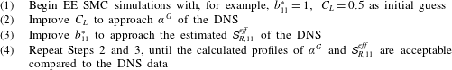
4.2 Closure for the case SmMany

Figure 5.

Mean flow statistics from the present EE SMC and DNS data for the case SmMany: (a) gas void fraction; (b) liquid streamwise velocity and gas streamwise velocity.

For the case SmMany, the procedure of table 2 yields $C_{L}=0.06$ and $b_{11}^{\ast }=1.8$. The results obtained with these values match the DNS data very well. The void fraction in figure 5(a) is identical in the centre and only the near-wall peaks are somewhat more rounded. The mean velocities of gas and liquid also agree very well. Very close to the wall the DNS data exhibit a discretization phenomenon as the gas velocity was determined for the centre of the bubbles, which is at least the bubble radius off the wall. Figure 6 shows that also the Reynolds stresses from the EE SMC agree very well with the reference data in the channel centre. It is important to note that there is a factor of approximately eight between the magnitude of the streamwise and the wall-normal fluctuations and another factor of approximately eight to the turbulent shear stress. This very satisfactory agreement validates not only the choice of the iteratively determined model constants but also the functional form (3.22) and all the other ingredients in the model equations (3.10) and (3.13). Indeed, the achievement can be highlighted by comparison with the results obtained using other standard models from the literature under exactly the same conditions. Cokljat et al. (Reference Cokljat, Slack, Vasquez, Bakker and Montante2006) proposed an isotropic BIT source term, i.e.

(4.5)$$\begin{eqnarray}b_{11}^{C}=b_{22}^{C}=b_{33}^{C}=2/3.\end{eqnarray}$$

Colombo & Fairweather (Reference Colombo and Fairweather2015) suggested

(4.6a,b)$$\begin{eqnarray}b_{11}^{CF}=1,\quad b_{22}^{CF}=b_{33}^{CF}=0.5.\end{eqnarray}$$

However, these relations do not account for the influence of the bubble-induced force field on the pressure–strain correlation (3.20). Their expressions are used here employing the same overall procedure of table 2 for the optimal comparison. It is obvious that, although the shapes of the profiles are similar, the level of the normal stresses is substantially different and bubble-induced anisotropy is not correctly captured.

The reasons for the different behaviour of the BIT models can be seen in the following figures. Using the DNS data, figure 7 shows the essential contributions to the budgets of the Reynolds normal stress $\overline{\overline{u^{\prime }u^{\prime }}}$ with its estimated dissipation term (4.3), modified pressure–strain term (4.2) and effective interfacial term (4.1). Here, the modified pressure–strain term and the dissipation rate constitute the two main sinks for the $\overline{\overline{u^{\prime }u^{\prime }}}$ component. In the channel centre, the budget of $\overline{\overline{u^{\prime }u^{\prime }}}$ reduces to $0\approx \unicode[STIX]{x1D700}_{11}+\unicode[STIX]{x1D719}_{11}^{mod}+\unicode[STIX]{x1D61A}_{R,11}^{eff}$, equation (4.1). This is backed up by figure 7(a), with $\unicode[STIX]{x1D61A}_{R,11}^{eff}$ the dominant source to compensate nearly the sum of the dissipation and the modified pressure–strain. For modelling $\unicode[STIX]{x1D61A}_{R,11}^{eff}$, the target is defined in the core region of the channel as remarked before, since capturing this correctly is a prerequisite for all models. With the present value of $b_{11}^{\ast }$, $\unicode[STIX]{x1D61A}_{R,11}^{SMC\text{-}eff}$ matches the value of the effective interfacial term in the DNS extremely well. The BIT models of Cokljat et al. (Reference Cokljat, Slack, Vasquez, Bakker and Montante2006) and Colombo & Fairweather (Reference Colombo and Fairweather2015) obviously predict significantly lower levels of $\unicode[STIX]{x1D61A}_{R,11}^{eff}$, which in turn leads to the underprediction of $\overline{\overline{u^{\prime }u^{\prime }}}$ and overprediction of $\overline{\overline{v^{\prime }v^{\prime }}}$ observed in figure 6.

Figure 6.

Reynolds-stress components from the present EE SMC and DNS data for the case SmMany: (a) streamwise Reynolds normal stress $\overline{\overline{u^{\prime }u^{\prime }}}$; (b) wall-normal Reynolds normal stress $\overline{\overline{v^{\prime }v^{\prime }}}$; (c) Reynolds shear stress $\overline{\overline{u^{\prime }v^{\prime }}}$. All components are normalized by $U_{b}^{2}$. The label Cokljat refers to EE SMC with $b_{ij}^{C}$ from (4.5), while the label Colombo refers to EE SMC with $b_{ij}^{CF}$ from (4.6) as detailed in the text.

Figure 7.

Comparison of key contributions in the present EE SMC with the DNS data for the case SmMany as described in the text. (a) Selected terms in the budget of $\overline{\overline{u^{\prime }u^{\prime }}}$ with all terms normalized by $U_{b}^{3}/H$. (b) Selected terms in the budget of $\overline{\overline{v^{\prime }v^{\prime }}}$ with all terms normalized by $U_{b}^{3}/H$. (c) Selected terms in the budget of $\unicode[STIX]{x1D700}$ with all terms normalized by $U_{b}^{4}/H^{2}$.

Validating individual terms of the $\unicode[STIX]{x1D700}$ equation (3.13) is not possible since these are not available from the DNS data. Still, some validation can be performed by observing that

(4.7)$$\begin{eqnarray}0\approx \unicode[STIX]{x1D700}_{\unicode[STIX]{x1D700}}+S_{\unicode[STIX]{x1D700}}\end{eqnarray}$$

in the channel centre for the same reasons as with the budget of $\overline{\overline{u^{\prime }u^{\prime }}}$. Hence, $\unicode[STIX]{x1D700}_{\unicode[STIX]{x1D700}}$ can be determined indirectly from the DNS data. For this purpose, it is represented here by the expression

(4.8)$$\begin{eqnarray}\unicode[STIX]{x1D700}_{\unicode[STIX]{x1D700}}=-\unicode[STIX]{x1D6FC}^{L,DNS}C_{\unicode[STIX]{x1D700}2}\frac{(\unicode[STIX]{x1D700}^{DNS})^{2}}{k^{DNS}},\end{eqnarray}$$

using the standard coefficient $C_{\unicode[STIX]{x1D700}2}=1.83$ (Hanjalić & Launder Reference Hanjalić and Launder2011). Equation (4.7) then results in an expression for $S_{\unicode[STIX]{x1D700}}$, with $S_{\unicode[STIX]{x1D700}}=-\unicode[STIX]{x1D700}_{\unicode[STIX]{x1D700}}$. Figure 7(c) shows that the modelled BIT source of the $\unicode[STIX]{x1D700}$ equation, $S_{\unicode[STIX]{x1D700}}^{SMC}$, indeed, provides a very accurate result.

Note, as an aside, that figure 7(b), depicting the dominant components of the budget of the Reynolds normal stress $\overline{\overline{v^{\prime }v^{\prime }}}$, confirms the discussion on the determination of $b_{ij}^{\ast }$, $i=j$, above. Here, the value $b_{22}^{\ast }=0.1$ is obtained not from matching $\unicode[STIX]{x1D61A}_{R,22}^{eff}$, but rather by imposing $b_{ii}^{\ast }=2$ and $b_{22}^{\ast }=b_{33}^{\ast }$, resulting in $b_{22}^{\ast }=\frac{1}{2}(2-b_{11}^{\ast })$. It is worth underlining that the increase in $\overline{\overline{v^{\prime }v^{\prime }}}$ is due to energy being extracted from the $\overline{\overline{u^{\prime }u^{\prime }}}$ component and fed to the $\overline{\overline{v^{\prime }v^{\prime }}}$ component by pressure–strain interaction. Here, in contrast to the $\overline{\overline{u^{\prime }u^{\prime }}}$ component, the modified pressure–strain term, $\unicode[STIX]{x1D719}_{22}^{mod}$, appears as a source in the budget for $\overline{\overline{v^{\prime }v^{\prime }}}$, and the corresponding effective interfacial term $\unicode[STIX]{x1D61A}_{R,22}^{eff}$ exhibits very small influence in the centre.

4.3 Closure for the other monodisperse channel flow cases

Figure 8.

Gas void fraction and Reynolds-stress components from the present EE SMC and DNS data for the other two monodisperse cases: (a,b) SmFew; and (c,d) LaMany.

The procedure of table 2 is now employed for the other two monodisperse bubble-laden channel flows of table 1, namely the cases SmFew and LaMany. Overall, this procedure achieves good agreement for the gas void fraction (figure 8a,c), the Reynolds stresses away from the wall (figure 8b,d) and the other parameters (not shown here to avoid redundancy), yielding the corresponding values of $b_{11}^{\ast }$ and $C_{L}$ reported in table 3. Close to the walls, the Reynolds normal stress profiles are underpredicted by the present SMC computations. This deficiency remains for description of channel flows that are intrinsic to high-$Re$ RANS models for both single-phase (Hanjalić & Launder Reference Hanjalić and Launder1976; Wilcox Reference Wilcox1998) and multiphase flows (Ma Reference Ma2017), and, hence, cannot be overcome by the mere introduction of a more complex BIT model.

4.4 Closure for bidisperse case

In particular for the case BiDisp, it is important to reproduce the profiles of the gas void fraction for smaller bubbles and larger bubbles, individually, not only the profile of the total gas void fraction. This requires that the simulation should be run with different momentum equations describing the predefined gas groups, one group for the smaller bubbles and the other for the larger bubbles. The EE BIT modelling for BiDisp is performed as described in § 3.5 with linear superposition of the BIT source term for each gas group, in both $\unicode[STIX]{x1D61A}_{R,ij}^{SMC\text{-}eff}$ (3.24) and $\unicode[STIX]{x1D61A}_{\unicode[STIX]{x1D700}}^{SMC}$ (3.25).

Figure 9.

(a) Gas void fraction and (b) Reynolds-stress components from the present EE SMC and DNS data for the case BiDisp.

Table 3.

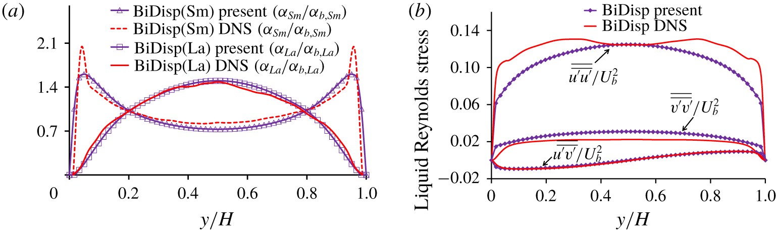
Values of $b_{11}^{\ast }$ and $C_{L}$ obtained by the iterative process for all cases.

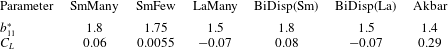
The interfacial force setting follows § 4.1 and the optimization procedure (table 2) is carried out separately for each phase. In particular, the drag coefficients for small and large bubbles are calculated separately using (4.4) based on DNS data for each bubble size and the lift coefficients $C_{L}$ are adjusted to fit the void fraction profiles for smaller and larger bubbles, individually (figure 9a). The agreement achieved in the two void fractions is very good (figure 9a), so that also the total void fraction is well matched (not shown here). The good results for the Reynolds stresses (figure 9b) confirm that the BIT modelling according to § 3.5 is valid also for this bidisperse case. The corresponding values of $b_{11}^{\ast }$ and $C_{L}$ are listed in table 3 as well, together with those of the other three monodisperse cases.

4.5 A case without bulk velocity

Figure 10.

Comparison of the present SMC with experimental data of Akbar et al. (Reference Akbar, Hayashi, Hosokawa and Tomiyama2012): (a) gas void fraction, (b) liquid streamwise velocity and gas streamwise velocity, (c) liquid Reynolds normal stresses and (d) liquid Reynolds shear stress.

To enhance the dataset over a wider range of bubble Reynolds numbers, further experimental data are used for a case that is characterized by the dominance of BIT as well, here the case reported by Akbar et al. (Reference Akbar, Hayashi, Hosokawa and Tomiyama2012). The Akbar case features a rectangular water–air bubble column, with a gas superficial velocity of $3~\text{mm}~\text{s}^{-1}$. Its height $(x)$, width $(y)$ and depth $(z)$ are 800 mm, 240 mm and 72 mm, respectively. Here, the coordinate system of the previous cases is used for improved readability, which is different from the one employed in the original paper. The global gas void fraction is 1.285 %, which is around half of the value in the case SmMany. However, the bubble diameter is much larger. Furthermore, this case is very close to monodisperse with $d_{p}=4.37~\text{mm}$ (Akbar et al. Reference Akbar, Hayashi, Hosokawa and Tomiyama2012). More details are provided in the cited reference.

The present EE SMC simulation was performed on a $175\times 240\times 36$ grid in the $x$-, $y$- and $z$-directions, respectively. Based on our own previous work, the same set of interfacial force models as detailed by Liao et al. (Reference Liao, Ma, Krepper, Lucas and Fröhlich2019) were employed to achieve good agreement of gas void fraction and relative velocity. However, the experimental database does not provide any information about budgets of turbulence parameter, so that the procedure of table 2 cannot be applied directly here to yield $b_{11}^{\ast }$. Instead, this is achieved by adjustments of $b_{11}^{\ast }$ in the source term to match the Reynolds stresses measured in the experiment. Such a procedure is allowed for the present BIT closure at second-moment level for the following reason. If the complete set of the SMCs (six Reynolds-stress equations and one dissipation equation) for a BIT-dominated flow are fixed, with $b_{11}^{\ast }$ the only unknown, since $b_{22}^{\ast }=b_{33}^{\ast }=\frac{1}{2}(1-b_{11}^{\ast })$ is imposed, there appears to be only one value of $b_{11}^{\ast }$. For the Akbar case this procedure yields the value $b_{11}^{\ast }=1.4$ suitable to fit the resulting Reynolds stress $\overline{\overline{u^{\prime }u^{\prime }}}$. Since the form of the BIT source in the $\unicode[STIX]{x1D700}$ equation is fixed, this results in corresponding fixed $\unicode[STIX]{x1D700}_{ij}$ in the Reynolds-stress equations.

Note that the present approach is exempt from the pitfalls identified by the two-equation RANS model using ad hoc models targeting TKE only. The key difference is that there the BIT source of the $\unicode[STIX]{x1D700}$ equation is not fixed as detailed in Ma et al. (Reference Ma, Santarelli, Ziegenhein, Lucas and Fröhlich2017). Figure 10(a,b) shows a comparison of the simulated and experimental gas distribution, vertical liquid velocity and vertical gas velocity. All profiles were taken along the measurement line from the wall to the centre (half the column width) at a height of 500 mm in the midplane ($z=36~\text{mm}$). The agreement of the mean flow profiles obtained with the present SMC closure is very satisfactory and improves substantially upon other models, such as our own previous work (Ma et al. Reference Ma, Ziegenhein, Lucas, Krepper and Fröhlich2015b). The flatter profile for the liquid velocity in figure 10(b) may be due to the slight inaccuracy in the gas void fraction close to the wall and using the high-$Re$ SMC version. Concerning the liquid Reynolds stresses, the present BIT model provides accurate results, reproducing the ratio of the Reynolds normal stresses $\overline{\overline{u^{\prime }u^{\prime }}}:\overline{\overline{v^{\prime }v^{\prime }}}\sim 2.5:1$ observed in the experiment for the centre region of the measurement line, as shown in figure 10(c,d).

5.1 Anisotropy invariants

It is common practice when developing SMC models to analyse the anisotropy of the flows. As argued by Lumley & Newman (Reference Lumley and Newman1977), the local state of the Reynolds-stress anisotropy tensor $\unicode[STIX]{x1D622}_{ij}$ can be usefully characterized by its second ($A_{2}=\unicode[STIX]{x1D622}_{ji}\unicode[STIX]{x1D622}_{ij}$) and third ($A_{3}=\unicode[STIX]{x1D622}_{ij}\unicode[STIX]{x1D622}_{jk}\unicode[STIX]{x1D622}_{ki}$) invariants. These two anisotropy invariants can certainly be combined in various ways to generate further invariants, for example, a useful third norm, known as Lumley’s flatness parameter (Lumley Reference Lumley1978),

(5.1)$$\begin{eqnarray}A=1-9(A_{2}-A_{3})/8.\end{eqnarray}$$

In isotropic turbulence, both $A_{2}$ and $A_{3}$ vanish, and $A=1$. The other extreme condition corresponds to the two-component limit, where $A_{2}=A_{3}+8/9$, so that $A=0$.

Figure 11.

Anisotropy invariants: (a) the single-phase case Unladen; and (b) the case SmMany.

To give some impression of how the above invariants may be distributed in a bubbly flow, figure 11 shows a comparison between the case SmMany and the case Unladen, both obtained from the DNS data. The flatness parameter $A$ vanishes at the wall in both cases as turbulence is in the two-component limit for geometrical reasons. In contrast to the single-phase situation, when $A$ increases towards the centre and approaches unity, the value of $A$ is around $0.25$ almost over the entire channel in the case SmMany, indicating a very anisotropic turbulence state that is generated by the bubbles. This state can also be identified by a much larger second invariant $A_{2}$ observed in this case, which gives a direct measure of the magnitude of the stress anisotropy. The third invariant $A_{3}$ has a similar behaviour as the corresponding value of $A_{2}$ in both cases and broader flatter profiles are observed in the SmMany case. Similar trends as for SmMany are identified in the other bubble-laden cases as well (not shown here), implying a very different nature of stress anisotropy compared to the corresponding single-phase flow.

For a more detailed analysis, it was shown by Lumley & Newman (Reference Lumley and Newman1977) that the realizable states for the stress anisotropy $\unicode[STIX]{x1D622}_{ij}$ should satisfy the following inequalities:

(5.2)$$\begin{eqnarray}6^{1/3}{|A_{3}|}^{2/3}\leqslant A_{2}\leqslant {\textstyle \frac{8}{9}}+A_{3}.\end{eqnarray}$$

These inequalities give rise to the anisotropy-invariant map shown in figure 12. The upper line corresponds to the two-component limit (the last equality in (5.2)), the left-hand line to the axisymmetric contraction limit (the first equality in (5.2), with $A_{3}<0$), and the right-hand line to the axisymmetric expansion limit (the first equality in (5.2), with $A_{3}>0$).

Figure 12.

Anisotropy-invariant map of the DNS data for all cases considered. (a) The cases SmMany, LaMany, BiDisp and Akbar; $Re_{p}$ of the case BiDisp is calculated from the averaged $u_{r}$ and the averaged $d_{p}$ from the DNS of BiDisp. (b) The case SmFew and (c) the single-phase case Unladen.

Figure 12 shows the points for $\unicode[STIX]{x1D622}_{ij}$ derived from DNS and experiment on the anisotropy-invariant map for different $y^{+}$ positions over all the cases considered (the centre point of the measurement line is plotted for the Akbar case). Profiles for the bubble-laden cases and the single-phase case are plotted separately for better comparison. Additionally, the points obtained from the case SmFew would overlap the points from SmMany, so that it is plotted in figure 12(b) separately, as well. A first observation is that all states from both single-phase and bubbly flows, indeed, stay within the Lumley triangle, as is required by realizability constraints. The main difference between the two is that the path crosses the channel in the wall-normal direction. Among them, the Unladen case (figure 12c) shows a traverse from the wall towards the channel centre – starting in the two-component limit, progressing along the axisymmetric expansion line, and ending in the vicinity of the point $A_{2}=A_{3}=0$, which corresponds to isotropic turbulence. In contrast, the present bubbly flows achieve a general trend that they begin from the two-component limit at the wall, traverse with a relatively short path, and then directly end very close to the axisymmetric expansion limit. Moreover, most points aggregate close to this right-hand line to axisymmetric limit for the bubble-laden DNSs, quite the opposite of what is found in the single-phase channel. The origin of this difference is due to the dominant streamwise velocity fluctuations (see figures 6, 8b, 8d and 9b) compared to the other two directions over a large range of the channel centre for the bubble-laden cases. Such a major contribution of normal stress in the streamwise direction was also found by a recent DNS study by du Cluzeau, Bois & Toutant (Reference du Cluzeau, Bois and Toutant2019), who considered this feature later in an algebraic expression for BIT.

Another important observation can be made about the locations of the points aggregated close to the line corresponding to the axisymmetric expansion limit for each particular bubble-laden case. These points are from the centre region of the channel as remarked before; the points distribution on this right-hand limit line towards the isotropic point – direction decreasing with $A_{2}$ – is in the sequence SmMany (SmFew), BiDisp, LaMany to Akbar, which corresponds to increasing bubble Reynolds number, $Re_{p}$, as illustrated in figure 12(a,b). This interesting finding can also be identified by figures 6, 8(b), 8(d), 9(b) and 10, with a gradually less dominant streamwise Reynolds normal stress for theses cases in the order mentioned above. The trend reflects that $Re_{p}$ appears to have a decisive effect on the anisotropy state of the BIT-dominated flows. Such an effect may originate from two parts: the $Re_{p}$-dependent wake structure (see the supplementary material to Santarelli & Fröhlich (Reference Santarelli and Fröhlich2016)) and the path of the rising bubbles (Horowitz & Williamson Reference Horowitz and Williamson2010; Ern et al. Reference Ern, Risso, Fabre and Magnaudet2012).

5.2 The model and its realizability

Figure 13.

Values of $b_{11}^{\ast }$ as a function of $Re_{p}$ for all cases considered. The dashed line shows the fit.

The final step is to propose a general model for the BIT terms. Based on previous experience, this is done by providing a functional relation for the coefficient $b_{11}^{\ast }$. The important observation in § 5.1 that the magnitude of anisotropy decreases with the bubble Reynolds number suggests modelling $b_{11}^{\ast }$ as a function of $Re_{p}$. Pairs of discrete values of $b_{11}^{\ast }$ and $Re_{p}$ are displayed in figure 13. For the case BiDisp, two data points are plotted, one for the smaller bubbles and one for the larger bubbles, with the assumption that the contributions from the two bubble sizes sum up to the total contribution as discussed in § 4.4. Obviously, $b_{11}^{\ast }$ decreases with $Re_{p}$ – implying a trend towards more isotropy, which supports the observations made before. Hence, an expression for $b_{11}^{\ast }$ as a function of $Re_{p}$ seems suitable to generate a model for $\unicode[STIX]{x1D61A}_{R,ij}^{eff}$. By curve fitting (figure 13), the following effective BIT source was determined:

(5.3)

Here $b_{11}^{\ast }\leqslant 2$ is imposed to fulfill $b_{ii}^{\ast }=2$ and $b_{22}^{\ast }=b_{33}^{\ast }\geqslant 0$. The above expression for $b_{11}^{\ast }$ included in figure 13 provides an excellent approximation for the results over the range considered in the available data with a maximum deviation of 1.6 % at the data points. In the limit of high particle Reynolds number, the expression for $b_{11}^{\ast }$ in (5.3) approaches the value $1.34$, which implies that the Reynolds-stress anisotropy does not change much when reaching a certain $Re_{p}$ (recall that for $Re_{p}=1080$ in the case Akbar $b_{11}^{\ast }=1.4$). This is reasonable on the background of an axisymmetric wake embedded in turbulence at high enough particle Reynolds number (Bagchi & Balachandar Reference Bagchi and Balachandar2004; Rind & Castro Reference Rind and Castro2012). The former observed a ratio of the streamwise velocity fluctuation to the cross-streamwise velocity fluctuation of approximately $1.4$ for $Re_{p}=610$. That is similar to the ratio of approximately $1.3$ obtained by the latter (Rind & Castro Reference Rind and Castro2012) for an axisymmetric wake with an equivalent $Re_{p}$ (based on the wake half-width and the centreline deficit velocity) in excess of $10\,000$. Here, the relatively small change of this ratio over a large range of $Re_{p}$ supports an almost constant value for $b_{11}^{\ast }$ appearing in the source for the Reynolds-stress anisotropy at relatively large $Re_{p}$. However, the absolute values obtained by Bagchi & Balachandar (Reference Bagchi and Balachandar2004) and Rind & Castro (Reference Rind and Castro2012) cannot be directly used for correlation, since in the present study bubble swarms are considered. It might appear more direct to construct an expression for $b_{11}^{\ast }$ as a function of $A_{2}$ and $A_{3}$. Such stress invariants find many uses in SMC for single-phase flows (e.g. by Launder & Li Reference Launder and Li1994; Ristorcelli et al. Reference Ristorcelli, Lumley and Abid1995; Jakirlić & Hanjalić Reference Jakirlić and Hanjalić2002). However, this provides pitfalls for modelling $\unicode[STIX]{x1D61A}_{R,ij}^{SMC\text{-}eff}$ in bubbly flows, e.g. in cases when bubbles rise in a highly turbulent background flow. In this situation, $A_{2}$ represents both the property of the background flow as well as the property of the BIT. In contrast, the present $Re_{p}$-dependent expression for $b_{11}^{\ast }$ avoids such a pitfall.

Figure 14.

Anisotropy-invariant map of the present SMC for all bubble-laden cases considered.

Figure 14 shows the anisotropy-invariant map with the points derived from the EE SMC simulations. All points lie within the triangular domain, indicating that the present EE SMC employed with (5.3) provides realizable results for all the cases. Moreover, it is interesting to compare the results of the SMC with the DNS in figure 12. The assumption $b_{22}=b_{33}$, which results in $b_{22}^{\ast }=b_{33}^{\ast }$ as described in § 3.4, imposes that the results of the EE SMC yield axisymmetric turbulence in BIT-dominated cases. The DNS show that in all cases there are several points very close to the two-component limit. These points correspond to the viscous sublayer that is closest to the wall. As mentioned before, the present EE SMC in a high-$Re$ version is not intended to capture this near-wall region, hence, the two-component limit is not approached. Going further away from the wall, the model results follow the same $Re_{p}$-dependent trend as observed by DNS along the axisymmetric expansion line very well, within reasonable tolerance in the absolute values of the stress invariants.