


1 Introduction
Shock wave–boundary layer interactions (SWBLI) play a critical role in the design process of many aspects of transonic or supersonic flight vehicles. They may be encountered in supersonic inlets, in compressor and turbine cascades, on transonic wings and in a large number of other situations relevant to the high-speed flight regime. These interactions can bring about undesirable features, such as increased pressure losses, flow unsteadiness and localized heat loads. Many of these features are directly associated with the occurrence of flow separation (Dolling Reference Dolling2001). The two dominant parameters determining the severity of the interaction are the strength of the shock wave and the state of the incoming boundary layer (laminar/transitional/turbulent). Since turbulent interactions are more commonly encountered for the Reynolds number regime of typical flight conditions (Babinsky & Harvey Reference Babinsky and Harvey2011) most researchers have focussed their attention to this particular type of interaction. However, with the economic and environmental challenges facing the aerospace sector there has been an ongoing effort for achieving laminar flow on both the internal and external components of air and spacecraft. Laminar/transitional SWBLI are therefore expected to become more prevalent in the decades to come and additional research is needed on the potential drawbacks of these interactions when compared to turbulent ones.
A sketch of an oblique shock wave reflection with a laminar incoming boundary layer and transition in the rear part of the bubble (a); the corresponding pressure distribution (b). The sketch is inspired by the studies of previous workers in the field (Gadd, Holder & Regan Reference Gadd, Holder and Regan1954; Chapman, Kuehn & Larson Reference Chapman, Kuehn and Larson1957; Hakkinen et al. Reference Hakkinen, Greber, Trilling and Abarbanel1959; Le Balleur & Délery Reference Le Balleur and Délery1973) and by the results obtained in this paper.

It is well known that laminar boundary layers are more prone to separation than turbulent boundary layers. Gadd et al. (Reference Gadd, Holder and Regan1954) were among the first workers to experimentally investigate laminar, transitional and turbulent interactions. From Schlieren visualizations and pressure measurements, they found that the laminar interaction exhibits an elongated, flat separation bubble which extends both far upstream and downstream of the impinging shock wave. The separation bubble has an approximately triangular shape and acts as a ramp for the incoming flow, creating a series of weak compression waves upstream of the incident shock wave. The boundary layer is lifted over the bubble and continues nearly unaltered when moving downstream (Hakkinen et al. Reference Hakkinen, Greber, Trilling and Abarbanel1959; Reyhner & Flügge-Lotz Reference Reyhner and Flügge-Lotz1968). The incident shock reflects as an expansion wave from the top of the separation bubble shear layer, and at reattachment, again a series of compression waves is created. This process is schematically presented in figure 1, which shows both the interaction flow topology and the corresponding pressure distribution.
The process of boundary layer separation for laminar SWBLIs can be characterized by the free interaction theory (Chapman et al. Reference Chapman, Kuehn and Larson1957), which states that the initial separation process depends only upon upstream flow properties and not on the downstream flow conditions. The initial pressure rise throughout the interaction should therefore, in principle, be independent of the shock strength and the type of interaction (e.g. oblique shock wave reflections or compression corner). Free interactions are the result of a mutual interaction between the viscous boundary layer and the inviscid free stream. That is, a pressure rise in the free stream leads to a thickening of the boundary layer and a thickening of the boundary layer again leads to a compression of the free stream. At some point a stable situation is obtained, in which the pressure rise in the free stream is balanced by the frictional effects in the thickening boundary layer.
For weak shock waves and low Reynolds number, it is possible for the boundary layer to remain laminar throughout the entire interaction region. The work of Le Balleur & Délery (Reference Le Balleur and Délery1973), however, showed that for interactions with a laminar incoming boundary layer, the transition front gradually moves upstream when increasing the shock strength. The shock strength is typically expressed as the ratio of the pressure $p_{3}$
downstream of the interaction versus the upstream pressure
$p_{3}$
downstream of the interaction versus the upstream pressure $p_{1}$
(see also figure 1). For pressure jumps
$p_{1}$
(see also figure 1). For pressure jumps $p_{3}/p_{1}$
larger than 1.4, they found that, independent of the Reynolds number, transition sets in at the impingement point of the incident shock. A mixed type of interaction is therefore obtained, with a laminar boundary layer upstream of the shock and the downstream part of the interaction exhibiting a transitional behaviour.
$p_{3}/p_{1}$
larger than 1.4, they found that, independent of the Reynolds number, transition sets in at the impingement point of the incident shock. A mixed type of interaction is therefore obtained, with a laminar boundary layer upstream of the shock and the downstream part of the interaction exhibiting a transitional behaviour.
The size of the separation bubble for both type of interactions shows a near-linear dependence with the driving pressure coefficient (pressure jump minus pressure required for incipient separation) and the local displacement thickness (Gadd et al. Reference Gadd, Holder and Regan1954; Hakkinen et al. Reference Hakkinen, Greber, Trilling and Abarbanel1959; Katzer Reference Katzer1989). Typically, researchers have recorded only weak Reynolds number effects on the size of the separation bubble (Gadd et al. Reference Gadd, Holder and Regan1954; Hakkinen et al. Reference Hakkinen, Greber, Trilling and Abarbanel1959; Katzer Reference Katzer1989). For a fully laminar interaction, the separation bubble is found to increase in size with Reynolds number, while for the mixed type of interaction, a reverse trend is observed.
This mixed type of interaction was investigated in more detail in the numerical work of Teramoto (Reference Teramoto2005), Sansica, Sandham & Hu (Reference Sansica, Sandham and Hu2014), Larchevêque (Reference Larchevêque2016) and the experimental work of Diop, Piponniau & Dupont (Reference Diop, Piponniau and Dupont2016). The latter performed hot-wire anemometry measurements to quantify the unsteadiness of an oblique shock wave reflection with a laminar incoming boundary layer at a Mach number of 1.68, unit Reynolds number of $11\times 10^{6}~\text{m}^{-1}$
and a flow deflection angle of
$11\times 10^{6}~\text{m}^{-1}$
and a flow deflection angle of $\unicode[STIX]{x1D703}=6^{\circ }$
. The hot-wire was located outside of the boundary layer and recorded the pressure waves radiated from the boundary layer developing over the shock-induced separation bubble. At the interaction onset a temporary amplification in the low-frequency disturbances is recorded, indicative of the breathing nature of the separation bubble. The high-frequency disturbances are also amplified at the interaction onset and stay at an elevated level throughout the interaction. The boundary layer appears to stay in a laminar state over most of the pressure plateau, with transition setting in just before the shock impingement location, resulting in an amplification of both the low- and high-frequency disturbances.
$\unicode[STIX]{x1D703}=6^{\circ }$
. The hot-wire was located outside of the boundary layer and recorded the pressure waves radiated from the boundary layer developing over the shock-induced separation bubble. At the interaction onset a temporary amplification in the low-frequency disturbances is recorded, indicative of the breathing nature of the separation bubble. The high-frequency disturbances are also amplified at the interaction onset and stay at an elevated level throughout the interaction. The boundary layer appears to stay in a laminar state over most of the pressure plateau, with transition setting in just before the shock impingement location, resulting in an amplification of both the low- and high-frequency disturbances.
Similar results were also noted in the numerical study of Larchevêque (Reference Larchevêque2016). Large eddy simulations (LES) furthermore revealed a clear connection between the perturbations present in the incoming laminar boundary layer and the size of the separation bubble. Strong inflow perturbations result in boundary layer transition before reaching the incident shock wave, thus causing extra mixing and a shorter separation bubble. It was noted that the bubble size is approximately halved when increasing the amplitude of the inflow perturbations by a factor of 32 ( $u_{inflow}^{\prime }/U_{\infty }=0.0026\,\%$
to 0.082 %).
$u_{inflow}^{\prime }/U_{\infty }=0.0026\,\%$
to 0.082 %).
In a recent study by the authors (Giepman, Schrijer & Van Oudheusden Reference Giepman, Schrijer and Van Oudheusden2015) high-resolution particle image velocimetry (PIV) measurements were performed on transitional oblique shock wave reflections for a Mach number of 1.7, unit Reynolds number of $35\times 10^{6}~\text{m}^{-1}$
and a flow deflection angle of
$35\times 10^{6}~\text{m}^{-1}$
and a flow deflection angle of $\unicode[STIX]{x1D703}=3^{\circ }$
(
$\unicode[STIX]{x1D703}=3^{\circ }$
( $p_{3}/p_{1}=1.35$
). A full-span flat-plate model was used to generate a laminar boundary layer, while a partial-span shock generator was used to position the oblique shock wave in either the laminar, transitional or turbulent part of the boundary layer. The same configuration and wind tunnel has also been used in the current study.
$p_{3}/p_{1}=1.35$
). A full-span flat-plate model was used to generate a laminar boundary layer, while a partial-span shock generator was used to position the oblique shock wave in either the laminar, transitional or turbulent part of the boundary layer. The same configuration and wind tunnel has also been used in the current study.
This earlier study focused mostly on the development of the measurement methodology and the characterization of the natural boundary layer transition process by means of a variety of different measurement techniques. Measuring the laminar boundary layer by means of PIV under these conditions proved to be highly challenging due to the small boundary layer thickness ( ${\sim}$
0.2 mm), the high shear rate (a gradient of
${\sim}$
0.2 mm), the high shear rate (a gradient of ${\sim}$
0.9 pixels of particle displacement per pixel in the wall-normal direction) and the highly non-uniform seeding distribution. High-resolution PIV measurements were performed and (pre-) processing techniques were developed to handle these adverse testing conditions. The laminar interaction revealed a long (
${\sim}$
0.9 pixels of particle displacement per pixel in the wall-normal direction) and the highly non-uniform seeding distribution. High-resolution PIV measurements were performed and (pre-) processing techniques were developed to handle these adverse testing conditions. The laminar interaction revealed a long ( ${\sim}100\unicode[STIX]{x1D6FF}_{i,0}^{\ast }$
) and flat separation bubble, with transition setting in right after passing the incident shock wave. Here
${\sim}100\unicode[STIX]{x1D6FF}_{i,0}^{\ast }$
) and flat separation bubble, with transition setting in right after passing the incident shock wave. Here $\unicode[STIX]{x1D6FF}_{i,0}^{\ast }$
refers to the incompressible displacement thickness measured at the interaction onset. The boundary layer was found to recover quickly after passing the shock system and a fully turbulent boundary layer is obtained approximately
$\unicode[STIX]{x1D6FF}_{i,0}^{\ast }$
refers to the incompressible displacement thickness measured at the interaction onset. The boundary layer was found to recover quickly after passing the shock system and a fully turbulent boundary layer is obtained approximately $80{-}90\unicode[STIX]{x1D6FF}_{i,0}^{\ast }$
downstream of the incident shock.
$80{-}90\unicode[STIX]{x1D6FF}_{i,0}^{\ast }$
downstream of the incident shock.
The objective of the current study is to develop an extended experimental database of laminar and transitional oblique shock wave reflections by considering a range of Mach numbers, Reynolds numbers and flow deflection angles, using high-resolution PIV measurements according to the methodologies developed and validated earlier in Giepman et al. (Reference Giepman, Schrijer and Van Oudheusden2015). In contrast to earlier studies in this field, the fact of having full field velocity data available makes it possible to directly study the relation between flow deflection angle, separation bubble size/shape and boundary layer transition location. The process of boundary layer transition is captured by tracking the incompressible shape factor of the detached boundary layer over the separation bubble, clearly indicating its dependency on the flow deflection angle, Mach and Reynolds number.
The database was furthermore used to study the applicability of the free-interaction theory (Chapman et al. Reference Chapman, Kuehn and Larson1957) to weak laminar/transitional interactions. Weak in this context implies that a pressure plateau is not reached. Although the free-interaction theory is properly validated for relatively strong interactions (Delery & Marvin Reference Delery and Marvin1986), where a pressure plateau is established, much less information is available for weak near-incipiently separated interactions. This study, however, shows that the free-interaction theory also provides a good estimate of the initial pressure rise through laminar interactions that do not reach a plateau pressure level.
The organization of the paper is as follows. First a description is provided of the experimental arrangement (§ 2), including the tunnel operating conditions and the PIV set-up. Section 3 presents a short summary of the processing and analysis techniques developed in Giepman et al. (Reference Giepman, Schrijer and Van Oudheusden2015) and § 4 discusses the related uncertainties. The main findings and results are presented and discussed in detail in § 5.
2 Experimental arrangement
2.1 Tunnel operating conditions
The experiments were carried out in the TST-27 blowdown transonic/supersonic wind tunnel of Delft University of Technology. The test section measures $270\times 280~\text{mm}^{2}$
and the tunnel is equipped with a contoured nozzle and adjustable throat, the latter allows for a continuous change of the Mach number. As a baseline configuration, the tunnel was operated at a Mach number of 1.7, a total pressure
$270\times 280~\text{mm}^{2}$
and the tunnel is equipped with a contoured nozzle and adjustable throat, the latter allows for a continuous change of the Mach number. As a baseline configuration, the tunnel was operated at a Mach number of 1.7, a total pressure $p_{0}$
of 2.3 bar and a total temperature
$p_{0}$
of 2.3 bar and a total temperature $T_{0}$
of 278 K with a corresponding unit Reynolds number of
$T_{0}$
of 278 K with a corresponding unit Reynolds number of $35\times 10^{6}~\text{m}^{-1}$
. Additionally measurements were also performed at free stream Mach numbers of:
$35\times 10^{6}~\text{m}^{-1}$
. Additionally measurements were also performed at free stream Mach numbers of: $M=1.6$
, 2.0 and 2.3. The unit Reynolds number for these measurements was kept at
$M=1.6$
, 2.0 and 2.3. The unit Reynolds number for these measurements was kept at $35\times 10^{6}~\text{m}^{-1}$
by changing the total pressure
$35\times 10^{6}~\text{m}^{-1}$
by changing the total pressure $p_{0}$
to 2.2, 2.6 and 3.0 bar for these cases, respectively.
$p_{0}$
to 2.2, 2.6 and 3.0 bar for these cases, respectively.
As this study deals with boundary layer transition, which is critically sensitive to external flow disturbances (Van Driest & Blumer Reference Van Driest and Blumer1962), hot-wire measurements were performed to quantify the free stream turbulence level of the tunnel at the baseline operating conditions ( $M=1.7$
), yielding a root-mean-square (r.m.s.) level on the free stream mass flux of 0.77 %. An analysis of the mass flux spectrum showed that the free stream fluctuations are mostly of an acoustic nature, which allows for a conversion from the mass flux fluctuations to pressure fluctuations (Laufer Reference Laufer1964). The r.m.s. level of the free stream pressure fluctuations was found to be 1.9 % of the free stream static pressure. The exact details of this assessment can be found in Giepman et al. (Reference Giepman, Schrijer and Van Oudheusden2015).
$M=1.7$
), yielding a root-mean-square (r.m.s.) level on the free stream mass flux of 0.77 %. An analysis of the mass flux spectrum showed that the free stream fluctuations are mostly of an acoustic nature, which allows for a conversion from the mass flux fluctuations to pressure fluctuations (Laufer Reference Laufer1964). The r.m.s. level of the free stream pressure fluctuations was found to be 1.9 % of the free stream static pressure. The exact details of this assessment can be found in Giepman et al. (Reference Giepman, Schrijer and Van Oudheusden2015).
Side view (a) and bottom view (b) of the wind tunnel configuration (in grey: flat-plate model, in black: shock generator).

2.2 Wind tunnel models
The experimental set-up consists of two elements, a full-span flat plate with a sharp leading edge ( $R\sim 0.15$
mm), which is used to generate a laminar boundary layer, and a partial-span (64 %) shock generator (see figure 2). The position of the models can be adjusted with respect to each other in streamwise direction, which makes it possible to locate the incident shock wave in the laminar, transitional or turbulent region of the boundary layer, with transition occurring over the range of
$R\sim 0.15$
mm), which is used to generate a laminar boundary layer, and a partial-span (64 %) shock generator (see figure 2). The position of the models can be adjusted with respect to each other in streamwise direction, which makes it possible to locate the incident shock wave in the laminar, transitional or turbulent region of the boundary layer, with transition occurring over the range of $x=55{-}91$
mm (
$x=55{-}91$
mm ( $Re_{x}=1.9\times 10^{6}{-}3.2\times 10^{6}$
).
$Re_{x}=1.9\times 10^{6}{-}3.2\times 10^{6}$
).
Furthermore, the deflection angle $\unicode[STIX]{x1D703}$
of the shock generator can be adjusted, which allows for a study into the effects of shock strength on the SWBLI. Earlier oil flow visualizations (Giepman et al.
Reference Giepman, Schrijer and Van Oudheusden2015) showed that this configuration results in a uniform transition and separation front over regions over
$\unicode[STIX]{x1D703}$
of the shock generator can be adjusted, which allows for a study into the effects of shock strength on the SWBLI. Earlier oil flow visualizations (Giepman et al.
Reference Giepman, Schrijer and Van Oudheusden2015) showed that this configuration results in a uniform transition and separation front over regions over $\pm$
85 and
$\pm$
85 and $\pm$
75 mm with respect to the centreline, respectively. This translates into an aspect ratio of 14 between the width and length of the longest separation bubble (11 mm) recorded in this study. Actually, the aspect ratio exceeds 20 for most of the (weaker) interactions investigated in this study, thus minimizing the effects of three-dimensional flow features on the results recorded along the centreline of the plate.
$\pm$
75 mm with respect to the centreline, respectively. This translates into an aspect ratio of 14 between the width and length of the longest separation bubble (11 mm) recorded in this study. Actually, the aspect ratio exceeds 20 for most of the (weaker) interactions investigated in this study, thus minimizing the effects of three-dimensional flow features on the results recorded along the centreline of the plate.
The models were designed to be as slender as possible to limit blockage and to ensure a steady operation of the wind tunnel. Schlieren visualizations were used to verify that the tunnel was started properly. Figure 3 shows a case where the oblique shock wave is impinging approximately 31 mm from the leading edge of the flat plate, with the tunnel operated at a Mach number of 1.7. The flat plate itself creates a very weak leading edge shock wave ( $\unicode[STIX]{x1D703}\sim 0.1^{\circ }$
), which first reflects on the shock generator and then on the flat plate (sufficiently far downstream of the area of interest for all test conditions).
$\unicode[STIX]{x1D703}\sim 0.1^{\circ }$
), which first reflects on the shock generator and then on the flat plate (sufficiently far downstream of the area of interest for all test conditions).
Schlieren visualization of the wind tunnel configuration ( $M=1.7$
,
$M=1.7$
, $Re_{\infty }=35\times 10^{6}~\text{m}^{-1}$
).
$Re_{\infty }=35\times 10^{6}~\text{m}^{-1}$
).

2.3 Test matrix
A parametric study has been conducted into the effects of the flow deflection angle, Mach number and Reynolds number on laminar/transitional oblique shock wave reflections. As a baseline configuration, a laminar oblique shock wave reflection was investigated for a flow deflection angle of $\unicode[STIX]{x1D703}=3^{\circ }$
, a free stream Mach number of 1.7 and a shock position Reynolds number of
$\unicode[STIX]{x1D703}=3^{\circ }$
, a free stream Mach number of 1.7 and a shock position Reynolds number of $Re_{x_{sh}}=Re_{\infty }\cdot x_{sh}=1.8\times 10^{6}$
,
$Re_{x_{sh}}=Re_{\infty }\cdot x_{sh}=1.8\times 10^{6}$
, $Re_{\infty }$
being the unit length Reynolds number (in
$Re_{\infty }$
being the unit length Reynolds number (in $\text{m}^{-1}$
) and
$\text{m}^{-1}$
) and $x_{sh}$
the shock impingement distance measured from the leading edge of the plate. The effects of the flow deflection angle, Mach number and Reynolds number on the flow field were investigated systematically by changing one parameter at a time and keeping the other parameters fixed (see tables 1–3).
$x_{sh}$
the shock impingement distance measured from the leading edge of the plate. The effects of the flow deflection angle, Mach number and Reynolds number on the flow field were investigated systematically by changing one parameter at a time and keeping the other parameters fixed (see tables 1–3).
Flow deflection angles were tested in the range of $\unicode[STIX]{x1D703}=1^{\circ }{-}5^{\circ }$
, which corresponds to a variation in the inviscid pressure rise over the shock reflection system of
$\unicode[STIX]{x1D703}=1^{\circ }{-}5^{\circ }$
, which corresponds to a variation in the inviscid pressure rise over the shock reflection system of $p_{3}/p_{1}=1.11{-}1.64$
. The Mach number was varied from 1.6 to 2.3 and the shock position Reynolds number
$p_{3}/p_{1}=1.11{-}1.64$
. The Mach number was varied from 1.6 to 2.3 and the shock position Reynolds number $Re_{x_{sh}}$
from
$Re_{x_{sh}}$
from $1.4\times 10^{6}$
to
$1.4\times 10^{6}$
to $3.5\times 10^{6}$
. The Reynolds number variation was accomplished by varying the shock impingement location on the flat plate from
$3.5\times 10^{6}$
. The Reynolds number variation was accomplished by varying the shock impingement location on the flat plate from $x_{sh}=41{-}101$
mm, while keeping the unit Reynolds number at a constant value of
$x_{sh}=41{-}101$
mm, while keeping the unit Reynolds number at a constant value of $Re_{\infty }=35\times 10^{6}~\text{m}^{-1}$
. The boundary layer is laminar for
$Re_{\infty }=35\times 10^{6}~\text{m}^{-1}$
. The boundary layer is laminar for $x_{sh}=41$
and 51 mm, transitional for
$x_{sh}=41$
and 51 mm, transitional for $x_{sh}=61$
, 71, 81 and 91 mm, and turbulent for
$x_{sh}=61$
, 71, 81 and 91 mm, and turbulent for $x_{sh}=101$
mm.
$x_{sh}=101$
mm.
The intermittency levels (time fraction where the flow is turbulent) in tables 1–3 were determined by analysing the seeding distribution in the near-wall region ( $y<0.4\unicode[STIX]{x1D6FF}_{95}$
) of the boundary layer. For laminar boundary layers no seeding is recorded close to the wall, whereas for turbulent flow mixing results in a redistribution of the seeding throughout the whole boundary layer. This approach for characterizing the intermittency level has been further elaborated upon in Giepman et al. (Reference Giepman, Schrijer and Van Oudheusden2015).
$y<0.4\unicode[STIX]{x1D6FF}_{95}$
) of the boundary layer. For laminar boundary layers no seeding is recorded close to the wall, whereas for turbulent flow mixing results in a redistribution of the seeding throughout the whole boundary layer. This approach for characterizing the intermittency level has been further elaborated upon in Giepman et al. (Reference Giepman, Schrijer and Van Oudheusden2015).
Experimental matrix. Flow deflection angle variation.

Experimental matrix Mach number variation.

Experimental matrix Reynolds number variation.

2.4 Particle image velocimetry set-up
The PIV measurements (two-dimensional/two-component) were performed with two Lavision Imager LX cameras, placed on either side of the tunnel. The fields of view ( $12.5\times 5.0~\text{mm}^{2}$
) of the two cameras overlap by approximately 3 mm, to allow for the proper recombination of the images. The cameras have a CCD chip of
$12.5\times 5.0~\text{mm}^{2}$
) of the two cameras overlap by approximately 3 mm, to allow for the proper recombination of the images. The cameras have a CCD chip of $1624\times 1236$
pixels, which is cropped in the wall-normal direction to
$1624\times 1236$
pixels, which is cropped in the wall-normal direction to $1624\times 651$
pixels such that the field of view corresponds with the region of interest. As a side benefit this accelerates the data acquisition by permitting a higher acquisition frequency of 10.2 Hz. The cameras were equipped with a 105 mm micro Nikkor lens
$1624\times 651$
pixels such that the field of view corresponds with the region of interest. As a side benefit this accelerates the data acquisition by permitting a higher acquisition frequency of 10.2 Hz. The cameras were equipped with a 105 mm micro Nikkor lens $f_{\#}=16$
, resulting in a magnification of 0.57 and a spatial resolution of
$f_{\#}=16$
, resulting in a magnification of 0.57 and a spatial resolution of $130~\text{pixels}~\text{mm}^{-1}$
. This resolution corresponds to approximately 26 pixels for a 0.2 mm laminar boundary layer thickness (conditions at
$130~\text{pixels}~\text{mm}^{-1}$
. This resolution corresponds to approximately 26 pixels for a 0.2 mm laminar boundary layer thickness (conditions at $x=40$
mm). In an earlier study by the authors (Giepman et al.
Reference Giepman, Schrijer and Van Oudheusden2015) it was shown that this spatial resolution is sufficient to correctly resolve the laminar boundary layer with an ensemble correlation approach (Meinhart, Wereley & Santiago Reference Meinhart, Wereley and Santiago2000). All settings are summarized in table 4.
$x=40$
mm). In an earlier study by the authors (Giepman et al.
Reference Giepman, Schrijer and Van Oudheusden2015) it was shown that this spatial resolution is sufficient to correctly resolve the laminar boundary layer with an ensemble correlation approach (Meinhart, Wereley & Santiago Reference Meinhart, Wereley and Santiago2000). All settings are summarized in table 4.
Illumination is provided by a double-pulse Nd:YAG Spectra Physics Quanta Ray PIV-400 laser, which is operated at a power of 140 mJ per pulse. The pulse duration is less than 7 ns, which results in a particle displacement during illumination of less than 0.4 pixel and therefore introduces negligible particle blur when considering a diffraction particle size of approximately 3 pixels. The flow was seeded with $\text{TiO}_{2}$
particles (30 nm crystal size), which have a response time of
$\text{TiO}_{2}$
particles (30 nm crystal size), which have a response time of $\unicode[STIX]{x1D70F}_{p}=2.5~\unicode[STIX]{x03BC}\text{s}$
after dehydration (the seeding was heated for 40 min at
$\unicode[STIX]{x1D70F}_{p}=2.5~\unicode[STIX]{x03BC}\text{s}$
after dehydration (the seeding was heated for 40 min at $120\,^{\circ }\text{C}$
before usage). In the region of the incident shock wave this corresponds to a typical relaxation length of 0.7 mm. The response time/length were determined by performing an oblique shock wave test, following the same procedure as outlined by Ragni et al. (Reference Ragni, Schrijer, Van Oudheusden and Scarano2010).
$120\,^{\circ }\text{C}$
before usage). In the region of the incident shock wave this corresponds to a typical relaxation length of 0.7 mm. The response time/length were determined by performing an oblique shock wave test, following the same procedure as outlined by Ragni et al. (Reference Ragni, Schrijer, Van Oudheusden and Scarano2010).
Viewing configuration of the PIV cameras.

3 Data reduction
3.1 PIV pre-processing
The PIV measurements were performed under challenging conditions (thin laminar/transitional boundary layer and relatively low seeding levels near the wall). A correct pre-processing of the raw PIV images is therefore crucial for obtaining accurate velocity data. The pre-processing procedure has been described in detail in Giepman et al. (Reference Giepman, Schrijer and Van Oudheusden2015) and consists of three major steps. First, the raw PIV images are corrected for camera read-out noise. Second, the images are corrected for plate vibrations during the wind tunnel run. The plate vibrates slightly during the experiment (0.03 mm r.m.s.), however, due to the high optical magnification this corresponds to a not insignificant wall displacement of 4 pixels in the images. A correction procedure was therefore implemented that identifies the wall location in every image and then shifts all images to a nominal reference position. Finally, a min–max filtering procedure (6 pixel kernel) is applied to the PIV images to normalize the recorded particle intensities.
3.2 PIV processing
Because of the very thin boundary layer only a limited number of pixels are available that can be used to reconstruct the velocity profile. Therefore elongated interrogation windows of $8\times 96$
pixels stretched along the direction of the wall were used, which corresponds to 0.06 mm in the wall-normal direction and 0.74 mm in the streamwise direction. The overlap was set to 75 % both in the wall-normal and streamwise direction, resulting in vector pitches of 0.015 mm and 0.18 mm, respectively.
$8\times 96$
pixels stretched along the direction of the wall were used, which corresponds to 0.06 mm in the wall-normal direction and 0.74 mm in the streamwise direction. The overlap was set to 75 % both in the wall-normal and streamwise direction, resulting in vector pitches of 0.015 mm and 0.18 mm, respectively.
Because of the small height of the interrogation windows and the relatively low seeding density close to the wall, single image pair correlation is not well suited for resolving the boundary layer profile. Instead an ensemble correlation approach (Meinhart et al. Reference Meinhart, Wereley and Santiago2000) was used, which builds up the correlation plane by computing and summing up the correlation maps for all the image pairs gathered per field of view (typically 500 image pairs were acquired per case). The ensemble correlation technique was implemented in an in-house built iterative multi-grid window deformation PIV code Fluere, which is based upon the work of Scarano & Riethmuller (Reference Scarano and Riethmuller2000).
The velocity fields were post-processed with a normalized median filter to remove spurious vectors (Westerweel & Scarano Reference Westerweel and Scarano2005) and vector relocation (Theunissen, Scarano & Riethmuller Reference Theunissen, Scarano and Riethmuller2008) was performed on vectors for which the interrogation window is overlapping the wall mask.
3.3 Extracting boundary layer data from PIV
The PIV velocity fields are used to study the development of the boundary layer throughout the SWBLI. The major complicating factor here is the lack of seeding in the near-wall region ( ${<}0.1$
mm) of the laminar boundary layer. An elaborate description of the seeding conditions of this experiment can be found in an earlier study by the authors (Giepman et al.
Reference Giepman, Schrijer and Van Oudheusden2015). The major findings of this study are summarized in this section to give the reader a good understanding of the seeding difficulties typically encountered in high Reynolds number laminar shock wave–boundary layer experiments.
${<}0.1$
mm) of the laminar boundary layer. An elaborate description of the seeding conditions of this experiment can be found in an earlier study by the authors (Giepman et al.
Reference Giepman, Schrijer and Van Oudheusden2015). The major findings of this study are summarized in this section to give the reader a good understanding of the seeding difficulties typically encountered in high Reynolds number laminar shock wave–boundary layer experiments.
Figure 4 illustrates the average seeding distribution (obtained from 500 snapshots) over the plate for the case of an undisturbed boundary layer with no impinging shock wave, at a free stream Mach number of 1.7. The seeding particles migrate away from the wall close to the leading edge of the flat plate. This effect is attributed to the high local streamline curvature near the leading edge of the plate and the high level of rotation (large $\unicode[STIX]{x2202}u/\unicode[STIX]{x2202}y$
) in the newly formed laminar boundary layer. Since a laminar boundary layer shows virtually no mixing effects, there is no mechanism to redistribute the particles such that the near-wall region remains empty. The gap initially present between the wall and the properly seeded region therefore persists until the moment of boundary layer transition.
$\unicode[STIX]{x2202}u/\unicode[STIX]{x2202}y$
) in the newly formed laminar boundary layer. Since a laminar boundary layer shows virtually no mixing effects, there is no mechanism to redistribute the particles such that the near-wall region remains empty. The gap initially present between the wall and the properly seeded region therefore persists until the moment of boundary layer transition.
However, transition is an intermittent phenomenon and in one snapshot seeding might be present in the near-wall region of the boundary layer, whereas it might be absent again in the next picture. The presence/absence of seeding can therefore be used as indicator for the state of the boundary layer. The seeding distribution was analysed in detail in the work of Giepman et al. (Reference Giepman, Schrijer and Van Oudheusden2015) and was also compared with transition results following from more traditional techniques (infrared thermography, oil flow and schlieren visualizations). This analysis showed that for the baseline flow conditions boundary layer transition starts at $x=55$
mm (
$x=55$
mm ( $Re_{x}=1.9\times 10^{6}$
) and ends at approximately
$Re_{x}=1.9\times 10^{6}$
) and ends at approximately $x=91$
mm (
$x=91$
mm ( $Re_{x}=3.2\times 10^{6}$
). The intermittency level along this distance increases from approximately 0 to 96 % (see also table 3).
$Re_{x}=3.2\times 10^{6}$
). The intermittency level along this distance increases from approximately 0 to 96 % (see also table 3).
Average seeding distribution along the flat plate ( $M=1.7$
). The red line indicates the wall location.
$M=1.7$
). The red line indicates the wall location.

Laminar boundary layer profile at $x=40$
mm (
$x=40$
mm ( $M=1.7$
).
$M=1.7$
).

The laminar boundary layer has a thickness of approximately 0.2 mm at 40 mm from the leading edge. Using the ensemble correlation approach outlined in § 3.2 it is possible to reliably reconstruct the upper 60 % of the boundary layer profile. The resulting profile is presented in figure 5 and compared with the theoretical compressible flat-plate boundary layer solution. The effects of compressibility are taken into account by applying the Illingworth transformation to the incompressible Blasius solution. For $u\leqslant 0.95U_{\infty }$
an excellent agreement is obtained between the experimental data and the theoretical solution. Note here that the theoretical profile has not been fitted or shifted onto the experimental data, but follows directly from theory. For
$u\leqslant 0.95U_{\infty }$
an excellent agreement is obtained between the experimental data and the theoretical solution. Note here that the theoretical profile has not been fitted or shifted onto the experimental data, but follows directly from theory. For $u\geqslant 0.95U_{\infty }$
, a small discrepancy can be observed between the experimental data and the Blasius solution. The theoretical profile quickly reaches its free stream velocity, whereas the experimental data show a longer and smoother transition to the free stream velocity.
$u\geqslant 0.95U_{\infty }$
, a small discrepancy can be observed between the experimental data and the Blasius solution. The theoretical profile quickly reaches its free stream velocity, whereas the experimental data show a longer and smoother transition to the free stream velocity.
Since the experimental results agree well with the theoretical solution, it can be used as a basis to extrapolate the experimental data toward the wall. This approach has been used for calculating, amongst others, the incompressible displacement thickness $\unicode[STIX]{x1D6FF}_{i}^{\ast }$
, the incompressible momentum thickness
$\unicode[STIX]{x1D6FF}_{i}^{\ast }$
, the incompressible momentum thickness $\unicode[STIX]{x1D703}_{i}$
and the incompressible shape factor
$\unicode[STIX]{x1D703}_{i}$
and the incompressible shape factor $H_{i}$
from the experimental data. The boundary layer parameters evaluated at
$H_{i}$
from the experimental data. The boundary layer parameters evaluated at $x=40$
mm are summarized in table 5 and are seen to be in good agreement with the theory.
$x=40$
mm are summarized in table 5 and are seen to be in good agreement with the theory.
Seeding difficulties were also encountered when studying laminar SWBLIs. Figure 6(a) clearly shows that the seeding in the incoming boundary layer is lifted over the separation bubble. Although the situation is slightly alleviated by the presence of a separation bubble, which recirculates a small portion of the particles, the light scattered by the seeding in the bubble remains very low compared with the light coming from the wall reflections. This renders it impossible to obtain reliable velocity data inside the separation bubble, even when using an ensemble correlation approach.
Analysis of the seeding distribution and the reversed flow region for a laminar oblique shock wave reflection ( $M=1.7$
,
$M=1.7$
, $x_{sh}=51$
mm and
$x_{sh}=51$
mm and $\unicode[STIX]{x1D6FF}_{i,0}^{\ast }=0.093$
mm). (a) Seeding distribution; (b) velocity field, the masked white region represents the reversed flow region. (c) Velocity profiles throughout the interaction; symbol definition:
$\unicode[STIX]{x1D6FF}_{i,0}^{\ast }=0.093$
mm). (a) Seeding distribution; (b) velocity field, the masked white region represents the reversed flow region. (c) Velocity profiles throughout the interaction; symbol definition: $\times$
, PIV data; ——, fitted Falkner–Skan velocity profiles; – –, approximated
$\times$
, PIV data; ——, fitted Falkner–Skan velocity profiles; – –, approximated $u=0$
isoline.
$u=0$
isoline.

Boundary layer properties at $x=40$
mm.
$x=40$
mm.

Although the velocity field in the separation bubble cannot be reconstructed from the particle image data, the data further away from the wall ( $u>0.2U_{\infty }$
) can still be considered as reliable, because of the higher seeding density and smaller probability of encountering wall reflections. In the work of Lees & Reeves (Reference Lees and Reeves1964), it was shown that the velocity profiles in the interaction region of a laminar SWBLI may be approximated by Falkner–Skan velocity profiles. It was therefore decided to create a database of Falkner–Skan velocity profiles, containing both separated (lower branch) and attached (upper branch) solutions. These profiles were fitted to the measured velocity profiles in the range from 0.2 to
$u>0.2U_{\infty }$
) can still be considered as reliable, because of the higher seeding density and smaller probability of encountering wall reflections. In the work of Lees & Reeves (Reference Lees and Reeves1964), it was shown that the velocity profiles in the interaction region of a laminar SWBLI may be approximated by Falkner–Skan velocity profiles. It was therefore decided to create a database of Falkner–Skan velocity profiles, containing both separated (lower branch) and attached (upper branch) solutions. These profiles were fitted to the measured velocity profiles in the range from 0.2 to $0.6U_{\infty }$
and were used to approximate the height of the reversed flow region (
$0.6U_{\infty }$
and were used to approximate the height of the reversed flow region ( $u=0$
isoline). This procedure is illustrated in figure 6(c) for a selected number of velocity profiles.
$u=0$
isoline). This procedure is illustrated in figure 6(c) for a selected number of velocity profiles.
An important goal of this study is to track the state of the boundary layer (laminar/transitional/turbulent) developing over the separation bubble. For this purpose an alternative definition of the incompressible shape factor was introduced in the work of Giepman et al. (Reference Giepman, Schrijer and Van Oudheusden2015). In the classical definition of the shape factor, the integration determining the integral boundary layer parameters (displacement and momentum thickness) is performed on the complete velocity profile, from the wall up to the free stream. This implies that the separation bubble will have a major effect on the value of the shape factor, which is undesirable if it is to be used as a metric to indicate transition of the detached boundary layer. Therefore, to eliminate the contribution of the separation bubble to the shape factor, a new ‘artificial’ wall location $y_{aw}$
is defined by linearly extrapolating the velocity profile in the range of
$y_{aw}$
is defined by linearly extrapolating the velocity profile in the range of $0.2{-}0.6U_{\infty }$
to
$0.2{-}0.6U_{\infty }$
to $0~\text{m}~\text{s}^{-1}$
. This implies that the data points below
$0~\text{m}~\text{s}^{-1}$
. This implies that the data points below $y_{aw}$
are therefore no longer used when calculating the shape factor
$y_{aw}$
are therefore no longer used when calculating the shape factor $H_{i,aw}$
. This procedure is illustrated in figure 7 for a velocity profile extracted from a laminar SWBLI case (
$H_{i,aw}$
. This procedure is illustrated in figure 7 for a velocity profile extracted from a laminar SWBLI case ( $\unicode[STIX]{x1D703}=3^{\circ }$
,
$\unicode[STIX]{x1D703}=3^{\circ }$
, $M=1.7$
) at the reattachment location. This newly defined shape factor
$M=1.7$
) at the reattachment location. This newly defined shape factor $H_{i,aw}$
is useful for tracking the state of the boundary layer over the separation bubble and identifying the region of boundary layer transition (Giepman et al.
Reference Giepman, Schrijer and Van Oudheusden2015).
$H_{i,aw}$
is useful for tracking the state of the boundary layer over the separation bubble and identifying the region of boundary layer transition (Giepman et al.
Reference Giepman, Schrijer and Van Oudheusden2015).
Procedure for determining the new ‘artificial’ wall location $y_{aw}$
. The velocity profile has been extracted from a laminar SWBLI (
$y_{aw}$
. The velocity profile has been extracted from a laminar SWBLI ( $M=1.7$
,
$M=1.7$
, $x_{sh}=51$
mm) at the reattachment location (
$x_{sh}=51$
mm) at the reattachment location ( $x-x_{sh}=16\unicode[STIX]{x1D6FF}_{i,0}^{\ast }$
).
$x-x_{sh}=16\unicode[STIX]{x1D6FF}_{i,0}^{\ast }$
).

4 Uncertainty analysis
The PIV measurements are subject to various sources of uncertainty. In this section the dominant sources of uncertainty are identified and their impact on the velocity field, the reversed flow region, the boundary layer shape factor and the wall pressure level is discussed.
4.1 Particle slip and shock smearing
The tracer particles that were used for this experiment have a response time $\unicode[STIX]{x1D70F}_{p}$
of
$\unicode[STIX]{x1D70F}_{p}$
of $2.5~\unicode[STIX]{x03BC}\text{s}$
, which for the laminar flat-plate boundary layer corresponds to a Stokes number of
$2.5~\unicode[STIX]{x03BC}\text{s}$
, which for the laminar flat-plate boundary layer corresponds to a Stokes number of $St=0.1\cdot \unicode[STIX]{x1D70F}_{p}\cdot U_{\infty }/\unicode[STIX]{x1D6FF}_{95}\approx 0.6$
(the factor of 0.1 comes from the definition of Samimy & Lele (Reference Samimy and Lele1991)). This is a high value, which according to the study of Samimy & Lele (Reference Samimy and Lele1991) may result in slip velocities of up to 10 % of the instantaneous local velocity. The present investigation will therefore only address the time-averaged velocity fields and will not deal with the unsteady effects associated with boundary layer transition. Also this means that under the present conditions no meaningful velocity fluctuation statistics can be obtained for the boundary layer and the interaction region. On the mean flow field, particle slip causes a smearing of flow regions that display a high streamwise velocity gradient. The incident shock wave for instance is spread over a region of
$St=0.1\cdot \unicode[STIX]{x1D70F}_{p}\cdot U_{\infty }/\unicode[STIX]{x1D6FF}_{95}\approx 0.6$
(the factor of 0.1 comes from the definition of Samimy & Lele (Reference Samimy and Lele1991)). This is a high value, which according to the study of Samimy & Lele (Reference Samimy and Lele1991) may result in slip velocities of up to 10 % of the instantaneous local velocity. The present investigation will therefore only address the time-averaged velocity fields and will not deal with the unsteady effects associated with boundary layer transition. Also this means that under the present conditions no meaningful velocity fluctuation statistics can be obtained for the boundary layer and the interaction region. On the mean flow field, particle slip causes a smearing of flow regions that display a high streamwise velocity gradient. The incident shock wave for instance is spread over a region of ${\sim}$
2 mm in space, corresponding to
${\sim}$
2 mm in space, corresponding to ${\sim}25\unicode[STIX]{x1D6FF}_{i,0}^{\ast }$
.
${\sim}25\unicode[STIX]{x1D6FF}_{i,0}^{\ast }$
.
4.2 The reversed flow region
The height of the reversed flow region is typically not much more than 0.2 mm, making it sensitive to experimental uncertainties. The three main sources of uncertainty in this respect are: (i) the estimation of the wall location, (ii) cross-correlation noise and (iii) uncertainties coming from the Falkner–Skan extrapolation procedure. These factors will be discussed in this section.
The accuracy with which the wall location can be determined directly affects the accuracy with which the size of the reversed flow region can be determined. As discussed in § 3.1, a method has been developed that identifies the wall location in every PIV image and shifts the images to a nominal reference position. The accuracy of this method is conservatively estimated to be 1 pixel. This corresponds to approximately $8~\unicode[STIX]{x03BC}\text{m}$
, which translates into an uncertainty of
$8~\unicode[STIX]{x03BC}\text{m}$
, which translates into an uncertainty of ${\sim}$
4 % on the height and length of the reversed flow region.
${\sim}$
4 % on the height and length of the reversed flow region.
The velocity fields were constructed by employing the ensemble correlation technique on the PIV dataset (see § 3.2). The laminar/transitional boundary layer displays a high velocity gradient ( ${\sim}$
0.9 pixel/pixel), while seeding conditions are harsh in the near-wall region and aero-optical distortions are present in the vicinity of the shock wave. It is difficult to estimate a priori how these individual factors will influence the reversed flow height determination. So, instead an a posteriori estimate of the r.m.s. uncertainty is given by investigating the amount of scatter on the reversed flow regions, as presented in figure 18(a). Straight lines were fitted to the upstream portion of the reversed flow region and the cross-correlation uncertainty is estimated by calculating the r.m.s. difference between this straight line and the experimental data points. For Mach numbers of 1.6, 1.7, 2.0 and 2.3, uncertainties of, respectively, 2 %, 3 %, 4 % and 6 % with respect to maximum reversed flow height, were recorded. The seeding conditions in the boundary layer deteriorate with increasing Mach number and also the aero-optical distortions were found to become more severe at higher Mach numbers, as such explaining the increased uncertainties for those cases.
${\sim}$
0.9 pixel/pixel), while seeding conditions are harsh in the near-wall region and aero-optical distortions are present in the vicinity of the shock wave. It is difficult to estimate a priori how these individual factors will influence the reversed flow height determination. So, instead an a posteriori estimate of the r.m.s. uncertainty is given by investigating the amount of scatter on the reversed flow regions, as presented in figure 18(a). Straight lines were fitted to the upstream portion of the reversed flow region and the cross-correlation uncertainty is estimated by calculating the r.m.s. difference between this straight line and the experimental data points. For Mach numbers of 1.6, 1.7, 2.0 and 2.3, uncertainties of, respectively, 2 %, 3 %, 4 % and 6 % with respect to maximum reversed flow height, were recorded. The seeding conditions in the boundary layer deteriorate with increasing Mach number and also the aero-optical distortions were found to become more severe at higher Mach numbers, as such explaining the increased uncertainties for those cases.
Due to a very low level of seeding in the near-wall region of laminar separation bubbles it is not possible to determine the size of the reversed flow region ( $u=0$
isoline) directly from the PIV data (see § 3.3). Therefore, as discussed previously, an extrapolation procedure was developed using Falkner–Skan (F–S) velocity profiles to obtain the height of the reversed flow region. F–S velocity profiles have been used before by other researchers (Lees & Reeves Reference Lees and Reeves1964) to approximate the velocity field of laminar SWBLIs, but it remains questionable to what extent they correctly capture the flow field. Within the scope of this work it is important to assess the accuracy with which the height of the reversed flow region can be determined using this F–S extrapolation procedure.
$u=0$
isoline) directly from the PIV data (see § 3.3). Therefore, as discussed previously, an extrapolation procedure was developed using Falkner–Skan (F–S) velocity profiles to obtain the height of the reversed flow region. F–S velocity profiles have been used before by other researchers (Lees & Reeves Reference Lees and Reeves1964) to approximate the velocity field of laminar SWBLIs, but it remains questionable to what extent they correctly capture the flow field. Within the scope of this work it is important to assess the accuracy with which the height of the reversed flow region can be determined using this F–S extrapolation procedure.
Application of the Falkner–Skan fitting procedure and a linear extrapolation procedure to the data of Sansica et al. (Reference Sansica, Sandham and Hu2014). (a) Velocity profiles compared at $x-x_{sh}/\unicode[STIX]{x1D6FF}_{0}^{\ast }=-7$
. (b) Comparison of the
$x-x_{sh}/\unicode[STIX]{x1D6FF}_{0}^{\ast }=-7$
. (b) Comparison of the $u=0$
isolines.
$u=0$
isolines.

It was therefore decided to apply the F–S extrapolation procedure to the direct numerical simulation (DNS) data of Sansica et al. (Reference Sansica, Sandham and Hu2014), who simulated a laminar oblique shock wave reflection ( $\unicode[STIX]{x1D703}=2^{\circ }$
) at a Mach number of 1.5 and Reynolds number of
$\unicode[STIX]{x1D703}=2^{\circ }$
) at a Mach number of 1.5 and Reynolds number of $Re_{x_{sh}}=6.6\times 10^{5}$
. Transition was not modelled in the study of Sansica et al. (Reference Sansica, Sandham and Hu2014) and the mean boundary layer profile thus remains laminar throughout the entire interaction. The reversed flow region is directly available from the numerical data and is compared with the reversed flow region that follows from the F–S extrapolation procedure, again using only the velocity data within the
$Re_{x_{sh}}=6.6\times 10^{5}$
. Transition was not modelled in the study of Sansica et al. (Reference Sansica, Sandham and Hu2014) and the mean boundary layer profile thus remains laminar throughout the entire interaction. The reversed flow region is directly available from the numerical data and is compared with the reversed flow region that follows from the F–S extrapolation procedure, again using only the velocity data within the $0.2{-}0.6U_{\infty }$
velocity range. The separation location and the wall distance of maximum reversed flow are predicted correctly by the F–S extrapolation procedure (see figure 8
b). The height of the reversed flow region is, however, overestimated by
$0.2{-}0.6U_{\infty }$
velocity range. The separation location and the wall distance of maximum reversed flow are predicted correctly by the F–S extrapolation procedure (see figure 8
b). The height of the reversed flow region is, however, overestimated by ${\sim}$
10 % when using the F–S extrapolation procedure. The length of the bubble on the other hand is slightly underestimated by
${\sim}$
10 % when using the F–S extrapolation procedure. The length of the bubble on the other hand is slightly underestimated by ${\sim}$
4 %. These differences can be traced back to the relatively high backflow velocities predicted by the F–S velocity profiles, which are a factor of 2.7 larger than those of the DNS solution (see also figure 8
a). F–S velocity profiles are therefore not well suited to model the details of the (non-similar) flow field inside the separation bubble, but when used as a basis for extrapolation, they can provide a reasonable approximation of the reversed flow height and length.
${\sim}$
4 %. These differences can be traced back to the relatively high backflow velocities predicted by the F–S velocity profiles, which are a factor of 2.7 larger than those of the DNS solution (see also figure 8
a). F–S velocity profiles are therefore not well suited to model the details of the (non-similar) flow field inside the separation bubble, but when used as a basis for extrapolation, they can provide a reasonable approximation of the reversed flow height and length.
It is interesting to notice here that the height and length of the reversed flow region are overestimated by 28 % and ${>}50\,\%$
, respectively, when a simple linear extrapolation is used to reconstruct the
${>}50\,\%$
, respectively, when a simple linear extrapolation is used to reconstruct the $u=0$
isoline. This shows that the more elaborate F–S extrapolation results in substantially lower bias errors (10 % and 4 %, respectively) and is therefore the preferred technique when analysing the reversed flow regions of laminar/transitional interactions. Although Falkner–Skan velocity profiles offer a substantial improvement with respect to a linear extrapolation procedure, it should be emphasized here that Falkner–Skan velocity profiles are essentially only valid for laminar profiles. The method still works for the transitional profiles also encountered in this study, but higher uncertainties are to be anticipated.
$u=0$
isoline. This shows that the more elaborate F–S extrapolation results in substantially lower bias errors (10 % and 4 %, respectively) and is therefore the preferred technique when analysing the reversed flow regions of laminar/transitional interactions. Although Falkner–Skan velocity profiles offer a substantial improvement with respect to a linear extrapolation procedure, it should be emphasized here that Falkner–Skan velocity profiles are essentially only valid for laminar profiles. The method still works for the transitional profiles also encountered in this study, but higher uncertainties are to be anticipated.
4.3 Shape factor development
The incompressible shape factor $H_{i,aw}$
is used in this study as an indicator of the state of the boundary layer (laminar/turbulent) that is developing through the interaction region. The shape factor is subject to three main sources of uncertainty: (i) The estimation of the wall location, (ii) Cross-correlation uncertainty and (iii) uncertainties coming from the extrapolation procedure for the near-wall region.
$H_{i,aw}$
is used in this study as an indicator of the state of the boundary layer (laminar/turbulent) that is developing through the interaction region. The shape factor is subject to three main sources of uncertainty: (i) The estimation of the wall location, (ii) Cross-correlation uncertainty and (iii) uncertainties coming from the extrapolation procedure for the near-wall region.
As discussed in the previous section, the wall location can be estimated with an accuracy of ${\sim}$
1 pixel. For the laminar boundary layer upstream of the interaction (
${\sim}$
1 pixel. For the laminar boundary layer upstream of the interaction ( $x-x_{sh}=-120\unicode[STIX]{x1D6FF}_{i,0}^{\ast }$
,
$x-x_{sh}=-120\unicode[STIX]{x1D6FF}_{i,0}^{\ast }$
, $M=1.7$
) this translates into an uncertainty of 6 % on the incompressible displacement thickness, 3 % on the incompressible momentum thickness and 3 % on the shape factor. For a fully turbulent boundary layer downstream of the interaction (
$M=1.7$
) this translates into an uncertainty of 6 % on the incompressible displacement thickness, 3 % on the incompressible momentum thickness and 3 % on the shape factor. For a fully turbulent boundary layer downstream of the interaction ( $x-x_{sh}=120\unicode[STIX]{x1D6FF}_{i,0}^{\ast }$
,
$x-x_{sh}=120\unicode[STIX]{x1D6FF}_{i,0}^{\ast }$
, $M=1.7$
) this delivers uncertainties of 5 % on the incompressible displacement thickness, 3 % for the momentum thickness and 2 % on the shape factor. The slightly lower uncertainties for the turbulent boundary layer are related to the increased boundary layer thickness, which makes the relative impact of a 1 pixel offset on the integral parameters smaller.
$M=1.7$
) this delivers uncertainties of 5 % on the incompressible displacement thickness, 3 % for the momentum thickness and 2 % on the shape factor. The slightly lower uncertainties for the turbulent boundary layer are related to the increased boundary layer thickness, which makes the relative impact of a 1 pixel offset on the integral parameters smaller.
The value of the shape factor is furthermore affected by cross-correlation uncertainties and errors made when extrapolating the velocity data toward the wall location. The latter is necessary because velocity vectors are never available all the way down to the wall. It is difficult, however, to estimate a priori how these two factors will affect the shape factor. Therefore a similar approach is taken as in the previous section. That is, a smoothing spline is fitted to the data of figure 18(b) and the r.m.s. difference between this spline and the experimental data points is taken as an estimate for cross-correlation and power-law modelling uncertainties. For Mach numbers of 1.6, 1.7, and 2.0 uncertainties of 4 % were recorded on the shape factor. For the $M=2.3$
case slightly higher uncertainties of 6 % were recorded, due to the rather adverse seeding conditions. These uncertainties, although not negligible, are still much smaller than the typical jump in the shape factor observed (
$M=2.3$
case slightly higher uncertainties of 6 % were recorded, due to the rather adverse seeding conditions. These uncertainties, although not negligible, are still much smaller than the typical jump in the shape factor observed ( ${\sim}45$
%) at the point of boundary layer transition (see for example figure 17). The calculated uncertainties are summarized in table 6.
${\sim}45$
%) at the point of boundary layer transition (see for example figure 17). The calculated uncertainties are summarized in table 6.
4.4 Wall pressures from velocity field data
The flow deflection angle $\unicode[STIX]{x1D703}_{flow}=\text{atan}(v/u)$
is used in § 5.3 to convert the velocity field at the onset of the interaction to wall pressure levels. The uncertainty on the flow deflection angle mostly comes from the uncertainty that exists on the location of the correlation peak. This estimate improves when more image pairs are processed with the ensemble correlation technique, but is limited by the finite accuracy of the 3-point Gaussian peak fitting procedure that is used for estimating the location of the correlation peak with sub-pixel accuracy.
$\unicode[STIX]{x1D703}_{flow}=\text{atan}(v/u)$
is used in § 5.3 to convert the velocity field at the onset of the interaction to wall pressure levels. The uncertainty on the flow deflection angle mostly comes from the uncertainty that exists on the location of the correlation peak. This estimate improves when more image pairs are processed with the ensemble correlation technique, but is limited by the finite accuracy of the 3-point Gaussian peak fitting procedure that is used for estimating the location of the correlation peak with sub-pixel accuracy.
An a posteriori approach to determine the corresponding uncertainty is possible by considering the velocity variations in the free stream. In an ideal situation the converged ensemble-averaged velocity in the free stream should yield the same value, small spatial variations with respect to this value can be attributed to the finite accuracy of the peak fitting procedure. The r.m.s. value of the velocity variations is found to be 0.096 % of $U_{\infty }$
or equivalently 0.023 pixels for a dataset of 500 images. This translates into an error on the flow deflection angle of
$U_{\infty }$
or equivalently 0.023 pixels for a dataset of 500 images. This translates into an error on the flow deflection angle of $0.057^{\circ }$
. This uncertainty is reduced further by averaging the calculated flow deflection angles over 25 rows of velocity vectors, in the range of
$0.057^{\circ }$
. This uncertainty is reduced further by averaging the calculated flow deflection angles over 25 rows of velocity vectors, in the range of $5<y/\unicode[STIX]{x1D6FF}_{i,0}^{\ast }<10$
. Assuming the errors on the correlation peaks to be independent across the rows, it can be calculated that the uncertainty on the averaged flow deflection angle equals:
$5<y/\unicode[STIX]{x1D6FF}_{i,0}^{\ast }<10$
. Assuming the errors on the correlation peaks to be independent across the rows, it can be calculated that the uncertainty on the averaged flow deflection angle equals: $0.011^{\circ }$
. This translates into a relative error of 0.7 % on the correlation function
$0.011^{\circ }$
. This translates into a relative error of 0.7 % on the correlation function $F$
presented in figure 20 of this work.
$F$
presented in figure 20 of this work.
Main sources of uncertainty and their impact on our outcomes.

5 Results
5.1 Velocity fields
Figures 9 and 10 present the velocity field in the interaction region for three different flow deflection angles: $\unicode[STIX]{x1D703}=1^{\circ }$
,
$\unicode[STIX]{x1D703}=1^{\circ }$
, $3^{\circ }$
and
$3^{\circ }$
and $5^{\circ }$
. The Mach and Reynolds numbers were fixed at
$5^{\circ }$
. The Mach and Reynolds numbers were fixed at $M=1.7$
and
$M=1.7$
and $Re_{x_{sh}}=1.8\times 10^{6}$
(
$Re_{x_{sh}}=1.8\times 10^{6}$
( $x_{sh}=51$
mm), respectively. A very similar flow topology is recorded for all three interactions. The incident shock wave imposes an adverse pressure gradient which separates the incoming boundary layer. For the
$x_{sh}=51$
mm), respectively. A very similar flow topology is recorded for all three interactions. The incident shock wave imposes an adverse pressure gradient which separates the incoming boundary layer. For the $\unicode[STIX]{x1D703}=1^{\circ }$
case (
$\unicode[STIX]{x1D703}=1^{\circ }$
case ( $p_{3}/p_{1}=1.11$
) the flow is incipiently separated and a small nearly symmetrical separation bubble is formed. The bubble grows in size with increasing flow deflection angle, with the bubble growing mostly in the direction upstream of the incident shock wave. The thickening and subsequent separation of the laminar boundary layer results in the formation of a series of compression waves, which are best visualized in the
$p_{3}/p_{1}=1.11$
) the flow is incipiently separated and a small nearly symmetrical separation bubble is formed. The bubble grows in size with increasing flow deflection angle, with the bubble growing mostly in the direction upstream of the incident shock wave. The thickening and subsequent separation of the laminar boundary layer results in the formation of a series of compression waves, which are best visualized in the $v$
-component of the velocity field (figure 10). The separation bubble reaches its maximum height close to the shock impingement location. From the top of the separation bubble an expansion fan emanates, which deflects the flow towards the surface. Moving further downstream, the boundary layer reattaches again and a series of compression waves is formed.
$v$
-component of the velocity field (figure 10). The separation bubble reaches its maximum height close to the shock impingement location. From the top of the separation bubble an expansion fan emanates, which deflects the flow towards the surface. Moving further downstream, the boundary layer reattaches again and a series of compression waves is formed.
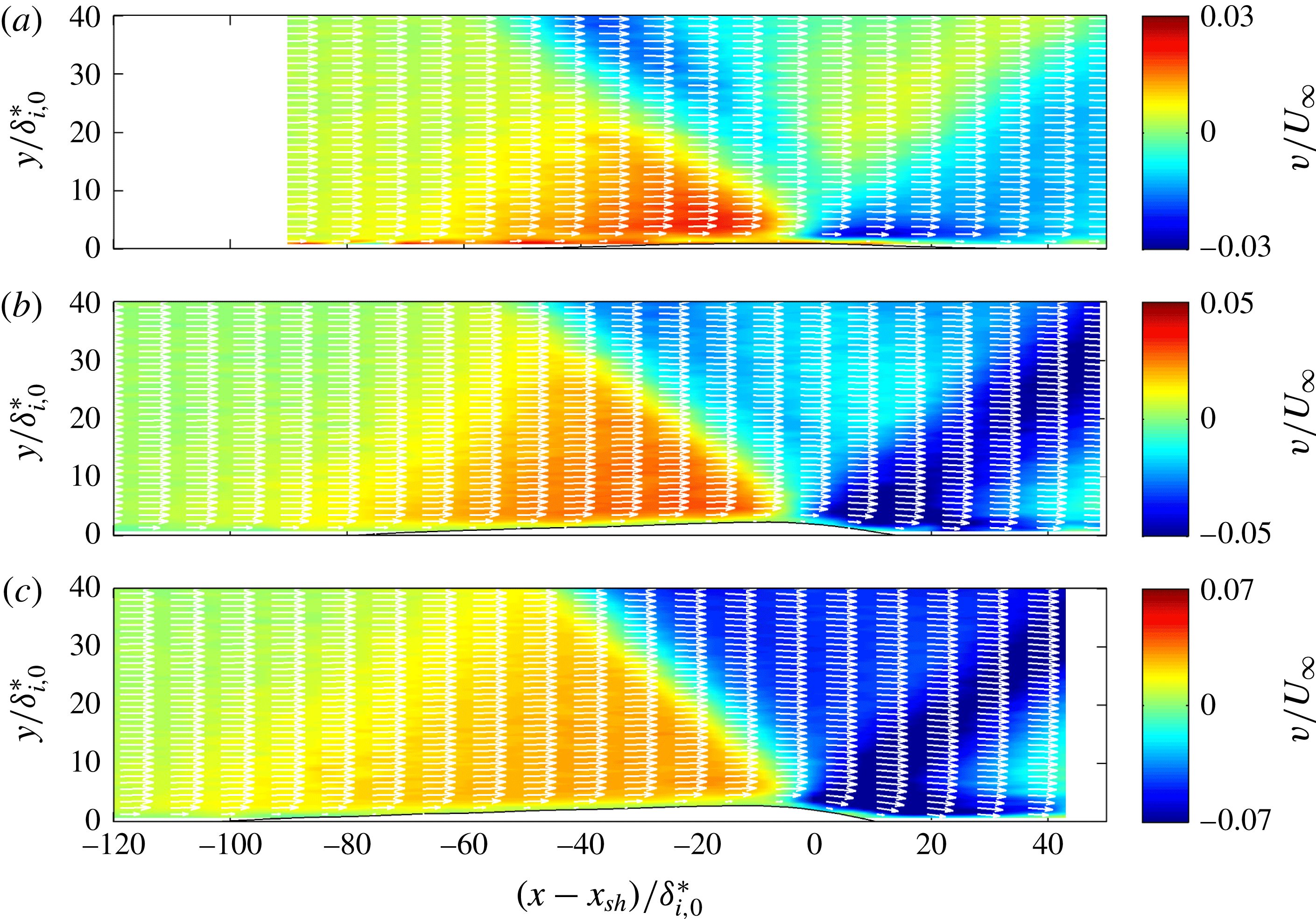
The mean streamwise velocity component for three flow deflection angles. The Mach number and Reynolds number were fixed to $M=1.7$
and
$M=1.7$
and $Re_{x_{sh}}=1.8\times 10^{6}$
, respectively. (a)
$Re_{x_{sh}}=1.8\times 10^{6}$
, respectively. (a) $\unicode[STIX]{x1D703}=1^{\circ }$
, (b)
$\unicode[STIX]{x1D703}=1^{\circ }$
, (b) $\unicode[STIX]{x1D703}=3^{\circ }$
and (c)
$\unicode[STIX]{x1D703}=3^{\circ }$
and (c) $\unicode[STIX]{x1D703}=5^{\circ }$
.
$\unicode[STIX]{x1D703}=5^{\circ }$
.

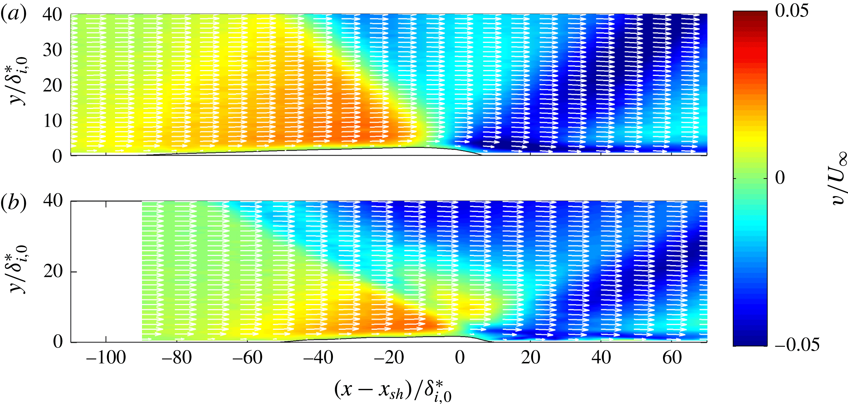
The mean wall-normal velocity component corresponding to figure 9.
The effect of the Mach number on the velocity field is illustrated in figures 11 and 12, for the smallest and largest Mach number tested in this study, $M=1.6$
and
$M=1.6$
and $M=2.3$
, respectively. Similar flow topologies are recorded for the low and high Mach number case, showing the typical features (separation bubble, compression/expansion waves) expected for a separated laminar SWBLI. One obvious difference is the smaller shock angle that occurs for the higher Mach number case. At
$M=2.3$
, respectively. Similar flow topologies are recorded for the low and high Mach number case, showing the typical features (separation bubble, compression/expansion waves) expected for a separated laminar SWBLI. One obvious difference is the smaller shock angle that occurs for the higher Mach number case. At $M=1.6$
the incident shock makes an angle of
$M=1.6$
the incident shock makes an angle of $39^{\circ }$
with the free stream, whereas for the
$39^{\circ }$
with the free stream, whereas for the $M=2.3$
case, this has been reduced to
$M=2.3$
case, this has been reduced to $28^{\circ }$
. These values compare well with those predicted by the oblique shock wave relations, which predict shock angles of
$28^{\circ }$
. These values compare well with those predicted by the oblique shock wave relations, which predict shock angles of $40^{\circ }$
and
$40^{\circ }$
and $27^{\circ }$
, respectively. Also the extent of the interaction has been reduced significantly for the higher Mach number case. The separation bubble for the
$27^{\circ }$
, respectively. Also the extent of the interaction has been reduced significantly for the higher Mach number case. The separation bubble for the $M=2.3$
case is approximately 35 % shorter than the bubble for the
$M=2.3$
case is approximately 35 % shorter than the bubble for the $M=1.6$
case.
$M=1.6$
case.
It may furthermore be noted that for the $M=2.3$
case there is a small region of upward flow velocity (positive
$M=2.3$
case there is a small region of upward flow velocity (positive $v$
) present around
$v$
) present around $(x-x_{sh})/\unicode[STIX]{x1D6FF}_{i,0}^{\ast }=3$
,
$(x-x_{sh})/\unicode[STIX]{x1D6FF}_{i,0}^{\ast }=3$
, $y/\unicode[STIX]{x1D6FF}_{i,0}^{\ast }=10$
), which is not existent for the
$y/\unicode[STIX]{x1D6FF}_{i,0}^{\ast }=10$
), which is not existent for the $M=1.6$
case. This feature is probably the result of aero-optical distortions present in the near vicinity of the shock wave. The camera configuration (viewing angles, aperture, etc.) was the same for both experiments, but the change in shock angle and Mach number can still lead to differences in the observed optical distortions. As highlighted in § 4.2, aero-optical distortions were typically observed to be slightly stronger for the higher Mach number case.
$M=1.6$
case. This feature is probably the result of aero-optical distortions present in the near vicinity of the shock wave. The camera configuration (viewing angles, aperture, etc.) was the same for both experiments, but the change in shock angle and Mach number can still lead to differences in the observed optical distortions. As highlighted in § 4.2, aero-optical distortions were typically observed to be slightly stronger for the higher Mach number case.
Finally, also the effect of the Reynolds number $Re_{x_{sh}}$
on the SWBLI was investigated. Figures 13 and 14 show the velocity field for shock impingement locations of
$Re_{x_{sh}}$
on the SWBLI was investigated. Figures 13 and 14 show the velocity field for shock impingement locations of $x_{sh}=41$
mm and
$x_{sh}=41$
mm and $x_{sh}=61$
mm, respectively, corresponding to
$x_{sh}=61$
mm, respectively, corresponding to $Re_{x_{sh}}=1.4\times 10^{6}$
and
$Re_{x_{sh}}=1.4\times 10^{6}$
and $2.1\times 10^{6}$
. The undisturbed boundary layer is fully laminar at
$2.1\times 10^{6}$
. The undisturbed boundary layer is fully laminar at $x_{sh}=41$
mm while an intermittency level of
$x_{sh}=41$
mm while an intermittency level of $\unicode[STIX]{x1D6FE}\sim 0.08$
is recorded at
$\unicode[STIX]{x1D6FE}\sim 0.08$
is recorded at $x=61$
mm. The boundary layers at the start of both interactions are still fully laminar in terms of their mean velocity profiles.
$x=61$
mm. The boundary layers at the start of both interactions are still fully laminar in terms of their mean velocity profiles.
The mean streamwise velocity component for two Mach numbers. The flow deflection angle and Reynolds number were fixed to $\unicode[STIX]{x1D703}=3^{\circ }$
and
$\unicode[STIX]{x1D703}=3^{\circ }$
and $Re_{x_{sh}}=1.8\times 10^{6}$
, respectively. (a)
$Re_{x_{sh}}=1.8\times 10^{6}$
, respectively. (a) $M=1.6$
and (b)
$M=1.6$
and (b) $M=2.3$
.
$M=2.3$
.
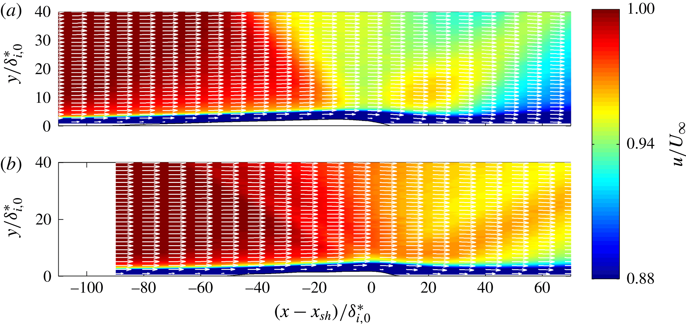
The mean wall-normal velocity component corresponding to figure 11.
Little differences are to be noted between the two test cases, except for the smaller separation bubble that occurs in the $x_{sh}=61$
mm case. The separation bubble measures approximately
$x_{sh}=61$
mm case. The separation bubble measures approximately $97\unicode[STIX]{x1D6FF}_{i,0}^{\ast }$
in length for the
$97\unicode[STIX]{x1D6FF}_{i,0}^{\ast }$
in length for the $x_{sh}=41$
mm case and
$x_{sh}=41$
mm case and $73\unicode[STIX]{x1D6FF}_{i,0}^{\ast }$
for the
$73\unicode[STIX]{x1D6FF}_{i,0}^{\ast }$
for the $x_{sh}=61$
mm case. This is attributed to the slightly transitional nature of the boundary layer at shock impingement, which makes it easier for the boundary layer to overcome the pressure rise at reattachment, consequently shrinking the separation bubble. The relation between transition and the size of the separation bubble is discussed in more detail in the following section.
$x_{sh}=61$
mm case. This is attributed to the slightly transitional nature of the boundary layer at shock impingement, which makes it easier for the boundary layer to overcome the pressure rise at reattachment, consequently shrinking the separation bubble. The relation between transition and the size of the separation bubble is discussed in more detail in the following section.
The mean streamwise velocity component for two Reynolds numbers. The flow deflection angle and Mach number were fixed to $\unicode[STIX]{x1D703}=3^{\circ }$
and
$\unicode[STIX]{x1D703}=3^{\circ }$
and $M=1.7$
, respectively. (a)
$M=1.7$
, respectively. (a) $Re_{x_{sh}}=1.4\times 10^{6}$
and (b)
$Re_{x_{sh}}=1.4\times 10^{6}$
and (b) $Re_{x_{sh}}=2.1\times 10^{6}$
.
$Re_{x_{sh}}=2.1\times 10^{6}$
.

The mean wall-normal velocity component corresponding to figure 13.
5.2 Relation between the separation bubble geometry and boundary layer transition
The goal of this section is to investigate the connection between the size and shape of the separation bubble and the state of the boundary layer throughout the interaction. This analysis is supported by the experimental data that were collected for a range of flow deflection angles, Mach numbers and Reynolds numbers. The height of the reversed flow region ( $u=0$
isoline) has been determined by applying a Falkner–Skan-based extrapolation procedure to the experimental data and the state of the boundary layer is estimated by calculating the incompressible shape factor over the separation bubble
$u=0$
isoline) has been determined by applying a Falkner–Skan-based extrapolation procedure to the experimental data and the state of the boundary layer is estimated by calculating the incompressible shape factor over the separation bubble $H_{i,aw}$
. Both data analysis techniques were discussed in § 3.3.
$H_{i,aw}$
. Both data analysis techniques were discussed in § 3.3.
Flow deflection angles were considered in the range of $\unicode[STIX]{x1D703}=1^{\circ }{-}5^{\circ }$
(
$\unicode[STIX]{x1D703}=1^{\circ }{-}5^{\circ }$
( $p_{3}/p_{1}=1.11{-}1.64$
). The corresponding extent of the reversed flow regions is presented in figure 15. The Mach and Reynolds number were fixed at
$p_{3}/p_{1}=1.11{-}1.64$
). The corresponding extent of the reversed flow regions is presented in figure 15. The Mach and Reynolds number were fixed at $M=1.7$
and
$M=1.7$
and $Re_{x_{sh}}=1.8\times 10^{6}$
(
$Re_{x_{sh}}=1.8\times 10^{6}$
( $x_{sh}=51$
mm), respectively. The length of the upstream portion of the reversed flow region is designated as
$x_{sh}=51$
mm), respectively. The length of the upstream portion of the reversed flow region is designated as $L_{u}$
and the downstream portion as
$L_{u}$
and the downstream portion as $L_{d}$
. These lengths are calculated by fitting straight lines to the experimental data points and calculating the intersection points with the wall (as illustrated in figure 15).
$L_{d}$
. These lengths are calculated by fitting straight lines to the experimental data points and calculating the intersection points with the wall (as illustrated in figure 15).
The reversed flow region as measured for a range of flow deflection angles ( $M=1.7$
,
$M=1.7$
, $x_{sh}=51$
mm).
$x_{sh}=51$
mm).

For shock waves stronger than $\unicode[STIX]{x1D703}>2^{\circ }$
(
$\unicode[STIX]{x1D703}>2^{\circ }$
( $p_{3}/p_{1}>1.22$
) it is observed that the downstream portion of the separation bubble keeps a near-constant length of
$p_{3}/p_{1}>1.22$
) it is observed that the downstream portion of the separation bubble keeps a near-constant length of $20\unicode[STIX]{x1D6FF}_{i,0}^{\ast }$
(see also figure 16). The upstream portion of the separation bubble
$20\unicode[STIX]{x1D6FF}_{i,0}^{\ast }$
(see also figure 16). The upstream portion of the separation bubble $L_{u}$
on the other hand shows a near-linear increase with the shock strength. For weak shock waves (
$L_{u}$
on the other hand shows a near-linear increase with the shock strength. For weak shock waves ( $\unicode[STIX]{x1D703}<2^{\circ }$
), however, a deviation from these trends is observed, as the upstream portion of the bubble is found to rapidly decrease in size with reducing flow deflection angles. The downstream portion of the bubble on the other hand increases in size when reducing the flow deflection angle. For flow deflection angles of
$\unicode[STIX]{x1D703}<2^{\circ }$
), however, a deviation from these trends is observed, as the upstream portion of the bubble is found to rapidly decrease in size with reducing flow deflection angles. The downstream portion of the bubble on the other hand increases in size when reducing the flow deflection angle. For flow deflection angles of $\unicode[STIX]{x1D703}=1^{\circ }{-}1.3^{\circ }$
(
$\unicode[STIX]{x1D703}=1^{\circ }{-}1.3^{\circ }$
( $p_{3}/p_{1}=1.11{-}1.14$
) a near-symmetrical
$p_{3}/p_{1}=1.11{-}1.14$
) a near-symmetrical $u=0$
isoline is recorded with
$u=0$
isoline is recorded with $L_{u}$
and
$L_{u}$
and $L_{d}$
being virtually the same.
$L_{d}$
being virtually the same.
The size of the reversed flow region as function of interaction strength ( $M=1.7$
,
$M=1.7$
, $x_{sh}=51$
mm).
$x_{sh}=51$
mm).
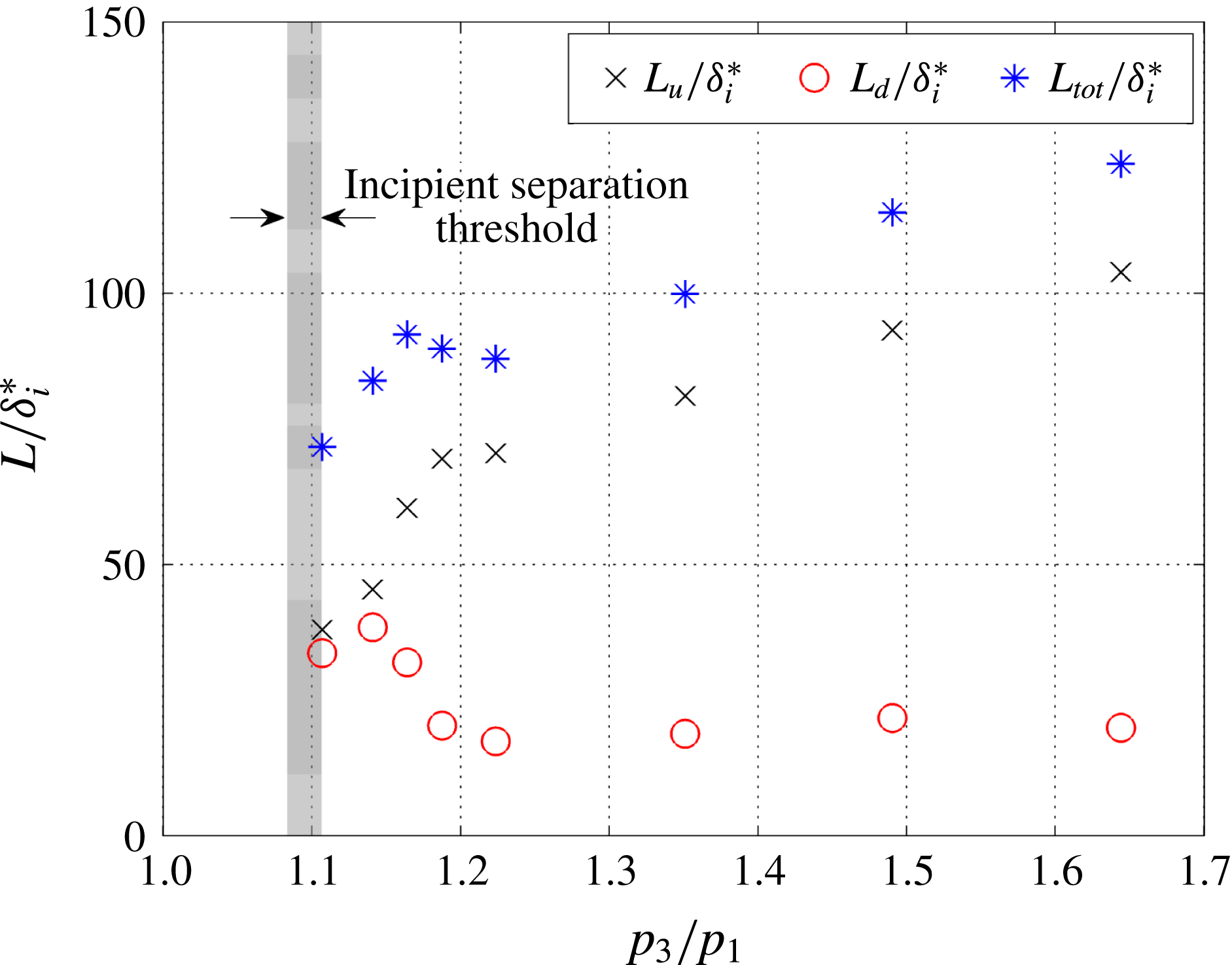
Shape factor development over the separation bubble for a range of flow deflection angles (a) and a comparison between natural and shock-induced transition (b) for $x_{sh}=51$
mm,
$x_{sh}=51$
mm, $M=1.7$
.
$M=1.7$
.
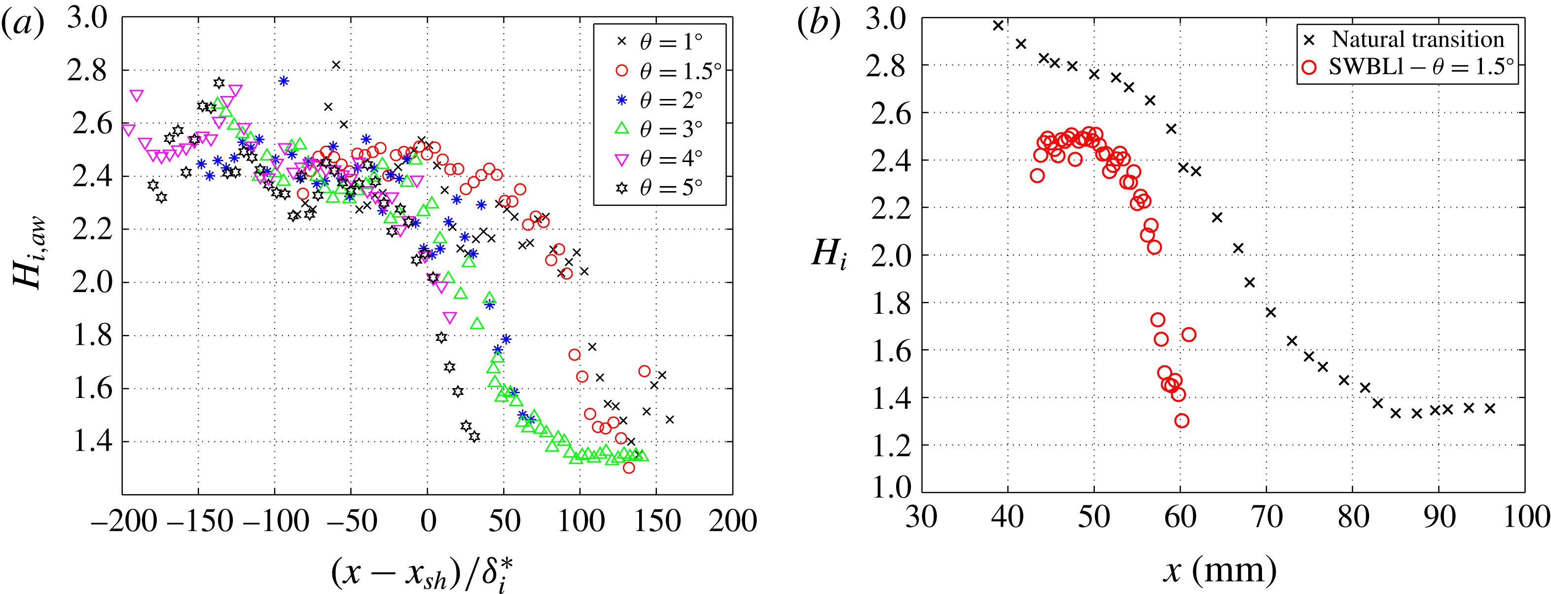
Effects of the Mach number on the reversed flow height (a) and the shape factor development throughout the interaction (b) for $x_{sh}=51$
mm,
$x_{sh}=51$
mm, $\unicode[STIX]{x1D703}=3^{\circ }$
.
$\unicode[STIX]{x1D703}=3^{\circ }$
.

The incipient separation threshold of figure 16 was computed from the free-interaction theory of Chapman et al. (Reference Chapman, Kuehn and Larson1957):
 $$\begin{eqnarray}\displaystyle p_{inc}/p_{1}=1+C_{sep}\unicode[STIX]{x1D6FE}M_{0}^{2}\sqrt{\frac{2C_{f_{0}}}{(M_{0}^{2}-1)^{0.5}}}. & & \displaystyle\end{eqnarray}$$
With $C_{f_{0}}$
and
$C_{f_{0}}$
and $M_{0}$
being the skin friction coefficient and the free stream Mach number at the interaction onset, respectively. The value of the constant
$M_{0}$
being the skin friction coefficient and the free stream Mach number at the interaction onset, respectively. The value of the constant $C_{sep}$
is obtained from experiments and difficult to determine accurately. Consequently various values are found in literature and the incipient separation threshold is presented as a band rather than a sharp line. The lower bound (
$C_{sep}$
is obtained from experiments and difficult to determine accurately. Consequently various values are found in literature and the incipient separation threshold is presented as a band rather than a sharp line. The lower bound ( $C_{sep}=0.79$
,
$C_{sep}=0.79$
, $p_{inc}/p_{1}=1.08$
) follows from the theoretical work of Rizzeta, Burggraf & Jenson (Reference Rizzeta, Burggraf and Jenson1978) while the upper bound (
$p_{inc}/p_{1}=1.08$
) follows from the theoretical work of Rizzeta, Burggraf & Jenson (Reference Rizzeta, Burggraf and Jenson1978) while the upper bound ( $C_{sep}=1$
,
$C_{sep}=1$
, $p_{inc}/p_{1}=1.11$
) corresponds to the results from Hakkinen et al. (Reference Hakkinen, Greber, Trilling and Abarbanel1959).
$p_{inc}/p_{1}=1.11$
) corresponds to the results from Hakkinen et al. (Reference Hakkinen, Greber, Trilling and Abarbanel1959).
For the $\unicode[STIX]{x1D703}=1^{\circ }$
case, which is close to the theoretical incipient separation boundary, still a relatively long separation bubble is recorded. A similar result was found in the experiments of Hakkinen et al. (Reference Hakkinen, Greber, Trilling and Abarbanel1959), who conjectured that for interactions close to incipient separation there will be a nonlinear growth of the separation bubble with shock strength.
$\unicode[STIX]{x1D703}=1^{\circ }$
case, which is close to the theoretical incipient separation boundary, still a relatively long separation bubble is recorded. A similar result was found in the experiments of Hakkinen et al. (Reference Hakkinen, Greber, Trilling and Abarbanel1959), who conjectured that for interactions close to incipient separation there will be a nonlinear growth of the separation bubble with shock strength.
The observed trends in figure 16 are strongly connected with the transition behaviour of the boundary layer, that is documented in figure 17(a). The metric $H_{i,aw}$
represents the incompressible shape factor of the boundary layer that is passing over the bubble. A shape factor of
$H_{i,aw}$
represents the incompressible shape factor of the boundary layer that is passing over the bubble. A shape factor of ${\sim}$
2.5 is typical for an attached flat-plate laminar boundary layer, whereas a value of
${\sim}$
2.5 is typical for an attached flat-plate laminar boundary layer, whereas a value of ${\sim}$
1.4 is typical for a turbulent boundary layer. Notwithstanding the measurement uncertainty affecting this parameter (see § 4.3), the transition location is clearly identifiable for all flow deflection angles. With increasing flow deflection angle, the transition front is found to move upstream, where transition is found to occur at the shock impingement location for the strongest shock wave (
${\sim}$
1.4 is typical for a turbulent boundary layer. Notwithstanding the measurement uncertainty affecting this parameter (see § 4.3), the transition location is clearly identifiable for all flow deflection angles. With increasing flow deflection angle, the transition front is found to move upstream, where transition is found to occur at the shock impingement location for the strongest shock wave ( $\unicode[STIX]{x1D703}=5^{\circ }$
) tested in this study. So, for all cases investigated, the boundary layer stays in an on average laminar state over the entire upstream part of the separation bubble.
$\unicode[STIX]{x1D703}=5^{\circ }$
) tested in this study. So, for all cases investigated, the boundary layer stays in an on average laminar state over the entire upstream part of the separation bubble.
Although the boundary layer is laminar in a mean flow sense, this does not imply that the boundary layer is free of instabilities while developing over the upstream part of the separation bubble. The recent works of Diop et al. (Reference Diop, Piponniau and Dupont2016), Larchevêque (Reference Larchevêque2016) showed clearly that boundary layer perturbations are amplified throughout the interaction. Especially the interaction onset and the shock impingement location were identified as regions where strong amplification occurs.
By reducing the shock strength, less amplification of these boundary layer perturbations is expected to occur, resulting in a delayed transition phase. This indeed also appears to be the case for the weaker shock waves tested in this study (see figure 17
a). A shape factor $H_{i,aw}$
of 2 is reached
$H_{i,aw}$
of 2 is reached ${\sim}100\unicode[STIX]{x1D6FF}_{i,0}^{\ast }$
downstream of the shock impingement location for the
${\sim}100\unicode[STIX]{x1D6FF}_{i,0}^{\ast }$
downstream of the shock impingement location for the $\unicode[STIX]{x1D703}=1^{\circ }$
and
$\unicode[STIX]{x1D703}=1^{\circ }$
and $1.5^{\circ }$
case, whereas for the
$1.5^{\circ }$
case, whereas for the $\unicode[STIX]{x1D703}=2^{\circ }$
case this value is reached already after
$\unicode[STIX]{x1D703}=2^{\circ }$
case this value is reached already after ${\sim}35\unicode[STIX]{x1D6FF}_{i,0}^{\ast }$
. This implies that for flow deflection angles in the range of
${\sim}35\unicode[STIX]{x1D6FF}_{i,0}^{\ast }$
. This implies that for flow deflection angles in the range of $1^{\circ }{-}1.5^{\circ }$
the boundary layer remains in a close to laminar state throughout the entire interaction. This also explains the longer downstream portion of the separation bubble, which has been observed for weak shock waves in figure 16. Stronger shocks promote boundary layer transition, which promotes reattachment, consequently shortening the downstream portion of the separation bubble.
$1^{\circ }{-}1.5^{\circ }$
the boundary layer remains in a close to laminar state throughout the entire interaction. This also explains the longer downstream portion of the separation bubble, which has been observed for weak shock waves in figure 16. Stronger shocks promote boundary layer transition, which promotes reattachment, consequently shortening the downstream portion of the separation bubble.
Even though transition sets in later for small flow deflection angles ( $\unicode[STIX]{x1D703}=1^{\circ }{-}1.5^{\circ }$
), the process is still strongly accelerated compared to that of natural transition (see figure 17
b). For the case of a weak impinging shock (
$\unicode[STIX]{x1D703}=1^{\circ }{-}1.5^{\circ }$
), the process is still strongly accelerated compared to that of natural transition (see figure 17
b). For the case of a weak impinging shock ( $\unicode[STIX]{x1D703}=1.5^{\circ }$
) transition takes place over a distance of 10 mm while for natural transition an extent of approximately 35 mm is observed. This reduction is likely related to the Kelvin–Helmholtz type of perturbations introduced in the shear layer of the downstream portion of the separation bubble (Sansica et al.
Reference Sansica, Sandham and Hu2014), which accelerates the subsequent process of transition.
$\unicode[STIX]{x1D703}=1.5^{\circ }$
) transition takes place over a distance of 10 mm while for natural transition an extent of approximately 35 mm is observed. This reduction is likely related to the Kelvin–Helmholtz type of perturbations introduced in the shear layer of the downstream portion of the separation bubble (Sansica et al.
Reference Sansica, Sandham and Hu2014), which accelerates the subsequent process of transition.
The effect of the Mach number on the interaction zone is presented in figure 18(a,b) for the reversed flow region and the incompressible shape factor, respectively. Mach numbers in the range of 1.6–2.3 were tested, for a fixed flow deflection angle and shock impingement location ( $\unicode[STIX]{x1D703}=3^{\circ }$
,
$\unicode[STIX]{x1D703}=3^{\circ }$
, $x_{sh}=51$
mm,
$x_{sh}=51$
mm, $Re_{x_{sh}}=1.8\times 10^{6}$
). It was already noted in § 5.1 that the topology of the interaction does not change substantially when changing the Mach number. The same is also observed when studying the
$Re_{x_{sh}}=1.8\times 10^{6}$
). It was already noted in § 5.1 that the topology of the interaction does not change substantially when changing the Mach number. The same is also observed when studying the $u=0$
isolines of figure 18(a). For all Mach numbers a flat, near-triangular reversed flow region is recorded, with a long upstream portion and a short downstream portion (i.e.
$u=0$
isolines of figure 18(a). For all Mach numbers a flat, near-triangular reversed flow region is recorded, with a long upstream portion and a short downstream portion (i.e. $L_{u}\gg L_{d}$
). The data for the
$L_{u}\gg L_{d}$
). The data for the $M=2.3$
are slightly noisier than that of the lower Mach number cases, due to increased near-wall seeding difficulties at the higher Mach numbers. The triangular shape can, however, still be recognized.
$M=2.3$
are slightly noisier than that of the lower Mach number cases, due to increased near-wall seeding difficulties at the higher Mach numbers. The triangular shape can, however, still be recognized.
Two trends with increasing Mach number can be observed in figure 18(a): (i) the length of the reversed flow region shrinks and (ii) the angle $\unicode[STIX]{x1D6FC}$
between the
$\unicode[STIX]{x1D6FC}$
between the $u=0$
isoline and the wall increases (see also table 7). The experimentally determined angles
$u=0$
isoline and the wall increases (see also table 7). The experimentally determined angles $\unicode[STIX]{x1D6FC}$
can be compared with the theoretical model for
$\unicode[STIX]{x1D6FC}$
can be compared with the theoretical model for $\unicode[STIX]{x1D6FC}$
by Hakkinen et al. (Reference Hakkinen, Greber, Trilling and Abarbanel1959). It should be remarked here that the experiments of Hakkinen et al. (Reference Hakkinen, Greber, Trilling and Abarbanel1959) were conducted for one Mach number only (
$\unicode[STIX]{x1D6FC}$
by Hakkinen et al. (Reference Hakkinen, Greber, Trilling and Abarbanel1959). It should be remarked here that the experiments of Hakkinen et al. (Reference Hakkinen, Greber, Trilling and Abarbanel1959) were conducted for one Mach number only ( $M=2$
). The Mach number dependency predicted by their theoretical model has therefore not been validated with experimental data. To the author’s knowledge this is the first study that compares the model of Hakkinen et al. with experimental data at a range of Mach numbers.
$M=2$
). The Mach number dependency predicted by their theoretical model has therefore not been validated with experimental data. To the author’s knowledge this is the first study that compares the model of Hakkinen et al. with experimental data at a range of Mach numbers.
Hakkinen et al. (Reference Hakkinen, Greber, Trilling and Abarbanel1959) used the principles of conservation of momentum to derive a relation between $\unicode[STIX]{x1D6FC}$
and the plateau pressure of the interaction
$\unicode[STIX]{x1D6FC}$
and the plateau pressure of the interaction $C_{p_{pl}}$
:
$C_{p_{pl}}$
:
 $$\begin{eqnarray}\displaystyle \unicode[STIX]{x1D6FC}=\text{atan}(0.5\unicode[STIX]{x1D6FD}C_{p_{pl}}). & & \displaystyle\end{eqnarray}$$
Here $\unicode[STIX]{x1D6FD}=\sqrt{M^{2}-1}$
and the plateau pressure of the interaction is related to the local skin friction coefficient by the following empirical relation:
$\unicode[STIX]{x1D6FD}=\sqrt{M^{2}-1}$
and the plateau pressure of the interaction is related to the local skin friction coefficient by the following empirical relation:
 $$\begin{eqnarray}\displaystyle C_{p_{pl}}=1.65\sqrt{\left(\frac{2C_{f_{0}}}{\unicode[STIX]{x1D6FD}}\right)}. & & \displaystyle\end{eqnarray}$$
The skin friction coefficient upstream of the interaction $C_{f_{0}}$
can be estimated from the Blasius boundary layer profile, with the Illingworth compressibility correction applied. Table 7 shows that the modelled and experimental values of
$C_{f_{0}}$
can be estimated from the Blasius boundary layer profile, with the Illingworth compressibility correction applied. Table 7 shows that the modelled and experimental values of $\unicode[STIX]{x1D6FC}$
are in good agreement with each other and typically deviate less than
$\unicode[STIX]{x1D6FC}$
are in good agreement with each other and typically deviate less than $0.1^{\circ }$
(
$0.1^{\circ }$
( ${\sim}$
5 % in a relative sense).
${\sim}$
5 % in a relative sense).
Parameters describing the reversed flow region for a range of Mach numbers.

The incompressible shape factor throughout the interaction is presented in figure 18(b). Within the Mach number range considered no clear differences are recorded in the transition behaviour. For all Mach numbers transition sets in directly downstream of the incident shock wave and a fully turbulent boundary layer is reached ${\sim}80\unicode[STIX]{x1D6FF}_{i,0}^{\ast }$
downstream of the shock.
${\sim}80\unicode[STIX]{x1D6FF}_{i,0}^{\ast }$
downstream of the shock.
Effects of the Reynolds number on the reversed flow height (a) and the shape factor development throughout the interaction (b) for $M=1.7$
,
$M=1.7$
, $\unicode[STIX]{x1D703}=3^{\circ }$
.
$\unicode[STIX]{x1D703}=3^{\circ }$
.

Correlation function $F$
for a range of flow deflection angles (a) and free stream Mach numbers (b).
$F$
for a range of flow deflection angles (a) and free stream Mach numbers (b).
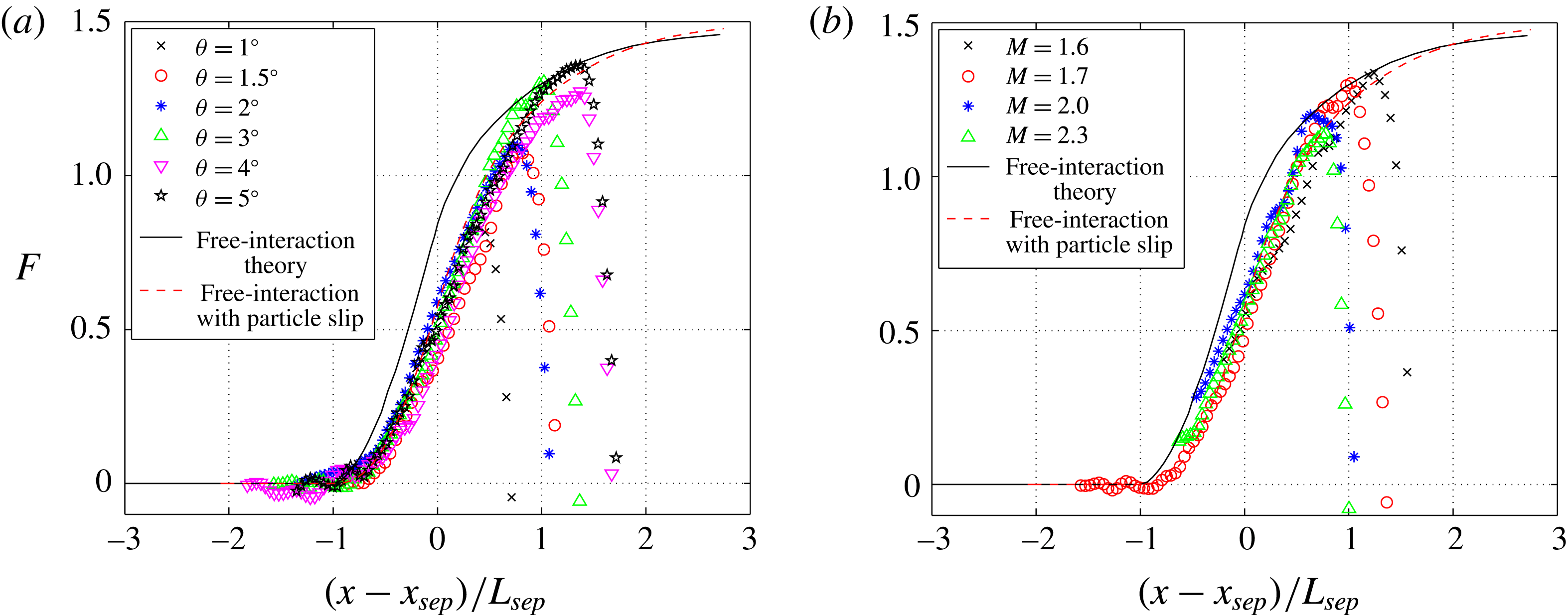
The effects of the Reynolds number on the reversed flow region are presented in figure 19(a). Shock impingement locations in the range of $x_{sh}=41{-}71$
mm are presented (
$x_{sh}=41{-}71$
mm are presented ( $Re_{x_{sh}}=1.4\times 10^{6}{-}2.5\times 10^{6}$
), where the data are normalized with the incompressible displacement thickness
$Re_{x_{sh}}=1.4\times 10^{6}{-}2.5\times 10^{6}$
), where the data are normalized with the incompressible displacement thickness $\unicode[STIX]{x1D6FF}_{i,0}^{\ast }$
measured at the onset of the respective interaction. For the
$\unicode[STIX]{x1D6FF}_{i,0}^{\ast }$
measured at the onset of the respective interaction. For the $x_{sh}=41$
and
$x_{sh}=41$
and $x_{sh}=51$
mm cases virtually the same reversed flow regions are recorded, with both the size and shape of the regions being in good agreement with each other. The reversed flow region for the
$x_{sh}=51$
mm cases virtually the same reversed flow regions are recorded, with both the size and shape of the regions being in good agreement with each other. The reversed flow region for the $x_{sh}=61$
mm case still shows the characteristic asymmetric triangular shape, but in terms of size it is significantly (37 %) smaller than the reversed flow regions recorded for the
$x_{sh}=61$
mm case still shows the characteristic asymmetric triangular shape, but in terms of size it is significantly (37 %) smaller than the reversed flow regions recorded for the $x_{sh}=41$
and 51 mm cases. This likely is due to the slightly transitional nature (
$x_{sh}=41$
and 51 mm cases. This likely is due to the slightly transitional nature ( $\unicode[STIX]{x1D6FE}\sim 0.08$
for the undisturbed boundary layer) for this case (see also the discussion in § 2.3). For the
$\unicode[STIX]{x1D6FE}\sim 0.08$
for the undisturbed boundary layer) for this case (see also the discussion in § 2.3). For the $x_{sh}=71$
mm case the boundary layer is clearly transitional (
$x_{sh}=71$
mm case the boundary layer is clearly transitional ( $\unicode[STIX]{x1D6FE}\sim 0.5$
) and a much smaller reversed flow region is recorded, which no longer has a triangular shape. PIV measurements were also performed for shock impingement locations of
$\unicode[STIX]{x1D6FE}\sim 0.5$
) and a much smaller reversed flow region is recorded, which no longer has a triangular shape. PIV measurements were also performed for shock impingement locations of $x_{sh}=81$
, 91 and 101 mm, but for these locations separation was no longer recorded.
$x_{sh}=81$
, 91 and 101 mm, but for these locations separation was no longer recorded.
The state of the boundary layer throughout the interaction is presented in figure 19(b) for the different shock impingement locations. Virtually the same development is observed for the $x_{sh}=41$
, 51 and 61 mm cases. The boundary layer remains in an on average laminar state up to the shock impingement location and after passing the shock wave quickly transitions into a turbulent state. The boundary layer for the
$x_{sh}=41$
, 51 and 61 mm cases. The boundary layer remains in an on average laminar state up to the shock impingement location and after passing the shock wave quickly transitions into a turbulent state. The boundary layer for the $x_{sh}=61$
mm case appears to transition slightly earlier than the boundary layer for the
$x_{sh}=61$
mm case appears to transition slightly earlier than the boundary layer for the $x_{sh}=41$
and 51 mm cases. This is probably the result of the already slightly transitional nature of the boundary layer at the moment of crossing the shock wave.
$x_{sh}=41$
and 51 mm cases. This is probably the result of the already slightly transitional nature of the boundary layer at the moment of crossing the shock wave.
For the transitional interaction ( $x_{sh}=71$
mm), it can be noticed that the boundary layer shows a strong development over the separation bubble. Starting from a nearly laminar boundary layer, it develops into a turbulent profile before the point of reattachment. Towards reattachment, the boundary layer profile temporarily becomes slightly less full (probably caused by the strong pressure rise at reattachment), but a quick recovery is observed, and within
$x_{sh}=71$
mm), it can be noticed that the boundary layer shows a strong development over the separation bubble. Starting from a nearly laminar boundary layer, it develops into a turbulent profile before the point of reattachment. Towards reattachment, the boundary layer profile temporarily becomes slightly less full (probably caused by the strong pressure rise at reattachment), but a quick recovery is observed, and within ${\sim}60\unicode[STIX]{x1D6FF}_{i,0}^{\ast }$
a shape factor of 1.4 is reached, typical for an equilibrium turbulent boundary layer.
${\sim}60\unicode[STIX]{x1D6FF}_{i,0}^{\ast }$
a shape factor of 1.4 is reached, typical for an equilibrium turbulent boundary layer.
5.3 Free interactions
The specific goal of this section is to investigate whether the flow field at the onset of the interaction adheres to the principles of the free-interaction theory (Chapman et al.
Reference Chapman, Kuehn and Larson1957). The free-interaction theory states that the scaling of the first part of the interaction should only depend upon upstream flow properties and not on the downstream flow conditions. The initial pressure rise through the interaction should therefore, in principle, be independent of the shock strength and the type of interaction (e.g. oblique shock wave reflections or compression corner). From the free-interaction theory it follows that the wall pressure coefficient $C_{p}$
through the first part of the interaction can be described by:
$C_{p}$
through the first part of the interaction can be described by:
 $$\begin{eqnarray}\displaystyle C_{p}(\bar{x})=F(\bar{x})\sqrt{\frac{2C_{f_{0}}}{(M_{0}^{2}-1)^{0.5}}}, & & \displaystyle\end{eqnarray}$$
where $\bar{x}$
is defined as
$\bar{x}$
is defined as $\bar{x}=(x-x_{sep})/L_{sep}$
. In this formulation
$\bar{x}=(x-x_{sep})/L_{sep}$
. In this formulation $x_{sep}$
defines the separation location and
$x_{sep}$
defines the separation location and $L_{sep}$
defines the distance between the interaction onset location (where the pressure rise first occurs) and the separation location. According to this theory,
$L_{sep}$
defines the distance between the interaction onset location (where the pressure rise first occurs) and the separation location. According to this theory, $F(\bar{x})$
in (5.4) is a universal correlation function, which couples the pressure rise through the interaction to the upstream flow conditions. The correlation function
$F(\bar{x})$
in (5.4) is a universal correlation function, which couples the pressure rise through the interaction to the upstream flow conditions. The correlation function $F$
for laminar interactions that is used in this study has been obtained from the work of Erdos & Pallone (Reference Erdos and Pallone1963) and is plotted as the black solid line in figure 20(a,b). At the separation point
$F$
for laminar interactions that is used in this study has been obtained from the work of Erdos & Pallone (Reference Erdos and Pallone1963) and is plotted as the black solid line in figure 20(a,b). At the separation point $F$
equals 0.81 and at the pressure plateau
$F$
equals 0.81 and at the pressure plateau $F$
approximately reaches a value of 1.47.
$F$
approximately reaches a value of 1.47.
The free-interaction theory is well established for low and moderate Reynolds number flows ( $Re_{\unicode[STIX]{x1D6FF}_{99}}<10^{5}$
), with relatively strong shock waves (Delery & Marvin Reference Delery and Marvin1986). Plenty of data are available which confirm the universal nature of the correlation function
$Re_{\unicode[STIX]{x1D6FF}_{99}}<10^{5}$
), with relatively strong shock waves (Delery & Marvin Reference Delery and Marvin1986). Plenty of data are available which confirm the universal nature of the correlation function $F$
and the validity of (5.4). For weak laminar interactions, on the other hand, much less information is available. In this context, a weak interaction is defined as an interaction where the pressure plateau is not reached. This section provides new evidence that the free-interaction concept also holds true for weak shock waves and even for incipiently separated laminar interactions.
$F$
and the validity of (5.4). For weak laminar interactions, on the other hand, much less information is available. In this context, a weak interaction is defined as an interaction where the pressure plateau is not reached. This section provides new evidence that the free-interaction concept also holds true for weak shock waves and even for incipiently separated laminar interactions.
Notwithstanding that no detailed surface pressure data were recorded in the present study, the function $F$
can also be extracted from the PIV velocity data. Supersonic linear theory is used to convert the velocity field upstream of the impinging shock wave to a pressure field. Linear theory is applicable here because of the relatively small flow deflection angles
$F$
can also be extracted from the PIV velocity data. Supersonic linear theory is used to convert the velocity field upstream of the impinging shock wave to a pressure field. Linear theory is applicable here because of the relatively small flow deflection angles $\unicode[STIX]{x1D703}_{flow}$
, which never exceed
$\unicode[STIX]{x1D703}_{flow}$
, which never exceed $2^{\circ }$
, allowing the pressure coefficient to be calculated as:
$2^{\circ }$
, allowing the pressure coefficient to be calculated as:
 $$\begin{eqnarray}\displaystyle C_{p}=\frac{2\unicode[STIX]{x1D703}_{flow}}{\sqrt{M^{2}-1}}. & & \displaystyle\end{eqnarray}$$
The flow deflection angles are calculated at multiple $y$
-locations (in the range of
$y$
-locations (in the range of $y/\unicode[STIX]{x1D6FF}_{i,0}^{\ast }=5{-}10$
) to improve the accuracy of the velocity to pressure conversion. The measured flow deflection angles were projected back onto the wall along the Mach angle, to account for the horizontal shift in the profiles. The deflection angles were then averaged and converted to a
$y/\unicode[STIX]{x1D6FF}_{i,0}^{\ast }=5{-}10$
) to improve the accuracy of the velocity to pressure conversion. The measured flow deflection angles were projected back onto the wall along the Mach angle, to account for the horizontal shift in the profiles. The deflection angles were then averaged and converted to a $C_{p}$
distribution using (5.5). The values for
$C_{p}$
distribution using (5.5). The values for $F$
as function of
$F$
as function of $(x-x_{sep})/L$
were obtained by applying (5.4) to the experimental
$(x-x_{sep})/L$
were obtained by applying (5.4) to the experimental $C_{p}$
distributions.
$C_{p}$
distributions.
Figure 20(a) compares the experimentally obtained correlation functions $F$
for the different flow deflection angles, compared with the function
$F$
for the different flow deflection angles, compared with the function $F$
described by Erdos & Pallone (Reference Erdos and Pallone1963). The experimental data for the different interactions are in good agreement: from the weakest interaction (
$F$
described by Erdos & Pallone (Reference Erdos and Pallone1963). The experimental data for the different interactions are in good agreement: from the weakest interaction ( $\unicode[STIX]{x1D703}=1^{\circ }$
) up to the strongest interaction (
$\unicode[STIX]{x1D703}=1^{\circ }$
) up to the strongest interaction ( $\unicode[STIX]{x1D703}=5^{\circ }$
) tested in this study, all experiments show virtually the same distribution of
$\unicode[STIX]{x1D703}=5^{\circ }$
) tested in this study, all experiments show virtually the same distribution of $F$
. This pressure rise, however, appears to be slightly delayed with respect to the curve of Erdos & Pallone (Reference Erdos and Pallone1963). This is attributed to the effect of particle slip, which is inherent to any particle-based experiment performed in supersonic flow (see § 4.1). To assess if this effect can indeed account for the observed discrepancy, the function
$F$
. This pressure rise, however, appears to be slightly delayed with respect to the curve of Erdos & Pallone (Reference Erdos and Pallone1963). This is attributed to the effect of particle slip, which is inherent to any particle-based experiment performed in supersonic flow (see § 4.1). To assess if this effect can indeed account for the observed discrepancy, the function $F$
of Erdos & Pallone (Reference Erdos and Pallone1963) was also subjected to the effects of particle slip. This was achieved by converting it to a velocity field upon which a simple particle slip model (Melling Reference Melling1997) is used to get an equivalent ‘PIV-filtered’ velocity field. The only input to this model is the particle response time, which for the
$F$
of Erdos & Pallone (Reference Erdos and Pallone1963) was also subjected to the effects of particle slip. This was achieved by converting it to a velocity field upon which a simple particle slip model (Melling Reference Melling1997) is used to get an equivalent ‘PIV-filtered’ velocity field. The only input to this model is the particle response time, which for the $\text{TiO}_{2}$
particles was determined to be
$\text{TiO}_{2}$
particles was determined to be $\unicode[STIX]{x1D70F}_{p}=2.5~\unicode[STIX]{x03BC}\text{s}$
. The filtered velocity field is again converted back to a pressure field using linear supersonic theory, yielding a ‘PIV-filtered’ version of the function
$\unicode[STIX]{x1D70F}_{p}=2.5~\unicode[STIX]{x03BC}\text{s}$
. The filtered velocity field is again converted back to a pressure field using linear supersonic theory, yielding a ‘PIV-filtered’ version of the function $F$
. This filtered version of
$F$
. This filtered version of $F$
appears to be in excellent agreement with the experimental data acquired during this study.
$F$
appears to be in excellent agreement with the experimental data acquired during this study.
Figure 20(b) shows a similar comparison for the effects of the Mach number of the function $F$
. Again all the data collapse onto one curve. Figure 20(a,b) therefore provides strong experimental evidence that the free-interaction theory also holds for weak laminar interactions, where the pressure plateau is not established.
$F$
. Again all the data collapse onto one curve. Figure 20(a,b) therefore provides strong experimental evidence that the free-interaction theory also holds for weak laminar interactions, where the pressure plateau is not established.
6 Conclusions
A parametric study has been conducted into laminar and transitional oblique shock wave reflections, by variation of the Mach number, Reynolds number and shock strength. The Mach number was varied from $M_{\infty }=1.6$
to 2.3, the Reynolds number from
$M_{\infty }=1.6$
to 2.3, the Reynolds number from $Re_{x_{sh}}=1.4\times 10^{6}$
to
$Re_{x_{sh}}=1.4\times 10^{6}$
to $3.5\times 10^{6}$
and the flow deflection angle from
$3.5\times 10^{6}$
and the flow deflection angle from $\unicode[STIX]{x1D703}=1^{\circ }$
to
$\unicode[STIX]{x1D703}=1^{\circ }$
to $5^{\circ }$
(
$5^{\circ }$
( $p_{3}/p_{1}=1.11$
to 1.64). All measurements were performed on a full-span flat-plate model, with the oblique shock wave being generated by a partial-span shock generator. High-resolution particle image velocimetry (PIV) measurements were performed for all test cases, delivering mean velocity field data in the interaction region.
$p_{3}/p_{1}=1.11$
to 1.64). All measurements were performed on a full-span flat-plate model, with the oblique shock wave being generated by a partial-span shock generator. High-resolution particle image velocimetry (PIV) measurements were performed for all test cases, delivering mean velocity field data in the interaction region.
The PIV measurements reveal a long, flat and triangular reversed flow region for the laminar interactions. For relatively strong shock waves ( $\unicode[STIX]{x1D703}>2^{\circ }$
,
$\unicode[STIX]{x1D703}>2^{\circ }$
, $p_{3}/p_{1}>1.22$
) it is found that the horizontal distance
$p_{3}/p_{1}>1.22$
) it is found that the horizontal distance $L_{u}$
between the point of boundary layer separation and the top of the bubble increases linearly with shock strength, whereas the horizontal distance
$L_{u}$
between the point of boundary layer separation and the top of the bubble increases linearly with shock strength, whereas the horizontal distance $L_{d}$
between the top of the separation bubble and reattachment remains virtually constant (
$L_{d}$
between the top of the separation bubble and reattachment remains virtually constant ( $L_{d}\sim 20\unicode[STIX]{x1D6FF}_{i,0}^{\ast }$
) with shock strength. The boundary layer remains in an on average laminar state over the upstream part of the bubble, but transitions rapidly after passing the incident shock wave.
$L_{d}\sim 20\unicode[STIX]{x1D6FF}_{i,0}^{\ast }$
) with shock strength. The boundary layer remains in an on average laminar state over the upstream part of the bubble, but transitions rapidly after passing the incident shock wave.
On the other hand, for relatively weak shock waves the boundary layer is capable of maintaining its laminarity longer and transition sets in approximately ${\sim}100\unicode[STIX]{x1D6FF}_{i,0}^{\ast }$
downstream of the incident shock wave. As a result of the reduced mixing in the shear layer, reattachment is delayed with a corresponding increase in the downstream length of the separation bubble
${\sim}100\unicode[STIX]{x1D6FF}_{i,0}^{\ast }$
downstream of the incident shock wave. As a result of the reduced mixing in the shear layer, reattachment is delayed with a corresponding increase in the downstream length of the separation bubble $L_{d}$
, from approximately
$L_{d}$
, from approximately $20\unicode[STIX]{x1D6FF}_{i,0}^{\ast }$
to
$20\unicode[STIX]{x1D6FF}_{i,0}^{\ast }$
to $38\unicode[STIX]{x1D6FF}_{i,0}^{\ast }$
when reducing the flow deflection angle from
$38\unicode[STIX]{x1D6FF}_{i,0}^{\ast }$
when reducing the flow deflection angle from $\unicode[STIX]{x1D703}=2^{\circ }$
to
$\unicode[STIX]{x1D703}=2^{\circ }$
to $1.3^{\circ }$
, respectively. This clearly shows the strong connection between boundary layer transition, separation bubble size and flow deflection angle. Even though transition sets in later for weak shock waves (
$1.3^{\circ }$
, respectively. This clearly shows the strong connection between boundary layer transition, separation bubble size and flow deflection angle. Even though transition sets in later for weak shock waves ( $\unicode[STIX]{x1D703}=1^{\circ }{-}1.5^{\circ }$
), the process of transition is still strongly accelerated compared to that of natural transition. Natural transition takes place over the extent of approximately 35 mm, whereas with the presence of an impinging shock wave (
$\unicode[STIX]{x1D703}=1^{\circ }{-}1.5^{\circ }$
), the process of transition is still strongly accelerated compared to that of natural transition. Natural transition takes place over the extent of approximately 35 mm, whereas with the presence of an impinging shock wave ( $\unicode[STIX]{x1D703}=1.5^{\circ }$
) this has been reduced to approximately 10 mm.
$\unicode[STIX]{x1D703}=1.5^{\circ }$
) this has been reduced to approximately 10 mm.
Increasing the Mach number while keeping the Reynolds number and flow deflection angle constant ( $Re_{x_{sh}}=1.8\times 10^{6}$
,
$Re_{x_{sh}}=1.8\times 10^{6}$
, $\unicode[STIX]{x1D703}=3^{\circ }$
) leads to a monotonic decrease in the size of the reversed flow region. On the other hand, the angle
$\unicode[STIX]{x1D703}=3^{\circ }$
) leads to a monotonic decrease in the size of the reversed flow region. On the other hand, the angle $\unicode[STIX]{x1D6FC}$
between the
$\unicode[STIX]{x1D6FC}$
between the $u=0$
isoline and the wall is found to monotonically increase with Mach number, from
$u=0$
isoline and the wall is found to monotonically increase with Mach number, from $1.7^{\circ }$
to
$1.7^{\circ }$
to $2.2^{\circ }$
for
$2.2^{\circ }$
for $M=1.6$
to 2.3, respectively. These values are in good agreement with the predictions from the empirical scaling model of Hakkinen et al. (Reference Hakkinen, Greber, Trilling and Abarbanel1959) for laminar oblique shock wave reflections.
$M=1.6$
to 2.3, respectively. These values are in good agreement with the predictions from the empirical scaling model of Hakkinen et al. (Reference Hakkinen, Greber, Trilling and Abarbanel1959) for laminar oblique shock wave reflections.
The shock location Reynolds number $Re_{x_{sh}}$
was varied from
$Re_{x_{sh}}$
was varied from $1.4\times 10^{6}$
to
$1.4\times 10^{6}$
to $3.5\times 10^{6}$
(
$3.5\times 10^{6}$
( $x_{sh}=41$
to 101 mm). A previous boundary layer study (Giepman et al.
Reference Giepman, Schrijer and Van Oudheusden2015) revealed that the boundary layer is laminar for
$x_{sh}=41$
to 101 mm). A previous boundary layer study (Giepman et al.
Reference Giepman, Schrijer and Van Oudheusden2015) revealed that the boundary layer is laminar for $Re_{x_{sh}}=1.4\times 10^{6}$
and
$Re_{x_{sh}}=1.4\times 10^{6}$
and $1.8\times 10^{6}$
, transitional for
$1.8\times 10^{6}$
, transitional for $Re_{x_{sh}}=2.1\times 10^{6}$
to
$Re_{x_{sh}}=2.1\times 10^{6}$
to $3.2\times 10^{6}$
mm and fully turbulent for
$3.2\times 10^{6}$
mm and fully turbulent for $Re_{x_{sh}}=3.5\times 10^{6}$
. Separation is only recorded for
$Re_{x_{sh}}=3.5\times 10^{6}$
. Separation is only recorded for $Re_{x_{sh}}=1.4\times 10^{6}$
to
$Re_{x_{sh}}=1.4\times 10^{6}$
to $2.5\times 10^{6}$
(
$2.5\times 10^{6}$
( $\unicode[STIX]{x1D6FE}=0{-}0.5$
), with the largest bubble recorded for the laminar cases. The two laminar cases deliver virtually the same size/shape of separation bubble and also the recorded transition process appears to be very similar. This indicates that the interaction is relatively insensitive to changes in the Reynolds number, as long as the incoming boundary layer is fully laminar. The size of the bubble is reduced significantly when the boundary layer is (slightly) transitional. Although the intermittency level for
$\unicode[STIX]{x1D6FE}=0{-}0.5$
), with the largest bubble recorded for the laminar cases. The two laminar cases deliver virtually the same size/shape of separation bubble and also the recorded transition process appears to be very similar. This indicates that the interaction is relatively insensitive to changes in the Reynolds number, as long as the incoming boundary layer is fully laminar. The size of the bubble is reduced significantly when the boundary layer is (slightly) transitional. Although the intermittency level for $Re_{x_{sh}}=2.1\times 10^{6}$
equals only
$Re_{x_{sh}}=2.1\times 10^{6}$
equals only $\unicode[STIX]{x1D6FE}=0.08$
, the recorded bubble size nevertheless is 24 % smaller than the bubble size recorded for the
$\unicode[STIX]{x1D6FE}=0.08$
, the recorded bubble size nevertheless is 24 % smaller than the bubble size recorded for the $Re_{x_{sh}}=1.8\times 10^{6}$
case, for which the boundary layer is still fully laminar.
$Re_{x_{sh}}=1.8\times 10^{6}$
case, for which the boundary layer is still fully laminar.
The flow deflection angles upstream of the incident shock wave are relatively small ( $\unicode[STIX]{x1D703}_{flow}<2^{\circ }$
) and justify the use of linear supersonic theory to convert the measured velocities to wall pressures. The calculated pressure distributions compare favourably with the free-interaction theory of Chapman et al. (Reference Chapman, Kuehn and Larson1957) after a correction was applied for the effects of particle slip. Although the free-interaction theory is well established for relatively strong shock waves (Delery & Marvin Reference Delery and Marvin1986), much less information is available in literature for weak interactions, where a pressure plateau is never reached. The data of this study provide convincing evidence that the free-interaction concept also holds for incipiently separated oblique shock wave reflections with a laminar incoming boundary layer.
$\unicode[STIX]{x1D703}_{flow}<2^{\circ }$
) and justify the use of linear supersonic theory to convert the measured velocities to wall pressures. The calculated pressure distributions compare favourably with the free-interaction theory of Chapman et al. (Reference Chapman, Kuehn and Larson1957) after a correction was applied for the effects of particle slip. Although the free-interaction theory is well established for relatively strong shock waves (Delery & Marvin Reference Delery and Marvin1986), much less information is available in literature for weak interactions, where a pressure plateau is never reached. The data of this study provide convincing evidence that the free-interaction concept also holds for incipiently separated oblique shock wave reflections with a laminar incoming boundary layer.
Acknowledgements
This work has been supported by the European FP7 project TFAST (Grant Agreement No. 265455), which studies the effects of boundary layer transition on SWBLIs. The authors also gratefully acknowledge the other TFAST partners for their shared insights and knowledge.


 Open access