


1. Introduction
The solar corona and the solar wind exhibit temperature and velocity profiles that cannot be fully explained by Parker’s (Reference Parker1958) simple isothermal hydrodynamic model. The mechanisms that supply the energy required to explain the differences remain debated (De Moortel & Browning Reference De Moortel and Browning2015; Cranmer, Gibson & Riley Reference Cranmer, Gibson and Riley2017; Chandran Reference Chandran2021). A prominent idea is that motions in the photosphere launch Alfvénic waves into open flux tubes. These waves travel outward and somehow dissipate, heating the plasma (De Pontieu et al. Reference De Pontieu2007; Cranmer Reference Cranmer2009), both raising plasma temperature and increasing magnetic or wave pressure, thereby contributing to wind acceleration (Tu Reference Tu1987; Cranmer et al. Reference Cranmer, van Ballegooijen, Adriaan and Edgar2007). Observational support comes from measurements of ubiquitous Alfvénic fluctuations in fast solar-wind streams, as reported by early spacecraft (Belcher & Davis Reference Belcher and Davis1971; Tu & Marsch Reference Tu and Marsch1995) and consolidated in later reviews (Bruno & Carbone Reference Bruno and Carbone2013). Recent in situ data indicate that large-amplitude Alfvén waves can carry substantial energy for coronal heating and wind acceleration (Halekas et al. Reference Raouafi2023; Rivera et al. Reference Rivera2024).
However, a fundamental theoretical limitation arises because, in a homogeneous medium, Alfvén waves propagating in a single direction do not interact nonlinearly and thus cannot by themselves sustain a turbulent cascade that dissipate their energy (Kraichnan Reference Kraichnan1965; Barnes & Hollweg Reference Barnes and Hollweg1974). In the solar wind, counter-propagating fluctuations can be generated by partial reflection of outward waves from background Alfvén-speed gradients, a process termed ‘reflection-driven turbulence’ (RDT) (Velli, Grappin & Mangeney Reference Velli, Grappin and Mangeney1989; Velli Reference Velli1993; Matthaeus et al. Reference Matthaeus, Zank, Oughton, Mullan and Dmitruk1999; Verdini & Velli Reference Verdini and Velli2007). Numerical and analytical models suggest this mechanism can supply a significant fraction of the heating necessary to maintain fast solar-wind streams (Chandran & Hollweg Reference Chandran and Hollweg2009; Verdini, Velli & Buchlin Reference Verdini, Velli and Buchlin2009; Chandran & Perez Reference Chandran and Perez2019; Chandran Reference Chandran2021). We note that, when compressibility is included, parametric decay instability can also generate counter-propagating and compressible fluctuations from finite-amplitude Alfvén waves, although the relative importance of this mechanism in solar-wind turbulence evolution remains debated (Malara, Primavera & Veltri Reference Malara, Primavera and Veltri2000).
Most models of solar-wind turbulence, and RDT specifically, assume a purely radial-background magnetic field for simplicity. Beyond the Alfvén point, where the solar-wind speed equals the Alfvén speed, the Sun’s rotation twists the field into the well-known Parker spiral (PS) (Parker Reference Parker1958; Weber & Davis Reference Weber and Davis1967). Close to the Sun, the spiral angle is very small, but beyond approximately $0.3$
–
$0.3$
– $1$
AU the azimuthal component becomes significant, such that it could alter wave propagation and nonlinear coupling (Verdini, Velli & Buchlin Reference Verdini, Velli and Buchlin2008; Owens & Forsyth Reference Owens and Forsyth2013; Verdini et al. Reference Verdini, Grappin, Alexandrova and Lion2018).
$1$
AU the azimuthal component becomes significant, such that it could alter wave propagation and nonlinear coupling (Verdini, Velli & Buchlin Reference Verdini, Velli and Buchlin2008; Owens & Forsyth Reference Owens and Forsyth2013; Verdini et al. Reference Verdini, Grappin, Alexandrova and Lion2018).
The goal of this paper is to quantify how PS geometry modifies RDT and the heating it causes in the super-Alfvénic solar wind. We argue that the relevant change to the standard Dmitruk et al. (Reference Dmitruk, Matthaeus, Milano, Oughton, Zank and Mullan2002) phenomenology of RDT due to the PS is that the evolution of the characteristic scales of the turbulence in the perpendicular and parallel directions are modified by the mean field’s direction. We then study this phenomenology using the expanding-box model (EBM) (Grappin, Velli & Mangeney Reference Grappin, Velli and Mangeney1993) to follow a small plasma parcel advected outward, presenting a suite of three-dimensional compressible magnetohydrodynamic (MHD) simulations initialised with strongly outward-dominated $\boldsymbol{z}^+$
fluctuations. We find that the RDT picture remains broadly valid in PS geometry – the same reflection-driven dynamics operates, but the controlling scales change. Perpendicular expansion stretches eddies into pancake-like structures, while the growing azimuthal field in the PS rotates the mean field relative to those pancakes and therefore ‘cuts across’ them; this geometric change produces smaller effective perpendicular scales than in the radial case. As a result the two transverse correlation lengths evolve differently and the effective perpendicular outer scale in a PS background tends to saturate rather than grow indefinitely. This causes the expansion-to-nonlinearity ratio, termed
$\boldsymbol{z}^+$
fluctuations. We find that the RDT picture remains broadly valid in PS geometry – the same reflection-driven dynamics operates, but the controlling scales change. Perpendicular expansion stretches eddies into pancake-like structures, while the growing azimuthal field in the PS rotates the mean field relative to those pancakes and therefore ‘cuts across’ them; this geometric change produces smaller effective perpendicular scales than in the radial case. As a result the two transverse correlation lengths evolve differently and the effective perpendicular outer scale in a PS background tends to saturate rather than grow indefinitely. This causes the expansion-to-nonlinearity ratio, termed $\chi _{\textrm {exp}}$
, to decrease less rapidly and the system remains in a sustained, imbalanced nonlinear state. By contrast, in radial geometry the perpendicular scale grows with expansion,
$\chi _{\textrm {exp}}$
, to decrease less rapidly and the system remains in a sustained, imbalanced nonlinear state. By contrast, in radial geometry the perpendicular scale grows with expansion, $\chi _{\textrm {exp}}$
falls, and the cascade can shut off, leaving a magnetically dominated state with little associated heating.
$\chi _{\textrm {exp}}$
falls, and the cascade can shut off, leaving a magnetically dominated state with little associated heating.
The paper is organised as follows. In § 2 we develop the theoretical framework for turbulence evolution and introduce the compressible expanding-box MHD model employed in our study. We extend the simple reflection-driven phenomenology of Dmitruk et al. (Reference Dmitruk, Matthaeus, Milano, Oughton, Zank and Mullan2002) and show how PS geometry alters reflection, projected perpendicular scales, and the resulting nonlinear time scales. In § 3 we summarise the numerical method, list key parameters and resolution choices and specify the initial conditions used in the simulation suite. In § 4, we test the theoretical expectations of § 2 by examining evolution of outward/inward energies, normalised cross-helicity and the competing nonlinear and expansion time scales demonstrating how these diagnostics depend on the PS, in general agreement with the phenomenology. Section 5 explores various other diagnostics for the purpose of comparing with observations, reporting the parametric evolution of cross-helicity and residual energy, switchback statistics, magnetic compressibility and synthetic fly-by traces for comparison with spacecraft measurements. Finally, § 6 summarises the main results and discusses their implications for existing theory and in situ observations.
2. Theoretical framework
In this section, we build a theoretical model to describe how solar-wind expansion and large-scale magnetic-field geometry shape Alfvénic turbulence. We introduce the expanding-box formalism to capture the kinematic effects of transverse expansion on fields and their length scales (Grappin et al. Reference Grappin, Velli and Mangeney1993), and formulate the dynamics in terms of Elsässer variables to make the reflection-driven coupling explicit. Building on this foundation, we outline RDT and derive the Dmitruk et al. (Reference Dmitruk, Matthaeus, Milano, Oughton, Zank and Mullan2002) decay phenomenology, extending this to include the PS. This framework both motivates the simulations and diagnostics developed later and provides testable predictions for our simulations.
2.1. Governing equations for reflection-driven turbulence
The solar wind’s turbulent evolution is governed by the interplay between reflection and nonlinear interactions. To model this in regions beyond the Alfvén critical point, where the flow becomes super-Alfvénic, we adopt the EBM (Grappin et al. Reference Grappin, Velli and Mangeney1993), which approximates the spherical expansion of the solar wind in a Cartesian patch of wind co-moving with the constant radial flow velocity $ U$
. Aligning the
$ U$
. Aligning the $ x$
-axis with the radial direction, the EBM introduces an expansion factor
$ x$
-axis with the radial direction, the EBM introduces an expansion factor $ a(t) = R(t)/R_0$
, where
$ a(t) = R(t)/R_0$
, where $ R(t) = R_0 + U t$
is the heliocentric distance for some initial
$ R(t) = R_0 + U t$
is the heliocentric distance for some initial $R_0$
, and modifies spatial gradients as
$R_0$
, and modifies spatial gradients as $ \tilde {\boldsymbol{\nabla }} = (\partial _x, a^{-1}\partial _y, a^{-1}\partial _z)$
, viz.,
$ \tilde {\boldsymbol{\nabla }} = (\partial _x, a^{-1}\partial _y, a^{-1}\partial _z)$
, viz., $x$
(radial) is unstretched, and
$x$
(radial) is unstretched, and ${y},{z}$
(azimuthal/normal) are stretched. Here,
${y},{z}$
(azimuthal/normal) are stretched. Here, $\dot {a} = U/R_0$
is the constant expansion rate due to
$\dot {a} = U/R_0$
is the constant expansion rate due to $U$
. The governing MHD equations in this frame become
$U$
. The governing MHD equations in this frame become
 \begin{align} \frac {\partial \rho }{\partial t} + \tilde {\boldsymbol{\nabla }} \boldsymbol{\cdot }(\rho \boldsymbol u) &= -2\frac {\dot {a}}{a}\rho , \\[-10pt]\nonumber\end{align}
 \begin{align} \frac {\partial \boldsymbol{u}}{\partial t} + (\boldsymbol{u} \boldsymbol{\cdot }\tilde {\boldsymbol{\nabla }}) \boldsymbol{u} &= -\frac {\tilde {\boldsymbol{\nabla }} p}{\rho } + \frac {(\boldsymbol{B} \boldsymbol{\cdot }\tilde {\boldsymbol{\nabla }})\boldsymbol{B}}{4\pi \rho } - \frac {\dot {a}}{a} \mathbb{T} \boldsymbol{\cdot }\boldsymbol{u} + \mathcal{D}_{u} , \\[-10pt]\nonumber\end{align}
 \begin{align} \frac {\partial \boldsymbol{B}}{\partial t} + (\boldsymbol{u} \boldsymbol{\cdot }\tilde {\boldsymbol{\nabla }}) \boldsymbol{B} &= (\boldsymbol{B} \boldsymbol{\cdot }\tilde {\boldsymbol{\nabla }}) \boldsymbol{u} - \frac {\dot {a}}{a} \mathbb{L} \boldsymbol{\cdot }\boldsymbol{B} + \mathcal{D}_{B} , \end{align}
where $ \mathbb{T} = \text{diag}(0,1,1)$
and
$ \mathbb{T} = \text{diag}(0,1,1)$
and $ \mathbb{L} = \text{diag}(2,1,1)$
encode anisotropic damping from angular momentum conservation and magnetic flux freezing, respectively (here diag denotes a diagonal matrix with the specified values), while
$ \mathbb{L} = \text{diag}(2,1,1)$
encode anisotropic damping from angular momentum conservation and magnetic flux freezing, respectively (here diag denotes a diagonal matrix with the specified values), while $\mathcal{D}_{u}$
and
$\mathcal{D}_{u}$
and $\mathcal{D}_{B}$
are the dissipative (viscous and resistive) terms that act only at small scales. In the real solar wind they correspond to kinetic damping processes, while in simulations they mainly represent explicit and numerical dissipation near the grid scale.
$\mathcal{D}_{B}$
are the dissipative (viscous and resistive) terms that act only at small scales. In the real solar wind they correspond to kinetic damping processes, while in simulations they mainly represent explicit and numerical dissipation near the grid scale.
We assume a locally isothermal equation of state, $p = c_s^2 \rho$
, where
$p = c_s^2 \rho$
, where $p$
is the thermal pressure,
$p$
is the thermal pressure, $c_s$
is the sound speed and
$c_s$
is the sound speed and $\rho$
is the plasma density. By ‘locally isothermal’, we mean that the temperature is spatially uniform throughout the computational domain at any given instant during the simulation. However, this does not imply that the temperature remains constant with heliocentric distance. Rather, we allow the temperature (and thus
$\rho$
is the plasma density. By ‘locally isothermal’, we mean that the temperature is spatially uniform throughout the computational domain at any given instant during the simulation. However, this does not imply that the temperature remains constant with heliocentric distance. Rather, we allow the temperature (and thus $c_s$
) to evolve with
$c_s$
) to evolve with $a$
in a manner that reproduces the cooling expected for expanding gas. In particular, the sound speed varies with the expansion as
$a$
in a manner that reproduces the cooling expected for expanding gas. In particular, the sound speed varies with the expansion as $c_s \propto a^{-2/3}$
, representing the cooling of the solar wind as it expands. The locally isothermal approximation thus captures the background thermal evolution while simplifying the thermodynamics by enforcing spatial temperature uniformity at each time step.
$c_s \propto a^{-2/3}$
, representing the cooling of the solar wind as it expands. The locally isothermal approximation thus captures the background thermal evolution while simplifying the thermodynamics by enforcing spatial temperature uniformity at each time step.
Schematic of an expanding plasma parcel in the solar wind. (Top) Geometry of the expanding box with axes aligned to radial ( $x$
), azimuthal (
$x$
), azimuthal ( $y$
) and normal (
$y$
) and normal ( $z$
) directions. The solar wind initially flows radially outward, while the box expands transversely. The mean magnetic field
$z$
) directions. The solar wind initially flows radially outward, while the box expands transversely. The mean magnetic field $\bar {\boldsymbol B}$
(green) is radial near the Sun but rotates into a PS with angle
$\bar {\boldsymbol B}$
(green) is radial near the Sun but rotates into a PS with angle $\varPhi$
as
$\varPhi$
as $a(t)$
increases, so that
$a(t)$
increases, so that $B_y/B_x \sim a(t)$
. Wave vectors
$B_y/B_x \sim a(t)$
. Wave vectors $\boldsymbol{k}$
are shown at angle
$\boldsymbol{k}$
are shown at angle $\vartheta$
to
$\vartheta$
to $\bar {\boldsymbol B}$
, with azimuthal (
$\bar {\boldsymbol B}$
, with azimuthal ( $k^{(Y)}$
) and normal (
$k^{(Y)}$
) and normal ( $k^{(Z)}$
) components indicated. (Bottom) Comparison of eddy evolution under (a) purely radial and (b) PS expansion. In the radial case, the perpendicular scale
$k^{(Z)}$
) components indicated. (Bottom) Comparison of eddy evolution under (a) purely radial and (b) PS expansion. In the radial case, the perpendicular scale $\ell _\perp$
grows uniformly with expansion. In the PS case, rotation of the mean field changes
$\ell _\perp$
grows uniformly with expansion. In the PS case, rotation of the mean field changes $\ell _\perp$
creating three-dimensional anisotropy of the eddies.
$\ell _\perp$
creating three-dimensional anisotropy of the eddies.

We take the $y$
-axis to align with the ecliptic so that in the presence of PS the mean magnetic field has both radial (
$y$
-axis to align with the ecliptic so that in the presence of PS the mean magnetic field has both radial ( $x$
) and azimuthal (
$x$
) and azimuthal ( $y$
) components,
$y$
) components, ${\bar {\boldsymbol B}} = {B_x} \hat {\boldsymbol x} + B_y\hat {\boldsymbol y}$
. We denote spatial averages over the co-moving expanding domain by
${\bar {\boldsymbol B}} = {B_x} \hat {\boldsymbol x} + B_y\hat {\boldsymbol y}$
. We denote spatial averages over the co-moving expanding domain by $\langle \boldsymbol{\cdot }\rangle$
and fluctuations about a mean by
$\langle \boldsymbol{\cdot }\rangle$
and fluctuations about a mean by $\delta (\boldsymbol{\cdot })\equiv (\boldsymbol{\cdot })-\langle (\boldsymbol{\cdot })\rangle$
. In particular the mean magnetic field is
$\delta (\boldsymbol{\cdot })\equiv (\boldsymbol{\cdot })-\langle (\boldsymbol{\cdot })\rangle$
. In particular the mean magnetic field is $\bar {\boldsymbol B}=\langle \boldsymbol{B}\rangle ,$
and we define the corresponding unit vector
$\bar {\boldsymbol B}=\langle \boldsymbol{B}\rangle ,$
and we define the corresponding unit vector $\hat {\boldsymbol b}=\bar {\boldsymbol B}/\lvert {B}\rvert .$
From
$\hat {\boldsymbol b}=\bar {\boldsymbol B}/\lvert {B}\rvert .$
From $\hat {\boldsymbol b}$
we form an orthonormal triad
$\hat {\boldsymbol b}$
we form an orthonormal triad $(\hat e_\parallel ,\hat e_T,\hat e_N$
, see figure 1) by taking
$(\hat e_\parallel ,\hat e_T,\hat e_N$
, see figure 1) by taking
 \begin{align} \hat e_\parallel &= \hat {\boldsymbol b}, \quad \hat e_T = \frac {\hat {\boldsymbol z}\times \hat {\boldsymbol b}}{\lvert \hat {\boldsymbol z}\times \hat {\boldsymbol b}\rvert }, \quad \hat e_N = \hat e_\parallel \times \hat e_T=\hat {\boldsymbol z}. \end{align}
The magnetic-field components in this triad are
 \begin{equation} B_\parallel =\boldsymbol{B}\boldsymbol{\cdot }\hat e_\parallel ,\qquad B_T=\boldsymbol{B}\boldsymbol{\cdot }\hat e_T,\qquad B_N=\boldsymbol{B}\boldsymbol{\cdot }\hat e_N. \end{equation}
Due to expansion, the plasma mean quantities evolve with time. The magnetic-field components follow $B_x = B_{x0}/a^2$
,
$B_x = B_{x0}/a^2$
, $B_y = B_{y0}/a$
and
$B_y = B_{y0}/a$
and $B_z = B_{z0}/a$
, and the density as
$B_z = B_{z0}/a$
, and the density as $\rho = \rho _0/a^2$
, where, the subscript 0 is to refer to the values at
$\rho = \rho _0/a^2$
, where, the subscript 0 is to refer to the values at $t = 0 (a = 1)$
. The Alfvén velocity becomes
$t = 0 (a = 1)$
. The Alfvén velocity becomes
 \begin{equation} \boldsymbol{v}_{\textrm {A}} \equiv \frac {{\bar {\boldsymbol B}}}{\sqrt {4\pi \rho }} = \frac {v_{\textrm {A0},\textit {x}}}{a} \hat {\boldsymbol x} + {v}_{\textrm {A0},\textit {y}} \hat {\boldsymbol y}, \quad {v}_{\textrm {A0},\textit {x}} = \frac {B_{x0}}{\sqrt {4\pi \rho _0}}, \quad {v}_{\textrm {A0},\textit {y}} = \frac {B_{y0}}{\sqrt {4\pi \rho _0}}, \end{equation}
such that the radial component ${v}_{\textrm {A},\textit {x}} \propto 1/a$
decreases with expansion, while
${v}_{\textrm {A},\textit {x}} \propto 1/a$
decreases with expansion, while ${v}_{\textrm {A},\textit {y}}$
remains constant. Based on these introduced scalings, the Parker angle
${v}_{\textrm {A},\textit {y}}$
remains constant. Based on these introduced scalings, the Parker angle $\varPhi$
, which quantifies the deviation of the background magnetic field from the radial direction in the
$\varPhi$
, which quantifies the deviation of the background magnetic field from the radial direction in the $x-y$
-plane, is
$x-y$
-plane, is
 \begin{equation} \tan \varPhi = \frac {\langle {B}_y\rangle }{\langle {B}_x\rangle } \; =\; a \frac {{B}_{y0}}{{B}_{x0}}\propto a, \end{equation}
indicating that, if the initial background magnetic field has a non-zero transverse component, it will increasingly deviate from the radial direction as the system undergoes expansion. This is the manifestation of PS field in the local domain.
To develop our phenomenology, we assume locally constant density $ \rho$
and incompressible flow (
$ \rho$
and incompressible flow ( $ \tilde {\boldsymbol{\nabla }} \boldsymbol{\cdot }\boldsymbol{u} = 0$
). This allows us to simplify the equations and focus on the predominantly Alfvénic fluctuations. To study the evolution of these Alfvén waves – particularly the important phenomenon of reflection caused by gradients in the mean Alfvén speed – it is standard to reformulate the MHD equations in terms of the Elsässer variables:
$ \tilde {\boldsymbol{\nabla }} \boldsymbol{\cdot }\boldsymbol{u} = 0$
). This allows us to simplify the equations and focus on the predominantly Alfvénic fluctuations. To study the evolution of these Alfvén waves – particularly the important phenomenon of reflection caused by gradients in the mean Alfvén speed – it is standard to reformulate the MHD equations in terms of the Elsässer variables: $ \boldsymbol{z}^\pm = \boldsymbol{u} \mp \boldsymbol{B}/\sqrt {4\pi \rho } = \boldsymbol{u} \mp \boldsymbol{b} \mp \boldsymbol{v_{\mathrm{A}}}$
(where
$ \boldsymbol{z}^\pm = \boldsymbol{u} \mp \boldsymbol{B}/\sqrt {4\pi \rho } = \boldsymbol{u} \mp \boldsymbol{b} \mp \boldsymbol{v_{\mathrm{A}}}$
(where $\boldsymbol{b} = \delta \boldsymbol{B}/\sqrt {4\pi \rho }$
). The Elsässer formalism is useful because
$\boldsymbol{b} = \delta \boldsymbol{B}/\sqrt {4\pi \rho }$
). The Elsässer formalism is useful because $\boldsymbol z^+$
and
$\boldsymbol z^+$
and $\boldsymbol z^-$
signs distinguish fluctuations that propagate parallel and anti-parallel to the background field, respectively, clarifying the interplay of counter-propagating Alfvénic fluctuations. Combining the momentum equation (2.2) and the induction equation (2.3) yields
$\boldsymbol z^-$
signs distinguish fluctuations that propagate parallel and anti-parallel to the background field, respectively, clarifying the interplay of counter-propagating Alfvénic fluctuations. Combining the momentum equation (2.2) and the induction equation (2.3) yields
 \begin{align} \frac {\partial \boldsymbol{z}^\pm }{\partial t} \pm \big( \boldsymbol{v}_A \boldsymbol{\cdot }\tilde {\boldsymbol{\nabla }} \big) \boldsymbol{z}^\pm + \big( \boldsymbol{z}^\mp \boldsymbol{\cdot }\tilde {\boldsymbol{\nabla }} \big) \boldsymbol{z}^\pm + \tilde {\boldsymbol{\nabla }} {p \prime }^\pm = -\frac {\dot {a}}{2a} \mathbb{T} \boldsymbol{\cdot }\left ( \boldsymbol{z}^+ + \boldsymbol{z}^- \right ) \nonumber \\ - \frac {\dot {a}}{2a} \left ( z_x^\pm - z_x^\mp \right ) \hat {\boldsymbol x} + \mathcal{D}^\pm , \end{align}
where $\mathcal{D}^\pm$
represents the dissipative effects due to viscosity/resistivity that act on
$\mathcal{D}^\pm$
represents the dissipative effects due to viscosity/resistivity that act on $\boldsymbol z^\pm$
, and
$\boldsymbol z^\pm$
, and $\tilde{\boldsymbol{\nabla}}p'^\pm$
ensures
$\tilde{\boldsymbol{\nabla}}p'^\pm$
ensures $\boldsymbol{\nabla }\boldsymbol{\cdot }\boldsymbol{z}^\pm = 0$
. We take the mean magnetic field
$\boldsymbol{\nabla }\boldsymbol{\cdot }\boldsymbol{z}^\pm = 0$
. We take the mean magnetic field $\bar {\boldsymbol B}$
to point in the positive radial direction, so that
$\bar {\boldsymbol B}$
to point in the positive radial direction, so that $\boldsymbol z^+$
perturbations propagate outward in the absence of reflection.
$\boldsymbol z^+$
perturbations propagate outward in the absence of reflection.
2.2. Wave-action Elsässer variables
In an expanding medium like the solar wind, Alfvén wave amplitudes can naturally decay due to geometric Wentzel–Kramers–Brillouin (WKB) effects as well as true dissipation (Heinemann & Olbert Reference Heinemann and Olbert1980). To remove this trivial evolution, which manifests in (2.8) via $\boldsymbol z^\pm$
terms on right-hand side, we rescale the Elsässer variables as (Chandran & Hollweg Reference Chandran and Hollweg2009; Meyrand et al. Reference Meyrand, Squire, Mallet and Chandran2025)
$\boldsymbol z^\pm$
terms on right-hand side, we rescale the Elsässer variables as (Chandran & Hollweg Reference Chandran and Hollweg2009; Meyrand et al. Reference Meyrand, Squire, Mallet and Chandran2025)
 \begin{equation} \tilde {\boldsymbol z}^\pm \;=\;a^{1/2}\,\boldsymbol z^\pm \;\propto \;\frac {\boldsymbol z^\pm }{\sqrt {\omega _{\textrm {A}}}}, \end{equation}
where $\omega _{\textrm {A}} = \boldsymbol{k} \boldsymbol{\cdot }\boldsymbol{v}_{\textrm {A}} = k_{x,0} (v_{\textrm {A0},\textit {x}}/a) + (k_{y,0}/a) v_{\textrm {A0},\textit {y}} \propto 1/a$
is the local Alfvén frequency for wavenumber
$\omega _{\textrm {A}} = \boldsymbol{k} \boldsymbol{\cdot }\boldsymbol{v}_{\textrm {A}} = k_{x,0} (v_{\textrm {A0},\textit {x}}/a) + (k_{y,0}/a) v_{\textrm {A0},\textit {y}} \propto 1/a$
is the local Alfvén frequency for wavenumber $\boldsymbol k$
. This transformation isolates the physical processes – nonlinear cascade and reflection – that genuinely redistribute and dissipate wave energy. The nearly conserved quantity in this framework is the WKB wave-action density
$\boldsymbol k$
. This transformation isolates the physical processes – nonlinear cascade and reflection – that genuinely redistribute and dissipate wave energy. The nearly conserved quantity in this framework is the WKB wave-action density $|\boldsymbol z^\pm |^2/\omega _{\textrm {A}}$
, which remains constant without reflection or nonlinear coupling. Rewriting (2.8) in terms of
$|\boldsymbol z^\pm |^2/\omega _{\textrm {A}}$
, which remains constant without reflection or nonlinear coupling. Rewriting (2.8) in terms of $\tilde {\boldsymbol z}^\pm$
cancels all expansion–induced decay, leaving
$\tilde {\boldsymbol z}^\pm$
cancels all expansion–induced decay, leaving
 \begin{equation} \dot {a}\frac {\partial \tilde {\boldsymbol{z}}^\pm }{\partial a} \pm \big( \boldsymbol{v}_A \boldsymbol{\cdot }\tilde {\boldsymbol{\nabla }} \big) \tilde {\boldsymbol{z}}^\pm + {a^{-1/2}} \big( \tilde {\boldsymbol{z}}^\mp \boldsymbol{\cdot }\tilde {\boldsymbol{\nabla }} \big) \tilde {\boldsymbol{z}}^\pm + \tilde {\boldsymbol{\nabla }} \tilde {p}' = -\frac {\dot {a}}{2a} \tilde {\mathbb{T}}\boldsymbol{\cdot }\tilde {\boldsymbol{z}}^\mp + \mathcal{\tilde {D}}^\pm , \end{equation}
where $\tilde {\mathbb{T}}= \textrm {diag} (-1,1,1)$
. Equation (2.10) shows explicitly how reflection seeds
$\tilde {\mathbb{T}}= \textrm {diag} (-1,1,1)$
. Equation (2.10) shows explicitly how reflection seeds $\boldsymbol z^-$
from
$\boldsymbol z^-$
from $\boldsymbol z^+$
fluctuations, while nonlinear interactions, which weaken in time due to the
$\boldsymbol z^+$
fluctuations, while nonlinear interactions, which weaken in time due to the $a^{-1/2}$
factor, can sustain a cascade. The final term on the right-hand side of (2.10),
$a^{-1/2}$
factor, can sustain a cascade. The final term on the right-hand side of (2.10), $-(\dot {a}/2a)\tilde {\mathbb{T}}\boldsymbol{\cdot }\tilde {\boldsymbol{z}}^\mp$
, represents an anisotropic reflection effect associated with the expansion. In the radial field case with perpendicular fluctuations,
$-(\dot {a}/2a)\tilde {\mathbb{T}}\boldsymbol{\cdot }\tilde {\boldsymbol{z}}^\mp$
, represents an anisotropic reflection effect associated with the expansion. In the radial field case with perpendicular fluctuations, $\tilde z^\pm _x$
is negligible and the dominant reflection occurs through
$\tilde z^\pm _x$
is negligible and the dominant reflection occurs through $\tilde z_{y,z}^- \propto -\tilde z_{y,z}^+$
, thereby naturally causing
$\tilde z_{y,z}^- \propto -\tilde z_{y,z}^+$
, thereby naturally causing $\langle \tilde {\boldsymbol{z}}^+ \boldsymbol{\cdot }\tilde {\boldsymbol{z}}^- \rangle \lt 0$
; where
$\langle \tilde {\boldsymbol{z}}^+ \boldsymbol{\cdot }\tilde {\boldsymbol{z}}^- \rangle \lt 0$
; where $\langle \tilde {\boldsymbol{z}}^+ \boldsymbol{\cdot }\tilde {\boldsymbol{z}}^- \rangle /2 = (\langle \boldsymbol u^2\rangle -\langle \boldsymbol b^2\rangle )/2$
is the wave-action residual energy
$\langle \tilde {\boldsymbol{z}}^+ \boldsymbol{\cdot }\tilde {\boldsymbol{z}}^- \rangle /2 = (\langle \boldsymbol u^2\rangle -\langle \boldsymbol b^2\rangle )/2$
is the wave-action residual energy $\tilde E_{r}$
. However, with either large-amplitude spherically polarised fluctuations or an oblique background field, there will be a significant
$\tilde E_{r}$
. However, with either large-amplitude spherically polarised fluctuations or an oblique background field, there will be a significant $z_x^\pm$
component, so that we also have contribution from
$z_x^\pm$
component, so that we also have contribution from $\tilde z_x^- \propto \tilde z_x^+$
. This anisotropic coupling could thus moderate the growth of the cross-correlation
$\tilde z_x^- \propto \tilde z_x^+$
. This anisotropic coupling could thus moderate the growth of the cross-correlation $\langle \tilde {\boldsymbol{z}}^+ \boldsymbol{\cdot }\tilde {\boldsymbol{z}}^- \rangle$
, resulting in systematically smaller values of
$\langle \tilde {\boldsymbol{z}}^+ \boldsymbol{\cdot }\tilde {\boldsymbol{z}}^- \rangle$
, resulting in systematically smaller values of $\lvert \langle \tilde {\boldsymbol{z}}^+ \boldsymbol{\cdot }\tilde {\boldsymbol{z}}^- \rangle \rvert$
in the PS configuration compared with the radial case. Physically, this implies that strong negative correlations between counter-propagating Elsässer fields are expected in the radial case, whereas in the PS geometry the anisotropic reflection term reduces the magnitude of
$\lvert \langle \tilde {\boldsymbol{z}}^+ \boldsymbol{\cdot }\tilde {\boldsymbol{z}}^- \rangle \rvert$
in the PS configuration compared with the radial case. Physically, this implies that strong negative correlations between counter-propagating Elsässer fields are expected in the radial case, whereas in the PS geometry the anisotropic reflection term reduces the magnitude of $\langle \tilde {\boldsymbol{z}}^+ \boldsymbol{\cdot }\tilde {\boldsymbol{z}}^- \rangle$
.
$\langle \tilde {\boldsymbol{z}}^+ \boldsymbol{\cdot }\tilde {\boldsymbol{z}}^- \rangle$
.
2.3. Energy dynamics in expanding solar-wind turbulence
In MHD turbulence, energy is distributed between kinetic and magnetic fluctuations, with nonlinear interactions transferring energy across scales. The wave-action Elsässer energy densities are defined by $\tilde {E}^\pm \equiv \langle |\tilde {\boldsymbol{z}}^\pm |^2 \rangle / 4$
. Unlike homogeneous MHD these energies are not ideally conserved under solar-wind expansion, because reflection acts as either a source or sink depending on the correlation between counter-propagating modes. Multiplying the evolution (2.10) by
$\tilde {E}^\pm \equiv \langle |\tilde {\boldsymbol{z}}^\pm |^2 \rangle / 4$
. Unlike homogeneous MHD these energies are not ideally conserved under solar-wind expansion, because reflection acts as either a source or sink depending on the correlation between counter-propagating modes. Multiplying the evolution (2.10) by $\tilde {\boldsymbol{z}}^\pm$
, then averaging gives
$\tilde {\boldsymbol{z}}^\pm$
, then averaging gives
 \begin{equation} \dot {a} \frac {\partial }{\partial a} {\tilde {E}^\pm } = -\frac {\dot {a}}{4a} { \langle \tilde {\boldsymbol{z}}^+ \boldsymbol{\cdot }\mathbb{T} \boldsymbol{\cdot }\tilde {\boldsymbol{z}}^- \rangle } + \frac {\dot {a}}{4a} \langle \tilde {z}_x^+ \tilde {z}_x^- \rangle + \mathcal{\tilde {D}}^\pm , \end{equation}
because we expect predominantly Alfvénic fluctuations, which are perpendicular to $\bar {\boldsymbol B}$
, in the case of the purely radial field the term
$\bar {\boldsymbol B}$
, in the case of the purely radial field the term $\langle \tilde {z}_x^+ \tilde {z}_x^- \rangle$
is likely negligible, so the energy evolution simplifies to
$\langle \tilde {z}_x^+ \tilde {z}_x^- \rangle$
is likely negligible, so the energy evolution simplifies to $\dot {a} \, \partial \tilde {E}/\partial a = -(\dot {a}/2a) \tilde E_{r}$
(Meyrand et al. Reference Meyrand, Squire, Mallet and Chandran2025). The reflection thus acts as a source or sink of wave-action energy depending on the sign of the residual energy
$\dot {a} \, \partial \tilde {E}/\partial a = -(\dot {a}/2a) \tilde E_{r}$
(Meyrand et al. Reference Meyrand, Squire, Mallet and Chandran2025). The reflection thus acts as a source or sink of wave-action energy depending on the sign of the residual energy $\tilde E_{r}$
(note that any change in fluctuation energy is balanced by the background-flow energy budget; Chandran, Schekochihin & Mallet Reference Chandran, Schekochihin and Mallet2015). In the absence of dissipation and external forcing,
$\tilde E_{r}$
(note that any change in fluctuation energy is balanced by the background-flow energy budget; Chandran, Schekochihin & Mallet Reference Chandran, Schekochihin and Mallet2015). In the absence of dissipation and external forcing, $\tilde {E}^+ - \tilde {E}^-$
is conserved by the combined dynamics of wave reflection and advection, because the corresponding source terms are identical in the
$\tilde {E}^+ - \tilde {E}^-$
is conserved by the combined dynamics of wave reflection and advection, because the corresponding source terms are identical in the $+$
and
$+$
and $-$
equations and cancel upon subtraction; making this difference the true wave-action invariant (Heinemann & Olbert Reference Heinemann and Olbert1980).
$-$
equations and cancel upon subtraction; making this difference the true wave-action invariant (Heinemann & Olbert Reference Heinemann and Olbert1980).
In the PS configuration, the $+ \langle \tilde {z}_x^+ \tilde {z}_x^- \rangle$
term could become significant even when
$+ \langle \tilde {z}_x^+ \tilde {z}_x^- \rangle$
term could become significant even when $\boldsymbol z^\pm$
is predominantly perpendicular to
$\boldsymbol z^\pm$
is predominantly perpendicular to $\boldsymbol B$
, and we likewise see from (2.10) that it is naturally driven with the correlation required to act as a source of
$\boldsymbol B$
, and we likewise see from (2.10) that it is naturally driven with the correlation required to act as a source of $\tilde {E}^\pm$
.
$\tilde {E}^\pm$
.
2.4. Reflection-driven turbulence phenomenology
The RDT phenomenology involves the consideration of different balance of key terms. It is helpful to sketch (2.10) as
 \begin{equation} \dot {a}\frac {\partial \tilde {\boldsymbol{z}}^\pm }{\partial a} + \mathcal{L}^\pm \tilde {\boldsymbol{z}}^\pm + \mathcal{N}^\pm \tilde {\boldsymbol{z}}^\pm = - \mathcal{R}^\pm \tilde {\boldsymbol{z}}^\mp , \end{equation}
where $\mathcal{L}^\pm = \boldsymbol{v}_A \boldsymbol{\cdot }\tilde{\boldsymbol{\nabla}}$
represents Alfvénic propagation,
$\mathcal{L}^\pm = \boldsymbol{v}_A \boldsymbol{\cdot }\tilde{\boldsymbol{\nabla}}$
represents Alfvénic propagation, $\mathcal{N}^\pm = {\boldsymbol{z}}^\mp \boldsymbol{\cdot }\tilde {\boldsymbol{\nabla }} = a^{-1/2} \tilde {\boldsymbol z}^\mp \boldsymbol{\cdot }\tilde {\boldsymbol{\nabla }} \sim {z}^\mp /\ell _\perp$
represents nonlinear terms that will damp out
$\mathcal{N}^\pm = {\boldsymbol{z}}^\mp \boldsymbol{\cdot }\tilde {\boldsymbol{\nabla }} = a^{-1/2} \tilde {\boldsymbol z}^\mp \boldsymbol{\cdot }\tilde {\boldsymbol{\nabla }} \sim {z}^\mp /\ell _\perp$
represents nonlinear terms that will damp out ${z}^\pm$
(here,
${z}^\pm$
(here, $\ell _\perp$
denotes the perpendicular correlation length scale of fluctuations and
$\ell _\perp$
denotes the perpendicular correlation length scale of fluctuations and ${z}^+$
denotes the characteristic outer-scale amplitude of outward-propagating fluctuations at scale
${z}^+$
denotes the characteristic outer-scale amplitude of outward-propagating fluctuations at scale $\ell _\perp$
) and reflection is
$\ell _\perp$
) and reflection is $\mathcal{R}^\pm = -\dot {a} / 2 a \mathbb{\tilde T}$
. The characteristic time scales associated with the terms in (2.12) can differ in their scaling. The Alfvén propagation time along the mean field is
$\mathcal{R}^\pm = -\dot {a} / 2 a \mathbb{\tilde T}$
. The characteristic time scales associated with the terms in (2.12) can differ in their scaling. The Alfvén propagation time along the mean field is $\tau _{\textrm {A}} = \ell _\parallel /v_{\textrm {A}}$
(
$\tau _{\textrm {A}} = \ell _\parallel /v_{\textrm {A}}$
( $\ell _\parallel$
is the parallel correlation length), while the nonlinear interaction time across the field is
$\ell _\parallel$
is the parallel correlation length), while the nonlinear interaction time across the field is $\tau _{\textrm {nl}} = \ell _\perp /{z}^\mp$
. Both
$\tau _{\textrm {nl}} = \ell _\perp /{z}^\mp$
. Both $\tau _{\textrm {A}}$
and
$\tau _{\textrm {A}}$
and $\tau _{\textrm {nl}}$
decrease at smaller scales, since they depend directly on the characteristic sizes of turbulent structures along and across the mean magnetic field, respectively. In contrast, the expansion time
$\tau _{\textrm {nl}}$
decrease at smaller scales, since they depend directly on the characteristic sizes of turbulent structures along and across the mean magnetic field, respectively. In contrast, the expansion time $\tau _{\textrm {exp}}= a/\dot {a}$
is independent of scale. Following Meyrand et al. (Reference Meyrand, Squire, Mallet and Chandran2025), we define the dimensionless ratios
$\tau _{\textrm {exp}}= a/\dot {a}$
is independent of scale. Following Meyrand et al. (Reference Meyrand, Squire, Mallet and Chandran2025), we define the dimensionless ratios
 \begin{equation} \chi _{\textrm {exp}} = \frac {\mathcal{N} }{\mathcal{R}} = \frac {\tau _{\textrm {exp}}}{\tau _{\textrm {nl}}}, \quad \chi _{\textrm {A}} = \frac {\mathcal{N} }{\mathcal{L}} = \frac {\tau _{\textrm {A}}}{\tau _{\textrm {nl}}}, \end{equation}
which quantify the relative importance of expansion and Alfvén propagation compared with nonlinear interactions (Goldreich & Sridhar Reference Goldreich and Sridhar1995). These ratios will play a key role in controlling the dynamics of the turbulent cascade in an expanding solar wind.
The standard phenomenology (Dmitruk et al. Reference Dmitruk, Matthaeus, Milano, Oughton, Zank and Mullan2002; Verdini & Velli Reference Verdini and Velli2007; Chandran & Hollweg Reference Chandran and Hollweg2009) balances these terms to model turbulence and heating, making two key balancing assumptions. First, for $\tilde {z}^-$
(backward waves) propagation and time variation are assumed negligible, the reflection source (
$\tilde {z}^-$
(backward waves) propagation and time variation are assumed negligible, the reflection source ( $\mathcal{R}^- \tilde {z}^+$
) balances the nonlinear sink (
$\mathcal{R}^- \tilde {z}^+$
) balances the nonlinear sink ( $\mathcal{N}^- \tilde {z}^-$
)
$\mathcal{N}^- \tilde {z}^-$
)
 \begin{equation} \mathcal{N}^- \tilde {z}^- \sim \mathcal{R}^- \tilde {z}^+\implies \tilde {z}^- \sim \frac {\mathcal{R}^- \tilde {z}^+}{\mathcal{N}^-} \sim \frac {\dot {a}}{2a}\frac {\tilde {z}^+}{({ z}^+/\ell _\perp )} = a^{1/2}\left (\frac {\dot {a}}{2a}\right ) \ell _\perp , \end{equation}
and using $(\dot a/a)/(z^+ /\ell _\perp )=\chi _{\textrm {exp}}^{-1}$
gives
$(\dot a/a)/(z^+ /\ell _\perp )=\chi _{\textrm {exp}}^{-1}$
gives
 \begin{equation} \tilde {z}^- \simeq \frac {\tilde {z}^+}{\chi _{\textrm {exp}}}\; \Rightarrow \; \frac {{z}^-}{{z}^+} \simeq \chi _{\textrm {exp}}^{-1} . \end{equation}
This means that the $\tilde {z}^-$
amplitude is small – i.e. turbulence is highly imbalanced – when reflection is weak or nonlinearity is strong
$\tilde {z}^-$
amplitude is small – i.e. turbulence is highly imbalanced – when reflection is weak or nonlinearity is strong $\chi _{\textrm {exp}} \gg 1$
. The second assumption concerns the decay of
$\chi _{\textrm {exp}} \gg 1$
. The second assumption concerns the decay of $\tilde {\boldsymbol z}^+$
. In the
$\tilde {\boldsymbol z}^+$
. In the $\tilde z^+$
equation we neglect reflection because
$\tilde z^+$
equation we neglect reflection because $\tilde z^-\ll \tilde z^+$
. The linear propagation terms (
$\tilde z^-\ll \tilde z^+$
. The linear propagation terms ( $\mathcal L^\pm \tilde {\boldsymbol z}^\pm$
) does not directly lead to decay – it merely transports fluctuations along the mean field – so
$\mathcal L^\pm \tilde {\boldsymbol z}^\pm$
) does not directly lead to decay – it merely transports fluctuations along the mean field – so $\partial \tilde {\boldsymbol z}^+/\partial t$
is dominated by damping at the nonlinear rate (
$\partial \tilde {\boldsymbol z}^+/\partial t$
is dominated by damping at the nonlinear rate ( $\mathcal N^+$
)
$\mathcal N^+$
)
 \begin{equation} \dot {a}\frac {\partial \tilde {{z}}^+}{\partial a} \simeq - \mathcal{N}^+ \tilde {{z}}^+ \implies \dot {a}\frac {\partial }{\partial a}\tilde {{z}}^+ \simeq - \frac {{ z}^-}{\ell _\perp }\tilde {{z}}^+ \simeq -\frac {\dot {a}}{2 a} \tilde {z}^+ \implies \tilde {z}^+ \propto a^{-1/2}. \end{equation}
This corresponds to $z^+\propto a^{-1}$
or (in a radial field)
$z^+\propto a^{-1}$
or (in a radial field) $z^+/v_{\textrm {A}} \sim \text{const}$
. The heating rate
$z^+/v_{\textrm {A}} \sim \text{const}$
. The heating rate $\mathcal{Q}$
, which is the rate at which energy in the outward-propagating mode
$\mathcal{Q}$
, which is the rate at which energy in the outward-propagating mode $\tilde {z}^+$
is damped, can be calculated using (2.11) by multiplying with
$\tilde {z}^+$
is damped, can be calculated using (2.11) by multiplying with $\rho V$
to get actual energy (see, Perez et al. Reference Perez, Chandran, Klein and Martinović2021)Footnote
1
, where
$\rho V$
to get actual energy (see, Perez et al. Reference Perez, Chandran, Klein and Martinović2021)Footnote
1
, where $ V \propto a^2$
is the volume of the domain. This gives
$ V \propto a^2$
is the volume of the domain. This gives
 \begin{equation} \mathcal{Q}= \frac {\dot {a}}{a} \frac {\partial }{\partial a} {(\rho \tilde {E}^+ a^2)} = \rho _0\frac {\dot {a}}{a} \frac {\partial }{\partial a} \frac {\langle |\tilde {\boldsymbol z}^+|\rangle ^2}{4} \approx \rho _0 \frac {\dot {a} \tilde {z}^+}{2a} \frac {\partial \tilde {z}^+}{\partial a} \approx \rho _0\frac {\dot {a}}{4 a^2} (\tilde {z}^+)^2, \end{equation}
where we neglected the residual energy and use $\langle |\tilde {\boldsymbol z}^+|\rangle ^2 \approx (\tilde {z}^+)^2$
(mean square amplitude). The phenomenology in § 2.3 predicts
$\langle |\tilde {\boldsymbol z}^+|\rangle ^2 \approx (\tilde {z}^+)^2$
(mean square amplitude). The phenomenology in § 2.3 predicts $\tilde {E}\propto a^{-1}$
, which implies a heating rate per co-moving volume
$\tilde {E}\propto a^{-1}$
, which implies a heating rate per co-moving volume $\mathcal{Q}\propto a^{-3}$
. Converting to physical units (physical volume
$\mathcal{Q}\propto a^{-3}$
. Converting to physical units (physical volume $\propto a^2$
) gives a heating rate per physical volume
$\propto a^2$
) gives a heating rate per physical volume $\mathcal{\tilde {Q}}\propto a^{-5}$
. The heating rate
$\mathcal{\tilde {Q}}\propto a^{-5}$
. The heating rate $\mathcal{Q}$
represents the actual dissipation of turbulent energy into thermal energy through viscous and resistive processes, not the reversible redistribution of energy between outward- and inward-propagating modes. Reflection converts
$\mathcal{Q}$
represents the actual dissipation of turbulent energy into thermal energy through viscous and resistive processes, not the reversible redistribution of energy between outward- and inward-propagating modes. Reflection converts $\boldsymbol z^+$
into
$\boldsymbol z^+$
into $\boldsymbol z^-$
and vice versa, and the nonlinear turbulent cascade transfers energy from large scales to small scales, but only when the cascade reaches dissipative scales is energy irreversibly removed and counted in
$\boldsymbol z^-$
and vice versa, and the nonlinear turbulent cascade transfers energy from large scales to small scales, but only when the cascade reaches dissipative scales is energy irreversibly removed and counted in $\mathcal{Q}$
. In our simulations, explicit viscosity and resistivity are not included; instead, numerical dissipation at the grid scale in Athena++ serves as an effective dissipation mechanism that captures the cascade. The rate
$\mathcal{Q}$
. In our simulations, explicit viscosity and resistivity are not included; instead, numerical dissipation at the grid scale in Athena++ serves as an effective dissipation mechanism that captures the cascade. The rate $\mathcal{Q}$
therefore measures how rapidly the outward energy
$\mathcal{Q}$
therefore measures how rapidly the outward energy $\tilde {E}^+$
is depleted by this dissipative process, which is fundamentally distinct from the reversible energy exchange between
$\tilde {E}^+$
is depleted by this dissipative process, which is fundamentally distinct from the reversible energy exchange between $\boldsymbol z^+$
and
$\boldsymbol z^+$
and $\boldsymbol z^-$
driven by reflection. We note that while kinetic effects likely dominate dissipation in the actual solar-wind plasma, our MHD framework with numerical dissipation at the grid scale captures the essential phenomenology of energy removal at small scales.
$\boldsymbol z^-$
driven by reflection. We note that while kinetic effects likely dominate dissipation in the actual solar-wind plasma, our MHD framework with numerical dissipation at the grid scale captures the essential phenomenology of energy removal at small scales.
Interestingly, this heating rate does not depend on the nonlinear rate or scale of the turbulence, because a smaller transverse scale $z^+$
damps
$z^+$
damps $z^-$
more rapidly, a smaller
$z^-$
more rapidly, a smaller $\ell _\perp$
implies that
$\ell _\perp$
implies that $z^-$
has smaller amplitude for the same reflection rate
$z^-$
has smaller amplitude for the same reflection rate $\mathcal{R}$
. This lower amplitude then cancels the increased nonlinear rate coming from the smaller scale of
$\mathcal{R}$
. This lower amplitude then cancels the increased nonlinear rate coming from the smaller scale of $z^-$
, thus leading to the same overall efficiency at damping
$z^-$
, thus leading to the same overall efficiency at damping $z^+$
.
$z^+$
.
The RDT framework rests on following assumptions that demand careful scrutiny. First, the nonlinear damping rate provided by the turbulence is $ {z}^\mp /\ell _\perp$
, implying strong turbulence (
$ {z}^\mp /\ell _\perp$
, implying strong turbulence ( $\chi _{\textrm {A}} \sim 1$
) for validity (but see related weak turbulence version in Chandran & Perez (Reference Chandran and Perez2019)), which leads to the same scaling. Second, the phenomenology assumes that a single dominant scale
$\chi _{\textrm {A}} \sim 1$
) for validity (but see related weak turbulence version in Chandran & Perez (Reference Chandran and Perez2019)), which leads to the same scaling. Second, the phenomenology assumes that a single dominant scale $\ell _\perp$
governs both
$\ell _\perp$
governs both $\tilde {z}^+$
and
$\tilde {z}^+$
and $\tilde {z}^-$
; this
$\tilde {z}^-$
; this $\ell _\perp$
cancels in the heating rate
$\ell _\perp$
cancels in the heating rate $\mathcal{Q}$
, but in principle could be different for
$\mathcal{Q}$
, but in principle could be different for $\tilde {z}^+$
and
$\tilde {z}^+$
and $\tilde {z}^-$
(indeed, this was seen by Meyrand et al. (Reference Meyrand, Squire, Mallet and Chandran2025)). Third, anomalous coherence, with
$\tilde {z}^-$
(indeed, this was seen by Meyrand et al. (Reference Meyrand, Squire, Mallet and Chandran2025)). Third, anomalous coherence, with $\tilde {z}^-$
carried along by
$\tilde {z}^-$
carried along by $ \tilde {z}^+$
, is required to preserve the
$ \tilde {z}^+$
, is required to preserve the $\tilde {z}^-$
balance and to justify neglecting the (
$\tilde {z}^-$
balance and to justify neglecting the ( $ v_{\textrm {A}} \boldsymbol{\cdot }\boldsymbol{\nabla}$
) term in our first assumption. Fourth,
$ v_{\textrm {A}} \boldsymbol{\cdot }\boldsymbol{\nabla}$
) term in our first assumption. Fourth, $\tilde {z}^-$
must adjust to reflection-nonlinear equilibrium faster than background changes; this requirement reduces to
$\tilde {z}^-$
must adjust to reflection-nonlinear equilibrium faster than background changes; this requirement reduces to $\chi _{\textrm {exp}} \gtrsim 1$
. Fifth, reflection in the
$\chi _{\textrm {exp}} \gtrsim 1$
. Fifth, reflection in the $\tilde {z}^+$
equation must be negligible (
$\tilde {z}^+$
equation must be negligible ( $\mathcal{R}^+ \tilde {z}^- \ll \mathcal{N}^+ \tilde {z}^+$
), which likewise reduces to the same
$\mathcal{R}^+ \tilde {z}^- \ll \mathcal{N}^+ \tilde {z}^+$
), which likewise reduces to the same $\chi _{\textrm {exp}} \gtrsim 1$
condition.
$\chi _{\textrm {exp}} \gtrsim 1$
condition.
Thus the phenomenology is self-consistent only for sufficiently large amplitude $\tilde z^+$
such that
$\tilde z^+$
such that $\chi _{\textrm {exp}}\gg 1$
, which implies strong imbalance
$\chi _{\textrm {exp}}\gg 1$
, which implies strong imbalance $\tilde z^-\ll \tilde z^+$
. We therefore expect the system to transition to the balanced regime once the outward Elsässer energy decays to the point that
$\tilde z^-\ll \tilde z^+$
. We therefore expect the system to transition to the balanced regime once the outward Elsässer energy decays to the point that $\chi _{\textrm {exp}}\sim 1$
. Conversely, when
$\chi _{\textrm {exp}}\sim 1$
. Conversely, when $\chi _{\textrm {exp}} \lt 1$
, the ordering breaks down, reflection becomes dominant and the dynamics from (2.17) likely reverts toward reflection-dominated (essentially linear) behaviour. In this regime with a radial
$\chi _{\textrm {exp}} \lt 1$
, the ordering breaks down, reflection becomes dominant and the dynamics from (2.17) likely reverts toward reflection-dominated (essentially linear) behaviour. In this regime with a radial $\bar {\boldsymbol B}$
, the system evolves into a magnetically dominated, balanced state in which
$\bar {\boldsymbol B}$
, the system evolves into a magnetically dominated, balanced state in which $\tilde {\boldsymbol z}^+ \simeq -\tilde {\boldsymbol z}^-$
, and
$\tilde {\boldsymbol z}^+ \simeq -\tilde {\boldsymbol z}^-$
, and $\tilde {E}$
starts growing in time (see (2.11)). Nonlinear dissipation is strongly suppressed, so the turbulent heating effectively shuts off (Meyrand et al. Reference Meyrand, Squire, Mallet and Chandran2025).
$\tilde {E}$
starts growing in time (see (2.11)). Nonlinear dissipation is strongly suppressed, so the turbulent heating effectively shuts off (Meyrand et al. Reference Meyrand, Squire, Mallet and Chandran2025).
2.4.1. The role of Parker spiral
The key new contribution of this work is the extension of RDT phenomenology to the PS geometry. We argue that the underlying dynamics remains similar to that in a radial field, but that the spiral geometry introduces a key geometric modification affecting the evolution of eddy shapes. In a purely radial field, as the solar wind expands, eddies are stretched by expansion preferentially transverse to the magnetic-field direction, becoming increasingly pancake shaped: $\ell _\perp$
increases while
$\ell _\perp$
increases while $k_\perp$
decreases. This stretching rapidly reduces the nonlinear turnover rate, accelerating the approach to
$k_\perp$
decreases. This stretching rapidly reduces the nonlinear turnover rate, accelerating the approach to $\chi _{\textrm {exp}}= 1$
. However, as the PS twists the mean magnetic field away from purely radial, it effectively rotates the mean field relative to how eddy structures are stretched by expansion. This rotation causes the field to ‘cut across’ different parts of the eddies, so the eddies no longer remain perfect pancakes with respect to the local mean field and develop three-dimensional, anisotropic outer-scale shapes. A cartoon of this physics is shown in figure 1. To capture this anisotropic deformation, we use the local orthogonal basis
$\chi _{\textrm {exp}}= 1$
. However, as the PS twists the mean magnetic field away from purely radial, it effectively rotates the mean field relative to how eddy structures are stretched by expansion. This rotation causes the field to ‘cut across’ different parts of the eddies, so the eddies no longer remain perfect pancakes with respect to the local mean field and develop three-dimensional, anisotropic outer-scale shapes. A cartoon of this physics is shown in figure 1. To capture this anisotropic deformation, we use the local orthogonal basis $(\hat {e}_\parallel , \hat {e}_T, \hat {e}_T)$
to define two transverse outer scales,
$(\hat {e}_\parallel , \hat {e}_T, \hat {e}_T)$
to define two transverse outer scales, $\ell _{\perp ,\textrm {T}}$
and
$\ell _{\perp ,\textrm {T}}$
and $\ell _{\perp ,\textrm {N}}$
, characterising the turbulent eddy scales along
$\ell _{\perp ,\textrm {N}}$
, characterising the turbulent eddy scales along $\hat {e}_T$
and
$\hat {e}_T$
and $\hat {e}_N$
. The nonlinear interaction time is then expected to be determined by the smaller of these two transverse scales
$\hat {e}_N$
. The nonlinear interaction time is then expected to be determined by the smaller of these two transverse scales
 \begin{equation} \tau ^\pm _{\textrm {nl}} \sim \frac {\min (\ell _{\perp ,\textrm {T}},\; \ell _{\perp ,\textrm {N}})}{{z}^\mp }. \end{equation}
As $\ell _\perp (a)$
starts flattening or even decreases with
$\ell _\perp (a)$
starts flattening or even decreases with $a$
, this decreases the outer scale’s nonlinear time scale
$a$
, this decreases the outer scale’s nonlinear time scale $\tau _{\textrm {nl}}$
. Consequently, this helps maintain
$\tau _{\textrm {nl}}$
. Consequently, this helps maintain $\chi _{\textrm {exp}}$
large enough to prolong the imbalanced cascade. In this way, the competition between rotation and expansion means that the PS geometry prevents the eddies from becoming indefinitely flattened into pancakes, sustaining turbulence and heating farther out in the solar wind.
$\chi _{\textrm {exp}}$
large enough to prolong the imbalanced cascade. In this way, the competition between rotation and expansion means that the PS geometry prevents the eddies from becoming indefinitely flattened into pancakes, sustaining turbulence and heating farther out in the solar wind.
To quantify that intuition, we will calculate – under the simplifying assumption that outer scales evolve linearly with the background flow – how the wave obliquity, projected wave vector angles, perpendicular wavenumber $k_\perp$
, nonlinear time
$k_\perp$
, nonlinear time $\tau _{\textrm {nl}}$
and thus
$\tau _{\textrm {nl}}$
and thus $\chi _{\textrm {exp}}$
evolve with expansion. For the evolution of
$\chi _{\textrm {exp}}$
evolve with expansion. For the evolution of $z^+$
, we adopt the same phenomenology discussed above, with
$z^+$
, we adopt the same phenomenology discussed above, with $\tilde {z}^+\propto a^{-1/2}$
. This is motivated by the fact that the reflection, although differing in sign in the
$\tilde {z}^+\propto a^{-1/2}$
. This is motivated by the fact that the reflection, although differing in sign in the $x$
-direction, has the same magnitude in all directions. Related effects were previously explored in the context of switchbacks by Squire et al. (Reference Squire, Johnston, Mallet and Meyrand2022). It is helpful to define the following angles: the wave obliquity parameter
$x$
-direction, has the same magnitude in all directions. Related effects were previously explored in the context of switchbacks by Squire et al. (Reference Squire, Johnston, Mallet and Meyrand2022). It is helpful to define the following angles: the wave obliquity parameter $\vartheta \approx \arccos {(\hat {\boldsymbol{k}} \boldsymbol{\cdot }\bar {\boldsymbol B})}$
quantifies the angle between the wave vector direction
$\vartheta \approx \arccos {(\hat {\boldsymbol{k}} \boldsymbol{\cdot }\bar {\boldsymbol B})}$
quantifies the angle between the wave vector direction $\hat {\boldsymbol{k}}$
and the mean magnetic field
$\hat {\boldsymbol{k}}$
and the mean magnetic field $\bar {\boldsymbol B}$
, which determines
$\bar {\boldsymbol B}$
, which determines $\ell _\perp$
;
$\ell _\perp$
; $\theta _{p0}$
measures the initial angle between the wave vector and the radial direction; and
$\theta _{p0}$
measures the initial angle between the wave vector and the radial direction; and $\varphi$
denotes the angle of the wave vector projected onto the tangential–normal (
$\varphi$
denotes the angle of the wave vector projected onto the tangential–normal ( $y$
–
$y$
– $z$
) plane, such that
$z$
) plane, such that $\varphi = 0$
corresponds to
$\varphi = 0$
corresponds to $\boldsymbol{k}$
aligned with the tangential direction and
$\boldsymbol{k}$
aligned with the tangential direction and $\varphi = \pi /2$
to
$\varphi = \pi /2$
to $\boldsymbol{k}$
aligned with the normal direction (figure 1).
$\boldsymbol{k}$
aligned with the normal direction (figure 1).
Evolution of key parameters for waves under solar-wind expansion, plotted versus expansion factor $a$
. Thick black: radial field (
$a$
. Thick black: radial field ( $\varPhi _0=0^\circ$
). Coloured: PS cases (
$\varPhi _0=0^\circ$
). Coloured: PS cases ( $\varPhi _0=2^\circ{-}20^\circ$
, darker colours correspond to smaller
$\varPhi _0=2^\circ{-}20^\circ$
, darker colours correspond to smaller $\varPhi _0$
). (a) Wave amplitude
$\varPhi _0$
). (a) Wave amplitude $z^+/v_{\textrm {A}}$
stays roughly constant for the purely radial case, and in the PS case remains constant initially but then decays as
$z^+/v_{\textrm {A}}$
stays roughly constant for the purely radial case, and in the PS case remains constant initially but then decays as $\propto a^{-1}$
once the azimuthal component becomes significant and
$\propto a^{-1}$
once the azimuthal component becomes significant and $v_{\textrm {A}}\propto a^0$
. (b) Obliquity
$v_{\textrm {A}}\propto a^0$
. (b) Obliquity $\sin \vartheta (a)$
: the angle between
$\sin \vartheta (a)$
: the angle between $\boldsymbol k$
and
$\boldsymbol k$
and $\bar {\boldsymbol B}$
initially decreases and then increases again as the mean field rotates azimuthally, producing a clear inflection with a PS. (c) Expansion cascade parameter
$\bar {\boldsymbol B}$
initially decreases and then increases again as the mean field rotates azimuthally, producing a clear inflection with a PS. (c) Expansion cascade parameter $\chi _{\textrm {exp}} = (k_\perp \,z^+_\perp )/(\dot a/a)$
for the out-of-plane case (
$\chi _{\textrm {exp}} = (k_\perp \,z^+_\perp )/(\dot a/a)$
for the out-of-plane case ( $\varphi = \pi /2$
): turbulence is sustained while
$\varphi = \pi /2$
): turbulence is sustained while $\chi _{\textrm {exp}} \gtrsim 1$
;
$\chi _{\textrm {exp}} \gtrsim 1$
; $\chi _{\textrm {exp}}$
initially decays as
$\chi _{\textrm {exp}}$
initially decays as $\propto a^{-1}$
for both radial and PS cases, but for PS it starts increasing and eventually flattens as
$\propto a^{-1}$
for both radial and PS cases, but for PS it starts increasing and eventually flattens as $a^{0}$
once the azimuthal component becomes dominant. (d)
$a^{0}$
once the azimuthal component becomes dominant. (d) $\chi _{\textrm {exp}}$
for in-plane wave vectors: shown for
$\chi _{\textrm {exp}}$
for in-plane wave vectors: shown for $\varphi =\pi$
(solid) and
$\varphi =\pi$
(solid) and $\varphi =0$
(dashed); in both cases, the wave vector lies in the
$\varphi =0$
(dashed); in both cases, the wave vector lies in the $x$
–
$x$
– $y$
plane. For
$y$
plane. For $\varphi =0$
, the wave passes through purely parallel propagation.
$\varphi =0$
, the wave passes through purely parallel propagation.

As shown in figure 2, for the purely radial magnetic-field case ( $\varPhi _0=0$
), the system expands such that the eddy scale grows (
$\varPhi _0=0$
), the system expands such that the eddy scale grows ( $\ell _\perp \propto a$
), the fluctuation amplitude decays (
$\ell _\perp \propto a$
), the fluctuation amplitude decays ( $z^+ \propto a^{-1}$
) and
$z^+ \propto a^{-1}$
) and $v_{\textrm {A}}\propto a^{-1}$
; the ratio
$v_{\textrm {A}}\propto a^{-1}$
; the ratio $ z^+/v_{\textrm {A}}$
is thus constant with expansion. In the PS case the growing azimuthal component causes
$ z^+/v_{\textrm {A}}$
is thus constant with expansion. In the PS case the growing azimuthal component causes $v_{\textrm {A}}$
to decrease more slowly (and eventually become nearly constant
$v_{\textrm {A}}$
to decrease more slowly (and eventually become nearly constant $v_{\textrm {A}} \propto a^{0}$
), so
$v_{\textrm {A}} \propto a^{0}$
), so $z^+/v_{\textrm {A}}$
first remains constant and then decreases approximately as
$z^+/v_{\textrm {A}}$
first remains constant and then decreases approximately as $a^{-1}$
once the spiral angle becomes large. The nonlinear time scale increases because
$a^{-1}$
once the spiral angle becomes large. The nonlinear time scale increases because $k_\perp \propto a^{-1}$
, giving
$k_\perp \propto a^{-1}$
, giving $k_\perp z^+ \propto a^{-2}$
(
$k_\perp z^+ \propto a^{-2}$
( $\tau _{\textrm {nl}} \propto a^2$
). This implies
$\tau _{\textrm {nl}} \propto a^2$
). This implies $\chi _{\textrm {exp}}$
also decays as
$\chi _{\textrm {exp}}$
also decays as $\chi _{\textrm {exp}} \propto a^{-1}$
, rapidly approaching
$\chi _{\textrm {exp}} \propto a^{-1}$
, rapidly approaching $\chi _{\textrm { exp}}\leqslant 1$
, where the phenomenology breaks.
$\chi _{\textrm { exp}}\leqslant 1$
, where the phenomenology breaks.
In the PS case, $\sin \vartheta$
initially decreases as in the radial case, but as
$\sin \vartheta$
initially decreases as in the radial case, but as $a$
approaches
$a$
approaches $a_{\min } = \sqrt {\cot \theta _{p0} \,\cot \varPhi _0}$
, its evolution deviates:
$a_{\min } = \sqrt {\cot \theta _{p0} \,\cot \varPhi _0}$
, its evolution deviates: $\sin \vartheta$
reaches a minimum and then increases again as
$\sin \vartheta$
reaches a minimum and then increases again as $\overline {\boldsymbol B}$
rotates toward the perpendicular direction (see figure 2(b) and also Squire et al. Reference Squire, Johnston, Mallet and Meyrand2022). While the detailed dynamics is complex and nonlinear, we assume the overall RDT framework still applies such that
$\overline {\boldsymbol B}$
rotates toward the perpendicular direction (see figure 2(b) and also Squire et al. Reference Squire, Johnston, Mallet and Meyrand2022). While the detailed dynamics is complex and nonlinear, we assume the overall RDT framework still applies such that $z^+\propto a^{-1}$
, but the evolving geometry changes the scaling of
$z^+\propto a^{-1}$
, but the evolving geometry changes the scaling of $k_\perp$
. Initially
$k_\perp$
. Initially $k_\perp$
decays with expansion as in the radial case, but as the mean field rotates relative to the eddies, making wave vectors oblique and driving
$k_\perp$
decays with expansion as in the radial case, but as the mean field rotates relative to the eddies, making wave vectors oblique and driving $k_\perp$
back up, thereby increasing the nonlinear turnover rate. As a result, instead of continuously decaying,
$k_\perp$
back up, thereby increasing the nonlinear turnover rate. As a result, instead of continuously decaying, $\chi _{\textrm {exp}}$
levels off staying roughly constant (
$\chi _{\textrm {exp}}$
levels off staying roughly constant ( $\propto a^0$
) or even growing at intermediate times, delaying indefinitely the turbulence shutoff that occurs at
$\propto a^0$
) or even growing at intermediate times, delaying indefinitely the turbulence shutoff that occurs at $\chi _{\textrm {exp}} \lt 1$
and maintaining the high imbalance (see figure 2).
$\chi _{\textrm {exp}} \lt 1$
and maintaining the high imbalance (see figure 2).
This revival is complicated by wave orientation in the $\hat {e}_T$
–
$\hat {e}_T$
– $\hat {e}_N$
plane. When wave vectors lie perpendicular to the spiral plane
$\hat {e}_N$
plane. When wave vectors lie perpendicular to the spiral plane $(\varphi = \pi /2, \; p^{(Z)})$
,
$(\varphi = \pi /2, \; p^{(Z)})$
, $\chi _{\textrm {exp}}$
exhibits a robust rebound. For in-plane orientations
$\chi _{\textrm {exp}}$
exhibits a robust rebound. For in-plane orientations $(p^{(Y)})$
, however, waves can pass through a purely parallel propagation phase
$(p^{(Y)})$
, however, waves can pass through a purely parallel propagation phase $(\vartheta \to 0)$
suggesting a temporary collapse of nonlinear interactions before partial recovery. However, this is likely not significant: it occurs only when the wave vectors lie perfectly in the plane of the PS (
$(\vartheta \to 0)$
suggesting a temporary collapse of nonlinear interactions before partial recovery. However, this is likely not significant: it occurs only when the wave vectors lie perfectly in the plane of the PS ( $\varphi =0$
), which is a very special case. As discussed above, the PS geometry squeezes eddies into three-dimensional anisotropic structures with the shortest perpendicular scale likely determining the nonlinear turnover time. Thus, even
$\varphi =0$
), which is a very special case. As discussed above, the PS geometry squeezes eddies into three-dimensional anisotropic structures with the shortest perpendicular scale likely determining the nonlinear turnover time. Thus, even $\ell _\perp$
becomes large in one direction the cascade can presumably continue. Note that an important caveat about the assumption
$\ell _\perp$
becomes large in one direction the cascade can presumably continue. Note that an important caveat about the assumption $\ell _y=\ell _z \propto a$
may not hold strictly, since MHD nonlinear interactions tend to elongate structures preferentially along the local field direction
$\ell _y=\ell _z \propto a$
may not hold strictly, since MHD nonlinear interactions tend to elongate structures preferentially along the local field direction $\hat {e}_\parallel$
, thereby presumably changing the perpendicular growth for the linear evolution discussed above.
$\hat {e}_\parallel$
, thereby presumably changing the perpendicular growth for the linear evolution discussed above.
We now test the above ideas with a controlled numerical experiment suite. Using compressible expanding-box MHD simulations, we evolve initially outward $z^+$
fields and measure the properties introduced above to validate the phenomenology and quantify its parameter dependence. The following sections present these numerical results, compare them directly with the theoretical expectations, and highlight where the simulations confirm, refine or challenge our simple model.
$z^+$
fields and measure the properties introduced above to validate the phenomenology and quantify its parameter dependence. The following sections present these numerical results, compare them directly with the theoretical expectations, and highlight where the simulations confirm, refine or challenge our simple model.
3. Numerical methods and simulation set-up
3.1. Expanding-box model numerical
To solve the EBM (2.1)–(2.3), we use the finite-volume astrophysical code Athena++ (Stone et al. Reference Stone, Tomida, White and Felker2020). We employ the Harten–Lax–van Leer discontinuities Riemann solver (Mignone Reference Mignone2007), modified to include expansion effects. To simplify the expansion terms and enhance numerical stability, we transform variables as follows (Johnston et al. Reference Johnston, Squire, Mallet and Meyrand2022):
 \begin{equation} \rho = \lambda ^{-1} \rho ', \quad \boldsymbol{u} = \varLambda \boldsymbol{u}', \quad \boldsymbol{B} = \lambda ^{-1} \varLambda \boldsymbol{B}', \quad \boldsymbol{\nabla }' = \varLambda \tilde {\boldsymbol{\nabla }}, \end{equation}
where $\varLambda =\mathrm{diag}(1,a,a)$
and
$\varLambda =\mathrm{diag}(1,a,a)$
and $\lambda =a^2$
. Following this variable change and expressing the EBM MHD equations in conservative form, we obtain
$\lambda =a^2$
. Following this variable change and expressing the EBM MHD equations in conservative form, we obtain
 \begin{equation} \frac {\partial \rho '}{\partial {t}} + {\boldsymbol{\nabla }}' \boldsymbol{\cdot }(\rho ' \boldsymbol{u}') = 0, \end{equation}
 \begin{equation} \frac {\partial \left (\rho '\boldsymbol{u}'\right )}{\partial t} + {\boldsymbol{\nabla }}' \boldsymbol{\cdot }\left (\rho ' \boldsymbol{u}' \boldsymbol{u}' + \left (p+\frac {B^2}{2}\right ) \varLambda ^{-2} - \frac {\boldsymbol{B}' \boldsymbol{B}'}{\lambda }\right ) = -\left ( \frac {d \ln {\lambda }}{dt}\right ) \mathbb{T}'\boldsymbol{\cdot }\rho '\boldsymbol{u'},\end{equation}
 \begin{equation} \frac {\partial \boldsymbol{B}'}{\partial {t}}-\boldsymbol{\nabla }'\times \left (\boldsymbol{u}'\times \boldsymbol{B}'\right )= 0. \end{equation}
Equations (3.2)–(3.4) are quite similar to the ideal MHD equations, since the continuity and induction equations have no expansion or source terms. Instead, the momentum equation and the variable defined in (3.1), now incorporates all the effects of expansion.
3.2. Simulations set-up and initial conditions
Numerical details of all simulations are given in table 1. All simulations employ periodic boundary conditions in $x,y,z$
, as is standard for local EBM studies. This is justified because the computational patch remains small compared with the heliocentric distance, allowing the EBM mapping of local spherical expansion onto a Cartesian, periodic domain. Periodicity reduces computational cost and therefore enables higher numerical resolution to capture the turbulent cascade across a broad range of scales. We stress the limitations: periodic domains omit open-boundary effects (global inflow/outflow) and can box limit the longest parallel modes (affecting
$x,y,z$
, as is standard for local EBM studies. This is justified because the computational patch remains small compared with the heliocentric distance, allowing the EBM mapping of local spherical expansion onto a Cartesian, periodic domain. Periodicity reduces computational cost and therefore enables higher numerical resolution to capture the turbulent cascade across a broad range of scales. We stress the limitations: periodic domains omit open-boundary effects (global inflow/outflow) and can box limit the longest parallel modes (affecting $\ell _\parallel$
and near-two-dimensional structures). To mitigate these effects we use an initially anisotropic (elongated) domain so transverse stretching is naturally represented as
$\ell _\parallel$
and near-two-dimensional structures). To mitigate these effects we use an initially anisotropic (elongated) domain so transverse stretching is naturally represented as $L_y,L_z\propto a$
. Within these bounds the model effectively captures the local, expansion-driven dynamics of RDT beyond the Alfvén critical point.
$L_y,L_z\propto a$
. Within these bounds the model effectively captures the local, expansion-driven dynamics of RDT beyond the Alfvén critical point.
Simulation parameters for the expanding-box runs. High-resolution (HR) runs use $1200^3$
grid points; moderate-resolution (MR) runs use
$1200^3$
grid points; moderate-resolution (MR) runs use $720^3$
. The parameters explored are;
$720^3$
. The parameters explored are; $\varPhi _0$
the initial PS angle,
$\varPhi _0$
the initial PS angle, $L_{x0}/L_{\perp 0}$
the initial box aspect ratio (where
$L_{x0}/L_{\perp 0}$
the initial box aspect ratio (where $L_{\perp 0}$
denotes both
$L_{\perp 0}$
denotes both $L_{y0}$
and
$L_{y0}$
and $L_{z0}$
),
$L_{z0}$
), $\dot a$
the expansion rate,
$\dot a$
the expansion rate, $A_0$
the initial fluctuation amplitude and
$A_0$
the initial fluctuation amplitude and $\beta _0$
the plasma beta. Also,
$\beta _0$
the plasma beta. Also, ${k}_{\textrm {peak}}$
sets the centre of the Gaussian peak in
${k}_{\textrm {peak}}$
sets the centre of the Gaussian peak in $k$
-space,
$k$
-space, $\chi _{\textrm {exp,0}}$
the initial expansion-to-nonlinearity ratio and
$\chi _{\textrm {exp,0}}$
the initial expansion-to-nonlinearity ratio and $k_{\textrm {w}}$
sets the width of the Gaussian peak.
$k_{\textrm {w}}$
sets the width of the Gaussian peak.

We set the initial box dimensions to $L_{x0}=1$
and
$L_{x0}=1$
and $L_{y0}=L_{z0}=0.2$
. We use the expansion factor
$L_{y0}=L_{z0}=0.2$
. We use the expansion factor $a$
to parameterise the evolution of the system, where
$a$
to parameterise the evolution of the system, where $a$
is directly related to heliocentric distance via
$a$
is directly related to heliocentric distance via $a=R/R_0$
, with
$a=R/R_0$
, with $R_0$
being the radial distance at which the simulation is initialised (
$R_0$
being the radial distance at which the simulation is initialised ( $a=1$
). The choice of
$a=1$
). The choice of $R_0$
is arbitrary in the sense that it sets the reference scale and simply rescales other quantities (e.g.
$R_0$
is arbitrary in the sense that it sets the reference scale and simply rescales other quantities (e.g. $v_{\textrm {A}}$
) without changing the dimensionless physics. To aid interpretation and correspondence with observational regimes, we can map
$v_{\textrm {A}}$
) without changing the dimensionless physics. To aid interpretation and correspondence with observational regimes, we can map $a$
to actual solar distances using the evolving PS angle
$a$
to actual solar distances using the evolving PS angle $\varPhi (a)$
. We assume a PS angle of
$\varPhi (a)$
. We assume a PS angle of $45^\circ$
occurs at 1 AU (Borovsky Reference Borovsky2010). In our simulations with initial PS angle
$45^\circ$
occurs at 1 AU (Borovsky Reference Borovsky2010). In our simulations with initial PS angle $\varPhi _0=2^\circ$
, the value
$\varPhi _0=2^\circ$
, the value $a\, \approx \,28.64$
corresponds to 1 AU, while for
$a\, \approx \,28.64$
corresponds to 1 AU, while for $\varPhi _0=5^\circ$
, we have
$\varPhi _0=5^\circ$
, we have $a\approx 11.5$
at 1 AU. Importantly, the mapping between the heliocentric distance and PS is not unique: it depends on the PS calibration (e.g. the reference angle at 1 AU), the latitudes and on how one chooses the simulation inner boundary. At high latitudes, the PS is much weaker, so off-ecliptic regions remain nearly radial even out to several AU. Note that scanning over
$a\approx 11.5$
at 1 AU. Importantly, the mapping between the heliocentric distance and PS is not unique: it depends on the PS calibration (e.g. the reference angle at 1 AU), the latitudes and on how one chooses the simulation inner boundary. At high latitudes, the PS is much weaker, so off-ecliptic regions remain nearly radial even out to several AU. Note that scanning over $\varPhi _0$
at fixed initial conditions is best interpreted as starting from the same initial
$\varPhi _0$
at fixed initial conditions is best interpreted as starting from the same initial $\chi _{\textrm {exp,0}}$
(discussed below) at different heliocentric distances.
$\chi _{\textrm {exp,0}}$
(discussed below) at different heliocentric distances.
As the system expands, the box elongates in the transverse directions; by $a=50$
, the domain becomes strongly oblate, resembling a pancake-like structure. At
$a=50$
, the domain becomes strongly oblate, resembling a pancake-like structure. At $a=1$
, we initialise the background magnetic field
$a=1$
, we initialise the background magnetic field $\bar {\boldsymbol B}$
in the
$\bar {\boldsymbol B}$
in the $x-y$
plane with
$x-y$
plane with $|{\bar {\boldsymbol B}}|=1$
and
$|{\bar {\boldsymbol B}}|=1$
and $B_{y,0} \lt 0$
, defining the initial PS angle
$B_{y,0} \lt 0$
, defining the initial PS angle $\varPhi _0$
.
$\varPhi _0$
.
Waves exhibiting nearly constant magnetic-field strength and strong Alfvénic correlation $(\delta \boldsymbol B_\perp \propto \delta \boldsymbol u_\perp )$
are observed in the solar wind. These waves are called spherically polarised because the constant
$(\delta \boldsymbol B_\perp \propto \delta \boldsymbol u_\perp )$
are observed in the solar wind. These waves are called spherically polarised because the constant $|\boldsymbol B|$
is preserved in the fluctuations. This property can be quantified through
$|\boldsymbol B|$
is preserved in the fluctuations. This property can be quantified through
 \begin{equation} C_{B^2} \equiv \frac {\delta \left (| B|^2\right )}{\left (\delta \boldsymbol{B}\right )^2}={\frac { \big({{ \big\langle \big(B^2 - \langle B^2\rangle \big)^2\big\rangle }}\big)^{1/2}}{\left \langle |\boldsymbol{B} - \langle \boldsymbol{B}\rangle |^2\right \rangle }}, \end{equation}
which measures how the components of $\boldsymbol B$
are correlated to keep
$\boldsymbol B$
are correlated to keep $|\boldsymbol B|$
constant;
$|\boldsymbol B|$
constant; $C_B^2=0$
for perfectly spherically polarised fluctuations. The initial condition is chosen to mimic a strongly
$C_B^2=0$
for perfectly spherically polarised fluctuations. The initial condition is chosen to mimic a strongly $z^+$
-dominated, nearly spherically polarised Alfvénic wind propagating outwards from near the Alfvén point:
$z^+$
-dominated, nearly spherically polarised Alfvénic wind propagating outwards from near the Alfvén point: $\boldsymbol z^+(t=0)$
carries the fluctuation energy while
$\boldsymbol z^+(t=0)$
carries the fluctuation energy while $\boldsymbol z^-(t=0)=0$
. Radial expansion and large-scale inhomogeneity produce partial reflection (creation of
$\boldsymbol z^-(t=0)=0$
. Radial expansion and large-scale inhomogeneity produce partial reflection (creation of $\boldsymbol z^-$
) as the packet propagates outward, thereby initiating RDT. We initialise the fluctuations as linearly polarised Alfvén waves (
$\boldsymbol z^-$
) as the packet propagates outward, thereby initiating RDT. We initialise the fluctuations as linearly polarised Alfvén waves ( $\delta \boldsymbol{u}=\delta \boldsymbol{B}/\sqrt {4 \pi \rho }$
, corresponding to
$\delta \boldsymbol{u}=\delta \boldsymbol{B}/\sqrt {4 \pi \rho }$
, corresponding to $\boldsymbol{z}^-=0$
) with
$\boldsymbol{z}^-=0$
) with $\delta \boldsymbol u$
and
$\delta \boldsymbol u$
and $\delta \boldsymbol B$
lying in the
$\delta \boldsymbol B$
lying in the $(\boldsymbol k\times {{\bar {\boldsymbol B}}})$
direction (Squire, Chandran & Meyrand Reference Squire, Chandran and Meyrand2020; Johnston et al. Reference Johnston, Squire, Mallet and Meyrand2022). The initial set of Alfvén waves are generated from a sum of randomly phased waves with amplitude determined by the Gaussian energy spectrum
$(\boldsymbol k\times {{\bar {\boldsymbol B}}})$
direction (Squire, Chandran & Meyrand Reference Squire, Chandran and Meyrand2020; Johnston et al. Reference Johnston, Squire, Mallet and Meyrand2022). The initial set of Alfvén waves are generated from a sum of randomly phased waves with amplitude determined by the Gaussian energy spectrum
 \begin{equation} E(k_\parallel ,k_\perp ) \propto \exp \!\Biggl [-\frac {(k_\parallel - k_{\parallel ,0})^2 + (k_\perp - k_{\perp ,0})^2}{k_w^2}\Biggr ]. \end{equation}
Here, $k_{\parallel ,0}=\kappa _\parallel ({2\pi }/{L_x}),\; k_{\perp ,0}=\kappa _\perp ({2\pi }/{L_\perp })\; \text{and}\; k_w=({12}/{L_\perp })$
, which set the scale of the centre of Gaussian peak and the width of the peak respectively;
$k_{\parallel ,0}=\kappa _\parallel ({2\pi }/{L_x}),\; k_{\perp ,0}=\kappa _\perp ({2\pi }/{L_\perp })\; \text{and}\; k_w=({12}/{L_\perp })$
, which set the scale of the centre of Gaussian peak and the width of the peak respectively; $k_{\parallel ,0}$
and
$k_{\parallel ,0}$
and $k_{\perp ,0}$
lie respectively parallel and perpendicular to
$k_{\perp ,0}$
lie respectively parallel and perpendicular to $\bar {\boldsymbol B}$
, maintaining anisotropy even with an initial tilted spiral field. As the expanding-box simulation begins, the modes rapidly adjust within approximately 0.5 Alfvén times, losing the variation in
$\bar {\boldsymbol B}$
, maintaining anisotropy even with an initial tilted spiral field. As the expanding-box simulation begins, the modes rapidly adjust within approximately 0.5 Alfvén times, losing the variation in $|\boldsymbol B|$
caused by their initial linear polarisation. This natural relaxation reduces the magnetic compressibility
$|\boldsymbol B|$
caused by their initial linear polarisation. This natural relaxation reduces the magnetic compressibility $C_B^2$
and allows the fluctuations to become spherically polarised.
$C_B^2$
and allows the fluctuations to become spherically polarised.
To choose simulation parameters and quantify regimes, we use the time scales and their ratios, as discussed in § 2. The expansion time is $\tau _{\textrm {exp}}^{-1} = \dot a / a$
, the linear time scale is
$\tau _{\textrm {exp}}^{-1} = \dot a / a$
, the linear time scale is $\tau _{\textrm {A}}^{-1} = k_\parallel v_{\textrm {A}}$
and the outer-scale nonlinear time is
$\tau _{\textrm {A}}^{-1} = k_\parallel v_{\textrm {A}}$
and the outer-scale nonlinear time is $\tau _{\textrm {nl}}^{-1} = k_{\perp } z^+$
. From these rates we form the dimensionless control parameters: (i)
$\tau _{\textrm {nl}}^{-1} = k_{\perp } z^+$
. From these rates we form the dimensionless control parameters: (i) $\chi _{\textrm {exp,0}} = (k_{\perp ,0} \; z^+_{\textrm {rms0}}) / (\dot a/a)$
; (ii)
$\chi _{\textrm {exp,0}} = (k_{\perp ,0} \; z^+_{\textrm {rms0}}) / (\dot a/a)$
; (ii) $\chi _{\textrm {A}} \doteq (k_\perp z^+)/(k_\parallel v_{\textrm {A}})$
, which compares the strength of nonlinear interactions with linear Alfvénic propagation and thus quantifies how strongly nonlinearity competes with Alfvénic de-correlation of
$\chi _{\textrm {A}} \doteq (k_\perp z^+)/(k_\parallel v_{\textrm {A}})$
, which compares the strength of nonlinear interactions with linear Alfvénic propagation and thus quantifies how strongly nonlinearity competes with Alfvénic de-correlation of $z^-$
fluctuations (Goldreich & Sridhar Reference Goldreich and Sridhar1995); and (iii) the ratio of box-scale Alfvén time to the expansion time
$z^-$
fluctuations (Goldreich & Sridhar Reference Goldreich and Sridhar1995); and (iii) the ratio of box-scale Alfvén time to the expansion time $\varDelta _0 \doteq \chi _{\textrm {exp0}}/\chi _{\textrm {A0}} = v_{\textrm {A,0}}/\dot {a} L_x$
which is constant. For the parameter set used in this paper we fix
$\varDelta _0 \doteq \chi _{\textrm {exp0}}/\chi _{\textrm {A0}} = v_{\textrm {A,0}}/\dot {a} L_x$
which is constant. For the parameter set used in this paper we fix $\varDelta _0 = 2$
(via
$\varDelta _0 = 2$
(via $\dot {a}=0.5$
,
$\dot {a}=0.5$
, $L_\parallel =1$
and
$L_\parallel =1$
and $v_{\textrm {A}}=1$
) and vary
$v_{\textrm {A}}=1$
) and vary $\chi _{\textrm {exp,0}}$
roughly in the range
$\chi _{\textrm {exp,0}}$
roughly in the range $\approx 11\!-\!30$
. We explore two initial fluctuation amplitudes defined by
$\approx 11\!-\!30$
. We explore two initial fluctuation amplitudes defined by $A\equiv { z^+_{\textrm {rms0}}}/{v_{\textrm {A,0}}}=1.0 \;\text{and}\; 0.5,$
where
$A\equiv { z^+_{\textrm {rms0}}}/{v_{\textrm {A,0}}}=1.0 \;\text{and}\; 0.5,$
where $z^+_{\textrm {rms0}}$
is the initial root-mean-square fluctuation amplitude (see table 1 for exact values). The moderate-resolution simulations with reduced amplitude (
$z^+_{\textrm {rms0}}$
is the initial root-mean-square fluctuation amplitude (see table 1 for exact values). The moderate-resolution simulations with reduced amplitude ( $A_0 = 0.5$
) are designated as A05 to distinguish them from the standard moderate-resolution runs with
$A_0 = 0.5$
) are designated as A05 to distinguish them from the standard moderate-resolution runs with $A_0 = 1.0$
. Changing
$A_0 = 1.0$
. Changing $ A$
alters the initial nonlinear time (and therefore
$ A$
alters the initial nonlinear time (and therefore $\chi _{\textrm {exp,0}}$
and
$\chi _{\textrm {exp,0}}$
and $\chi _{\textrm {A,0}}$
), so we fix
$\chi _{\textrm {A,0}}$
), so we fix $\chi _{\textrm {exp,0}}$
to isolate pure amplitude effects. Physically, larger
$\chi _{\textrm {exp,0}}$
to isolate pure amplitude effects. Physically, larger $A$
produces larger fluctuations with larger
$A$
produces larger fluctuations with larger $\delta B_\parallel$
to maintain their spherical polarisation, whereas smaller
$\delta B_\parallel$
to maintain their spherical polarisation, whereas smaller $A$
(initial conditions) remain closer to the reduced MHD limit, which is derived assuming
$A$
(initial conditions) remain closer to the reduced MHD limit, which is derived assuming $z^+/v_{\textrm {A}}\ll 1$
.
$z^+/v_{\textrm {A}}\ll 1$
.
3.3. Numerical issues at large $a$
$a$

We note that a numerical instability appears in our PS runs once the local spiral angle becomes very large ( ${\gtrsim} 70^\circ$
), which occurs at sufficiently large
${\gtrsim} 70^\circ$
), which occurs at sufficiently large $a$
. The instability manifests as small-scale, speckle-like noise in the transverse fields and an abrupt spike in inward Elsässer energy. The underlying cause is uncertain, but a plausible explanation is the increasing obliquity of the mean field along with the extreme anisotropic deformation of the EBM domain (the initially elongated box becoming a very flattened pancake), which under-resolves transverse modes and amplifies numerical error. This unfortunately stops us accessing any possible final balanced phase in PS runs. We therefore exclude affected intervals from our analysis. The issue is discussed in more detail in Appendix B.
$a$
. The instability manifests as small-scale, speckle-like noise in the transverse fields and an abrupt spike in inward Elsässer energy. The underlying cause is uncertain, but a plausible explanation is the increasing obliquity of the mean field along with the extreme anisotropic deformation of the EBM domain (the initially elongated box becoming a very flattened pancake), which under-resolves transverse modes and amplifies numerical error. This unfortunately stops us accessing any possible final balanced phase in PS runs. We therefore exclude affected intervals from our analysis. The issue is discussed in more detail in Appendix B.
4. Results
4.1. Turbulence evolution and emergence of the Parker spiral
The morphology of turbulence depends sensitively on the background magnetic geometry. The top panels of figure 3(a) depict two-dimensional snapshots ( $y$
–
$y$
– $z$
mid plane slice) of the perpendicular normalised Elsässer fields
$z$
mid plane slice) of the perpendicular normalised Elsässer fields $|\boldsymbol z_\perp ^\pm |$
for the radial A05-
$|\boldsymbol z_\perp ^\pm |$
for the radial A05- $\varPhi _{0}=0^\circ$
run (here
$\varPhi _{0}=0^\circ$
run (here $\boldsymbol z_\perp ^\pm = (\boldsymbol I - \hat {\boldsymbol b}\hat {\boldsymbol b})\boldsymbol{\cdot }\boldsymbol z^\pm$
, which is approximately the Alfvénic part). In the radial case, turbulence evolves in two distinct phases. During the early, imbalanced stage when
$\boldsymbol z_\perp ^\pm = (\boldsymbol I - \hat {\boldsymbol b}\hat {\boldsymbol b})\boldsymbol{\cdot }\boldsymbol z^\pm$
, which is approximately the Alfvénic part). In the radial case, turbulence evolves in two distinct phases. During the early, imbalanced stage when $\chi _{\textrm {exp}}\gt 1$
, outward
$\chi _{\textrm {exp}}\gt 1$
, outward $z^+$
-fluctuations are strong and develop fine perpendicular structure, while reflected
$z^+$
-fluctuations are strong and develop fine perpendicular structure, while reflected $z^-$
fluctuations appear as more intermittent, field-aligned filaments. As expansion proceeds and
$z^-$
fluctuations appear as more intermittent, field-aligned filaments. As expansion proceeds and $\chi _{\textrm {exp}}$
approaches unity, reflected normalised wave-action energy grows and
$\chi _{\textrm {exp}}$
approaches unity, reflected normalised wave-action energy grows and $\tilde E^-/\tilde E^+$
approaches unity, with both fields acquiring increasingly similar circular vortex-like structures. In this balanced phase, the nonlinear transfer rate decreases relative to expansion and the cascade stalls, leaving coherent vortices to dominate the dynamics and shut off heating. Throughout both stages, expansion stretches eddies across the mean field, generating large-aspect-ratio quasi-two-dimensional eddies towards the simulation’s end. This behaviour qualitatively matches the reduced-MHD results of Meyrand et al. (Reference Meyrand, Squire, Mallet and Chandran2025), who reported two-dimensional ‘Alfvén vortices’, similar to those we see, in the late stage
$\tilde E^-/\tilde E^+$
approaches unity, with both fields acquiring increasingly similar circular vortex-like structures. In this balanced phase, the nonlinear transfer rate decreases relative to expansion and the cascade stalls, leaving coherent vortices to dominate the dynamics and shut off heating. Throughout both stages, expansion stretches eddies across the mean field, generating large-aspect-ratio quasi-two-dimensional eddies towards the simulation’s end. This behaviour qualitatively matches the reduced-MHD results of Meyrand et al. (Reference Meyrand, Squire, Mallet and Chandran2025), who reported two-dimensional ‘Alfvén vortices’, similar to those we see, in the late stage $\chi _{\textrm {exp}} \sim 1$
magnetically dominated regime.
$\chi _{\textrm {exp}} \sim 1$
magnetically dominated regime.
Snapshots of the Elsässer fields $|\boldsymbol z_\perp ^\pm |$
perpendicular to magnetic field in the
$|\boldsymbol z_\perp ^\pm |$
perpendicular to magnetic field in the $y$
–
$y$
– $z$
plane. The top two rows (a) show different stages of expansion for the A05-
$z$
plane. The top two rows (a) show different stages of expansion for the A05- $\varPhi _0=0^\circ$
case with a radial
$\varPhi _0=0^\circ$
case with a radial $\bar{\boldsymbol B}$
simulation at
$\bar{\boldsymbol B}$
simulation at $a \approx 6$
(left),
$a \approx 6$
(left), $a \approx 22.35$
(middle) and
$a \approx 22.35$
(middle) and $a \approx 50.35$
(right). These snapshots illustrate the turbulent evolution from an initially imbalanced regime to a magnetically dominated and balanced phase. The bottom two rows (b) show the snapshots of the Elsässer fields in the PS case for A05-
$a \approx 50.35$
(right). These snapshots illustrate the turbulent evolution from an initially imbalanced regime to a magnetically dominated and balanced phase. The bottom two rows (b) show the snapshots of the Elsässer fields in the PS case for A05- $\varPhi _0=1.5^\circ$
. Elsässer fields
$\varPhi _0=1.5^\circ$
. Elsässer fields $|\boldsymbol z_\perp ^\pm |$
are shown at three stages of expansion:
$|\boldsymbol z_\perp ^\pm |$
are shown at three stages of expansion: $a \approx 11$
(left),
$a \approx 11$
(left), $a \approx 19.7$
(middle) and
$a \approx 19.7$
(middle) and $a \approx 67.7$
(right) with the spiral angles of
$a \approx 67.7$
(right) with the spiral angles of $\varPhi \approx 16.1^\circ , \; 27.3^\circ , \; 60.57^\circ$
, respectively. The system remains turbulent, with distinctive anisotropic structural features due to the component of the mean magnetic field along
$\varPhi \approx 16.1^\circ , \; 27.3^\circ , \; 60.57^\circ$
, respectively. The system remains turbulent, with distinctive anisotropic structural features due to the component of the mean magnetic field along $y$
. Note that in each panel, fluctuations are normalised by their root-mean-square value at each time.
$y$
. Note that in each panel, fluctuations are normalised by their root-mean-square value at each time.

The PS simulations evolve differently. In A05- $\varPhi _{0}=1.5^\circ$
(lower two panels of figure 3), turbulence does not relax toward a quasi-two-dimensional state as in the radial case. Instead, nonlinear activity persists to larger expansion factors because (as we will show below)
$\varPhi _{0}=1.5^\circ$
(lower two panels of figure 3), turbulence does not relax toward a quasi-two-dimensional state as in the radial case. Instead, nonlinear activity persists to larger expansion factors because (as we will show below) $\chi _{\textrm {exp}}$
remains larger. The fields develop persistent, ribbon-like structures with sharper transverse gradients and smaller
$\chi _{\textrm {exp}}$
remains larger. The fields develop persistent, ribbon-like structures with sharper transverse gradients and smaller $\ell _\perp$
than in radial runs (this will be quantified in § 4.3). Physically, this follows because the continuous rotation of the mean field during expansion maintains a persistent misalignment between the perpendicular and expansion directions; as illustrated in figure 1 and discussed in § 2.4.1, that misalignment prevents eddies from maintaining cylindrical symmetry about the local field and thereby inhibits the formation of quasi-two-dimensional vortices. Consequently, we observe a persistent, irregular three-dimensional anisotropy in PS runs and persistent turbulent heating.
$\ell _\perp$
than in radial runs (this will be quantified in § 4.3). Physically, this follows because the continuous rotation of the mean field during expansion maintains a persistent misalignment between the perpendicular and expansion directions; as illustrated in figure 1 and discussed in § 2.4.1, that misalignment prevents eddies from maintaining cylindrical symmetry about the local field and thereby inhibits the formation of quasi-two-dimensional vortices. Consequently, we observe a persistent, irregular three-dimensional anisotropy in PS runs and persistent turbulent heating.
Figure 4 shows similar features via a three-dimensional depiction of the Elsässer fields from the high-resolution (HR- $\varPhi _0=0^\circ$
and HR-
$\varPhi _0=0^\circ$
and HR- $\varPhi _0=4^\circ$
) simulations. These volumetric views support the conclusion of figure 3, and also show the evolution of radial structure. In HR-
$\varPhi _0=4^\circ$
) simulations. These volumetric views support the conclusion of figure 3, and also show the evolution of radial structure. In HR- $\varPhi _0=0^\circ$
, turbulence condenses into slowly developing Alfvén vortices, although these are not so obvious here because of the earlier time. In HR-
$\varPhi _0=0^\circ$
, turbulence condenses into slowly developing Alfvén vortices, although these are not so obvious here because of the earlier time. In HR- $\varPhi _0=4^\circ$
, structures stay at smaller scale and are possibly more intermittent, developing three-dimensional outer-scale anisotropy. The resulting sustained small
$\varPhi _0=4^\circ$
, structures stay at smaller scale and are possibly more intermittent, developing three-dimensional outer-scale anisotropy. The resulting sustained small $\ell _\perp$
inhibits the cascade from stalling. We also see qualitative agreement with prior studies linking the PS geometry to three-dimensional anisotropy (Verdini et al. Reference Verdini, Grappin, Alexandrova, Franci, Landi, Matteini and Papini2019).
$\ell _\perp$
inhibits the cascade from stalling. We also see qualitative agreement with prior studies linking the PS geometry to three-dimensional anisotropy (Verdini et al. Reference Verdini, Grappin, Alexandrova, Franci, Landi, Matteini and Papini2019).
Three-dimensional visualisations of the Elsässer fields $|\boldsymbol z_\perp ^\pm |$
perpendicular to the magnetic field at
$|\boldsymbol z_\perp ^\pm |$
perpendicular to the magnetic field at $a \approx 3.5, \; 11.5,\; 21$
for the HR-
$a \approx 3.5, \; 11.5,\; 21$
for the HR- $\varPhi _0=0^\circ$
and HR-
$\varPhi _0=0^\circ$
and HR- $\varPhi _0=4^\circ$
simulations. White arrow shows the direction of mean magnetic field in PS run.
$\varPhi _0=4^\circ$
simulations. White arrow shows the direction of mean magnetic field in PS run.

4.2. Energy evolution and heating
Evolution of normalised Elsässer wave-action energies, $\tilde E^\pm (a)/\tilde E^+_0$
, as a function of
$\tilde E^\pm (a)/\tilde E^+_0$
, as a function of $a$
. Solid curves denote outward wave-action energy (
$a$
. Solid curves denote outward wave-action energy ( $\tilde {E}^+$
) and dashed curves denote inward wave-action energy (
$\tilde {E}^+$
) and dashed curves denote inward wave-action energy ( $\tilde {E}^-$
); line colours correspond to different initial PS angles. Panel (a) shows the high–resolution runs (HR-
$\tilde {E}^-$
); line colours correspond to different initial PS angles. Panel (a) shows the high–resolution runs (HR- $\varPhi _0=0^\circ$
and HR-
$\varPhi _0=0^\circ$
and HR- $\varPhi _0=4^\circ$
). In the radial case (
$\varPhi _0=4^\circ$
). In the radial case ( $\varPhi _0=0^\circ$
), the outward energy decays approximately as
$\varPhi _0=0^\circ$
), the outward energy decays approximately as $a^{-0.6}$
up to
$a^{-0.6}$
up to $a\sim 15$
, after which
$a\sim 15$
, after which $\tilde E^+$
flattens and rises slightly, indicating that turbulent heating effectively shuts off. In the PS runs, the outward energy continues to decay to larger
$\tilde E^+$
flattens and rises slightly, indicating that turbulent heating effectively shuts off. In the PS runs, the outward energy continues to decay to larger $a$
, maintaining an imbalanced cascade and sustained dissipation for longer. The inset displays the normalised cross-helicity
$a$
, maintaining an imbalanced cascade and sustained dissipation for longer. The inset displays the normalised cross-helicity $\sigma _c$
for these runs. Panel (b) shows A05-
$\sigma _c$
for these runs. Panel (b) shows A05- $\varPhi _0=0^\circ ,2^\circ ,5^\circ$
runs with similar initial
$\varPhi _0=0^\circ ,2^\circ ,5^\circ$
runs with similar initial $\chi _{\textrm { exp,0}}$
as panel (a) but reduced amplitude
$\chi _{\textrm { exp,0}}$
as panel (a) but reduced amplitude $\textrm {A}=0.5$
. The lower amplitude, near-reduced magnetohydrodynamics (RMHD) case decays slightly more slowly than the high-amplitude case, roughly as
$\textrm {A}=0.5$
. The lower amplitude, near-reduced magnetohydrodynamics (RMHD) case decays slightly more slowly than the high-amplitude case, roughly as $\tilde E^+\propto a^{-0.5}$
, possibly because the higher-amplitude spherically polarised fluctuations help to make reflection more efficient. (c) The runs MR-
$\tilde E^+\propto a^{-0.5}$
, possibly because the higher-amplitude spherically polarised fluctuations help to make reflection more efficient. (c) The runs MR- $\varPhi _0=0^\circ ,2^\circ ,5^\circ$
have higher initial
$\varPhi _0=0^\circ ,2^\circ ,5^\circ$
have higher initial $\chi _{\textrm {exp,0}}$
, which leads to steeper decay following approximately
$\chi _{\textrm {exp,0}}$
, which leads to steeper decay following approximately $\tilde E^+\propto a^{-0.8}$
. The runs with larger spiral angles (e.g.
$\tilde E^+\propto a^{-0.8}$
. The runs with larger spiral angles (e.g. $\varPhi _0=5^\circ$
) were terminated at smaller distances due to numerical instabilities discussed in § 3.3. Note that the first snapshot
$\varPhi _0=5^\circ$
) were terminated at smaller distances due to numerical instabilities discussed in § 3.3. Note that the first snapshot $(a=1)$
is omitted to improve visualisation, since the inward-propagating mode
$(a=1)$
is omitted to improve visualisation, since the inward-propagating mode $\tilde z^-$
is negligible at that stage.
$\tilde z^-$
is negligible at that stage.

Figure 5 shows the normalised wave-action energies, $\tilde E^\pm /\tilde E^+_0$
, as functions of expansion factor
$\tilde E^\pm /\tilde E^+_0$
, as functions of expansion factor $a$
. Here,
$a$
. Here, $\tilde {E}^+_0 = \tilde {E}^+(a=1)$
is the initial outward wave-action energy, so its decrease provides a measure of turbulent heating per (2.17). Plotted are the HR-
$\tilde {E}^+_0 = \tilde {E}^+(a=1)$
is the initial outward wave-action energy, so its decrease provides a measure of turbulent heating per (2.17). Plotted are the HR- $\varPhi _0=0^\circ ,4^\circ$
; A05-
$\varPhi _0=0^\circ ,4^\circ$
; A05- $\varPhi _0=0^\circ ,2^\circ , 5^\circ$
and MR-
$\varPhi _0=0^\circ ,2^\circ , 5^\circ$
and MR- $\varPhi _0=0^\circ ,2^\circ ,5^\circ$
runs spanning initial
$\varPhi _0=0^\circ ,2^\circ ,5^\circ$
runs spanning initial $\chi _{\textrm {exp,0}}$
in
$\chi _{\textrm {exp,0}}$
in $[\approx 15,\; 45]$
. For runs with smaller
$[\approx 15,\; 45]$
. For runs with smaller $\chi _{\textrm {exp,0}}$
we find an initial approximate power-law decay
$\chi _{\textrm {exp,0}}$
we find an initial approximate power-law decay $\tilde E^+\propto a^{-0.6}$
or
$\tilde E^+\propto a^{-0.6}$
or $a^{-0.5}$
; for larger
$a^{-0.5}$
; for larger $\chi _{\textrm {exp,0}}$
the decay is faster with
$\chi _{\textrm {exp,0}}$
the decay is faster with $\sim a^{-0.8}$
. This discrepancy with the
$\sim a^{-0.8}$
. This discrepancy with the $a^{-1}$
limit predicted in RDT phenomenology of § 2.4 (2.16) is likely because the
$a^{-1}$
limit predicted in RDT phenomenology of § 2.4 (2.16) is likely because the $a^{-1}$
decay is recovered only for sufficiently large
$a^{-1}$
decay is recovered only for sufficiently large $\chi _{\textrm {exp,0}}$
. A similar conclusion was found in Meyrand et al. (Reference Meyrand, Squire, Mallet and Chandran2025), who found that very large
$\chi _{\textrm {exp,0}}$
. A similar conclusion was found in Meyrand et al. (Reference Meyrand, Squire, Mallet and Chandran2025), who found that very large $\chi _{\textrm {exp}}$
was needed to recover the expected
$\chi _{\textrm {exp}}$
was needed to recover the expected $a^{-1}$
decay.
$a^{-1}$
decay.
Focusing on the HR runs, the radial case displays a slow change near $a\sim 15$
where
$a\sim 15$
where $\tilde E^+$
stops decaying. We will show below that this is consistent with
$\tilde E^+$
stops decaying. We will show below that this is consistent with $\chi _{\textrm {exp}}$
approaching unity, as discussed in the § 2. Concurrently,
$\chi _{\textrm {exp}}$
approaching unity, as discussed in the § 2. Concurrently, $\tilde E^-$
grows with expansion, following a similar trend, and approaching
$\tilde E^-$
grows with expansion, following a similar trend, and approaching $\tilde E^+$
as the system moves towards a quasi-balanced state. During this transition from a strongly imbalanced turbulent state to a quasi-balanced sate, the nonlinear coupling weakens because
$\tilde E^+$
as the system moves towards a quasi-balanced state. During this transition from a strongly imbalanced turbulent state to a quasi-balanced sate, the nonlinear coupling weakens because $\boldsymbol z^+$
and
$\boldsymbol z^+$
and $\boldsymbol z^-$
become proportional (see figures 3 and 4) and the turbulent heating rate drops. Eventually, as shown by Meyrand et al. (Reference Meyrand, Squire, Mallet and Chandran2025), we expect
$\boldsymbol z^-$
become proportional (see figures 3 and 4) and the turbulent heating rate drops. Eventually, as shown by Meyrand et al. (Reference Meyrand, Squire, Mallet and Chandran2025), we expect $\tilde E^+$
to rise as the system starts developing a very large negative residual energy
$\tilde E^+$
to rise as the system starts developing a very large negative residual energy
 \begin{equation} \sigma _r \;=\; \frac {\langle \lvert \delta \boldsymbol{u}\rvert ^2 \rangle - \langle \lvert \delta \boldsymbol{b}\rvert ^2 \rangle } {\langle \lvert \delta \boldsymbol{u}\rvert ^2 \rangle + \langle \lvert \delta \boldsymbol{b}\rvert ^2 \rangle } \;=\; \frac {\langle \boldsymbol{z}^-\!\boldsymbol{\cdot }\!\boldsymbol{z}^+ \rangle }{\langle \lvert \boldsymbol{z}^+\rvert ^2 \rangle + \langle \lvert \boldsymbol{z}^-\rvert ^2 \rangle }, \end{equation}
which causes wave-action energy to grow as $\tilde {E}^\pm \propto a$
(see (2.11)).
$\tilde {E}^\pm \propto a$
(see (2.11)).
In the PS run, the outward energy decays beyond $a\sim 15$
without an observable slowing of its decay. This power-law decay in
$a\sim 15$
without an observable slowing of its decay. This power-law decay in $\tilde E^+$
thereby sustains nonlinear turbulent heating to larger heliocentric distances than in the radial case. Below, we show that this is due to a geometry-driven modification of perpendicular scales: the PS runs exhibit a slower growth (or saturation) of
$\tilde E^+$
thereby sustains nonlinear turbulent heating to larger heliocentric distances than in the radial case. Below, we show that this is due to a geometry-driven modification of perpendicular scales: the PS runs exhibit a slower growth (or saturation) of $\ell _\perp$
, which decreases
$\ell _\perp$
, which decreases $\tau _{\textrm {nl}}$
relative to expansion and keeps
$\tau _{\textrm {nl}}$
relative to expansion and keeps $\chi _{\textrm {exp}} \gt 1$
rather than it collapsing to unity. As a result, turbulent dissipation remains active, and the cascade persists over significantly larger heliocentric distances. Likewise, as expected from the RDT prediction
$\chi _{\textrm {exp}} \gt 1$
rather than it collapsing to unity. As a result, turbulent dissipation remains active, and the cascade persists over significantly larger heliocentric distances. Likewise, as expected from the RDT prediction $\tilde z^-/\tilde z^+ \sim \chi _{\textrm { exp}}^{-1}$
(see (2.4)),
$\tilde z^-/\tilde z^+ \sim \chi _{\textrm { exp}}^{-1}$
(see (2.4)), $\tilde E^-$
remains smaller than in the radial case, the normalised cross-helicity
$\tilde E^-$
remains smaller than in the radial case, the normalised cross-helicity
 \begin{equation} \sigma _c \;=\; \frac {\langle \lvert \boldsymbol{z}^+\rvert ^2 \rangle - \langle \lvert \boldsymbol{z}^-\rvert ^2 \rangle } {\langle \lvert \boldsymbol{z}^+\rvert ^2 \rangle + \langle \lvert \boldsymbol{z}^-\rvert ^2 \rangle }, \end{equation}
stays higher (inset of figure 5 a), and the system retains a strongly Alfvénic, imbalanced state over larger distances.
The simulations also allow a cursory examination of the influence of fluctuation amplitude on the energy evolution. Figure 5 compares (a) a high-amplitude case with $\textrm {A}=1.0$
and (b) a lower-amplitude case with
$\textrm {A}=1.0$
and (b) a lower-amplitude case with $\textrm {A}=0.5$
and similar
$\textrm {A}=0.5$
and similar $\chi _{\textrm {exp,0}}$
. In the lower-amplitude case, the fluctuations remain nearly linearly polarised (reduced-MHD like), and follow a slower energy decay
$\chi _{\textrm {exp,0}}$
. In the lower-amplitude case, the fluctuations remain nearly linearly polarised (reduced-MHD like), and follow a slower energy decay $\tilde E^+ \propto a^{-0.5}$
, while higher-amplitude runs, which must have larger
$\tilde E^+ \propto a^{-0.5}$
, while higher-amplitude runs, which must have larger $\delta B_\parallel$
to maintain spherical polarisation exhibit steeper decay. One possible mechanism to explain this difference is that the anisotropic reflection term (see (2.10)) that seeds
$\delta B_\parallel$
to maintain spherical polarisation exhibit steeper decay. One possible mechanism to explain this difference is that the anisotropic reflection term (see (2.10)) that seeds $\tilde {\boldsymbol z}^-$
from
$\tilde {\boldsymbol z}^-$
from $\tilde {\boldsymbol z}^+$
modifies the character of the reflection once fluctuations become large. For small-amplitude, nearly transverse Alfvénic fluctuations, the reflection operator
$\tilde {\boldsymbol z}^+$
modifies the character of the reflection once fluctuations become large. For small-amplitude, nearly transverse Alfvénic fluctuations, the reflection operator $\tilde {\mathbb{T}}=\mathrm{diag}(-1,1,1)$
leads to
$\tilde {\mathbb{T}}=\mathrm{diag}(-1,1,1)$
leads to $\tilde z^-_{y,z}\propto -\tilde z^+_{y,z}$
with
$\tilde z^-_{y,z}\propto -\tilde z^+_{y,z}$
with $\tilde z^\pm _x$
negligible. At large amplitude, however, finite
$\tilde z^\pm _x$
negligible. At large amplitude, however, finite $\delta B_\parallel$
(non-zero
$\delta B_\parallel$
(non-zero $\tilde z_x^\pm$
) and the oblique mean field mix components: the
$\tilde z_x^\pm$
) and the oblique mean field mix components: the $-1$
in
$-1$
in $\tilde {\mathbb{T}}$
produces additional contributions to
$\tilde {\mathbb{T}}$
produces additional contributions to $\tilde z_x^- \propto \tilde z_x^+$
. In other words, high-amplitude fluctuations scramble the simple
$\tilde z_x^- \propto \tilde z_x^+$
. In other words, high-amplitude fluctuations scramble the simple $\tilde {\boldsymbol z}^-\propto -\tilde {\boldsymbol z}^+$
relation, reduce the magnitude of
$\tilde {\boldsymbol z}^-\propto -\tilde {\boldsymbol z}^+$
relation, reduce the magnitude of $\langle \tilde {\boldsymbol z}^+\!\boldsymbol{\cdot }\tilde {\boldsymbol z}^-\rangle$
and thereby allow stronger nonlinearity to persist in the PS geometry compared with the radial case. In situ near-Sun measurements often show large normalised fluctuation amplitudes (Bale et al. Reference Bale2019), the high-amplitude runs are likely more representative of observed solar wind.
$\langle \tilde {\boldsymbol z}^+\!\boldsymbol{\cdot }\tilde {\boldsymbol z}^-\rangle$
and thereby allow stronger nonlinearity to persist in the PS geometry compared with the radial case. In situ near-Sun measurements often show large normalised fluctuation amplitudes (Bale et al. Reference Bale2019), the high-amplitude runs are likely more representative of observed solar wind.
4.3. Evolution of length scales and
$\chi _{exp}$

The ratio of expansion to nonlinear time scales, $\chi _{\textrm {exp}}$
, governs whether nonlinear interactions remain strong enough to sustain a cascade. Because
$\chi _{\textrm {exp}}$
, governs whether nonlinear interactions remain strong enough to sustain a cascade. Because $\tau _{\textrm {nl}}\sim \ell _\perp /z^\mp$
, the evolution of
$\tau _{\textrm {nl}}\sim \ell _\perp /z^\mp$
, the evolution of $\chi _{\textrm {exp}}$
is directly tied to the growth of perpendicular correlation lengths, and the decay of amplitude
$\chi _{\textrm {exp}}$
is directly tied to the growth of perpendicular correlation lengths, and the decay of amplitude $z^+$
.
$z^+$
.
To compute directional correlation lengths we follow the procedure below. First, we draw an ensemble of straight periodic lines in the direction of $\hat {\ell }\in {\{\hat {e}_\parallel ,\hat {e}_T,\hat {e}_N}\}$
through the computational domain and evaluate the interpolated magnetic fluctuation
$\hat {\ell }\in {\{\hat {e}_\parallel ,\hat {e}_T,\hat {e}_N}\}$
through the computational domain and evaluate the interpolated magnetic fluctuation $\delta \boldsymbol{B}(s)$
along each line. To isolate the Alfvénic contribution we form the projection
$\delta \boldsymbol{B}(s)$
along each line. To isolate the Alfvénic contribution we form the projection
 \begin{equation} \delta \boldsymbol B_{\textrm {A}}(s)=(\hat {b}\times \hat {\ell })\boldsymbol{\cdot }\delta \boldsymbol{B}(s). \end{equation}
Each retained line $f_n=\delta B_{\textrm {A}}(s_n)$
is demeaned and the autocorrelation
$f_n=\delta B_{\textrm {A}}(s_n)$
is demeaned and the autocorrelation $C_f[k]$
is computed, then normalised by
$C_f[k]$
is computed, then normalised by $C_f(0)$
to yield the per-line correlation; these per-line correlations are then ensemble averaged to produce the final correlation function
$C_f(0)$
to yield the per-line correlation; these per-line correlations are then ensemble averaged to produce the final correlation function $\mathcal{C}(s)$
. The characteristic correlation lengths
$\mathcal{C}(s)$
. The characteristic correlation lengths $\ell$
are then extracted from
$\ell$
are then extracted from $\mathcal{C}(s)$
using the integral estimator
$\mathcal{C}(s)$
using the integral estimator $\ell _{\textrm {int}}=\int _0^{s_{\textrm {cut}}}\mathcal{C}(s) ds$
with
$\ell _{\textrm {int}}=\int _0^{s_{\textrm {cut}}}\mathcal{C}(s) ds$
with $s_{\textrm {cut}}$
taken at the first zero crossing. These
$s_{\textrm {cut}}$
taken at the first zero crossing. These $\ell$
values are reported for the Alfvénic projection
$\ell$
values are reported for the Alfvénic projection $\delta B_{\textrm { A}}$
.
$\delta B_{\textrm { A}}$
.
Evolution of correlation length $\ell$
as a function of
$\ell$
as a function of $a$
for magnetic-field (
$a$
for magnetic-field ( $\boldsymbol{B_\perp }$
) fluctuations for the MR-
$\boldsymbol{B_\perp }$
) fluctuations for the MR- $\varPhi _0=0^\circ$
and MR-
$\varPhi _0=0^\circ$
and MR- $\varPhi _0=2^\circ$
runs. Each curve represents projections along the field (
$\varPhi _0=2^\circ$
runs. Each curve represents projections along the field ( $\parallel$
, blue), perpendicular(
$\parallel$
, blue), perpendicular( $\perp$
, brown),
$\perp$
, brown), $\hat {e}_T$
direction (
$\hat {e}_T$
direction ( $\perp ,T$
, green) and
$\perp ,T$
, green) and $\hat {e}_N$
direction (
$\hat {e}_N$
direction ( $\perp ,N$
, orange). The dashed black line indicates the
$\perp ,N$
, orange). The dashed black line indicates the $a^{1}$
power-law scaling for reference. In the radial case (left panel),
$a^{1}$
power-law scaling for reference. In the radial case (left panel), $\ell _{\perp }$
grows nearly linearly with
$\ell _{\perp }$
grows nearly linearly with $a$
, consistent with expansion-driven eddy widening at early times then transitioning to faster growth at late times (see Meyrand et al. Reference Meyrand, Squire, Mallet and Chandran2025). In contrast, the PS geometry modifies the growth:
$a$
, consistent with expansion-driven eddy widening at early times then transitioning to faster growth at late times (see Meyrand et al. Reference Meyrand, Squire, Mallet and Chandran2025). In contrast, the PS geometry modifies the growth: $\ell _{\perp ,T}$
saturates and remains nearly constant, while
$\ell _{\perp ,T}$
saturates and remains nearly constant, while $\ell _{\perp ,N}$
increases more slowly than linear.
$\ell _{\perp ,N}$
increases more slowly than linear.

Figure 6 shows the correlation lengths of magnetic fluctuations in both radial and PS runs. In the radial case, the perpendicular correlation length ( $\ell _{\perp }$
), which is the average of those
$\ell _{\perp }$
), which is the average of those $\hat {e}_T$
and
$\hat {e}_T$
and $\hat {e}_N$
, initially grows roughly proportional to
$\hat {e}_N$
, initially grows roughly proportional to $a$
, as expected for uniform expansion. At later times, however, as the flow becomes magnetically dominated and quasi-two-dimensional, the co-moving
$a$
, as expected for uniform expansion. At later times, however, as the flow becomes magnetically dominated and quasi-two-dimensional, the co-moving $\ell _{\perp }$
begins to grow even faster than this linear
$\ell _{\perp }$
begins to grow even faster than this linear $a$
scaling (figure 6
a). This accelerated broadening of structures produces flattened, pancake-like eddies, steadily reducing
$a$
scaling (figure 6
a). This accelerated broadening of structures produces flattened, pancake-like eddies, steadily reducing $k_\perp$
and increasing the nonlinear time
$k_\perp$
and increasing the nonlinear time $\tau _{\textrm {nl}}$
. Visually this phase corresponds to the dominance of coherent Alfvénic vortices, growing in co-moving transverse size as the
$\tau _{\textrm {nl}}$
. Visually this phase corresponds to the dominance of coherent Alfvénic vortices, growing in co-moving transverse size as the $z^+$
amplitude decreases. This behaviour aligns with the phenomenology proposed by Meyrand et al. (Reference Meyrand, Squire, Mallet and Chandran2025) (figure 5), who argued that conservation of wave-action anastrophy – the squared magnetic vector potential in wave-action variables – drives a split transfer of energy to larger perpendicular scales. In our compressible simulations, the same qualitative behaviour emerges, consistent with Alfvén vortices conserving anastrophy on intermediate time scales and expanding even faster than the background geometric expansion as they decay.
$z^+$
amplitude decreases. This behaviour aligns with the phenomenology proposed by Meyrand et al. (Reference Meyrand, Squire, Mallet and Chandran2025) (figure 5), who argued that conservation of wave-action anastrophy – the squared magnetic vector potential in wave-action variables – drives a split transfer of energy to larger perpendicular scales. In our compressible simulations, the same qualitative behaviour emerges, consistent with Alfvén vortices conserving anastrophy on intermediate time scales and expanding even faster than the background geometric expansion as they decay.
In contrast, PS geometry alters this scaling at larger $a$
, as expected from theory § 2.4.1 and figure 2. The tangential correlation length saturates, while the normal length grows more slowly than linearly, signalling the reduction of eddy scale in the co-moving frame. This anisotropy prevents indefinite transverse stretching, limits the increase of
$a$
, as expected from theory § 2.4.1 and figure 2. The tangential correlation length saturates, while the normal length grows more slowly than linearly, signalling the reduction of eddy scale in the co-moving frame. This anisotropy prevents indefinite transverse stretching, limits the increase of $\tau _{\textrm {nl}}$
and thereby sustains turbulent activity.
$\tau _{\textrm {nl}}$
and thereby sustains turbulent activity.
The time-scale ratio $\chi _{\textrm {exp}}$
plotted as a function of expansion factor
$\chi _{\textrm {exp}}$
plotted as a function of expansion factor $a$
. We computed this using Alfvénic perpendicular correlation lengths for magnetic-field fluctuations for the HR-
$a$
. We computed this using Alfvénic perpendicular correlation lengths for magnetic-field fluctuations for the HR- $\varPhi _0 = 0^\circ ,4^\circ$
(left) and MR-
$\varPhi _0 = 0^\circ ,4^\circ$
(left) and MR- $\varPhi _0= 0^\circ , 2^\circ ,5^\circ$
simulations (right). The solid lines show
$\varPhi _0= 0^\circ , 2^\circ ,5^\circ$
simulations (right). The solid lines show $\chi _{\textrm {exp}}$
calculated from
$\chi _{\textrm {exp}}$
calculated from $\ell _{\perp ,T}$
, and the dotted lines show
$\ell _{\perp ,T}$
, and the dotted lines show $\chi _{\textrm {exp}}$
computed from
$\chi _{\textrm {exp}}$
computed from $\ell _{\perp ,N}$
. In the radial case, we averaged both to compute
$\ell _{\perp ,N}$
. In the radial case, we averaged both to compute $\ell _{\perp }$
, and
$\ell _{\perp }$
, and $\chi _{\textrm {exp}}$
decays as
$\chi _{\textrm {exp}}$
decays as $a^{-1}$
. In contrast, the PS geometry breaks this symmetry: both
$a^{-1}$
. In contrast, the PS geometry breaks this symmetry: both $\ell _{\perp ,T}$
and
$\ell _{\perp ,T}$
and $\ell _{\perp ,N}$
remain smaller than in the radial case yielding systematically larger
$\ell _{\perp ,N}$
remain smaller than in the radial case yielding systematically larger $\chi _{\textrm {exp}}$
. This sustains turbulence at larger
$\chi _{\textrm {exp}}$
. This sustains turbulence at larger $a$
because
$a$
because $\chi _{\textrm {exp}}$
remains greater than unity for longer range.
$\chi _{\textrm {exp}}$
remains greater than unity for longer range.

The consequences for $\chi _{\textrm {exp}}$
are shown in figure 7 for the HR-
$\chi _{\textrm {exp}}$
are shown in figure 7 for the HR- $\varPhi _0=0^\circ ,4^\circ$
(left) and MR-
$\varPhi _0=0^\circ ,4^\circ$
(left) and MR- $\varPhi _0=0^\circ ,2^\circ ,5^\circ$
simulations (right). All runs show an initial decay of
$\varPhi _0=0^\circ ,2^\circ ,5^\circ$
simulations (right). All runs show an initial decay of $\chi _{\textrm {exp}}$
as amplitudes drop and scales expand. In the radial case,
$\chi _{\textrm {exp}}$
as amplitudes drop and scales expand. In the radial case, $\chi _{\textrm {exp}}$
decreases nearly as
$\chi _{\textrm {exp}}$
decreases nearly as $a^{-1}$
, as expected from theory (see § 2.4). The somewhat larger
$a^{-1}$
, as expected from theory (see § 2.4). The somewhat larger $\chi _{\textrm {exp}}$
at
$\chi _{\textrm {exp}}$
at $a\simeq 20$
in MR compared with HR runs is consistent with the delayed flattening of the decay of
$a\simeq 20$
in MR compared with HR runs is consistent with the delayed flattening of the decay of $\tilde {E}^+$
in the former, although it would be very valuable to explore a wider range in
$\tilde {E}^+$
in the former, although it would be very valuable to explore a wider range in $\chi _{\textrm {exp0}}$
for future work, to study this in more detail.
$\chi _{\textrm {exp0}}$
for future work, to study this in more detail.
The PS cases diverge from this trend at larger $a$
. Because the tangential scale stops growing,
$a$
. Because the tangential scale stops growing, $\tau _{\textrm {nl}}$
does not diverge, and
$\tau _{\textrm {nl}}$
does not diverge, and $\chi _{\textrm {exp}}$
starts decaying more slowly or even growing, when it is still above unity. This change in geometry delays the approach to balance and preserves the cascade over a much broader radial extent, with more sustained plasma heating relative to the radial case. The late-time separation between tangential and normal scales is another interesting feature of the PS-induced anisotropy. We note, however, that our PS simulations could not be extended to later times due to numerical limitations, which prevent us from fully capturing the asymptotic evolution of the cascade.
$\chi _{\textrm {exp}}$
starts decaying more slowly or even growing, when it is still above unity. This change in geometry delays the approach to balance and preserves the cascade over a much broader radial extent, with more sustained plasma heating relative to the radial case. The late-time separation between tangential and normal scales is another interesting feature of the PS-induced anisotropy. We note, however, that our PS simulations could not be extended to later times due to numerical limitations, which prevent us from fully capturing the asymptotic evolution of the cascade.
Measured $\chi _{\textrm {A}}$
versus
$\chi _{\textrm {A}}$
versus $a$
. Note that we take the average of transverse and normal perpendicular correlation lengths
$a$
. Note that we take the average of transverse and normal perpendicular correlation lengths $\ell _\perp = (\ell _{\perp ,T} + \ell _{\perp ,N})$
for this figure.
$\ell _\perp = (\ell _{\perp ,T} + \ell _{\perp ,N})$
for this figure.

We also measure the critical balance parameter of the turbulent cascade using $\chi _{\textrm {A}} \simeq (k_\perp z^+)/(k_\parallel v_{\textrm {A}}) = (\ell _\parallel z^+)/(\ell _\perp v_{\textrm {A}})$
. An assumption of the RDT phenomenology (discussed in § 2.4) – that the deriving due reflection source
$\chi _{\textrm {A}} \simeq (k_\perp z^+)/(k_\parallel v_{\textrm {A}}) = (\ell _\parallel z^+)/(\ell _\perp v_{\textrm {A}})$
. An assumption of the RDT phenomenology (discussed in § 2.4) – that the deriving due reflection source $\mathcal{R}^- \tilde z^+$
balances the nonlinear sink (
$\mathcal{R}^- \tilde z^+$
balances the nonlinear sink ( $\mathcal{N}^- \tilde {z}^-$
) in (2.12) – likely requires
$\mathcal{N}^- \tilde {z}^-$
) in (2.12) – likely requires $\chi _{\textrm {A}}\gtrsim 1$
. Only for
$\chi _{\textrm {A}}\gtrsim 1$
. Only for $\chi _{\textrm {A}}$
of order unity or larger do we expect nonlinear interactions to dominate, allowing a strong turbulent cascade to develop and damp fluctuations as assumed. In the opposite limit of
$\chi _{\textrm {A}}$
of order unity or larger do we expect nonlinear interactions to dominate, allowing a strong turbulent cascade to develop and damp fluctuations as assumed. In the opposite limit of $\chi _{\textrm {A}}\gtrsim 1$
fluctuations are expected to rapidly de-correlate in
$\chi _{\textrm {A}}\gtrsim 1$
fluctuations are expected to rapidly de-correlate in $k_\parallel$
and drop to
$k_\parallel$
and drop to $\chi _{\textrm {A}}\sim 1$
(Schekochihin Reference Schekochihin2022). In figure 8, we thus expect the parallel scales to adjust to cause turbulence to sit at
$\chi _{\textrm {A}}\sim 1$
(Schekochihin Reference Schekochihin2022). In figure 8, we thus expect the parallel scales to adjust to cause turbulence to sit at $\chi _{\textrm {A}}\sim 1$
. While there is only tentative evidence for this in the radial runs – we see a drop to
$\chi _{\textrm {A}}\sim 1$
. While there is only tentative evidence for this in the radial runs – we see a drop to $\chi _{\textrm {A}}\approx 1.5\rightarrow 2$
initially but a larger
$\chi _{\textrm {A}}\approx 1.5\rightarrow 2$
initially but a larger $\chi _{\textrm {exp0}}$
would be needed to allow a longer decay phase where this could be studied in detail – the PS runs sit near
$\chi _{\textrm {exp0}}$
would be needed to allow a longer decay phase where this could be studied in detail – the PS runs sit near $\chi _{\textrm {A}} \sim 1$
at late times, consistent with sustained, critically balanced turbulence. The radial runs trend toward a true two-dimensional state with
$\chi _{\textrm {A}} \sim 1$
at late times, consistent with sustained, critically balanced turbulence. The radial runs trend toward a true two-dimensional state with $k_\parallel =0$
(
$k_\parallel =0$
( $\ell _\parallel \rightarrow \infty$
) at late times, but the measured
$\ell _\parallel \rightarrow \infty$
) at late times, but the measured $\ell _\parallel$
becomes box limited (two-dimensional modes are not well captured by method) and the plotted
$\ell _\parallel$
becomes box limited (two-dimensional modes are not well captured by method) and the plotted $\chi _{\textrm {A}}$
is therefore not necessarily a useful measure.
$\chi _{\textrm {A}}$
is therefore not necessarily a useful measure.
Ratio of wave energies $\tilde E^+/ \tilde E^-$
plotted against
$\tilde E^+/ \tilde E^-$
plotted against $\chi _{\textrm {exp}}$
for all simulations (HR-
$\chi _{\textrm {exp}}$
for all simulations (HR- $\varPhi _0=0^\circ ,4^\circ$
and MR-
$\varPhi _0=0^\circ ,4^\circ$
and MR- $\varPhi _0=0^\circ ,2^\circ ,5^\circ$
, A05-
$\varPhi _0=0^\circ ,2^\circ ,5^\circ$
, A05- $\varPhi _0=0^\circ ,2^\circ ,5^\circ$
). The thick lines denote the perpendicularly averaged values for each case, while the faint solid and dashed curves correspond to the
$\varPhi _0=0^\circ ,2^\circ ,5^\circ$
). The thick lines denote the perpendicularly averaged values for each case, while the faint solid and dashed curves correspond to the $\hat {\boldsymbol{e}}_T$
and
$\hat {\boldsymbol{e}}_T$
and $\hat {\boldsymbol{e}}_N$
components, respectively. The black dashed line indicates the theoretical scaling corresponding to the prediction from RDT theory (§ 2.4).
$\hat {\boldsymbol{e}}_N$
components, respectively. The black dashed line indicates the theoretical scaling corresponding to the prediction from RDT theory (§ 2.4).

One of the key predictions of the RDT model, which results directly from the balance between reflection and nonlinearity as opposed to depending on numerical coefficients, is that the energy ratio between counter-propagating Elsässer fields, $\tilde {E}^+/\tilde {E}^{-}$
, should scale as
$\tilde {E}^+/\tilde {E}^{-}$
, should scale as $\chi _{\textrm {exp}}^2$
(see (2.4)). This diagnostic should remove any differences between the PS and radial cases by folding the changes to
$\chi _{\textrm {exp}}^2$
(see (2.4)). This diagnostic should remove any differences between the PS and radial cases by folding the changes to $\ell _\perp (a)$
into
$\ell _\perp (a)$
into $\chi _{\textrm {exp}}(a)$
; it thus acts as a direct test of the RDT phenomenology more generally. Figure 9 shows this ratio versus
$\chi _{\textrm {exp}}(a)$
; it thus acts as a direct test of the RDT phenomenology more generally. Figure 9 shows this ratio versus $\chi _{\textrm {exp}}$
for all simulations. During the initial stage, the system undergoes a brief adjustment period. Afterward, the MR and A05 runs follow the nearly expected
$\chi _{\textrm {exp}}$
for all simulations. During the initial stage, the system undergoes a brief adjustment period. Afterward, the MR and A05 runs follow the nearly expected $\chi _{\textrm {exp}}^2$
scaling trend. The HR runs exhibit systematically lower imbalance (smaller
$\chi _{\textrm {exp}}^2$
scaling trend. The HR runs exhibit systematically lower imbalance (smaller $(\tilde {z}^+)^2/(\tilde {z}^-)^2$
), and all runs (including MR and A05) show a tendency to flatten at later times. The origin of this lower imbalance (and the late-time flattening) may be related to differences in the injected spectral parameters (e.g.
$(\tilde {z}^+)^2/(\tilde {z}^-)^2$
), and all runs (including MR and A05) show a tendency to flatten at later times. The origin of this lower imbalance (and the late-time flattening) may be related to differences in the injected spectral parameters (e.g. $k_{\textrm {width}}$
or
$k_{\textrm {width}}$
or $k_{\textrm {peak}}$
) or to resolution-dependent effects in the HR runs. A more detailed investigation is required to isolate the physical mechanism underlying this behaviour. Future work should include systematic resolution and domain-size scans, and controlled variations of the spectral parameters
$k_{\textrm {peak}}$
) or to resolution-dependent effects in the HR runs. A more detailed investigation is required to isolate the physical mechanism underlying this behaviour. Future work should include systematic resolution and domain-size scans, and controlled variations of the spectral parameters $k_w$
or
$k_w$
or $k_{\textrm {peak}}$
, although these cannot always be separated from
$k_{\textrm {peak}}$
, although these cannot always be separated from $\chi _{\textrm {exp}}$
and
$\chi _{\textrm {exp}}$
and $A$
as independent parameters.
$A$
as independent parameters.
4.4. Fluctuation spectra
The perpendicular power spectra of outward and inward Elsässer fluctuations are shown in figure 10 for the HR- $\varPhi _0=0^\circ$
and HR-
$\varPhi _0=0^\circ$
and HR- $\varPhi _0=4^\circ$
runs. Single radial and PS snapshot at
$\varPhi _0=4^\circ$
runs. Single radial and PS snapshot at $a=5$
and
$a=5$
and $a\simeq 20$
is shown. In the inertial range, the outward/inward cascade
$a\simeq 20$
is shown. In the inertial range, the outward/inward cascade $\tilde {\mathcal{E}}^\pm$
follows a slope near
$\tilde {\mathcal{E}}^\pm$
follows a slope near $k_\perp ^{-3/2}$
. The PS snapshot shows nearly identical inertial-range shapes. Observational and numerical studies of perpendicular spectra and cross-helicity (e.g. Podesta Reference Podesta2009) likewise find similar persistent slopes across a range of solar-wind conditions. At late times, both simulations evolve toward magnetically dominated spectra, with the radial run showing stronger dominance, as expected based on the discussion above. We also note that the dissipative range, where spectra steepen and eventually decay exponentially at the grid scale, appears similar in both geometries. This is expected, as the numerical dissipation mechanism in Athena++ operates identically regardless of the mean-field configuration. The geometric effects of the PS primarily influence the development and persistence of the outer scale of turbulence, rather than modifying the dissipation physics at the smallest resolved scales. Overall, the one-dimensional perpendicular spectra appear largely insensitive to mean-field obliquity. This underscores that geometry primarily controls the extent and persistence of turbulence, rather than its local cascade law.
$k_\perp ^{-3/2}$
. The PS snapshot shows nearly identical inertial-range shapes. Observational and numerical studies of perpendicular spectra and cross-helicity (e.g. Podesta Reference Podesta2009) likewise find similar persistent slopes across a range of solar-wind conditions. At late times, both simulations evolve toward magnetically dominated spectra, with the radial run showing stronger dominance, as expected based on the discussion above. We also note that the dissipative range, where spectra steepen and eventually decay exponentially at the grid scale, appears similar in both geometries. This is expected, as the numerical dissipation mechanism in Athena++ operates identically regardless of the mean-field configuration. The geometric effects of the PS primarily influence the development and persistence of the outer scale of turbulence, rather than modifying the dissipation physics at the smallest resolved scales. Overall, the one-dimensional perpendicular spectra appear largely insensitive to mean-field obliquity. This underscores that geometry primarily controls the extent and persistence of turbulence, rather than its local cascade law.
Perpendicular energy spectra in the HR- $\varPhi _0=0^\circ$
and HR-
$\varPhi _0=0^\circ$
and HR- $\varPhi _0=4^\circ$
simulations. All spectra are plotted versus dimensionless perpendicular wavenumber
$\varPhi _0=4^\circ$
simulations. All spectra are plotted versus dimensionless perpendicular wavenumber $k_\perp L_\perp$
(
$k_\perp L_\perp$
( $L_\perp$
is the co-moving perpendicular box length). (a) Radial field evolution of outward and inward energy Elsässer spectra
$L_\perp$
is the co-moving perpendicular box length). (a) Radial field evolution of outward and inward energy Elsässer spectra ${\mathcal{E}}^\pm$
at the indicated expansion times, showing the development of imbalance with scale. (b) At
${\mathcal{E}}^\pm$
at the indicated expansion times, showing the development of imbalance with scale. (b) At $a=20.5$
the magnetic (
$a=20.5$
the magnetic ( $\mathcal{E}_M$
, purple) and kinetic (
$\mathcal{E}_M$
, purple) and kinetic ( $\mathcal{E}_K$
, green) spectra for the radial run; magnetic energy dominates across the inertial range. (c) The HR-
$\mathcal{E}_K$
, green) spectra for the radial run; magnetic energy dominates across the inertial range. (c) The HR- $\varPhi _0=4^\circ$
Elsässer spectra at
$\varPhi _0=4^\circ$
Elsässer spectra at $a=5.5$
, demonstrating a stronger imbalance. (d) Magnetic and kinetic energy spectra for
$a=5.5$
, demonstrating a stronger imbalance. (d) Magnetic and kinetic energy spectra for $\varPhi _0=4^\circ$
at
$\varPhi _0=4^\circ$
at $a=20.1$
, which display comparable inertial-range slopes.
$a=20.1$
, which display comparable inertial-range slopes.

These results also highlight the limitations of one-dimensional spectral diagnostics. The apparent similarity of the $k_\perp$
spectra belies the more intricate, scale-dependent anisotropy evident in figure 6, shaped by the spiral geometry. As observed by Verdini et al. (Reference Verdini, Grappin, Alexandrova and Lion2018), global spectra retain an approximate
$k_\perp$
spectra belies the more intricate, scale-dependent anisotropy evident in figure 6, shaped by the spiral geometry. As observed by Verdini et al. (Reference Verdini, Grappin, Alexandrova and Lion2018), global spectra retain an approximate $-5/3$
slope even when local, field-aligned structure functions reveal strong scale-dependent anisotropy. More detailed analyses – beyond one-dimensional average spectra – could reveal whether the PS imprints distinctive anisotropy or phase structure below the outer scale. For now, the spectra simply confirm that both runs achieve strong Alfvénic turbulence with nearly Kolmogorov-like inertial ranges (Goldreich & Sridhar Reference Goldreich and Sridhar1995).
$-5/3$
slope even when local, field-aligned structure functions reveal strong scale-dependent anisotropy. More detailed analyses – beyond one-dimensional average spectra – could reveal whether the PS imprints distinctive anisotropy or phase structure below the outer scale. For now, the spectra simply confirm that both runs achieve strong Alfvénic turbulence with nearly Kolmogorov-like inertial ranges (Goldreich & Sridhar Reference Goldreich and Sridhar1995).
5. Other turbulence properties
Above, we have seen numerical support for theory outlined in § 2. Here, we explore some more directly observable diagnostics, like switchback statistics and magnetic compressibility, which could provide potentially interesting ways to test our results, and RDT more generally, with in situ spacecraft observations.
5.1. Joint evolution of cross-helicity and residual energy
To quantify turbulence imbalance and the magnetic/kinetic partition, we track the normalised residual energy (4.1) and cross-helicity (4.2). We also define the alignment parameter $\sigma _\theta$
 \begin{equation} \sigma _\theta = \frac {\langle \boldsymbol{z}^+ \boldsymbol{\cdot }\boldsymbol{z}^- \rangle } {\sqrt {\langle |\boldsymbol{z}^+|^2 \rangle \, \langle |\boldsymbol{z}^-|^2 \rangle }} = \frac {\sigma _r}{\sqrt {1-\sigma _c^2}}\,, \end{equation}
such that fully aligned fluctuations with $\sigma _\theta =1$
lie on the circle
$\sigma _\theta =1$
lie on the circle $\sigma ^2_r + \sigma ^2_c = 1$
. Observations show fluctuations clustered near the lower-right quadrant of the unit circle, shifting from
$\sigma ^2_r + \sigma ^2_c = 1$
. Observations show fluctuations clustered near the lower-right quadrant of the unit circle, shifting from $\sigma _c\sim 1,\ \sigma _r\sim 0$
close to the Sun to
$\sigma _c\sim 1,\ \sigma _r\sim 0$
close to the Sun to $\sigma _c\sim 0,\ \sigma _r\sim -1$
at larger radii (Bruno et al. Reference Bruno, D’Amicis, Bavassano, Carbone and Sorriso-Valvo2007; Bruno & Carbone Reference Bruno and Carbone2013; Wicks et al. Reference Wicks, Roberts, Mallet, Schekochihin, Horbury and Chen2013). Figure 11 illustrates the trajectory of
$\sigma _c\sim 0,\ \sigma _r\sim -1$
at larger radii (Bruno et al. Reference Bruno, D’Amicis, Bavassano, Carbone and Sorriso-Valvo2007; Bruno & Carbone Reference Bruno and Carbone2013; Wicks et al. Reference Wicks, Roberts, Mallet, Schekochihin, Horbury and Chen2013). Figure 11 illustrates the trajectory of $(\sigma _c,\sigma _r)$
as the solar wind expands (parametrised by the expansion factor
$(\sigma _c,\sigma _r)$
as the solar wind expands (parametrised by the expansion factor $a$
), for both the pure radial field case and the PS case.
$a$
), for both the pure radial field case and the PS case.
Parametric evolution of cross-helicity $\sigma _{c}$
and residual energy
$\sigma _{c}$
and residual energy $\sigma _{r}$
as a function of expansion factor
$\sigma _{r}$
as a function of expansion factor $a$
. Panel (a) shows results from the HR-
$a$
. Panel (a) shows results from the HR- $\varPhi _0=0^\circ ,4^\circ$
simulations: circles correspond to the purely radial run and squares to the PS run. Panel (b) shows the A05-
$\varPhi _0=0^\circ ,4^\circ$
simulations: circles correspond to the purely radial run and squares to the PS run. Panel (b) shows the A05- $\varPhi _0=0^\circ ,10^\circ$
simulations for both the radial and the higher initial Parker-angle case (
$\varPhi _0=0^\circ ,10^\circ$
simulations for both the radial and the higher initial Parker-angle case ( $\varPhi _0=10^\circ$
). Coloured points represent
$\varPhi _0=10^\circ$
). Coloured points represent $a = 1$
(dark blue),
$a = 1$
(dark blue), $a \sim 10$
(orange) and
$a \sim 10$
(orange) and $a \sim 30$
(yellow). The black circle indicates the condition
$a \sim 30$
(yellow). The black circle indicates the condition $\sigma _c^2 + \sigma _r^2 = 1$
. Inset of (a) shows the alignment parameter
$\sigma _c^2 + \sigma _r^2 = 1$
. Inset of (a) shows the alignment parameter $\sigma _\theta$
versus
$\sigma _\theta$
versus $a$
for the HR–
$a$
for the HR– $\varPhi _0=0^\circ$
(blue) and HR–
$\varPhi _0=0^\circ$
(blue) and HR– $\varPhi _0=4^\circ$
(orange) simulations. The radial run exhibits progressively stronger anti-alignment (more negative
$\varPhi _0=4^\circ$
(orange) simulations. The radial run exhibits progressively stronger anti-alignment (more negative $\sigma _\theta$
) with
$\sigma _\theta$
) with $a$
, while the PS case flattens, indicating saturation of the alignment. In (b) for the PS case, points with
$a$
, while the PS case flattens, indicating saturation of the alignment. In (b) for the PS case, points with $a\gt 20$
are identified as affected by numerical instability: these points are plotted for completeness and the region they occupy is highlighted (highlighted, details in Appendix B).
$a\gt 20$
are identified as affected by numerical instability: these points are plotted for completeness and the region they occupy is highlighted (highlighted, details in Appendix B).

In both cases, the system begins highly imbalanced ( $\sigma _c\approx 1$
, i.e. almost pure
$\sigma _c\approx 1$
, i.e. almost pure $z^+$
) with
$z^+$
) with $\sigma _r\approx 0$
. As
$\sigma _r\approx 0$
. As $a$
increases, the curve stays close to the edge of the unit circle meaning
$a$
increases, the curve stays close to the edge of the unit circle meaning $\sigma _r$
becomes increasingly negative. Physically, outward
$\sigma _r$
becomes increasingly negative. Physically, outward $\boldsymbol z^+$
fluctuations are reflected by the inhomogeneous wind into inward
$\boldsymbol z^+$
fluctuations are reflected by the inhomogeneous wind into inward $\boldsymbol z^-$
that are nearly anti-aligned (
$\boldsymbol z^-$
that are nearly anti-aligned ( $\boldsymbol{z}^-\approx -\boldsymbol{z}^+$
), so this naturally generates turbulence with
$\boldsymbol{z}^-\approx -\boldsymbol{z}^+$
), so this naturally generates turbulence with $\langle \boldsymbol z^-\boldsymbol{\cdot }\boldsymbol z^+\rangle \lt 0$
(hence
$\langle \boldsymbol z^-\boldsymbol{\cdot }\boldsymbol z^+\rangle \lt 0$
(hence $\sigma _r\lt 0$
, (4.1)). This eventually produces magnetically dominated Alfvénic vortices (figure 3) as
$\sigma _r\lt 0$
, (4.1)). This eventually produces magnetically dominated Alfvénic vortices (figure 3) as $\chi _{\textrm {exp}}$
decreases and
$\chi _{\textrm {exp}}$
decreases and $\sigma _c$
begins to decline toward zero (balanced turbulence), with
$\sigma _c$
begins to decline toward zero (balanced turbulence), with $\sigma _r$
near its maximal negative values. The results are consistent with RMHD simulations of Meyrand et al. (Reference Meyrand, Squire, Mallet and Chandran2025) and in situ wind observations, which show transitions from imbalanced to nearly balanced turbulence with magnetic dominance beyond 1 AU (Bruno et al. Reference Bruno, D’Amicis, Bavassano, Carbone and Sorriso-Valvo2007).
$\sigma _r$
near its maximal negative values. The results are consistent with RMHD simulations of Meyrand et al. (Reference Meyrand, Squire, Mallet and Chandran2025) and in situ wind observations, which show transitions from imbalanced to nearly balanced turbulence with magnetic dominance beyond 1 AU (Bruno et al. Reference Bruno, D’Amicis, Bavassano, Carbone and Sorriso-Valvo2007).
The PS runs (squares) initially track the radial trend at small $a$
(the mean field is nearly radial there), but stay further from the circle edge at larger expansion. Even modest obliquity alters reflection and the polarisation of the reflected component: assuming an Alfvénic
$a$
(the mean field is nearly radial there), but stay further from the circle edge at larger expansion. Even modest obliquity alters reflection and the polarisation of the reflected component: assuming an Alfvénic $\boldsymbol z^+$
predominantly perpendicular to
$\boldsymbol z^+$
predominantly perpendicular to $\bar {\boldsymbol B}$
, a reflected inward field
$\bar {\boldsymbol B}$
, a reflected inward field $\boldsymbol z^-$
is no longer perfectly
$\boldsymbol z^-$
is no longer perfectly $-\boldsymbol z^+$
but instead a rotated combination of components due to the different sign of reflection in the
$-\boldsymbol z^+$
but instead a rotated combination of components due to the different sign of reflection in the $x$
direction (see (2.10)). This polarisation mismatch reduces the correlation
$x$
direction (see (2.10)). This polarisation mismatch reduces the correlation $\langle \boldsymbol z^+\!\boldsymbol{\cdot }\boldsymbol z^-\rangle$
, so
$\langle \boldsymbol z^+\!\boldsymbol{\cdot }\boldsymbol z^-\rangle$
, so $\sigma _r$
remains less negative at a given
$\sigma _r$
remains less negative at a given $\sigma _c$
(which also decays more slowly with
$\sigma _c$
(which also decays more slowly with $a$
for the PS case, as shown in the inset of figure 5(a)). The inset of figure 11(a) shows
$a$
for the PS case, as shown in the inset of figure 5(a)). The inset of figure 11(a) shows $\sigma _\theta$
vs.
$\sigma _\theta$
vs. $a$
for the HR-
$a$
for the HR- $\varPhi _{0}=0^\circ$
and HR-
$\varPhi _{0}=0^\circ$
and HR- $\varPhi _{0}=4^\circ$
runs, quantifying the distance from the circle edge: HR-
$\varPhi _{0}=4^\circ$
runs, quantifying the distance from the circle edge: HR- $\varPhi _{0}=0^\circ$
trends toward substantially stronger anti-alignment with increasing
$\varPhi _{0}=0^\circ$
trends toward substantially stronger anti-alignment with increasing $a$
, whereas HR-
$a$
, whereas HR- $\varPhi _{0}=4^\circ$
saturates at a smaller
$\varPhi _{0}=4^\circ$
saturates at a smaller $|\sigma _\theta |$
, which supports our view that the geometry-driven polarisation mismatch between the
$|\sigma _\theta |$
, which supports our view that the geometry-driven polarisation mismatch between the $yz$
an
$yz$
an $x$
directions reduces alignment.
$x$
directions reduces alignment.
These results suggest an observational test: the joint evolution of $\sigma _c$
and
$\sigma _c$
and $\sigma _r$
could be examined as a function of local PS angle. The spiral angle, defined by (2.1), varies with distance above the ecliptic (heliocentric latitude) at fixed radius. So, one prediction is that the high-latitude turbulence should hug the edge of circle more closely than turbulence in the ecliptic.
$\sigma _r$
could be examined as a function of local PS angle. The spiral angle, defined by (2.1), varies with distance above the ecliptic (heliocentric latitude) at fixed radius. So, one prediction is that the high-latitude turbulence should hug the edge of circle more closely than turbulence in the ecliptic.
5.2. Switchbacks
Magnetic switchbacks (SBs) are sharp, transient reversals of the heliospheric magnetic-field direction that occur with little change in field magnitude. First detected by Helios and later observed in abundance by PSP, they are now recognised as a ubiquitous feature of the near-Sun solar wind (Bale et al. Reference Bale2019; Kasper et al. Reference Kasper2019; Raouafi et al. Reference Raouafi2023). Switchbacks are typically highly Alfvénic, their magnetic and velocity fields remain strongly correlated, and $|\boldsymbol B|$
is nearly constant throughout the reversal (Bale et al. Reference Bale2019).
$|\boldsymbol B|$
is nearly constant throughout the reversal (Bale et al. Reference Bale2019).
Figure 12 illustrates representative fly-throughs at different stages of the evolution for both the radial and PS runs. In both geometries, $|\boldsymbol B|$
remains nearly constant while the field components undergo sharp directional swings in
$|\boldsymbol B|$
remains nearly constant while the field components undergo sharp directional swings in $B_\parallel$
, accompanied by correlated deflections in
$B_\parallel$
, accompanied by correlated deflections in $B_T$
and
$B_T$
and $B_N$
. These signatures are consistent with large-amplitude, spherically polarised Alfvénic fluctuations as described in the past studies with similar set-ups (Squire et al. Reference Squire, Chandran and Meyrand2020; Shoda, Chandran & Cranmer Reference Shoda, Chandran and Cranmer2021; Johnston et al. Reference Johnston, Squire, Mallet and Meyrand2022). The emergence of nearly constant-
$B_N$
. These signatures are consistent with large-amplitude, spherically polarised Alfvénic fluctuations as described in the past studies with similar set-ups (Squire et al. Reference Squire, Chandran and Meyrand2020; Shoda, Chandran & Cranmer Reference Shoda, Chandran and Cranmer2021; Johnston et al. Reference Johnston, Squire, Mallet and Meyrand2022). The emergence of nearly constant- $|\boldsymbol B|$
fluctuations reflects the nonlinear evolution’s tendency to favour spherically polarised, Alfvénic states that preserve field magnitude (Barnes & Hollweg Reference Barnes and Hollweg1974). This is likely because any perturbation that changes
$|\boldsymbol B|$
fluctuations reflects the nonlinear evolution’s tendency to favour spherically polarised, Alfvénic states that preserve field magnitude (Barnes & Hollweg Reference Barnes and Hollweg1974). This is likely because any perturbation that changes $|\boldsymbol B|$
excites compressive (fast or slow magnetosonic) modes with associated density and pressure variations; these compressive components steepen into shocks and dissipate more rapidly than the incompressible Alfvénic part that maintains constant field magnitude.
$|\boldsymbol B|$
excites compressive (fast or slow magnetosonic) modes with associated density and pressure variations; these compressive components steepen into shocks and dissipate more rapidly than the incompressible Alfvénic part that maintains constant field magnitude.
When $\delta B_\parallel$
reaches amplitudes comparable to the background, the local field direction can flip; the near constancy of
$\delta B_\parallel$
reaches amplitudes comparable to the background, the local field direction can flip; the near constancy of $|\boldsymbol B|$
couples these radial reversals to transverse deflections, so each reversal appears as a coordinated multi-component swing. These rotations become noticeably sharper with expansion – compare the steeper swings between figures 12(a) and 12(c) – a natural consequence of the growing fluctuation amplitude. Furthermore, rotations in the PS runs are generally sharper than in the radial runs, as predicted by Squire et al. (Reference Squire, Johnston, Mallet and Meyrand2022). At late times, the radial case exhibits the loss of coordinated, constant-
$|\boldsymbol B|$
couples these radial reversals to transverse deflections, so each reversal appears as a coordinated multi-component swing. These rotations become noticeably sharper with expansion – compare the steeper swings between figures 12(a) and 12(c) – a natural consequence of the growing fluctuation amplitude. Furthermore, rotations in the PS runs are generally sharper than in the radial runs, as predicted by Squire et al. (Reference Squire, Johnston, Mallet and Meyrand2022). At late times, the radial case exhibits the loss of coordinated, constant- $|\boldsymbol{B}|$
rotations and increasingly irregular field-strength variations. These variations grow with distance, indicating that the magnetic field becomes less Alfvénic and more structurally complex as the cascade weakens. This late-time change broadly consistent with recent observational reports of enhanced field-strength variability with increasing heliocentric distance (Horbury et al. Reference Raouafi2023). In contrast, the PS configuration retains a higher degree of Alfvénicity at comparable expansion factors, maintaining near-constant
$|\boldsymbol{B}|$
rotations and increasingly irregular field-strength variations. These variations grow with distance, indicating that the magnetic field becomes less Alfvénic and more structurally complex as the cascade weakens. This late-time change broadly consistent with recent observational reports of enhanced field-strength variability with increasing heliocentric distance (Horbury et al. Reference Raouafi2023). In contrast, the PS configuration retains a higher degree of Alfvénicity at comparable expansion factors, maintaining near-constant $|\boldsymbol{B}|$
through large directional rotations and better preserving its nearly spherically polarised character.
$|\boldsymbol{B}|$
through large directional rotations and better preserving its nearly spherically polarised character.
Fly throughs of the magnetic field for the high-resolution radial (HR– $\varPhi _0=0^\circ$
a, c, d) and PS (HR–
$\varPhi _0=0^\circ$
a, c, d) and PS (HR– $\varPhi _0=4^\circ$
, b, d, f) simulations at three expansion factors along the direction (1, 0.707, 0.392). Top row: (a) radial and (b) PS at
$\varPhi _0=4^\circ$
, b, d, f) simulations at three expansion factors along the direction (1, 0.707, 0.392). Top row: (a) radial and (b) PS at $a=3.5$
(
$a=3.5$
( $\varPhi \sim -13.75^\circ$
); middle row: (c) radial and (d) PS at
$\varPhi \sim -13.75^\circ$
); middle row: (c) radial and (d) PS at $a=11.5$
with
$a=11.5$
with $\varPhi \sim 38.8^\circ$
; bottom row: (e) radial and (f) PS at
$\varPhi \sim 38.8^\circ$
; bottom row: (e) radial and (f) PS at $a=20$
at
$a=20$
at $\varPhi \sim -54.5^\circ$
. In each panel the total field strength
$\varPhi \sim -54.5^\circ$
. In each panel the total field strength $|\boldsymbol{B}|$
is shown in black;
$|\boldsymbol{B}|$
is shown in black; $B_\parallel$
,
$B_\parallel$
, $B_T$
and
$B_T$
and $B_N$
are shown in blue, purple and orange, respectively. Each component is plotted normalised to
$B_N$
are shown in blue, purple and orange, respectively. Each component is plotted normalised to $\bar {B}$
(vertical axis
$\bar {B}$
(vertical axis $B_i/\bar B$
) versus normalised distance
$B_i/\bar B$
) versus normalised distance $l/(aL_\perp )$
, emphasising how component behaviour and
$l/(aL_\perp )$
, emphasising how component behaviour and $|\boldsymbol{B}|$
evolve with expansion.
$|\boldsymbol{B}|$
evolve with expansion.

We examine the SB fraction in our simulations, for which we define a SB as a region where the magnetic field $\boldsymbol B$
deviates from the local mean field
$\boldsymbol B$
deviates from the local mean field $\bar {\boldsymbol B}$
by more than a specified threshold angle. This deviation is quantified by the normalised deflection parameter
$\bar {\boldsymbol B}$
by more than a specified threshold angle. This deviation is quantified by the normalised deflection parameter
 \begin{equation} z = \frac {1}{2}(1-\cos {\vartheta _z}), \end{equation}
where the deflection angle $\vartheta _z$
is given by
$\vartheta _z$
is given by
 \begin{equation} \cos {\vartheta _z} = \frac {\boldsymbol B \boldsymbol{\cdot }{\bar {\boldsymbol B}}}{\lvert \boldsymbol B\rvert \lvert {\bar {\boldsymbol B}}\rvert }. \end{equation}
Here, $z = 0$
corresponds to a field perfectly aligned with the background, and
$z = 0$
corresponds to a field perfectly aligned with the background, and $z = 1$
to antiparallel configuration. We analyse regions corresponding to deflection thresholds
$z = 1$
to antiparallel configuration. We analyse regions corresponding to deflection thresholds $z_{\textrm {th}} = 0.125,\;0.25,\;0.375,\;0.5,\;0.625,\;0.75$
. We find that PS runs produce a larger fraction of strong directional reversals (
$z_{\textrm {th}} = 0.125,\;0.25,\;0.375,\;0.5,\;0.625,\;0.75$
. We find that PS runs produce a larger fraction of strong directional reversals ( $z\gtrsim 0.5$
), but a smaller fraction of weak deflections, than the corresponding radial runs (figure 13), in agreement with the three-dimensional simulations of Johnston et al. (Reference Johnston, Squire, Mallet and Meyrand2022) and analytic explanation of Squire et al. (Reference Squire, Johnston, Mallet and Meyrand2022). In the PS case, the SB fraction grows until a near spiral angle of
$z\gtrsim 0.5$
), but a smaller fraction of weak deflections, than the corresponding radial runs (figure 13), in agreement with the three-dimensional simulations of Johnston et al. (Reference Johnston, Squire, Mallet and Meyrand2022) and analytic explanation of Squire et al. (Reference Squire, Johnston, Mallet and Meyrand2022). In the PS case, the SB fraction grows until a near spiral angle of $45^\circ$
and then declines. This decline coincides with the change in the evolution of
$45^\circ$
and then declines. This decline coincides with the change in the evolution of $v_{\textrm {A}}$
between the two geometries discussed in § 2. The right panel of figure 13 shows the evolution of the normalised amplitude
$v_{\textrm {A}}$
between the two geometries discussed in § 2. The right panel of figure 13 shows the evolution of the normalised amplitude $z^+/v_{\textrm {A}}$
for all the simulation sets which are compared with the WKB expectations for a radial (
$z^+/v_{\textrm {A}}$
for all the simulation sets which are compared with the WKB expectations for a radial ( $z^+/v_{\textrm {A}} \propto a^{1/2}$
) or azimuthal (
$z^+/v_{\textrm {A}} \propto a^{1/2}$
) or azimuthal ( $z^+/v_{\textrm {A}} \propto a^{-1/2}$
) background field. In the radial case, the amplitude rise slowly with increasing
$z^+/v_{\textrm {A}} \propto a^{-1/2}$
) background field. In the radial case, the amplitude rise slowly with increasing $a$
, whereas the PS runs show a different behaviour: they remain approximately flat or grow slowly at small
$a$
, whereas the PS runs show a different behaviour: they remain approximately flat or grow slowly at small $a$
and then decline at large
$a$
and then decline at large $a$
.
$a$
.
Evolution of SB fraction ( $f_{z} \geqslant z_{\textrm {th}}$
) in MR-
$f_{z} \geqslant z_{\textrm {th}}$
) in MR- $\varPhi _0= 0^\circ$
(solid) and MR-
$\varPhi _0= 0^\circ$
(solid) and MR- $\varPhi _0=2^\circ$
(dashed lines). Both runs produce SBs, but the PS case exhibits systematically larger SB fractions across effectively all
$\varPhi _0=2^\circ$
(dashed lines). Both runs produce SBs, but the PS case exhibits systematically larger SB fractions across effectively all $a$
and a stronger growth of large-angle deflections with
$a$
and a stronger growth of large-angle deflections with $a$
up to the point where fluctuation amplitudes decline; the downturn in (
$a$
up to the point where fluctuation amplitudes decline; the downturn in ( $f_{z} \geqslant z_{\textrm {th}}$
) at the largest
$f_{z} \geqslant z_{\textrm {th}}$
) at the largest $a$
is caused by the overall decrease in fluctuation amplitude. Right panel: the amplitude
$a$
is caused by the overall decrease in fluctuation amplitude. Right panel: the amplitude $z^+/v_{\textrm {A}}$
versus
$z^+/v_{\textrm {A}}$
versus $a$
for all the simulations listed in the table 1. Dotted black lines show the WKB expectation for a radial field (
$a$
for all the simulations listed in the table 1. Dotted black lines show the WKB expectation for a radial field ( $z^+/v_{\textrm {A}} \propto a^{1/2}$
) or azimuthally dominated field (
$z^+/v_{\textrm {A}} \propto a^{1/2}$
) or azimuthally dominated field ( $z^+/v_{\textrm {A}} \propto a^{-1/2}$
).
$z^+/v_{\textrm {A}} \propto a^{-1/2}$
).

5.3. Compressibility
As noted in § 5.2, spherically polarised Alfvénic fluctuations are observed in the solar wind. To quantify the degree of compressibility in the evolving turbulence, we therefore measure the compressive fraction of the fluctuations. We use the diagnostics
 \begin{gather} {C_B = \sqrt {\frac {\langle (\delta |B|)^2\rangle }{\langle |\delta \boldsymbol{B}|^2\rangle }}} ,\quad \frac {\delta \rho _{\mathrm{rms}}}{\langle \rho \rangle } = \sqrt {\left \langle \left ( \frac {\rho - \langle \rho \rangle }{\langle \rho \rangle }\right )^2\right \rangle }. \end{gather}
The value of $C_B$
is nearly zero for pure transverse waves and grows when compressive fluctuations are present (Chen et al. Reference Chen2021; Shoda et al. Reference Shoda, Chandran and Cranmer2021) and
$C_B$
is nearly zero for pure transverse waves and grows when compressive fluctuations are present (Chen et al. Reference Chen2021; Shoda et al. Reference Shoda, Chandran and Cranmer2021) and $\delta \rho _{\textrm {rms}}/\langle \rho \rangle$
measures the fractional amplitude of density variations relative to the mean density. Taken together,
$\delta \rho _{\textrm {rms}}/\langle \rho \rangle$
measures the fractional amplitude of density variations relative to the mean density. Taken together, $C_B$
and
$C_B$
and $\delta \rho _{\textrm {rms}}$
measure the prevalence of compressive fluctuations in the system. Figure 14 shows the evolution of
$\delta \rho _{\textrm {rms}}$
measure the prevalence of compressive fluctuations in the system. Figure 14 shows the evolution of $C_B$
and
$C_B$
and $\delta \rho _{\textrm {rms}}/\langle \rho \rangle$
as functions of the expansion factor
$\delta \rho _{\textrm {rms}}/\langle \rho \rangle$
as functions of the expansion factor $a$
. All runs start with higher
$a$
. All runs start with higher $C_B$
because of the initialisation of simulations with large-amplitude linearly polarised waves. As expansion and nonlinear mode coupling proceed, compressions in
$C_B$
because of the initialisation of simulations with large-amplitude linearly polarised waves. As expansion and nonlinear mode coupling proceed, compressions in $|\boldsymbol B|$
rapidly dissipated within
$|\boldsymbol B|$
rapidly dissipated within $\leqslant 1 \tau _{\textrm {A}}$
, driving the system toward spherical polarisation and an effectively constant
$\leqslant 1 \tau _{\textrm {A}}$
, driving the system toward spherical polarisation and an effectively constant $|\boldsymbol B|$
; correspondingly,
$|\boldsymbol B|$
; correspondingly, $C_B$
drops significantly at early times.
$C_B$
drops significantly at early times.
Evolution of (a) magnetic compressibility $C_B$
, and (b) density fluctuation amplitude
$C_B$
, and (b) density fluctuation amplitude $\delta \rho _{\textrm {rms}}/\langle \rho \rangle$
for the MR
$\delta \rho _{\textrm {rms}}/\langle \rho \rangle$
for the MR $-\varPhi _0=0^\circ ,2^\circ ,5^\circ$
simulations. All cases start with relatively large
$-\varPhi _0=0^\circ ,2^\circ ,5^\circ$
simulations. All cases start with relatively large $C_B$
because of the linearly polarised initial conditions.
$C_B$
because of the linearly polarised initial conditions.

These diagnostics show no clear evidence that the PS geometry directly drives stronger compressive activity. Rather, PS runs retain higher normalised cross-helicity, (figure 5) producing sustained, near-constant- $|\boldsymbol B|$
rotations (Alfvénic SBs; figure 12). Compressive power increases as the turbulence becomes less Alfvénic – i.e. at lower
$|\boldsymbol B|$
rotations (Alfvénic SBs; figure 12). Compressive power increases as the turbulence becomes less Alfvénic – i.e. at lower $\sigma _c$
(or, equivalently, at larger
$\sigma _c$
(or, equivalently, at larger $\sigma _r$
) – as the relative contribution of
$\sigma _r$
) – as the relative contribution of $|\boldsymbol B|$
-varying compressive fluctuations grows (see figure 12(e)). Therefore, as the system evolves from a strongly imbalanced state toward a more balanced regime it loses its spherical polarisation and magnetic compressibility increases. Our simulations are consistent with this interpretation, with all cases similar at earlier times then differing later has
$|\boldsymbol B|$
-varying compressive fluctuations grows (see figure 12(e)). Therefore, as the system evolves from a strongly imbalanced state toward a more balanced regime it loses its spherical polarisation and magnetic compressibility increases. Our simulations are consistent with this interpretation, with all cases similar at earlier times then differing later has $\sigma _c$
drops in the radial case, but remains higher for the PS ones (see figure 5).
$\sigma _c$
drops in the radial case, but remains higher for the PS ones (see figure 5).
We note an important caveat: the simulations presented here employ an locally isothermal equation of state, which does not capture the solar wind’s full thermodynamics. A more realistic equation of state should be included for direct quantitative comparison with spacecraft density signatures and compressive energetics.
6. Conclusion
We use high-resolution, three-dimensional expanding-box MHD simulations initialised with large-amplitude outward-propagating $\boldsymbol z^+$
fluctuations to explore how a non-radial (Ps) mean field alters RDT and its contribution to solar-wind heating. Comparing radial and PS geometries, we test a simple RDT phenomenology, which is controlled by the ratio of expansion to nonlinear time, termed
$\boldsymbol z^+$
fluctuations to explore how a non-radial (Ps) mean field alters RDT and its contribution to solar-wind heating. Comparing radial and PS geometries, we test a simple RDT phenomenology, which is controlled by the ratio of expansion to nonlinear time, termed $\chi _{\textrm {exp}}$
, to explain the effect of PS and identify diagnostics that yield testable in situ signatures. The radial and PS cases are broadly similar with RDT operating similarly in each case – the principal difference is the evolution of the perpendicular scale
$\chi _{\textrm {exp}}$
, to explain the effect of PS and identify diagnostics that yield testable in situ signatures. The radial and PS cases are broadly similar with RDT operating similarly in each case – the principal difference is the evolution of the perpendicular scale $\ell _\perp$
, which has important consequences for the nonlinear time
$\ell _\perp$
, which has important consequences for the nonlinear time $\tau _{\textrm {nl}}$
, and therefore
$\tau _{\textrm {nl}}$
, and therefore $\chi _{\textrm {exp}}$
. Our simulations thereby provide a useful, direct test of the RDT phenomenology and we see broad agreement between a simple phenomenology and the main trends in our simulations.
$\chi _{\textrm {exp}}$
. Our simulations thereby provide a useful, direct test of the RDT phenomenology and we see broad agreement between a simple phenomenology and the main trends in our simulations.
With a purely radial mean field the simulations show two phases. At small heliocentric distances the flow is strongly imbalanced $(z^+\gg z^-)$
and highly Alfvénic, while at larger radii the inward component grows, and the system approaches a more balanced state
$(z^+\gg z^-)$
and highly Alfvénic, while at larger radii the inward component grows, and the system approaches a more balanced state $(z^+\sim z^-)$
. The dominant
$(z^+\sim z^-)$
. The dominant $z^+$
component undergoes both forward (to smaller scales) and inverse (to larger scales) transfer, and the net result is a weakening of nonlinear interactions as
$z^+$
component undergoes both forward (to smaller scales) and inverse (to larger scales) transfer, and the net result is a weakening of nonlinear interactions as $\chi _{\textrm {exp}}$
approaches 1. The phenomenology developed in § 2.4, which is effectively standard one of Dmitruk et al. (Reference Dmitruk, Matthaeus, Milano, Oughton, Zank and Mullan2002), predicts
$\chi _{\textrm {exp}}$
approaches 1. The phenomenology developed in § 2.4, which is effectively standard one of Dmitruk et al. (Reference Dmitruk, Matthaeus, Milano, Oughton, Zank and Mullan2002), predicts $z^+/z^-\sim \chi _{\textrm {exp}}$
; hence
$z^+/z^-\sim \chi _{\textrm {exp}}$
; hence $\chi _{\textrm {exp}}\sim 1$
marks the end of the imbalanced phase. During this late phase the Elsässer fields become strongly aligned
$\chi _{\textrm {exp}}\sim 1$
marks the end of the imbalanced phase. During this late phase the Elsässer fields become strongly aligned $(\boldsymbol z^- \propto -\boldsymbol z^+)$
, the flow organises into quasi-two-dimensional, magnetically dominated Alfvénic vortices, and volumetric dissipation is reduced. Our results are broadly consistent with the reduced MHD study of Meyrand et al. (Reference Meyrand, Squire, Mallet and Chandran2025), extending them to a compressible framework. This also shows how constant-
$(\boldsymbol z^- \propto -\boldsymbol z^+)$
, the flow organises into quasi-two-dimensional, magnetically dominated Alfvénic vortices, and volumetric dissipation is reduced. Our results are broadly consistent with the reduced MHD study of Meyrand et al. (Reference Meyrand, Squire, Mallet and Chandran2025), extending them to a compressible framework. This also shows how constant- $|\boldsymbol B|$
spherically polarised SBs give way to more compressive balanced turbulence with larger
$|\boldsymbol B|$
spherically polarised SBs give way to more compressive balanced turbulence with larger $\lvert \boldsymbol B \rvert$
variation, a transition also observed in the solar wind (Horbury et al. Reference Raouafi2023).
$\lvert \boldsymbol B \rvert$
variation, a transition also observed in the solar wind (Horbury et al. Reference Raouafi2023).
Introducing a PS background produces longer-lived turbulent state and more heating, but otherwise similar properties. Geometrically, the azimuthal mean-field component breaks the cylindrical symmetry present in the radial case: as the plasma expands, eddies are stretched in the azimuthal and vertical directions, but this differs to the local field direction, producing anisotropic, ribbon-like structures with two distinct perpendicular correlation lengths $(\ell _{\perp ,\textrm {T}}$
tangential,
$(\ell _{\perp ,\textrm {T}}$
tangential, $\ell _{\perp ,\textrm {N}}$
normal). These transverse lengths are much smaller than the
$\ell _{\perp ,\textrm {N}}$
normal). These transverse lengths are much smaller than the $\ell _\perp$
with a radial mean field because of the difference between field and expansion directions, and set the effective nonlinear outer scale. This causes the effective
$\ell _\perp$
with a radial mean field because of the difference between field and expansion directions, and set the effective nonlinear outer scale. This causes the effective $\ell _\perp$
to initially grow with expansion, as with a radial field, but then saturate, meaning the nonlinear time no longer increases relative to the expansion time. This behaviour causes
$\ell _\perp$
to initially grow with expansion, as with a radial field, but then saturate, meaning the nonlinear time no longer increases relative to the expansion time. This behaviour causes $\chi _{\textrm {exp}}$
to flatten at late times, extending the imbalanced phase of the nonlinear cascade and thereby continuing to dissipate energy at larger distances instead of freezing into weak vortical states as in the radial case (see §§ 2.4.1 and 4).
$\chi _{\textrm {exp}}$
to flatten at late times, extending the imbalanced phase of the nonlinear cascade and thereby continuing to dissipate energy at larger distances instead of freezing into weak vortical states as in the radial case (see §§ 2.4.1 and 4).
We provide various additional diagnostics that could be interesting to connect to in situ observations. The joint evolution on the circle plot $(\sigma _c,\sigma _r$
; figure 11) – from high
$(\sigma _c,\sigma _r$
; figure 11) – from high $\sigma _c$
, small
$\sigma _c$
, small $\sigma _r$
near the Sun toward reduced
$\sigma _r$
near the Sun toward reduced $\sigma _c$
and more negative
$\sigma _c$
and more negative $\sigma _r$
at larger radii – depends on the PS angle (Bavassano, Pietropaolo & Bruno Reference Bavassano, Pietropaolo and Bruno1998; Bruno et al. Reference Bruno, D’Amicis, Bavassano, Carbone and Sorriso-Valvo2007; Wicks et al. Reference Wicks, Roberts, Mallet, Schekochihin, Horbury and Chen2013; Meyrand et al. Reference Meyrand, Squire, Mallet and Chandran2025), with the PS making it stray further from the circles edge. Interestingly, the PS geometry does not systematically increase or decrease compressive activity; compressibility diagnostics (e.g.
$\sigma _r$
at larger radii – depends on the PS angle (Bavassano, Pietropaolo & Bruno Reference Bavassano, Pietropaolo and Bruno1998; Bruno et al. Reference Bruno, D’Amicis, Bavassano, Carbone and Sorriso-Valvo2007; Wicks et al. Reference Wicks, Roberts, Mallet, Schekochihin, Horbury and Chen2013; Meyrand et al. Reference Meyrand, Squire, Mallet and Chandran2025), with the PS making it stray further from the circles edge. Interestingly, the PS geometry does not systematically increase or decrease compressive activity; compressibility diagnostics (e.g. $C_B$
,
$C_B$
, $\delta \rho _{\textrm { rms}}/\langle \rho \rangle$
) show no persistent enhancement in PS runs. Rather, the differences between PS and radial cases reflect that PS intervals remain more Alfvénic and, as a consequence, preserve near constant-
$\delta \rho _{\textrm { rms}}/\langle \rho \rangle$
) show no persistent enhancement in PS runs. Rather, the differences between PS and radial cases reflect that PS intervals remain more Alfvénic and, as a consequence, preserve near constant- $|\boldsymbol B|$
rotations to larger
$|\boldsymbol B|$
rotations to larger $a$
. This yields generally sharper, more Alfvénic SBs for the PS geometry than in a purely radial field. Including a PS component tends to increase the growth and persistence of SBs with expansion, but the slower decay of
$a$
. This yields generally sharper, more Alfvénic SBs for the PS geometry than in a purely radial field. Including a PS component tends to increase the growth and persistence of SBs with expansion, but the slower decay of $v_{\textrm {A}}$
once
$v_{\textrm {A}}$
once $\varPhi \gt 45^\circ$
can halt that growth (figure 13). These predictions could be directly testable with spacecraft observations, perhaps via comparisons across heliocentric latitudes.
$\varPhi \gt 45^\circ$
can halt that growth (figure 13). These predictions could be directly testable with spacecraft observations, perhaps via comparisons across heliocentric latitudes.
Our results are subject to several controlled approximations: they are obtained from compressible locally isothermal MHD simulations in an expanding-box framework with constant solar-wind speed. The model therefore applies most directly outside the Alfvén point for the parameter ranges explored here – processes that amplify fluctuations inside the Alfvén point (and the accelerating background) are not included and there is no PS in such a regime anyway. Accordingly, our simulations should be interpreted as the nonlinear evolution of large-amplitude outward $z^+$
perturbations that are already present at or beyond the Alfvén point. To study the early-stage amplification of waves, one must adopt frameworks that capture the accelerating wind (van Ballegooijen et al. Reference van Ballegooijen, Asgari-Targhi, Cranmer and DeLuca2011; Tenerani & Velli Reference Tenerani and Velli2017; Chandran & Perez Reference Chandran and Perez2019; Shoda et al. Reference Shoda, Chandran and Cranmer2021).
$z^+$
perturbations that are already present at or beyond the Alfvén point. To study the early-stage amplification of waves, one must adopt frameworks that capture the accelerating wind (van Ballegooijen et al. Reference van Ballegooijen, Asgari-Targhi, Cranmer and DeLuca2011; Tenerani & Velli Reference Tenerani and Velli2017; Chandran & Perez Reference Chandran and Perez2019; Shoda et al. Reference Shoda, Chandran and Cranmer2021).
In addition to these caveats, we note several important limitations and directions for future work. First, the finite box size in the parallel direction ( $L_{\parallel }$
) constrains the longest parallel wavelengths that can be represented and can therefore bias measured correlation lengths and decay rates; systematic domain-size scans are needed to quantify these effects. Second, the locally isothermal MHD approximation omits kinetic physics (e.g. collisionless damping, pressure anisotropy and other wave–particle processes) that can modify both reflection and dissipation, so extensions to kinetic or hybrid models are desirable to assess how robust the present MHD results are. Third, some aspects of our conclusions depend on the assumed spectral parameters of the initial conditions (e.g.
$L_{\parallel }$
) constrains the longest parallel wavelengths that can be represented and can therefore bias measured correlation lengths and decay rates; systematic domain-size scans are needed to quantify these effects. Second, the locally isothermal MHD approximation omits kinetic physics (e.g. collisionless damping, pressure anisotropy and other wave–particle processes) that can modify both reflection and dissipation, so extensions to kinetic or hybrid models are desirable to assess how robust the present MHD results are. Third, some aspects of our conclusions depend on the assumed spectral parameters of the initial conditions (e.g. $k_{\textrm {width}}$
and
$k_{\textrm {width}}$
and $\kappa$
); the sensitivity of the dynamics to the initial spectral width should be explored with controlled variations. Finally, we have not fully explored the space of expansion-nonlinearity ratios: further runs with different
$\kappa$
); the sensitivity of the dynamics to the initial spectral width should be explored with controlled variations. Finally, we have not fully explored the space of expansion-nonlinearity ratios: further runs with different $\chi _{\textrm {exp}}$
and with higher initial fluctuation amplitudes are required to map the transition to stronger nonlinearity and to determine how the results scale with initial conditions.
$\chi _{\textrm {exp}}$
and with higher initial fluctuation amplitudes are required to map the transition to stronger nonlinearity and to determine how the results scale with initial conditions.
Acknowledgements
The authors gratefully acknowledge R. Meyrand, Z. Johnston and B.D.G. Chandran for valuable discussions and insights that contributed to this work. This research was supported by the University of Otago through a University of Otago Doctoral Scholarship (K.A.), and by the Royal Society Te Apārangi through Marsden Fund grant MFP-UOO2221 (J.S.). Computational resources were provided by the New Zealand eScience Infrastructure (NeSI) under project grant uoo02637.
Editor Thierry Passot thanks the referees for their advice in evaluating this article.
Declaration of interests
The authors report no conflicts of interest.
Appendix A. Linear evolution
To isolate the wave-like dynamics that underlies our fully nonlinear simulations, we examine the linear evolution of small Alfvénic perturbations in the expanding-box framework. Assuming incompressibility, we linearise (2.8), with $\boldsymbol{\nabla }p$
chosen to enforce
$\boldsymbol{\nabla }p$
chosen to enforce $\boldsymbol{\nabla }\boldsymbol{\cdot }\boldsymbol z^\pm =0$
. For a single Fourier mode we use the plane-wave ansatz
$\boldsymbol{\nabla }\boldsymbol{\cdot }\boldsymbol z^\pm =0$
. For a single Fourier mode we use the plane-wave ansatz
 \begin{equation} \boldsymbol z_1^{\pm }(\boldsymbol r,t)=\boldsymbol z_1^{\pm }(t)e^{i\boldsymbol k(t)\boldsymbol{\cdot }\boldsymbol r}, \end{equation}
with expanding wavevector components
 \begin{equation} \boldsymbol k(t) = (k_{x0},\;k_{y0}/a,\;k_{z0}/a) \equiv (k_x,\;k_y/a,\;k_z/a). \end{equation}
Consequently,
 \begin{equation} \dot {\boldsymbol k}(t) = -\frac {\dot a}{a}\boldsymbol k_{\perp }(t),\qquad \boldsymbol k_{\perp }=(0,k_y,k_z). \end{equation}
The background Alfvén velocity is
 \begin{equation} \boldsymbol v_{\textrm {A}}(t)=\big (v_{\textrm { A0}x}/a,\;v_{\textrm {A0}y},\;0\big ), \end{equation}
so the Alfvén frequency is
 \begin{equation} \omega _{\textrm {A}}(t)\equiv \boldsymbol v_{\textrm {A}}(t)\boldsymbol{\cdot }\boldsymbol k(t)=\frac {1}{a}(\boldsymbol k_0\boldsymbol{\cdot }\boldsymbol v_{\textrm {A0}}), \end{equation}
where $\boldsymbol k_0=(k_{x0},k_{y0},k_{z0})$
is the wave vector at
$\boldsymbol k_0=(k_{x0},k_{y0},k_{z0})$
is the wave vector at $a=1$
. Linearising (2.8) and inserting the plane-wave ansatz yields (after dividing by the phase factor)
$a=1$
. Linearising (2.8) and inserting the plane-wave ansatz yields (after dividing by the phase factor)
 \begin{equation} \frac {\text{d}\boldsymbol z^{\pm }}{\text{d}t} \pm i(\boldsymbol v_A\boldsymbol{\cdot }\boldsymbol k)\boldsymbol z^{\pm } + i\boldsymbol k p' = \boldsymbol S^{\pm }(t), \end{equation}
where the expansion term is written compactly as
 \begin{equation} \boldsymbol S^{\pm }(t)= -\frac {\dot a}{2a}\mathbb T\boldsymbol{\cdot }(\boldsymbol z^+ + \boldsymbol z^-)-\frac {\dot a}{2a}(z_x^{\pm }-z_x^{\mp })\hat {\boldsymbol x}, \end{equation}
with $\mathbb T=\mathrm{diag}(0,1,1)$
. Enforcing incompressibility mode by mode gives
$\mathbb T=\mathrm{diag}(0,1,1)$
. Enforcing incompressibility mode by mode gives
 \begin{equation} \boldsymbol k\boldsymbol{\cdot }\boldsymbol z^{\pm }(t)=0, \end{equation}
which yields
 \begin{equation} \boldsymbol k\boldsymbol{\cdot }\frac {\text{d}\boldsymbol z^{\pm }}{\text{d}t} = -\dot {\boldsymbol k}\boldsymbol{\cdot }\boldsymbol z^{\pm }. \end{equation}
Taking the dot product of (A6) with $\boldsymbol k$
and substituting (A9) gives the expression for the pressure scalar required to enforce incompressibility
$\boldsymbol k$
and substituting (A9) gives the expression for the pressure scalar required to enforce incompressibility
 \begin{equation} p' = \frac {1}{i|\boldsymbol k|^2}\big (\boldsymbol k\boldsymbol{\cdot }\boldsymbol S^{\pm } + \dot {\boldsymbol k}\boldsymbol{\cdot }\boldsymbol z^{\pm }\big ). \end{equation}
Substituting (A10) back into (A6) and rearranging yields the closed vector ordinary differential equation
 \begin{equation} \frac {\text{d}\boldsymbol z^{\pm }}{\text{d}t} \pm i\omega _{\textrm {A}}\boldsymbol z^{\pm } = \varPi \boldsymbol S^{\pm } - \boldsymbol k\frac {\dot {\boldsymbol k}\boldsymbol{\cdot }\boldsymbol z^{\pm }}{|\boldsymbol k|^2}, \end{equation}
where $\varPi =\mathbb I - \boldsymbol k\boldsymbol k/|\boldsymbol k|^2$
is the projection operator onto the plane transverse to
$\varPi =\mathbb I - \boldsymbol k\boldsymbol k/|\boldsymbol k|^2$
is the projection operator onto the plane transverse to $\boldsymbol k$
. The last term on the right is parallel to
$\boldsymbol k$
. The last term on the right is parallel to $\boldsymbol k$
and therefore vanishes when the evolution is projected onto a transverse basis; nevertheless it contributes to the scalar pressure
$\boldsymbol k$
and therefore vanishes when the evolution is projected onto a transverse basis; nevertheless it contributes to the scalar pressure $p'$
via (A10).
$p'$
via (A10).
Solutions to the linear expanding incompressible MHD equations, for radial magnetic field ( $\varPhi _0 = 0^\circ$
; left) and PS (
$\varPhi _0 = 0^\circ$
; left) and PS ( $\varPhi _0 = 5^\circ$
; right). Initial conditions are a pure outward perturbation set by the normalised polarisation
$\varPhi _0 = 5^\circ$
; right). Initial conditions are a pure outward perturbation set by the normalised polarisation $\tilde {\boldsymbol{z}}^+(a=1)=\boldsymbol k_0\times \bar {\boldsymbol B}$
and
$\tilde {\boldsymbol{z}}^+(a=1)=\boldsymbol k_0\times \bar {\boldsymbol B}$
and $\boldsymbol z^-(a=1)=0$
. The other parameters used are (
$\boldsymbol z^-(a=1)=0$
. The other parameters used are ( $|\boldsymbol k_0|=2\pi$
,
$|\boldsymbol k_0|=2\pi$
, $\theta _{p0}=70^\circ$
,
$\theta _{p0}=70^\circ$
, $\varphi =90^\circ$
), but results do not depend strongly on these choices. Solid lines show the outgoing component
$\varphi =90^\circ$
), but results do not depend strongly on these choices. Solid lines show the outgoing component $|\boldsymbol z^+|$
and dashed lines the inward component
$|\boldsymbol z^+|$
and dashed lines the inward component $|\boldsymbol z^-|$
; colours label different
$|\boldsymbol z^-|$
; colours label different $\varDelta \in \{8.6,4.3,1.3,0.4,0.1\}$
(legend). The grey vertical dashed line marks
$\varDelta \in \{8.6,4.3,1.3,0.4,0.1\}$
(legend). The grey vertical dashed line marks $\varPhi =45^\circ$
as a guide.
$\varPhi =45^\circ$
as a guide.

It is convenient to use $s=\ln a$
as the independent variable. Since
$s=\ln a$
as the independent variable. Since $d/dt=(\dot a/a)\partial _{\ln a}$
, multiplying (A11) by
$d/dt=(\dot a/a)\partial _{\ln a}$
, multiplying (A11) by $a/\dot a$
and simplifying yields the component-wise evolution in the
$a/\dot a$
and simplifying yields the component-wise evolution in the $x,y,z$
basis. Writing vectors in terms of the initial wavevector
$x,y,z$
basis. Writing vectors in terms of the initial wavevector $\boldsymbol k_0$
and using (A3) one obtains
$\boldsymbol k_0$
and using (A3) one obtains
 \begin{align} \partial _{\ln a}\begin{pmatrix} z_x^{\pm }\\[2pt] z_y^{\pm }\\[2pt] z_z^{\pm } \end{pmatrix} &= \mp \frac {i}{\dot a}(\boldsymbol k_0\boldsymbol{\cdot }\boldsymbol v_{A0})\begin{pmatrix} z_x^{\pm }\\[2pt] z_y^{\pm }\\[2pt] z_z^{\pm } \end{pmatrix} - \tfrac 12\begin{pmatrix} z_x^{\pm } - z_x^{\mp }\\[2pt] z_y^{\pm } + z_y^{\mp }\\[2pt] z_z^{\pm } + z_z^{\mp } \end{pmatrix}\nonumber \\ &\quad + \frac {\boldsymbol k(t)}{2|\boldsymbol k(t)|^2}\big [ 2\,\boldsymbol k_{\perp }(t)\boldsymbol{\cdot }\boldsymbol z^{\pm } + k_{x0}(z_x^{\pm } - z_x^{\mp }) + \boldsymbol k_{\perp }(t)\boldsymbol{\cdot }(\boldsymbol z^+ + \boldsymbol z^- )\big ]. \end{align}
The $+2\,\boldsymbol k_{\perp }\boldsymbol{\cdot }\boldsymbol z^{\pm }$
term arises from combining the
$+2\,\boldsymbol k_{\perp }\boldsymbol{\cdot }\boldsymbol z^{\pm }$
term arises from combining the $\dot {\boldsymbol k}\boldsymbol{\cdot }\boldsymbol z^{\pm }$
term in the pressure numerator with the
$\dot {\boldsymbol k}\boldsymbol{\cdot }\boldsymbol z^{\pm }$
term in the pressure numerator with the $a/\dot a$
; the remaining terms follow straightforwardly from
$a/\dot a$
; the remaining terms follow straightforwardly from $\varPi \boldsymbol S^{\pm }$
.
$\varPi \boldsymbol S^{\pm }$
.
As discussed in the main text, the key parameter governing the nature of linear fluctuations is the ratio
 \begin{equation} \varDelta \equiv \frac {\boldsymbol{k}(a) \boldsymbol{\cdot }\boldsymbol{v}_A(a)}{\dot {a}/a} = \frac {k_{x0} v_{A0x} + k_{y0} v_{A0y}}{\dot {a}}. \end{equation}
Owing to the mixed scaling of the PS components, this is independent of $a$
. We allow the wavevector
$a$
. We allow the wavevector $\boldsymbol k$
to have components in all three directions in order to sample the full range of geometrical orientations. We therefore parameterise
$\boldsymbol k$
to have components in all three directions in order to sample the full range of geometrical orientations. We therefore parameterise
 \begin{equation} \boldsymbol{k}(a)=k_0\bigl (\cos \theta _{p0},\; a^{-1}\sin \theta _{p0}\cos \varphi ,\; a^{-1}\sin \theta _{p0}\sin \varphi \bigr ). \end{equation}
With this convention $(\varphi =\pm \pi /2)$
places
$(\varphi =\pm \pi /2)$
places $\boldsymbol{k}$
in the plane perpendicular to the PS mean field, whereas
$\boldsymbol{k}$
in the plane perpendicular to the PS mean field, whereas $(\varphi =0)$
or
$(\varphi =0)$
or $(\varphi =\pi )$
places
$(\varphi =\pi )$
places $\boldsymbol{k}$
in the same plane as the PS (§ 2.4). Figure 15 illustrates solutions to (A12) behaviour for
$\boldsymbol{k}$
in the same plane as the PS (§ 2.4). Figure 15 illustrates solutions to (A12) behaviour for $\varPhi _0=0$
and
$\varPhi _0=0$
and $\varPhi _0=5^\circ$
. Initial conditions are a pure outward wave with
$\varPhi _0=5^\circ$
. Initial conditions are a pure outward wave with $\boldsymbol z^+(a=1)=(\boldsymbol k_0 \times \bar {\boldsymbol B})$
normalised to unit amplitude and
$\boldsymbol z^+(a=1)=(\boldsymbol k_0 \times \bar {\boldsymbol B})$
normalised to unit amplitude and $\boldsymbol z^-(a=1)=0$
. In the PS solutions, the only model change is the mean-field tilt
$\boldsymbol z^-(a=1)=0$
. In the PS solutions, the only model change is the mean-field tilt $\varPhi _0$
, which introduces a non-zero transverse Alfvén component
$\varPhi _0$
, which introduces a non-zero transverse Alfvén component $v_{\textrm {A}0\textit {y}}=v_0\sin {\varPhi _0}$
. This modifies the pressure/projection term, and the relevance of the modified reflection term in the
$v_{\textrm {A}0\textit {y}}=v_0\sin {\varPhi _0}$
. This modifies the pressure/projection term, and the relevance of the modified reflection term in the $x$
direction, since
$x$
direction, since $z^+_x=0$
for a radial field.
$z^+_x=0$
for a radial field.
For $|\varDelta |\gt 0.5$
modes, the Alfvén propagation term dominates and the outward fluctuation
$|\varDelta |\gt 0.5$
modes, the Alfvén propagation term dominates and the outward fluctuation $\tilde z^+$
propagates with an oscillatory phase and almost constant amplitude while the reflected component
$\tilde z^+$
propagates with an oscillatory phase and almost constant amplitude while the reflected component $\tilde z^-$
remains small and oscillatory:
$\tilde z^-$
remains small and oscillatory: $|\tilde z^-|$
alternates in sign and does not grow secularly because the restoring Alfvén force counters the expansion term. By contrast, for long-wavelength (expansion-dominated) modes with
$|\tilde z^-|$
alternates in sign and does not grow secularly because the restoring Alfvén force counters the expansion term. By contrast, for long-wavelength (expansion-dominated) modes with $|\varDelta |\lt 0.5$
, the expansion terms overwhelm the Alfvénic restoring force, the mode becomes non-oscillatory (overdamped), and outward energy is steadily converted into inward fluctuations, with
$|\varDelta |\lt 0.5$
, the expansion terms overwhelm the Alfvénic restoring force, the mode becomes non-oscillatory (overdamped), and outward energy is steadily converted into inward fluctuations, with $z^-$
attaining a finite or slowly growing amplitude comparable to
$z^-$
attaining a finite or slowly growing amplitude comparable to $z^+$
(Meyrand et al. Reference Meyrand, Squire, Mallet and Chandran2025).
$z^+$
(Meyrand et al. Reference Meyrand, Squire, Mallet and Chandran2025).
Interestingly, the results obtained for the PS configuration are almost identical to those in the purely radial case. As a result, the linear dynamics in the PS does not introduce qualitatively new features beyond those already present in the radial field case. This could partially explain why RDT behaves similarly in both cases, other than the evolution of $\ell _\perp$
.
$\ell _\perp$
.
Appendix B. Numerical artefacts
In the PS runs, a numerical instability usually emerges once the mean-field spiral angle exceeds $\sim 70^\circ$
. The onset is marked by the appearance of grid-scale, speckle-like noise in transverse Elsässer fields and by an abrupt, apparently non-physical spike in the inward Elsässer energy
$\sim 70^\circ$
. The onset is marked by the appearance of grid-scale, speckle-like noise in transverse Elsässer fields and by an abrupt, apparently non-physical spike in the inward Elsässer energy $\tilde {E}^-$
. A representative snapshot and the corresponding time series are shown in figures 16 and 17, respectively.
$\tilde {E}^-$
. A representative snapshot and the corresponding time series are shown in figures 16 and 17, respectively.
Snapshot of $|\boldsymbol{z}^\pm _\perp |/|\boldsymbol{z}^\pm _\perp |_{\textrm {rms}}$
in the
$|\boldsymbol{z}^\pm _\perp |/|\boldsymbol{z}^\pm _\perp |_{\textrm {rms}}$
in the $y$
–
$y$
– $z$
plane at
$z$
plane at $a=39$
for MR-
$a=39$
for MR- $\varPhi _0=5^\circ$
run showing the onset of grid-scale, speckle-like noise at large spiral angle.
$\varPhi _0=5^\circ$
run showing the onset of grid-scale, speckle-like noise at large spiral angle.

Time series of the outward energy for the MR- $\varPhi _0=0^\circ ,2^\circ ,5^\circ$
runs. The red curve is an additional run with
$\varPhi _0=0^\circ ,2^\circ ,5^\circ$
runs. The red curve is an additional run with $k_{\textrm {peak}} = (3.0, 3.0)$
and (
$k_{\textrm {peak}} = (3.0, 3.0)$
and ( $\varPhi _0 =10^\circ$
), included to illustrate the behaviour at larger expansion
$\varPhi _0 =10^\circ$
), included to illustrate the behaviour at larger expansion $a$
(
$a$
( $\varPhi \gtrsim 70^\circ$
). The red shaded region marks the time at which inward energy increases abruptly for
$\varPhi \gtrsim 70^\circ$
). The red shaded region marks the time at which inward energy increases abruptly for $\varPhi _0=10^\circ$
run.
$\varPhi _0=10^\circ$
run.

A couple of lines of evidence suggest that this behaviour is numerical rather than physical: (i) the energy jump is abrupt and coincides with the visual appearance of grid-scale noise; (ii) its reproducible occurrence at a similar spiral angle across multiple runs and resolutions, combined with the lack of any similar transition in the linear case (Appendix A). The instability is apparently absent in the purely radial configuration for the same runtime and parameter set, which argues against a simple expansion-only origin. The results could be related to the inability of the highly anisotropic computational domain to resolve small perpendicular structures. In particular, the PS geometry at large spiral angle strongly anisotropises the flow, so that effective perpendicular gradients steepen. This reduces the effective resolution of transverse structures, perhaps causing the numerical issues.
Given the persistent distortion of large-scale statistics beyond the empirical threshold, we exclude data for which the mean-field spiral angle exceeds the reported threshold (approximately $70^\circ$
) from the quantitative analysis presented in the main text. The exclusion boundary is set by inspecting snapshots, energy growth and spectra. We emphasise that the threshold is empirical and that the potentially interesting physics that occurs at larger angles would be an important subject for future work.
$70^\circ$
) from the quantitative analysis presented in the main text. The exclusion boundary is set by inspecting snapshots, energy growth and spectra. We emphasise that the threshold is empirical and that the potentially interesting physics that occurs at larger angles would be an important subject for future work.


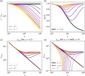


 Open access