2.1. Linear interaction analysis

Let us consider a two-dimensional, small amplitude planar vorticity wave with its wavenumber vector $\boldsymbol {k}$ inclined at an angle $\alpha$ with the $x$-axis (see figure 1). Mathematically, the vorticity wave can be represented as

(2.1)\begin{equation} \frac{\varOmega'}{k \bar{U}_1}={-}\textrm{i}\epsilon \exp({\textrm{i}(\boldsymbol{k} \boldsymbol{\cdot}\boldsymbol{r}-\omega t)}), \end{equation}

where $\boldsymbol {r}$ is the position vector, $k$ is the magnitude of the wavenumber vector and $\omega$ denotes the angular frequency of the vorticity wave. The quantity $\epsilon$ is the amplitude of the vorticity wave normalized by the wavenumber and mean velocity $\bar {U}_1$. The vorticity wave is advected by a one-dimensional, uniform mean flow of velocity towards the normal shock initially located along the $y$-axis. The shock deforms in response to the fluctuations and the local position of the unsteady shock is given by the function $\xi (y,t)$. The derivative $\xi _{y}$ thus represents the angular deformation of the shock (see figure 1).

Figure 1.

Schematic of the vorticity wave–normal shock interaction showing (a) the generation of acoustic and entropy waves downstream of the shock and (b) a magnified view of the shock deformation.

Small amplitude vorticity fluctuations are solenoidal fluctuations that impose a divergence-free condition on the fluctuating velocity field. The velocity fluctuations upstream of the shock (subscript 1) are given as

(2.2)$$\begin{gather} \frac{u'_1}{\bar{U}_1} = \epsilon \sin\alpha \exp({\textrm{i}k(x\cos{\alpha}+y\sin{\alpha})-\textrm{i}\omega t}), \end{gather}$$

(2.3)$$\begin{gather}\frac{v'_1}{\bar{U}_1} ={-}\epsilon \cos\alpha \exp({\textrm{i}k(x\cos{\alpha}+y\sin{\alpha})-\textrm{i}\omega t}), \end{gather}$$

where $u'$ and $v'$ represent the velocity fluctuations in the shock normal ($x$) and shock parallel ($y$) directions, respectively. Substituting the above forms in the linearized momentum equation shows that vorticity waves do not produce pressure fluctuations in the linear, inviscid limit. Physically, because vorticity fluctuations travel with the mean flow, they do not require pressure fluctuations to advect. Also, thermodynamics dictates that the vorticity wave does not create any fluctuations in entropy in the linear limit.

We investigate the interaction of such vorticity fluctuations with a normal shock and obtain the perturbation field downstream using LIA. We follow the works of Fabre et al. (Reference Fabre, Jacquin and Sesterhenn2001), Mahesh et al. (Reference Mahesh, Moin and Lele1996), Moore (Reference Moore1954) and Kovásznay (Reference Kovásznay1953), and the reader may refer to these for additional details on the theory. We perform this investigation for a constant specific heat ratio of air $\gamma =1.4$.

The incident vorticity wave refracts whereas acoustic and entropy waves are generated at the shock, with inclinations $\alpha ^{p}$ and $\alpha ^{s}$, respectively. The refracted vorticity wave has the same inclination as that of the downstream entropy wave. Let the wavenumber of the downstream acoustic and non-acoustic waves (vorticity and entropy) be $k^{p}$ and $k^{s}$, respectively. The post-shock acoustic wave can be either propagating or decaying depending on the angle of the incident wave. There exists a critical angle, $\alpha _{c}$ for $\alpha \in [0,{\rm \pi} /2]$, beyond which the acoustic waves decay immediately behind the shock.

The linearized Euler equations with the linearized R-H conditions as the boundary conditions at the shock are solved to obtain post-shock wave characteristics. The downstream fluctuations have the same $y$ and $t$ dependencies as the perturbed shock front (or the incident wave) as dictated by R-H conditions. The dispersion relation at the shock constrained by the continuity equation then yields that the transverse wavenumber and the angular frequency of the wave remain invariant across the shock. Thus, we get

(2.4)\begin{equation} \cot \alpha^s= r \cot \alpha, \end{equation}

where $r$ is the mean velocity ratio ($\bar {U}_{1} / \bar {U}_{2} = \bar {\rho }_{2} / \bar {\rho }_{1}$) across the shock. The ratio $r$ is an estimate of the amount by which the streamwise wavenumber of the vorticity wave gets compressed. The wavenumber for the acoustic wave $k^{p}$ is then determined from the acoustic wave equation; details are given by Mahesh et al. (Reference Mahesh, Lee, Lele and Moin1995).

The disturbance field downstream of the shock (subscript 2) can be written in terms of the vorticity fluctuations $\varOmega '_2$, entropy fluctuations $s'_2$ and pressure fluctuations $p'_2$ as

(2.5)$$\begin{gather} \frac{\varOmega_2'}{ k^s \bar{U}_2 }={-}\textrm{i}\epsilon Z_{vv} \exp({\textrm{i}k^s(x \cos\alpha^s + y \sin\alpha^s)-\textrm{i}\omega t}), \end{gather}$$

(2.6)$$\begin{gather}\frac{s_2'}{c_p}= \epsilon Z_{vs} \exp({\textrm{i}k^s(x \cos\alpha^s + y \sin\alpha^s)-\textrm{i}\omega t}), \end{gather}$$

(2.7)$$\begin{gather}\frac{p_2'}{\bar{P}_2} = \epsilon Z_{vp} \exp({\textrm{i}k^p(x \cos\alpha^p-\eta x + y \sin\alpha^p)-\textrm{i}\omega t}), \end{gather}$$

where $Z_{vv}$, $Z_{vs}$, $Z_{vp}$ are the corresponding transfer coefficients and are functions of $\alpha$ and $M_1$. The quantities $c_p$, $\bar {P}_2$ and $\eta$ represent the specific heat of fluid, mean pressure downstream of the shock and decay parameter of acoustic wave amplitude normal to the shock, respectively. Under the assumptions of LIA, decay of pressure perturbations at the shock ($\eta \neq 0$) occurs when $\alpha$ exceeds $\alpha _c$.

Both vorticity and acoustic modes of fluctuations generate velocity fluctuations downstream of the shock wave independent of each other in the linear limit. Accordingly, shock normal ($u_2'$) and shock parallel ($v_2'$) velocity fluctuations downstream can be written as

(2.8)$$\begin{gather} \frac{u_2'}{\bar{U}_2} = \epsilon \sin\alpha^sZ_{vv} \exp({\textrm{i}k^s(x \cos\alpha^s + y \sin\alpha^s)-\textrm{i}\omega t}) + \left\{\frac{\cos\alpha^p+ \textrm{i}\eta}{\gamma M_2 \zeta}\right\} \frac{p_2'}{\bar{P}_2}, \end{gather}$$

(2.9)$$\begin{gather}\frac{v_2'}{\bar{U}_2} ={-}\epsilon \cos\alpha^sZ_{vv} \exp({\textrm{i}k^s(x \cos\alpha^s + y \sin\alpha^s)-\textrm{i}\omega t}) + \left\{\frac{\sin\alpha^p}{\gamma M_2 \zeta}\right\} \frac{p_2'}{\bar{P}_2}, \end{gather}$$

where $\zeta$ is a function of the decaying parameter ($\eta$). The first and second terms on the right-hand side of (2.8) and 2.9 represent the contribution from vorticity mode and acoustic mode, respectively.

Corrugation of the shock measured with respect to its mean position is given as

(2.10)\begin{equation} k \xi = \epsilon Z_{v x} \exp({\textrm{i}k y \sin\alpha-\textrm{i}\omega t}), \end{equation}

where $Z_{vx}$ is the transfer coefficient for shock perturbation. Differentiating with respect to time gives the instantaneous shock corrugation speed in the streamwise direction:

(2.11)\begin{equation} \frac{\xi_t}{\bar{U}_1} ={-}\textrm{i}\epsilon \cos\alpha Z_{vx} \exp({\textrm{i}ky \sin\alpha-\textrm{i}\omega t}). \end{equation}

Substituting these expressions in the linearized Euler equations allows the estimation of the transfer coefficients of the disturbance ($Z_{vv}$, $Z_{vx}$, $Z_{vp}$ and $Z_{vs}$) for the post-shock regime. Mathematically, these transfer coefficients are computed as

(2.12)\begin{equation} A\left({\begin{array}{@{}c@{}} Z_{vv}\\ Z_{vs}\\ Z_{vp}\\ Z_{vx} \end{array}}\right)=\left(\begin{array}{@{}c@{}} -1 \\ -r\\ 0\\ \dfrac{r^2}{(\gamma - 1)M^2_1} \end{array}\right), \end{equation}

where

(2.13)\begin{equation} A = \left(\begin{array}{@{}ccccccc@{}} {\sin{\alpha^s}} & -1 & \dfrac{1}{\gamma}+ \dfrac{{\cos{\alpha^p}}+\textrm{i}\eta}{\gamma M_2 \zeta} & \textrm{i}(r-1){\cos{\alpha^p}}\\ 2{\sin{\alpha^s}} & -1 & \dfrac{M^2_2+1}{\gamma M^2_2}+ \dfrac{{\cos{\alpha^p}}+\textrm{i}\eta}{\gamma M_2 \zeta} & 0 \\ -{\cos{\alpha^s}} & 0 & \dfrac{ {\sin{\alpha^p}}}{\gamma M_2 \zeta} & \textrm{i}(1-r){\sin{\alpha}}\\ {\sin{\alpha^s}} & \dfrac{1}{(\gamma-1)M^2_2} & \dfrac{1}{\gamma M^2_2}+ \dfrac{{\cos{\alpha^p}}+\textrm{i}\eta}{\gamma M_2 \zeta} & \textrm{i}r(r-1){\cos{\alpha^p}} \end{array}\right). \end{equation}

Figure 2(a) shows the variation of the transfer coefficients with $\alpha$ for a fixed $M_1$. The transfer coefficients for vorticity $Z_{vv}$ and shock deformation $Z_{vx}$ show a monotonic increase with $\alpha$ in the propagating regime ($\alpha <\alpha _c$), reaching a maximum at $\alpha _c$. They decrease with further increase of $\alpha$ in the decaying regime. Transfer coefficients for pressure and entropy have a non-monotonic variation in the propagative regime. For all $M_1$ and $\alpha$, LIA predicts that $Z_{vv}$ is the largest, which indicates that the linear processes are dominated by vorticity amplification (see figures 2(a) and 2(b)). In the limit of a vanishing shock wave ($M_1 = 1$), there is no amplification of vorticity ($Z_{vv} =1$) and $Z_{vv}$ increases in magnitude for increases in $M_1$ to reach an asymptotic value as $M_1 \to \infty$.

Figure 2.

Variation of transfer coefficients with (a) $\alpha$ at $M_1=3$ and (b) $M_1$ at $\alpha =30^\circ$. Dashed red line in panel (a) indicates $\alpha _c$.

The relative magnitude of the transfer coefficients and their variation with $\alpha$ and $M_1$ play an important role in the weakly nonlinear framework (WNLF) presented subsequently. The high values of $Z_{vv}$ and $Z_{vx}$ in the vicinity of $\alpha _c$ degrade the accuracy of the numerical solution presented in the paper. Hence, we restrict our numerical simulations to low values of $\alpha$ in the propagating regime away from $\alpha _c$.

2.2. Numerical simulations

The interaction of the vorticity wave with a normal shock is studied numerically over a two-dimensional domain, as shown in figure 3. The length of the computational domain is $4{\rm \pi}$ and $2{\rm \pi}$ in the streamwise ($x$) and transverse ($y$) directions, respectively. Four stations in the $x$-direction are marked in figure 3. We specify a supersonic boundary condition for the inflow station ($x=-{\rm \pi}$), where velocity fluctuations

(2.14)$$\begin{gather} u^\prime = \epsilon \bar{U}_1 \sin \alpha \cos(k\sin \alpha y-\omega t), \end{gather}$$

(2.15)$$\begin{gather}v^\prime ={-}\epsilon \bar{U}_1 \cos \alpha \cos( k\sin \alpha y-\omega t), \end{gather}$$

are superimposed on a one-dimensional supersonic streamwise mean flow $\bar {U}_1$. A non-reflecting subsonic boundary condition is applied at the outflow ($x=3{\rm \pi}$) and a periodic boundary condition is used for the transverse boundaries.

Figure 3.

Numerical domain: $x=-{\rm \pi}$ shows the inlet boundary; $x=0$ is the initial position of the normal shock; $x=2{\rm \pi}$ the start of a numerical sponge; and $x=3{\rm \pi}$ the outlet boundary and end of the numerical sponge.

The flow downstream of the normal shock is subsonic and allows spurious acoustic waves from the outflow boundary to propagate towards the shock. These acoustic reflections are undesirable and need to be avoided or damped. A numerical sponge similar to that prescribed by Larsson & Lele (Reference Larsson and Lele2009) and Sethuraman et al. (Reference Sethuraman, Sinha and Larsson2018) is used to achieve this. In our numerical domain, a sponge is used from $x=2{\rm \pi}$ to $x=3{\rm \pi}$ and it dampens the fluctuations to a target state defined by the R-H conditions for the mean flow.

Compressible Euler equations for an ideal gas ($\gamma =1.4$) are solved for various $M_1$ using the solution-adaptive finite-difference Hybrid code (Larsson & Lele Reference Larsson and Lele2009). A fifth-order accurate WENO scheme with Roe-flux splitting is used to calculate the approximate fluxes near the shock and a sixth-order accurate central difference scheme is used for the remainder of the domain. The system of equations is integrated in time using a fourth-order accurate, explicit Runge–Kutta (RK4) scheme. Numerical shock is identified using a modified Ducros sensor (Larsson & Lele Reference Larsson and Lele2009). The shock is identified as the region where negative dilatation is greater than the low-pass filtered vorticity magnitude. This numerical procedure has been verified and validated on various problems of interest (Larsson & Lele Reference Larsson and Lele2009; Johnsen et al. Reference Johnsen2010; Larsson et al. Reference Larsson, Bermejo-Moreno and Lele2013), and additional details about the code can be found in Sethuraman et al. (Reference Sethuraman, Sinha and Larsson2018), Bermejo-Moreno et al. (Reference Bermejo-Moreno, Bodart, Larsson, Barney, Nichols and Jones2013), Larsson et al. (Reference Larsson, Bermejo-Moreno and Lele2013) and Larsson & Lele (Reference Larsson and Lele2009).

Flow variables are normalized so that the upstream velocity equals the upstream Mach number ($M_1$). For this purpose, we use density and sound speed upstream of the shock as characteristic variables, whereas the $y$-component of wavenumber ($k_y$) is used to normalize different length scales. Pressure is normalized using the characteristic density and sound speed, whereas vorticity is normalized using $k_y$ and sound speed upstream of the shock. The equations are integrated in time with a Courant–Friedrichs–Lewy (CFL) number of 0.8, which corresponds to a flow time scale of $\sim$0.003. It takes approximately 200 to 300 time steps to simulate one wave passage through the shock.

Initially, the normal shock lies at $x=0$ and oscillates in the transverse direction when fluctuations impinge on it and change the downstream pressure. Mismatch in the pressure levels downstream of the shock with that obtained from R-H conditions causes the shock to drift slowly. We use a time-dependent back-pressure controller (Larsson & Lele Reference Larsson and Lele2009) to reduce the shock movement and make it as stationary as possible around the desired location, $x=0$. We follow the implementation procedure prescribed by Sethuraman et al. (Reference Sethuraman, Sinha and Larsson2018) to control the movement of the shock using the back-pressure controller.

The time taken by the initial disturbances to adjust to the boundary conditions is considered as an initial transient. We track the shock movement during this time as in Sethuraman et al. (Reference Sethuraman, Sinha and Larsson2018) to ascertain that the post-shock statistics are computed after the initial transients have passed. The flow statistics achieve a steady-state value at this point.

Post-shock statistics are collected at a fixed $x$-location by averaging over the transverse ($y$) direction and time. For averaging, 61 time realizations distributed uniformly over a wave period are used. Flow statistics change negligibly when the averaging time is increased to multiple wave periods from those obtained over one wave period. This signifies that the statistics evaluated over one wave period are sufficiently time-independent, and the initial transients in the numerical simulations have vanished.

Figure 4(a) shows the variation of the root-mean-squared value of fluctuation kinetic energy (FKE) downstream of the shock computed for four different grid resolutions. The data are normalized by its upstream value to obtain the amplification across the shock. We observe a systematic grid-convergence to the finest grid and the LIA solution. We also note that FKE has a wave-like variation behind the shock. This is because post-shock velocity fluctuations have contribution both from vorticity and acoustic modes. The difference in wavenumbers of the two modes result in a periodic variation of FKE. In comparison, the upstream FKE is constant as it has contribution only from the vorticity mode.

Figure 4.

Effect of grid refinement on (a) the amplification of root-mean-squared fluctuation kinetic energy (FKE) and (b) the amplification of root-mean-squared value of vorticity and FKE across the shock. Here, $N_x$ is the number of points in the streamwise direction; $M_1=1.75$, $\alpha =30^\circ$ and $\epsilon =0.1$.

In figure 4(b), the amplification of the root-mean-squared value of FKE and vorticity ($\varOmega$) averaged in the transverse direction and in time as well as over one wavelength of the post-shock variation is presented for four successively refined computational grids. The data show negligible change for grid sizes $800\times 128$ and above. Therefore, we choose a grid size of $800\times 128$ for our study and all subsequent numerical results presented are generated using this grid. The grid refinement study was performed for $M_1= 1.75$ and $\alpha = 30^\circ$. Comparable results are obtained (not shown) for the entire range of parameters considered in this work.

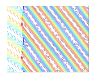
Figure 5 shows the vorticity contours computed for the shock–vorticity wave interaction at $\alpha = 30^\circ$ and $M_1 = 1.5$. Two values of $\epsilon$ are used to highlight the effect of upstream vorticity amplitude. The numerical solution for $\epsilon = 0.01$ matches the vorticity pattern shown in figure 1, in terms of the refraction of the waves at the shock and the sinusoidal deformation of the shock wave. The parallel contour lines indicate two-dimensional planar waves as predicted by LIA. In comparison, the higher-amplitude interaction ($\epsilon =0.25$) shows deviation from the LIA solution downstream of the shock. The non-parallel vorticity contours, especially close to vorticity minima (around $-$2) indicate that the numerical solution is not a sinusoidal wave. The objective of this work is to study these nonlinear effects immediately downstream of the shock using the weakly nonlinear framework presented below.

Figure 5.

Vorticity contour plots at $\alpha = 30^\circ$ and $M_1 = 1.5$ for (a) $\epsilon =0.01$ and (b) $\epsilon =0.25$. The interaction and refraction of the vorticity wave with the shock are clearly visible. The amplitude of shock fluctuations and the nonlinearities in the downstream vorticity are larger for larger $\epsilon$.

4.1. Comparison with numerical simulations

Variation of $\sigma _N$ is shown in figure 12 for $\alpha = \{20^\circ,30^\circ,40^\circ \}$, for $\epsilon$ ranging from $0.01$ to $0.25$ and $M_1=\{1.25, 1.5, 1.75, 2 \}$. We notice that $\sigma _N$ for all the cases considered increases with $\epsilon$ and $M_1$ for a given $\alpha$. The nonlinear effects are significant at higher $\epsilon$ and $M_1$ owing to the modal interaction at a given $\alpha$. The results agree with the assertion of the modal interaction made by Chu & Kovásznay (Reference Chu and Kovásznay1958) with a problem involving a shock wave for the first time.

Figure 12.

Variation of $\sigma _N$ with $\epsilon$ at $M_1=1.25$ (square), $M_1=1.5$ (triangle), $M_1=1.75$ (pentagon) and $M_1=2$ (circle) for: (a) $\alpha =20^\circ$; (b) $\alpha =30^\circ$ and (c) $\alpha =40^\circ$.

We compare the deviation of the numerical solution from LIA with the second-order effects predicted by the weakly nonlinear framework in figure 13. Note that the nonlinear effects in numerical simulation $\sigma _N$ are a function of $\epsilon$, $M_1$ and $\alpha$. However, $\phi$ includes the theoretical second-order effects of $M_1$ and $\alpha$, while the $\epsilon ^2$ variation of $\varOmega _2^{(2)}$ is taken out from the definition of $\phi$. We plot the ratio $\sigma _N/\phi$ to study the effect of $M_1$ and $\alpha$ on the higher-order vorticity generated by the shock wave. Figure 13 shows that the Mach number variation of $\sigma _N$ is collapsed by the ratio $\sigma _N /\phi$ and the data show a clear trend of $\epsilon ^2$ variation at higher $\epsilon$ values. There is a systematic deviation towards $\epsilon$ scaling in the low amplitude range and it is discussed subsequently. The $\epsilon ^2$ scaling is a direct prediction of weakly nonlinear framework and the numerical data support this finding. Moreover, the collapse of the data (for each $\alpha$) shows that the Mach number scaling predicted by the theory also holds for the numerical solutions. The same is true for the $\alpha$ scaling shown in figure 14. The deviation of the numerical solution from LIA results collapse to a single curve when scaled by the second-order vorticity magnitude obtained from the weakly nonlinear framework. This collapse proves the validity of the weakly nonlinear framework.

Figure 13.

Comparison of WNLF predictions and numerical simulations results. Variation of $\sigma _N/\phi$ for $M_1=1.25$ (square), $M_1=1.5$ (triangle), $M_1=1.75$ (pentagon) and $M_1=2$ (circle) for: (a) $\alpha =20^\circ$; (b) $\alpha =30^\circ$ and (c) $\alpha =40^\circ$. The variation of $\sigma _N$ with $\epsilon$ collapses to a single curve when scaled by the magnitude of $\phi$. Lines show the $\epsilon ^2$ (solid) and $\epsilon$ (dashed) variation.

Figure 14.

Collapse of the numerical data with respect to incidence angle: the ratio $\sigma _N/\phi$ for different $\alpha$ ($20^\circ$ square, $30^\circ$ triangle and $40^\circ$ circle) plotted against $\epsilon$ for different Mach numbers. Lines show the $\epsilon ^2$ (solid) and $\epsilon$ (dashed) variation with (a) $M_1=1.5$ and (b) $M_1=2$.

Figure 15 plots the difference between $\sigma _N$ and $\phi$ at various $M_1$ and $\alpha$; the data are once again scaled by $\phi$. It is observed that the difference is in the range $10^{-2}$ to $10^{-4}$ and approximately varies linearly with $\epsilon$. Although the difference is small in magnitude compared with the data presented in figures 13 and 14, it is important to investigate the reasons behind this discrepancy.

Figure 15.

The absolute error $| \sigma _N - \phi |$ scaled by $\phi$ plotted as a function of $\epsilon$ (a) for varying $M_1$ (1.25, square; 1.5, triangle; 1.75, pentagon and 2.0, circle) for $\alpha =20^\circ$ and (b) for varying $\alpha$ ($20^\circ$, square; $30^\circ$, triangle and $40^\circ$, circle) at $M_1=2$. Line represents the $\epsilon$ variation.

The discrepancies between $\sigma _N$ and $\phi$ are possibly related to the numerical challenges faced in the computations and the procedure used to evaluate $\sigma _N$. The error related to numerical techniques are discussed by Johnsen et al. (Reference Johnsen2010) and have been minimized while carrying out this study. The selection of the $x$ location used to calculate $\sigma _N$ downstream of the shock and the phase difference between theoretical and numerical waves upstream of the shock contributes to some error. We ensure that we minimize these errors and it is found to be of the order of $10^{-5}$ or smaller.

Finally, and perhaps more significantly, the numerical simulations capture the unsteady oscillating shock wave on a Cartesian computational grid. This introduces errors in shock capturing owing to misalignment between the shock shape and the grid lines (Ching et al. Reference Ching, Lv, Gnoffo, Barnhardt and Ihme2019; Kitamura Reference Kitamura2013), and creates discrete jumps in the shock profile, as shown in figure 16. Note that the figure is highly magnified in the vicinity of the shock wave, such that the shock profile over two grid cells is clearly visible in terms of the pressure contours. The magnification in the $x$-direction exceeds that in the $y$-direction by a factor of 5. Each jump introduces an additional curvature to the numerically captured shock wave, and it generates non-physical vorticity, entropy and related quantities behind the shock. It is observed that the number of jumps in the shock wave increases proportionately with the amplitude of the shock motion (compare figures 16(a) and 16(b)). The shock amplitude, in turn, is proportional to the amplitude of the incoming vorticity wave ($\epsilon$), as per the assumption in linear theory. The shock-grid misalignment error can therefore be expected to scale linearly with $\epsilon$, denoted by the dashed lines in figure 15.

Figure 16.

Pressure contours show corrugations in the numerically captured shock wave on a Cartesian grid leading to shock–grid misalignment error for $\alpha =25^\circ$ and $M_1=1.5$: (a) $\epsilon =0.1\,\%$; (b) $\epsilon =0.2\,\%$.

Note that the sinusoidal deformation of the shock wave is an inherent feature of the shock–vorticity wave interaction. It cannot be neglected even at low values of $\epsilon$. The shock-capturing error is therefore small, but finite at low $\epsilon$. As we increase the amplitude of the upstream vorticity wave, higher-order effects become important and the scaling shifts from $O(\epsilon )$ to $O(\epsilon ^2)$ (see figures 13 and 14). After removing the $O(\epsilon )$ error shown in figure 15, the variation of the corrected $\sigma _N/ \phi$ is plotted in figures 17 and 18. We find that the scaled variation now varies clearly as $O(\epsilon ^2)$ over the entire range of parameters considered in this work.

Figure 17.

Collapse with respect to $M_1$: the ratio $\sigma _N/\phi$ after removing $O(\epsilon )$ error for different $\alpha$ ($20^\circ$, square; $30^\circ$, triangle and $40^\circ$, circle) plotted against $\epsilon$ for different Mach number. Line shows the $\epsilon ^2$ variation.

Figure 18.

Variation for $\sigma _N$ scaled by the magnitude of $\phi$ with $\epsilon$ after removing $O(\epsilon )$ error for $\alpha =20^\circ$ (square), $\alpha =30^\circ$ (triangle) and $\alpha =40^\circ$ (circle) for (a) $M_1=1.25$, (b) $M_1=1.5$, (c) $M_1=1.75$, (d) $M_1=2$. Solid line shows $\epsilon ^2$ variation.

The magnitude of $\phi$ constitutes the nonlinear effects in vorticity as given by (3.8) and follows the trend of $\sigma _N$ accurately after correcting for numerical error. This means that the physics which governs nonlinear effects in vorticity as a function of $M_1$ is captured by $\phi$ in the weakly nonlinear range of $\epsilon \leq 0.25$. These results strongly confirm the usefulness of the weakly nonlinear framework presented in § 3.1, which is correct up to second-order in $\epsilon$.

It is important to study the scaling of these nonlinear effects with respect to $M_1$. Existence of scaling allows the predictions of variations at different $M_1$ without performing numerical simulations for each individual case. The results from LIA can also be improved by offsetting for the error accordingly. Scaling could be valuable for problems of the shock–turbulence interaction, where DNS of the problem at higher $M_1$ becomes increasingly more difficult to perform.

4.2. Parameter space

The weakly nonlinear framework presented in this work uses the results of LIA to study the nonlinear effects in the shock–vorticity interaction. As per LIA, the shock-downstream disturbance field is a function of the upstream vorticity wave amplitude $\epsilon$, incidence angle $\alpha$ and the shock strength given by the flow Mach number $M_1$. We consider these three parameters for characterizing the nonlinear effects. The results from linear theory also depend on the wavenumber of the upstream wave. Here, we keep the transverse component of the upstream wavenumber constant ($k_y = 2$). Therefore, the upstream wavenumber $k = k_y/\sin \alpha$ changes with the incidence angle.

Nonlinear effects in the shock–disturbance interactions are primarily driven by the intensity of fluctuations ($\epsilon$) upstream of the shock. The separation of linear and nonlinear regimes based on $\epsilon$ is not clearly defined for such interactions. Here, we use existing literature on the shock–turbulence interaction to guide the choice of the range of $\epsilon$ used to study the nonlinear effects. Canonical shock–turbulence interactions are classified as lying in either a wrinkled regime or a broken shock regime. At low disturbance intensities, the shock front remains intact but has unsteady corrugation. At large values of turbulence intensities, the shock front may disappear locally, giving rise to what are called as shock holes. LIA does not predict shock holes and is therefore valid only in the wrinkled regime. The same is expected to be true for the weakly nonlinear framework that builds upon the LIA solution.

The criteria $M_t/(M_1-1) = 0.6$ given by Donzis (Reference Donzis2012b) is often used to demarcate the wrinkled and broken-shock regimes, where $M_t$ is the turbulent Mach number that quantifies the intensity of the upstream turbulent fluctuations. It is related to the vorticity wave amplitude $\epsilon$ as $M_t = \epsilon M_1$. We restrict the range of $\epsilon$ in our study to meet this criteria for wrinkled shock interaction. For the chosen range of Mach numbers between 1.25 and 2.0, this gives the maximum value of $\epsilon$ to be between 0.12 and 0.3. We thus choose $\epsilon$ to vary between 0.01 and 0.25 to study the weakly nonlinear effects at the shock wave. As per (3.9), the normalized second-order vorticity $\varOmega _2^{(2)}$ is proportional to $\epsilon ^2 \phi$, where $\phi$ is $O(1)$. The deviation of the numerical solution from LIA is therefore expected to have a magnitude $\epsilon ^2 \sim 0.06$ as can be observed from figure 12.

The nonlinearity at the shock wave is also driven by inter-modal interaction, as noted in § 3. In the current study, the upstream disturbance field is purely vortical, while the downstream disturbances include vorticity, acoustic and entropy modes. As per the LIA, amplification across the shock is characterized by the transfer coefficients plotted in figure 2. We note the high values of $Z_{vv}$ and $Z_{vx}$ in the vicinity of the critical incidence $\alpha _c$, which can limit the applicability of LIA and the weakly nonlinear framework. The value of $\alpha _c$ is approximately $62^\circ$ for the range of Mach numbers considered here, and we restrict the range of $\alpha$ to approximately $60^\circ$. The results for $\alpha = 20^\circ \unicode{x2013}40^\circ$ are presented in § 4.1, while the higher values of $\alpha$ are discussed in § 5.

We use the weakly nonlinear framework to explore second-order vorticity for Mach numbers up to 5. The LIA transfer coefficients are found to reach close to their asymptotic values in the hypersonic regime. The same is expected to hold for $\varOmega _2^{(2)}$. The comparison with numerical solution (§ 4.1) is limited to Mach 2, primarily owing to the limitations of the numerical methodology. The shock-grid misalignment error increases with shock strength, which makes it difficult to perform a meaningful comparison with the theoretical predictions. The same is true for incidence angles $\alpha$ beyond $40^\circ$ and in the decaying regime ($\alpha > \alpha _c$).

The Mach number range from 1.25 to 2.0 is important in many high-speed flow applications. The Mach number in a scramjet combustor is in this range, where shock-induced mixing is important for efficient combustion. Shock–boundary layer interactions in hypersonic intakes may have a higher Mach number at the boundary layer edge, but the shock waves are highly inclined to the flow. The shock-normal Mach number is much lower, often in the range of 1–2 for a free stream Mach number of 5 (Schulein Reference Schulein2006) and even as high as 13 (Pasha & Sinha Reference Pasha and Sinha2012). Also, experiments studying the shock–turbulence interaction in wind tunnels are conducted in the low supersonic range because it is difficult and expensive to conduct them at higher $M_1$.

5.1. LIA limit

The applicability of LIA is evaluated by comparing the magnitude of the LIA-predicted vorticity ($\varOmega _2^{(1)}$) given by (3.7a) and that of the second-order effect ($\varOmega _2^{(2)}$) given by WNLF in (3.8). LIA is expected to be valid when

(5.1)\begin{equation} \varOmega_2^{(2)} \ll \varOmega_2^{(1)}. \end{equation}

We have from (3.9), $\phi = {|\varOmega _2^{(2)}|}/{\epsilon ^2\bar {U}_1k}$. Let us define $\psi$ as

(5.2)\begin{equation} \psi = \frac{|\varOmega_2^{(1)}|}{\epsilon \bar{U}_1k}. \end{equation}

We plot the ratio $\phi /\psi$ as a function of $M_1$, for different $\alpha$, in figure 19(a). As $M_1$ is increased, for a given $\alpha$, we observe that the ratio at first increases, reaches a maximum value and then decreases to attain an asymptotic limit in the hypersonic range. This can be understood in terms of the variation of the linear and second-order vorticity with Mach number, as discussed below.

Figure 19.

Nonlinear effects in vorticity amplification represented using (a) a relative measure $\phi /\psi$, (b) an absolute measure $\epsilon _{limit}$.

The ratio $\phi /\psi$ approaches zero in the limit $M_1 \to 1$, as $\phi \to 0$ and $\psi \to 1$. This is because

(5.3)\begin{equation} \varOmega^{(1)}_2 \to \varOmega^{(1)}_1 \neq 0 \quad \text{whereas}\ \varOmega_2^{(2)} \to 0, \end{equation}

in this limit. In other words, the vorticity amplitude remains unaltered across an infinitely weak shock, which results in a finite value of the downstream linear vorticity. By comparison, the second-order vorticity becomes negligible in magnitude in the sonic limit. This is because $u'_1 = u'_2$, $\varOmega '_1 = \varOmega '_2$ and $\xi _t = \xi _y = 0$ for a vanishing shock wave. Thus, the contribution of $\varOmega _a$ in (3.8) drops out and there is no net turbulent transport in the case of an infinitely weak shock wave. The other terms $\varOmega _b = \varOmega _c = 0$ by virtue of $\xi _{yy} = 0$ and $r = 1$, respectively, which results in a vanishing value of the second-order vorticity in this limit.

Using Taylor series expansion of $\phi$ and $\psi$ in the vicinity of the sonic point and retaining only the first-order term in Mach number, we can write

(5.4)\begin{equation} \frac{\phi}{\psi} = \frac{\phi'(M_1-1)}{1 + \psi^{\prime}(M_1-1)} \approx \phi^\prime (M_1-1) + O(M_1 -1)^2, \end{equation}

where $\phi ^\prime$ and $\psi ^\prime$ represent the derivative with respect to Mach number of the corresponding function. The slope of the ratio $\phi /\psi$ in figure 19(a) is therefore determined by the derivative $\phi ^\prime$. For weak shocks, the second-order vorticity increases in magnitude with increasing Mach number (see figure 7). Thus, the derivative $\phi ^\prime$ is positive, and it increases with $\alpha$ in the propagating regime. However, the initial slope of $\psi$ at $M_1 = 1$ is independent of Mach number, as

(5.5)\begin{equation} \psi = Z_{vv} \propto r, \end{equation}

and

(5.6)\begin{equation} \lim_{M_1\to1} \frac{\textrm{d}\psi}{\textrm{d} M_1} = \lim_{M_1\to1} \frac{\textrm{d} r}{\textrm{d} M_1} = \frac{4}{\gamma+1}. \end{equation}

The limiting slopes $\phi ^\prime$ and $\psi ^\prime$ are plotted as a function of $\alpha$ in figure 20. Together, they give an increasing trend for the ratio $\phi /\psi$ for Mach numbers close to 1. However, although both $\varOmega _2^{(2)}$ and $\varOmega _2^{(1)}$ reach asymptotic values in the large $M_1$ limit, the growth of $\varOmega _2^{(2)}$ becomes smaller as $M_1$ increases and reaches an asymptotic limit for smaller $M_1$ when compared with $\varOmega _2^{(1)}$ (see figures 6 and 7 which plot $\phi$ and $\psi$). This results in a decreasing trend for $\phi /\psi$ for Mach numbers beyond 2, as is observed in figure 19(a). In the large $M_1$ limit, this ratio reaches an asymptotic value that depends only on $\alpha$. Thus, we get a local peak in $\phi /\psi$, which corresponds to the Mach number, where the second-order effects are the largest compared with the first-order vorticity amplification, once the amplitude factors are scaled out.

Figure 20.

The slope of $\phi$ and $\psi$ in the limit of $M_1 \to 1$ as a function of incidence angle $\alpha$.

The ratio $\phi /\psi$ is also observed to increase with the incidence angle $\alpha$ (not shown). This behaviour in the low-Mach-number regime is in line with the results presented in figure 12 of § 4, whereas the variation for large Mach numbers is predicted using the weakly nonlinear framework presented in § 3. In short, the LIA prediction of vorticity amplification increases with $\alpha$, as per the variation of $Z_{vv}$ shown in figure 2(a). In comparison, $\varOmega _2^{(2)}$ varies as the product of two transfer coefficients, such as $Z_{vv}Z_{vp}$ or $Z_{vv}Z_{vv}$ (as per (3.7b)) resulting in the observed trend in figure 2(a).

Next, we rewrite (5.1) in terms of the functions $\phi$ and $\psi$ to arrive at a limit on $\epsilon$ for LIA to be valid,

(5.7)\begin{equation} \epsilon_{limit} = 0.1\frac{\psi}{\phi}. \end{equation}

Here, a factor of 0.1 is introduced to change the inequality to equality under the assumption that the second-order vorticity is less than or equal to $10\,\%$ of the linear vorticity in magnitude. This corresponds to a maximum of $10\,\%$ error in LIA results.

Figure 19(b) shows the variation of $\epsilon _{limit}$ with $M_1$ for various $\alpha$ values evaluated using (5.7). As expected, the variation of $\epsilon _{limit}$ with $M_1$ at a given $\alpha$ is non-monotonic. It decreases with increasing $M_1$ for weak shocks, reaches a local minima and subsequently increases for higher Mach numbers. It is opposite to the trend observed in figure 19(a), where the ratio $\phi /\psi$ gives the relative measure of nonlinearity in vorticity. However, figure 19(b) provides an absolute quantitative limit on the upstream vorticity wave amplitude as a function of flow parameters. At a given $\alpha$ and $M_1$, $\epsilon$ values above $\epsilon _{limit}$ would breach the limit of LIA validity, which results in the prediction that have more than $10\,\%$ error.

The minimum value of $\epsilon _{limit}$ is attained at $M_1 \simeq 2$ for the different $\alpha$ values shown in figure 19(b). This poses the strictest limit on the range of upstream vorticity magnitude $\epsilon$ for which LIA results are accurate. At lower Mach numbers ($M_1 < 2$), higher values of $\epsilon$ are permissible. In fact, the $\epsilon _{limit}$ curves have a singular behaviour at $M_1 = 1$. This can be resolved by noting the limiting behaviour of the first-order vorticity and the second-order vorticity given in (5.3).

As noted above, $\epsilon _{limit}$ increases with Mach number for $M_1 > 2$, which implies that LIA is valid for a larger range of $\epsilon$ at higher Mach numbers, or equivalently, for stronger shock waves. The mean compression of the shock amplifies vorticity disturbances in the flow and this linear effect is accurately predicted by LIA. A stronger shock leads to a higher amplification of vorticity amplitude. However, the second-order vorticity is generated by nonlinear effects owing to the inter-modal interaction and shock-curvature effects, as per the weakly nonlinear framework. The amplitude of the downstream Kovásznay modes and the shock oscillation both depend on the disturbance level upstream of the shock. The $\epsilon _{limit}$ in figure 19(b) can thus be interpreted as a balance between two competing effects. A stronger shock favours the linear effect owing to the mean compression of the shock, while larger amplitude disturbance (higher $\epsilon$) increases the nonlinear contribution. For a given Mach number, the value of $\epsilon _{limit}$ is a function of the vorticity wave incidence angle. For the different values of $\alpha$ presented in figure 19(b), $\epsilon _{limit}$ increases monotonically at higher Mach numbers, which indicates that LIA has a higher range of validity for strong shock waves.

The validity of LIA for the shock–turbulence interaction is usually prescribed in terms of $M_t$ and $M_1$. For example, the criteria $M_t/(M_1-1) = 0.6$ is frequently used to demarcate the wrinkled regime and broken shock interactions (Donzis Reference Donzis2012b). The $\epsilon _{limit}$ presented above can be interpreted in a similar vein by noting that $\epsilon = M_t/M_1$, such that the values plotted in figure 19(b) give an upper limit on the ratio of $M_t$ to $M_1$ for the validity of LIA for the shock–vorticity wave interaction. As per the weakly nonlinear framework, this limit is a function of the incidence angle and shock strength. For a given Mach number, (5.7) can be integrated over all possible $\alpha$ (in three-dimensional space) to get an estimate of $\epsilon _{limit}$ for the shock–turbulence interaction. Further, the limit is derived based on the magnitude of the second-order vorticity. It may be different if we consider nonlinear effects in other quantities like Reynolds stresses and downstream pressure fluctuations. The weakly nonlinear framework can be extended to study other quantities of interest to get a more general criterion for the validity of LIA.

5.2. Second-order effects at high $M_1$ and $\alpha$

We use the expressions derived in § 3 to analyse the nonlinear effects in vorticity amplification for high $\alpha$ and $M_1$ regime to understand the underlying physics better. Figure 21 shows that the second-order vorticity increases with Mach number ($M_1$) and reaches an asymptotic value in the hypersonic limit. However, $\phi$ exhibits a sharp increase near $\alpha _c$, by approximately a factor of 10 compared with its value at $\alpha = 30^\circ$ considered in § 4.

Figure 21.

Variation of $\varOmega _2^{(2)}$ from (3.8) (circle), $\varOmega _a+\varOmega _b$ (dashed line) and $\varOmega _a+\varOmega _b+\varOmega _c$ (triangle) with (a) $M_1$ at $\alpha =60^\circ$, (b) $\alpha$ at $M_1=3$.

Figure 22 plots the variation of the constituent terms $\varOmega _a$, $\varOmega _b$ and $\varOmega _c$ of the second-order vorticity as a function of $M_1$ and $\alpha$. At low values of $\alpha$ (see figure 22a), the second-order vorticity is dominated by the turbulent transport term $\varOmega _a$ and the shock-curvature effect $\varOmega _b$. The $\varOmega _c$ term is comparatively small in magnitude and was neglected in the analysis presented earlier. The $\varOmega _c$ constitutes the additional effect of the turbulent flux of vorticity and shock-curvature along with dilatation, which becomes significant at $\alpha$ close to $\alpha _c$. The nonlinear effects at $\alpha$ close to $\alpha _c$ is dominated by $\varOmega _b$ (see figure 22b). The other parts, $\varOmega _a$ and $\varOmega _c$, have a non-negligible contribution to second-order vorticity at such high $\alpha$. The dramatic rise in $\varOmega _b$ for high incidence angles is also visible in figures 22(c) and 22(d), which plot the variation of the constituent terms at $M_1 = 1.75$ and $5$, respectively.

Figure 22.

Variation of the magnitude of $\varOmega _a$ (circle), $\varOmega _b$ (triangle) and $\varOmega _c$ (square) from (3.8) with $M_1$: (a) at $\alpha =30^\circ$; (b) at $\alpha =60^\circ$ and with $\alpha$ (c) at $M_1=1.75$; (d) at $M_1= 5$.

The variation of $\varOmega ^{(2)}_2$ and its constituent terms at high $\alpha$ can be interpreted in terms of the transfer coefficients presented in figure 2(a). Both $Z_{vv}$ and $Z_{vx}$ show a sharp rise in the vicinity of the critical angle and all the transfer coefficients, including $Z_{vp}$, have singular behaviour at $\alpha _c$. The resulting intermodal interaction terms in (3.10) and (3.11) also show a similar behaviour, and this would severely restrict the validity of LIA at the critical angle.