


1. Introduction
Stirring and mixing results from the combined action of differential advection and molecular diffusion on a material quantity (Thiffeault Reference Thiffeault2008), and is a ubiquitous process in geophysical, environmental and industrial fluids (see e.g. Faller & Auer Reference Faller and Auer1988; Biferale et al. Reference Biferale, Crisanti, Vergassola and Vulpiani1995; Seo & Cheong Reference Seo and Cheong1998; Haynes & Shuckburgh Reference Haynes and Shuckburgh2000; Neuman & Tartakovsky Reference Neuman and Tartakovsky2009; Boano et al. Reference Boano, Harvey, Marion, Packman, Revelli, Ridolfi and Wörman2014; Van Sebille et al. Reference Van Sebille2018). Despite its importance, a complete analytical description of stirring and mixing remains an open problem owing to the complex interplay between differential advection, diffusion and the multiscale nature of the problem, highlighted by the multifractal behaviour that the scalar field exhibits even when advection is a spatially smooth function of space, usually a single Fourier mode (Aref Reference Aref1984; Pierrehumbert Reference Pierrehumbert1994; Antonsen et al. Reference Antonsen, Fan, Ott and Garcia-Lopez1996; De Moura Reference De Moura2014).
The evolution of a scalar tracer under the combined effect of molecular mixing and stirring is given by the advection–diffusion equation, written in the absence of sources and sinks as
 \begin{equation} \frac{\partial\theta}{\partial t} + \boldsymbol{u} \boldsymbol{\cdot}\boldsymbol{\nabla}\theta = \kappa\,\nabla^2\theta, \end{equation}
where  $\kappa$ is the molecular diffusivity, and $\boldsymbol {u}$ is a time-varying, non-divergent velocity field. The tracer concentration $\theta$ is considered dynamically passive when its evolution has no effect on the inertia of the flow so that the velocity $\boldsymbol {u}$ is prescribed (although $\boldsymbol {u}$ need not solve the Navier–Stokes equations; Majda & Kramer Reference Majda and Kramer1999). From a theoretical point of view, (1.1) provides the simplest example of a linear non-self-adjoint operator, which is ubiquitous in many physical sciences (Miri & Alu Reference Miri and Alu2019), and whose qualitative properties are not fully understood (Childress & Gilbert Reference Childress and Gilbert1995; Sukhatme & Pierrehumbert Reference Sukhatme and Pierrehumbert2002; Giona et al. Reference Giona, Adrover, Cerbelli and Vitacolonna2004). Furthermore, the study of stirring and mixing via (1.1) offers many of the same mathematical challenges as the study of fluid turbulence while remaining a linear and therefore less complicated physical model (Pierrehumbert Reference Pierrehumbert2000).
In this study, we compute the spectra of the operator (1.1) and use it to study the properties and behaviour of analytical solutions in a doubly periodic domain with arbitrary initial conditions. We focus on steady shear flows, as these represent a building block for more complex planar flow fields relevant to a wide range of applications involving flow fields that can be defined by
 \begin{equation} \boldsymbol{u}(\boldsymbol{x}, t) = U_0 \begin{cases} U(y+ \xi)\boldsymbol{\hat{i}}, & \text{if}\ nT< t < nT+T/2,\\ V(x+ \xi)\boldsymbol{\hat{j}}, & \text{if}\ nT+T/2< t < (n+1)T, \end{cases} \end{equation}
where  $T$ is the period, $n=0, 1, \ldots$, $\xi$ is a random variable, $U_{0}$ is the maximum flow amplitude, and $U,V$ are the integrable functions of the spatial coordinates. (In this paper, we fix $U_0$ to a constant value, but it can generally be considered a piecewise constant.) The flow (1.2) defines a wide class of flows that are of geophysical and theoretical relevance, and have been used extensively in the literature. Among these are the time-oscillating shear flows when $U_0$ is time-periodic, $\xi$ is constant and $T\rightarrow \infty$ (see Young, Rhines & Garrett Reference Young, Rhines and Garrett1982; Zel'dovich Reference Zel'dovich1982), and the two-dimensional alternating flows characterized by chaotic advection with $U_0$ constant, $U=V$ a smooth spatial function, and $\xi \in [0, 2{\rm \pi} ]$ a random variable (see Ottino Reference Ottino1990; Antonsen et al. Reference Antonsen, Fan, Ott and Garcia-Lopez1996; Pierrehumbert Reference Pierrehumbert2000; Fereday & Haynes Reference Fereday and Haynes2004; Vanneste Reference Vanneste2006; Shaw, Thiffeault & Doering Reference Shaw, Thiffeault and Doering2007; Keating, Kramer & Smith Reference Keating, Kramer and Smith2010).
The ability to compute analytical solutions to (1.1) given a general initial condition has practical implications for the study of scalar mixing, since an arbitrary stage of the tracer evolution can be achieved via single time evaluation without the need to evolve intermediate steps, thus bypassing great computational and numerical constraints. The method described in this study allows the computation of tracer solutions that can be evolved from arbitrarily small scales until reaching the final late stage described by Taylor's dispersion (a clear distinction with the Ranz transform approach in Young et al. Reference Young, Rhines and Garrett1982; Meunier & Villermaux Reference Meunier and Villermaux2010). Applying the method described in this paper allows us to improve upon the description of the multiscale scalar decay of tracer variance for a wide range of shear flows. We also expand upon the analysis with a detailed description of the distinct time-varying stages of shear flow dispersion in the context of strong and weakly self-similar processes for an arbitrarily compact tracer concentration (Castiglione et al. Reference Castiglione, Mazzino, Muratore-Ginanneschi and Vulpiani1999; Ferrari, Manfroi & Young Reference Ferrari, Manfroi and Young2001; Latini & Bernoff Reference Latini and Bernoff2001), and identify a shear flow that can be characterized completely by a Levy process (Levy walk) (Dubkov, Spagnolo & Uchaikin Reference Dubkov, Spagnolo and Uchaikin2008; Zaburdaev, Denisov & Klafter Reference Zaburdaev, Denisov and Klafter2015). For this reason, this paper advances both theoretical and practical knowledge of the problem of tracer evolution described by the advection–diffusion equation.
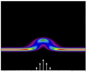
The organization of the paper is as follows. In § 2.1, we pose the mathematical problem, and in § 2.2, we describe the method of solution to compute both eigenvalues and eigenfunctions of the associated non-self-adjoint operator. This allows us to compute solutions given general initial conditions that are valid for any  $t>0$. In § 3, we analyse the behaviour of solutions, focusing first on scale-dependent scalar decay in the case where the initial condition is characterized by a single along-stream mode, and then on the time-varying shear dispersion properties of a localized tracer patch as depicted in figure 1(a,b), respectively. In § 4, we discuss advantages over other methods, as well as the ability to expand our analysis to more complex flows and boundary conditions, and in § 5, we summarize results and future directions.
The two initial conditions considered in this study. (a) A single along-stream mode, with arbitrary cross-stream initial structure. (b) A localized concentration patch centred at  $x=0$. Both types of initial condition are related due to the linearity of the governing equations. Note that the Gaussian function $\varPhi (y)$ is centred at $y={\rm \pi}$ in both cases, although it is not a requirement for our analysis. The domain is identical in both cases.
2. Analytical solutions
2.1. Problem statement
Consider the governing equation (1.1) over a time interval  $t$ in which the velocity field (1.2) is a parallel shear flow of arbitrary amplitude $U_0$, say $\boldsymbol {u}(\boldsymbol {x}, t) = U_0(U(y), 0)$, in a doubly periodic domain defined as $(-L/2\leq x\leq L/2)\times (0\leq y \leq M)$, with $L\geq M$.
We introduce the non-dimensionalization
 \begin{equation} (x, y) = \left[\frac{M}{2{\rm \pi}}\right](x^*, y^*),\quad \boldsymbol{u}= [U_{0}]\boldsymbol{u}^*,\quad t = \left[t_{d}\right]t^*, \end{equation}
where we choose  $M$ as the single length scale, and time is non-dimensionalized by the diffusive time scale $t_{d}=M^2/(4{\rm \pi} ^2\kappa )$. As a result, the non-dimensional governing equation (1.1) becomes (dropping the stars so that from now on we assume all variables are normalized)
 \begin{equation} \frac{\partial\theta}{\partial t} + {\textit{Pe}}\, U(y)\,\frac{\partial\theta}{\partial x} =\nabla^2\theta . \end{equation}
This equation has been studied extensively for a wide range of shear flows (see Eckart Reference Eckart1948; Young et al. Reference Young, Rhines and Garrett1982; Majda & Kramer Reference Majda and Kramer1999; Vanneste Reference Vanneste2006; Camassa, McLaughlin & Viotti Reference Camassa, McLaughlin and Viotti2010). The Péclet number  ${\textit {Pe}}$ is
 \begin{equation} {\textit{Pe}} = \frac{U_{0}M}{2{\rm \pi} \kappa}, \end{equation}
and can be interpreted as the ratio of advective to diffusive time scales ( $2{\rm \pi} U_0t_d /M$) (Rhines & Young Reference Rhines and Young1983). It represents the relative importance of the advective to diffusive tracer fluxes, so a large Péclet number implies weakly diffusive flows. We consider ${\textit {Pe}}$ an arbitrary parameter that can take any value, and implicitly this allows $U_0$ to be time-dependent (since $U_0$ can be considered piecewise constant) when acting on a Fourier tracer mode. Note that both $t_{d}$ and ${\textit {Pe}}$ are domain-scale quantities, independent of the scale of the shear flow, as both are defined with $M$ as opposed to the intrinsic length scale of the flow.
Our choice of a single length scale  $M$ in (2.1a–c) implies the (non-dimensional) doubly periodic boundary conditions
 \begin{equation} \theta(k_mx -{\rm \pi}, y, t) = \theta(k_mx + {\rm \pi}, y, t),\quad \theta(x, y+2{\rm \pi}, t)=\theta(x, y, t), \end{equation}
where  $k_m = M / L$ determines the aspect ratio of the gravest mode that fills the domain (i.e. when $k_m=1$, the domain is a square). The value of $k_m$ is arbitrary and can be made sufficiently small so that the domain approximates a semi-infinite rectangular domain. Our domain choice further implies that any Fourier decomposition in the cross-stream direction is quantized (i.e. individual modes are $l=0, \pm 1, \pm 2, \ldots$), while in the streamwise direction $k=jk_m$, with $j=0, \pm 1, \pm 2, \ldots .$
In general, we are interested in initial conditions that can be expressed via Fourier decomposition as
 \begin{equation} \theta(x, y, 0) = \sum_{i}f_{i}(x)\,\varPhi_{i}(y), \end{equation}
where each of  $f_i(x)$ and $\varPhi _{i}(y)$ are integrable functions in the space of $2{\rm \pi}$-periodic functions.
We consider shear flows defined by an even Fourier series of the form
 \begin{equation} U(y) = \frac{\alpha_{0}}{2}+\sum_{m=1}^{\infty}\alpha_{m} \cos(my) . \end{equation}
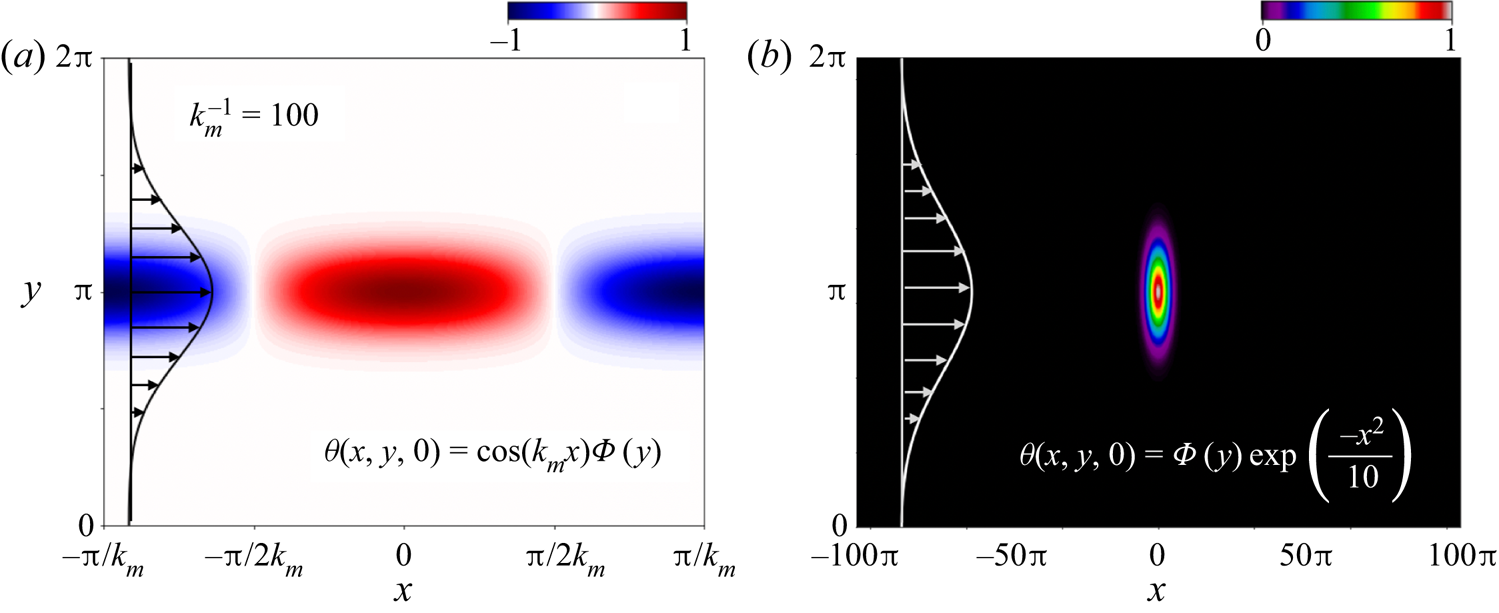
 We introduce an inverse width parameter  $L_d$ that controls the width of a shear flow while keeping intact the shear topology – for example, piecewise constant and piecewise linear shear flows (see figures 2(a,b), also Appendix A). Some of the shear flows considered here are idealized in their velocity gradient, e.g. piecewise constant or concentrated shear. These features represent some aspects of environmental flows whose spatial structure is sensitive to sampling, domain size and background noise. That is, in practice, real flows are patchy, localized and irregular in both time and space. Hence our approach can compute solutions for flows with a discrete, wide spectrum (i.e. $\alpha _m\neq 0$ for arbitrary $m>0$), a feature with theoretical and practical advantages.
Shear flows  $U(y)$, specifically, the (a) triangular, (b) square, (c) Gaussian and (d) polynomial shear flows. The flow widths decrease as $L_d$ increases, and as $L_d \rightarrow \infty$, the shear flows all converge to the same flow, namely, $U=1$ at $y={\rm \pi}$, $U=0$ everywhere else. (e–h) Triangular and square shear flows, as in (a,b), except they have higher $y$-periodicity $P$ (repeated extrema). See Appendix A for the analytic definitions of the shear flow profiles.
An important global property of some shear flows is a symmetry after a translation in  $y$ and reflection in flow amplitude, i.e. a shift–reflect symmetry, defined mathematically as
 \begin{equation} U^*(y-{\rm \pi}/P) ={-} U^*(y), \end{equation}
where  $U^*=U-\alpha _{0}/2$ is the streamline velocity minus its spatial average, and $P=1, 3, \ldots$ is the periodicity of the shear flow maxima within the finite domain (see figure 2). A shear flow that is shift–reflect symmetric has a Fourier series such that
 \begin{equation} U^*(y) = \sum_{m=1}^{\infty}\alpha_{P(2m-1)}\cos[P(2m-1)y] . \end{equation}
For example, the simplest case of a shift–reflect symmetric flow is  $U^*= -(1/2)\cos (y)$. We emphasize that this is a global (domain-scale) property of the flow, independent of ${\textit {Pe}}$, scale and topology of the velocity gradient, and therefore can describe properties of tracer evolution beyond oft-isolated streamlines where shear vanishes.
2.2. Method of solution
Following Camassa et al. (Reference Camassa, McLaughlin and Viotti2010), we take advantage of the linearity of the governing equation (2.2) and the fact that the advection term is  $x$-independent, and consider a separable initial condition for each mode $k$ in the streamwise direction of the form
 \begin{equation} \theta(x, \tilde{y}, t) = \mbox{Re}\left\{\sum_{n=0}^{\infty}\chi_{2n}\, \phi_{2n}( \tilde{y})\exp\left[{\rm i}kx -\omega_{2n}t \right] \right\}, \end{equation}
where  $2\tilde {y}=y$ is a scaled coordinate, $\phi _{2n}(\tilde {y})$ are eigenfunctions, and $\omega _{2n}$ are the associated eigenfrequencies. The coefficients to be determined, $\chi _{2n}$, ensure that the solution satisfies the initial condition (2.5). Substituting (2.9) into (2.2) shows that each eigenfunction satisfies the eigenvalue equation
 \begin{equation} \frac{{\rm d}^2\phi_{2n}}{{\rm d}\tilde{y}^2} + \left[a_{2n} -2q\,U^*(2\tilde{y})\right]\phi_{2n} = 0. \end{equation}
Notice that (2.10) is written with the scaled independent variable  $\tilde {y}=y/2$ to adhere to convention, as it is a type of Hill's equation (see chapter 5 of Magnus & Winkler (Reference Magnus and Winkler2013); also Strutt Reference Strutt1948). When the velocity is the zero-mean, non-normalized cosine shear flow, i.e. $U(2\tilde {y})=\cos (2\tilde {y})$, (2.10) becomes the canonical Mathieu equation (McLachlan Reference McLachlan1947; Olver et al. Reference Olver, Lozier, Boisvert and Clark2010).
Equation (2.10) is an eigenvalue problem that depends on the compound, multiscale parameter
 \begin{equation} q=2{\rm i}k\,{\textit{Pe}}. \end{equation}
This parameter contains the relevant physics of the system, and controls the multiscale, spatial and temporal behaviour of the solutions. From the eigenvalue  $a_{2n}(q)$, the dispersion relation associated with each eigenfunction is given by
 \begin{equation} \omega_{2n} = \frac{a_{2n}(q) +\alpha_{0}q}{4} + k^2. \end{equation}
The term  $k^2$ represents pure diffusion of a normal mode in the $x$-direction, and the eigenvalue $a_{2n}(q)$, which encodes the effect of varying shear in the $y$-direction at that scale, determines the relative contribution of the eigenfunction $\phi _{2n}$ to the tracer evolution in the $y$-direction. The eigenpair $\{a_{2n}, \phi _{2n}\}$ encodes the effect of shear in the tracer evolution in the cross-stream direction at the scale $k^{-1}$.
To calculate the eigenfunctions, we first follow a standard approach when solving Hill's equation (see, for example, chapter VI of McLachlan (Reference McLachlan1947), or Olver et al. Reference Olver, Lozier, Boisvert and Clark2010). Consider an eigensolution of (2.10) of the form
 \begin{equation} \phi_{2n} = \exp(\mu \tilde{y})\sum_{r={-}\infty}^{\infty}C^{(2n)}_{2r}\exp(2r{\rm i}\tilde{y}), \end{equation}
where  $\mu$ is the Floquet exponent, and $\exp (\mu \tilde {y})$ is the Floquet multiplier. In general, all of $\mu$, $a_{2n}$ and $C_{2r}^{(2n)}$ need to be determined (McLachlan Reference McLachlan1947; Magnus & Winkler Reference Magnus and Winkler2013). However, we restrict our analysis to ${\rm \pi}$-periodic solutions in $\tilde{y}$ in order to satisfy (2.4),
and, thus, set
$\tilde{y}$ in order to satisfy (2.4),
and, thus, set  $\mu \equiv 0$ (a different value of $\mu$ results in quasi-periodic solutions). Writing the cosine Fourier series in (2.6) as a sum of complex exponentials (with the property $\alpha _{-m}=\alpha _{m}$), and substituting (2.13) into (2.10), yields the equation
 \begin{align}
& \sum_{r={-}\infty}^{\infty} C^{(2n)}_{2r} \left(
\left[(2r{\rm i})^2 + a_{2n} \right]
\exp(2r{\rm i}\tilde{y})
\right.\nonumber\\
&\quad -q \left[\alpha_{1}
\left\{
\exp[2(r+1){\rm i}\tilde{y}]+
\exp[2(r-1){\rm i}\tilde{y}] \right\}
\right.\nonumber\\
&\quad +\alpha_{2}
\left\{
\exp[2(r+2){\rm i}\tilde{y}] +
\exp[2(r-2){\rm i}\tilde{y}] \right\} \nonumber\\
&\quad +\left.\vphantom{\left[(2r{\rm i})^2 + a_{2n}
\right]}\left.\alpha_{3}
\left\{
\exp[2(r+3){\rm i}\tilde{y}]+
\exp[2(r-3){\rm i}\tilde{y}] \right\}+
\cdots\right]\right) = 0.
\end{align}
\begin{align}
& \sum_{r={-}\infty}^{\infty} C^{(2n)}_{2r} \left(
\left[(2r{\rm i})^2 + a_{2n} \right]
\exp(2r{\rm i}\tilde{y})
\right.\nonumber\\
&\quad -q \left[\alpha_{1}
\left\{
\exp[2(r+1){\rm i}\tilde{y}]+
\exp[2(r-1){\rm i}\tilde{y}] \right\}
\right.\nonumber\\
&\quad +\alpha_{2}
\left\{
\exp[2(r+2){\rm i}\tilde{y}] +
\exp[2(r-2){\rm i}\tilde{y}] \right\} \nonumber\\
&\quad +\left.\vphantom{\left[(2r{\rm i})^2 + a_{2n}
\right]}\left.\alpha_{3}
\left\{
\exp[2(r+3){\rm i}\tilde{y}]+
\exp[2(r-3){\rm i}\tilde{y}] \right\}+
\cdots\right]\right) = 0.
\end{align}
Iterating over all possible values of  $r$ and equating to zero the coefficients multiplying each exponential of arbitrary order $R \in r$, we get the $R$-coefficient recursive equation
 \begin{equation} \left[ \left(2R{\rm i} \right)^2 + a_{2n} \right] C^{(2n)}_{2R}=q \sum_{m={-}\infty}^{\infty}\alpha_{m}C^{(2n)}_{2(R+m)}, \end{equation}
where the  $m=0$ term is not included in the sum on the right-hand side as $\alpha _{0}$ is already incorporated in the eigenvalue via (2.12). Equation (2.15) is almost identical to that studied by Hill in the lunar perigee problem (Hill Reference Hill1886; McLachlan Reference McLachlan1947).
Now split into even and odd  ${\rm \pi}$-periodic eigenfunctions. We define even eigenfunctions as
 \begin{equation} \phi_{2n}^{e}(q, \tilde{y})=\sum_{r=0}^{\infty}A_{2r}^{(2n)}(q)\cos(2r\tilde{y}), \end{equation}
with  $A^{(2n)}_{0}=C^{(2n)}_{0}$ and $A_{2r}^{(2n)}=2C_{2r}^{(2n)}$, $r=\pm 1, \pm 2, \ldots$. These eigenfunctions belong to a class of cosine elliptic functions given their dependence on an eccentricity parameter $q$, and when $q=0$, the eigenfunctions reduce to multiples of $\cos (ny)$ (McLachlan Reference McLachlan1947; Arscott Reference Arscott2014).
Similar to the approach by Chaos-Cador & Ley-Koo (Reference Chaos-Cador and Ley-Koo2002), we cast the bi-infinite recursive equations (2.15) in matrix form as
 \begin{equation} \boldsymbol{T}^{e}\boldsymbol{{X}}_{2n}^e = a_{2n}\boldsymbol{{X}}_{2n}^e , \end{equation}
where the eigenvectors are
 \begin{equation} \boldsymbol{{X}}_{2n}^e = \left[\sqrt{2}A_{0}^{(2n)}, A_{2}^{(2n)}, \ldots, A_{2R}^{(2n)}, \ldots \right]^{{\rm T}}, \end{equation}
and the superscript  $T$ implies transpose. Note that the elements of the eigenvector $\boldsymbol {{X}}_{2n}^e$ are the Fourier coefficients $A_{2r}^{(2n)}$ in (2.16). The vector satisfies an indefinite norm (as in the case of Mathieu's equation; see Brimacombe, Corless & Zamir Reference Brimacombe, Corless and Zamir2021) given by
 \begin{equation} 2\left[A_{0}^{(2n)} \right]^2 + \sum_{r=1}^{\infty}\left[A_{2r}^{(2n)}\right]^2=1, \end{equation}
and a further orthonormality relationship between the Fourier coefficients (Seeger Reference Seeger1997; Ziener et al. Reference Ziener, Rückl, Kampf, Bauer and Schlemmer2012)
 \begin{equation} \sum_{n=0}^{\infty}A_{2r}^{(2n)}A_{2r'}^{(2n)} = \delta_{rr'} - \frac{\delta_{0r}\delta_{0r'}}{2} \quad \text{for}\ r, r' = 0, 1, 2,\ldots, \end{equation}
with Kronecker delta  $\delta _{rr'}$. The bi-infinite matrix $\boldsymbol {T}^e$ associated with (2.16) is
 \begin{gather} \boldsymbol{T}^e =
\begin{bmatrix} 0 & \sqrt{2}q\alpha_{1} &
\sqrt{2}q\alpha_{2} & \cdots & \sqrt{2}q\alpha_{R} &
\cdot\\ \sqrt{2}q\alpha_{1} &
4+q\alpha_{2} & q(\alpha_{1}+\alpha_{3}) & \cdots &
q(\alpha_{R-1}+\alpha_{R+1}) &
\cdot\\ \sqrt{2}q\alpha_{2} &
q(\alpha_{1}+\alpha_{3}) & 16+q\alpha_{4} &
\cdot & \cdot &
\cdot\\ \sqrt{2}q\alpha_{3} &
q(\alpha_{2}+\alpha_{4}) & q(\alpha_{1}+\alpha_{5}) &
\ddots\;\;\;\;\;\;\;\;\;\;\;\;\;\;\; &
\cdot & \cdot\\ \vdots &
\vdots & \;\;\;\;\;\;\;\;\ddots & \;\;\;\;\;\;\ddots &
\vdots & \cdot \\ \vdots & \vdots &
\;\;\;\;\;\;\;\;\;\;\;\ddots &
\;\;\;\;\;\;\;\;\;\;\;\;\;\;\;\;\;\;\;\;\;\;\;\;\;\;\;\ddots
& q(\alpha_{1}+\alpha_{2R-1}) & \cdot \\ \sqrt{2}q\alpha_{R} &
q(\alpha_{R-1}+\alpha_{R+1}) & \cdots &
q(\alpha_{1}+\alpha_{2R-1}) & 4R^2 +q\alpha_{2R} &
\cdot\\
\cdot & \cdot
& \cdot &
\cdot & \cdot
& \cdot \end{bmatrix}.
\end{gather}
\begin{gather} \boldsymbol{T}^e =
\begin{bmatrix} 0 & \sqrt{2}q\alpha_{1} &
\sqrt{2}q\alpha_{2} & \cdots & \sqrt{2}q\alpha_{R} &
\cdot\\ \sqrt{2}q\alpha_{1} &
4+q\alpha_{2} & q(\alpha_{1}+\alpha_{3}) & \cdots &
q(\alpha_{R-1}+\alpha_{R+1}) &
\cdot\\ \sqrt{2}q\alpha_{2} &
q(\alpha_{1}+\alpha_{3}) & 16+q\alpha_{4} &
\cdot & \cdot &
\cdot\\ \sqrt{2}q\alpha_{3} &
q(\alpha_{2}+\alpha_{4}) & q(\alpha_{1}+\alpha_{5}) &
\ddots\;\;\;\;\;\;\;\;\;\;\;\;\;\;\; &
\cdot & \cdot\\ \vdots &
\vdots & \;\;\;\;\;\;\;\;\ddots & \;\;\;\;\;\;\ddots &
\vdots & \cdot \\ \vdots & \vdots &
\;\;\;\;\;\;\;\;\;\;\;\ddots &
\;\;\;\;\;\;\;\;\;\;\;\;\;\;\;\;\;\;\;\;\;\;\;\;\;\;\;\ddots
& q(\alpha_{1}+\alpha_{2R-1}) & \cdot \\ \sqrt{2}q\alpha_{R} &
q(\alpha_{R-1}+\alpha_{R+1}) & \cdots &
q(\alpha_{1}+\alpha_{2R-1}) & 4R^2 +q\alpha_{2R} &
\cdot\\
\cdot & \cdot
& \cdot &
\cdot & \cdot
& \cdot \end{bmatrix}.
\end{gather} Odd eigenfunctions satisfy the same equation as in (2.10), but the nomenclature changes, with  $b_{2n+2}(q)$ now indicating the odd eigenvalue (see Arscott Reference Arscott2014). The odd (sine elliptic) eigenfunctions are defined as
 \begin{equation} \phi^o_{2n+2}(q, \tilde{y}) = \sum_{r=0}^{\infty}B_{2r+2}^{(2n+2)}\sin\left[(2r+2)\tilde{y}\right]. \end{equation}
When  $q=0$, these eigenfunctions reduce to multiples of $\sin [(n+1)y]$. The coefficients satisfy the normalization under an indefinite norm
 \begin{equation} \sum_{r=0}^{\infty}\left[B_{2r+2}^{(2n+2)}\right]^2 = 1, \end{equation}
and the orthonormalization
 \begin{equation} \sum_{n=0}^{\infty}B_{2r+2}^{(2n+2)}B_{2r'+2}^{(2n+2)} = \delta_{rr'},\quad \text{for}\ r, r' = 0, 1, 2,\ldots. \end{equation}
Similar to (2.17), the matrix equation for the odd eigenfunction–eigenvalue pair is
 \begin{equation} \boldsymbol{T}^{o}\boldsymbol{{X}}_{2n+2}^o = b_{2n+2}\boldsymbol{{X}}_{2n+2}^o, \end{equation}
where
 \begin{equation} \boldsymbol{X}_{2n+2}^o = \left[B_{2}^{(2n+2)}, B_{4}^{(2n+2)}, \ldots, B_{2R+2}^{(2n+2)}, \ldots \right]^{{\rm T}}. \end{equation}
The odd bi-infinite matrix is
 \begin{gather} \boldsymbol{T}^o =
\begin{bmatrix}4-q\alpha_{2} & q(\alpha_{1}-\alpha_{3}) &
q(\alpha_{2}-\alpha_{4}) & \cdots &
\cdot &
\cdot\\ q(\alpha_{1}-\alpha_{3}) &
16-q\alpha_{4} & q(\alpha_{1}-\alpha_{5}) & \cdots &
\cdot &
\cdot\\ q(\alpha_{2}-\alpha_{4}) &
q(\alpha_{1}-\alpha_{5}) & 36-q\alpha_{6} & \cdots &
\cdot &
\cdot\\ \vdots & \vdots & \vdots &
\ddots & q(\alpha_{1}-\alpha_{2R-1}) & \cdot \\ q(\alpha_{R-1}-\alpha_{R+1}) & \cdots &
\cdots & q(\alpha_{1}-\alpha_{2R-1}) & 4R^2 -q\alpha_{2R} &
\cdot\\
\cdot & \cdot
& \cdot &
\cdot & \cdot
& \cdot \end{bmatrix} .
\end{gather}
\begin{gather} \boldsymbol{T}^o =
\begin{bmatrix}4-q\alpha_{2} & q(\alpha_{1}-\alpha_{3}) &
q(\alpha_{2}-\alpha_{4}) & \cdots &
\cdot &
\cdot\\ q(\alpha_{1}-\alpha_{3}) &
16-q\alpha_{4} & q(\alpha_{1}-\alpha_{5}) & \cdots &
\cdot &
\cdot\\ q(\alpha_{2}-\alpha_{4}) &
q(\alpha_{1}-\alpha_{5}) & 36-q\alpha_{6} & \cdots &
\cdot &
\cdot\\ \vdots & \vdots & \vdots &
\ddots & q(\alpha_{1}-\alpha_{2R-1}) & \cdot \\ q(\alpha_{R-1}-\alpha_{R+1}) & \cdots &
\cdots & q(\alpha_{1}-\alpha_{2R-1}) & 4R^2 -q\alpha_{2R} &
\cdot\\
\cdot & \cdot
& \cdot &
\cdot & \cdot
& \cdot \end{bmatrix} .
\end{gather} From matrices (2.21) and (2.27), the eigenvalue–eigenfunction pairs  $\{a_{2n}(q), \boldsymbol {X}^e_{2n}(q)\}$ and $\{b_{2n+2}(q), \boldsymbol {X}^o_{2n+2}(q)\}$ are determined, and with them the associated eigenfunctions $\phi ^{e}_{2n}(q, \tilde {y})$ and $\phi ^o_{2n+2}(q, \tilde {y})$ are found via (2.16) and (2.22). Moreover, the orthonormality relations (2.19)–(2.20) and (2.23)–(2.24) imply that the eigenfunctions $\phi ^{e}_{2n}$ and $\phi ^o_{2n+2}$ are orthonormal. That is, for any value of $q=2{\rm i}k\,{\textit {Pe}}$, each eigenfunction satisfies
 \begin{equation} \int_{0}^{\rm \pi}\phi_{2n'}^e(q, \tilde{y})\,\phi^e_{2n}(q, \tilde{y})\,{\rm d}\tilde{y} = \frac{{\rm \pi}\delta_{nn'}}{2},\quad \text{for}\ n,n'=0, 1, 2,\ldots . \end{equation}
Similarly, the odd eigenfunctions satisfy
 \begin{equation} \int_{0}^{\rm \pi}\phi_{2n'+2}^o(q, \tilde{y})\,\phi^o_{2n+2}(q, \tilde{y})\,{\rm d}\tilde{y} = \frac{{\rm \pi}\delta_{nn'}}{2},\quad \text{for}\ n,n'=0, 1, 2,\ldots . \end{equation}
Finally, using (2.16) and (2.22), and the orthogonality of normal modes, we get the following transformation (i.e. a change in basis):
 \begin{equation} \sum_{n=0}^{\infty}(1+\delta_{r0})\,A_{2r}^{(2n)}(q)\,\phi_{2n}^e(q, \tilde{y}) = \cos(2r\tilde{y}),\quad r =0, 1, 2, \ldots, \end{equation}
and
 \begin{equation} \sum_{n=0}^{\infty}B_{2r+2}^{(2n+2)}(q)\,\phi^o_{2n+2}(q, \tilde{y}) = \sin[(2r+2)\tilde{y}],\quad r =0, 1, 2, \ldots . \end{equation}
 The derivations above imply that the non-self-adjoint nature of the advection–diffusion operator (2.2) is captured by the properties of the matrices (2.21) and (2.27), determined by their dependence on  $q=2{\rm i}k\,{\textit {Pe}}$, and by the shear (through $\alpha _m\neq 0$, $m=1, 2, \ldots$). As $q$ is imaginary, the matrices are Hermitian only in the absence of shear ( $\alpha _m\equiv 0$ for all $m=1, 2, 3,\ldots$), or when $q\equiv 0$ ( $k=0$ or ${\textit {Pe}}=0$). In those cases, the advection–diffusion operator is self-adjoint.
In the presence of shear, the bi-infinite matrices  $\boldsymbol {T}^e$ and $\boldsymbol {T}^o$ belong to a wide class of non-self-adjoint operators associated with $\mathcal {PT}$-symmetric Hamiltonians (Bender & Boettcher Reference Bender and Boettcher1998; Bender Reference Bender1999; Heiss Reference Heiss2004, Reference Heiss2012). A characteristic of these systems, beyond their dependence on a single parameter (here $q$), is the analytical coalescing of eigenvalues in their real parts at isolated, discrete values of the parameter $q=q_{EP}$ called exceptional points (EPs). At EPs, the imaginary parts of the eigenvalues branch, to create complex-conjugate eigenvalue pairs for $q>q_{EP}$ (Hunter & Guerrieri Reference Hunter and Guerrieri1981; Hernández & Mondragón Reference Hernández and Mondragón1994; Heiss Reference Heiss1999, Reference Heiss2004; Miri & Alu Reference Miri and Alu2019). EPs are anticipated for all the eigenvalues for shear flows that are shift–reflect symmetric. The reason is that in such flows, the diagonal elements of $\boldsymbol {T}^e$ and $\boldsymbol {T}^o$ are real, so their eigenvalues are either real or occur in complex-conjugate pairs (see figures 3a,b).
(a,c,e) Real and (b,d,f) imaginary shifted eigenvalues  $a_{2n}+\alpha _{0}q$ associated with the (a–b) square and (c–f) Gaussian shear flows of different widths (see figure 2c). Light grey lines correspond to eigenvalues with negative imaginary parts ( $\mbox {Im}\{a_{2n}\}<0$), so the shifted imaginary values lie below the dashed grey line $\alpha _{0}q$. Black lines correspond to eigenvalues with positive imaginary parts ( $\mbox {Im}\{a_{2n}\}>0)$. In the limit $k\,{\textit {Pe}} \rightarrow 0$, all eigenvalues converge to $a_{2n}\rightarrow 4n^2$, $n=0, 1, 2,\ldots.$ Only the gravest 40 eigenvalues are plotted.

At EPs, the eigenfunctions coalesce too, resulting in a gap in the completeness of the set of eigenfunctions. This implies the need to supplement the set of eigenfunctions (Brimacombe et al. Reference Brimacombe, Corless and Zamir2021). Because EPs are isolated discrete points (e.g. the first EP in Mathieu's equation is  $q_{EP}=1.468768613785142{\rm i}$, per Brimacombe et al. Reference Brimacombe, Corless and Zamir2021), however, it is extremely rare to match an EP exactly with a generic combination of $k$ and ${\textit {Pe}}$. In the rare case of an exact match, perturbing $k$ or ${\textit {Pe}}$ avoids evaluating at the EP location in $q$-space. In practice, the ability to compute the eigenvalue spectra a priori allows for the inspection for EPs. If they occur, then appropriate changes to $k$ or ${\textit {Pe}}$ can be made. Hence, there is no practical need to supplement the set of eigenfunctions, and for the rest of paper, we avoid explicit evaluation at EPs when computing analytical solutions.
Changing the periodicity of the shear flow by increasing the value of  $P$ (e.g. from $P=1$ to $P=2$ as seen in figures 2a,e) introduces multiple extrema in the shear flow profile that are shifted by $2{\rm \pi} /P$ in $y$. If the shear flow was previously shift–reflect symmetric, then the EPs of the resulting $P$-periodic shear flows can involve multiple eigenvalues and mergers that are more complex than the coalescence of a complex-conjugate pair.
The non-self-adjoint character of the linear operator (2.2) imprints on the spatial (via eigenfunctions) and temporal (via eigenvalues) behaviour of solutions. To illustrate this point, we focus on the pair  $\{a_{2n}, \phi _{2n}^e\}$ associated with shear flows that are shift–reflect symmetric; such flows represent a special case in which eigenvalues are dense with EPs. When evaluated at $q$ values beyond an EP, the eigenfunctions $\{\phi ^e_{2n}\}$ associated with complex conjugated eigenvalues that have coalesced satisfy their own shift–reflect symmetry (see Appendix B; also Ziener et al. Reference Ziener, Rückl, Kampf, Bauer and Schlemmer2012). That is, the two symmetric eigenfunctions describe identical spatial behaviour in the solution that are shifted from one another in space by $\tilde {y}={\rm \pi} /2$ ( $y={\rm \pi}$). Given that the complex-conjugate eigenvalue pair describes equal eigenfunction decay rates (determined by $\mbox {Re}\{a_{2n}\}$) and opposite directions of eigenfunction propagation (determined by $\mbox {Im}\{a_{2n}\}$), the tracer evolution in the subdomain characterized by $U^*<0$ is an exact mirror image of the tracer evolution in the subdomain characterized by $U^*>0$. This means that a priori knowledge of the Fourier series of a shear flow that is shift–reflect symmetric provides a deep fundamental understanding of a global property of the tracer distribution at all times.
The present method of solution relies on the convergence of the spectra of the truncated eigenvalue systems (2.17) and (2.25) with respect to the original non-truncated bi-infinite system (see Ikebe et al. Reference Ikebe, Asai, Miyazaki and Cai1996; Deconinck & Kutz Reference Deconinck and Kutz2006; Curtis & Deconinck Reference Curtis and Deconinck2010). The convergent truncation implies that there is a large enough matrix size  $(R+1)\times (R+1)$ for which the eigenvalue–eigenfunction pairs calculated are sufficiently accurate. It also implies that higher cross-stream modes (in $y$) can be approximated by
 \begin{equation} a_{2n'} = (2n')^2,\quad \phi^e_{2n'} = \cos(2n'\tilde{y}) ,\quad n'>R+1, \end{equation}
and
 \begin{equation} b_{2n'+2} = (2n'+2)^2,\quad \phi^o_{2n'+2} = \sin[(2n'+2)\tilde{y}],\quad n'>R. \end{equation}
 Following Ziener et al. (Reference Ziener, Rückl, Kampf, Bauer and Schlemmer2012), an accurate truncation is one that ensures that the orthogonality relations (2.20)–(2.24) are satisfied. A first-order guess for a truncated size  $R$ comes from ensuring that the truncated matrix is always diagonally dominant. Given that the diagonal term is $4R^2\pm q\alpha _{2R}$, and $|\alpha _{2R}|\rightarrow 0$ for increasing $R$, a truncation size can be estimated from the ratio between the diagonal terms and the super-diagonal terms. This is
 \begin{equation} 4R^2 \gg |q|\max{|\alpha_m|}. \end{equation}
(This condition implies absolute and uniform convergence of the trigonometric series (2.16); Arscott Reference Arscott2014.)
Since the truncated matrix size  $R$ depends explicitly on ${\textit {Pe}}$ via $|q|=2k\,{\textit {Pe}}$, the truncated matrices $\boldsymbol {T}^e(q)$ and $\boldsymbol {T}^o(q)$ grow in size like ${\textit {Pe}}^{1/2}$. For this reason, the present eigenvalue approach to solve the governing equation (2.2) is most efficient at intermediate and low ${\textit {Pe}}$ values (i.e. ${\textit {Pe}} < 10^{4}$), although there is no restriction on how large ${\textit {Pe}}$ can be.
The value of  $R$ further quantifies the cross-stream cutoff wavenumber $l_c$, past which small scales become only weakly influenced by the presence of shear, and higher modes in an arbitrary initial condition decay as pure diffusion. From (2.34), we define this scale as
 \begin{equation} l_{c} = G\sqrt{|\alpha_{max}|\,k\,{\textit{Pe}} / 2}, \end{equation}
where  $G\gg 1$ is an arbitrary constant. (A value in the range $G^2 \geq 50$ already yields good results.)
The approximations (2.32a,b)–(2.32a,b) expose the multiscale nature of scalar mixing in the cross-stream direction, i.e. they reflect a pure diffusive behaviour at high enough cross-stream wavenumbers for every streamwise (Fourier mode)  $k$. In this sense, the cross-stream scale $l_c$ complements the estimate of streamwise scale at which variance decays diffusively in the cosine shear flow (Camassa et al. Reference Camassa, McLaughlin and Viotti2010).
2.3. General solution
Without loss of generality, we now consider an initial condition that consists of a single term in the sum in (2.5), determined by  $f(x)$ and $\varPhi (2\tilde {y})$, functions that are expressed via the Fourier series
 \begin{equation} f(x) = \sum_{j=0}^{\infty}c_{j}\cos(\,j k_m x) \end{equation}
and
 \begin{equation} \varPhi(2\tilde{y}) = \sum_{l=0}^{\infty}\chi^e_{l}\cos(2l\tilde{y}) + \chi^o_{l}\sin(2l\tilde{y}) , \end{equation}
where  $c_{j}$, $\chi ^e_{l}$ and $\chi ^o_{l}$ are coefficients determined by inversion formulas from known $f(x)$ and $\varPhi (2 \tilde {y})$, with $j,l=0, 1, 2,\ldots.$ Using (2.30)–(2.31), we write the cross-stream initial condition (2.37) in terms of the new eigenbasis as
 \begin{equation} \varPhi(2\tilde{y}) = \sum_{n,l=0}^{\infty} \chi^{*}_{l}\,A_{2l}^{(2n)}(q)\, \phi^e_{2n} + \chi^o_{l}B_{2l+2}^{(2n+2)}\phi^o_{2n+2}, \end{equation}
where  $\chi _l^* = (1+\delta _{l0})\chi _l^e$. Then the general solution to (2.2) associated with an initial condition (2.5) and doubly periodic boundary conditions is given by the triple sum
 \begin{align} \theta(x, \tilde{y}, t) &= \mbox{Re}\left\{\sum_{j, n, l=0}^{\infty} c_{j}\left[\chi_{l}^{*}A_{2l}^{(2n)} \phi_{2n}^e \exp\left(-\frac{a_{2n}}{4}t\right) + \chi^o_{l}B_{2l+2}^{(2n+2)}\phi_{2n+2}^o \exp\left(-\frac{b_{2n+2}}{4}t\right)\right] \right. \nonumber\\ &\quad \left.\vphantom{\sum_{j, n, l=0}^{\infty}} {}\times \exp\left[{\rm i} j k_m\left(x-\frac{\alpha_{0}\,{\textit{Pe}}}{2}\,t \right) - \left((\,j k_m)^2 \right)t \right] \right\}. \end{align}
 The analytical solution (2.39) results from a constant  $U_0$ and thus single ${\textit {Pe}}$ value. In the case of a time-varying amplitude, additional $N$ different $U_0$ values that approximate $U_{0}(t)$ then generate $N$-sets of eigenfunction–eigenvalue pairs, each with a solution expression that looks like that in (2.39). The ability to solve for arbitrary initial conditions via their Fourier coefficients (2.36)–(2.37) allows (2.39) to represent the solution to a time and amplitude varying shear flow during a time interval at which $U_0$ is effectively constant.
3. Results
We now apply these new methods of solution to explore the tracer evolution of two types of initial conditions: (1) a single streamwise Fourier mode (as in figure 1a), for which we characterize the modal decay rate, and relate it to the gravest eigenvalues, confirming and extending the asymptotic analysis of Camassa et al. (Reference Camassa, McLaughlin and Viotti2010); (2) a localized concentration (tracer patch, as in figure 1b), for which we characterize the tracer dispersion via its central moments, extending the particle study of the Poiseuille flow by Latini & Bernoff (Reference Latini and Bernoff2001). Appendix C contains a useful reference to variable names in tabular form, and in Appendix D, we provide a comparison of the analytic solutions to numerical solutions from the open source package Oceananigans (Ramadhan et al. Reference Ramadhan, Wagner, Hill, Campin, Churavy, Besard, Souza, Edelman, Ferrari and Marshall2020), with excellent results.
3.1. Modal solutions
Consider a centred initial condition describing a single streamwise Fourier mode that is localized in the cross-stream direction:
 \begin{equation} \theta(t=0) = \cos(kx)\exp\left[-4\left(y-{\rm \pi}\right)^2 \right]. \end{equation}
The analytical solution with this initial condition is (2.39) for a single mode  $k$ and cross-stream coefficients
 \begin{equation} \chi^*_{l} = \frac{1}{2\sqrt{\rm \pi}}\exp\left(-{\rm i}l{\rm \pi} \right) \exp\left[ -\left(\frac{l}{4} \right)^2\right],\quad l=0, 1, 2,\ldots. \end{equation}
The  $l=0$ term implies the presence of a non-zero cross-stream average, although the global (area average) remains zero. We refer to the initial condition (3.1) as modal and centred, given the absence of odd cross-stream Fourier coefficients ( $\chi _l^{o}\equiv 0$ in (2.38)).
Snapshots of solutions  $\theta$ to (2.2) for a Gaussian shear flow ( $L_d=4/3$) are shown in figure 4. At low $q=4{\rm i}$ (figures 4a–d), the long-term evolution of $\theta$ settles into a domain-scale structure. The solution does not exhibit clearly the two distinct spatially separated behaviours associated with subdomains defined by our choice of $U^*<0$ and $U^*>0$. At larger $q=640{\rm i}$, the solution does exhibit two distinct behaviours (figures 4e–h). Given our choice of flow normalization, tracer variance is homogenized much more rapidly near the peak of the shear flow ( $U^*>0$) than away from it ( $U^*<0$). (The actual sign of $U^*$, which arises from our particular choice of mean velocity, has no direct effect on the decay rate of tracer variance.) The initial condition centred at $y_{0}={\rm \pi}$ facilitates the distinction between the subdomains $U^*>0$ and $U^*<0$ for large enough $q$, although an arbitrary initial condition may not. Such behaviour is associated with the localization of the eigenfunctions within shear-free regions as $q$ becomes large.
Snapshots of modal solutions for two wavenumbers  $k_m$ and two values of canonical parameter $q=2{\rm i}k_m\,{\textit {Pe}}$ at fixed ${\textit {Pe}} = 1000$. The shear flow is Gaussian with inverse width parameter $L_d=4/3$ (black curve in (a) and figure 2c). The streamwise axis is scaled by (domain-scale) wavenumber $k_m$, and the colour scales differ between snapshots.

To quantify the transient and long-term decay of tracer variance, we compute
 \begin{equation} \sigma ={-}\frac{1}{2}\,\frac{{\rm d}\log(\|\theta\|_{2}^{2})}{{\rm d} t}, \end{equation}
where  $\|\theta \|_{2}^{2}$ is the $L_2$-norm defined by
 \begin{equation} \|\theta\|_{2}^{2} (t) = \int_{-{\rm \pi}/k}^{{\rm \pi}/k} \int_{0}^{2{\rm \pi}}\theta^2\,{{\rm d}y}\,{{\rm d}x} . \end{equation}
With initial condition (3.1), we identify two non-overlapping plateaus in the  $\sigma$ time series for sufficiently small streamwise scales, or equivalently, sufficiently large ${\textit {Pe}}$. Each plateau implies that a single eigenvalue–eigenfunction pair dominates the (spatio-temporal) decay rate of tracer variance, with tracer localized to regions where $U^*$ has extrema (see figures 5a–d). We refer to the plateaus as pure modal decay rates, denoted as $\bar {\sigma }$. Varying $k$ at constant ${\textit {Pe}}$ reveals the $q$-dependence of the gravest two eigenvalues, as seen in figure 5(e). These are the (averaged) modal decay rates estimated in Camassa et al. (Reference Camassa, McLaughlin and Viotti2010) in that case for the cosine shear flow. An off-centred initial condition ( $\chi ^o_l\neq 0$) can yield a $\sigma$ time series in which the two plateaus overlap, and distinguishing between the two even eigenvalue–eigenfunction pairs can be unclear.
(a–d) Time series of decay rate  $\sigma (t)$ (black) and variance $\|\theta \|_{2}^{2}$ (blue, normalized by its initial value) for fixed ${\textit {Pe}} = 1000$ and various choices of wavenumber $k$ (hence canonical parameter $q=2{\rm i}k\,{\textit {Pe}}$) in the modal initial condition (3.1). The shear flow is Gaussian ( $L_d=4/3$). The red dots in (b,c) represent the times of the snapshots shown in figures 4(a–d) and 4(e–h), respectively. (e) Pure modal decay rate $\bar {\sigma }$ showing the distinct regimes of scalar decay as a function of streamwise wavenumber $k$. The black and red dots are from analytical solutions, and the blue dots are from numerical simulations. Shown in (e) are the asymptotic curves for the gravest eigenvalues $a_{2}$ (black, at large $q$) and $a_{0}$ (red, at both small and large $q$). Grey arrows connect the distinct $\sigma$ time series in (a–d) with their averaged values in (e). Note that the log-log plot accentuates large and small $k$ behaviour.

Figure 6 shows that the three regimes of scalar decay, described by Camassa et al. (Reference Camassa, McLaughlin and Viotti2010) for the cosine shear flow, are present in all shear flows, and are therefore generic. For arbitrary  ${\textit {Pe}}$, we define these three regimes using a critical canonical parameter $q_{cr}$ as follows. For small $q$ values, $|q|<|q_{cr}|$, the gravest eigenvalue is real (see table 1). Thus at long-enough (streamwise) scales, $|q|< q_{cr}$ and $\bar {\sigma }\propto k^2$, with a coefficient proportional to ${\textit {Pe}}^2$. This is the regime of Taylor dispersion because it describes a diffusion process with effective diffusivity $\kappa ^*$, given dimensionally by
 \begin{equation} \kappa^* = \frac{U_0^2 M^2}{2{\rm \pi}^2\kappa}\sum_{m=1}^{\infty}\frac{\alpha_{m}^2}{2m^2}. \end{equation}
The exact result  $\beta _2=\sum _{m=1}^{\infty }(\alpha _{m}^2/(2m^2))$ is derived in Appendix E, for all shear flows considered here. This expression for the effective diffusivity matches that first derived in Zel'dovich (Reference Zel'dovich1982) for time-oscillatory, periodic shear flows (when considering vanishing frequency; see also Majda & Kramer Reference Majda and Kramer1999; Smith Reference Smith2005; Haynes & Vanneste Reference Haynes and Vanneste2014).
Pure modal decay rate  $\bar {\sigma }$ for all flows considered with single maxima ( $P=1$). The different lines are from analytical predictions of the asymptotic behaviour of the gravest eigenvalues $a_{0}$ and $a_{2}$ at large and small $q$, along with the pure diffusion case $k^2$. In all cases, ${\textit {Pe}}=1000$. For values of the $\beta _2$, $c$ and $s$ coefficients, see table 2.

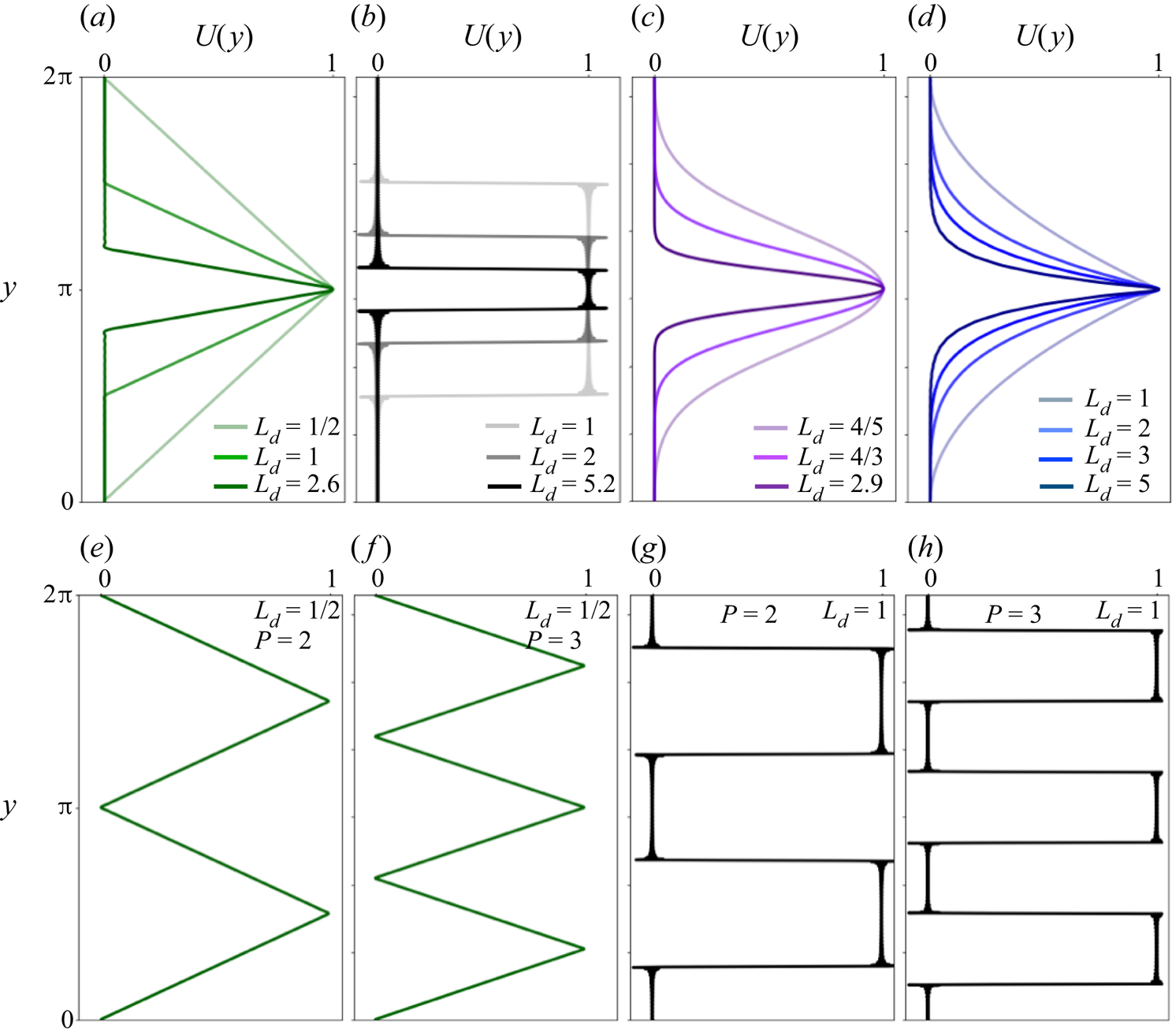
Critical canonical parameters  $|q_{cr}|$ for shear flows considered. The parameter $P$ represents the periodicity of the shear flow within the domain: $P=1$ for a single peak (single maximum), and $P=2$ and $P=3$ imply two and three shear flow maxima (peaks), respectively, as shown in figures 2(e–h).
At intermediate scales,  $k>|q_{cr}|/(2\,{\textit {Pe}})$, the gravest eigenvalue $a_{0}$ becomes complex and the pure modal decay rate is anomalous, meaning $\bar {\sigma }\propto k^s$ with $s<2$. In fact, pure modal decay rates in the $U^*>0$ and $U^*<0$ regions generally separate (see figure 6). Only when the flow is shift–reflect symmetric – as in the cosine, triangular and square shear flows, where eigenvalues appear as complex-conjugate pairs – do we find a single pure modal decay rate to determine the anomalous modal decay for all values of $q$.
$q$.
The algebraic dependence of the gravest eigenvalues at large  $q$ can be derived via a WKB analysis localized to regions with vanishing shear where $U^*$ has an extrema. In other words, the values of $\bar {\sigma }$ in this asymptotic limit depend explicitly on the gradient of shear at the flow extrema, where shear changes sign (e.g. see Hunter & Guerrieri Reference Hunter and Guerrieri1981; Camassa et al. Reference Camassa, McLaughlin and Viotti2010). The eigenvalues take the form
 \begin{equation} a_{2n} \sim d_{1}q^{s} - d_{2}q, \end{equation}
where  $d_{1}$ and $d_{2}$ are coefficients independent of $q$, and the exponent $s<2$ is real. But the asymptotic behaviour (3.6) strictly applies only in the limit $|q|\rightarrow \infty$ where the eigenfunctions are localized to shear-vanishing regions, and remains greatly inaccurate at intermediate $q$ values near $q_{cr}$ (the actual range of validity varies for each shear flow). This severely constrains the applicability of asymptotic (pure) modal decay rates to realistic flows with finite ${\textit {Pe}}$ values, and arbitrary initial conditions. (It is applied successfully in (Camassa et al. Reference Camassa, McLaughlin and Viotti2010) to describe the evolution of a multiscale initial condition that concentrates tracer variance at very large scales and very small scales, well separated in spectral space.) Figures 7(a–c) show this error for the square shear flow in the estimate of pure modal decay rates (red dashed lines) as these get extrapolated towards intermediate $q$ values near $q_{cr}$. The implication is that for arbitrary ${\textit {Pe}}$ values, the asymptotic approach incorrectly predicts faster (pure modal) decay rates of tracer variance, meaning an over-mixing at intermediate scales.
Fits (dashed lines) to the gravest eigenvalues with positive (thick black curves) and negative (thin grey curves) imaginary parts for (a–c) square and (d–f) Gaussian shear flows for various inverse width parameters  $L_d$ (see figure 2).

The asymptotic expression (3.6) provides an accurate approximation of  $\bar {\sigma }$ at large q, and so we use it to estimate the streamwise scale of transition from a regime of anomalous decay into a pure diffusive scalar decay behaviour (Camassa et al. Reference Camassa, McLaughlin and Viotti2010). This represents the (streamwise) scale at which decay of tracer variance of the longest-lived tracer patches becomes insensitive to cross-stream shear. Excluding shift–reflect symmetric flows, two distinct $\bar {\sigma }(k)$ curves exist, so this transition varies across the domain.
At large  $q$ values, the pure modal decay rate takes the form
 \begin{equation} \bar{\sigma}^{{\pm}} \sim c_{{\pm}}\left(k\,{\textit{Pe}} \right)^{s_{{\pm}}}, \end{equation}
where the  $\pm$ signs reflect the positive ( $+$) and negative ( $-$) signs of the imaginary parts of the eigenvalues (and hence the sign of $U^*$). From (3.6), the coefficients connect as
 \begin{equation} c_{{\pm}}=\frac{2^{s_{{\pm}}}d_{1^\pm}}{4}. \end{equation}
From the fitted coefficients  $s_\pm$ and $d_{1^\pm }$, and (3.8), we calculate $c_{\pm }$ values and list them in table 2. Using (3.7), the transition scale $k_d$ into the pure diffusion regime is
 \begin{equation} k_d^{{\pm}} = \left(c_{{\pm}}\,{\textit{Pe}}^{s_{{\pm}}} \right)^{{1}/{(2-s_{{\pm}})}}. \end{equation}
For values  $s_{+}=0.5$ typical for the Gaussian shear flows, $k_d\propto {\textit {Pe}}^{1/3}$, equating that of the cosine shear flow derived previously (see Camassa et al. Reference Camassa, McLaughlin and Viotti2010). From (3.9), we find a strong dependence of ${\textit {Pe}}$ scaling the type of shear (e.g. piecewise linear, continuous, constant) from the computed values of the $s_\pm$ parameter, and therefore a spatial dependence of the ${\textit {Pe}}$ scaling when flows are not shift–reflect symmetric. This means that the rate of tracer variance decays as pure streamwise diffusion over two distinct range of modes if the shear curvature is different in the different shear-vanishing regions. This can be seen clearly in the narrow flows in figures 6(k–m), for which there are two distinct range of (streamwise) scales that decay diffusively.
Parameters that determine the pure modal decay rates  $\bar {\sigma }$ in Taylor's and the anomalous diffusion regimes of shear dispersion. To visualize these values, see figure 6.

Moreover, since (3.9) relies on the accuracy of (3.6), such a transition scale is accurate only under the large- $q$ limit. In our eigenfunction approach, the transition scale for arbitrary ${\textit {Pe}}$ values can be computed directly form the eigenvalues $a_{0}$ and $a_{2}$ calculated from matrices $\boldsymbol {X}^e$ and $\boldsymbol {X}^o$, but the functional dependence on ${\textit {Pe}}$ as expressed in (3.6) is not easily available given the unknown analytical expression $a_{2n}=a_{an}(q)$ at intermediate $q$ values.
The intermediate  $q$ values are also significant in the case of time-varying amplitude, given that varying ${\textit {Pe}}$ is equivalent to varying the amplitude of the shear flow. In that case, the curves $\beta _{2}\,{\textit {Pe}}^2\,k^2$ in figure 6 associated with the small- $q$ limit (Taylor's regime of scalar decay) and those of the anomalous decay shift vertically, although the former regime is much more sensitive to time-amplitude changes due to the ${\textit {Pe}}^2$ dependence. The pure diffusion ( $k^2$) remains insensitive to ${\textit {Pe}}$ values, but the scale of transition $k_d^{\pm }$ into the pure diffusion regime remains sensitive to Pe.
From all the values of  $s_{\pm }$ in table 2, observe the following.
(i) When shear is discontinuous (as in the polynomial and triangular shear flows), $s_{+}\approx 2/3$ independent of the width of the flow $L_d$.
(ii) When shear is continuous, the exponent lies in the range
$0.025 \leq s\leq 0.5$, and the largest exponent is associated with flows whose local curvature is quadratic. The smallest exponent corresponds to the square shear flow. These results are independent of the width of the flow $L_d$.


Observations (i) and (ii) were first shown for the cosine and linear shear flows (Camassa et al. Reference Camassa, McLaughlin and Viotti2010), and we show that these are universal across any shear flow that has an integrable dependence on  $y$, independent of shear flow width. However, as the shear flows narrow ( $L_d$ increases), increasingly large values of $|q|$ are necessary for the eigenvalues to asymptote, according to (3.6). This behaviour leaves an increasingly large range of intermediate $q$ values (hence scales $k$ for arbitrary ${\textit {Pe}}$) for which (3.6) is inaccurate, most obviously for the square shear flow (solid black and dashed red lines in figures 7a–c). This implies an over-mixing estimate within regions of vanishing shear, and under-mixing away from these regions, at intermediate scales. For time and amplitude varying shear flows that continuously reassign Fourier modes onto new $q$ values, such spurious mixing behaviour would only be accentuated. (Any change to the amplitude of a shear flow is equivalent to modifying the ${\textit {Pe}}$ value in our analysis.)
3.2. Time-varying dispersion of a localized concentration
We now consider the time-varying dispersion of a tracer patch defined by the initial condition
 \begin{equation} \theta(x, y, 0) = \exp\left[-\left(\frac{x}{\sqrt{2\mu_{2}(0)}}\right)^2- \left(\frac{y-y_0}{\sqrt{0.02}}\right)^2 \right]. \end{equation}
The initial widths of the patch in the cross-stream and streamwise directions are  $1/100$ and $\mu ^{1/2}_{2}(0)$, respectively. (We define the initial streamwise width using the nomenclature associated with the second central moment in (3.11) at time $t=0$.) A large literature exists on the time evolution of a localized plume in laminar flows, and the enhanced transport that derives from the combined action of differential advection and mixing (i.e. shear dispersion; see Aris Reference Aris1956; Elrick Reference Elrick1962; Lighthill Reference Lighthill1966; Young et al. Reference Young, Rhines and Garrett1982; Rhines & Young Reference Rhines and Young1983; Ferrari et al. Reference Ferrari, Manfroi and Young2001; Latini & Bernoff Reference Latini and Bernoff2001; Haynes & Vanneste Reference Haynes and Vanneste2014). The goal here is to characterize the distinct stages of shear dispersion, highlighting the self-similar processes.
We investigate the streamwise dispersion by tracking the time evolution of the second moment of the cross-stream-averaged concentration  $\bar {\theta }$. As the flow is unidirectional, we consider only the central moments of the streamwise direction. The $p$th moment is defined as
 \begin{equation} \mu_{p} = \int_{-\infty}^{\infty}|x-\mu|^{p}\left( \bar{\theta}/\bar{\theta}_{0}\right){{\rm d}x}, \end{equation}
where  $\bar {\theta }_{0}=\bar {\theta }(t=0)$ and
 \begin{equation} \mu = \int_{-\infty}^{\infty}x(\bar{\theta}/\bar{\theta}_{0})\,{{\rm d}x}. \end{equation}
Our definition (3.11) ensures that  $\mu _{0}=1$ and $\mu _{1}=0$. When characterizing the dispersion process, we are interested in the limit in which the $p$th moment achieves the (self-similar) power law
 \begin{equation} \mu_{p}\sim |t|^{\gamma_p}. \end{equation}
Dispersion processes are characterized by  $\gamma _2$ in the following manner: the process is diffusive when $\gamma _2 = 1$, sub-diffusive when $\gamma _2 < 1$, and super-diffusive when $\gamma _2>1$. A dispersion process that is not diffusive ( $\gamma _2\neq 1$) is called an anomalous diffusion process (Weeks, Urbach & Swinney Reference Weeks, Urbach and Swinney1996; Castiglione et al. Reference Castiglione, Mazzino, Muratore-Ginanneschi and Vulpiani1999; Ferrari et al. Reference Ferrari, Manfroi and Young2001).
Consider the case  ${\textit {Pe}}=1000$ and a streamwise domain length $-5000{\rm \pi} \leq x \leq 5000{\rm \pi}$, hence $k_m= 2/5000$. This choice of domain size ensures that the gravest modes capture the Taylor diffusion regime of scalar decay ( $\bar {\sigma }=\beta _{2}\,{\textit {Pe}}^2\,k^2$), for our choice of ${\textit {Pe}}$. We are interested also in a narrow initial width $\mu ^{1/2}_{2}(0)\sim O(10^{-1})$, so that the initial condition incorporates sufficiently large wavenumbers within the regime of pure diffusive decay ( $\bar {\sigma }=k^2$). For each streamwise wavenumber $k$ that arises from the discretization of the domain, we need to solve a non-Hermitian eigenvalue system (described in § 2.2). The task of solving for a localized plume in an extremely long domain can become computationally expensive.
To facilitate the computation of solutions, we exploit the self-similar time evolution of  $\bar {\theta }(x, t)$ (see figure 8) and consider two different domain lengths to evaluate different initial widths. For a narrow initial width $\mu _{2}^{1/2}(0) = 1/20$, we consider the smaller domain $-100{\rm \pi} \leq x\leq 100{\rm \pi}$, discretized spatially by $N_x=60\,001$. For a larger initial width $\mu _{2}^{1/2}(0) = 5/4$, we consider the larger domain $-5000{\rm \pi} \leq x\leq 5000{\rm \pi}$, discretized by $N_x=30001$ points. We then compute the full time evolution of $\mu ^{1/2}_{2}(t)$ from a composite of the two initial conditions considered, as shown for the cosine shear flow in figure 8.
(a) Time evolution of the streamwise tracer width  $\mu _2^{1/2}$ in two domains and for two initial widths: $\mu _{2}^{1/2}(0) = 5/4$ shown in grey and computed using a wider domain (see text), and $\mu _{2}^{1/2}(0) = 1/20$, shown in black and computed using a smaller domain. (b–d) Snapshots of the averaged, normalized plume, corresponding to a different stage of the dispersion process. In (c), we superimpose the two concentrations with equal width associated with different initial conditions and domain lengths. In both cases, $y_0=0$, $U(y)=1/2(1-\cos (y))$ and cross-stream width is $1/100$.
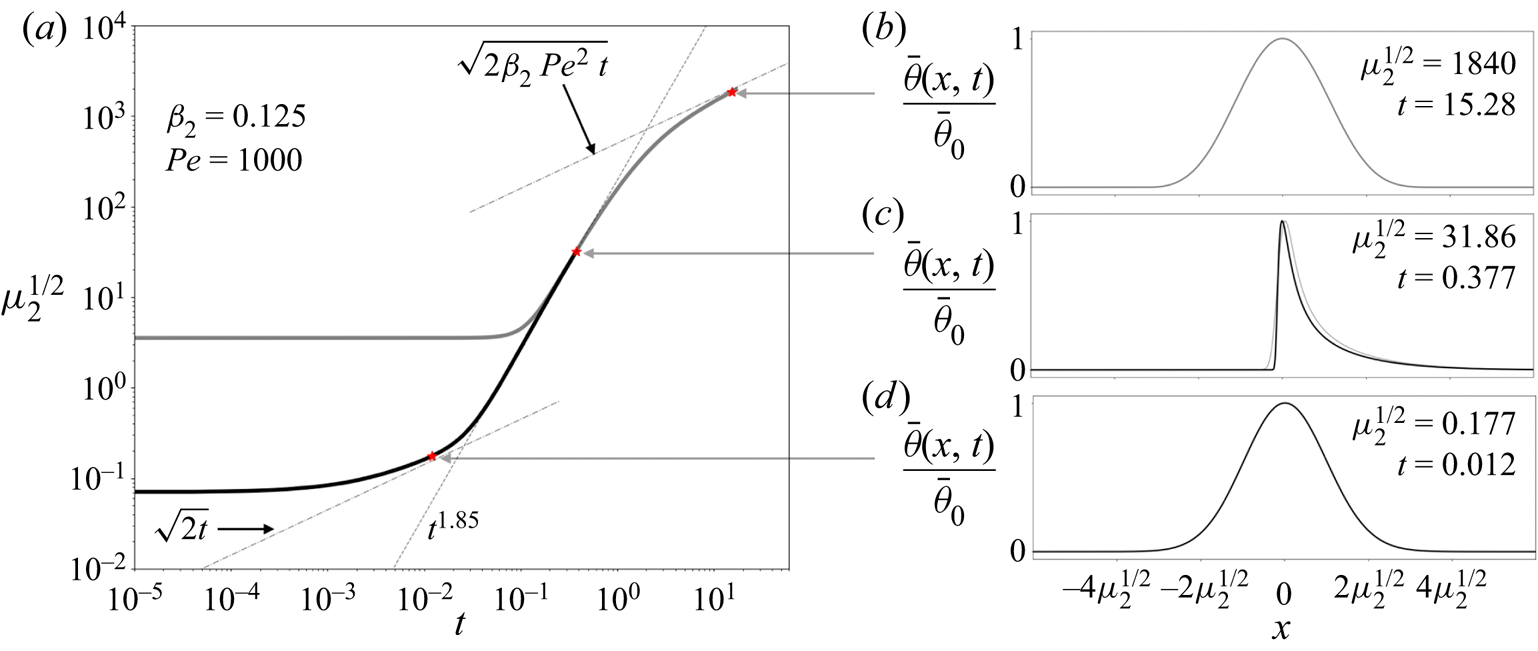
In all steady, laminar parallel shear flows explored, we find that the solution evolves through three distinct stages of dispersion (see figure 9), in agreement with the study by Latini & Bernoff (Reference Latini and Bernoff2001) for the Poiseuille shear flow (that flow corresponds to the polynomial with  $L_d=1$ considered in this study, only shifted by ${\rm \pi}$ in $y$). These stages parallel the three regimes of scalar decay explored in the previous section, and are: an initial pure diffusion stage in which $\mu _{2}=2t$; an intermediate, anomalous (super) diffusion stage; and a final stage of enhanced diffusion $\mu _{2}=2\beta _{2}\,{\textit {Pe}}^2\,t$ that corresponds to Taylor's dispersion (Taylor Reference Taylor1953; Aris Reference Aris1956).
Stages of the dispersion process as a function of time. Each curve represents the evolution of the width of an initially localized tracer patch, with the width defined as the square root of the second moment  $\mu _2$ via (3.11). Each coloured line is associated with a different choice of $y_0$ (see the labels on the right). Also shown are two diffusive curves proportional to $t^{1/2}$, and several super-diffusive power laws (grey lines). The magenta line is for an initial condition that is uniform in the across-stream direction. In all cases, ${\textit {Pe}}=1000$.

Of the three stages of shear dispersion, only the (transient) anomalous diffusion is sensitive to the choice of  $y_0$ in the initial condition (see figure 9), the exception being the ballistic dispersion ( $\sqrt {\mu }\propto t$) associated with a uniform tracer distribution in the cross-shear direction, first studied by Lighthill (see Lighthill Reference Lighthill1966; Latini & Bernoff Reference Latini and Bernoff2001). Table 3 summarizes the power-law approximation to the width $\sqrt {\mu _{2}} = A t^{\gamma _{2}/2}$ in the anomalous diffusion stage for all shear flows considered. In general, our calculated values for $\gamma _2 \approx 4$ for the polynomial shear flow ( $L_d=1$) at $y_0=0$, and $\gamma _2 \approx 3$ for the ( $L_d=1/2$) triangular shear flow (everywhere), coincide with values calculated previously in the literature (Elrick Reference Elrick1962; Rhines & Young Reference Rhines and Young1983; Latini & Bernoff Reference Latini and Bernoff2001; Meunier & Villermaux Reference Meunier and Villermaux2010, Reference Meunier and Villermaux2022).
Parameter pair  $(A, \gamma _2/2)$ that approximates the power-law dependence of width $\sqrt {\mu _2} \approx At^{\gamma _2/2}$ (calculated empirically) in the anomalous diffusion stage. Some of these cases are shown in figure 9.
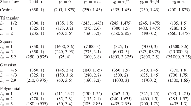
The initial and final stages of the dispersion of an isolated tracer patch are determined by the pure diffusion and Taylor's enhanced diffusion, respectively. The characteristics of these stages are known already from  $\beta _{2}\,{\textit {Pe}}^2$ (§ 3.1) because both processes are self-similar and insensitive to $y_0$, and it is known that transition into Taylor's diffusion happens at $t\gtrsim O(1)$. The time scale for transition from pure diffusion into anomalous diffusion, call it $\tau$, is calculated from the intersection of the two curves $\sqrt {2t}$ and $At^{\gamma _{2}/2}$. Hence $\tau = (2/A^2)^{1/(\gamma _2 - 1)}$, with $\gamma _2$ and $A$ given empirically (table 3).
The envelope of curves  $At^{\gamma _{2}/2}$ associated with the anomalous diffusion stage of shear dispersion in figure 9 shows that $\tau$ is smallest for ballistic dispersion (magenta curves in figure 9). Typically, ballistic dispersion is associated with a uniform initial condition in the cross-shear direction, i.e. a streamwise Gaussian stripe. In this case, the initial tracer patch spans both subdomains $U^*>0$ and $U^*<0$, and its width grows linearly with time as $\sqrt {\mu _{2}} \propto {\textit {Pe}}\,t$. We find that the constant of proportionality ${\sim }0.3 \pm 0.1$ for all shear flows. Using $A=0.3{\textit {Pe}}$, we compute $\tau \approx 20\,{\textit {Pe}}^{-2}$, or $2\times 10^{-5}$ with ${\textit {Pe}}=1000$. Ballistic dispersion also occurs when the initial plume with small cross-shear width is placed at a streamline with infinite shear. (In the square shear flows we see it at $y_0={\rm \pi} /2$ when $L_d=1$, and $y_0=3{\rm \pi} /4$ when $L_d=2$.) In both cases, $\bar {\theta }$ is composed of two asymmetric, long-tailed profiles that separate from one another, as opposed to the single-tailed case in figure 8(c).
The time scale  $\tau$ of transition into anomalous diffusion is delayed the most when the initial condition is placed in regions with zero shear over a wide range of streamlines. The square shear flow is a good example (at $y_0=n{\rm \pi}$, $n$ an integer), in particular at $y_0=0$ and $L_d=5.2$ (red curve in figure 9i). Taking the values $(A, \gamma _2) = (75, 4)$ associated with the square shear flow $L_d=5.2$ from table 3, we find $\tau \approx 0.3$. At this time scale, the plume width transitions from growing diffusively (as $\sqrt {2t}$) to growing with a very steep anomalous diffusion (see red curves in figures 9c,f,i,l).
Contrary to our initial expectations, we found no explicit connection between the time scale  $\tau$ that indicates the transition from pure diffusion to anomalous diffusion in the evolution of the dispersion process, and the inverse scale $k_d^{\pm }$ of transition from (pure modal) anomalous tracer variance decay rate into pure diffusion decay rate. This implies simply that the eigenfunctions $\phi ^e_{2n}, \phi _{2n}^{o}$ also play an important role in determining the transition from Gaussian symmetric to asymmetric cross-flow concentrations, i.e. via a Fourier inversion (see figures 8c,d). Similarly, we found no connection between the values of exponents $s_{\pm}$ from table 2 with the power-law behaviour of $\gamma _2$, not even in the cases where the tracer was initialized at the exact streamlines where shear vanishes. That is, we found no explicit connection between the values $\gamma _2 = 2/3$ and $s_{\pm}=0.75$ derived for the triangular shear flow (e.g. $L_d=1/2$).
The anomalous diffusion stage of shear dispersion is sensitive to the choice of  $y_0$, with implications for the self-similarity of the process. Following Castiglione et al. (Reference Castiglione, Mazzino, Muratore-Ginanneschi and Vulpiani1999) and Ferrari et al. (Reference Ferrari, Manfroi and Young2001), a process is called strongly self-similar whenever the moment's exponent $\gamma _p$ is linear with $p$, i.e. when $\gamma _p = p/\nu$, with $\nu$ an empiric constant. Otherwise, when $\gamma _p$ is piecewise linear, or nonlinear with $p$, the process is called weakly self-similar. An important characteristic of a strongly self-similar process (such as diffusion) is that it satisfies the scaling law
 \begin{equation} \bar{\theta}(x, t)\approx t^{{-}1/\nu}\,\mathcal{C}\left(\frac{x}{t^{1/{\nu}}}\right), \end{equation}
where  $\mathcal {C}$ is a scaling function (e.g. Gaussian in the case of normal diffusion), and $\nu$ is a scaling exponent ( $\nu =2$ for normal diffusion). The scaling law suggests a scaling variable $\xi =x/t^{1/\nu }$, and thus implies that the width of the tracer patch (or equivalently cloud of particles) grows as $t^{1/\nu }$ (Zaburdaev et al. Reference Zaburdaev, Denisov and Klafter2015). Hence a strongly self-similar process is determined entirely by $\nu$. (The values of $\nu$ for flows discussed in the following paragraph are reported in figures 10a–d.)
Moment  $\gamma _p$ dependence on moment index $p$ for three shear flows: (a–d) polynomial flow with $L_d=1$ (Poiseuille-like flow, see figure 2d); (e–h) triangular shear flow with $L_d=1/2$ (see figure 2a); and (i–l) triangular shear flow with $L_d=1$ (also in figure 2a). In (a–d), $y_0$ values, fixed for each column (colour coded to coincide with those in figure 9), are shown. When $\gamma _{p}=p/\nu$, the value of $\nu$ is shown. Grey lines show the pure diffusive behaviour $p/2$.

The quadratic shear flow (polynomial shear with  $L_d=1$) has a strongly self-similar anomalous diffusion stage for various choices of $y_0$, but is weakly self-similar when $y_0={\rm \pi} /4$. The value $\nu \approx 1/2$ at $y_0=0$ coincides with the asymptotic value derived in Latini & Bernoff (Reference Latini and Bernoff2001). A different choice of $y_0$, however, changes the value of $\nu$. The triangular shear flow ( $L_d=1/2$), on the other hand, has a strongly self-similar anomalous diffusion stage that is insensitive to $y_0$. Specifically, $\nu \approx 2/3$ in all cases (figures 10e–h). The triangular shear flow with $L_d=1$ has an anomalous diffusion stage that is strongly self-similar when the plume is initialized in regions with linear shear (figures 10k,l). But when the plume is initialized in regions with no shear, the anomalous diffusion exhibits weak self-similarly (figures 10i,j).
Typically, the scaling exponents  $\nu <2$ are associated with super-diffusive processes such as Levy walks, i.e. stochastics that generalize Brownian diffusion in the sense that the concentration can obey a fractional Fokker–Planck equation (Dubkov et al. Reference Dubkov, Spagnolo and Uchaikin2008). Previous studies have shown that weak self-similar processes fail to be represented by the scaling law (3.14) and obey neither a Fick equation nor other linear equations involving temporal and/or spatial fractional derivatives (Castiglione et al. Reference Castiglione, Mazzino, Muratore-Ginanneschi and Vulpiani1999; Ferrari et al. Reference Ferrari, Manfroi and Young2001). We expand on this by showing that even flows with a strongly self-similar dispersion in their (transient) anomalous diffusion possess a non-unique exponent $\nu$. The exception is the (wide) triangular shear flow ( $L_d=1$), which has a unique scaling exponent, insensitive to the location of the initial condition when the cross-stream width is vanishingly small.
4. Discussion
In this study, we present a new method to compute analytical solutions to the advection–diffusion equation when the advecting velocity is a steady, parallel shear flow, a building block for time-varying flows of the form (1.2). The method relies on the ability to calculate the eigenvalue–eigenvector pairs associated with the non-self-adjoint advection–diffusion operator (2.2), through a convergent truncation of a bi-infinite matrix constructed following a procedure similar to the Floquet–Fourier–Hill method (Deconinck & Kutz Reference Deconinck and Kutz2006). The truncated matrix, for example, implies that for every streamwise Fourier mode  $k$ in a given initial condition with an even Fourier series in the cross-stream direction ( $\chi ^o=0$ in (2.39)), the solution to (2.2) is approximated via
 \begin{equation}
\theta \approx
\mbox{Re}\left\{\sum_{n, l=0}^{R}\chi^*_l A_{2l}^{(2n)}
\phi_{2n}^{e}\exp\left[{\rm
i}k\left(x-\frac{\alpha_0\,{\textit{Pe}}}{2}\,t
\right) - \left(\frac{a_{2n}}{4} + k^2
\right)t \right] \right\} + \theta_{R_{>}},
\end{equation}
\begin{equation}
\theta \approx
\mbox{Re}\left\{\sum_{n, l=0}^{R}\chi^*_l A_{2l}^{(2n)}
\phi_{2n}^{e}\exp\left[{\rm
i}k\left(x-\frac{\alpha_0\,{\textit{Pe}}}{2}\,t
\right) - \left(\frac{a_{2n}}{4} + k^2
\right)t \right] \right\} + \theta_{R_{>}},
\end{equation}
where
 \begin{equation} \theta_{R_{>}} = \sum_{l=R+1}^{\infty}\chi^*_{l}\cos(ly) \cos\left[k\left(x-\frac{\alpha_0\,{\textit{Pe}}}{2}\,t \right) \right] \exp\left[-\left(k^2+l^2 \right)t\right]. \end{equation}
The  $\theta _{R_>}$ contributions coincide with solutions to the diffusion equation, which means that the variance of tracer with cross-flow scales $l_c>R$ decays in the pure diffusion regime.
The analytical method described in § 2.2 is expanded easily to handle shear flows that have a general Fourier series, as well as Neumann (tracer) boundary conditions in the cross-stream direction. Applying Neumann (no-flux) boundary conditions requires three steps, with little modification to the method: (1) increase the periodicity of the shear flow, say from  $P=1$ to $P=2$; (2) restrict the analysis to only half of the domain (so that it gives the appearance of a single-peaked shear flow); (3) given an arbitrary initial condition, consider a second image initial condition, symmetric about the closest boundary $y={\rm \pi}$ or $y = 0$.
Expanding the method to handle a shear flow with arbitrary Fourier series is also straightforward, in a similar way to incorporating Neumann boundary conditions described in the previous paragraph. Again, there are three steps. Given an arbitrary shear flow: (1) construct the flow that is the even-periodic extension of the arbitrary shear flow, which requires extending the original domain by a factor of 2; (2) for an arbitrary initial condition, include an image field initial condition that is equidistant from one of the two (closest) boundaries ( $y=0$ or $y={\rm \pi}$); (3) restrict the analysis to only half of the (new) domain. This approach implies that the tracer satisfies Neumann boundary conditions.
The procedure above implies that a tracer solution with the triangular shear flow ( $L_d=1/2$) and the linear shear flow with Neumann (tracer) boundary conditions arise from the same eigenvalue problem (the EPs in the linear shear case are described in Doering & Horsthemke Reference Doering and Horsthemke1993). The location of the first EP in the linear shear flow described in Doering & Horsthemke (Reference Doering and Horsthemke1993) does not match the location of the first EP of the triangular shear flow, but that can be explained by a rescaling of the domain $M$, which in turn shifts the values of $k$ and ${\textit {Pe}}$. The shifting of the EP locations also happens when the shear-flow periodicity $P$ increases (from $P=1$ to $P=2$ or $3$, as can be seen in the values of $q_{cr}$ in table 1).The equivalence between solutions to (2.2) for the triangular shear flow and the linear shear flow implies that tracer dispersion with the linear shear flow is a strongly self-similar process in all its (shear dispersion) stages, and in the transient anomalous diffusion stage, can likely be model via a fractional Fokker–Planck equation when the initial width is vanishingly small.
It is straightforward to apply the solution method in the presence of time-varying shear flows of the form (1.2), by discretely approximating piecewise constantly any arbitrary, bounded time dependence in  $U_0(t)$. This differs from the approach of Childress & Gilbert (Reference Childress and Gilbert1995), who restrict attention to time-periodic operators, i.e. to time-periodic velocity fields. In addition, the solution method in § 2.2 can be applied also to the case of spatial and temporal variability in diffusivity $\kappa =\kappa (y, t)$, as long as the spatial functional dependence is integrable. In this scenario, the role of ${\rm d}\kappa /{{\rm d}y}$ is identical to the role of the advecting velocity.
The ability to compute analytical solutions for passive scalar tracers governed by (1.1) for spatially varying and time-varying flows, and diffusivities  $\kappa (y, t)$, has important consequences for the study and modelling of biogeochemical tracers. While the inclusion of reaction terms into (1.1) makes the resulting governing equation nonlinear, our solution method can be exploited when the operator splitting approach is used to solve, via alternating ${\rm \Delta} t$ steps of advection–diffusion followed by pure reaction, the resulting advection–diffusion–reaction equation (see Wheeler & Dawson Reference Wheeler and Dawson1987; Rubio, Zalts & El Hasi Reference Rubio, Zalts and El Hasi2008; Kulkarni & Lermusiaux Reference Kulkarni and Lermusiaux2019). Although outside the scope of this study, employing our analytical approach when considering shear flows like those in (1.2) could result in the reduction of spurious mixing associated with numerical advecting schemes (see LeVeque Reference LeVeque2002; Durran Reference Durran2010).
5. Conclusions
The problem of passive scalar dispersion has been studied extensively, but only in a few ideal shear flows and in asymptotic parameter regimes (Taylor Reference Taylor1953; Aris Reference Aris1956; Young et al. Reference Young, Rhines and Garrett1982; Rhines & Young Reference Rhines and Young1983; Doering & Horsthemke Reference Doering and Horsthemke1993; Latini & Bernoff Reference Latini and Bernoff2001; Camassa et al. Reference Camassa, McLaughlin and Viotti2010; Haynes & Vanneste Reference Haynes and Vanneste2014). Here, we present an Eulerian matrix method to compute analytical solutions to the tracer advection–diffusion equation for a broad class of velocity fields and initial conditions. We focus on steady, spatially periodic laminar shear flows, and doubly periodic boundary conditions. But the method allows us to compute solutions to time-varying flows that can be expressed as (1.2), with no-flux (tracer) boundary conditions in the cross-stream direction, and it applies to any shear flow that can be defined via a Fourier series (integrable).
The Eulerian matrix method calculates the eigenvalue spectra of the linear, non-self-adjoint operator of (1.1). We describe thoroughly the properties of the eigenvalue spectrum. In particular, the spectrum properties are shaped by exceptional points with implications for scalar mixing rates, and for the time evolution of localized tracer patches. The analysis also leads to along- and across-stream length scales that determine the effect of the shear.
The Eulerian matrix method is most efficient at low and intermediate Péclet numbers ( ${\textit {Pe}}<10^4$), due to the iterative computation of eigenvalue–eigenfunction pairs. No formal restriction on the value of ${\textit {Pe}}$ applies, however. Also, the present method captures all the stages of shear dispersion. This method therefore complements other approaches that apply to very large ${\textit {Pe}}$ and/or to specific regimes of shear dispersion.
Acknowledgements
The authors would like to thank four anonymous reviewers for their criticisms, comments and suggestions that greatly contributed towards the improvement of our paper. We also thank Dr A. Mani who suggested the potential role that Mathieu's equation with imaginary parameter plays in the solution to the initial-value problem.
Funding
This project was funded by the Johns Hopkins University Institute for Data Intensive Engineering and Science Seed Funding Initiative and NSF grant 1835640.
Declaration of interests
The authors report no conflict of interest.
Author contributions
M.A.J.-U. derived the analytical solution method, computed solutions and performed the necessary simulations for comparison. Both authors contributed equally to analysing results, reaching conclusions and writing the paper.
Appendix A. Analytical expressions of shear flow velocity profiles
Table 4 shows the analytical expressions and Fourier coefficients used in the definition on the main four shear flows in figure 2, and their explicit dependence on the inverse width parameter  $L_d$. All the shear flows share the feature that their maxima are at $y={\rm \pi}$, their minima are at $y=\{0, 2{\rm \pi} \}$, and they converge to a point shear flow as $L_d\rightarrow \infty$, defined as
 \begin{equation} U(y)=\begin{cases} 1, & \text{if } y= {\rm \pi},\\ 0, & \text{otherwise} . \end{cases} \end{equation}
In the case of the polynomial shear flow, we extend it periodically from  $-{\rm \pi} < y < {\rm \pi}$, so that within the interval $y\in [0, 2{\rm \pi} ]$, the velocity is maximum at $y={\rm \pi}$ and decays algebraically to zero at $y=\{0, 2{\rm \pi} \}$. The Fourier coefficients for the polynomial shear flow are
 \begin{equation} \alpha_{m} =\frac{2}{\rm \pi}\int_{0}^{\rm \pi}\frac{y^{2L_d}}{{\rm \pi}^{2L_d}}\cos(my)\,{{\rm d}y}. \end{equation}
The simplest case,  $L_d=1$, yields the quadratic (parabolic) shear flow, which has Fourier coefficients
 \begin{equation} \alpha_{m} = \frac{4({-}1)^{m}}{m^2}. \end{equation}
When  $L_d=2$, the quartic polynomial has Fourier coefficients
 \begin{equation} \alpha_{m} ={-} \frac{8({-}1)^{m}\left( {\rm \pi}^2m^2 - 6 \right) }{m^4} . \end{equation}
Analytical expressions for the flows considered in this study, their dependence on the inverse width parameter  $L_d$, and their Fourier coefficients. For the triangular and square shear flows, the constants are $y_0 = \pi (2L_d-1)/2L_d$ and $y_1 = \pi (2L_d+1)/2L_d$.
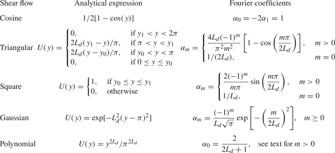
Appendix B. Shift–reflect symmetry and exceptional points
The shift–reflect symmetry of the shear flow is a necessary condition for the presence of exceptional points (EPs). Consider the shifted Hill's equation (compare to (2.10))
 \begin{equation} \frac{{\rm d}^2\phi_{2n}(\tilde{y}-{\rm \pi}/2)}{{\rm d}\tilde{y}^2} + \left[a_{2n} - 2q\,U^*(2\tilde{y}-{\rm \pi})\right]\phi_{2n}(\tilde{y}-{\rm \pi}/2) =0, \end{equation}
and the complex conjugate of Hill's equation for the neighbouring mode,
 \begin{equation} \frac{{\rm d}^2\overline{\phi}_{2n+2}(\tilde{y})}{{{\rm d}y}^2} + \left[\bar{a}_{2n+2} - 2\bar{q}\,U^*(2\tilde{y}) \right]\bar{\phi}_{2n+2}(\tilde{y}) =0, \end{equation}
where the overline indicates the complex conjugate here. As  $q = 2 {\rm i}k\,{Pe}$ is purely imaginary, $-\bar {q}\,U^*(2y) = q\,U^*(2\tilde {y}) = -q\,U^*(2\tilde {y}-{\rm \pi} )$, where the second equality follows for shear flow profiles that possess shift–reflect symmetry. This property makes (B1) and (B2) symmetric with respect to one another in the sense that their real parts are identical while their imaginary parts have opposite signs. Further, a shift-conjugate symmetry of the eigenfunctions is implied, which has the form $\phi _{2n}(\tilde {y}-{\rm \pi} /2) = \bar {\phi }_{2n+2}$ (Ziener et al. Reference Ziener, Rückl, Kampf, Bauer and Schlemmer2012). Even for shear flows that are not shift–reflect symmetric, EPs can occur for sufficiently high modes. The reason is that at sufficiently large modes ( $n$ values), the diagonal element of the $n$th row in (2.21) becomes purely real as the Fourier coefficients that appear in the diagonal decay monotonically.
Appendix C. Reference for variable names
Table 5 contains definitions of some of the most relevant variables of the main text.
Definitions of relevant variables used throughout text.

Appendix D. Numerical validation
A side-by-side comparison between the analytical solution and a numerical simulation is given in figure 11 for the case of a Gaussian initial condition in  $x$ that is uniform in $y$. Two velocity fields are shown: a wide triangular shear flow, and a wide square shear flow. The model solves the advection–diffusion equation with the prescribed (steady) velocity field using a quasi-second-order Adams–Bashforth explicit time stepping scheme and a finite-volume method to calculate the spatial fluxes. The model uses a domain of size $-200{\rm \pi} < x<200{\rm \pi}$, $0< y<2{\rm \pi}$, with $N_{x}=1280$ and ${N_{y}=128}$ grid points. The dimensional parameters are $\kappa =10^{-4}$ m $^2$ s $^{-1}$, $M = 2 {\rm \pi}m$, and the maximum velocity is $U_0 =0.2$ m s $^{-1}$. These choices give ${\textit {Pe}}=2000$ with diffusive time scale $t_{d}=1=M^2/(4 {\rm \pi}^2 \kappa ) = 10^4$ s. The model is the open-source package Oceananigans (Ramadhan et al. Reference Ramadhan, Wagner, Hill, Campin, Churavy, Besard, Souza, Edelman, Ferrari and Marshall2020). As a simple speed comparison, the analytical solution evaluated at the same time-intervals as the stored model output was computed in under 3 minutes with a personal computer (even much less if only a single-time evaluation, say the final one, is needed), whereas the simulation took several hours to perform.
Comparison between (a–d) numerical simulations and (e–h) analytical solutions. The velocity field is (a,b,e,f) the wide triangular shear flow ( $L_d=1/2$, $P=1$), and (c,d,g,h) the wide square shear flow ( $L_d=1$, ${P}=1$). The initial condition is uniform across the flow ( $\varPhi (2\tilde {y})=1$ in (2.37)) for better visualization and localized (Gaussian) at $x = -250$. The white dashed line represents the moving coordinate $x(t)$ that starts at $x(0)=-250$ and moves with the $y$-averaged flow. Both shear flows are shift–reflect symmetric, so the tracer distribution $\theta (t)$ is symmetric (with a ${\rm \pi}$ shift in $y$) with respect to the moving coordinate $x(t)$. Solid white lines at $x=-250$ and near $y=0$ indicate the $x$ location of the initial condition. The matrix truncation parameter is $G=\sqrt {75}$. The numerical simulation results are from the Oceananigans package (Ramadhan et al. Reference Ramadhan, Wagner, Hill, Campin, Churavy, Besard, Souza, Edelman, Ferrari and Marshall2020).

The numerical model solves the tracer equations at centre points, and our eigenvalue approach to solving (2.2) effectively calculates solutions at vorticity points on a C-staggered grid due to our domain (Fourier) mode decomposition (see Durran (Reference Durran2010) for more on grid types). Nonetheless, we interpolate the analytical solution to an equivalent centred grid (or interpolate the numerical solution to corner points), to further quantify the error evolution  ${\rm \Delta} \mathcal {E}$ over time. This is shown in figure 12 for the two flows in figure 11, with the error defined as
 \begin{equation} {\rm \Delta} \mathcal{E}(t) = \sqrt{\frac{k_m}{4{\rm \pi}^2} \int_{0}^{2{\rm \pi}}\int_{-{\rm \pi}/k_m}^{{\rm \pi}/k_m} \left[\theta_{a} - \theta_{b}\right]^2{\rm d} x\,{\rm d} y}, \end{equation}
where  $4{\rm \pi} ^2/k_m$ is the area of the domain as a function of gravest mode $k_m$ (see (2.4a,b)), and $\theta _{a}$ and $\theta _{b}$ represent the analytical and numerical solutions, interpolated onto a common spatial grid. We observe a small and bounded (mean-square) error over the entire tracer evolution (up to when the solution begins re-entry due to periodic boundary conditions). A more complete analysis of the errors (e.g. as a function of grid refinement) remains outside the scope of this paper, but can be done to assess the convergence of discretized operators in two spatial dimensions.

Finally, we note that the error  ${\rm \Delta} \mathcal {E}$ is initially very small but non-zero. This is because in the analytical solution, there are spurious high-frequency non-zero values (errors) typical of ${\ll }1\,\%$ of the solution amplitude, largely uniformly distributed across the domain. These spurious values come from the non-zero cancellation in the triple sum (2.39), and arise from sensitivity to machine precision in the eigenspectra calculation of non-Hermitian linear operators (non-normal matrices). Nonetheless, we found that these spurious high-frequency tracer values associated with very high wavenumber behaviour decay similarly to pure diffusion. For more on the subject of the effect of machine precision on spectra of linear non-Hermitian operators, we refer the reader to Trefethen & Embree (Reference Trefethen and Embree2005).
Appendix E. Gravest eigenvalue asymptotics at small $q$

The dependence of the gravest eigenvalue  $a_{0}$ on $q$ at small $q$ can be approximated easily via regular asymptotic expansion. Following McLachlan (Reference McLachlan1947), consider small- $|q|$ asymptotic approximations to $a_{0}(q)$ and $\phi _{0}(q, \tilde {y})$ of the form
 \begin{gather} a_{0} \approx \beta_{1}q + \beta_{2}q^2 + \cdots, \end{gather}
 \begin{gather}\phi_{0} \approx 1 + q\,C_{1}(2\tilde{y})+q^2\,C_{2}(2\tilde{y}) + \cdots, \end{gather}
where  $C_{1}(2\tilde {y}), C_{2}(2\tilde {y}), \ldots$ are ${\rm \pi}$-periodic functions, and $\beta _{1}, \beta _{2}, \ldots$ are constant coefficients, all to be determined. Because $q=2{\rm i}k\,{\textit {Pe}}$ is purely imaginary, $\beta _{1}$ and $\beta _{2}$ determine the leading-order terms of the imaginary and real components of the eigenvalue in the small- $q$ limit. From (E1), (E2) and the shear flow profile definition (2.6),
 \begin{gather} \phi_{0}^{''} = qC^{''}_{1} + q^2C^{''}_{2} +\cdots, \end{gather}
 \begin{gather}a_{0}\phi_{0} = \left[\beta_{1}q + \beta_{2}q^2 + \cdots \right] \left[1 + q\,C_{1}(2\tilde{y})+q^2\,C_{2}(2\tilde{y}) + \cdots \right], \end{gather}
 \begin{gather}-2qU^*(2\tilde{y})\,\phi_{0}={-}2q\left[\sum_{m=1}^{\infty}\alpha_{m}\cos(2m\tilde{y})\right] \left[1 + q\,C_{1}(2\tilde{y})+q^2\,C_{2}(2\tilde{y}) + \cdots\right]. \end{gather}
Substituting into (2.10) and collecting powers of  $q$ gives the $O(q)$ equation
 \begin{equation} C_{1}^{''} + \beta_{1} = 2\sum_{m=1}^{\infty}\alpha_{m}\cos(2m\tilde{y}). \end{equation}
As we are interested only in periodic solutions,  $\beta _{1}\equiv 0$. Integrating (E6) yields $C_{1} = -\sum _{m=1}^{\infty }(\alpha _{m}/(2m^2))\cos (2m\tilde {y})$. The $O(q^2)$ equation is
 \begin{equation} C_{2}^{''} + \beta_{2} ={-} 2\left(\sum_{m=1}^{\infty}\alpha_{m}\cos(2m\tilde{y})\right) \left(\sum_{m'=1}^{\infty}\frac{\alpha_{m'}}{2m'^2}\cos(2m'\tilde{y})\right). \end{equation}
The right-hand side yields constant terms for  $m=m'$ in the product of the two infinite series (e.g. $2 \cos ^2 (2 \tilde {y}) = \cos (4 \tilde {y}) + 1$). As $C_2$ is periodic, $\beta _{2}$ must exactly balance these constant terms on the right-hand side. Therefore, the coefficient $\beta _{2}$ in (E1) is given exactly by
 \begin{equation} \beta_{2} = \sum_{m=1}^{\infty}\frac{\alpha_{m}^2}{2m^2}, \end{equation}
where  $\alpha _{m}$ are the Fourier coefficients in the definition of the shear flow (2.6). This expression is used in the formula for effective diffusivity (3.5).


 Open access