


1. Introduction
Wall-bounded turbulence has long been one of the most fundamental and extensively studied forms of turbulence, with numerous models proposed to capture its various dynamics and complexities, tailored to specific engineering needs. For example, large-eddy simulations (LES) and wall-modelled LES (WMLES) avoid directly resolving the smaller scales of motions, allowing them to give sufficient faithfulness in replicating turbulence in a wide array of engineering applications, such as flows over aircraft (Gao et al. Reference Gao, Zhang, Cheng and Samtaney2019; Lozano-Durán et al. Reference Lozano-Durán, Bose and Moin2022), urban environments (Giometto et al. Reference Giometto, Christen, Meneveau, Fang, Krafczyk and Parlange2016), atmospheric boundary layers (Porté-Agel et al. Reference Porté-Agel, Meneveau and Parlange2000) or in supercritical environments (Mahesh et al. Reference Mahesh, Constantinescu, Apte, Iaccarino, Ham and Moin2006; Matheis & Hickel Reference Matheis and Hickel2018), without the inhibitive computational costs of direct numerical simulations (DNS). Methods such as the hybrid Reynolds-averaged Navier–Stokes/LES methods and WMLES have been identified as possessing the greatest potential for external aerodynamics at high Reynolds numbers for the near future (Slotnick et al. Reference Slotnick, Khodadoust, Alonso, Darmofal, Gropp, Lurie and Mavriplis2014). While these methods are inherently useful, the drastic truncation of small scales and, in the case of WMLES, the inner-layer dynamics, also leaves room for improvement in modelling the missing components (Larsson et al. Reference Larsson, Kawai, Bodart and Bermejo-Moreno2016; Bae et al. Reference Bae, Lozano-Durán, Bose and Moin2018; Fu et al. Reference Fu, Karp, Bose, Moin and Urzay2021, Reference Fu, Bose and Moin2022). In particular, since the small scales are modelled instead of directly resolved, their relationship to the larger scales in turbulence has garnered particular attention for researchers since it could further push the boundaries of LES-based methods and other turbulence modelling techniques at affordable costs (Li et al. Reference Li, Baars, Marusic and Hutchins2023). Furthermore, in experiments, due to physical limitations, measurement points and their spatial configurations are usually restricted to those far from the wall, with large areas of flow not captured due to the need for spacing out the measurement locations, further necessitating quantifiable relationships of interscale dynamics. With advances in the generation of extensive high-fidelity data and experimental techniques, there has been an increasing number of effective attempts at predicting near-wall turbulence or reconstructing turbulent features based on limited flow information.
With predicting or reconstructing turbulence in mind, we can roughly categorise them through two major approaches. The first treats turbulence as a random process, where even if the fundamental equations of motions, the governing Navier–Stokes equations (NSE), are explicitly invoked, they are seen as filters (Landau & Lifshitz Reference Landau and Lifshitz1959) that alter the random noise input and its effects. This approach poses questions regarding the statistics of turbulent flow, where they are mostly reliant on data-driven techniques. One such model, inspired by the attached eddy hypothesis (AEH) proposed by Townsend (Reference Townsend1951, Reference Townsend1961, Reference Townsend1976), is the attached eddy model (AEM). It considers wall-bounded turbulence as a field of randomly distributed eddies rooted to the wall, where Townsend (Reference Townsend1976) predicted the statistics of turbulence without any prescribed structures of the flow, but only the self-similarity of attached eddies and a constant characteristic velocity scale (Marusic & Monty Reference Marusic and Monty2019). Perry & Chong (Reference Perry and Chong1982) further formalised the AEM based on the structures of hairpin vortices, and while the existence of such vortices is still somewhat debated in fully developed turbulent flow (Eitel-Amor et al. Reference Eitel-Amor, Örlü, Schlatter and Flores2015), there has been extensive evidence supporting the AEM (see Wu & Moin Reference Wu and Moin2009; Jodai & Elsinga Reference Jodai and Elsinga2016; Marusic & Monty Reference Marusic and Monty2019).
The second and prevailing methodology of interest in this paper is based on treating turbulence as a deterministic high-dimensional dynamical system of interacting coherent structures (Jiménez Reference Jiménez2018). Any randomness is readily ignored and avoided, effectively treating the prescribed system as deterministic over indubitably limited time or spatial domains. In particular, this approach aims to extract and capture coherent structures, which are simple enough for predictions in theoretical models, and turbulent statistics may be used as inputs into the model. A popular method is based on the linearised NSE, composing a linear relationship between a nonlinear input forcing term and the output responses of velocity, pressure and temperature fluctuations (McKeon & Sharma Reference McKeon and Sharma2010; Hwang & Cossu Reference Hwang and Cossu2010). The resolvent operator captures this linear relationship through Fourier transformations in the temporal and spatial directions (McKeon & Sharma Reference McKeon and Sharma2010). Building upon this input–output formalism, many credible prediction models have been devised using only limited data to predict the full flow statistics (see Towne, Lozano-Durán & Yang Reference Towne, Lozano-Durán and Yang2020; Martini et al. Reference Martini, Cavalieri, Jordan, Towne and Lesshafft2020; Ying et al. Reference Ying, Liang, Li and Fu2023) or instantaneous velocity fluctuations (see Amaral et al. Reference Amaral, Cavalieri, Martini, Jordan and Towne2021; Arun, Bae & McKeon Reference Arun, Bae and McKeon2023). Furthermore, other data-driven methods such as modal decomposition has also received considerable attention, which include but are not limited to the proper orthogonal decomposition (Lumley Reference Lumley1967), its spectral counterpart the spectral proper orthogonal decomposition (Lumley Reference Lumley1970) and the dynamic mode decomposition (Schmid Reference Schmid2010). The decomposed modes inherently manifest spatial and temporal coherence, linking coherence structures with many data-driven techniques, without the need for the NSE or prescribed structures. Towne, Schmidt & Colonius (Reference Towne, Schmidt and Colonius2018) further established connections between the aforementioned modal decomposition-based methods and the NSE-based resolvent analysis, which offers further understanding of the NSE.
Furthermore, the structures of the hairpin vortices, which inspired the AEM by Perry & Chong (Reference Perry and Chong1982), can also be regarded as coherent structures and have also enabled further understanding of the AEH and wall-bounded turbulence, allowing for the physical insights into the flow. These coherent structures and other physical mechanisms within turbulence, have and will continue to play a large role in the development of theoretical turbulent models, such as the discovery of streaks in the buffer region (Kline et al. Reference Kline, Reynolds, Schraub and Runstadler1967) or the large-scale motions (LSMs), very large-scale motions (VLSMs) and self-similar motions found in the logarithmic and outer regions of turbulent boundary layers (Lozano-Durán et al. Reference Lozano-Durán, Bae and Encinar2020).
The mechanisms that inspired the turbulence model in question are the large-scale superposition and amplitude modulation of the small-scale structures in turbulent boundary layers. Near-wall structures, often described as autonomous or self-sustaining, propagate and sustain without the need for external influences (see Jiménez & Pinelli Reference Jiménez and Pinelli1999; Panton Reference Panton2001; Schoppa & Hussain Reference Schoppa and Hussain2002). However, due to the limitations of data when these studies were conducted, turbulence structures in the logarithmic region and their influences on the near-wall structures were not well understood. With the development of experimental and computational capabilities, many studies have found external influences from the large-scale, log-region events on the near-wall small-scale motions.
Abe, Kawamura & Choi (Reference Abe, Kawamura and Choi2004) and Hutchins & Marusic (Reference Hutchins and Marusic2007a ) found that these logarithmic region structures, termed LSMs, VLSMs or superstructures, influence the streamwise velocity fluctuations deep into the near-wall regions, where they superimpose a footprint (or mean shift) on the near-wall velocity fluctuations. These superstructure events are a spanwise alternative sequence of highly elongated negative and positive streamwise velocity fluctuations centred in the logarithmic region (Hutchins & Marusic Reference Hutchins and Marusic2007a ), where it exerts low-wavenumber, outer-scaled energy into the near-wall region. Similar footprinting phenomenon have also been found in Rayleigh–Bénard turbulence (Berghout, Baars & Krug Reference Berghout, Baars and Krug2021), where numerous other studies have found many different interscale interactions, where LSMs exert influence on near-wall flows, e.g. near-wall streaks (Zhou, Xu & Jiménez Reference Zhou, Xu and Jiménez2022), compressible near-wall structures (Zhou et al. Reference Zhou, Wang, Zhang, Huang and Xu2024), frictional drag (Hwang & Sung Reference Hwang and Sung2017), etc.
Mathis, Hutchins & Marusic (Reference Mathis, Hutchins and Marusic2009) further found that they also modulate the amplitude of near-wall signals with varying degrees of strength in the wall-normal direction within experimental studies. Chung & McKeon (Reference Chung and McKeon2010) also validated this large-scale amplitude modulation mechanism in LES of long channel flows. Utilising the Hilbert transformation, a scale-decomposition of the streamwise velocity signal was performed, separating the velocity fluctuations into a large-scale and a small-scale signal, where Mathis et al. (Reference Mathis, Hutchins and Marusic2009) showed that the large-scale signal modulates the small-scale signal in the viscous and buffer layers. The amplitude modulation mechanism has been further extended to frequency modulation (Ganapathisubramani et al. Reference Ganapathisubramani, Hutchins, Monty, Chung and Marusic2012) and observed via phase analysis (Jacobi & McKeon Reference Jacobi and McKeon2013). It has also been discovered in other types of flows, such as air jets (Fiscaletti, Ganapathisubramani & Elsinga Reference Fiscaletti, Ganapathisubramani and Elsinga2015), permeable-wall turbulence (Kim et al. Reference Kim, Blois, Best and Christensen2020), other velocity components and instantaneous Reynolds shear stress (Talluru et al. Reference Talluru, Baidya, Hutchins and Marusic2014), atmospheric boundary layers (Salesky & Anderson Reference Salesky and Anderson2018; Liu, He & Zheng Reference Liu, He and Zheng2023), turbulence at transcritical condition (Li, Zhang & Ihme Reference Li, Zhang and Ihme2024), etc. Jacobi et al. (Reference Jacobi, Chung, Duvvuri and McKeon2021) also formalised the interactions between scales in wall-bounded turbulence, where a transfer function derived from the NSEs was found to be similar to that of the amplitude modulation mechanism. Amplitude modulation in compressible flows has also been investigated (see Helm & Martin Reference Helm and Martin2013, Reference Helm and Martin2014; Yu & Xu Reference Yu and Xu2022; Yu et al. Reference Yu, Fu, Tang, Yuan and Xu2023; Yu et al. Reference Yu, Zhao, Du, Yuan and Xu2025), but the number of studies has been relatively fewer and less extensive than its incompressible counterpart.
The combination of the superposition and amplitude modulation inspired the latter work of a predictive model for wall-bounded turbulence by Marusic, Mathis & Hutchins (Reference Marusic, Mathis and Hutchins2010) and Baars, Hutchins & Marusic (Reference Baars, Hutchins and Marusic2016), specifically, the inner–outer interaction model (IOIM). As with any model, the relationships of the model components across flow parameters are of particular importance. In the following, we detail the IOIM framework and pose questions, specifically about the model parameter variations.
2. The IOIM
The IOIM (Baars et al. Reference Baars, Hutchins and Marusic2016), and its previous iteration, the eponymously named MMH (Marusic–Mathis–Hutchins) model (Marusic et al. Reference Marusic, Mathis and Hutchins2010), based on the large-scale coherence and the aforementioned amplitude modulation and superposition in high-Reynolds-number wall-bounded turbulence flow, has been used to predict streamwise velocity fluctuations within the inner region using a known input from the logarithmic region.
The IOIM framework requires only a large-scale velocity signature from an outer position in the logarithmic region, usually its geometric centre point, which is empirically determined as
 $y_O^+ = 3.9 \textit{Re}_\tau ^{({1}/{2})}$
(Marusic et al. Reference Marusic, Mathis and Hutchins2010, Reference Marusic, Monty, Hultmark and Smits2013). Here,
$y_O^+ = 3.9 \textit{Re}_\tau ^{({1}/{2})}$
(Marusic et al. Reference Marusic, Mathis and Hutchins2010, Reference Marusic, Monty, Hultmark and Smits2013). Here,
 $y$
denotes the wall-normal position,
$y$
denotes the wall-normal position,
 $u$
is the raw streamwise velocity fluctuation, decomposed from the raw velocity signal and its mean profile,
$u$
is the raw streamwise velocity fluctuation, decomposed from the raw velocity signal and its mean profile,
 $U$
. The friction velocity is
$U$
. The friction velocity is
 $u_\tau$
, the fluid kinematic viscosity is
$u_\tau$
, the fluid kinematic viscosity is
 $\nu$
, and the superscript
$\nu$
, and the superscript
 $^+$
denotes the inner-scaling such that
$^+$
denotes the inner-scaling such that
 $y^+ \equiv y u_\tau / \nu$
and
$y^+ \equiv y u_\tau / \nu$
and
 $u^+ \equiv u / u_\tau$
;
$u^+ \equiv u / u_\tau$
;
 $\textit{Re}_\tau = u_\tau h / \nu$
is the friction Reynolds number where
$\textit{Re}_\tau = u_\tau h / \nu$
is the friction Reynolds number where
 $h$
is the half-channel height or boundary layer thickness. The predicted signal can be computed through the following equation:
$h$
is the half-channel height or boundary layer thickness. The predicted signal can be computed through the following equation:
 \begin{align} \underbrace {u_P^+(y^+, t^+)}_{\mathrm{Prediction}} = \underbrace {u^*(y^+, t^+)\{1 + \varGamma (y^+) u_S^+(y^+, t^+ - \tau _a^+)\}}_{\text{Amplitude modulate}} + \hspace {0.15em} \underbrace {u_S^+(y^+, t^+)}_{\mathrm{Superposition}}, \quad 0 \lt y^+ \lt y^+_O, \end{align}
where
 $u_P^+$
corresponds to the desired or prediction signal,
$u_P^+$
corresponds to the desired or prediction signal,
 $u^*$
is the universal signal, where the input
$u^*$
is the universal signal, where the input
 $u_S^+$
, extracted from the raw outer signal
$u_S^+$
, extracted from the raw outer signal
 $u_O^+$
. The amplitude modulation coeffecient,
$u_O^+$
. The amplitude modulation coeffecient,
 $\varGamma$
, is a parameter of the IOIM, which requires calibration, representing the strength of the amplitude modulation mechanism. The universal signal,
$\varGamma$
, is a parameter of the IOIM, which requires calibration, representing the strength of the amplitude modulation mechanism. The universal signal,
 $u^*$
, is meant to represent the small-scale signals, rid of any superposition or amplitude modulation effects. All velocity fluctuations time series are synchronised by the inner-scaled time
$u^*$
, is meant to represent the small-scale signals, rid of any superposition or amplitude modulation effects. All velocity fluctuations time series are synchronised by the inner-scaled time
 $t^+ = tu_\tau ^2 / \nu$
. We note that the input
$t^+ = tu_\tau ^2 / \nu$
. We note that the input
 $u_S^+$
within the amplitude modulate component contains a time shift,
$u_S^+$
within the amplitude modulate component contains a time shift,
 $\tau _a^+$
, meant to account for the relative shift between the near-wall, small-scale signal and its modulator, the superposition component. This shift is wall-normal height dependent and Reynolds number invariant, i.e.
$\tau _a^+$
, meant to account for the relative shift between the near-wall, small-scale signal and its modulator, the superposition component. This shift is wall-normal height dependent and Reynolds number invariant, i.e.
 $\tau ^+_a = \tau ^+_a(y^+)$
(Baars et al. Reference Baars, Talluru, Hutchins and Marusic2015).
$\tau ^+_a = \tau ^+_a(y^+)$
(Baars et al. Reference Baars, Talluru, Hutchins and Marusic2015).
Using the linear transfer kernel,
 $\widetilde {H}_L$
, we obtain the superposition component
$\widetilde {H}_L$
, we obtain the superposition component
 $u_S^+(y^+, t^+)$
from the known input outer layer signal,
$u_S^+(y^+, t^+)$
from the known input outer layer signal,
 $u_O^+(y_O^+)$
, as follows:
$u_O^+(y_O^+)$
, as follows:
 \begin{equation} u_S^+(y^+) = \mathcal{F}^{-1}\{\hat {u}_S(y^+;f^+)\} = \mathcal{F}^{-1}\left \{\widetilde {H}_L(y^+;f^+)\mathcal{F}\left [u_O^+(y_O^+)\right ]\right \}, \end{equation}
where
 $\hat {u}(f^+) = \mathcal{F}[u^+(t^+)]$
denotes the Fourier transformation of
$\hat {u}(f^+) = \mathcal{F}[u^+(t^+)]$
denotes the Fourier transformation of
 $u^+$
and
$u^+$
and
 $f^+ \equiv U^+_m / \lambda _x^+$
is the frequency determined by the local mean velocity,
$f^+ \equiv U^+_m / \lambda _x^+$
is the frequency determined by the local mean velocity,
 $U^+_m \equiv U^+(y_O^+)$
. We compute
$U^+_m \equiv U^+(y_O^+)$
. We compute
 $\widetilde {H}_L$
through a spectral linear stochastic estimation (SLSE) framework as follows:
$\widetilde {H}_L$
through a spectral linear stochastic estimation (SLSE) framework as follows:
 \begin{equation} \widetilde {H}_L(f^+) = |H_L|_{\textit{filt}} e^{j \phi (f^+)} = \left (\frac {|\langle \hat {u}(f^+) \breve {\hat {u}}_O(f^+) \rangle |}{\langle |\hat {u}_O(f^+) |^2\rangle }\right )_{\textit{filt}}\hspace {-0.5em}e^{j \phi (f^+)}, \end{equation}
where the subscript
 $_{{filt}}$
denotes a
$_{{filt}}$
denotes a
 $\pm 25\,\%$
bandwidth moving filter (BMF),
$\pm 25\,\%$
bandwidth moving filter (BMF),
 $| \boldsymbol{\cdot }|$
denotes the modulus,
$| \boldsymbol{\cdot }|$
denotes the modulus,
 $\langle \boldsymbol{\cdot }\rangle$
denotes ensemble averaging,
$\langle \boldsymbol{\cdot }\rangle$
denotes ensemble averaging,
 $\breve {(\boldsymbol{\cdot })}$
denotes the complex conjugates,
$\breve {(\boldsymbol{\cdot })}$
denotes the complex conjugates,
 $j$
is the imaginary unit
$j$
is the imaginary unit
 $\sqrt {-1}$
and
$\sqrt {-1}$
and
 $\phi (f^+)$
is the phase of the kernel.
$\phi (f^+)$
is the phase of the kernel.
This model embeds its scale separation into the scale-dependent gains,
 $|\widetilde {H}_L(f^+)|$
, without the need for a prior user choice of scale separation. The IOIM framework is capable of accurately reconstructing the velocity signal based on (2.1) and has been validated across a range of high-friction Reynolds numbers from 2800 to
$|\widetilde {H}_L(f^+)|$
, without the need for a prior user choice of scale separation. The IOIM framework is capable of accurately reconstructing the velocity signal based on (2.1) and has been validated across a range of high-friction Reynolds numbers from 2800 to
 $1.4 \times 10^6$
for experimental turbulent boundary layers. For more details regarding model parameter calibrations, we refer the readers to the original papers (see Mathis, Hutchins & Marusic Reference Mathis, Hutchins and Marusic2011; Baars et al. Reference Baars, Hutchins and Marusic2016).
$1.4 \times 10^6$
for experimental turbulent boundary layers. For more details regarding model parameter calibrations, we refer the readers to the original papers (see Mathis, Hutchins & Marusic Reference Mathis, Hutchins and Marusic2011; Baars et al. Reference Baars, Hutchins and Marusic2016).
2.1. Applications and further developments of the IOIM
The IOIM model has been used extensively in various applications. Notably, the IOIM framework or its amplitude modulation mechanism has been validated in other types of turbulent flows other than canonical wall-bounded flows, such as free stream turbulence (see Dogan et al. Reference Dogan, Hanson and Ganapathisubramani2016, Reference Dogan, Hearst and Ganapathisubramani2017), turbulent flows with different wall conditions (see Pathikonda & Christensen Reference Pathikonda and Christensen2017; Efstathiou & Luhar Reference Efstathiou and Luhar2018; Blackman, Perret & Mathis Reference Blackman, Perret and Mathis2019), unsteady turbulence (Lu et al. Reference Lu, He, Wang and Liu2024) and different driving pressures (see Harun et al. Reference Harun, Monty, Mathis and Marusic2013; Mathis et al. Reference Mathis, Marusic, Hutchins, Monty and Harun2015; Dróżdż et al. Reference Dróżdż, Niegodajew, Romańczyk and Elsner2023). Through this framework, enhanced amplitude modulation has also been found in non-canonical flows, such as boundary layers over rough walls (Monty et al. Reference Monty, Chong, Mathis, Hutchins, Marusic and Allen2009; Squire et al. Reference Squire, Baars, Hutchins and Marusic2016; Wu, Christensen & Pantano Reference Wu, Christensen and Pantano2019) or permeable surfaces (Kim et al. Reference Kim, Blois, Best and Christensen2020; Khorasani, Luhar & Bagheri Reference Khorasani, Luhar and Bagheri2024), or those including modified outer structures, for example, upstream dynamic roughness (Duvvuri & McKeon Reference Duvvuri and McKeon2015) and synthetic large-scale signals from plasma actuators (Lozier, Thomas & Gordeyev Reference Lozier, Thomas and Gordeyev2022). Li et al. (Reference Li, Baars, Marusic and Hutchins2023) further quantified the effects of the amplitude modulation coefficient in these non-canonical flows under the IOIM framework.
The IOIM framework has also been deployed together with other mathematical techniques and models. Yin et al. (Reference Yin, Huang and Xu2017, Reference Yin, Huang and Xu2018) showed that turbulent fluctuations in minimal flow units are congruent with the universal signal extracted from the IOIM framework. Mäteling & Schröder (Reference Mäteling and Schröder2022) also analysed the inner–outer interactions via a multivariate empirical mode decomposition in channel flows. The IOIM framework has been further extended to supersonic and hypersonic turbulent boundary layers, where in addition to the prediction of streamwise velocity fluctuations, models for temperature and density fluctuations using the strong Reynolds analogy have also been developed (Helm & Martin Reference Helm and Martin2013, Reference Helm and Martin2014), similarly based on the mechanism of superposition, amplitude modulation and phase shift within the IOIM framework. Yu & Xu (Reference Yu and Xu2022) furthered the investigation of the IOIM in the compressible regime, incorporating density variations and developed an alternative method for computing the amplitude modulation coefficients and the universal signal. Yu et al. (Reference Yu, Fu, Tang, Yuan and Xu2023) also used minimal flow units to demonstrate the capabilities of the IOIM in compressible flows by utilising its universal signals in the study of Mach number effects and for the reconstruction of streamwise, wall-normal and spanwise velocity components in addition to temperature fluctuations. Moreover, the IOIM showed great agreement with AEM. Based on a completely different mechanism, the IOIM framework was utilised in the study of attached eddies’ inclination angles in compressible flows (Bai, Cheng & Fu Reference Bai, Cheng and Fu2024) and streamwise wall-shear stress fluctuations (Cheng & Fu Reference Cheng and Fu2022), where Cheng & Fu (Reference Cheng and Fu2022) has shown quantitative consistency between the two models for incompressible flow.
2.2. A physical perspective on the IOIM
While the amplitude modulation mechanism of near-wall signals by LSMs and VLSMs is the motivation behind the IOIM framework (Marusic et al. Reference Marusic, Mathis and Hutchins2010), it is perhaps more physically insightful to view the framework from another perspective. Given the long-standing success of the AEM not only in prediction but also in allowing a better understanding of the physical turbulent structures, attached and detached eddies in this instance, it is pertinent, if possible, to relate these two models and the turbulence mechanisms at large.
Figure 1 provides an illustration of the physical structures in wall-bounded turbulence in accordance with the AEH, with the reference location
 $y_O^+$
from the IOIM also labelled. We can see that the velocity signal at the reference location,
$y_O^+$
from the IOIM also labelled. We can see that the velocity signal at the reference location,
 $u_O^+$
, is influenced by several factors: the self-similar attached eddies, LSMs / VLSMs, and the local detached eddies in the logarithmic layer. Through the linear transfer kernel, the larger-scale eddies – LSMs, VLSMs and attached eddies are extracted, effectively discarding the smaller-scale detached eddies, resulting in the coherent signal (or superposition signal),
$u_O^+$
, is influenced by several factors: the self-similar attached eddies, LSMs / VLSMs, and the local detached eddies in the logarithmic layer. Through the linear transfer kernel, the larger-scale eddies – LSMs, VLSMs and attached eddies are extracted, effectively discarding the smaller-scale detached eddies, resulting in the coherent signal (or superposition signal),
 $u_S^+(y^+)$
. The magnitude of this coherent signal extracted from
$u_S^+(y^+)$
. The magnitude of this coherent signal extracted from
 $u_O^+$
, or the large-scale effect from
$u_O^+$
, or the large-scale effect from
 $u_O^+$
, decreases as we near the wall since the differences between
$u_O^+$
, decreases as we near the wall since the differences between
 $u_O^+$
and
$u_O^+$
and
 $u_P^+$
are greater. The signal at
$u_P^+$
are greater. The signal at
 $u_P^+$
contains information regarding the coherent structures that
$u_P^+$
contains information regarding the coherent structures that
 $u_O^+$
lacks, such as the smaller, self-similar attached eddies as hypothesised by AEH and the increasingly viscous-dominated detached eddies, leading to a decrease in coherence between the known signal and the desired signal.
$u_O^+$
lacks, such as the smaller, self-similar attached eddies as hypothesised by AEH and the increasingly viscous-dominated detached eddies, leading to a decrease in coherence between the known signal and the desired signal.
An illustration of the turbulent structures within wall-bounded turbulence based on the AEH; not to physical scale. The red dashed line indicates the reference layer within the IOIM framework, where the known velocity signal
 $u_O^+(y_O^+)$
lies. The LSMs/VLSMs are shown to be detached from the wall for illustration purposes, but they may extend well into the logarithmic layer, the near-wall region and may even be attached to the wall, exerting their influence across the flow. The known velocity signal is then used to predict
$u_O^+(y_O^+)$
lies. The LSMs/VLSMs are shown to be detached from the wall for illustration purposes, but they may extend well into the logarithmic layer, the near-wall region and may even be attached to the wall, exerting their influence across the flow. The known velocity signal is then used to predict
 $u_P^+(y_P^+)$
for
$u_P^+(y_P^+)$
for
 $0 \lt y_P^+ \lt y_O^+$
based on
$0 \lt y_P^+ \lt y_O^+$
based on
 $\varGamma$
and
$\varGamma$
and
 $u^*$
.
$u^*$
.

This decrease in the large-scale coherent signal must be accounted for in order to accurately predict
 $u_P^+$
, leading to the amplitude modulation component,
$u_P^+$
, leading to the amplitude modulation component,
 $\varGamma u_S^+$
in (2.1), where
$\varGamma u_S^+$
in (2.1), where
 $\varGamma$
increases to compensate for the decrease in
$\varGamma$
increases to compensate for the decrease in
 $u_S^+$
. As we move towards the wall, where our desired prediction signal lies, we come into contact with more and more smaller-scale self-similar attached eddies, increasing the proportion of energy that was contributed from them. At the same time, the effects of the LSMs and VLSMs weaken within the logarithmic region. The increase in self-similar, smaller, wall-attached eddies and lessened effects from LSMs and VLSMs correspond well to the previously observed amplitude modulation coefficient profiles where
$u_S^+$
. As we move towards the wall, where our desired prediction signal lies, we come into contact with more and more smaller-scale self-similar attached eddies, increasing the proportion of energy that was contributed from them. At the same time, the effects of the LSMs and VLSMs weaken within the logarithmic region. The increase in self-similar, smaller, wall-attached eddies and lessened effects from LSMs and VLSMs correspond well to the previously observed amplitude modulation coefficient profiles where
 $\varGamma$
reaches a plateau region with a stationary point as
$\varGamma$
reaches a plateau region with a stationary point as
 $y^+$
decreases (Baars et al. Reference Baars, Hutchins and Marusic2016) around the logarithmic region due to their combined effects. The amplitude modulation coefficient can therefore be described as the net effect of LSMs, VLSMs and attached eddies all together, where it acts as a compensator for the variation in the strength of physical structures that cannot be captured from
$y^+$
decreases (Baars et al. Reference Baars, Hutchins and Marusic2016) around the logarithmic region due to their combined effects. The amplitude modulation coefficient can therefore be described as the net effect of LSMs, VLSMs and attached eddies all together, where it acts as a compensator for the variation in the strength of physical structures that cannot be captured from
 $u_O^+$
and the decrease in the large-scale coherence in
$u_O^+$
and the decrease in the large-scale coherence in
 $u_S^+$
; as we move downwards through the logarithmic region, the increase in the population density of attached eddies increases
$u_S^+$
; as we move downwards through the logarithmic region, the increase in the population density of attached eddies increases
 $\varGamma$
, and the decrease in LSMs/VLSMs effects decreases
$\varGamma$
, and the decrease in LSMs/VLSMs effects decreases
 $\varGamma$
. As we continue to move from the logarithmic region to the viscous sublayer near the wall, the viscous-dominated detached eddies within the viscous sublayer and any even smaller scale effects that cannot be suitably quantified can be seen as the universal signal,
$\varGamma$
. As we continue to move from the logarithmic region to the viscous sublayer near the wall, the viscous-dominated detached eddies within the viscous sublayer and any even smaller scale effects that cannot be suitably quantified can be seen as the universal signal,
 $u^*$
, where all their effects are captured within. The amplitude modulation coefficient within the viscous sublayer then becomes dominated by the near-wall viscous eddies and increases as observed in the previously obtained profiles, compensating for any larger-scale signals that cannot be extracted from
$u^*$
, where all their effects are captured within. The amplitude modulation coefficient within the viscous sublayer then becomes dominated by the near-wall viscous eddies and increases as observed in the previously obtained profiles, compensating for any larger-scale signals that cannot be extracted from
 $u_O^+$
.
$u_O^+$
.
From this viewpoint, the resulting IOIM framework thereby allows us to quantify the effects of the different structures of turbulence, naturally providing a decomposition of not just the coherence and incoherence but rather displaying the effects of existing structures. Near-wall viscous effects are captured by
 $u^*$
, where its effects counteract the amplitude modulation effects brought on by the culmination of eddies within
$u^*$
, where its effects counteract the amplitude modulation effects brought on by the culmination of eddies within
 $u_O^+$
near the reference layer, such that its effect is captured by
$u_O^+$
near the reference layer, such that its effect is captured by
 $\varGamma$
. As we move towards the wall, (2.1) represents this balance between the decrease in the large-scale coherent structures,
$\varGamma$
. As we move towards the wall, (2.1) represents this balance between the decrease in the large-scale coherent structures,
 $u_S^+$
, the universal near-wall detached eddies,
$u_S^+$
, the universal near-wall detached eddies,
 $u^*$
, and the increase in the compensator,
$u^*$
, and the increase in the compensator,
 $\varGamma u_S^+$
, for the missing physical structures in the known signal
$\varGamma u_S^+$
, for the missing physical structures in the known signal
 $u^+_O(y^+_O)$
such as the smaller self-similar attached eddies below
$u^+_O(y^+_O)$
such as the smaller self-similar attached eddies below
 $y^+_O$
.
$y^+_O$
.
We note that the discussions regarding LSMs and VLSMs here and hereafter are somewhat simplified. While the IOIM framework perceives the energy cascade only from the large scales to the small scales, recent studies have found that there is a significant amount of reverse interscale energy transfer, where the small-scale motions transfer energy to the large scales in the streamwise and spanwise velocity components (Cho, Hwang & Choi Reference Cho, Hwang and Choi2018). The impact of this, if any, on the inner–outer interaction is yet to be understood, since this suggests a self-sustaining energy cascade loop. In any case, the viewpoint from the IOIM framework is that from the large scale to the small scale, but we felt that it was pertinent to highlight the reverse mechanism and its significance on turbulence transport also.
With IOIM seemingly applicable in a variety of flows, the natural questions that follow are the robustness of its parameters in these different types of flows. Are the IOIM’s parameters ‘universal’, particularly across incompressible and compressible flow? Can we quantitatively capture the parameter variation, if any, so we can provide a universal IOIM by altering key parameters? What do the quantitative differences in the IOIM’s parameters tell us about the physical turbulence structures at large, in particular, the structures previously defined from the AEH? While many papers have independently answered some of the questions partially, the following attempts to holistically answer these questions within the realm of canonical incompressible and compressible wall-bounded turbulence.
2.3. Outline
The rest of the paper is organised as follows. In § 3, the DNS data used is described, followed by illustrations and analyses of the IOIM’s parameters, including the linear transfer kernel
 $\widetilde {H}_L$
, the universal signal
$\widetilde {H}_L$
, the universal signal
 $u^*$
and the amplitude modulation coefficient
$u^*$
and the amplitude modulation coefficient
 $\varGamma$
in § 4. In this section, we will attempt to capture empirical trends within the IOIM framework to quantify particular variations, particularly between incompressible and compressible flows. We will link these quantitative differences to the physical perspective from AEH we provided in § 2.2. A recapitulative discussion on the universality of the IOIM model and its parameters closes out the paper in § 5.
$\varGamma$
in § 4. In this section, we will attempt to capture empirical trends within the IOIM framework to quantify particular variations, particularly between incompressible and compressible flows. We will link these quantitative differences to the physical perspective from AEH we provided in § 2.2. A recapitulative discussion on the universality of the IOIM model and its parameters closes out the paper in § 5.
3. Data
3.1. Incompressible flow
A set of time-resolved, incompressible channel turbulence DNS data at
 $\textit{Re}_\tau = 186, 547, 934$
and
$\textit{Re}_\tau = 186, 547, 934$
and
 $2003$
were generated by a comprehensively validated methodology (Kim, Moin & Moser Reference Kim, Moin and Moser1987; Del Á lamo & Jiménez Reference Del Á lamo and Jiménez2003; Hoyas & Jiménez Reference Hoyas and Jiménez2006, Reference Hoyas and Jiménez2008; Lozano-Durán & Jiménez Reference Lozano-Durán and Jiménez2014), where its computational parameters are shown in table 1.
$2003$
were generated by a comprehensively validated methodology (Kim, Moin & Moser Reference Kim, Moin and Moser1987; Del Á lamo & Jiménez Reference Del Á lamo and Jiménez2003; Hoyas & Jiménez Reference Hoyas and Jiménez2006, Reference Hoyas and Jiménez2008; Lozano-Durán & Jiménez Reference Lozano-Durán and Jiménez2014), where its computational parameters are shown in table 1.
Parameters of the incompressible channel DNS. Here,
 $L_x, L_y$
and
$L_x, L_y$
and
 $L_z$
denote the computational domain in the streamwise, wall-normal and spanwise directions, respectively. The inner-scaled times steps of the DNS,
$L_z$
denote the computational domain in the streamwise, wall-normal and spanwise directions, respectively. The inner-scaled times steps of the DNS,
 $\delta _t^+ = \delta _t u_\tau ^2 / \nu$
, and
$\delta _t^+ = \delta _t u_\tau ^2 / \nu$
, and
 $(u_\tau T)/h$
is the eddy turnover time to ensure statistical convergence. The outer reference location used to calibrate the IOIM model for their corresponding cases is denoted by
$(u_\tau T)/h$
is the eddy turnover time to ensure statistical convergence. The outer reference location used to calibrate the IOIM model for their corresponding cases is denoted by
 $y_O^+$
and
$y_O^+$
and
 $\eta$
denotes the Kolmogorov length scale, such that the quantity
$\eta$
denotes the Kolmogorov length scale, such that the quantity
 $max _y (h/\eta)$
denotes the largest ratio between the largest scale and the smallest scale.
$max _y (h/\eta)$
denotes the largest ratio between the largest scale and the smallest scale.

3.2. Compressible flow
A series of DNS of supersonic channel flows were conducted at a range of bulk Mach numbers
 ${\textit {Ma}}_b = U_b / c_w = 0.8, 1.5$
and
${\textit {Ma}}_b = U_b / c_w = 0.8, 1.5$
and
 $3$
as listed in table 2, where
$3$
as listed in table 2, where
 $U_b$
is the bulk velocity and
$U_b$
is the bulk velocity and
 $c_w$
is the speed of sound at the wall temperature, and bulk Reynolds number
$c_w$
is the speed of sound at the wall temperature, and bulk Reynolds number
 $\textit{Re}_b = \rho _b U_b h / \mu _w$
, where
$\textit{Re}_b = \rho _b U_b h / \mu _w$
, where
 $\rho _b$
is the bulk density and
$\rho _b$
is the bulk density and
 $\mu _w$
is the wall dynamic viscosity. All the cases were computed with the computational domain of
$\mu _w$
is the wall dynamic viscosity. All the cases were computed with the computational domain of
 $(L_x, L_y, L_z) = (4\pi h, 2h, 2\pi h)$
. Previous studies have validated the data such that the energy-containing motions in the logarithmic and outer regions can be resolved by this computational domain (Agostini & Leschziner Reference Agostini and Leschziner2014; Cheng & Fu Reference Cheng and Fu2024). The simulations were conducted using a finite-difference code, which solves the three-dimensional compressible NSE along with a passive scalar transport equation. More details on the computational methodology can be found in Cheng & Fu (Reference Cheng and Fu2024).
$(L_x, L_y, L_z) = (4\pi h, 2h, 2\pi h)$
. Previous studies have validated the data such that the energy-containing motions in the logarithmic and outer regions can be resolved by this computational domain (Agostini & Leschziner Reference Agostini and Leschziner2014; Cheng & Fu Reference Cheng and Fu2024). The simulations were conducted using a finite-difference code, which solves the three-dimensional compressible NSE along with a passive scalar transport equation. More details on the computational methodology can be found in Cheng & Fu (Reference Cheng and Fu2024).
Parameters of the compressible channel DNS. The superscript
 $^*$
denotes semilocally scaled wall-normal positions,
$^*$
denotes semilocally scaled wall-normal positions,
 $y^*$
, and friction Reynolds number,
$y^*$
, and friction Reynolds number,
 $\textit{Re}_\tau ^*$
. The computational grid points in the streamwise, wall-normal and spanwise directions are denoted as
$\textit{Re}_\tau ^*$
. The computational grid points in the streamwise, wall-normal and spanwise directions are denoted as
 $N_x, N_y$
and
$N_x, N_y$
and
 $N_z$
. Here
$N_z$
. Here
 $\Delta _x^+$
and
$\Delta _x^+$
and
 $\Delta _z^+$
are the streamwise and spanwise grid resolutions in viscous units, where
$\Delta _z^+$
are the streamwise and spanwise grid resolutions in viscous units, where
 $\Delta y^+_{\textit{min}}$
and
$\Delta y^+_{\textit{min}}$
and
 $\Delta y^+_{\textit{max}}$
denote the finest and coarsest resolution in the wall-normal direction, also in viscous units.
$\Delta y^+_{\textit{max}}$
denote the finest and coarsest resolution in the wall-normal direction, also in viscous units.

4. Results
The IOIM for the compressible flow cases is computed using density-weighted velocity fluctuations,
 $\sqrt {\rho }u''$
, where
$\sqrt {\rho }u''$
, where
 $u''$
denotes the fluctuations from Favre averaging, and semilocally scaled wall-normal coordinates and friction Reynolds number (Trettel & Larsson Reference Trettel and Larsson2016; Griffin, Fu & Moin Reference Griffin, Fu and Moin2021), denoted as
$u''$
denotes the fluctuations from Favre averaging, and semilocally scaled wall-normal coordinates and friction Reynolds number (Trettel & Larsson Reference Trettel and Larsson2016; Griffin, Fu & Moin Reference Griffin, Fu and Moin2021), denoted as
 $y^*$
and
$y^*$
and
 $Re^*_\tau$
, respectively, for suitable comparisons between compressible flow and incompressible flow. The use of the density-weighted velocity fluctuations follows the practice of many previous studies (including but not limited to Patel et al. (Reference Patel, Peeters, Boersma and Pecnik2015), Sciacovelli, Cinnela & Gloerfelt (Reference Sciacovelli, Cinnela and Gloerfelt2017), Hirai, Pecknik & Kawai (Reference Hirai, Pecknik and Kawai2021), Huang, Duan & Choudhanri (Reference Huang, Duan and Choudhanri2022), Yu & Xu (Reference Yu and Xu2022), Cheng & Fu (Reference Cheng and Fu2023) and Bai et al. (Reference Bai, Cheng and Fu2024)), where a motivating factor is that the statistical characteristics of
$Re^*_\tau$
, respectively, for suitable comparisons between compressible flow and incompressible flow. The use of the density-weighted velocity fluctuations follows the practice of many previous studies (including but not limited to Patel et al. (Reference Patel, Peeters, Boersma and Pecnik2015), Sciacovelli, Cinnela & Gloerfelt (Reference Sciacovelli, Cinnela and Gloerfelt2017), Hirai, Pecknik & Kawai (Reference Hirai, Pecknik and Kawai2021), Huang, Duan & Choudhanri (Reference Huang, Duan and Choudhanri2022), Yu & Xu (Reference Yu and Xu2022), Cheng & Fu (Reference Cheng and Fu2023) and Bai et al. (Reference Bai, Cheng and Fu2024)), where a motivating factor is that the statistical characteristics of
 $\overline {\rho u'' u''} / \tau _w$
in compressible boundary layers resemble those of
$\overline {\rho u'' u''} / \tau _w$
in compressible boundary layers resemble those of
 $\overline {u'^2}^+$
in incompressible wall turbulence (Huang et al. Reference Huang, Duan and Choudhanri2022; Cheng & Fu Reference Cheng and Fu2023), where the overline
$\overline {u'^2}^+$
in incompressible wall turbulence (Huang et al. Reference Huang, Duan and Choudhanri2022; Cheng & Fu Reference Cheng and Fu2023), where the overline
 $\overline {(\boldsymbol{\cdot })}$
denotes Reynolds averaging. We also note that the use of the fluctuations from Favre-average or Reynolds-average results in no discernible differences. Using this opportunity, we can also assess the suitability of this scaling for the consideration of compressibility overall.
$\overline {(\boldsymbol{\cdot })}$
denotes Reynolds averaging. We also note that the use of the fluctuations from Favre-average or Reynolds-average results in no discernible differences. Using this opportunity, we can also assess the suitability of this scaling for the consideration of compressibility overall.
4.1. Linear transfer kernel –
 $\widetilde {H}_L$

The transfer kernel is the key to separating the scales within the streamwise velocity fluctuations and is the first step in constructing the IOIM. Figure 2 shows the linear transfer kernel profile for the incompressible flow cases in table 1 with an increase in Reynolds numbers from figures 2(a) to 2(d).
Comparisons of the final linear transfer kernel
 $\widetilde {H}_L$
for the incompressible flow cases, with the panels labelled for the cases in table 1: (a) Re186, (b) Re547, (c) Re934 and (d) Re2003, respectively.
$\widetilde {H}_L$
for the incompressible flow cases, with the panels labelled for the cases in table 1: (a) Re186, (b) Re547, (c) Re934 and (d) Re2003, respectively.

The linear transfer kernel can be interpreted as the coherent correlation between the signal along the wall-normal direction and the signal at the outer reference height at each wavelength, where it extracts the coherent large-scale signal from the outer reference layer, which is superposed at each near-wall position. While at much higher Reynolds number flow (
 $\textit{Re}_\tau \approx 7450, 13\,300$
), Baars et al. (Reference Baars, Hutchins and Marusic2016) suggested that the linear transfer kernel is visually indistinguishable within the wall-normal range that it considered, which was used for brief predictions of flow from
$\textit{Re}_\tau \approx 7450, 13\,300$
), Baars et al. (Reference Baars, Hutchins and Marusic2016) suggested that the linear transfer kernel is visually indistinguishable within the wall-normal range that it considered, which was used for brief predictions of flow from
 $2800 \leqslant \textit{Re}_\tau \leqslant 19\,000$
, upon closer inspection, we observe that there are significant differences in the linear transfer kernel within the range
$2800 \leqslant \textit{Re}_\tau \leqslant 19\,000$
, upon closer inspection, we observe that there are significant differences in the linear transfer kernel within the range
 $186 \leqslant \textit{Re}_\tau \leqslant 2003$
.
$186 \leqslant \textit{Re}_\tau \leqslant 2003$
.
Figures 2 and 3(a) shows several differences in the linear transfer kernel at increasing Reynolds numbers for incompressible flow, where the transfer kernel more visibly shows an initial flat region at the largest wavelengths before a secondary flat region when it reaches the absolute peak value of unity at higher Reynolds numbers. This flat region is not present at the lowest Reynolds number case Re186, where a flat region only exists after reaching the peak absolute value
 $|\widetilde {H}_L| = 1$
. We also observe that the linear transfer kernel gain is smaller as the Reynolds number increases at each
$|\widetilde {H}_L| = 1$
. We also observe that the linear transfer kernel gain is smaller as the Reynolds number increases at each
 $y^+$
. Furthermore, figure 3(b) shows a clear quadratic trend in the smallest wall-normal heights where the transfer kernel gain reaches the maximum value. However, this quadratic trend in
$y^+$
. Furthermore, figure 3(b) shows a clear quadratic trend in the smallest wall-normal heights where the transfer kernel gain reaches the maximum value. However, this quadratic trend in
 ${\textrm {argmin}}_{y^+}|\widetilde {H}_L({y^+, \lambda _x^+}_{\textit{max}})| = 1$
may be due to the selection of the reference outer-layer location,
${\textrm {argmin}}_{y^+}|\widetilde {H}_L({y^+, \lambda _x^+}_{\textit{max}})| = 1$
may be due to the selection of the reference outer-layer location,
 $y^+ = 3.9 \textit{Re}_\tau ^{({1}/{2})}$
.
$y^+ = 3.9 \textit{Re}_\tau ^{({1}/{2})}$
.
The incompressible flow cases’ linear transfer kernels (a) magnitudes at the largest inner-scaled wavelengths
 ${\lambda _x^+}_{\textit{max}}$
, and (b) for comparing
${\lambda _x^+}_{\textit{max}}$
, and (b) for comparing
 ${\textrm {argmin}}_{y^+} |\widetilde {H}_L({y^+, \lambda _x^+}_{\textit{max}})| = 1$
, i.e. the smallest
${\textrm {argmin}}_{y^+} |\widetilde {H}_L({y^+, \lambda _x^+}_{\textit{max}})| = 1$
, i.e. the smallest
 $y^+$
where
$y^+$
where
 $|\widetilde {H}_L(y^+, {\lambda _x^+}_{\textit{max}})| = 1$
, for their respective
$|\widetilde {H}_L(y^+, {\lambda _x^+}_{\textit{max}})| = 1$
, for their respective
 $y^+_O$
. The dashed–dotted line indicates a quadratic best-fit line, where
$y^+_O$
. The dashed–dotted line indicates a quadratic best-fit line, where
 $R^2$
indicate its coefficient of determination.
$R^2$
indicate its coefficient of determination.

Absolute values of the linear transfer kernel profiles displayed as a surface for the incompressible flow cases.

Figure 4 further displays this trend, where at
 $y^+ \gt 1$
, the absolute value of the linear transfer kernel is larger across any shared wavelengths at decreasing Reynolds numbers, such that at each of the same wavelengths, there is a larger proportion of the outer signal energy superimposed onto the near-wall signals at lower Reynolds numbers. Therefore, since the lower Reynolds number cases dominate at any common wavelengths and for
$y^+ \gt 1$
, the absolute value of the linear transfer kernel is larger across any shared wavelengths at decreasing Reynolds numbers, such that at each of the same wavelengths, there is a larger proportion of the outer signal energy superimposed onto the near-wall signals at lower Reynolds numbers. Therefore, since the lower Reynolds number cases dominate at any common wavelengths and for
 $y^+ \gt 1$
, we have that
$y^+ \gt 1$
, we have that
 \begin{equation} |\widetilde {H}_L(y^+, \lambda _x^+)|_{\mathrm{Re186}} \gt |\widetilde {H}_L(y^+, \lambda _x^+)|_{\mathrm{Re547}} \gt |\widetilde {H}_L(y^+, \lambda _x^+)|_{\mathrm{Re934}} \gt |\widetilde {H}_L(y^+, \lambda _x^+)|_{\mathrm{Re2003}}, \end{equation}
for
 $y^+ \gt 1$
. In addition, when combined with figure 3, we can see that the trend at the largest wavelengths extends through the entire range of wavelengths and wall-normal heights, indicating the variation and non-universality of the linear transfer kernel within the investigated Reynolds number range via its differing degrees of large-scale influence as seen in the large differences in the linear transfer kernel profiles evidenced in figures 3 and 4.
$y^+ \gt 1$
. In addition, when combined with figure 3, we can see that the trend at the largest wavelengths extends through the entire range of wavelengths and wall-normal heights, indicating the variation and non-universality of the linear transfer kernel within the investigated Reynolds number range via its differing degrees of large-scale influence as seen in the large differences in the linear transfer kernel profiles evidenced in figures 3 and 4.
Comparisons of the final linear transfer kernel
 $\widetilde {H}_L$
for the compressible flow cases, with the panels labelled for the cases in table 2: (a) Ma08Re171, (b) Ma08Re384, (c) Ma08Re783, (d) Ma15Re144, (e) Ma15Re394, (f) Ma15Re773, (g) Ma30Re140, and (h) Ma30Re396.
$\widetilde {H}_L$
for the compressible flow cases, with the panels labelled for the cases in table 2: (a) Ma08Re171, (b) Ma08Re384, (c) Ma08Re783, (d) Ma15Re144, (e) Ma15Re394, (f) Ma15Re773, (g) Ma30Re140, and (h) Ma30Re396.

While incompressible flow can show common trends of the linear transfer kernel across differing Reynolds numbers, the effect of varying compressibility on the linear transfer kernel across similar Reynolds numbers is explored next within compressible flow cases. Figure 5 shows the linear transfer kernel profile for the compressible flow cases in table 2. We compare the figures across different Mach numbers with a similar
 $\textit{Re}_\tau ^*$
, i.e. figures 5(a,d,g), 5(b,e,h) and 5(c,f). Again, the profiles have trends similar to those of the incompressible cases across Reynolds numbers. In figure 6(a), we can observe the profiles of the linear transfer kernel at the largest wavelengths, where cases with fairly similar friction Reynolds numbers exhibit a more similar profile in shape. Again, two flat regions are only observable at the largest wavelengths at higher Reynolds numbers, whereas the cases Ma08Re171, Ma15Re144 and Ma30Re140, only display one flat region at the largest wavelengths. A more noticeable quadratic trend with respect to the Reynolds number can be observed in figure 6(b) for the smallest wall-normal heights, which attain a linear transfer kernel magnitude of unity at the maximum wavelength. However, this ‘similarity’ across Reynolds numbers may be attributed to the outer reference layer location, determined by
$\textit{Re}_\tau ^*$
, i.e. figures 5(a,d,g), 5(b,e,h) and 5(c,f). Again, the profiles have trends similar to those of the incompressible cases across Reynolds numbers. In figure 6(a), we can observe the profiles of the linear transfer kernel at the largest wavelengths, where cases with fairly similar friction Reynolds numbers exhibit a more similar profile in shape. Again, two flat regions are only observable at the largest wavelengths at higher Reynolds numbers, whereas the cases Ma08Re171, Ma15Re144 and Ma30Re140, only display one flat region at the largest wavelengths. A more noticeable quadratic trend with respect to the Reynolds number can be observed in figure 6(b) for the smallest wall-normal heights, which attain a linear transfer kernel magnitude of unity at the maximum wavelength. However, this ‘similarity’ across Reynolds numbers may be attributed to the outer reference layer location, determined by
 $y^*_O = 3.9 {\textit{Re}_\tau ^*}^{({1}/{2})}$
, where, again, an obvious quadratic trend may exist. The effect of this location on the IOIM is further explored in § 4.4. We can also notice some Mach number effects from figure 6(a).
$y^*_O = 3.9 {\textit{Re}_\tau ^*}^{({1}/{2})}$
, where, again, an obvious quadratic trend may exist. The effect of this location on the IOIM is further explored in § 4.4. We can also notice some Mach number effects from figure 6(a).
We can observe that for the cases with the same Reynolds number, the greater Mach number leads to the magnitude of the linear transfer kernel being smaller at the maximum wavelength at the same wall-normal height. Given that the magnitude of the transfer kernel is decreasing as
 $\lambda _x^+$
decreases, it indicates that the imprint of a large-scale signal that can be separated from the actual velocity signal decreases as the Mach number increases, such that an increase in compressibility leads to a decrease in the footprint left by the large-scale signals at a particular wall-normal height for similar friction Reynolds numbers.
$\lambda _x^+$
decreases, it indicates that the imprint of a large-scale signal that can be separated from the actual velocity signal decreases as the Mach number increases, such that an increase in compressibility leads to a decrease in the footprint left by the large-scale signals at a particular wall-normal height for similar friction Reynolds numbers.
Similar to figure 3 but for the compressible flow cases. Wall-normal coordinates are semilocally scaled for an equivalent non-dimensionalisation to incompressible flow cases.

Comparisons of the linear transfer kernels between the incompressible and compressible flow cases at the largest wavelengths. Similar to figures 3(a) and 6(a), but a similar Reynolds number range separates the cases: (a)
 $140 \leqslant Re^*_\tau \leqslant 186$
, (b)
$140 \leqslant Re^*_\tau \leqslant 186$
, (b)
 $384 \leqslant Re^*_\tau \leqslant 547$
and (c)
$384 \leqslant Re^*_\tau \leqslant 547$
and (c)
 $773 \leqslant Re^*_\tau \leqslant 934$
. Panel (d) is similar to figures 3(b) and 6(b), where it plots
$773 \leqslant Re^*_\tau \leqslant 934$
. Panel (d) is similar to figures 3(b) and 6(b), where it plots
 ${\textrm {argmin}}_{y^+} |\widetilde {H}_L({y^*, \lambda _x^+}_{\textit{max}})| = 1$
, i.e. the smallest
${\textrm {argmin}}_{y^+} |\widetilde {H}_L({y^*, \lambda _x^+}_{\textit{max}})| = 1$
, i.e. the smallest
 $y^*$
where
$y^*$
where
 $|\widetilde {H}_L(y^*, {\lambda _x^+}_{\textit{max}})| = 1$
, for their respective
$|\widetilde {H}_L(y^*, {\lambda _x^+}_{\textit{max}})| = 1$
, for their respective
 $y^*_O$
. The dash–dotted line indicates a quadratic best-fit line, where its coefficient of determination is the
$y^*_O$
. The dash–dotted line indicates a quadratic best-fit line, where its coefficient of determination is the
 $R^2$
indicated in (d).
$R^2$
indicated in (d).

Similar to figure 4, but for both the incompressible and compressible flow cases corresponding to tables 1 and 2, respectively. The surfaces generated are split into a range of Reynolds numbers similar to figure 7, where the
 $\textit{Re}_\tau ^*$
ranges between
$\textit{Re}_\tau ^*$
ranges between
 $140 \leqslant Re^*_\tau \leqslant 186$
for (a) and (b),
$140 \leqslant Re^*_\tau \leqslant 186$
for (a) and (b),
 $384 \leqslant Re^*_\tau \leqslant 547$
for (c) and (d),
$384 \leqslant Re^*_\tau \leqslant 547$
for (c) and (d),
 $773 \leqslant Re^*_\tau \leqslant 934$
for (e) and (f). The panels are plotted such that each row contains a similar friction Reynolds number range. Panels (a), (c) and (e) are comparisons between the incompressible cases and the compressible cases where
$773 \leqslant Re^*_\tau \leqslant 934$
for (e) and (f). The panels are plotted such that each row contains a similar friction Reynolds number range. Panels (a), (c) and (e) are comparisons between the incompressible cases and the compressible cases where
 ${\textit {Ma}}_b = 0.8$
. Panels (b), (d) and (f), are comparisons between the compressible linear transfer kernel profiles.
${\textit {Ma}}_b = 0.8$
. Panels (b), (d) and (f), are comparisons between the compressible linear transfer kernel profiles.

To more directly compare the effect of compressibility on the linear transfer kernel, figure 7 compares the linear transfer kernels between the incompressible and compressible flow cases at the largest wavelengths at a similar friction Reynolds number range. It is clear that at a similar Reynolds number range, the increasing compressibility leads to a decrease in the absolute value of the linear transfer kernel at the largest wavelengths. Furthermore, in figure 7(d), while we can still observe a quadratic trend between the wall-normal heights where the absolute value of the linear transfer kernel first reaches unity, it is evident that the quadratic trend found is not as strong since the coefficient of determination is smaller compared with figures 3(b) and 6(b), where the incompressible and compressible flow cases were fitted independently. This weaker correlation, albeit only slightly, occurs when both incompressible flow cases and compressible flow cases are fitted together, indicating subtle differences in the essential dynamics and the interscale energy transfer derived from the linear transfer kernel. This further suggests that an increase in compressibility leads to the superstructures in the outer layer having less of a superimposing effect on the near-wall signals at similar Reynolds numbers, where the energy transfer between the superstructures and the near-wall region within compressible wall-bounded flows is less than their incompressible counterparts.
Figure 8 further highlights the differences in magnitudes between the linear transfer kernels among all the cases, where it shows the surface generated from the linear transfer kernel among its shared wavelengths. We observe that the absolute values of the linear transfer kernels are larger at lower compressibility, particularly near the wall. However, this is not as clear at the transition from incompressibility to compressibility, where the relatively lower Reynolds number and the lower compressibility within the subsonic range lead to differing energy transfer dominance across the wall-normal range, as seen in figure 8(a,c,e). Within this lower compressibility range, the footprint left by the superimposing outer signal is much weaker as compressibility increases, but only close to the wall, suggesting that an introduction of compressibility and its effects impede the energy transfer from the outer region to the inner region. A further increase in compressibility to within the supersonic range, as seen in figure 8(b,d,f), shows an increase in the resistance of energy transfer between the layers, wherein the outer regions, the absolute value of the linear transfer kernel is dominated by the lower
 ${\textit {Ma}}_b$
cases.
${\textit {Ma}}_b$
cases.
While this damping phenomenon, caused by the introduction of compressibility, is clear, the degree of damping or reduction of energy transfer between wall-normal layers is yet to be thoroughly investigated. The IOIM framework cannot directly quantify the limits on energy transfer in a holistic way, but the linear transfer kernel may yet provide some insights into the energy transfer depth between the outer-layer superstructures and the near-wall layers. The absolute value of the linear transfer kernel decreases as we move away from the outer reference layer until it reaches a distinct initial flat region around
 $10 \lt y^* \lt 50$
, as observed in the linear transfer kernel profiles at relatively higher Reynolds numbers, where they have a similar degree of energy transfer at this initial flat region range. Beyond this range, the near-wall effects might inhibit further energy transfer at a further depth beyond
$10 \lt y^* \lt 50$
, as observed in the linear transfer kernel profiles at relatively higher Reynolds numbers, where they have a similar degree of energy transfer at this initial flat region range. Beyond this range, the near-wall effects might inhibit further energy transfer at a further depth beyond
 $y^* \approx 10$
as the linear transfer kernel magnitudes decrease significantly. The near-wall effects observed inhibiting further energy transfer, in combination with the superposed signals of the superstructures in the logarithmic regions, may be one of the major contributors to this build-up of energy as observed in distributions in the wall-normal distributions of the streamwise turbulent stresses, as it peaks at
$y^* \approx 10$
as the linear transfer kernel magnitudes decrease significantly. The near-wall effects observed inhibiting further energy transfer, in combination with the superposed signals of the superstructures in the logarithmic regions, may be one of the major contributors to this build-up of energy as observed in distributions in the wall-normal distributions of the streamwise turbulent stresses, as it peaks at
 $y^* = 15$
. Linking back to figure 1, the extracted large scales indicate a lessened effect from LSMs, VLSMs and attached eddies as compressibility increases.
$y^* = 15$
. Linking back to figure 1, the extracted large scales indicate a lessened effect from LSMs, VLSMs and attached eddies as compressibility increases.
This finding, where compressibility inhibits the energy transfer between the layers, agrees well with other studies independent of the IOIM framework (for example, see Smits et al. (Reference Smits, Spina, Alving, Smith, Fernando and Donovan1989)), and further reinforces the veracity of the SLSE-based linear transfer kernel, where it suitably displays the damping effects of compressibility and its increased aversion to energy transfer towards the wall, especially within the supersonic range. However, from a modelling perspective, these strong variations observed in the linear transfer kernel profiles, particularly as compressibility varies, are a downside of this IOIM framework since we cannot directly interchange the linear transfer kernels freely between different flow parameters and cases.
4.2. Universal signal –
$u^*$

The universal signal is the small-scale or incoherent signal contained within a velocity signal without any large-scale effects. Figure 9 shows the universal signals’ premultiplied energy spectra for the incompressible flow cases, where the universal signal does display strong universality across Reynolds numbers. However, the Re186 case, with the lack of a sufficiently strong large-scale signal, struggles to extract a refined universal signal within the IOIM framework, especially close to the wall. Revisiting the linear transfer kernel profiles, the Re186 case is one with a distinctly different shape than its higher Reynolds number peers, which may suggest that the linear transfer kernel shape, in particular, its lack of an initial flat region is an indicator of the presence of the large-scale signal and the amplitude modulation phenomenon if the standard reference location of
 $y_O^+ \equiv 3.9 \textit{Re}_\tau ^{({1}/{2})}$
is used.
$y_O^+ \equiv 3.9 \textit{Re}_\tau ^{({1}/{2})}$
is used.
Comparisons of the ‘detrended’ universal signal
 $u^*$
between the incompressible flow cases, where the panels are labelled identically to the cases in figure 2. Isocontour representations of the premultiplied energy spectra of the universal signal,
$u^*$
between the incompressible flow cases, where the panels are labelled identically to the cases in figure 2. Isocontour representations of the premultiplied energy spectra of the universal signal,
 $k_x \phi _{u^* u^*}$
, are indicated by the solid lines with colours as per table 1. The dashed lines represent the isocontours of the premultiplied energy spectra of the streamwise velocity fluctuations,
$k_x \phi _{u^* u^*}$
, are indicated by the solid lines with colours as per table 1. The dashed lines represent the isocontours of the premultiplied energy spectra of the streamwise velocity fluctuations,
 $k_x \phi _{uu}$
, whereas the vertical dash–dotted line indicates the reference layer location,
$k_x \phi _{uu}$
, whereas the vertical dash–dotted line indicates the reference layer location,
 $y_O^+$
.
$y_O^+$
.

Figure 10 further shows the similarities across
 $\textit{Re}_\tau$
, where the proportion of total streamwise fluctuation energy across
$\textit{Re}_\tau$
, where the proportion of total streamwise fluctuation energy across
 $y^+$
is shown. While figure 10(a) displays obvious variations due to the differing reference layers, through normalisation with
$y^+$
is shown. While figure 10(a) displays obvious variations due to the differing reference layers, through normalisation with
 $y_O^+$
in figure 10(b), we can observe that the proportions of the total streamwise energy contained within the universal signals are similar. As the Reynolds number increases (
$y_O^+$
in figure 10(b), we can observe that the proportions of the total streamwise energy contained within the universal signals are similar. As the Reynolds number increases (
 $\textit{Re}_\tau \leqslant 2003$
) and we approach the Re2003 case, where large-scale effects are distinctly significant, the proportion of universal signal can be modelled with
$\textit{Re}_\tau \leqslant 2003$
) and we approach the Re2003 case, where large-scale effects are distinctly significant, the proportion of universal signal can be modelled with
 \begin{equation} \frac {\sum _{k_x} k_x \phi _{u^* u^*}}{\sum _{k_x} k_x \phi _{u u}} \approx A \left \{1 - \exp {\left [B\left (\frac {y^+}{y^+_O} - 1\right ) \right ]}\right \}, \end{equation}
where
 $A = 0.99$
and
$A = 0.99$
and
 $B = 7.5$
. This shows remarkable similarities across Reynolds numbers despite the different points of scale separation embedded within the linear transfer kernel, where the fraction of small scales contained within each flow is similar. It is the increasingly larger scales that drive the major differences between the flows, such as the greater amount of low-wavenumber energy at the inner spectral peak and the emergence of the outer spectral peak (Hutchins & Marusic Reference Hutchins and Marusic2007b
). Further observations of the limiting behaviour of the universal signal at high Reynolds number and whether it still adheres to (4.2) are needed to further ascertain this finding since this study only goes up to
$B = 7.5$
. This shows remarkable similarities across Reynolds numbers despite the different points of scale separation embedded within the linear transfer kernel, where the fraction of small scales contained within each flow is similar. It is the increasingly larger scales that drive the major differences between the flows, such as the greater amount of low-wavenumber energy at the inner spectral peak and the emergence of the outer spectral peak (Hutchins & Marusic Reference Hutchins and Marusic2007b
). Further observations of the limiting behaviour of the universal signal at high Reynolds number and whether it still adheres to (4.2) are needed to further ascertain this finding since this study only goes up to
 $\textit{Re}_\tau = 2003$
. However, we believe that (4.2) serves as a basis for the universal signal proportion, and suitable changes to the equation parameters
$\textit{Re}_\tau = 2003$
. However, we believe that (4.2) serves as a basis for the universal signal proportion, and suitable changes to the equation parameters
 $A$
and
$A$
and
 $B$
can be made to adjust for the differences, if there are any, at higher Reynolds numbers.
$B$
can be made to adjust for the differences, if there are any, at higher Reynolds numbers.
One-dimensional premultiplied energy spectra for the incompressible flow cases scaled by their total energies as a function of the wall-normal heights,
 $y^+$
, in (a). Panel (b) shows the same, but in scaled wall-normal coordinates by the reference location,
$y^+$
, in (a). Panel (b) shows the same, but in scaled wall-normal coordinates by the reference location,
 $y^+ / y_O^+$
. The dashed line models the variation in the proportion of energy contained within the universal signals across this scaled wall-normal height, where the equation has parameters
$y^+ / y_O^+$
. The dashed line models the variation in the proportion of energy contained within the universal signals across this scaled wall-normal height, where the equation has parameters
 $A = 0.99$
and
$A = 0.99$
and
 $B = 7.5$
, respectively.
$B = 7.5$
, respectively.

Similar to figure 9, where the comparisons of the ‘detrended’ universal signal
 $u^*$
are shown but for between the compressible flow cases. The panels are labelled identically to the cases in figure 5. Isocontour representations of the premultiplied energy spectra of the universal signal,
$u^*$
are shown but for between the compressible flow cases. The panels are labelled identically to the cases in figure 5. Isocontour representations of the premultiplied energy spectra of the universal signal,
 $k_x \phi _{u^* u^*}$
, are indicated by the solid lines with colours as per table 2. The dashed lines represent the isocontours of the premultiplied energy spectra of the streamwise velocity fluctuations,
$k_x \phi _{u^* u^*}$
, are indicated by the solid lines with colours as per table 2. The dashed lines represent the isocontours of the premultiplied energy spectra of the streamwise velocity fluctuations,
 $k_x \phi _{uu}$
, whereas the vertical dash–dotted line indicates the semilocally scaled reference layer location,
$k_x \phi _{uu}$
, whereas the vertical dash–dotted line indicates the semilocally scaled reference layer location,
 $y_O^*$
.
$y_O^*$
.

While the universal signal displays some similarities across Reynolds numbers, the logical progression within this investigation is to find its compressibility variability, if any. Figure 11 presents the premultiplied energy spectra of the energy spectra against the backdrop of the energy spectra of the actual streamwise fluctuations, where there is a strong resemblance across Mach numbers at similar Reynolds numbers, as seen in figures 11(a,d,g), 11(b,e,h) and 11(c,h), following the natural variation of the spectra within the compressible flow regime. Similar to the incompressible cases, the lower Reynolds number cases lead to a rather unrefined universal signal, which may be caused by the relatively smaller magnitudes of the linear transfer kernel across the streamwise scales.
Figure 12 further presents evidence of the similarities of the universal signal with varying compressibility, where it shows the one-dimensional premultiplied energy spectra of the universal signals as a fraction of the total streamwise velocity energies. By transforming the wall-normal coordinates to account for the variation in the reference location, this proportion of small-scale detrended signal can be similarly approximated by (4.2), identical to the incompressible case, where again the lack of a sufficiently impactful large-scale signal at the lower Reynolds numbers leads to a downward deviation from (4.2). On the other hand, compressibility does not seem to have much of an effect on the universal signals.


To further ascertain the universality of the universal signals,
 $u^*$
, we compare their probability density functions (PDFs),
$u^*$
, we compare their probability density functions (PDFs),
 $f(u^*;y^+)$
, across the wall-normal heights, such that the probability of the universal signal’s value falling between two undetermined values
$f(u^*;y^+)$
, across the wall-normal heights, such that the probability of the universal signal’s value falling between two undetermined values
 $a$
and
$a$
and
 $b$
, where
$b$
, where
 $a \leqslant b$
, can be computed as follows:
$a \leqslant b$
, can be computed as follows:
 \begin{equation} \mathbb{P}[a \leqslant u^*(y^+)\leqslant b] = \int ^b_a f(u^*;y^+) \hspace {0.2em} {\textrm d}u^*. \end{equation}
Probability density functions,
 $f(u^*;y^+)$
, contours of the universal signal,
$f(u^*;y^+)$
, contours of the universal signal,
 $u^*$
, for the incompressible flow cases across the wall-normal heights. The labels of the panels are identical to those of figure 2. The coloured lines corresponding to the colours as indicated in table 1 are the peaks of the PDFs at each wall-normal height, i.e.
$u^*$
, for the incompressible flow cases across the wall-normal heights. The labels of the panels are identical to those of figure 2. The coloured lines corresponding to the colours as indicated in table 1 are the peaks of the PDFs at each wall-normal height, i.e.
 $\displaystyle max _{u^*} f(u^*;y^+)$
.
$\displaystyle max _{u^*} f(u^*;y^+)$
.

Figure 13 presents the contours of the PDFs of the incompressible flow cases, where we note that the PDFs are divided into two distinct regions via its two separate contours, one at
 $0 \lt y^+ \lt 10$
, corresponding to the viscous-dominated sublayers as described in § 2.2, and another at
$0 \lt y^+ \lt 10$
, corresponding to the viscous-dominated sublayers as described in § 2.2, and another at
 $10 \lt y^+ \lt y^+_O$
. From the physical perspective we described and numerous evidence of the universality of the near-wall turbulence, such as the viscous sublayer in the law of the wall, the universality of the universal signal at
$10 \lt y^+ \lt y^+_O$
. From the physical perspective we described and numerous evidence of the universality of the near-wall turbulence, such as the viscous sublayer in the law of the wall, the universality of the universal signal at
 $0 \lt y^+ \lt 10$
is not surprising at all. Furthermore, a negative skewness is observed for the
$0 \lt y^+ \lt 10$
is not surprising at all. Furthermore, a negative skewness is observed for the
 $u^*$
in this near-wall region, which has been remarked in previous studies regarding the negative skewness of the small-scale near-wall signals (Agostini & Leschziner Reference Agostini and Leschziner2014; Agostini, Leschziner & Gaitonde Reference Agostini, Leschziner and Gaitonde2016). These consistencies lend evidence to the universal signal corresponding to the viscous sublayer eddies due to their physical similarities, and that they are not the unphysical result of a flow decomposition. We note that there exists an overlap of these two regions, particularly for the Re186 case, which indicates insufficient scale separation and therefore the inability of the IOIM framework to be fully realised at such a low Reynolds number. The other cases, which have an increasing gap between the two regions, as indicated by
$u^*$
in this near-wall region, which has been remarked in previous studies regarding the negative skewness of the small-scale near-wall signals (Agostini & Leschziner Reference Agostini and Leschziner2014; Agostini, Leschziner & Gaitonde Reference Agostini, Leschziner and Gaitonde2016). These consistencies lend evidence to the universal signal corresponding to the viscous sublayer eddies due to their physical similarities, and that they are not the unphysical result of a flow decomposition. We note that there exists an overlap of these two regions, particularly for the Re186 case, which indicates insufficient scale separation and therefore the inability of the IOIM framework to be fully realised at such a low Reynolds number. The other cases, which have an increasing gap between the two regions, as indicated by
 $\Delta y^+$
, suggest improved scale-separation as one would expect at higher Reynolds numbers.
$\Delta y^+$
, suggest improved scale-separation as one would expect at higher Reynolds numbers.
We further observe that the outer region, which is closer to the reference location
 $y_O^+$
, has some dependence on the reference location itself. While the near-wall region ends at around
$y_O^+$
, has some dependence on the reference location itself. While the near-wall region ends at around
 $y^+ = 10$
across all Reynolds numbers, the increase in the gap
$y^+ = 10$
across all Reynolds numbers, the increase in the gap
 $\Delta y^+$
suggests the outer-region PDF is moving away from the near-wall region with the reference location. As with figure 10, the universal signal is mostly universal within the near-wall region, with
$\Delta y^+$
suggests the outer-region PDF is moving away from the near-wall region with the reference location. As with figure 10, the universal signal is mostly universal within the near-wall region, with
 $u^*$
having noticeable variations with
$u^*$
having noticeable variations with
 $y_O^+$
. Its general shape is still similar across the cases, suggesting that it may correspond to the detached eddies within the logarithmic layer as indicated in figure 1, which have statistical similarities in shape but differences in magnitude across Reynolds numbers (Hu, Yang & Zheng Reference Hu, Yang and Zheng2020). Still, this claim is speculative, as the nature and statistical trends of detached eddies are not yet well understood across a range of Reynolds numbers. However, this distinctive separation in regions gives rise to an explanation of the linear transfer kernel profiles and the amplitude modulation profiles that are seen in the latter subsection § 4.3. The PDFs of the extracted universal signal suggest that two mechanisms are in place, where their influence varies depending on Reynolds numbers. The gap seen in
$y_O^+$
. Its general shape is still similar across the cases, suggesting that it may correspond to the detached eddies within the logarithmic layer as indicated in figure 1, which have statistical similarities in shape but differences in magnitude across Reynolds numbers (Hu, Yang & Zheng Reference Hu, Yang and Zheng2020). Still, this claim is speculative, as the nature and statistical trends of detached eddies are not yet well understood across a range of Reynolds numbers. However, this distinctive separation in regions gives rise to an explanation of the linear transfer kernel profiles and the amplitude modulation profiles that are seen in the latter subsection § 4.3. The PDFs of the extracted universal signal suggest that two mechanisms are in place, where their influence varies depending on Reynolds numbers. The gap seen in
 $\Delta y^+$
is an overlap region where their influences are counteracting each other, i.e. the near-wall small scales and the logarithmic region detached eddies, leading to a flat region in the
$\Delta y^+$
is an overlap region where their influences are counteracting each other, i.e. the near-wall small scales and the logarithmic region detached eddies, leading to a flat region in the
 $|\widetilde {H}_L|$
and the
$|\widetilde {H}_L|$
and the
 $\varGamma$
profiles. The observed differences suggest that while the IOIM framework enables predictions anywhere below
$\varGamma$
profiles. The observed differences suggest that while the IOIM framework enables predictions anywhere below
 $y_O^+$
, its relative strength lies in predicting near-wall signals; predictions in the logarithmic region are, however, impacted by the choice of reference location.
$y_O^+$
, its relative strength lies in predicting near-wall signals; predictions in the logarithmic region are, however, impacted by the choice of reference location.
The PDF contours of the universal signal,
 $u^*$
, for the compressible flow cases across the wall-normal heights. The labels of the panels are identical to those of figure 5. The coloured lines corresponding to the colours as indicated in table 2 are the peaks of the PDFs at each wall-normal height, i.e.
$u^*$
, for the compressible flow cases across the wall-normal heights. The labels of the panels are identical to those of figure 5. The coloured lines corresponding to the colours as indicated in table 2 are the peaks of the PDFs at each wall-normal height, i.e.
 $\displaystyle max _{u^*} f(u^*;y^*)$
.
$\displaystyle max _{u^*} f(u^*;y^*)$
.

A similar pattern can be observed in the compressible flow cases as well, as seen in figure 14. The PDFs are again split into two distinct regions: a near-wall region and a region close to
 $y^*_O$
. Compressibility effects have shifted the near-wall region further below
$y^*_O$
. Compressibility effects have shifted the near-wall region further below
 $y^*_O = 10$
as seen from observing the panels in figure 14 from top to bottom, where
$y^*_O = 10$
as seen from observing the panels in figure 14 from top to bottom, where
 ${\textit {Ma}}_b$
increases. Still, this near-wall region exhibits remarkable similarities with its incompressible counterparts, where its distribution also displays the same negative skewness, indicating at least some degree of universality of the near-wall small scales. As we move past the buffer region, a change in sign suggests the same splatting effect within the small scales of compressible flow.
${\textit {Ma}}_b$
increases. Still, this near-wall region exhibits remarkable similarities with its incompressible counterparts, where its distribution also displays the same negative skewness, indicating at least some degree of universality of the near-wall small scales. As we move past the buffer region, a change in sign suggests the same splatting effect within the small scales of compressible flow.
As with the incompressible flow cases, when there is not sufficient scale separation in the flow, there is a significant overlap in the universal signal regions, as seen in figure 14(a,c) for the flow cases Ma08Re171 and Ma15Re144, respectively, indicating a poorly extracted universal signal, consistent with figure 11. Another indication of insufficient scale separation for the IOIM is the lack of a negative skewness as observed in the Mach 3 cases of figure 14(g,h). This also suggests lessened splatting effects at increased compressibility since the increase in
 ${\textit {Ma}}_b$
across a similar Reynolds number range across figure 14(b,e,h) leads to a lessened negative skewness in the near-wall region. Moreover, the increased compressibility also leads to a shift towards the wall of the near-wall contours. For the incompressible flow cases, these near-wall contours are limited at around
${\textit {Ma}}_b$
across a similar Reynolds number range across figure 14(b,e,h) leads to a lessened negative skewness in the near-wall region. Moreover, the increased compressibility also leads to a shift towards the wall of the near-wall contours. For the incompressible flow cases, these near-wall contours are limited at around
 $y^+ = 10$
, but with the introduction of compressibility, this region is around
$y^+ = 10$
, but with the introduction of compressibility, this region is around
 $y^* \approx 8, 7$
and
$y^* \approx 8, 7$
and
 $6$
for
$6$
for
 ${\textit {Ma}}_b = 0.8, 1.5$
and
${\textit {Ma}}_b = 0.8, 1.5$
and
 $3.0$
, respectively, indicating a decrease in the population density of the near-wall vortices or the weakening in strength of them, rendering the smaller-scales pushed towards the wall. The outer region also shrinks towards
$3.0$
, respectively, indicating a decrease in the population density of the near-wall vortices or the weakening in strength of them, rendering the smaller-scales pushed towards the wall. The outer region also shrinks towards
 $y^*_O$
at higher Mach numbers, further suggesting the limitation in its influence in the wall-normal direction due to the weakening of inter-layer energy transfer from increased compressibility. Overall, the universal signal is indeed universal at the near-wall regions, but exhibits variation with flow parameters as it leaves the viscous sublayer and the buffer layer. The behaviour of the universal signal within the logarithmic region is heavily dependent on the reference location since it acts as an artificial boundary condition of the IOIM, where its influence runs throughout the logarithmic layer.
$y^*_O$
at higher Mach numbers, further suggesting the limitation in its influence in the wall-normal direction due to the weakening of inter-layer energy transfer from increased compressibility. Overall, the universal signal is indeed universal at the near-wall regions, but exhibits variation with flow parameters as it leaves the viscous sublayer and the buffer layer. The behaviour of the universal signal within the logarithmic region is heavily dependent on the reference location since it acts as an artificial boundary condition of the IOIM, where its influence runs throughout the logarithmic layer.
With the near-wall similarity of the universal signals in incompressible and compressible flows, we test the practical robustness of the IOIM framework and the universal signal, whereby we use a set of universal signals calibrated from one flow case to predict another flow case, with other parameters kept from the original calibration. The details can be found in table 3. The practical robustness of the IOIM framework has been demonstrated by Baars et al. (Reference Baars, Hutchins and Marusic2016) in incompressible flows, and across Mach numbers and at a similar Reynolds number by Helm & Martin (Reference Helm and Martin2013). In this instance, we further investigate the viability of the IOIM framework across Reynolds numbers at the same Mach number, and from compressible flow to incompressible flow.
Prediction of flow cases using universal signals calibrated from another flow case. The case labels are interpreted as follows: P indicates prediction cases, where the remaining part after the hyphen indicates the desired prediction signal case. The subscript indicates the universal signals used in the prediction that is calibrated from the corresponding flow case.

Premultiplied energy spectra of the prediction cases: (a) P-Ma08Re384
 $_{\text{Ma08Re783}}$
and (b) P-Ma15Re394
$_{\text{Ma08Re783}}$
and (b) P-Ma15Re394
 $_{\text{Ma15Re773}}$
from table 3.
$_{\text{Ma15Re773}}$
from table 3.

Premultiplied energy spectra of the prediction cases: (a) P-Re2003
 $_{\text{Ma08Re783}}$
and (b) P-Re2003
$_{\text{Ma08Re783}}$
and (b) P-Re2003
 $_{\text{Ma15Re773}}$
from table 3.
$_{\text{Ma15Re773}}$
from table 3.

Figure 15 shows the premultiplied energy spectra of the predicted results from P-Ma08Re384
 $_{\text{Ma08Re783}}$
and P-Ma15Re394
$_{\text{Ma08Re783}}$
and P-Ma15Re394
 $_{\text{Ma15Re773}}$
compared with DNS, where the two cases that use the same
$_{\text{Ma15Re773}}$
compared with DNS, where the two cases that use the same
 ${\textit {Ma}}_b$
universal signals in table 3 show excellent results using the universal signal extracted from another case. It is somewhat expected that the performance using the universal signal of the same
${\textit {Ma}}_b$
universal signals in table 3 show excellent results using the universal signal extracted from another case. It is somewhat expected that the performance using the universal signal of the same
 ${\textit {Ma}}_b$
would generate good agreement, which can be seen in figure 15. However, the predictions at
${\textit {Ma}}_b$
would generate good agreement, which can be seen in figure 15. However, the predictions at
 ${\textit {Ma}}_b = 1.5$
perform worse. This may be down to the worsened scale separation at increased compressibility, where a higher Reynolds number range may be required for universal parameters. In addition, the combined effects of compressibility, Reynolds number effect, and insufficient scale separation may contribute to the worse prediction for the case P-Ma15Re394
${\textit {Ma}}_b = 1.5$
perform worse. This may be down to the worsened scale separation at increased compressibility, where a higher Reynolds number range may be required for universal parameters. In addition, the combined effects of compressibility, Reynolds number effect, and insufficient scale separation may contribute to the worse prediction for the case P-Ma15Re394
 $_{\text{Ma15Re773}}$
.
$_{\text{Ma15Re773}}$
.
Figure 16 then shows the premultiplied energy spectra of the predicted results from P-Re2003
 $_{\text{Ma08Re783}}$
and P-Re2003
$_{\text{Ma08Re783}}$
and P-Re2003
 $_{\text{Ma15Re773}}$
compared with DNS, where the universal signals calibrated from two compressibility cases were used for the prediction of the incompressible Re2003 case. The success of P-Re2003
$_{\text{Ma15Re773}}$
compared with DNS, where the universal signals calibrated from two compressibility cases were used for the prediction of the incompressible Re2003 case. The success of P-Re2003
 $_{\text{Ma08Re783}}$
exhibits some of the robustness of the IOIM framework in general and the universality of the extracted small scales for subsonic compressible flow and incompressible flow. Despite this, we must note that this transferability of the universal signal is not consistent, as seen with the case P-Re2003
$_{\text{Ma08Re783}}$
exhibits some of the robustness of the IOIM framework in general and the universality of the extracted small scales for subsonic compressible flow and incompressible flow. Despite this, we must note that this transferability of the universal signal is not consistent, as seen with the case P-Re2003
 $_{\text{Ma15Re773}}$
. With increased compressibility effects, despite their relative similarity observed in the PDFs, the subtle differences between them lead to slightly worse results. Nevertheless, using the universal signal calibrated at
$_{\text{Ma15Re773}}$
. With increased compressibility effects, despite their relative similarity observed in the PDFs, the subtle differences between them lead to slightly worse results. Nevertheless, using the universal signal calibrated at
 ${\textit {Ma}}_b = 0.8$
resulted in good prediction results, particularly at the small scales, given the relatively lower compressibility effects.
${\textit {Ma}}_b = 0.8$
resulted in good prediction results, particularly at the small scales, given the relatively lower compressibility effects.
The similar statistical features of the near-wall universal signals across incompressible and compressible flows suggest that large-scale signals are one of the key differentiators between the flows. This, of course, leads to one of the key and enduring theoretical assumptions in turbulence studies and modelling (Kolmogorov Reference Kolmogorov1941; Sreenivasan & Antonia Reference Sreenivasan and Antonia1997), with uses such as LES-based frameworks and aligns with numerous other physical studies on the turbulent small scales topologies (Elsinga & Marusic Reference Elsinga and Marusic2010; Schumacher et al. Reference Schumacher, Scheel, Krasnov, Donzis, Yakhot and Sreenivasan2014), where the small scales are presumed to be universal across different flow parameters, even with the introduction of compressibility, hence the universal signal’s namesake. From the IOIM perspective, while we have observed certain similarities between the small scales, the compressibility introduced does exhibit some effects on the IOIM’s universal signal. With a natural, SLSE-based scale decomposition within the IOIM framework’s linear transfer kernel, a ‘universal’, universal signal is achieved close to the wall, indicating one aspect of statistical similarities of the small scales without the typical uses of Kolmogorov length scales or other mathematical theories. Therefore, we can also conclude the relative similarity of the viscous-dominated near-wall eddies of compressible and incompressible flow as indicated in figure 1, but we also note some distinct differences that differentiate between compressible and incompressible small scales, particularly when we move away from the wall.
4.3. Amplitude modulation –
$\varGamma$

With the universal signal shown to be universal within incompressible and compressible flow regimes, the amplitude modulation (
 $\varGamma$
) and large-scale effects within the IOIM framework address the remaining differences between flow characteristics and features within the parameter space. Baars et al. (Reference Baars, Hutchins and Marusic2016) reported that the magnitudes of the amplitude modulation coefficients show excellent agreement across high Reynolds number flow ranging from
$\varGamma$
) and large-scale effects within the IOIM framework address the remaining differences between flow characteristics and features within the parameter space. Baars et al. (Reference Baars, Hutchins and Marusic2016) reported that the magnitudes of the amplitude modulation coefficients show excellent agreement across high Reynolds number flow ranging from
 $\textit{Re}_\tau \approx 2800$
to
$\textit{Re}_\tau \approx 2800$
to
 $\textit{Re}_\tau \approx 19\,000$
, where extremely large Reynolds number flow prediction has also been validated using the amplitude modulation coefficients calibrated previously. While the successful reconstruction and extraction of the universal signal within the considered Reynolds number range,
$\textit{Re}_\tau \approx 19\,000$
, where extremely large Reynolds number flow prediction has also been validated using the amplitude modulation coefficients calibrated previously. While the successful reconstruction and extraction of the universal signal within the considered Reynolds number range,
 $\textit{Re}_\tau \approx 186$
to
$\textit{Re}_\tau \approx 186$
to
 $\textit{Re}_\tau \approx 2003$
, implies the existence of a large-scale signature in these flows, albeit relatively small, the universality of their amplitude modulation coefficients is unknown.
$\textit{Re}_\tau \approx 2003$
, implies the existence of a large-scale signature in these flows, albeit relatively small, the universality of their amplitude modulation coefficients is unknown.
(a) The amplitude modulation coefficients
 $\varGamma (y^+)$
for the incompressible flow cases and an experimental case from Baars et al. (Reference Baars, Hutchins and Marusic2016) at
$\varGamma (y^+)$
for the incompressible flow cases and an experimental case from Baars et al. (Reference Baars, Hutchins and Marusic2016) at
 $\textit{Re}_\tau \approx 13\,300$
, labelled as Re13300 hereafter, where the data was obtained from Baars (Reference Baars2020). The dashed lines indicate significant changes in the behaviour of
$\textit{Re}_\tau \approx 13\,300$
, labelled as Re13300 hereafter, where the data was obtained from Baars (Reference Baars2020). The dashed lines indicate significant changes in the behaviour of
 $\varGamma (y^+)$
, which correspond to
$\varGamma (y^+)$
, which correspond to
 $|\widetilde {H}_L(y^+, {\lambda ^+_x}_{\textit{max}})|$
, shown by the solid lines. (b) Matching of the
$|\widetilde {H}_L(y^+, {\lambda ^+_x}_{\textit{max}})|$
, shown by the solid lines. (b) Matching of the
 $\varGamma (y^+)$
profiles between the Re2003 and Re13300 cases. The Re2003
$\varGamma (y^+)$
profiles between the Re2003 and Re13300 cases. The Re2003
 $\varGamma (y^+)$
profile wall-normal coordinates are linearly interpolated by section to extend its coordinates to match the wall-normal coordinates of the Re13300 case, where the sections are indicated by the Roman numerals (I), (II) and (III).
$\varGamma (y^+)$
profile wall-normal coordinates are linearly interpolated by section to extend its coordinates to match the wall-normal coordinates of the Re13300 case, where the sections are indicated by the Roman numerals (I), (II) and (III).

Figure 17(a) shows the amplitude modulation coefficient profiles for the incompressible flow cases corresponding to table 1. The profiles vary quite significantly, where the Re186 case shows a different profile than the larger Reynolds number flow amplitude modulation profiles. As the Reynolds number increases, the amplitude modulation coefficient profiles better resemble the
 $\beta$
and
$\beta$
and
 $\varGamma$
profiles seen in Mathis et al. (Reference Mathis, Hutchins and Marusic2011) and Baars et al. (Reference Baars, Hutchins and Marusic2016), respectively. Only the Re2003 case can match the Re13300 case in magnitude and profile shape, where they both have a distinct local minimum and maximum point, whereas the lower Reynolds number cases either do not have a stationary point, as in the Re186 case or have elongated flat regions with a point of inflection, like in the Re547 and Re934 cases. We also note the decrease in magnitudes of the amplitude modulation coefficients as the Reynolds number decreases, showing good agreement that the amplitude modulation effect only becomes significant above
$\varGamma$
profiles seen in Mathis et al. (Reference Mathis, Hutchins and Marusic2011) and Baars et al. (Reference Baars, Hutchins and Marusic2016), respectively. Only the Re2003 case can match the Re13300 case in magnitude and profile shape, where they both have a distinct local minimum and maximum point, whereas the lower Reynolds number cases either do not have a stationary point, as in the Re186 case or have elongated flat regions with a point of inflection, like in the Re547 and Re934 cases. We also note the decrease in magnitudes of the amplitude modulation coefficients as the Reynolds number decreases, showing good agreement that the amplitude modulation effect only becomes significant above
 $\textit{Re}_\tau \approx 2000$
(Mathis et al. Reference Mathis, Hutchins and Marusic2009; Hutchins & Marusic Reference Hutchins and Marusic2007a
), where the previously observed universality should hold only for
$\textit{Re}_\tau \approx 2000$
(Mathis et al. Reference Mathis, Hutchins and Marusic2009; Hutchins & Marusic Reference Hutchins and Marusic2007a
), where the previously observed universality should hold only for
 $\textit{Re}_\tau \geqslant 2000$
. This universality indicates that amplitude modulation effects, despite the differing magnitudes of the large scales at different Reynolds numbers, are relatively similar.
$\textit{Re}_\tau \geqslant 2000$
. This universality indicates that amplitude modulation effects, despite the differing magnitudes of the large scales at different Reynolds numbers, are relatively similar.
These amplitude modulation profile changes are also of particular interest as they hint at distinct behavioural changes in the amplitude modulation mechanism and the wider turbulence interlayer interactions in general. As previously described in § 2.2, the amplitude modulation profiles model the physical structure strength and modulation effects of LSMs, VLSMs and attached eddies. While it is clear that these large scales are much weaker at lower Reynolds numbers from the magnitudes of
 $\varGamma$
, the profile also reveals the relative strength of these structures. At lower
$\varGamma$
, the profile also reveals the relative strength of these structures. At lower
 $\textit{Re}_\tau$
, the lack of LSMs and VLSMs and their decrease as we move down the logarithmic region lead to a more direct increase of
$\textit{Re}_\tau$
, the lack of LSMs and VLSMs and their decrease as we move down the logarithmic region lead to a more direct increase of
 $\varGamma$
. As
$\varGamma$
. As
 $\textit{Re}_\tau$
increases, the strength of LSMs and VLSMs increases, and as their influence decreases, the simultaneous increase of self-similar, smaller, attached eddies leads to a flat region of the amplitude modulation profiles, reaching an equilibrium between the influence of LSMs/VLSMs and self-similar attached eddies. As the strength of LSMs and VLSMs grows at higher
$\textit{Re}_\tau$
increases, the strength of LSMs and VLSMs increases, and as their influence decreases, the simultaneous increase of self-similar, smaller, attached eddies leads to a flat region of the amplitude modulation profiles, reaching an equilibrium between the influence of LSMs/VLSMs and self-similar attached eddies. As the strength of LSMs and VLSMs grows at higher
 $\textit{Re}_\tau$
, the decrease in their influence towards the wall is not as early and significant as the lower Reynolds number cases, culminating in a local maximum as seen in the Re2003
$\textit{Re}_\tau$
, the decrease in their influence towards the wall is not as early and significant as the lower Reynolds number cases, culminating in a local maximum as seen in the Re2003
 $\varGamma$
profile. As we get even closer to the wall, viscous-dominated detached eddies dominate, leading to an increase in
$\varGamma$
profile. As we get even closer to the wall, viscous-dominated detached eddies dominate, leading to an increase in
 $\varGamma$
to further compensate for coherent structures that cannot be extracted from the outer reference signal.
$\varGamma$
to further compensate for coherent structures that cannot be extracted from the outer reference signal.
Based on this division of behaviour, in figure 17(a), we attempt to subdivide the
 $\varGamma (y^+)$
profiles to separate distinctive regions of amplitude modulation tendencies. The first grey dashed lines indicate
$\varGamma (y^+)$
profiles to separate distinctive regions of amplitude modulation tendencies. The first grey dashed lines indicate
 $y^+ = 15$
, which also corresponds to the beginning of the initial flat regions of the linear transfer kernel and the near-wall spectral peak. This appears to be universal since they correspond to the near-wall detached eddies, or
$y^+ = 15$
, which also corresponds to the beginning of the initial flat regions of the linear transfer kernel and the near-wall spectral peak. This appears to be universal since they correspond to the near-wall detached eddies, or
 $u^*$
in the IOIM context, which we have already shown to be universal close to the wall. The coloured dashed lines are then case-dependent, where they indicate the end of the flat region of the linear transfer kernel, as shown in the figure based on the case colours in table 1. Note that the dashed line for the Re186 case is not present due to only having one distinct behavioural change point and a singular flat region of the linear transfer kernel. The motivation behind this split is to attempt to better provide a universal amplitude modulation coefficient or at least a method of collapsing its natural variations due to the differing outer reference location at different Reynolds numbers, as shown in figure 17(b). Despite the profiles for Re2003 and Re13300 being similar in shape, differences in
$u^*$
in the IOIM context, which we have already shown to be universal close to the wall. The coloured dashed lines are then case-dependent, where they indicate the end of the flat region of the linear transfer kernel, as shown in the figure based on the case colours in table 1. Note that the dashed line for the Re186 case is not present due to only having one distinct behavioural change point and a singular flat region of the linear transfer kernel. The motivation behind this split is to attempt to better provide a universal amplitude modulation coefficient or at least a method of collapsing its natural variations due to the differing outer reference location at different Reynolds numbers, as shown in figure 17(b). Despite the profiles for Re2003 and Re13300 being similar in shape, differences in
 $y^+_O$
, where it must follow that
$y^+_O$
, where it must follow that
 $\varGamma (y^+_O) = 0$
by definition, lead to differences between the profiles. From the divided sections in figure 17(a) for the Re2003 case, we linearly interpolate its wall-normal coordinates for sections (II) and (III) independently, while we keep the same coordinates for section (I) to achieve a collapse of
$\varGamma (y^+_O) = 0$
by definition, lead to differences between the profiles. From the divided sections in figure 17(a) for the Re2003 case, we linearly interpolate its wall-normal coordinates for sections (II) and (III) independently, while we keep the same coordinates for section (I) to achieve a collapse of
 $\varGamma (y^+)$
from the Re2003 to the Re13300 case. This first suggests distinctly different behaviours in the three sections. Section (I), where
$\varGamma (y^+)$
from the Re2003 to the Re13300 case. This first suggests distinctly different behaviours in the three sections. Section (I), where
 $y^+ \leqslant 15$
, has universal behaviour in terms of amplitude modulations, where it suggests near-wall effects on the amplitude modulation behaviour dominate and are universal despite Reynolds number variations. Section (II) corresponds to the initial flat regions of the linear transfer kernel, where this section can be defined from
$y^+ \leqslant 15$
, has universal behaviour in terms of amplitude modulations, where it suggests near-wall effects on the amplitude modulation behaviour dominate and are universal despite Reynolds number variations. Section (II) corresponds to the initial flat regions of the linear transfer kernel, where this section can be defined from
 $y^+ = 15$
to the local maxima of
$y^+ = 15$
to the local maxima of
 $\varGamma (y^+)$
, and section (III) is the remaining wall-normal heights up until the outer reference location
$\varGamma (y^+)$
, and section (III) is the remaining wall-normal heights up until the outer reference location
 $y_O^+$
. By utilising these subdivisions of differing behaviours between sections and linearly interpolating the coordinates accordingly to the desired case, we are able to better match the amplitude modulation profiles, even to a much higher Reynolds number case. We want to stress that we do not refute the amplitude modulation’s universality claim by Baars et al. (Reference Baars, Hutchins and Marusic2016), as seen in its obvious similarities between the profiles
$y_O^+$
. By utilising these subdivisions of differing behaviours between sections and linearly interpolating the coordinates accordingly to the desired case, we are able to better match the amplitude modulation profiles, even to a much higher Reynolds number case. We want to stress that we do not refute the amplitude modulation’s universality claim by Baars et al. (Reference Baars, Hutchins and Marusic2016), as seen in its obvious similarities between the profiles
 $\textit{Re}_\tau \geqslant 2000$
and also the accuracy of the reconstructed spectra at other Reynolds numbers. The claims may be made due to the relatively close outer reference locations leading to similar-looking amplitude modulation coefficient profiles at higher Reynolds numbers due to the convex nature of
$\textit{Re}_\tau \geqslant 2000$
and also the accuracy of the reconstructed spectra at other Reynolds numbers. The claims may be made due to the relatively close outer reference locations leading to similar-looking amplitude modulation coefficient profiles at higher Reynolds numbers due to the convex nature of
 $y_O^+ = 3.9\textit{Re}_\tau ^{({1}/{2})}$
.
$y_O^+ = 3.9\textit{Re}_\tau ^{({1}/{2})}$
.
These subdivisions also indicate identical relative strengths of the amplitude modulation effects of LSMs/VLSMs compared with the attached eddies. With considerations to
 $y_O^+$
, section (III) indicates a greater increase in the energy of attached eddy compared with the decreased influence of LSMs/VLSMs, while section (II)’s relative plateau shows that the rate of decrease in influence from LSMs/VLSMs compared with the rate of increase in influence from attached eddies is similar. In section (I), as the LSMs/VLSMs influence diminishes, the viscous-dominated eddies dominate, along with the continued increase in the number of attached eddies, leading to a much greater increase in
$y_O^+$
, section (III) indicates a greater increase in the energy of attached eddy compared with the decreased influence of LSMs/VLSMs, while section (II)’s relative plateau shows that the rate of decrease in influence from LSMs/VLSMs compared with the rate of increase in influence from attached eddies is similar. In section (I), as the LSMs/VLSMs influence diminishes, the viscous-dominated eddies dominate, along with the continued increase in the number of attached eddies, leading to a much greater increase in
 $\varGamma$
. Furthermore, this reinforces the idea that
$\varGamma$
. Furthermore, this reinforces the idea that
 $\varGamma u_S^+$
acts as the compensator for the decreasing large-scale coherent signal
$\varGamma u_S^+$
acts as the compensator for the decreasing large-scale coherent signal
 $u_S^+ = \mathcal{F}^{-1}[\widetilde {H}_L\mathcal{F}(u^+_O)]$
as described in § 2.2, since the variations in
$u_S^+ = \mathcal{F}^{-1}[\widetilde {H}_L\mathcal{F}(u^+_O)]$
as described in § 2.2, since the variations in
 $\varGamma$
match well with the variations in
$\varGamma$
match well with the variations in
 $\widetilde {H}_L$
. Since the point from section (II) to section (III) is shown to be Reynolds number dependent, we attempt to find a relationship between this amplitude modulation behavioural transition point, denoted as
$\widetilde {H}_L$
. Since the point from section (II) to section (III) is shown to be Reynolds number dependent, we attempt to find a relationship between this amplitude modulation behavioural transition point, denoted as
 $y^+_{II}$
, as shown in figure 18. An empirical power law fit is deployed to find the relationship to be
$y^+_{II}$
, as shown in figure 18. An empirical power law fit is deployed to find the relationship to be
 \begin{equation} y^+_{II} = 9.3 \textit{Re}_\tau ^{0.225}. \end{equation}
Due to the computational limits,
 $y^+_{II}$
for friction Reynolds numbers between 2003 and 13 300, and any greater
$y^+_{II}$
for friction Reynolds numbers between 2003 and 13 300, and any greater
 $\textit{Re}_\tau$
is lacking in this paper. This rather preliminary fit requires further validation beyond this study in the missing and extreme Reynolds numbers to holistically verify this relationship.
$\textit{Re}_\tau$
is lacking in this paper. This rather preliminary fit requires further validation beyond this study in the missing and extreme Reynolds numbers to holistically verify this relationship.
The wall-normal heights where the amplitude modulation coefficients experience their second behavioural change, indicated by
 $y^+_{II}$
for section (II) from figure 17, against Reynolds number.
$y^+_{II}$
for section (II) from figure 17, against Reynolds number.

The amplitude modulation coefficient profiles for the compressible and incompressible cases at
 $y^* \gt 5$
, separated by a similar Reynolds number range as follows: (a)
$y^* \gt 5$
, separated by a similar Reynolds number range as follows: (a)
 $140 \leqslant \textit{Re}_\tau ^* \leqslant 186$
, (b)
$140 \leqslant \textit{Re}_\tau ^* \leqslant 186$
, (b)
 $384 \leqslant \textit{Re}_\tau ^* \leqslant 547$
and (c)
$384 \leqslant \textit{Re}_\tau ^* \leqslant 547$
and (c)
 $774 \leqslant \textit{Re}_\tau ^* \leqslant 934$
.
$774 \leqslant \textit{Re}_\tau ^* \leqslant 934$
.

With apparent achievable universality across the incompressible flow cases for DNS and experimental results above
 $\textit{Re}_\tau \approx 2000$
, we now observe the effects of compressibility on the amplitude modulation effects. Figure 19 shows the amplitude modulation coefficient profiles for the compressible flow cases in table 2. The profiles are distinctly different from those of their incompressible counterparts, where they do not have a point of inflexion or a relatively flat region, as seen in figure 17(a). Rather, they are relatively similar to the Re186 amplitude modulation coefficient profile in shape and do not show large variations as the Reynolds number increases, as seen in the incompressible cases. This may indicate that the effects of LSMs/VLSMs lessens due to compressibility effects, and the amplitude modulation and energy transfer from large scales to small scales is dominated by the attached eddies instead, which agrees well with previous experimental and numerical studies on the weakening of LSMs and VLSMs intensity when compressibility increases (see Bross, Scharnowski & Kähler Reference Bross, Scharnowski and Kähler2021; Huang et al. Reference Huang, Duan and Choudhanri2022; Cogo et al. Reference Cogo, Salvadore, Picano and Bernardini2022; Yu et al. Reference Yu, Dong, Guo, Tang, Yuan and Xu2024). As previously described, compressibility inhibits energy transfer, which in turn decreases the influence of LSMs/VLSMs, but not as much as the attached eddies when we compare the amplitude modulation profiles between incompressible and compressible flow at similar
$\textit{Re}_\tau \approx 2000$
, we now observe the effects of compressibility on the amplitude modulation effects. Figure 19 shows the amplitude modulation coefficient profiles for the compressible flow cases in table 2. The profiles are distinctly different from those of their incompressible counterparts, where they do not have a point of inflexion or a relatively flat region, as seen in figure 17(a). Rather, they are relatively similar to the Re186 amplitude modulation coefficient profile in shape and do not show large variations as the Reynolds number increases, as seen in the incompressible cases. This may indicate that the effects of LSMs/VLSMs lessens due to compressibility effects, and the amplitude modulation and energy transfer from large scales to small scales is dominated by the attached eddies instead, which agrees well with previous experimental and numerical studies on the weakening of LSMs and VLSMs intensity when compressibility increases (see Bross, Scharnowski & Kähler Reference Bross, Scharnowski and Kähler2021; Huang et al. Reference Huang, Duan and Choudhanri2022; Cogo et al. Reference Cogo, Salvadore, Picano and Bernardini2022; Yu et al. Reference Yu, Dong, Guo, Tang, Yuan and Xu2024). As previously described, compressibility inhibits energy transfer, which in turn decreases the influence of LSMs/VLSMs, but not as much as the attached eddies when we compare the amplitude modulation profiles between incompressible and compressible flow at similar
 $\textit{Re}_\tau$
. The magnitude of
$\textit{Re}_\tau$
. The magnitude of
 $\varGamma$
decreases as
$\varGamma$
decreases as
 ${\textit {Ma}}_b$
increases, which also suggests compressibility effects weaken the eddies and their energy cascade.
${\textit {Ma}}_b$
increases, which also suggests compressibility effects weaken the eddies and their energy cascade.
Directly comparing the amplitude modulation coefficient profiles across incompressible and compressible cases at a similar Reynolds number range further highlights the differences due to the introduction of compressibility. The increase in Mach numbers and, therefore, compressibility leads to lessened amplitude modulation effects, which can be attributed to the damping effects of energy transfer due to the compressibility of the flow. This can indicate differing amplitude modulation mechanisms, which may arise from intrinsic compressibility effects or at least differing degrees of amplitude modulation that take place in compressible flow. It is worth highlighting that as
 $\textit{Re}_\tau ^*$
increases, the compressible and incompressible cases seem to achieve a similar scale in amplitude modulation magnitude, despite the differing profiles, suggesting some similarities between the magnitudes of the large-scale effects that take place, particularly near the wall. Still, the distinct differences between the compressible and incompressible profiles suggest that further investigation of the amplitude modulation mechanism in compressible flow along the wall-normal height should be conducted. The magnitudes of
$\textit{Re}_\tau ^*$
increases, the compressible and incompressible cases seem to achieve a similar scale in amplitude modulation magnitude, despite the differing profiles, suggesting some similarities between the magnitudes of the large-scale effects that take place, particularly near the wall. Still, the distinct differences between the compressible and incompressible profiles suggest that further investigation of the amplitude modulation mechanism in compressible flow along the wall-normal height should be conducted. The magnitudes of
 $\varGamma$
do suggest that the amplitude modulation mechanism has a greater effect at lower Reynolds numbers with the introduction of compressibility. From a physical structural perspective, considering the Mach number effect, the increase in
$\varGamma$
do suggest that the amplitude modulation mechanism has a greater effect at lower Reynolds numbers with the introduction of compressibility. From a physical structural perspective, considering the Mach number effect, the increase in
 ${\textit {Ma}}_b$
decreases the effect of amplitude modulation, suggesting that it affects the eddy structures and, therefore, weakens its effects.
${\textit {Ma}}_b$
decreases the effect of amplitude modulation, suggesting that it affects the eddy structures and, therefore, weakens its effects.
4.4. Varying reference location
Given the only manual input parameter into the IOIM is the reference location,
 $y_O^+$
, it is also of particular interest to examine how this reference location affects the model parameters – typically chosen to be the geometric centre of the logarithmic region which also coincides with the outer spectral peak at high Reynolds numbers (Mathis et al. Reference Mathis, Hutchins and Marusic2009), determined by
$y_O^+$
, it is also of particular interest to examine how this reference location affects the model parameters – typically chosen to be the geometric centre of the logarithmic region which also coincides with the outer spectral peak at high Reynolds numbers (Mathis et al. Reference Mathis, Hutchins and Marusic2009), determined by
 $y_O^+ = 3.9 {\textit{Re}_\tau }^{({1}/{2})}$
. To investigate how the outer reference location influences the model parameters, we vary the input location from its typical centre of the logarithmic region by
$y_O^+ = 3.9 {\textit{Re}_\tau }^{({1}/{2})}$
. To investigate how the outer reference location influences the model parameters, we vary the input location from its typical centre of the logarithmic region by
 $\pm 20 \,\%$
and by
$\pm 20 \,\%$
and by
 $\pm 40\,\%$
as shown in table 4 for the compressible flow case Ma08Re384.
$\pm 40\,\%$
as shown in table 4 for the compressible flow case Ma08Re384.
Variation of the input location of the compressible channel DNS case Ma08Re384. The deviation indicates the percentage change from the typical formulation of the reference location
 $y_O^* = 3.9 {\textit{Re}_\tau ^*}^{({1}/{2})}$
as indicated in the case Ma08Re384.
$y_O^* = 3.9 {\textit{Re}_\tau ^*}^{({1}/{2})}$
as indicated in the case Ma08Re384.

Comparisons of the final linear transfer kernel
 $\widetilde {H}_L$
for the compressible flow cases with varying
$\widetilde {H}_L$
for the compressible flow cases with varying
 $y_O^*$
in table 4, with the panels labelled as Ma08Re384M40, (b) Ma08Re384M20, (c) Ma08Re384, (d) Ma08Re384P20 and (e) Ma08Re384P40, respectively.
$y_O^*$
in table 4, with the panels labelled as Ma08Re384M40, (b) Ma08Re384M20, (c) Ma08Re384, (d) Ma08Re384P20 and (e) Ma08Re384P40, respectively.

4.4.1. Linear transfer kernel –
$\widetilde {H}_L$

The linear transfer kernel,
 $\widetilde {H}_L$
of the compressible flow cases with varying reference locations corresponding to table 4 are shown in figure 20. While figures 2 and 5 may have suggested that the variation in the linear transfer kernel profile may be due to the variation in Reynolds number, figure 20 refutes this by showing a range of linear transfer kernel profiles as the reference locations increase. While there is a correlation between the profiles and the Reynolds number, the variation of the profiles should be attributed to the variation of the reference locations instead. As observed in figure 20, as the reference location increases, the profile changes, where a visible initial flat region at the largest wavelengths is present before a secondary plateau as it reaches the absolute peak value of the linear transfer kernel value of 1. This initial flat region is not visible in the case Ma08Re384M40 and is only just present in the case Ma08Re384M20. We can infer that the previous variation in the transfer kernel shape can be attributed to the increased reference layer location rather than the increase in Reynolds number or any variation in Mach number. Figure 21(a) shows the transfer kernel profiles at the largest wavelengths for the cases in table 4. The linear transfer kernel gain decreases at the largest wavelengths as the outer reference location,
$\widetilde {H}_L$
of the compressible flow cases with varying reference locations corresponding to table 4 are shown in figure 20. While figures 2 and 5 may have suggested that the variation in the linear transfer kernel profile may be due to the variation in Reynolds number, figure 20 refutes this by showing a range of linear transfer kernel profiles as the reference locations increase. While there is a correlation between the profiles and the Reynolds number, the variation of the profiles should be attributed to the variation of the reference locations instead. As observed in figure 20, as the reference location increases, the profile changes, where a visible initial flat region at the largest wavelengths is present before a secondary plateau as it reaches the absolute peak value of the linear transfer kernel value of 1. This initial flat region is not visible in the case Ma08Re384M40 and is only just present in the case Ma08Re384M20. We can infer that the previous variation in the transfer kernel shape can be attributed to the increased reference layer location rather than the increase in Reynolds number or any variation in Mach number. Figure 21(a) shows the transfer kernel profiles at the largest wavelengths for the cases in table 4. The linear transfer kernel gain decreases at the largest wavelengths as the outer reference location,
 $y_O^*$
, increases at each wall-normal height. We can also observe a quadratic trend in the wall-normal locations where the absolute value of the transfer kernel first reaches unity at the largest wavelengths. The linear transfer kernel represents the correlation between the signal in the outer-layer reference location and those below it at each wavelength, where the figure naturally indicates that the closer the streamwise velocity signals, the higher the correlation. Further evidence that the reference layer location is responsible for the differences in the linear transfer kernel can be seen in figure 21(b), where the previously observed quadratic trend in figures 3(b), 6(b) and 7(d), can be replicated by changing the reference layer location instead. This indicates that the previously observed trends due to Reynolds number effects may be more likely due to the choice of the outer reference location, since its formula artificially generates these trends.
$y_O^*$
, increases at each wall-normal height. We can also observe a quadratic trend in the wall-normal locations where the absolute value of the transfer kernel first reaches unity at the largest wavelengths. The linear transfer kernel represents the correlation between the signal in the outer-layer reference location and those below it at each wavelength, where the figure naturally indicates that the closer the streamwise velocity signals, the higher the correlation. Further evidence that the reference layer location is responsible for the differences in the linear transfer kernel can be seen in figure 21(b), where the previously observed quadratic trend in figures 3(b), 6(b) and 7(d), can be replicated by changing the reference layer location instead. This indicates that the previously observed trends due to Reynolds number effects may be more likely due to the choice of the outer reference location, since its formula artificially generates these trends.
The linear transfer kernels for the flow cases with varying reference locations as per table 4. Panel (a) indicates the magnitudes at the largest inner-scaled wavelengths
 ${\lambda _x^+}_{\textit{max}}$
, and (b) compares
${\lambda _x^+}_{\textit{max}}$
, and (b) compares
 ${\textrm {argmin}}_{y^*} |\widetilde {H}_L({y^*, \lambda _x^+}_{\textit{max}})| = 1$
, i.e. the smallest
${\textrm {argmin}}_{y^*} |\widetilde {H}_L({y^*, \lambda _x^+}_{\textit{max}})| = 1$
, i.e. the smallest
 $y^*$
where
$y^*$
where
 $|\widetilde {H}_L(y^*, {\lambda _x^+}_{\textit{max}})| = 1$
, for their respective
$|\widetilde {H}_L(y^*, {\lambda _x^+}_{\textit{max}})| = 1$
, for their respective
 $y^*_O$
. The dashed–dotted line indicates a quadratic best-fit line, with its coefficient of determination indicated by
$y^*_O$
. The dashed–dotted line indicates a quadratic best-fit line, with its coefficient of determination indicated by
 $R^2$
.
$R^2$
.

Similar to before, to more directly compare the linear transfer kernel profiles and further the trends found in figure 21 throughout the wavelengths, absolute-value surfaces are generated from the linear transfer kernels with varying reference locations, as shown in figure 22, where we can infer that
 \begin{equation} \begin{aligned} |\widetilde {H}_L(y^*, \lambda _x^+)&|_{\text{Ma08Re384M40}} \gt |\widetilde {H}_L(y^*, \lambda _x^+)|_{\text{Ma08Re384M20}} \gt |\widetilde {H}_L(y^*, \lambda _x^+)|_{\text{Ma08Re384}} \\ &\gt |\widetilde {H}_L(y^*, \lambda _x^+)|_{\text{Ma08Re384P20}} \gt |\widetilde {H}_L(y^*, \lambda _x^+)|_{\text{Ma08Re384P40}}, \end{aligned} \end{equation}
for any
 $(y^*, \lambda _x^+)$
pair. This agrees well with figure 21, the general trend still indicates that the general superposition footprint from the reference location signal decreases as we move away from the wall to a wall-normal position below
$(y^*, \lambda _x^+)$
pair. This agrees well with figure 21, the general trend still indicates that the general superposition footprint from the reference location signal decreases as we move away from the wall to a wall-normal position below
 $y_O^*$
, aligning with our instinctive expectations that signals farther away from each other have less of an impact on one another.
$y_O^*$
, aligning with our instinctive expectations that signals farther away from each other have less of an impact on one another.

4.4.2. Universal signal –
$u^*$

The universal signal, as we have seen, exhibits relative universality across compressible and incompressible flow regimes. For the same flow case, our intuition also tells us that the universal signals should be the same, despite the varying reference locations.
Comparisons of the universal signals between the cases in table 4. Isocontour representations of the premultiplied energy spectra,
 $k_x \phi _{u^* u^*}$
are presented, where the panels are labelled identically to figure 20. The dashed lines represent the isocontours of the premultiplied energy spectra of the streamwise velocity,
$k_x \phi _{u^* u^*}$
are presented, where the panels are labelled identically to figure 20. The dashed lines represent the isocontours of the premultiplied energy spectra of the streamwise velocity,
 $k_x \phi _{uu}$
, and the dash–dotted line indicates the reference layer location,
$k_x \phi _{uu}$
, and the dash–dotted line indicates the reference layer location,
 $y_O^*$
. The dashed red lines in each panel denote
$y_O^*$
. The dashed red lines in each panel denote
 $\lambda _x^+ = 50(y^*_O - y^*)$
.
$\lambda _x^+ = 50(y^*_O - y^*)$
.

Figure 23 presents the isocontour representations of the universal signals for the cases with varying reference locations. These isocontours of the universal signal spectra are identical near the wall, where they only differ in the additional predictions as
 $y_O^*$
increases. It must be highlighted, however, that as seen in figure 23(d), the near-wall (
$y_O^*$
increases. It must be highlighted, however, that as seen in figure 23(d), the near-wall (
 $y^* \lt 3$
) universal signal is not shown due to its numerical instabilities, introduced by the smaller values of the linear transfer kernel at with larger
$y^* \lt 3$
) universal signal is not shown due to its numerical instabilities, introduced by the smaller values of the linear transfer kernel at with larger
 $y_O^*$
as seen in § 4.4.1. Still, the universal signal distribution in the streamwise wavenumber sense seems universal, where they show obvious similarities across streamwise scales and the wall-normal length, indicating the scale separation is also identical with varying reference layer locations.
$y_O^*$
as seen in § 4.4.1. Still, the universal signal distribution in the streamwise wavenumber sense seems universal, where they show obvious similarities across streamwise scales and the wall-normal length, indicating the scale separation is also identical with varying reference layer locations.
Baars et al. (Reference Baars, Hutchins and Marusic2016) defined the scale separation of the universal signal based on
 ${\lambda _x^+}_T \equiv {\lambda _x^+} |_{\gamma _{\textit{filt}}^2 = 0.05}$
to replace the user-defined separation scale of
${\lambda _x^+}_T \equiv {\lambda _x^+} |_{\gamma _{\textit{filt}}^2 = 0.05}$
to replace the user-defined separation scale of
 ${\lambda _x^+}_F = 7000$
, but despite the resemblance, this scale separation sees some small variation with the reference layer location. As shown in figure 23, we can empirically capture the variation separation scale with the reference layer variation, where it can be bounded by
${\lambda _x^+}_F = 7000$
, but despite the resemblance, this scale separation sees some small variation with the reference layer location. As shown in figure 23, we can empirically capture the variation separation scale with the reference layer variation, where it can be bounded by
 \begin{equation} \lambda _x^+ \lt 50(y^*_O - y^*) \approx {\lambda _x^+} |_{\gamma _{\textit{filt}}^2 = 0.05}, \end{equation}
which also provides an approximation for the streamwise wavelengths at which the linear coherence spectrum equals 0.05. This empirical form of scale separation, defined by the distance from the reference location in (4.6), i.e.
 $y^* - y^*_O$
, suggests that variation in the scale separation point correlates with the distance from the reference location, albeit not very significantly. Therefore, the degree of large-scale influence depends on the distance from the referenced signal, but as one would expect, the smaller scales are still similar across the wall-normal direction. Figure 24 further highlights the small differences between the universal signals, where we can see the variation of the energy of the universal signal relative to each other across the wall-normal height, with the larger
$y^* - y^*_O$
, suggests that variation in the scale separation point correlates with the distance from the reference location, albeit not very significantly. Therefore, the degree of large-scale influence depends on the distance from the referenced signal, but as one would expect, the smaller scales are still similar across the wall-normal direction. Figure 24 further highlights the small differences between the universal signals, where we can see the variation of the energy of the universal signal relative to each other across the wall-normal height, with the larger
 $y_O^*$
having a greater proportion of energy at each
$y_O^*$
having a greater proportion of energy at each
 $y^*$
. Ultimately, the difference is not extremely significant, and we can generally conclude the ‘universality’ of the universal signal for differing reference locations, especially at the smaller scales close to the wall, which are the more vital and representative scales when considering
$y^*$
. Ultimately, the difference is not extremely significant, and we can generally conclude the ‘universality’ of the universal signal for differing reference locations, especially at the smaller scales close to the wall, which are the more vital and representative scales when considering
 $u^*$
.
$u^*$
.
One-dimensional premultiplied energy spectra for the cases with varying reference locations as a function of the wall-normal heights,
 $y^*$
.
$y^*$
.

(a) The amplitude modulation coefficient profiles for cases in table 4 against the wall-normal height
 $(y^* \gt 1)$
. (b) The identical data as in (a), but in a logarithmic scale to highlight the differences in
$(y^* \gt 1)$
. (b) The identical data as in (a), but in a logarithmic scale to highlight the differences in
 $\varGamma$
in the logarithmic region with an increasing
$\varGamma$
in the logarithmic region with an increasing
 $y_O^*$
.
$y_O^*$
.

4.4.3. Amplitude modulation –
$\varGamma$

The amplitude modulation coefficients are shown in figure 25, where the variation in the outer-layer reference location leads to a change in the amplitude modulation coefficients. From figure 25(a), we observe that the amplitude modulation coefficients at each wall-normal height are strictly larger than those with a lower reference layer location. The difference between the amplitude modulation coefficients for
 $y^* \gt 10$
is better indicated using a logarithmic scale as shown in figure 25(b). A larger
$y^* \gt 10$
is better indicated using a logarithmic scale as shown in figure 25(b). A larger
 $\varGamma$
means that the universal signal is multiplied by a greater proportion of the superposition signal,
$\varGamma$
means that the universal signal is multiplied by a greater proportion of the superposition signal,
 $u_S^+$
, suggesting that the strength of the amplitude modulation, which is higher along the wall-normal direction, has a greater effect on the signals below. This aligns well with our physical perspective described in § 2.2 since increasing
$u_S^+$
, suggesting that the strength of the amplitude modulation, which is higher along the wall-normal direction, has a greater effect on the signals below. This aligns well with our physical perspective described in § 2.2 since increasing
 $y_O^*$
will lead to the reference velocity signal being in less contact with attached eddies; therefore, as we move down the wall
$y_O^*$
will lead to the reference velocity signal being in less contact with attached eddies; therefore, as we move down the wall
 $\varGamma$
needs to be greater at each
$\varGamma$
needs to be greater at each
 $y^*$
to compensate for the relative difference between attached eddy energies. For a particular
$y^*$
to compensate for the relative difference between attached eddy energies. For a particular
 $y^*$
, the greater the
$y^*$
, the greater the
 $y_O^*$
, the greater the difference in the attached eddy energy between the two locations according to AEH, and
$y_O^*$
, the greater the difference in the attached eddy energy between the two locations according to AEH, and
 $\varGamma$
is greater to account for the greater differences. It is worth noting that the variation of the
$\varGamma$
is greater to account for the greater differences. It is worth noting that the variation of the
 $\varGamma$
profiles suggests that the amplitude modulation mechanism takes place continuously throughout the wall-normal direction, where the near-wall signals are actively modulated and influenced by all of the signals above, i.e. the large-scale structures, where any large-scale signal acts as a modulating signal for the signals below it. While these interactions between the large scales in the outer region and the small scales in the near-wall region within the IOIM context can be described as one large-scale signal acting as the modulating signal for all those below for modelling purposes, it can be better described as a continuous modulating interaction between the outer large-scale signals and those in the near-wall region.
$\varGamma$
profiles suggests that the amplitude modulation mechanism takes place continuously throughout the wall-normal direction, where the near-wall signals are actively modulated and influenced by all of the signals above, i.e. the large-scale structures, where any large-scale signal acts as a modulating signal for the signals below it. While these interactions between the large scales in the outer region and the small scales in the near-wall region within the IOIM context can be described as one large-scale signal acting as the modulating signal for all those below for modelling purposes, it can be better described as a continuous modulating interaction between the outer large-scale signals and those in the near-wall region.
Amplitude modulation coefficient profiles for cases in table 4 but against
 $(y_O^* - y^*) / y_O^*$
, the non-dimensionalised distance from the outer reference location, i.e. the fractional distance of the reference layer distance from
$(y_O^* - y^*) / y_O^*$
, the non-dimensionalised distance from the outer reference location, i.e. the fractional distance of the reference layer distance from
 $y_O^*$
, with the amplitude modulation coefficients in logarithmic scale.
$y_O^*$
, with the amplitude modulation coefficients in logarithmic scale.

Since the profiles are similar in shape, this leads to an obvious question: Is there a universal set of amplitude modulation coefficients while varying the reference layer location,
 $y_O^*$
, as they all come from the same set of data?
$y_O^*$
, as they all come from the same set of data?
Figure 26 presents amplitude modulation coefficients with scaled wall-normal coordinates. Borrowing the same concept as the outer wall-normal scaling, we use a fractional distance from the outer reference location instead,
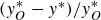 $(y^*_O - y^*) / y^*_O$
, where we achieve a good collapse of the amplitude modulation coefficient profiles. This successful scaling matches well with the AEH, where it is the distance to the reference location that affects
$(y^*_O - y^*) / y^*_O$
, where we achieve a good collapse of the amplitude modulation coefficient profiles. This successful scaling matches well with the AEH, where it is the distance to the reference location that affects
 $\varGamma$
where the number of attached eddies also correlates to the distance. This increases the robustness of the IOIM framework, where we no longer need to calibrate for an additional set of amplitude modulation coefficients when we vary the input location for turbulent flow with the same flow parameters, which is often the most computationally costly process due to the iterative nature of finding
$\varGamma$
where the number of attached eddies also correlates to the distance. This increases the robustness of the IOIM framework, where we no longer need to calibrate for an additional set of amplitude modulation coefficients when we vary the input location for turbulent flow with the same flow parameters, which is often the most computationally costly process due to the iterative nature of finding
 $\varGamma$
. We must note that the difference in amplitude modulation coefficients is inconsequential when
$\varGamma$
. We must note that the difference in amplitude modulation coefficients is inconsequential when
 $(y^*_O - y^*) / y^*_O$
is small, i.e. close to the known signal. The logarithmic scale axis exaggerates the differences, where they are of order
$(y^*_O - y^*) / y^*_O$
is small, i.e. close to the known signal. The logarithmic scale axis exaggerates the differences, where they are of order
 $10^{-3}$
, which do not make a large difference for predictions in practice. Still, figure 26 further shows the strength of the IOIM framework, where even with different known locations for the same flow, we can make a credible prediction without finding another set of amplitude modulation coefficients given a known linear transfer kernel with the IOIM.
$10^{-3}$
, which do not make a large difference for predictions in practice. Still, figure 26 further shows the strength of the IOIM framework, where even with different known locations for the same flow, we can make a credible prediction without finding another set of amplitude modulation coefficients given a known linear transfer kernel with the IOIM.
Overall, given the relative universality of the universal signal and the collapse of the amplitude modulation coefficients, the IOIM displays high robustness across varying reference locations. While the linear transfer kernel profile does change with varying
 $y^*_O$
, the relative similarities across the other parameters illustrate the strengths of the IOIM framework even when the input is varied.
$y^*_O$
, the relative similarities across the other parameters illustrate the strengths of the IOIM framework even when the input is varied.
4.5. Constant reference location
In the previous section, § 4.4, we had varied the reference location,
 $y^*_O$
, for one flow case, where it exhibited significant variations in the linear transfer kernel profile and the amplitude modulation coefficients. In particular, the variation in the linear transfer kernel resembles the variation due to the Reynolds number effect observed previously. This naturally raises the question of whether the observed trends were manifested from the change in the outer reference location,
$y^*_O$
, for one flow case, where it exhibited significant variations in the linear transfer kernel profile and the amplitude modulation coefficients. In particular, the variation in the linear transfer kernel resembles the variation due to the Reynolds number effect observed previously. This naturally raises the question of whether the observed trends were manifested from the change in the outer reference location,
 $y_O^+ = 3.9 \textit{Re}_\tau ^{({1}/{2})}$
, rather than the Reynolds number. To further investigate the effect of the reference location on the IOIM and its parameters, in the following, we have fixed the reference location to be around
$y_O^+ = 3.9 \textit{Re}_\tau ^{({1}/{2})}$
, rather than the Reynolds number. To further investigate the effect of the reference location on the IOIM and its parameters, in the following, we have fixed the reference location to be around
 $y_O^* \approx 117.6$
, as shown in table 5.
$y_O^* \approx 117.6$
, as shown in table 5.
Cases with the outer reference location set to
 $y^*_{O, \textit{const.}} \approx 117.6$
with adjustments based on the DNS grid sizes. The cases are labelled with the subscript
$y^*_{O, \textit{const.}} \approx 117.6$
with adjustments based on the DNS grid sizes. The cases are labelled with the subscript
 $_{\textit{const.}}$
to indicate the difference, where the deviation indicates the percentage change from the original outer reference location based on the formulation
$_{\textit{const.}}$
to indicate the difference, where the deviation indicates the percentage change from the original outer reference location based on the formulation
 $y_O^* = 3.9 {\textit{Re}_\tau ^*}^{({1}/{2})}$
.
$y_O^* = 3.9 {\textit{Re}_\tau ^*}^{({1}/{2})}$
.

4.5.1. Linear transfer kernel –
$\widetilde {H}_L$

The linear transfer kernel magnitudes at the largest inner-scaled wavelengths for the cases with a constant reference location are shown in figure 27, where they exhibit increased similarity to one another, and the incompressible cases collapse to one another. Furthermore, the higher Reynolds number compressible flow cases, Ma08Re783
 $_{\textit{const.}}$
and Ma15Re773
$_{\textit{const.}}$
and Ma15Re773
 $_{\textit{const.}}$
, are also fairly close to the incompressible profiles, with compressibility decreasing their profiles slightly. The lower Reynolds number compressible flow cases, where the deviation from the standard reference location is the largest (
$_{\textit{const.}}$
, are also fairly close to the incompressible profiles, with compressibility decreasing their profiles slightly. The lower Reynolds number compressible flow cases, where the deviation from the standard reference location is the largest (
 $\sim 50\%$
), produce profiles with smaller magnitudes. Their relatively lower Reynolds number may be due to insufficient scale separation for a true comparison.
$\sim 50\%$
), produce profiles with smaller magnitudes. Their relatively lower Reynolds number may be due to insufficient scale separation for a true comparison.
The linear transfer kernel magnitudes at the largest inner-scaled wavelengths,
 ${\lambda _x^+}_{\textit{max}}$
, for the cases with a constant reference location.
${\lambda _x^+}_{\textit{max}}$
, for the cases with a constant reference location.

Any Reynolds number trend observed within the linear transfer kernel, particularly for the incompressible flow cases, can be readily removed through the use of a constant reference location linear transfer kernel. Compressibility effects, on the other hand, still seem rather difficult to quantify and remove specifically so that the profiles can be reverted to their incompressible counterparts.
4.5.2. Universal signal –
$u^*$

The universal signals for the cases in table 5 are then shown in the figure 28. The universal signals, compared with the detrended signals from the conventional reference location, shown in figures 9 and 11, show remarkable similarities for the premultipled energy spectra and display sufficient extraction of the small scales. We do note that some of the cases with the larger deviations from the standard reference location, i.e. Ma15Re394
 $_{\textit{const.}}$
around
$_{\textit{const.}}$
around
 $y^* = 3$
and Ma30Re396
$y^* = 3$
and Ma30Re396
 $_{\textit{const.}}$
around
$_{\textit{const.}}$
around
 $y^* = 9$
suffer slightly from numerical stability and their universal signals are not as refined. This may be due to insufficient scale separation combined with the fact that the deviation from the usual outer spectral peak reference location is fairly large. From this, when one chooses the outer reference location, one should not deviate from the typical
$y^* = 9$
suffer slightly from numerical stability and their universal signals are not as refined. This may be due to insufficient scale separation combined with the fact that the deviation from the usual outer spectral peak reference location is fairly large. From this, when one chooses the outer reference location, one should not deviate from the typical
 $y^*_O = 3.9 {Re^*_\tau }^{({1}/{2})}$
for the IOIM framework to perform up to its full capabilities. Figure 29 presents the one-dimensional premultiplied energy spectra, similar to figures 10 and 12, where we continue to find similarities between the small scales of incompressible and compressible flows. With a similar outer reference location, it is obvious that the previously observed similarities in proportion of energy that the universal signal takes up are very similar, even without the scaling of the outer reference location as seen in figure 29(a). In figure 29(b), we see that the previously observed trends follow a similar limit after the wall-normal coordinate scaling. The reference location has the least effect in general on the IOIM’s parameters, further suggesting the relative similarities between the small scales of the incompressible and compressible flows extracted from the IOIM framework.
$y^*_O = 3.9 {Re^*_\tau }^{({1}/{2})}$
for the IOIM framework to perform up to its full capabilities. Figure 29 presents the one-dimensional premultiplied energy spectra, similar to figures 10 and 12, where we continue to find similarities between the small scales of incompressible and compressible flows. With a similar outer reference location, it is obvious that the previously observed similarities in proportion of energy that the universal signal takes up are very similar, even without the scaling of the outer reference location as seen in figure 29(a). In figure 29(b), we see that the previously observed trends follow a similar limit after the wall-normal coordinate scaling. The reference location has the least effect in general on the IOIM’s parameters, further suggesting the relative similarities between the small scales of the incompressible and compressible flows extracted from the IOIM framework.
The universal signals premultiplied energy spectra,
 $k_x\phi _{u^*u^*}$
, for the cases with a constant reference location as listed in table 5: (a) Re547
$k_x\phi _{u^*u^*}$
, for the cases with a constant reference location as listed in table 5: (a) Re547
 $_{\textit{const.}}$
, (b) Re934
$_{\textit{const.}}$
, (b) Re934
 $_{\textit{const.}}$
, (c) Re2003
$_{\textit{const.}}$
, (c) Re2003
 $_{\textit{const.}}$
, (d) Ma08Re384
$_{\textit{const.}}$
, (d) Ma08Re384
 $_{\textit{const.}}$
, (e) Ma08Re783
$_{\textit{const.}}$
, (e) Ma08Re783
 $_{\textit{const.}}$
, (f) Ma15Re394
$_{\textit{const.}}$
, (f) Ma15Re394
 $_{\textit{const.}}$
, (g) Ma15Re773
$_{\textit{const.}}$
, (g) Ma15Re773
 $_{\textit{const.}}$
and (h) Ma30Re396
$_{\textit{const.}}$
and (h) Ma30Re396
 $_{\textit{const.}}$
, respectively.
$_{\textit{const.}}$
, respectively.

One-dimensional premultiplied energy spectra for the cases with constant reference locations (a) as a function of the wall-normal heights,
 $y^*$
, scaled by the total energies, and (b) as a function of scaled wall-normal heights,
$y^*$
, scaled by the total energies, and (b) as a function of scaled wall-normal heights,
 $y^* / y^*_O$
, also scaled by total energies. The dashed line is (4.2), where the parameters are again
$y^* / y^*_O$
, also scaled by total energies. The dashed line is (4.2), where the parameters are again
 $A = 0.99$
and
$A = 0.99$
and
 $B = 7.5$
, similar to figures 10(b) and 12(b).
$B = 7.5$
, similar to figures 10(b) and 12(b).

4.5.3. Amplitude modulation –
$\varGamma$

Lastly, the amplitude modulation coefficients are shown in figure 30. We observe that the compressible flows achieve a fairly similar
 $\varGamma$
profiles with a similar
$\varGamma$
profiles with a similar
 $y^*_O$
at
$y^*_O$
at
 ${\textit {Ma}}_b = 0.8$
and
${\textit {Ma}}_b = 0.8$
and
 $1.5$
despite the difference in Reynolds number, suggesting that the Reynolds number dependence of the amplitude modulation coefficients for the compressible flow cases can be readily removed. However, this cannot be achieved for the incompressible flow cases, raising questions regarding the collapse of profiles of the compressible cases. Furthermore, the Reynolds numbers for the incompressible flow cases are much greater than those of the compressible flow cases. The compressible flow
$1.5$
despite the difference in Reynolds number, suggesting that the Reynolds number dependence of the amplitude modulation coefficients for the compressible flow cases can be readily removed. However, this cannot be achieved for the incompressible flow cases, raising questions regarding the collapse of profiles of the compressible cases. Furthermore, the Reynolds numbers for the incompressible flow cases are much greater than those of the compressible flow cases. The compressible flow
 $\varGamma$
behaviour at higher Reynolds numbers, where a higher degree of large-scale influence is present, is unknown, so the current observed collapse of profiles may not be universal. The Re547
$\varGamma$
behaviour at higher Reynolds numbers, where a higher degree of large-scale influence is present, is unknown, so the current observed collapse of profiles may not be universal. The Re547
 $_{\textit{const.}}$
and Re934
$_{\textit{const.}}$
and Re934
 $_{\textit{const.}}$
amplitude modulation profiles, where their Reynolds number are more comparable to the compressible cases, are quite similar. Ultimately, it is generally advised to keep the outer reference location to the formulation of
$_{\textit{const.}}$
amplitude modulation profiles, where their Reynolds number are more comparable to the compressible cases, are quite similar. Ultimately, it is generally advised to keep the outer reference location to the formulation of
 $y^*_O = 3.9Re^{({1}/{2})}$
to avoid any numerical instabilities during scale separation, as seen in this and the previous sections, where its effects on the IOIM parameters cannot be readily quantified.
$y^*_O = 3.9Re^{({1}/{2})}$
to avoid any numerical instabilities during scale separation, as seen in this and the previous sections, where its effects on the IOIM parameters cannot be readily quantified.
Amplitude modulation profiles for the cases with constant reference locations from table 5.

4.6. Compressibility and density variation considerations
Outside of the IOIM’s parameters, one aspect that hinders the IOIM’s universality is the scaling of compressible velocity fluctuations as described at the beginning of § 4. Throughout this study, we have used density-weighted velocity fluctuations,
 $\sqrt {\rho }u''$
, in an attempt to account for the density variations within the compressible flow cases. Even at subsonic ranges, we can observe significant compressibility effects, where behaviours of
$\sqrt {\rho }u''$
, in an attempt to account for the density variations within the compressible flow cases. Even at subsonic ranges, we can observe significant compressibility effects, where behaviours of
 $\varGamma$
and
$\varGamma$
and
 $\widetilde {H}_L$
differ significantly from their incompressible equivalents. As compressibility increases, and correspondingly density variations increase, the separation between the incompressible IOIM parameters and the compressible IOIM parameters increases. While small-scale motions have a high degree of similarity across the two flow regimes, as evidenced by the strong likenesses of
$\widetilde {H}_L$
differ significantly from their incompressible equivalents. As compressibility increases, and correspondingly density variations increase, the separation between the incompressible IOIM parameters and the compressible IOIM parameters increases. While small-scale motions have a high degree of similarity across the two flow regimes, as evidenced by the strong likenesses of
 $u^*$
, the parameters which directly involve LSMs and their effects also exhibit greater differences. Furthermore, we have deployed semilocal scaling for all the compressible flow cases, since it has long been shown to be the most effective wall-normal scaling (Trettel & Larsson Reference Trettel and Larsson2016). For a thorough investigation, we have also independently investigated the use of inner- and outer-scaling on the effects of compressibility to holistically evaluate different scalings, but nevertheless, we have verified that the current conclusions are not affected by different scaling, where the same
$u^*$
, the parameters which directly involve LSMs and their effects also exhibit greater differences. Furthermore, we have deployed semilocal scaling for all the compressible flow cases, since it has long been shown to be the most effective wall-normal scaling (Trettel & Larsson Reference Trettel and Larsson2016). For a thorough investigation, we have also independently investigated the use of inner- and outer-scaling on the effects of compressibility to holistically evaluate different scalings, but nevertheless, we have verified that the current conclusions are not affected by different scaling, where the same
 ${\textit {Ma}}_b$
effects are observed. Semilocal scaling remains the most suitable, especially when compared with cases within the incompressible flow regime.
${\textit {Ma}}_b$
effects are observed. Semilocal scaling remains the most suitable, especially when compared with cases within the incompressible flow regime.
Ultimately, one of the possible reasons for non-universality can be traced back to the
 $\sqrt {\rho }u''$
scaling of the velocity fluctuations, where, within the IOIM framework, it cannot suitably account for the density variations fully. While this topic extends far beyond the scope of not only the IOIM, the scaling of compressible velocity fluctuations remains vital work and has significant room for improvement. This scaling seems to deviate as
$\sqrt {\rho }u''$
scaling of the velocity fluctuations, where, within the IOIM framework, it cannot suitably account for the density variations fully. While this topic extends far beyond the scope of not only the IOIM, the scaling of compressible velocity fluctuations remains vital work and has significant room for improvement. This scaling seems to deviate as
 ${\textit {Ma}}_b$
increases (Huang et al. Reference Huang, Duan and Choudhanri2022), leading to previous deviations in predictions of the incompressible fluctuations when using higher
${\textit {Ma}}_b$
increases (Huang et al. Reference Huang, Duan and Choudhanri2022), leading to previous deviations in predictions of the incompressible fluctuations when using higher
 ${\textit {Ma}}_b$
universal signals in § 4.2. Suitable scaling may impart the potential to unite the IOIM parameters across incompressible and compressible flows, and it will, of course, have crucial consequences for greater universality arguments in general. Within this study, we have seen that with the current scaling, as compressibility increases, the parameters are generally dampened. Future scaling will need to ‘push’ these parameter values ‘up’, which may help recover the incompressible IOIM parameter trends.
${\textit {Ma}}_b$
universal signals in § 4.2. Suitable scaling may impart the potential to unite the IOIM parameters across incompressible and compressible flows, and it will, of course, have crucial consequences for greater universality arguments in general. Within this study, we have seen that with the current scaling, as compressibility increases, the parameters are generally dampened. Future scaling will need to ‘push’ these parameter values ‘up’, which may help recover the incompressible IOIM parameter trends.
5. Concluding remarks
We have applied the IOIM framework to a wide range of canonical wall-bounded turbulence flows across incompressible and compressible regimes. The parameters for the cases with varying Mach (
 $0.8 \leqslant {\textit {Ma}}_b \leqslant 3$
) and Reynolds numbers (
$0.8 \leqslant {\textit {Ma}}_b \leqslant 3$
) and Reynolds numbers (
 $140 \leqslant \textit{Re}_\tau ^* \leqslant 2003$
) have been scrutinised to observe trends, if any, which have been quantified by empirical means. While previous studies suggest that the IOIM’s parameters are universal, we found that most of its parameters exhibit large variations with respect to the flow parameters. The IOIM framework was initially designed to capture large-scale effects and their relationship with small scales via the amplitude modulation mechanism, where a sufficiently large Reynolds number is needed (
$140 \leqslant \textit{Re}_\tau ^* \leqslant 2003$
) have been scrutinised to observe trends, if any, which have been quantified by empirical means. While previous studies suggest that the IOIM’s parameters are universal, we found that most of its parameters exhibit large variations with respect to the flow parameters. The IOIM framework was initially designed to capture large-scale effects and their relationship with small scales via the amplitude modulation mechanism, where a sufficiently large Reynolds number is needed (
 $\textit{Re}_\tau \approx 2000$
). However, the framework is still numerically capable of capturing the mechanisms involved at lower
$\textit{Re}_\tau \approx 2000$
). However, the framework is still numerically capable of capturing the mechanisms involved at lower
 $\textit{Re}_\tau$
and despite the introduction of compressibility.
$\textit{Re}_\tau$
and despite the introduction of compressibility.
We also provided connections between AEH and the IOIM framework’s parameters. From this perspective, one can view the amplitude modulation coefficient as the relative strength of the VLSMs, LSMs and attached eddies, and as we near the wall, the viscous-dominated near-wall eddies come into play as well, affecting the amplitude modulation coefficient. The
 $\varGamma$
profiles, which seem to be rooted in empirical means, can be explained through the aforementioned physical structures, compensating for the changes caused by the varying presence of different eddies and the decreasing large-scale coherent signal
$\varGamma$
profiles, which seem to be rooted in empirical means, can be explained through the aforementioned physical structures, compensating for the changes caused by the varying presence of different eddies and the decreasing large-scale coherent signal
 $u_S^+$
. With the introduction of compressibility, this profile exhibits further variation, which weakens the amplitude modulation mechanism as
$u_S^+$
. With the introduction of compressibility, this profile exhibits further variation, which weakens the amplitude modulation mechanism as
 ${\textit {Ma}}_b$
increases. However, no distinct connections between the incompressible and compressible
${\textit {Ma}}_b$
increases. However, no distinct connections between the incompressible and compressible
 $\varGamma$
profiles have been found, and further investigation on the amplitude modulation mechanism, or from our alternative perspective, the balance between different turbulence structures, between the two flow regimes, should be conducted. The differences in amplitude modulation mechanism between the incompressible and compressible flow cases also pose a challenge to Morkorvin’s assertion in 1962 that ‘the essential dynamics of these supersonic shear flows will follow the incompressible pattern’ (Bross et al. Reference Bross, Scharnowski and Kähler2021). The amplitude modulation mechanism is one of the universal mechanisms in wall-bounded turbulence, yet it still exhibits distinctly different
$\varGamma$
profiles have been found, and further investigation on the amplitude modulation mechanism, or from our alternative perspective, the balance between different turbulence structures, between the two flow regimes, should be conducted. The differences in amplitude modulation mechanism between the incompressible and compressible flow cases also pose a challenge to Morkorvin’s assertion in 1962 that ‘the essential dynamics of these supersonic shear flows will follow the incompressible pattern’ (Bross et al. Reference Bross, Scharnowski and Kähler2021). The amplitude modulation mechanism is one of the universal mechanisms in wall-bounded turbulence, yet it still exhibits distinctly different
 $\varGamma$
profiles, where we can assert strong intrinsic compressibility effects which differentiate incompressible and compressible flow. The study on the variation of the known reference location,
$\varGamma$
profiles, where we can assert strong intrinsic compressibility effects which differentiate incompressible and compressible flow. The study on the variation of the known reference location,
 $y_O^+$
, further strengthens the physical perspective we provided in § 2.2, where
$y_O^+$
, further strengthens the physical perspective we provided in § 2.2, where
 $\varGamma$
increases as
$\varGamma$
increases as
 $y_O^+$
increases to compensate for the increase in eddies as we near the wall. A collapse of
$y_O^+$
increases to compensate for the increase in eddies as we near the wall. A collapse of
 $\varGamma$
profiles with different
$\varGamma$
profiles with different
 $y_O^+$
based on a normalisation from distance from
$y_O^+$
based on a normalisation from distance from
 $y_O^+$
reinforces this physical viewpoint as well.
$y_O^+$
reinforces this physical viewpoint as well.
The linear transfer kernel also exhibits the effects of compressibility, where it decreases the energy transfer in the wall-normal direction, which agrees well with other independent studies on compressibility effects and their dampening on energy transfer. Across any shared inner-scaled streamwise wavelengths, it was also found that the lower Reynolds number flow has a larger proportion of the superposition signal. While previous studies suggest that
 $\widetilde {H}_L$
is universal based on visual assessment, this study highlights the quantitative differences between the profiles as flow parameters vary, where compressibility effects can be observed.
$\widetilde {H}_L$
is universal based on visual assessment, this study highlights the quantitative differences between the profiles as flow parameters vary, where compressibility effects can be observed.
From the universal signal, we find that the near-wall dynamics across the compressible and incompressible flow regimes possess a high degree of similarity. Adjusting and normalising for the total energy of the flow, it is found that the universal signal occupies a similar proportion of the total energy across incompressible and compressible flows, as observed through (4.2). Even as we move from subsonic to supersonic ranges, the universal signal still follows this empirical relation rather well. Their PDFs also hold relative similarities, especially within the near-wall region, further reinforcing the image and links between the IOIM’s universal signal and the viscous-dominated near-wall detached eddies. This notion of the universality of the small scales has long been established, where the natural decomposition based on SLSE of large and small scales is somewhat effective and robust, as seen with the prediction of incompressible flow cases using the universal signals calibrated from compressible flow cases.
In this study, while empirical trends were captured with the available data, as described before, due to limits in computational resources, a wider range of Reynolds numbers and Mach numbers DNS data was not available. High Reynolds number data allows for improved scale separation and significant VLSM effects, where the IOIM and AEM work best. It is pertinent to continue this study at higher Reynolds numbers, where a further investigation into the IOIM parameters will be even more meaningful with regard to universality. The low to medium Reynolds number data used here prevents a completely holistic non-universal argument throughout the entire flow regimes, but still provides a basis as to the advantages and disadvantages of the IOIM framework. To further validate the relationships found, the IOIM framework must be applied to data at higher Reynolds and Mach numbers, which will be further beneficial for the study of the robustness of the IOIM framework and its parameters. Furthermore, the Mach number effect has not yet been empirically captured within this study, especially with regard to the amplitude modulation coefficients, and remains vital work to further enhance the universality of the IOIM framework. Still, the IOIM framework in its current state exhibits significant variations in its parameters across incompressible and compressible flow, and will need further modifications to bring a unified framework across the two flow regimes.
Acknowledgements
The authors are grateful for the data provided by Baars (Reference Baars2020).
Funding
This work was supported by the National Natural Science Foundation of China (no. 12422210). J.E.K.I.S. gratefully acknowledges the Hong Kong PhD Fellowship Scheme funded by the Research Grants Council (RGC) of the Hong Kong Special Administrative Region (HKSAR) Government (no. PF22-79233). L.F. also acknowledges the funding from the RGC of the HKSAR Government with RGC/ECS Project (no. 26200222), RGC/GRF Project (no. 16201023), RGC/STG Project (no. STG2/E-605/23-N), RGC/TRS Project (no. T22-607/24N), and the funding from Guangdong Basic and Applied Basic Research Foundation (no. 2024A1515011798).
Declaration of interests
The authors report no conflict of interest.
Data availability statement
The data within this paper is available upon request.
The unfiltered linear transfer kernel profiles for the incompressible flow cases as listed in table 1, i.e. before the BMF operation, enforcement of roll-off to zero at smaller wavelengths and scaling of transfer gains at the largest wavelengths to be unity.

The unfiltered linear transfer kernel profiles for the compressible flow cases as listed in table 2, i.e. before the BMF operation, enforcement of roll-off to zero at smaller wavelengths and scaling of transfer gains at the largest wavelengths to be unity.

Appendix A. Effects of the domain sizes on the linear transfer kernel
$\widetilde {H}_L$

The readers may notice that the linear transfer kernels possess some humps and inflections at the larger wall-normal coordinates and at the smaller wavelengths, which are more apparent in the compressible flow cases as seen in figure 5. When compared with the linear transfer kernels in the incompressible flow cases, these humps and inflections are not as evident, and some may ponder whether this may be an additional consequence of the introduction of compressibility, and we had hoped to clarify this point and not mislead the readers.
These observed humps and inflections arise mainly due to the numerical averaging operation by the
 $\pm 25\,\%$
BMF, which enforces a roll-off to zero upon a sufficiently small wavelength, combined with the inconsistent gain factors at the smaller wavelengths and scaling of the gains at the largest wavelengths to be unity. Some of the incoherent fluctuations propagate into the conditional output, as described by Baars et al. (Reference Baars, Hutchins and Marusic2016), creeping in at the lower wavelengths, which can be seen in the unfiltered linear transfer kernels. Figures 31 and 32 show the unfiltered (or raw) linear transfer kernels for the incompressible and compressible flow cases, respectively. Due to limitations in the streamwise domain for the compressible flow cases, the roll-off to zero is sometimes not complete, leading to these somewhat awkward points of inflections of bumps. While they do not have an effect on the overall framework of the IOIM, we believe a larger streamwise domain would resolve this issue, and that these points do not have any physical meaning. Most of the incompressible flow cases have a larger streamwise domain than their compressible counterparts; hence, these points are more apparent in the compressible cases. In the Re2003 incompressible flow case, we do observe a small hump as seen in the compressible cases, but this is since its streamwise domain,
$\pm 25\,\%$
BMF, which enforces a roll-off to zero upon a sufficiently small wavelength, combined with the inconsistent gain factors at the smaller wavelengths and scaling of the gains at the largest wavelengths to be unity. Some of the incoherent fluctuations propagate into the conditional output, as described by Baars et al. (Reference Baars, Hutchins and Marusic2016), creeping in at the lower wavelengths, which can be seen in the unfiltered linear transfer kernels. Figures 31 and 32 show the unfiltered (or raw) linear transfer kernels for the incompressible and compressible flow cases, respectively. Due to limitations in the streamwise domain for the compressible flow cases, the roll-off to zero is sometimes not complete, leading to these somewhat awkward points of inflections of bumps. While they do not have an effect on the overall framework of the IOIM, we believe a larger streamwise domain would resolve this issue, and that these points do not have any physical meaning. Most of the incompressible flow cases have a larger streamwise domain than their compressible counterparts; hence, these points are more apparent in the compressible cases. In the Re2003 incompressible flow case, we do observe a small hump as seen in the compressible cases, but this is since its streamwise domain,
 $4\pi h$
, is smaller than the other incompressible cases, yet it is also the same as the compressible flow cases, suggesting the domain size as the cause for this phenomenon. It is recommended for future users of the IOIM framework that, if possible, a larger domain size is utilised for employing the IOIM to avoid these numerical issues.
$4\pi h$
, is smaller than the other incompressible cases, yet it is also the same as the compressible flow cases, suggesting the domain size as the cause for this phenomenon. It is recommended for future users of the IOIM framework that, if possible, a larger domain size is utilised for employing the IOIM to avoid these numerical issues.


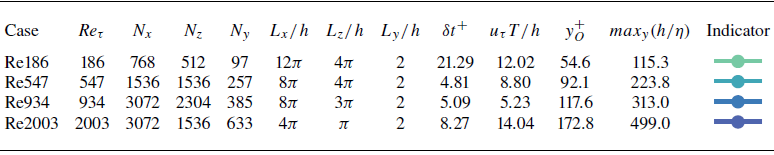


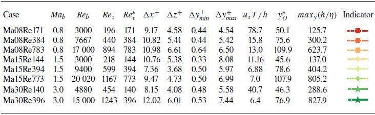


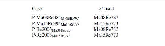


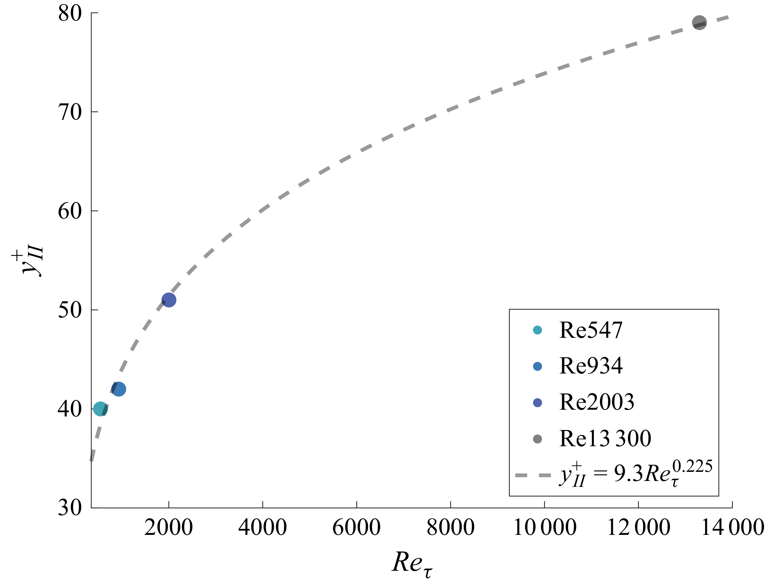


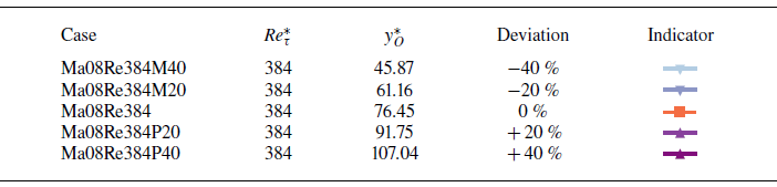


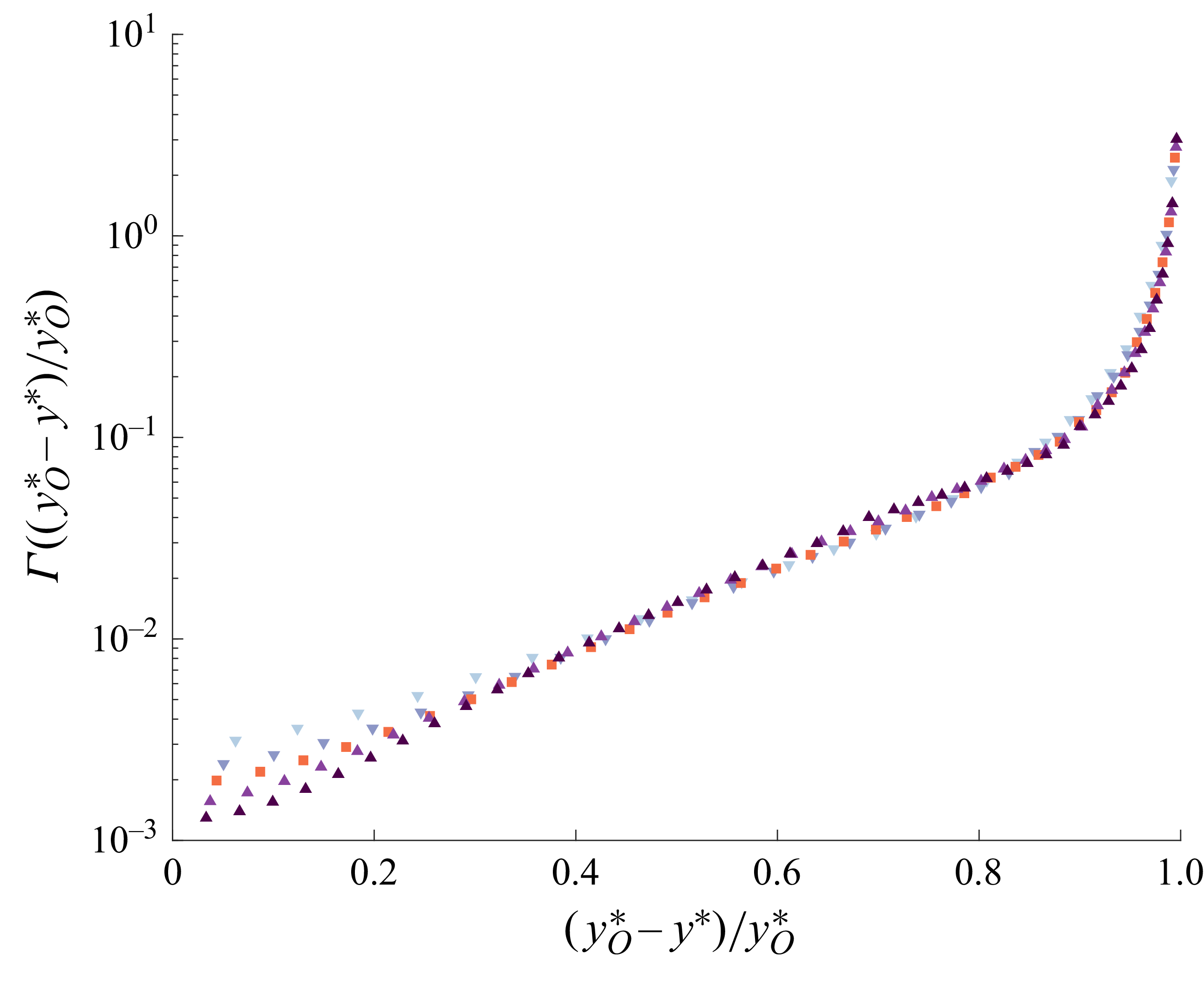


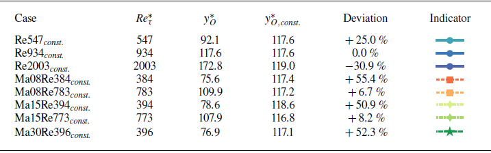


 Open access