


1. Introduction
The analytic solution for axisymmetric incompressible potential flows over cones in infinite domain is well documented in the literature (Whitehead & Canetti Reference Whitehead and Canetti1950; Rosenhead Reference Rosenhead1988). Axisymmetric compressible flows over cones are described by the Taylor–Maccoll equations, which require numerical solution of the system of differential equations (Taylor & Maccoll Reference Taylor and Maccoll1933; Maccoll Reference Maccoll1937). Loss of axisymmetry at incidence has so far precluded analytic description of the flows. At increasing angles of incidence, flow separation regions emerge at the leeward surface of the cones. These separation regions essentially comprise the rolled up vorticity of the boundary layers. The vortex systems over non-spinning cones are symmetric; hence, the resulting lateral forces are neutralised and the flows are typically favourable. However, at sufficiently high angles of incidence, the vortex systems destabilise, lose their symmetry and exhibit adverse effects. Ericsson & Reding (Reference Ericsson and Reding1985) examine the disparity between experimental and theoretical flows stemming from the asymmetric vortex systems of slender bodies.
Flows over a variety of axisymmetric models at angles of incidence are visualised with exceptional quality in the ONERA water tunnel, where fine details of trailing vortex systems are made visible (Werle Reference Werle1979; Van Dyke Reference Van Dyke1982). Flows are visualised over two cones with a diameter-based Reynolds number between 4000 and 6000: a $\theta _c=5^\circ$
half-angle cone at
$\theta _c=5^\circ$
half-angle cone at $\alpha =5^\circ$
and
$\alpha =5^\circ$
and $20^\circ$
angles of incidence, and a
$20^\circ$
angles of incidence, and a $\theta _c=12.5^\circ$
half-angle cone at
$\theta _c=12.5^\circ$
half-angle cone at $10^\circ$
and
$10^\circ$
and $20^\circ$
angles of incidence. In each case, dye is injected from small ports on the cone surfaces, where the formations of symmetric trailing vortices are visible in the largest angle of incidence cases. The topology of the vortex systems is revealed in planes intersecting them, where distinction between primary and secondary vortices is made.
$20^\circ$
angles of incidence. In each case, dye is injected from small ports on the cone surfaces, where the formations of symmetric trailing vortices are visible in the largest angle of incidence cases. The topology of the vortex systems is revealed in planes intersecting them, where distinction between primary and secondary vortices is made.
Kumar, Guha & Kumar (Reference Kumar, Guha and Kumar2020) experimentally studied the trailing vortices behind a cone-cylinder body with a $\theta _c=12^\circ$
half-angle cone at
$\theta _c=12^\circ$
half-angle cone at $\alpha =40^\circ$
and a diameter-based Reynolds number of
$\alpha =40^\circ$
and a diameter-based Reynolds number of $1.3 \times 10^5$
. In cross-sections normal to the cone surface, a symmetric pair of vortex triads consisting of primary, secondary and tertiary vortices are visualised in vorticity contours extracted from planar particle image velocimetry (PIV) measurements. Asymmetries past the cone and cylindrical body junction ensue in the trailing vortex system.
$1.3 \times 10^5$
. In cross-sections normal to the cone surface, a symmetric pair of vortex triads consisting of primary, secondary and tertiary vortices are visualised in vorticity contours extracted from planar particle image velocimetry (PIV) measurements. Asymmetries past the cone and cylindrical body junction ensue in the trailing vortex system.
The trailing vortex systems over spinning cones at angles of incidence are asymmetric, owing to the centrifugal and viscous effects of rotation. Kuraan & Savaş (2020) visualised the flows over a $\theta _c=30^\circ$
half-angle cone, spinning with a rotational speed ratio at the base of approximately 3, a diameter-based Reynolds number of approximately
$\theta _c=30^\circ$
half-angle cone, spinning with a rotational speed ratio at the base of approximately 3, a diameter-based Reynolds number of approximately $10^4$
, and over a range of angles of incidence between 0
$10^4$
, and over a range of angles of incidence between 0 $^\circ$
and
$^\circ$
and $36^\circ$
using a smoke-wire technique. The streakline patterns reveal increasing asymmetries with increasing angles of incidence. For spinning cases, streaklines near the cone surface are shaped in the direction of rotation. Signatures of trailing vortex systems near the leeward surface of the cone are present at angles of incidence greater than
$36^\circ$
using a smoke-wire technique. The streakline patterns reveal increasing asymmetries with increasing angles of incidence. For spinning cases, streaklines near the cone surface are shaped in the direction of rotation. Signatures of trailing vortex systems near the leeward surface of the cone are present at angles of incidence greater than $18^\circ$
.
$18^\circ$
.
Several studies focus on boundary layer instabilities over non-spinning and spinning cones at zero incidence (Illingworth Reference Illingworth1953; Tien & Tsuji Reference Tien and Tsuji1965; Kobayashi Reference Kobayashi1981; Kobayashi, Kohama & Kurosawa Reference Kobayashi, Kohama and Kurosawa1983; Garrett & Peake Reference Garrett and Peake2007; Hussain et al. Reference Hussain, Stephen and Garrett2012, Reference Hussain, Garrett and Stephen2014, Reference Hussain, Garrett, Stephen and Griffiths2016; Tambe et al. Reference Tambe, Schrijer, Veldhuis and Rao2022). Recently, Alfredsson, Kentaro & Lingwood (Reference Alfredsson, Kentaro and Lingwood2024) presented an extensive review of instability, transition and turbulence in the boundary layer flows over spinning cones and discs in infinite still fluid. They remark that, however, ’there are adjacent interesting flows that are less studied, such as a coflowing surrounding fluid, with or without angle of attack’.
Limited studies focus on the effects of angles of incidence (Adams Reference Adams1972; Schneider Reference Schneider2004; Tambe et al. Reference Tambe, Schrijer and Veldhuis2021). Nevertheless, the range of angles of incidence is limited to angles less than the half-angle of the cone, where trailing vortex systems have not yet developed. Studies addressing asymmetries of flows over spinning cones at angles of incidence are confined to boundary layer regions, whereas the effects of rotation on trailing vortex systems are sparse. Previous flow visualisation experiments have provided steady reference flows over a range of half-angle cones spinning in uniform non-axial flows; however, no works comprehensively quantify the induced asymmetric vortical flows. Kuraan & Savaş (2020) provide steady reference flows over a spinning cone with a $30^\circ$
half-angle over a range of incidence angles, which serve as motivation for the present more comprehensive work.
$30^\circ$
half-angle over a range of incidence angles, which serve as motivation for the present more comprehensive work.
The present study aims to characterise the influences of angle of incidence, the cone half-angle and the rotational speed parameter on low-speed, incompressible viscous flows over spinning cones at angles of incidence. Flows across five cones with half-angles $\theta _c = 10^\circ$
,
$\theta _c = 10^\circ$
, $15^\circ$
,
$15^\circ$
, $22.5^\circ$
,
$22.5^\circ$
, $30^\circ$
and
$30^\circ$
and $45^\circ$
are studied over a range of incidence angles,
$45^\circ$
are studied over a range of incidence angles, $0\leqslant \alpha \leqslant 36^\circ$
, at a free stream velocity of
$0\leqslant \alpha \leqslant 36^\circ$
, at a free stream velocity of $U_\infty =2$
m s−1 and constant angular speeds,
$U_\infty =2$
m s−1 and constant angular speeds, $\varOmega$
. The flows are characterised by Reynolds numbers that are
$\varOmega$
. The flows are characterised by Reynolds numbers that are $\mathcal O(10^4)$
and a range of rotational speed parameters at the base of each cone model of
$\mathcal O(10^4)$
and a range of rotational speed parameters at the base of each cone model of $0 \leqslant |S_D| \leqslant 3$
.
$0 \leqslant |S_D| \leqslant 3$
.
Definitions and parameters are introduced in § 2. Incompressible potential flow solutions over cones at zero incidence are reviewed in § 3. The smoke-wire and planar PIV experimental set-ups and procedures are described in § 4. Results and observations from the smoke visualisation experiment and planar PIV measurements are summarised in §§ 5–9 that comprise in-depth analyses of the experiments corresponding to $\theta _c = 10^\circ$
,
$\theta _c = 10^\circ$
, $15^\circ$
,
$15^\circ$
, $22.5^\circ$
,
$22.5^\circ$
, $30^\circ$
and
$30^\circ$
and $45^\circ$
cone models, respectively. Streaklines from the smoke visualisation experiments and streamlines computed from the PIV measurements at zero incidence are compared with incompressible potential flow streamlines to gauge the success of the experiments in each section. Closing remarks and conjectures are presented in § 10. The text is filled with smoke streakline images and contour plots deduced from PIV measurements. Extensive image sequences are presented as galleries throughout the text for each cone. To observe the intricate details of the streakline patterns, the reader may wish to study the individual images at sufficient magnification.
$45^\circ$
cone models, respectively. Streaklines from the smoke visualisation experiments and streamlines computed from the PIV measurements at zero incidence are compared with incompressible potential flow streamlines to gauge the success of the experiments in each section. Closing remarks and conjectures are presented in § 10. The text is filled with smoke streakline images and contour plots deduced from PIV measurements. Extensive image sequences are presented as galleries throughout the text for each cone. To observe the intricate details of the streakline patterns, the reader may wish to study the individual images at sufficient magnification.
2. Definitions and flow parameters
A schematic defining the geometry of a cone with a half-angle $\theta _c$
, its pertinent coordinate systems and the main flow parameters is shown in figure 1. The free stream flow
$\theta _c$
, its pertinent coordinate systems and the main flow parameters is shown in figure 1. The free stream flow $U_\infty$
is at angle of incidence
$U_\infty$
is at angle of incidence $\alpha$
with respect to the centreline of the cone. The cone spins at a constant angular speed
$\alpha$
with respect to the centreline of the cone. The cone spins at a constant angular speed $\varOmega$
. The windward surface corresponds to the surface of the cone that is directly exposed to the incoming free stream, and the leeward surface to the surface in the wake region downstream. Furthermore, section A–A in figure 1 shows a planar cross-section normal to the axis of the cone viewed from behind the cone, where the projected free stream component
$\varOmega$
. The windward surface corresponds to the surface of the cone that is directly exposed to the incoming free stream, and the leeward surface to the surface in the wake region downstream. Furthermore, section A–A in figure 1 shows a planar cross-section normal to the axis of the cone viewed from behind the cone, where the projected free stream component $U_\infty \sin \alpha$
is used in defining the co-rotating and counter-rotating meridians. The co-rotating meridian corresponds to the surface of the cone that rotates in the same direction as the incoming free stream component, whereas the counter-rotating meridian corresponds to the surface of the cone that rotates in the opposite direction as the incoming free stream. The component of the free stream velocity,
$U_\infty \sin \alpha$
is used in defining the co-rotating and counter-rotating meridians. The co-rotating meridian corresponds to the surface of the cone that rotates in the same direction as the incoming free stream component, whereas the counter-rotating meridian corresponds to the surface of the cone that rotates in the opposite direction as the incoming free stream. The component of the free stream velocity, $U_\infty \sin \alpha$
, will be frequently referred to as co-flow or counter-flow when discussing flows of co- and counter-rotating meridians, respectively. The term ’cross-flow’ is used when referring to three-dimensional boundary layer instabilities.
$U_\infty \sin \alpha$
, will be frequently referred to as co-flow or counter-flow when discussing flows of co- and counter-rotating meridians, respectively. The term ’cross-flow’ is used when referring to three-dimensional boundary layer instabilities.
Definitions: coordinate systems $(x,y,z), \ (x_*, y_*, z_*), \ (r, \theta , \phi )$
; cone dimensions
$(x,y,z), \ (x_*, y_*, z_*), \ (r, \theta , \phi )$
; cone dimensions $(D,H,L,\theta _c)$
, flow parameters
$(D,H,L,\theta _c)$
, flow parameters $(U_\infty , \varOmega , \alpha )$
and projected free stream component
$(U_\infty , \varOmega , \alpha )$
and projected free stream component $U_\infty \sin \alpha$
.
$U_\infty \sin \alpha$
.

The origins of all coordinate systems are fixed to the vertex of the cone. A fixed Cartesian coordinate system, ( $x, y, z$
), is defined with respect to the wind tunnel, where the
$x, y, z$
), is defined with respect to the wind tunnel, where the $x$
-axis is aligned with the centreline of the wind tunnel and positive in the downstream direction. Looking upstream from behind the cone, the
$x$
-axis is aligned with the centreline of the wind tunnel and positive in the downstream direction. Looking upstream from behind the cone, the $y$
-axis is defined positive to the right and the
$y$
-axis is defined positive to the right and the $z$
-axis positive up. A surface-aligned Cartesian coordinate system, (
$z$
-axis positive up. A surface-aligned Cartesian coordinate system, ( $x_*, y_*, z_*$
), is defined with respect to the generator of the cone. The velocity vectors corresponding to the wind tunnel and surface-aligned Cartesian coordinate systems,
$x_*, y_*, z_*$
), is defined with respect to the generator of the cone. The velocity vectors corresponding to the wind tunnel and surface-aligned Cartesian coordinate systems, $\boldsymbol{u}$
and
$\boldsymbol{u}$
and $\boldsymbol{u_*}$
, are defined in (2.1) and (2.2), respectively. Note that the surface-aligned Cartesian coordinate system is used to define wall-parallel,
$\boldsymbol{u_*}$
, are defined in (2.1) and (2.2), respectively. Note that the surface-aligned Cartesian coordinate system is used to define wall-parallel, $u_{||}$
, and wall-normal,
$u_{||}$
, and wall-normal, $u_\perp$
, velocities in the
$u_\perp$
, velocities in the $x_*$
and
$x_*$
and $z_*$
directions, respectively,
$z_*$
directions, respectively,
 \begin{equation} \boldsymbol{u}(x,y,z) = (u, v, w) \end{equation}
and
 \begin{equation} \boldsymbol{u_*}(x_*,y_*,z_*)= (u_*, v_*, w_*) = (u_{||}, v_*, u_\perp )\ . \end{equation}
Finally, a cone-attached spherical polar coordinate system, ( $r, \theta , \phi$
), is defined, where the polar axis is aligned with the cone centreline and the generator of the cone is marked by the polar half-angle of the cone,
$r, \theta , \phi$
), is defined, where the polar axis is aligned with the cone centreline and the generator of the cone is marked by the polar half-angle of the cone, $\theta _c$
. The spherical polar coordinates system is used in the incompressible axisymmetric potential flow solution over a cone. The velocity vector in spherical polar coordinates is defined as
$\theta _c$
. The spherical polar coordinates system is used in the incompressible axisymmetric potential flow solution over a cone. The velocity vector in spherical polar coordinates is defined as
 \begin{equation} \boldsymbol{u}(r,\theta ,\phi ) = (u_r, u_\theta , u_\phi ) \ . \end{equation}
The vorticity vector is defined with respect to the fixed wind tunnel Cartesian coordinate system as
 \begin{equation} \boldsymbol{\omega }(x,y,z) = (\omega _x, \omega _y, \omega _z) = \boldsymbol{\nabla }\times \boldsymbol{u}(x,y,z) \ . \end{equation}
The projection of the filament strength on the the $yz$
-plane is determined by integrating
$yz$
-plane is determined by integrating $\omega _x$
over the region of the vortex filament
$\omega _x$
over the region of the vortex filament
 \begin{equation} \varGamma = \sum _{i=1}^N \omega _{x,i} A_i, \end{equation}
where $A_i$
is the area subtended on the measurement grid by the local vorticity component
$A_i$
is the area subtended on the measurement grid by the local vorticity component $\omega _{x,i}$
.
$\omega _{x,i}$
.
Two Reynolds numbers are useful when describing the experiments with respect to dimensions of the cone models: the Reynolds number based on the base diameter $D$
of the cone and the inflow Reynolds number based on the length of the cone generator
$D$
of the cone and the inflow Reynolds number based on the length of the cone generator $L$
,
$L$
,
 \begin{equation} {\textit{Re}}_D = \frac {U_\infty D}{\nu } \end{equation}
and
 \begin{equation} {\textit{Re}}_L = \frac {U_\infty L}{\nu }, \end{equation}
where $D$
is the base diameter of the cone,
$D$
is the base diameter of the cone, $L = D/(2 \sin \theta _c)$
is the total length of the cone models along the
$L = D/(2 \sin \theta _c)$
is the total length of the cone models along the $x_*$
-axis and
$x_*$
-axis and $\nu$
is the kinematic viscosity of air. A third Reynolds number is based on vortex strength along the
$\nu$
is the kinematic viscosity of air. A third Reynolds number is based on vortex strength along the $x$
-axis,
$x$
-axis, $\varGamma$
, and is defined as
$\varGamma$
, and is defined as
 \begin{equation} {\textit{Re}}_{\varGamma } = \frac {\varGamma }{\nu }. \end{equation}
Here, ${\textit{Re}}_\varGamma$
is useful in quantification of the trailing vortices over cones at angles of incidence.
${\textit{Re}}_\varGamma$
is useful in quantification of the trailing vortices over cones at angles of incidence.
The influence of rotation is characterised by the rotational speed parameter at the base, $S_D$
, which is defined as
$S_D$
, which is defined as
 \begin{equation} S_D=\frac {\varOmega D/2}{U_\infty }. \end{equation}
Essentially, $S_D$
is a ratio of the peripheral velocity at the base of the cone and the incoming free stream velocity. Here,
$S_D$
is a ratio of the peripheral velocity at the base of the cone and the incoming free stream velocity. Here, $S_D$
and
$S_D$
and ${\textit{Re}}_D$
are used as a convenient way to describe the experimental conditions; however, they are analogous to the local governing parameters used to characterise the laminar–turbulent boundary layer transition over spinning cones,
${\textit{Re}}_D$
are used as a convenient way to describe the experimental conditions; however, they are analogous to the local governing parameters used to characterise the laminar–turbulent boundary layer transition over spinning cones, ${\textit{Re}}_l=u_e l / \nu$
and
${\textit{Re}}_l=u_e l / \nu$
and $S=\varOmega r/u_e$
, where
$S=\varOmega r/u_e$
, where $u_e$
is the boundary layer edge velocity,
$u_e$
is the boundary layer edge velocity, $l$
is the local length and
$l$
is the local length and $r$
is the local radius (Kobayashi et al. Reference Kobayashi, Kohama and Kurosawa1983, Reference Kobayashi, Kohama, Arai and Ukaku1987; Tambe et al. Reference Tambe, Schrijer and Veldhuis2021).
$r$
is the local radius (Kobayashi et al. Reference Kobayashi, Kohama and Kurosawa1983, Reference Kobayashi, Kohama, Arai and Ukaku1987; Tambe et al. Reference Tambe, Schrijer and Veldhuis2021).
As an alternative to $S_D$
, one may consider a parameter based on viscosity to characterise the boundary layers. A uniformly valid viscous length definition is not readily available as the flow fields are extremely dependent on the varying flow parameters: cone angle, angle of attack, spin rate and free stream velocity. Considering the divergence of the length scales in two simple extreme cases,
$S_D$
, one may consider a parameter based on viscosity to characterise the boundary layers. A uniformly valid viscous length definition is not readily available as the flow fields are extremely dependent on the varying flow parameters: cone angle, angle of attack, spin rate and free stream velocity. Considering the divergence of the length scales in two simple extreme cases, $(\theta _c, \alpha )=(0,0)$
(long thin cylinder (Glauert & Lighthill Reference Glauert and Lighthill1955)) and
$(\theta _c, \alpha )=(0,0)$
(long thin cylinder (Glauert & Lighthill Reference Glauert and Lighthill1955)) and $(\theta _c, \alpha )=(90 ^\circ ,0)$
(forced flow against a rotating disc (Hannah Reference Hannah1947)), it is not obvious nor a trivial matter to construct a uniformly valid length scale for the ranges of
$(\theta _c, \alpha )=(90 ^\circ ,0)$
(forced flow against a rotating disc (Hannah Reference Hannah1947)), it is not obvious nor a trivial matter to construct a uniformly valid length scale for the ranges of $\theta _c$
and
$\theta _c$
and $\alpha$
.
$\alpha$
.
The influence of the angle of incidence is characterised by a non-dimensional separation angle parameter for non-spinning cases defined as
 \begin{equation} \varLambda = \frac {\alpha _{*}}{\theta _c}, \end{equation}
where $\alpha _*$
is the angle of incidence corresponding to the onset of flow separation from the leeward surface of the cone. Here,
$\alpha _*$
is the angle of incidence corresponding to the onset of flow separation from the leeward surface of the cone. Here, $\alpha _{*}$
is estimated from smoke streakline images, where separated flow is identified by regions devoid of streaklines near the leeward surface of the cone.
$\alpha _{*}$
is estimated from smoke streakline images, where separated flow is identified by regions devoid of streaklines near the leeward surface of the cone.
3. Theoretical background: axisymmetric potential flow
General solutions for axisymmetric incompressible potential flow over cones at zero incidence are summarised by Whitehead & Canetti (Reference Whitehead and Canetti1950) and Rosenhead (Reference Rosenhead1988). The potential flow fields are obtained as the solutions to the axisymmetric Laplace’s equation in spherical polar coordinates
 \begin{equation} {\nabla} ^2\varphi (r,\theta )=0. \end{equation}
The solution for the potential function over a cone at zero incidence is
 \begin{equation} \varphi (r,\theta ) = A r^\lambda P_\lambda (\xi ), \end{equation}
where A is a constant, $P_\lambda$
is the associated Legendre function of degree
$P_\lambda$
is the associated Legendre function of degree $\lambda$
and
$\lambda$
and $\xi =\cos \theta$
. The corresponding solution for the stream function is
$\xi =\cos \theta$
. The corresponding solution for the stream function is
 \begin{equation} \psi (r,\theta ) = \frac {A}{\lambda +1}r^{\lambda +1}(1-\xi ^2)\frac {{\rm d}P_\lambda }{{\rm d}\xi }. \end{equation}
Consequently, the radial and polar velocity components are
 \begin{equation} \boldsymbol{u}=(u_r, u_\theta )= \bigg ( A\lambda r^{\lambda -1}P_\lambda (\xi ), \ -Ar^{\lambda -1} (1-\xi ^2)^{1/2}\ \frac {{\rm d}P_\lambda }{{\rm d}\xi } \bigg ). \end{equation}
The value of $\lambda$
corresponding to
$\lambda$
corresponding to $\theta _c$
is determined from the impenetrable boundary condition at the surface of the cone; therefore,
$\theta _c$
is determined from the impenetrable boundary condition at the surface of the cone; therefore, $u_\theta (\theta _c)=0$
and
$u_\theta (\theta _c)=0$
and ${\rm d}P_\nu /{\rm d}\theta (\theta _c)=0$
. Whitehead & Canetti (Reference Whitehead and Canetti1950) summarised this dependency in a
${\rm d}P_\nu /{\rm d}\theta (\theta _c)=0$
. Whitehead & Canetti (Reference Whitehead and Canetti1950) summarised this dependency in a $\lambda (\theta _c)$
plot. The degree
$\lambda (\theta _c)$
plot. The degree $\lambda =1$
corresponds to flow over a cylinder with vanishing thickness (uniform flow,
$\lambda =1$
corresponds to flow over a cylinder with vanishing thickness (uniform flow, $P_1=\cos \theta$
), while
$P_1=\cos \theta$
), while $\lambda =2$
corresponds to flow over a
$\lambda =2$
corresponds to flow over a $90^\circ$
half-angle cone (axisymmetric stagnation point flow or normal flow over an infinite disc;
$90^\circ$
half-angle cone (axisymmetric stagnation point flow or normal flow over an infinite disc; $P_2=(1+3 \cos 2\theta )/4$
) and
$P_2=(1+3 \cos 2\theta )/4$
) and $|\boldsymbol{u}| \sim r$
. Cones with half-angles between
$|\boldsymbol{u}| \sim r$
. Cones with half-angles between $0^\circ$
and
$0^\circ$
and $90^\circ$
correspond to non-integer values of
$90^\circ$
correspond to non-integer values of $\lambda$
. Through numerical calculations using an online calculator (Casio Computer Co. 2022), the values of
$\lambda$
. Through numerical calculations using an online calculator (Casio Computer Co. 2022), the values of $\lambda$
corresponding to
$\lambda$
corresponding to $\theta _c$
are calculated and listed in table 1 for reference.
$\theta _c$
are calculated and listed in table 1 for reference.
Degrees of the Legendre functions corresponding to the cones studied here, $\lambda (\theta _c)$
. The radial velocity along the cone surface is
$\lambda (\theta _c)$
. The radial velocity along the cone surface is $U_c \sim x_*^{\lambda -1}$
.
$U_c \sim x_*^{\lambda -1}$
.

Legendre functions $P_\lambda (\xi )$
of degree
$P_\lambda (\xi )$
of degree $\lambda$
, and their derivatives corresponding to half-angles
$\lambda$
, and their derivatives corresponding to half-angles $\theta _c = 0, \ 10^\circ$
,
$\theta _c = 0, \ 10^\circ$
, $15^\circ$
,
$15^\circ$
, $22.5^\circ$
,
$22.5^\circ$
, $30^\circ$
,
$30^\circ$
, $45^\circ$
and
$45^\circ$
and $90^\circ$
are calculated and plotted with respect to the polar angle
$90^\circ$
are calculated and plotted with respect to the polar angle $\theta$
in figures 2(
a) and 2(b), respectively. Note that each
$\theta$
in figures 2(
a) and 2(b), respectively. Note that each ${\rm d}P_\lambda (\xi )/{\rm d}\theta$
curve crosses the horizontal axis at the corresponding half-angle of the cone,
${\rm d}P_\lambda (\xi )/{\rm d}\theta$
curve crosses the horizontal axis at the corresponding half-angle of the cone, $\theta _c$
, as expected and required to satisfy the vanishing normal flow boundary condition on the cone surfaces.
$\theta _c$
, as expected and required to satisfy the vanishing normal flow boundary condition on the cone surfaces.
4. Experimental apparatus and procedures
Smoke-wire visualisation and planar PIV experiments are conducted in an open-return, low-speed wind tunnel with an $82W \times 82H\times 365L$
cm
$82W \times 82H\times 365L$
cm $^3$
rectangular test section and a 14:1 contraction ratio. The wind tunnel allows for speeds of up to 20 m s−1 with low turbulence levels and is capable of sustaining low speeds, critical for smoke visualisation experiments. All experiments described here have been carried out at a tunnel speed of
$^3$
rectangular test section and a 14:1 contraction ratio. The wind tunnel allows for speeds of up to 20 m s−1 with low turbulence levels and is capable of sustaining low speeds, critical for smoke visualisation experiments. All experiments described here have been carried out at a tunnel speed of $U_\infty = 2.0$
m s−1.
$U_\infty = 2.0$
m s−1.
4.1. Cone models and mounting hardware
Cone models with half-angles $\theta _c = 10^\circ , 15^\circ , 22.5^\circ \text{ and } 30^\circ$
are machined from solid acrylonitrile butadiene styrene (ABS) and have fixed heights of
$\theta _c = 10^\circ , 15^\circ , 22.5^\circ \text{ and } 30^\circ$
are machined from solid acrylonitrile butadiene styrene (ABS) and have fixed heights of $H=17.8$
cm. A cone model of half-angle
$H=17.8$
cm. A cone model of half-angle $\theta _c = 45^\circ$
is additively manufactured with ABS and has a height of
$\theta _c = 45^\circ$
is additively manufactured with ABS and has a height of $H=12.7$
cm. Dimensions of all cone models are shown in table 2. The articulating mounting scheme is shown in figure 3. The vertices of the cones are rounded to a 2 mm radius to prevent premature flow separation. An aluminium component is bolted to the base of each cone model to allow for attachment to an AC-servomotor (Leadshine ACM604V60-01) that spins them under computer control. The cones are sanded and polished to a smooth finish and painted satin black for enhanced smoke streak visualisation. They are later coated with a translucent fluorescent paint to reduce over-saturation effects of reflected laser light during particle image velocimetry runs. The cone motor assembly is mounted on a sting (19.1 mm in diameter), which is held by a rack and indexing mechanism that allows for a range of angle of incidence,
$H=12.7$
cm. Dimensions of all cone models are shown in table 2. The articulating mounting scheme is shown in figure 3. The vertices of the cones are rounded to a 2 mm radius to prevent premature flow separation. An aluminium component is bolted to the base of each cone model to allow for attachment to an AC-servomotor (Leadshine ACM604V60-01) that spins them under computer control. The cones are sanded and polished to a smooth finish and painted satin black for enhanced smoke streak visualisation. They are later coated with a translucent fluorescent paint to reduce over-saturation effects of reflected laser light during particle image velocimetry runs. The cone motor assembly is mounted on a sting (19.1 mm in diameter), which is held by a rack and indexing mechanism that allows for a range of angle of incidence, $-6^\circ \leqslant \alpha \leqslant 36^\circ$
in increments of
$-6^\circ \leqslant \alpha \leqslant 36^\circ$
in increments of $3^\circ$
while keeping the vertices of the cones centred (fixed) in the test section. The cone models and their attachments present
$3^\circ$
while keeping the vertices of the cones centred (fixed) in the test section. The cone models and their attachments present ${\sim} 5\,\%$
blockage to the tunnel flow.
${\sim} 5\,\%$
blockage to the tunnel flow.
Cone model dimensions: $\theta _c$
, cone half-angle;
$\theta _c$
, cone half-angle; $D$
, diameter at base;
$D$
, diameter at base; $H$
, height; and
$H$
, height; and $L=\sqrt {D^2/4+H^2}$
, surface generator.
$L=\sqrt {D^2/4+H^2}$
, surface generator.
 $P_\lambda (\xi )$
and
$P_\lambda (\xi )$
and ${\rm d}P_\lambda (\xi )/{\rm d}\theta$
versus
${\rm d}P_\lambda (\xi )/{\rm d}\theta$
versus $\theta$
over a range of degree
$\theta$
over a range of degree $\lambda$
corresponding to
$\lambda$
corresponding to $\theta _c = 0$
,
$\theta _c = 0$
, $10^\circ$
,
$10^\circ$
, $15^\circ$
,
$15^\circ$
, $22.5^\circ$
,
$22.5^\circ$
, $30^\circ$
,
$30^\circ$
, $45^\circ$
and
$45^\circ$
and $90^\circ$
(disc): (a)
$90^\circ$
(disc): (a) $P_\lambda (\xi )\text{ versus }\theta$
; (b)
$P_\lambda (\xi )\text{ versus }\theta$
; (b) ${\rm d}P_\lambda (\xi )/{\rm d}\theta \text{ versus } \theta$
.
${\rm d}P_\lambda (\xi )/{\rm d}\theta \text{ versus } \theta$
.

Side view of the cone assembly, $\theta _c=15^\circ$
. The motor cables are routed through the sting which is 19.1 mm in diameter.
$\theta _c=15^\circ$
. The motor cables are routed through the sting which is 19.1 mm in diameter.

4.2. Flow visualisation
Flows are visualised by generating sheets of thin and uniformly spaced smoke streaklines in the test section. The smoke-wire consists of a pair of $d=0.25$
mm diameter 316-stainless-steel wires, twisted to a 4.3 mm pitch. The pair is 120 cm long and stretches vertically through the test section under the tension of a mass attached to its lower end outside the test section. It is positioned 27 cm upstream of the tip of the cone models and is aligned with the cone model axis. The measured cold resistance is
$d=0.25$
mm diameter 316-stainless-steel wires, twisted to a 4.3 mm pitch. The pair is 120 cm long and stretches vertically through the test section under the tension of a mass attached to its lower end outside the test section. It is positioned 27 cm upstream of the tip of the cone models and is aligned with the cone model axis. The measured cold resistance is $14.4$
ohms. A 50/50 by volume glycerine–water mixture is dripped onto the wire pair and vapourised by supplying
$14.4$
ohms. A 50/50 by volume glycerine–water mixture is dripped onto the wire pair and vapourised by supplying ${\sim} 50$
V with an AC (60 Hz) rheostat. A series of streaklines form approximately 2 mm apart in two interleaving sets, differing slightly in intensity and in slightly separated planes. The smoke streakline generation lasts approximately 3 s, allowing ample time for high-speed image acquisition. No vortex shedding is observed over the twisted wire pair throughout this investigation due to low wire Reynolds numbers
${\sim} 50$
V with an AC (60 Hz) rheostat. A series of streaklines form approximately 2 mm apart in two interleaving sets, differing slightly in intensity and in slightly separated planes. The smoke streakline generation lasts approximately 3 s, allowing ample time for high-speed image acquisition. No vortex shedding is observed over the twisted wire pair throughout this investigation due to low wire Reynolds numbers $({\textit{Re}}_d=U_\infty d /\nu \approx 33)$
. Further, the laminar wake signature of the smoke wire is expected to have vanished by the time the smoke-laden flow reaches the cone vertex at over 500 wire diameters downstream. However, occasional signatures of the 60-Hz AC line are visible in the sheets of smoke streaks as nearly vertical cross-stream waviness brought about by occasional very thin liquid film on the Joule heated wires at 120 Hz (1.7 cm streamwise pitch at 2 m s−1 tunnel speed). The smoke streaklines, which comprise
$({\textit{Re}}_d=U_\infty d /\nu \approx 33)$
. Further, the laminar wake signature of the smoke wire is expected to have vanished by the time the smoke-laden flow reaches the cone vertex at over 500 wire diameters downstream. However, occasional signatures of the 60-Hz AC line are visible in the sheets of smoke streaks as nearly vertical cross-stream waviness brought about by occasional very thin liquid film on the Joule heated wires at 120 Hz (1.7 cm streamwise pitch at 2 m s−1 tunnel speed). The smoke streaklines, which comprise ${\mathcal O}(0.1\,\mu\rm m)$
liquid droplets, are expected to follow the flow closely as the Stokes number, glycerine/water droplet relaxation time compared with flow time
${\mathcal O}(0.1\,\mu\rm m)$
liquid droplets, are expected to follow the flow closely as the Stokes number, glycerine/water droplet relaxation time compared with flow time $L/U_\infty$
, is
$L/U_\infty$
, is ${\mathcal O} (10^{-6})$
. More details of the smoke-wire technique may be found from Kuraan & Savaş (Reference Kuraan and Savaş2020, Reference Kuraan and Savaş2024).
${\mathcal O} (10^{-6})$
. More details of the smoke-wire technique may be found from Kuraan & Savaş (Reference Kuraan and Savaş2020, Reference Kuraan and Savaş2024).
Two light sources are used: an LED flood lamp (1300 lumens) positioned normal to the smoke streakline plane ( $xz$
-plane), and two Quasar Science LED lights mounted to the test section ceiling and positioned directly above the cone models. Reflective surfaces inside the test section are covered with black felt for enhanced streakline visualisation. Image sequences are recorded in both directions of rotation (
$xz$
-plane), and two Quasar Science LED lights mounted to the test section ceiling and positioned directly above the cone models. Reflective surfaces inside the test section are covered with black felt for enhanced streakline visualisation. Image sequences are recorded in both directions of rotation ( $\pm \varOmega$
) to capture both the co-rotating and counter-rotating meridians as defined in figure 1. Images are captured at 500 fps with 2
$\pm \varOmega$
) to capture both the co-rotating and counter-rotating meridians as defined in figure 1. Images are captured at 500 fps with 2 $\text{ms}$
exposure time. For streakline image enhancement, video sequences are trimmed, backgrounds are subtracted, and brightness and contrast are adjusted using an open source image processing and analysis package (Schindelin et al. Reference Schindelin2012; Schneider, Rasband & Eliceiri Reference Schneider, Rasband and Eliceiri2012; Rueden et al. Reference Rueden, Schindelin, Hiner, DeZonia, Walter, Arena and Eliceiri2017).
$\text{ms}$
exposure time. For streakline image enhancement, video sequences are trimmed, backgrounds are subtracted, and brightness and contrast are adjusted using an open source image processing and analysis package (Schindelin et al. Reference Schindelin2012; Schneider, Rasband & Eliceiri Reference Schneider, Rasband and Eliceiri2012; Rueden et al. Reference Rueden, Schindelin, Hiner, DeZonia, Walter, Arena and Eliceiri2017).
4.3. Particle image velocimetry
Two planar PIV set-ups are implemented to make velocity measurements over the leeward surface of the cones. The first is used to make measurements at oblique cross-sections ( $yz$
-planes) along the length of the cones; the second at streamwise cross-sections near the plane of symmetry (
$yz$
-planes) along the length of the cones; the second at streamwise cross-sections near the plane of symmetry ( $xz$
-plane). Note that measurements made in
$xz$
-plane). Note that measurements made in $yz$
-planes are in oblique planes to the cone axes with the exception of the zero incidence cases, whereas measurements in
$yz$
-planes are in oblique planes to the cone axes with the exception of the zero incidence cases, whereas measurements in $xz$
-planes are aligned with the tunnel streamwise direction. Measurements are made in the oblique orientation at discrete conditions,
$xz$
-planes are aligned with the tunnel streamwise direction. Measurements are made in the oblique orientation at discrete conditions, $S_D$
and
$S_D$
and $\alpha$
, over a set of
$\alpha$
, over a set of $x/D$
locations to assess the progression of the trailing vortex systems behind the cone. The camera’s height (
$x/D$
locations to assess the progression of the trailing vortex systems behind the cone. The camera’s height ( $z$
-direction) is calibrated for each case to ensure the cone tip is within the camera’s field of view across the full
$z$
-direction) is calibrated for each case to ensure the cone tip is within the camera’s field of view across the full $x/D$
span. Table 3 lists the parameters for both PIV set-ups. Time-averaged quantities at each spatial location are computed using 100 image pairs. Statistical convergence was assessed by evaluating the running time average of the spatial mean enstrophy over 500 image pairs, which serves as the reference value. Convergence to this reference is achieved at approximately 50 image pairs; therefore, the choice of 100 image pairs ensures that the time-averaged quantities are well converged. Figure 4 shows a top view schematic of both PIV set-ups, where components used in the streamwise PIV set-up are italicised.
$x/D$
span. Table 3 lists the parameters for both PIV set-ups. Time-averaged quantities at each spatial location are computed using 100 image pairs. Statistical convergence was assessed by evaluating the running time average of the spatial mean enstrophy over 500 image pairs, which serves as the reference value. Convergence to this reference is achieved at approximately 50 image pairs; therefore, the choice of 100 image pairs ensures that the time-averaged quantities are well converged. Figure 4 shows a top view schematic of both PIV set-ups, where components used in the streamwise PIV set-up are italicised.
Oblique and streamwise PIV set-up specifications.

Top view schematic of the streamwise and oblique PIV set-ups.

In both set-ups, several components are shared. The camera used in the smoke visualisation experiments is also used in the PIV experiments. A dual-head Nd:YAG pulsed laser (New Wave Gemini) is used to generate two overlapping laser beams. The laser is fixed to two stacked linear stages on the tunnel roof that allow for translation in the $x$
and
$x$
and $y$
directions, while the camera is connected to a linear stage that allows for change in elevation (
$y$
directions, while the camera is connected to a linear stage that allows for change in elevation ( $z$
-direction). All linear stages can be driven by micro-stepper motors (Compumotor M83-135) under computer control. The laser beams are focused with a spherical lens and directed through a cylindrical lens (
$z$
-direction). All linear stages can be driven by micro-stepper motors (Compumotor M83-135) under computer control. The laser beams are focused with a spherical lens and directed through a cylindrical lens ( $ 500$
mm focal length) to generate
$ 500$
mm focal length) to generate ${\sim} 2$
mm thick laser sheets. The sheets are turned with a 25 mm diameter circular mirror at approximately
${\sim} 2$
mm thick laser sheets. The sheets are turned with a 25 mm diameter circular mirror at approximately $45^\circ$
into the test section to illuminate the regions of interest over the leeward surfaces of the cones.
$45^\circ$
into the test section to illuminate the regions of interest over the leeward surfaces of the cones.
The camera and firing rate of the lasers are synchronised using a counter card (Computer Boards CIO CTR-10). Micron sized seeding particles of di-ethyl-hexyl-sebacic-acid-ester (DEHS) are generated using a Laskin nozzle atomiser (PIVTEC GmbH Aerosol Generator PivPart30 series). The atomiser is placed near the wind tunnel fan during seeding periods, where the whole laboratory is filled with DEHS particles due to the nature of the open-return type wind tunnel. The DEHS PIV seed particles, which comprise ${\mathcal O}(1\,\mu{\rm m})$
liquid droplets, are expected to follow the flow closely as the Stokes number, DEHS droplet relaxation time compared with flow time
${\mathcal O}(1\,\mu{\rm m})$
liquid droplets, are expected to follow the flow closely as the Stokes number, DEHS droplet relaxation time compared with flow time $L/U_\infty$
, is
$L/U_\infty$
, is ${\mathcal O} (10^{-4})$
.
${\mathcal O} (10^{-4})$
.
The image preprocessing method proposed and validated by Mendez et al. (Reference Mendez, Raiola, Masullo, Discetti, Ianiro, Theunissen and Buchlin2017) is applied to remove background noise and further reduce the effects of laser light reflections near surfaces. The method is based on the proper orthogonal decomposition (POD) of image sequences and makes use of the different spatial and temporal consistency of background and particles.
Over-saturation effects from reflected laser light near the cone surfaces are reduced by implementing a fluorescent paint and filtering technique (Paterna et al. Reference Paterna, Moonen, Dorer and Carmeliet2013; Bisel et al. Reference Bisel, Dahlberg, Martin, Owen and Keanini2017). The cones are coated with a translucent fluorescent paint, which is made in-house by mixing a rhodamine/water solution with polyurethane. The fluorescent paint reflects laser light at larger wavelengths, which is filtered out using a bandpass filter (532 nm CWL) that is cemented into the C-mount of the camera lens.
PIV data analysis is performed using a Lagrangian in-house parcel tracking software package (Sholl & Savaş Reference Sholl and Savaş1997; Ortega, Bristol & Savaş Reference Ortega, Bristol and Savaş2003; Bardet et al. Reference Bardet, Peterson and Savaş2010, Reference Bardet, Peterson and Savaş2018; Ibarra, Shaffer & Savaş Reference Ibarra, Shaffer and Savaş2020). In the current application, autonomous adaptability of the interrogation window is implemented. During this process, the size of the interrogation window is reset based on the initial size of the interrogation window of $32 \times 32$
pixels. Based on the result of the initial step, the interrogation window can be reduced to as small as
$32 \times 32$
pixels. Based on the result of the initial step, the interrogation window can be reduced to as small as $8\times 8$
pixels at very low velocities or increased to
$8\times 8$
pixels at very low velocities or increased to $64\times 64$
pixels at very high velocity regions. In particular, smaller windows in the boundary layers and at the stagnation points ensure completely independent velocity vector measurements, for there is no overlap at
$64\times 64$
pixels at very high velocity regions. In particular, smaller windows in the boundary layers and at the stagnation points ensure completely independent velocity vector measurements, for there is no overlap at $16\times 16$
pixels step sizes. In fact, most of the measurements are from non-overlapping interrogation windows as the tunnel speed is at
$16\times 16$
pixels step sizes. In fact, most of the measurements are from non-overlapping interrogation windows as the tunnel speed is at $200\,\text{cm}\,\text{s}^{-1}$
. The uncertainty in the velocity measurements is estimated to be less than 2 cm s−1. Post-processing is performed using various commercial software packages. All PIV measurements and results presented in this study are time averaged.
$200\,\text{cm}\,\text{s}^{-1}$
. The uncertainty in the velocity measurements is estimated to be less than 2 cm s−1. Post-processing is performed using various commercial software packages. All PIV measurements and results presented in this study are time averaged.
4.4. Presentation of results
A summary of the visualisation experiments is shown in table 4 and of the PIV experiments in table 5. The free stream velocity, $U_\infty$
, is fixed at 2 m s−1 for all cases and the angular speed,
$U_\infty$
, is fixed at 2 m s−1 for all cases and the angular speed, $\varOmega$
, is set to achieve the desired rotational speed parameter
$\varOmega$
, is set to achieve the desired rotational speed parameter $S_D$
. For direct comparison of cones with varying half-angles, a fixed rotational speed parameter at the base of the cone is chosen,
$S_D$
. For direct comparison of cones with varying half-angles, a fixed rotational speed parameter at the base of the cone is chosen, $|S_D|=2$
. The effects of varying rotational speed parameters are explored in select cases, which are listed in tables 4 and 5. The cones in the tables with
$|S_D|=2$
. The effects of varying rotational speed parameters are explored in select cases, which are listed in tables 4 and 5. The cones in the tables with $\theta _c=10^\circ \ \text{and} \ 15^\circ$
may be classified as thin cones and those with
$\theta _c=10^\circ \ \text{and} \ 15^\circ$
may be classified as thin cones and those with $\theta _c=30^\circ \ \text{and} \ 45^\circ$
as thick cones, while
$\theta _c=30^\circ \ \text{and} \ 45^\circ$
as thick cones, while $\theta _c=22.5^\circ$
can be considered as an intermediate one. As noted earlier,
$\theta _c=22.5^\circ$
can be considered as an intermediate one. As noted earlier, $\theta _c=90^\circ$
is the circular disc.
$\theta _c=90^\circ$
is the circular disc.
Flow visualisation test matrix. The figure numbers point to the image galleries.

PIV test matrix. The indicated figures show sample measurements.

The flow field of each cone is discussed in the following sections, which are structured similarly to allow for direct comparisons among flows. First, the streakline images are discussed in detail. Then, the oblique PIV measurements are discussed. The vortex strengths extracted from cross-sectional PIV measurements are used to draw comparisons among cones. The streamwise PIV measurements are discussed in the contexts of normal and parallel components of velocity, $u_\perp$
and
$u_\perp$
and $u_\parallel$
, for the
$u_\parallel$
, for the $\theta _c=45^\circ$
half-angle cone. Flows over the
$\theta _c=45^\circ$
half-angle cone. Flows over the $\theta _c=10^\circ$
cone are discussed in most detail to address nearly all intricacies of the flows. Finally, each section contains a summary that outlines the main observations for each cone.
$\theta _c=10^\circ$
cone are discussed in most detail to address nearly all intricacies of the flows. Finally, each section contains a summary that outlines the main observations for each cone.
5. Flows over a spinning cone of half-angle $\boldsymbol{\theta}_{\boldsymbol{c}} \boldsymbol{= 10}^{\boldsymbol{\circ}}$

5.1. Flow visualisation
The streakline images over a slender cone of half-angle $\theta _c = 10^\circ$
are presented in figure 5 as a gallery of snapshots over the full range of angles of incidence
$\theta _c = 10^\circ$
are presented in figure 5 as a gallery of snapshots over the full range of angles of incidence $0^\circ\leqslant \alpha \leqslant 36^\circ$
in
$0^\circ\leqslant \alpha \leqslant 36^\circ$
in $6^\circ$
increments for both non-spinning (
$6^\circ$
increments for both non-spinning ( $S_D=0$
) and spinning (
$S_D=0$
) and spinning ( $S_D =\pm 2$
) cases. The non-spinning cases serve as a reference flow for their
$S_D =\pm 2$
) cases. The non-spinning cases serve as a reference flow for their $\pm$
spinning counterparts; rows corresponding to
$\pm$
spinning counterparts; rows corresponding to $\alpha$
angles and columns to
$\alpha$
angles and columns to $S_D$
values.
$S_D$
values.
Smoke streakline images over a cone of half-angle $\theta _c=10^\circ$
,
$\theta _c=10^\circ$
, ${\textit{Re}}_D = 8.8 \times 10^3$
,
${\textit{Re}}_D = 8.8 \times 10^3$
, ${\textit{Re}}_L = 2.5 \times 10^4$
,
${\textit{Re}}_L = 2.5 \times 10^4$
, $S_D=0 \ \text{and} \pm 2$
, and
$S_D=0 \ \text{and} \pm 2$
, and $0 \leqslant \alpha \leqslant 36^\circ$
.
$0 \leqslant \alpha \leqslant 36^\circ$
.

5.1.1. Potential flow streamlines versus smoke streaklines
The smoke streaklines corresponding to $\alpha = 0$
and
$\alpha = 0$
and $S_D=0$
serve as a base case to be compared with
$S_D=0$
serve as a base case to be compared with $|S_D|\gt 0$
cases, where
$|S_D|\gt 0$
cases, where $\psi (r,\theta )$
-contours drawn as red lines are overlaid on the streaklines in figure 6(a). Similarly, black potential flow streamlines are overlaid on white PIV streamlines in figure 6(b), which will be discussed further in § 5.2. The domain of the streakline image in figure 6(a) matches the streamwise PIV field of view, so a direct side-by-side qualitative comparison can be made. The streaklines and the potential flow streamlines are in fair qualitative agreement, especially near the cone vertex. The disparities between the streaklines and streamlines emerge downstream of the cone vertex, which may be attributed to the three dimensionality of the smoke visualisation experiment and difficulties visualising in the symmetry plane. Note that the free stream is uniform in the experiments, which is not the case in the potential flow solution; this also contributes to the disparity with the streaklines. The cone model vertex is rounded to a 2 mm radius; therefore, the potential flow streamlines in both plots of figure 6 are offset upstream of the cone to simulate a cone model with a sharp vertex.
$\psi (r,\theta )$
-contours drawn as red lines are overlaid on the streaklines in figure 6(a). Similarly, black potential flow streamlines are overlaid on white PIV streamlines in figure 6(b), which will be discussed further in § 5.2. The domain of the streakline image in figure 6(a) matches the streamwise PIV field of view, so a direct side-by-side qualitative comparison can be made. The streaklines and the potential flow streamlines are in fair qualitative agreement, especially near the cone vertex. The disparities between the streaklines and streamlines emerge downstream of the cone vertex, which may be attributed to the three dimensionality of the smoke visualisation experiment and difficulties visualising in the symmetry plane. Note that the free stream is uniform in the experiments, which is not the case in the potential flow solution; this also contributes to the disparity with the streaklines. The cone model vertex is rounded to a 2 mm radius; therefore, the potential flow streamlines in both plots of figure 6 are offset upstream of the cone to simulate a cone model with a sharp vertex. $\psi (r,\theta )$
streamlines overlaid on streaklines and PIV streamlines at
$\psi (r,\theta )$
streamlines overlaid on streaklines and PIV streamlines at $y\approx 0$
corresponding to
$y\approx 0$
corresponding to $\theta _c=10^\circ$
,
$\theta _c=10^\circ$
, $S_D=0$
and
$S_D=0$
and $\alpha =0$
. The cone height is
$\alpha =0$
. The cone height is $H/D=2.83$
.
$H/D=2.83$
.

5.2. PIV measurements,
$\theta _c = 10^\circ$

5.2.1. Streakline behaviours near the surface
For the spinning cases, $S_D=\pm 2$
, at zero incidence,
$S_D=\pm 2$
, at zero incidence, $\alpha = 0$
, the streakline patterns are nearly identical to the non-spinning case outside of the boundary layer; hence, the effects of rotation are confined within the boundary layer. Streaklines that come in close proximity with the boundary layer are ingested and wrapped around the cone surface in the direction of rotation. At angles of incidence
$\alpha = 0$
, the streakline patterns are nearly identical to the non-spinning case outside of the boundary layer; hence, the effects of rotation are confined within the boundary layer. Streaklines that come in close proximity with the boundary layer are ingested and wrapped around the cone surface in the direction of rotation. At angles of incidence $\alpha \leqslant 6^\circ$
, the flows remains attached to the leeward surface of the cone, where streaklines contacting the windward surface further reveal the effects of rotation.
$\alpha \leqslant 6^\circ$
, the flows remains attached to the leeward surface of the cone, where streaklines contacting the windward surface further reveal the effects of rotation.
Details corresponding to $S_D = 0 \text{ and } 2$
exhibit different behaviours from those corresponding to
$S_D = 0 \text{ and } 2$
exhibit different behaviours from those corresponding to $S_D = -2$
. The streaklines near the surface have similar orientations and coherency for
$S_D = -2$
. The streaklines near the surface have similar orientations and coherency for $S_D = 0 \text{ and } 2$
cases, whereas the streaklines corresponding to
$S_D = 0 \text{ and } 2$
cases, whereas the streaklines corresponding to $S_D = -2$
are more blurry and faint. This is a result of counter-flow at the counter-rotating meridian of the cone (as defined in figure 1), where the direction of angular rotation is in opposition to the incoming free stream. The counter-flow acts by slowing flows near the surface and widening the smoke streaklines, which may be thought of as stream tubes. As the stream tubes are shrunk in the streamwise direction, they grow in width, giving the smoke streaklines their blurry appearance. This behaviour is mainly visible in
$S_D = -2$
are more blurry and faint. This is a result of counter-flow at the counter-rotating meridian of the cone (as defined in figure 1), where the direction of angular rotation is in opposition to the incoming free stream. The counter-flow acts by slowing flows near the surface and widening the smoke streaklines, which may be thought of as stream tubes. As the stream tubes are shrunk in the streamwise direction, they grow in width, giving the smoke streaklines their blurry appearance. This behaviour is mainly visible in $\alpha \gt \theta _c$
cases (rows 3–7 of figure 5).
$\alpha \gt \theta _c$
cases (rows 3–7 of figure 5).
In most cases, the streaklines embrace the $-y$
-meridian of the cone; however, since the streaklines form in two slightly separated planes, there are instances where streaklines follow the
$-y$
-meridian of the cone; however, since the streaklines form in two slightly separated planes, there are instances where streaklines follow the $+y$
-meridian. This effect is most noticeable in
$+y$
-meridian. This effect is most noticeable in $S_D\lt 0$
snapshots where ingested streaklines in the rotating boundary layer follow the direction of rotation in the
$S_D\lt 0$
snapshots where ingested streaklines in the rotating boundary layer follow the direction of rotation in the $+y$
-meridian and re-emerge from the leeward surface (
$+y$
-meridian and re-emerge from the leeward surface ( $\alpha = 6^\circ , 12^\circ , 24^\circ \text{ and }30^\circ$
corresponding to rows
$\alpha = 6^\circ , 12^\circ , 24^\circ \text{ and }30^\circ$
corresponding to rows $2, 3, 5\text{ and }6$
of figure 5). The re-emerging streaklines form deep in the boundary layer and generate a cross-hatch pattern with the streaklines that form further away and follow the direction of the reference flow corresponding to
$2, 3, 5\text{ and }6$
of figure 5). The re-emerging streaklines form deep in the boundary layer and generate a cross-hatch pattern with the streaklines that form further away and follow the direction of the reference flow corresponding to $S_D = 0$
.
$S_D = 0$
.
For the $S_D=2$
cases, the streaklines near the surface are increasingly curved in the direction of rotation as
$S_D=2$
cases, the streaklines near the surface are increasingly curved in the direction of rotation as $\alpha$
increases. At
$\alpha$
increases. At $\alpha = 18^\circ \text{ and } 24^\circ$
, streaklines following the co-rotating meridian near the leeward surface are ejected in the direction of rotation; these streaklines exhibit sinusoidal patterns.
$\alpha = 18^\circ \text{ and } 24^\circ$
, streaklines following the co-rotating meridian near the leeward surface are ejected in the direction of rotation; these streaklines exhibit sinusoidal patterns.
To measure the oscillation frequency of the trailing tip vortex, a stationary vertical line probe that intersects the vortex path is employed. By tracking the pixel intensity along the vertical ( $z$
) direction over time, the
$z$
) direction over time, the $z$
-position of the vortex centre is determined at each frame. With known image acquisition rate, the periodic motion in the
$z$
-position of the vortex centre is determined at each frame. With known image acquisition rate, the periodic motion in the $z$
-direction is analysed to extract its frequency.
$z$
-direction is analysed to extract its frequency.
The frequency of these signatures match the angular rotation rate $\varOmega$
; slight misalignment of the cone axis and the axis of the servomotor shaft of
$\varOmega$
; slight misalignment of the cone axis and the axis of the servomotor shaft of ${\sim} 1$
mm influences the trajectories of these streaklines. The influence of misalignment emanates from the vertex of the cone, as streaklines in contact with the cone vertex exhibit periodic waves.
${\sim} 1$
mm influences the trajectories of these streaklines. The influence of misalignment emanates from the vertex of the cone, as streaklines in contact with the cone vertex exhibit periodic waves.
5.2.2. Flow separation and vortical flows
At angles of incidence $\alpha \geqslant 12^\circ$
, flow separates near the leeward surface; it is likely that this transition occurs at
$\alpha \geqslant 12^\circ$
, flow separates near the leeward surface; it is likely that this transition occurs at $\alpha \approx \theta _c$
. The first case where flow separation is noticeable corresponds to
$\alpha \approx \theta _c$
. The first case where flow separation is noticeable corresponds to $\alpha = 12^\circ$
(row 3 in figure 5), where a region devoid of streaklines forms close to the leeward surface. For the non-spinning case at
$\alpha = 12^\circ$
(row 3 in figure 5), where a region devoid of streaklines forms close to the leeward surface. For the non-spinning case at $\alpha = 12^\circ$
, a helical pattern develops from the streaklines near the leeward surface. This helical pattern highlights the camera side (
$\alpha = 12^\circ$
, a helical pattern develops from the streaklines near the leeward surface. This helical pattern highlights the camera side ( $-y$
direction) of the expected trailing vortex system. Streaklines in regions above the helical pattern are curved downwards towards the surface, highlighting the induced down-wash effect of the trailing vortex system; in contrast with the behaviour corresponding to
$-y$
direction) of the expected trailing vortex system. Streaklines in regions above the helical pattern are curved downwards towards the surface, highlighting the induced down-wash effect of the trailing vortex system; in contrast with the behaviour corresponding to $\alpha \leqslant 6^\circ$
, where the streaklines near the leeward surface are approximately parallel to the surface. The separation angle parameter for
$\alpha \leqslant 6^\circ$
, where the streaklines near the leeward surface are approximately parallel to the surface. The separation angle parameter for $\theta _c=10^\circ$
is estimated to be
$\theta _c=10^\circ$
is estimated to be $\varLambda \approx 0.9$
since the precise value of
$\varLambda \approx 0.9$
since the precise value of $\alpha _*$
is between
$\alpha _*$
is between $6^\circ$
and
$6^\circ$
and $12^\circ$
.
$12^\circ$
.
For $\alpha \gt 12^\circ$
, vortices in the separated flow regions become increasingly prevalent (
$\alpha \gt 12^\circ$
, vortices in the separated flow regions become increasingly prevalent ( $\alpha = 18^\circ , 24^\circ , 30^\circ \text{ and }36^\circ$
corresponding to rows 4–7 in figure 5). For
$\alpha = 18^\circ , 24^\circ , 30^\circ \text{ and }36^\circ$
corresponding to rows 4–7 in figure 5). For $S_D=0$
cases, a symmetric vortex pair aligns itself nearly parallel to the surface; it emerges near the cone vertex, grows monotonically in size in the
$S_D=0$
cases, a symmetric vortex pair aligns itself nearly parallel to the surface; it emerges near the cone vertex, grows monotonically in size in the $+x_*$
-direction and remains close to the surface along the entire length of the cone. At the highest case,
$+x_*$
-direction and remains close to the surface along the entire length of the cone. At the highest case, $\alpha = 36^\circ$
, the interiors of the symmetric vortex are visible and composed of an indiscernible number of distinct helical structures; this artefact is further discussed in § 5.2.
$\alpha = 36^\circ$
, the interiors of the symmetric vortex are visible and composed of an indiscernible number of distinct helical structures; this artefact is further discussed in § 5.2.
The co-rotating meridian streaklines near the leeward surface are drawn into the separation region by the effects of rotation for flows corresponding to $S_D=2$
. For
$S_D=2$
. For $\alpha \gt 24^\circ$
, they leave the camera’s field of view as they enter the counter-rotating meridian. In the highest angle of incidence case,
$\alpha \gt 24^\circ$
, they leave the camera’s field of view as they enter the counter-rotating meridian. In the highest angle of incidence case, $\alpha =36^\circ$
, a blurry streakline tube is visible in the
$\alpha =36^\circ$
, a blurry streakline tube is visible in the $+y$
-meridian of the cone, a signature of a trailing vortex in the counter-rotating meridian.
$+y$
-meridian of the cone, a signature of a trailing vortex in the counter-rotating meridian.
Vortices in the counter-rotating meridian are increasingly visible in the $S_D=-2$
cases for
$S_D=-2$
cases for $18^\circ \leqslant \alpha \leqslant 36^\circ$
. At the lowest case,
$18^\circ \leqslant \alpha \leqslant 36^\circ$
. At the lowest case, $\alpha = 18^\circ$
, a vortex emerges near the vertex of the cone, grows in diameter in the
$\alpha = 18^\circ$
, a vortex emerges near the vertex of the cone, grows in diameter in the $+x_*$
-direction and remains close to the surface of the cone as it curves in the direction of rotation. As
$+x_*$
-direction and remains close to the surface of the cone as it curves in the direction of rotation. As $\alpha$
is increased past
$\alpha$
is increased past $18^\circ$
, it forms further from the surface in the
$18^\circ$
, it forms further from the surface in the $+z_*$
-direction. At
$+z_*$
-direction. At $\alpha = 30^\circ$
, the vortex detaches from the surface roughly at
$\alpha = 30^\circ$
, the vortex detaches from the surface roughly at $x_*/D = 2.0$
or
$x_*/D = 2.0$
or $x/D \approx 1.9$
, and at
$x/D \approx 1.9$
, and at $\alpha = 36^\circ$
, the vortex detaches roughly at
$\alpha = 36^\circ$
, the vortex detaches roughly at $x_*/D = 1.1$
or
$x_*/D = 1.1$
or $x/D = 1.0$
.
$x/D = 1.0$
.
Small-scale wave patterns form on the detached sections of the vortices at $\alpha = 30^\circ \text{ and } 36^\circ$
. Furthermore, the helical patterns are coherent near the vertex of the cone, but their coherency diminish in detached sections of the vortices. Note that the vortex visualised in the
$\alpha = 30^\circ \text{ and } 36^\circ$
. Furthermore, the helical patterns are coherent near the vertex of the cone, but their coherency diminish in detached sections of the vortices. Note that the vortex visualised in the $\alpha = 36^\circ$
for
$\alpha = 36^\circ$
for $S_D=-2$
has the same orientation as the blurred streakline tube visualised in the
$S_D=-2$
has the same orientation as the blurred streakline tube visualised in the $S_D=2$
case (row 7 figure 5). The helical patterns visualised in
$S_D=2$
case (row 7 figure 5). The helical patterns visualised in $S_D=-2$
cases exhibit the same periodic waves attributed to misalignment between the central axis of the cone and the axis of the servomotor shaft.
$S_D=-2$
cases exhibit the same periodic waves attributed to misalignment between the central axis of the cone and the axis of the servomotor shaft.
5.2.3. Influence of
$S_D$
on vortical flows

Smoke streakline images corresponding to $\theta _c=10^\circ$
,
$\theta _c=10^\circ$
, ${\textit{Re}}_D = 8.8 \times 10^3$
,
${\textit{Re}}_D = 8.8 \times 10^3$
, ${\textit{Re}}_L = 2.5\times 10^4$
,
${\textit{Re}}_L = 2.5\times 10^4$
, $|S_D|=1, 1.5, 1.7, 2, 2.5\text{ and }3$
, and
$|S_D|=1, 1.5, 1.7, 2, 2.5\text{ and }3$
, and $\alpha = 36^\circ$
.
$\alpha = 36^\circ$
.

To explore the effects of varying $S_D$
, smoke streaks are captured at
$S_D$
, smoke streaks are captured at $\alpha = 36^\circ$
for
$\alpha = 36^\circ$
for $S_D = \pm [ 1, 1.5, 1.7, 2, 2.5, 3]$
and are shown in figure 7. The video sequences associated with each case up to
$S_D = \pm [ 1, 1.5, 1.7, 2, 2.5, 3]$
and are shown in figure 7. The video sequences associated with each case up to $S_D = \pm 2.5$
show the same periodic wave behaviour seen in figure 5; in each case, the frequencies of the waves match the corresponding angular speed
$S_D = \pm 2.5$
show the same periodic wave behaviour seen in figure 5; in each case, the frequencies of the waves match the corresponding angular speed $\varOmega$
, leading to the conclusion that the waves are a result of misalignment of the axes of the cone and the motor. At the highest rotational speed parameter
$\varOmega$
, leading to the conclusion that the waves are a result of misalignment of the axes of the cone and the motor. At the highest rotational speed parameter $S_D=\pm 3$
(row 6 of figure 7), however, the periodic wave is less noticeable.
$S_D=\pm 3$
(row 6 of figure 7), however, the periodic wave is less noticeable.
Except for the case $\alpha = 36^\circ$
and
$\alpha = 36^\circ$
and $S_D=2$
in figure 5, helical patterns are visible in the remaining
$S_D=2$
in figure 5, helical patterns are visible in the remaining $S_D\gt 0$
cases in figure 7. They originate near the vertex of the cone and follow the direction of rotation towards the counter-rotating meridian, eventually leaving the field of view. The helical patterns highlight a vortex forming in the co-rotating meridian, which consistently forms underneath a sheet of streaklines following the direction of rotation. As the rotational speed ratio increases from 1 to 3, the co-rotating meridian vortex is visible up to a monotonically decreasing distance
$S_D\gt 0$
cases in figure 7. They originate near the vertex of the cone and follow the direction of rotation towards the counter-rotating meridian, eventually leaving the field of view. The helical patterns highlight a vortex forming in the co-rotating meridian, which consistently forms underneath a sheet of streaklines following the direction of rotation. As the rotational speed ratio increases from 1 to 3, the co-rotating meridian vortex is visible up to a monotonically decreasing distance $x_*/D \approx 2.4 \rightarrow 0.9$
or
$x_*/D \approx 2.4 \rightarrow 0.9$
or $x/D \approx 2.1 \rightarrow 0.8$
. The helical pattern forming in the co-rotating meridian is visible in all
$x/D \approx 2.1 \rightarrow 0.8$
. The helical pattern forming in the co-rotating meridian is visible in all $S_D\gt 0$
snapshots in figure 7 with
$S_D\gt 0$
snapshots in figure 7 with $S_D=2$
as an exception; this is likely due to the smoke-wire being shifted too far from the plane of symmetry and hence, regions influenced by the trailing vortex systems. Glimpses of a counter-rotating meridian vortex are also visible in the
$S_D=2$
as an exception; this is likely due to the smoke-wire being shifted too far from the plane of symmetry and hence, regions influenced by the trailing vortex systems. Glimpses of a counter-rotating meridian vortex are also visible in the $S_D\gt 0$
cases of figure 7. In snapshots of the
$S_D\gt 0$
cases of figure 7. In snapshots of the $S_D = 1, 1.7\text{ and }2$
cases, the vortex is marked by a diffuse streakline tube that grows in thickness as the rotational speed parameter increases. In snapshots of the
$S_D = 1, 1.7\text{ and }2$
cases, the vortex is marked by a diffuse streakline tube that grows in thickness as the rotational speed parameter increases. In snapshots of the $S_D = 2.5 \text{ and } 3$
cases, exquisite details of the vortex are revealed; characterised by a blurry streakline tube marking its centreline and thinner streaklines wrapping around it helically.
$S_D = 2.5 \text{ and } 3$
cases, exquisite details of the vortex are revealed; characterised by a blurry streakline tube marking its centreline and thinner streaklines wrapping around it helically.
Visualisations of the counter-rotating meridian vortex are shown in the $S_D\lt 0$
cases in the right column of figure 7; their orientations match their
$S_D\lt 0$
cases in the right column of figure 7; their orientations match their $S_D\gt 0$
counterparts in the left column. The vortices on the counter-rotating meridian align themselves parallel to the leeward surface of the cone until they detach from the surface. The detachment distance decreases from
$S_D\gt 0$
counterparts in the left column. The vortices on the counter-rotating meridian align themselves parallel to the leeward surface of the cone until they detach from the surface. The detachment distance decreases from $x_*/D \approx 1.9 \rightarrow 0.76$
or
$x_*/D \approx 1.9 \rightarrow 0.76$
or $x/D \approx 1.7 \rightarrow 0.68$
as
$x/D \approx 1.7 \rightarrow 0.68$
as $S_D$
increases from
$S_D$
increases from $1$
to
$1$
to $3$
; hence, an increase in
$3$
; hence, an increase in $|S_D|$
expedites the detachment of vortices in the counter-rotating meridian. As observed for
$|S_D|$
expedites the detachment of vortices in the counter-rotating meridian. As observed for $\alpha = 36^\circ$
and
$\alpha = 36^\circ$
and $S_D=2$
in figure 5, the helical patterns lose their coherency in regions of the detached vortex over the full range of
$S_D=2$
in figure 5, the helical patterns lose their coherency in regions of the detached vortex over the full range of $S_D$
. Small-scale wave patterns are also present on the detached portions of the vortices.
$S_D$
. Small-scale wave patterns are also present on the detached portions of the vortices.
By tracing the origins of helical patterns beneath the counter-rotating meridian vortex in $S_D\lt 0$
snapshots, they are observed to emerge at distances
$S_D\lt 0$
snapshots, they are observed to emerge at distances $x_*/D$
where the co-rotating meridian side vortex leaves the field of view in the corresponding
$x_*/D$
where the co-rotating meridian side vortex leaves the field of view in the corresponding $S_D\gt 0$
snapshots. Thus, the co-rotating meridian vortices maintain their integrity as they are pulled into the counter-rotating meridian. A unique snapshot revealing both co-rotating and counter-rotating meridian vortices corresponds to
$S_D\gt 0$
snapshots. Thus, the co-rotating meridian vortices maintain their integrity as they are pulled into the counter-rotating meridian. A unique snapshot revealing both co-rotating and counter-rotating meridian vortices corresponds to $S_D=-3$
, row 6 column 2 of figure 7. Both vortices are distinctly marked by separate sets of streaklines forming coherent helical patterns. Exquisite details of the counter-rotating meridian vortex (the set of helical patterns furthest from the cone) shows evidence of a vortex merging event, where the primary core of the vortex is wrapped by a secondary set of helical-shaped streaklines.
$S_D=-3$
, row 6 column 2 of figure 7. Both vortices are distinctly marked by separate sets of streaklines forming coherent helical patterns. Exquisite details of the counter-rotating meridian vortex (the set of helical patterns furthest from the cone) shows evidence of a vortex merging event, where the primary core of the vortex is wrapped by a secondary set of helical-shaped streaklines.
5.2.4. Oblique measurements
The topology of the trailing vortex systems are revealed by the oblique vorticity contours studied here, where the vortex systems exhibit distinct self-similar arrangements for the non-spinning and spinning cases. Schematics of the trailing vortices behind a non-spinning and spinning cone of half-angle $\theta _c = 10^\circ$
are shown in figures 8(a) and 8(b), respectively, where the definitions used to describe them are outlined. Figures 9, 10, 11 and 12 show
$\theta _c = 10^\circ$
are shown in figures 8(a) and 8(b), respectively, where the definitions used to describe them are outlined. Figures 9, 10, 11 and 12 show $\omega _xD/U_\infty$
-contours with overlaid streamlines coloured in magenta computed from oblique plane PIV measurements corresponding to
$\omega _xD/U_\infty$
-contours with overlaid streamlines coloured in magenta computed from oblique plane PIV measurements corresponding to $\alpha = 18^\circ$
,
$\alpha = 18^\circ$
, $24^\circ$
,
$24^\circ$
, $30^\circ$
and
$30^\circ$
and $36^\circ$
, respectively. Vorticity contour plots corresponding to
$36^\circ$
, respectively. Vorticity contour plots corresponding to $\alpha$
near
$\alpha$
near $\theta _c$
are omitted from the text due to faint signatures of the trailing vortex systems. Measurements are not made for
$\theta _c$
are omitted from the text due to faint signatures of the trailing vortex systems. Measurements are not made for $\alpha \ll \theta _c$
cases due to physical constraints of the camera and laser sheet alignment. Each figure is composed of measurements made in
$\alpha \ll \theta _c$
cases due to physical constraints of the camera and laser sheet alignment. Each figure is composed of measurements made in $yz$
-planes at
$yz$
-planes at $x/D \in [0, 2.38]$
in
$x/D \in [0, 2.38]$
in $0.34$
increments, where each row corresponds a discrete
$0.34$
increments, where each row corresponds a discrete $x/D$
slice; and each column to a discrete
$x/D$
slice; and each column to a discrete $S_D$
.
$S_D$
.
Sketches of the trailing vortex systems behind non-spinning and spinning cones. (a) Primary, secondary and tertiary vortices of the symmetric vortex triads for $S_D=0$
cases. (b) Cyclonic and anti-cyclonic vortex triads with respect to the co-rotating and counter-rotating meridians for
$S_D=0$
cases. (b) Cyclonic and anti-cyclonic vortex triads with respect to the co-rotating and counter-rotating meridians for $|S_D|\gt 0$
cases.
$|S_D|\gt 0$
cases.
 $\omega _x D/U_\infty$
in
$\omega _x D/U_\infty$
in $yz$
-planes corresponding to
$yz$
-planes corresponding to $\theta _c=10^\circ$
,
$\theta _c=10^\circ$
, $S_D\in [0,2]$
and
$S_D\in [0,2]$
and $\alpha = 18^\circ$
.
$\alpha = 18^\circ$
.
 $\omega _x D/U_\infty$
in
$\omega _x D/U_\infty$
in $yz$
-planes corresponding to
$yz$
-planes corresponding to $\theta _c=10^\circ$
,
$\theta _c=10^\circ$
, $S_D\in [0,2]$
and
$S_D\in [0,2]$
and $\alpha = 24^\circ$
.
$\alpha = 24^\circ$
.
 $\omega _x D/U_\infty$
in
$\omega _x D/U_\infty$
in $yz$
-planes corresponding to
$yz$
-planes corresponding to $\theta _c=10^\circ$
,
$\theta _c=10^\circ$
, $S_D\in [0,2]$
and
$S_D\in [0,2]$
and $\alpha = 30^\circ$
.
$\alpha = 30^\circ$
.
 $\omega _x D/U_\infty$
in
$\omega _x D/U_\infty$
in $yz$
-planes corresponding to
$yz$
-planes corresponding to $\theta _c=10^\circ$
,
$\theta _c=10^\circ$
, $S_D\in [0,2,3]$
and
$S_D\in [0,2,3]$
and $\alpha = 36^\circ$
.
$\alpha = 36^\circ$
.

5.2.5. Symmetric vortex systems
Based on observations from the oblique vorticity contours (figures 9–12) a symmetric vortex system emerges near the leeward surface of the cone for non-spinning cones at angles of incidence $\alpha \gtrsim \theta _c$
. Near the vertex of the cone,
$\alpha \gtrsim \theta _c$
. Near the vertex of the cone, $x/D\approx 0$
, the vortex systems are mainly composed of a symmetric pair of primary vortices. The primary vortices quickly develop into vortex triads with increasing
$x/D\approx 0$
, the vortex systems are mainly composed of a symmetric pair of primary vortices. The primary vortices quickly develop into vortex triads with increasing $x/D$
; each triad consists of primary and secondary vortices with nearly circular cross-sections and a tertiary vortex with an elliptic cross-section. The primary and tertiary vortices share the same sign of
$x/D$
; each triad consists of primary and secondary vortices with nearly circular cross-sections and a tertiary vortex with an elliptic cross-section. The primary and tertiary vortices share the same sign of $\omega _x$
, and the secondary forms in between them with opposite sign. The primary vortices form from detached shear layers, which only exist in cases were flow separation is observed, i.e. when
$\omega _x$
, and the secondary forms in between them with opposite sign. The primary vortices form from detached shear layers, which only exist in cases were flow separation is observed, i.e. when $\alpha \geqslant \alpha _*$
. As the primary vortices form, they are pushed towards the surface by their induced flow fields, apparent from the streamlines overlaid the vorticity contours in figures 9–12. Secondary vortices form from viscous effects near the surface, which split the primary vortices; hence, the formation of a tertiary vortex. The schematic of the symmetric vortex system in figure 8(a) describes the topology of
$\alpha \geqslant \alpha _*$
. As the primary vortices form, they are pushed towards the surface by their induced flow fields, apparent from the streamlines overlaid the vorticity contours in figures 9–12. Secondary vortices form from viscous effects near the surface, which split the primary vortices; hence, the formation of a tertiary vortex. The schematic of the symmetric vortex system in figure 8(a) describes the topology of $\omega _x$
-contours corresponding to
$\omega _x$
-contours corresponding to $S_D=0$
cases.
$S_D=0$
cases.
In flows corresponding to $S_D=0$
, the cross-sectional size of the vortices depicted by
$S_D=0$
, the cross-sectional size of the vortices depicted by $\omega _x$
-contours grow as
$\omega _x$
-contours grow as $\alpha$
increases. The vortex strengths associated to the symmetric vortex triads are computed, where the vortex strengths of the left-side (
$\alpha$
increases. The vortex strengths associated to the symmetric vortex triads are computed, where the vortex strengths of the left-side ( $-y$
) and right-side (
$-y$
) and right-side ( $+y$
) symmetric vortex triads are defined as
$+y$
) symmetric vortex triads are defined as $\varGamma _{\textit{left}}$
and
$\varGamma _{\textit{left}}$
and $\varGamma _{\textit{right}}$
, respectively.
$\varGamma _{\textit{right}}$
, respectively.
The vortex strength of each triad (2.5) is computed over an area enclosing the full triad, including only vorticity of the same sign as the primary and tertiary vortices; opposite-signed secondary vortices are excluded via a sign-based filter.
The non-dimensional values $|\varGamma _{\textit{left}}|/DU_\infty$
and
$|\varGamma _{\textit{left}}|/DU_\infty$
and $|\varGamma _{\textit{right}}|/DU_\infty$
, and corresponding
$|\varGamma _{\textit{right}}|/DU_\infty$
, and corresponding ${\textit{Re}}_\varGamma$
, are shown in figure 13(
a). Furthermore, the Reynolds number based on the vortex strength of the full symmetric vortex systems
${\textit{Re}}_\varGamma$
, are shown in figure 13(
a). Furthermore, the Reynolds number based on the vortex strength of the full symmetric vortex systems ${\textit{Re}}_{\varGamma _{\textit{total}}}$
is defined as
${\textit{Re}}_{\varGamma _{\textit{total}}}$
is defined as
 \begin{equation} {\textit{Re}}_{\varGamma _{\textit{total}}}=\frac {\varGamma _{\textit{total}}}{\nu }, \end{equation}
where $\varGamma _{\textit{total}} = |\varGamma _{\textit{left}}| + |\varGamma _{\textit{right}}|$
. Figure 13(
b) shows
$\varGamma _{\textit{total}} = |\varGamma _{\textit{left}}| + |\varGamma _{\textit{right}}|$
. Figure 13(
b) shows $\varGamma _{\textit{total}}/D U_\infty$
and
$\varGamma _{\textit{total}}/D U_\infty$
and ${\textit{Re}}_{\varGamma _{\textit{total}}}$
where trends are displayed.
${\textit{Re}}_{\varGamma _{\textit{total}}}$
where trends are displayed.
(a) $|\varGamma _{\textit{left}}|/DU_\infty$
,
$|\varGamma _{\textit{left}}|/DU_\infty$
, $|\varGamma _{\textit{right}}|/DU_\infty$
, and
$|\varGamma _{\textit{right}}|/DU_\infty$
, and ${\textit{Re}}_{\varGamma }$
versus
${\textit{Re}}_{\varGamma }$
versus $x/D$
corresponding to flows over the non-spinning
$x/D$
corresponding to flows over the non-spinning $\theta _c=10^\circ$
cone. (b)
$\theta _c=10^\circ$
cone. (b) $\varGamma _{\textit{total}}/DU_\infty$
and
$\varGamma _{\textit{total}}/DU_\infty$
and ${\textit{Re}}_{\varGamma _{\textit{total}}}$
computed from the corresponding
${\textit{Re}}_{\varGamma _{\textit{total}}}$
computed from the corresponding $\varGamma _{\textit{left}}$
and
$\varGamma _{\textit{left}}$
and $\varGamma _{\textit{right}}$
values plotted in panel (a).
$\varGamma _{\textit{right}}$
values plotted in panel (a).

The trends in $\varGamma _{\textit{left}}$
and
$\varGamma _{\textit{left}}$
and $\varGamma _{\textit{right}}$
reveal a slight asymmetry, where
$\varGamma _{\textit{right}}$
reveal a slight asymmetry, where $\varGamma _{\textit{left}}$
is consistently stronger than
$\varGamma _{\textit{left}}$
is consistently stronger than $\varGamma _{\textit{right}}$
. The asymmetry may be a result of a slight misalignment of the laser sheet and the
$\varGamma _{\textit{right}}$
. The asymmetry may be a result of a slight misalignment of the laser sheet and the $yz$
-plane. Inevitable variations in intensity within the laser sheets from the laser optics and discrepancies between the laser sheets generated from the two laser heads may also contribute to this asymmetry. Furthermore, the asymmetries could be attributed to slight asymmetry of the global flow field due to influences of the test section hardware. Nonetheless, the trends show a monotonic increase in
$yz$
-plane. Inevitable variations in intensity within the laser sheets from the laser optics and discrepancies between the laser sheets generated from the two laser heads may also contribute to this asymmetry. Furthermore, the asymmetries could be attributed to slight asymmetry of the global flow field due to influences of the test section hardware. Nonetheless, the trends show a monotonic increase in $\varGamma _{\textit{left}}$
,
$\varGamma _{\textit{left}}$
, $\varGamma _{\textit{right}}$
and
$\varGamma _{\textit{right}}$
and $\varGamma _{\textit{total}}$
as
$\varGamma _{\textit{total}}$
as $\alpha$
increases. Furthermore, monotonic increase in
$\alpha$
increases. Furthermore, monotonic increase in $\varGamma _{\textit{left}}$
,
$\varGamma _{\textit{left}}$
, $\varGamma _{\textit{right}}$
and
$\varGamma _{\textit{right}}$
and $\varGamma _{\textit{total}}$
is observed as
$\varGamma _{\textit{total}}$
is observed as $x/D$
increases. Hence, the consolidated values
$x/D$
increases. Hence, the consolidated values $\varGamma _{\textit{total}}$
and
$\varGamma _{\textit{total}}$
and ${\textit{Re}}_{\varGamma _{\textit{total}}}$
show that the vortex strengths increase as
${\textit{Re}}_{\varGamma _{\textit{total}}}$
show that the vortex strengths increase as $\alpha$
and
$\alpha$
and $x/D$
increase.
$x/D$
increase.
5.2.6. Asymmetric vortex systems
Spin breaks down the symmetry. The schematic of the asymmetric vortex system in figure 8(b) describes the general form of the vorticity contours of the $|S_D|\gt 0$
cases corresponding to
$|S_D|\gt 0$
cases corresponding to $\alpha \gtrsim \theta _c$
. The vortex triad, whose primary vortex rotates in the same direction as
$\alpha \gtrsim \theta _c$
. The vortex triad, whose primary vortex rotates in the same direction as $\varOmega$
, is defined as the cyclonic vortex triad and the opposite triad is defined as the anti-cyclonic vortex triad. In other words, the cyclonic vortex triad forms in the co-rotating meridian, while the anti-cyclonic vortex triad forms in the counter-rotating meridian. The general shapes of the triads are distorted from their symmetric arrangement in the non-spinning case and are generally shifted towards the direction of rotation. Note, in cases where
$\varOmega$
, is defined as the cyclonic vortex triad and the opposite triad is defined as the anti-cyclonic vortex triad. In other words, the cyclonic vortex triad forms in the co-rotating meridian, while the anti-cyclonic vortex triad forms in the counter-rotating meridian. The general shapes of the triads are distorted from their symmetric arrangement in the non-spinning case and are generally shifted towards the direction of rotation. Note, in cases where $S_D$
is positive, the cyclonic primary and tertiary vortices are positively signed, whereas the anticyclonic primary and tertiary vortices are negatively signed.
$S_D$
is positive, the cyclonic primary and tertiary vortices are positively signed, whereas the anticyclonic primary and tertiary vortices are negatively signed.
The cyclonic vortex triad stretches around the co-rotating meridian; at distances sufficiently far enough from the vertex of the cone, its primary vortex crosses over into the counter-rotating meridian in close proximity of the anti-cyclonic primary vortex. The cyclonic primary vortex diminishes in cross-sectional size, while staying attached to the leeward surface; this may be a result of counter-flow between the primary vortex and the surface of the cone that is moving in the opposite direction. The cyclonic primary vortex is pulled beneath the anti-cyclonic primary vortex and spread over the surface of the cone as it continues to follow the direction of rotation. The effects of rotation alone may be sufficient in overcoming the flows induced by the cyclonic primary vortex. The secondary cyclonic vortex remains close to the primary vortex with reduced cross-sectional size; as the secondary vortex is generated by the induced down-wash of the primary vortex, its strength scales with the strength of its parent primary vortex; hence, it quickly vanishes with the effects of rotation. The tertiary vortex remains close to the surface of the cone; its major axis is stretched and its minor axis is shrunk, but it maintains its coherency along the full length of the cone before being leaving the field of view.
The anti-cyclonic vortex triad behaves differently; its primary vortex remains in the counter-rotating meridian over the full length of the cone and separates from the cone surface at some distance $x/D$
. Two criteria are used to identify the separation point of anticyclonic primary vortices. Separation is first identified when opposite-signed vorticity exists between the surface of the cone and the adjacent primary vortex. Second, once the primary vortex separates, the normal distance between the primary vortex and the surface of the cone monotonically increases with increasing
$x/D$
. Two criteria are used to identify the separation point of anticyclonic primary vortices. Separation is first identified when opposite-signed vorticity exists between the surface of the cone and the adjacent primary vortex. Second, once the primary vortex separates, the normal distance between the primary vortex and the surface of the cone monotonically increases with increasing $x/D$
. Using these criteria, the anti-cyclonic primary vortex detaches at
$x/D$
. Using these criteria, the anti-cyclonic primary vortex detaches at $x/D \approx 1.70$
at
$x/D \approx 1.70$
at $\alpha =30^\circ$
and
$\alpha =30^\circ$
and $\alpha =36^\circ$
as estimated from the
$\alpha =36^\circ$
as estimated from the $\omega _x$
-contours corresponding to
$\omega _x$
-contours corresponding to $S_D = 2$
in figures 11 and 12. Note that for
$S_D = 2$
in figures 11 and 12. Note that for $\alpha \leqslant 24^\circ$
, the anti-cyclonic vortex does not detach. These observations match those in the corresponding streakline images of figure 5.
$\alpha \leqslant 24^\circ$
, the anti-cyclonic vortex does not detach. These observations match those in the corresponding streakline images of figure 5.
Figure 12 allows for a direct side-by-side comparison between flows for $S_D = 2\text{ and } 3$
at the highest angle of incidence case,
$S_D = 2\text{ and } 3$
at the highest angle of incidence case, $\alpha = 36^\circ$
. The anti-cyclonic primary vortex detaches from the surface at
$\alpha = 36^\circ$
. The anti-cyclonic primary vortex detaches from the surface at $x/D\approx 1.70$
for
$x/D\approx 1.70$
for $S_D=2$
(column 2) and
$S_D=2$
(column 2) and $x/D\approx 1.36$
for
$x/D\approx 1.36$
for $S_D=3$
(column 3); thus, an increase in
$S_D=3$
(column 3); thus, an increase in $S_D$
expedites the detachment of the anti-cyclonic primary vortex. Furthermore, an increase in
$S_D$
expedites the detachment of the anti-cyclonic primary vortex. Furthermore, an increase in $S_D$
acts by pushing the detached portions of the anti-cyclonic primary vortex further away from the surface. In rows 4–6 corresponding to
$S_D$
acts by pushing the detached portions of the anti-cyclonic primary vortex further away from the surface. In rows 4–6 corresponding to $x/D = 1.02, 1.36\text{ and }1.70$
of the same figures, sequential steps of the cyclonic primary vortex being pulled underneath the anti-cyclonic primary vortex appear to trigger the detachment of the anti-cyclonic primary vortex from the surface of the cone.
$x/D = 1.02, 1.36\text{ and }1.70$
of the same figures, sequential steps of the cyclonic primary vortex being pulled underneath the anti-cyclonic primary vortex appear to trigger the detachment of the anti-cyclonic primary vortex from the surface of the cone.
For $\alpha = 18^\circ \text{ to } 36^\circ$
, the cross-sectional size of the anti-cyclonic primary vortex grows along the
$\alpha = 18^\circ \text{ to } 36^\circ$
, the cross-sectional size of the anti-cyclonic primary vortex grows along the $+x_*$
-direction. The flow between the primary vortex and the surface of the cone is unidirectional; the tangential directions of the leeward surface and the lower half of the primary vortex are aligned. This facilitated flow acts by augmenting the primary vortex, increasing its strength along the
$+x_*$
-direction. The flow between the primary vortex and the surface of the cone is unidirectional; the tangential directions of the leeward surface and the lower half of the primary vortex are aligned. This facilitated flow acts by augmenting the primary vortex, increasing its strength along the $+x_*$
-direction.
$+x_*$
-direction.
The strength of the anti-cyclonic primary vortices are defined as $\varGamma _{{anti\hbox{-}cyc}}$
and are computed using (2.5) over a rectangular area isolating the primary vortex. These are used to compute and plot non-dimensional values
$\varGamma _{{anti\hbox{-}cyc}}$
and are computed using (2.5) over a rectangular area isolating the primary vortex. These are used to compute and plot non-dimensional values $|\varGamma _{{anti\hbox{-}cyc}}|/DU_\infty$
and the corresponding Reynolds number,
$|\varGamma _{{anti\hbox{-}cyc}}|/DU_\infty$
and the corresponding Reynolds number, ${\textit{Re}}_{\varGamma _{{anti\hbox{-}cyc}}}$
, in figure 14. Here,
${\textit{Re}}_{\varGamma _{{anti\hbox{-}cyc}}}$
, in figure 14. Here, $\varGamma _{{anti\hbox{-}cyc}}$
begins to diminish at
$\varGamma _{{anti\hbox{-}cyc}}$
begins to diminish at $x/D \gt 1.70$
, where the anti-cyclonic primary vortex begins to leave the field of view. Additionally,
$x/D \gt 1.70$
, where the anti-cyclonic primary vortex begins to leave the field of view. Additionally, $\varGamma _{{anti\hbox{-}cyc}}$
corresponding to
$\varGamma _{{anti\hbox{-}cyc}}$
corresponding to $S_D=2 \text{ and } 3$
both increase as
$S_D=2 \text{ and } 3$
both increase as $x/D$
increases; however,
$x/D$
increases; however, $\varGamma _{{anti\hbox{-}cyc}}$
corresponding to
$\varGamma _{{anti\hbox{-}cyc}}$
corresponding to $S_D=3$
is consistently larger than the
$S_D=3$
is consistently larger than the $S_D=2$
counterpart. This demonstrates that the anti-cyclonic vortex strength is directly influenced by the magnitude of
$S_D=2$
counterpart. This demonstrates that the anti-cyclonic vortex strength is directly influenced by the magnitude of $S_D$
; moreover, an increase in
$S_D$
; moreover, an increase in $S_D$
results in a stronger anti-cyclonic vortex.
$S_D$
results in a stronger anti-cyclonic vortex.
Notably, $\varGamma _{{anti\hbox{-}cyc}}$
corresponding to
$\varGamma _{{anti\hbox{-}cyc}}$
corresponding to $S=3$
continues to grow in magnitude past the estimated detachment distance
$S=3$
continues to grow in magnitude past the estimated detachment distance $x/D \approx 1.36$
. This increase is thought to result from a vortex merger event, which is observed and discussed at the end of § 5.2.3. Fortuitously, the snapshot corresponding to row 6 column 2 of figure 7 provides smoke visualisation for the same flow condition reviewed here.
$x/D \approx 1.36$
. This increase is thought to result from a vortex merger event, which is observed and discussed at the end of § 5.2.3. Fortuitously, the snapshot corresponding to row 6 column 2 of figure 7 provides smoke visualisation for the same flow condition reviewed here. $|\varGamma _{{anti\hbox{-}cyc}}|/DU_\infty$
and
$|\varGamma _{{anti\hbox{-}cyc}}|/DU_\infty$
and ${\textit{Re}}_{\varGamma _{{anti\hbox{-}cyc}}}$
versus
${\textit{Re}}_{\varGamma _{{anti\hbox{-}cyc}}}$
versus $x/D$
corresponding to flows over the spinning
$x/D$
corresponding to flows over the spinning $\theta _c=10^\circ$
cone at
$\theta _c=10^\circ$
cone at $\alpha =36^\circ$
and
$\alpha =36^\circ$
and $S_D= 2$
and
$S_D= 2$
and $3$
.
$3$
.

5.2.7. Summary of flows over the
$\theta _c = 10^\circ$
cone

At zero incidence, qualitative agreement among potential flow streamlines, smoke streaklines and streamwise PIV streamlines builds confidence in experimental set-ups. At angles of incidence $\alpha \lesssim \theta _c$
, effects of rotation are generally confined to the boundary layer. For spinning cases, streaklines ingested by the boundary layer follow the direction of rotation and reveal counter-flows in the counter-rotating meridian. At angles of incidence
$\alpha \lesssim \theta _c$
, effects of rotation are generally confined to the boundary layer. For spinning cases, streaklines ingested by the boundary layer follow the direction of rotation and reveal counter-flows in the counter-rotating meridian. At angles of incidence $\alpha \gtrsim \theta _c$
, flow separation at the leeward surface is present for both the spinning and non-spinning cases, and detected in both smoke visualisation and velocity measurements. Vortical flows remain attached to the leeward surface of the cone up to a distance
$\alpha \gtrsim \theta _c$
, flow separation at the leeward surface is present for both the spinning and non-spinning cases, and detected in both smoke visualisation and velocity measurements. Vortical flows remain attached to the leeward surface of the cone up to a distance $x_*/D$
that monotonically decreases as
$x_*/D$
that monotonically decreases as $\alpha$
increases. Similarly, an increase in
$\alpha$
increases. Similarly, an increase in $S_D$
expedites flow detachment from the leeward surface.
$S_D$
expedites flow detachment from the leeward surface.
For non-spinning cases at $\alpha \gtrsim \theta _c$
, a steady symmetric pair of vortex triads emerge from the cone vertex, grow in cross-sectional size along the
$\alpha \gtrsim \theta _c$
, a steady symmetric pair of vortex triads emerge from the cone vertex, grow in cross-sectional size along the $+x_*$
-direction and remain attached to the leeward surface of the cone up to the highest incidence case of
$+x_*$
-direction and remain attached to the leeward surface of the cone up to the highest incidence case of $\alpha = 36^\circ$
. As
$\alpha = 36^\circ$
. As $\alpha$
increases, the total vortex system strength,
$\alpha$
increases, the total vortex system strength, $\varGamma _{\textit{total}}$
, increases. The vortex triads consist of primary and secondary vortices of nearly circular cross-sections and a tertiary vortex with an elliptical cross-section. The primary and tertiary vortices share the same sign of vorticity, and the secondary forms in between them with opposite sign. The primary vortices form from detached shear layers in the separation regions near the leeward surface of the cone. As the primary vortices form, they are pushed towards the surface from their induced down-wash, where secondary vortices form from viscous effects.
$\varGamma _{\textit{total}}$
, increases. The vortex triads consist of primary and secondary vortices of nearly circular cross-sections and a tertiary vortex with an elliptical cross-section. The primary and tertiary vortices share the same sign of vorticity, and the secondary forms in between them with opposite sign. The primary vortices form from detached shear layers in the separation regions near the leeward surface of the cone. As the primary vortices form, they are pushed towards the surface from their induced down-wash, where secondary vortices form from viscous effects.
Asymmetries of the flows over spinning cones are highlighted over the full range $\alpha$
, where cyclonic and anti-cyclonic vortex triads are characterised from
$\alpha$
, where cyclonic and anti-cyclonic vortex triads are characterised from $\omega _x$
-contours. The cyclonic vortex triad stretches around the co-rotating meridian; its primary vortex diminishes in cross-sectional size along the length of the cone, stays attached to the leeward surface, and gets pulled in the direction of rotation until it is sucked beneath the anti-cyclonic primary vortex and smeared along the surface. It is conjectured that the vortex strength disparity between the cyclonic and anti-cyclonic primary vortices allows the anti-cyclonic primary vortex to pull the cyclonic primary vortex underneath it. Once this happens, the anti-cyclonic primary vortex detaches from the surface of the cone. An increase in
$\omega _x$
-contours. The cyclonic vortex triad stretches around the co-rotating meridian; its primary vortex diminishes in cross-sectional size along the length of the cone, stays attached to the leeward surface, and gets pulled in the direction of rotation until it is sucked beneath the anti-cyclonic primary vortex and smeared along the surface. It is conjectured that the vortex strength disparity between the cyclonic and anti-cyclonic primary vortices allows the anti-cyclonic primary vortex to pull the cyclonic primary vortex underneath it. Once this happens, the anti-cyclonic primary vortex detaches from the surface of the cone. An increase in $S_D$
is observed to expedite detachment of the anti-cyclonic primary vortex. Furthermore, an increase in
$S_D$
is observed to expedite detachment of the anti-cyclonic primary vortex. Furthermore, an increase in $S_D$
results in an increase in anti-cyclonic primary vortex strength.
$S_D$
results in an increase in anti-cyclonic primary vortex strength.
6. Flows over a spinning cone of half-angle
$\boldsymbol{\theta}_{\boldsymbol{c}} \boldsymbol{= 15}^{\boldsymbol{\circ}}$

6.1. Flow visualisation
The streakline images over the cone of half-angle $\theta _c = 15^\circ$
are presented in figure 15 as a gallery of snapshots over the full range of angles of incidence
$\theta _c = 15^\circ$
are presented in figure 15 as a gallery of snapshots over the full range of angles of incidence $0^\circ\leqslant \alpha \leqslant 36^\circ$
in
$0^\circ\leqslant \alpha \leqslant 36^\circ$
in $6^\circ$
increments for
$6^\circ$
increments for $S_D=0$
and
$S_D=0$
and $S_D = \pm 2$
cases. Again, each row corresponds to
$S_D = \pm 2$
cases. Again, each row corresponds to $\alpha$
and each column to
$\alpha$
and each column to $S_D$
, and the non-spinnning cases serves as reference flows for their
$S_D$
, and the non-spinnning cases serves as reference flows for their $\pm$
spinning counterparts.
$\pm$
spinning counterparts.
Smoke streakline images over a cone of half-angle $\theta _c=15^\circ$
,
$\theta _c=15^\circ$
, ${\textit{Re}}_D = 1.3 \times 10^4$
,
${\textit{Re}}_D = 1.3 \times 10^4$
, ${\textit{Re}}_L = 2.5 \times 10^4$
,
${\textit{Re}}_L = 2.5 \times 10^4$
, $S_D=0\ \text{and} \pm 2$
, and
$S_D=0\ \text{and} \pm 2$
, and $0\leqslant \alpha \leqslant 36^\circ$
.
$0\leqslant \alpha \leqslant 36^\circ$
.

6.1.1. Potential flow streamlines versus streaklines and PIV streamlines
The flows corresponding to $\alpha = 0$
and
$\alpha = 0$
and $S_D = 0$
are compared directly with potential flow theory to gauge the success of the experiments. The red
$S_D = 0$
are compared directly with potential flow theory to gauge the success of the experiments. The red $\psi$
streamlines are overlaid on the corresponding streakline image in figure 16(a) and black
$\psi$
streamlines are overlaid on the corresponding streakline image in figure 16(a) and black $\psi$
streamlines are overlaid on the
$\psi$
streamlines are overlaid on the $|\boldsymbol{u}|/U_\infty$
contour plot and white streamlines in figure 16(b). Good agreement among the potential flow streamlines, smoke streaklines and PIV streamlines is observed. Better agreement with the PIV streamlines is a result of more precise location of the plane of symmetry with laser sheets.
$|\boldsymbol{u}|/U_\infty$
contour plot and white streamlines in figure 16(b). Good agreement among the potential flow streamlines, smoke streaklines and PIV streamlines is observed. Better agreement with the PIV streamlines is a result of more precise location of the plane of symmetry with laser sheets. $\psi (r,\theta )$
streamlines overlaid on streaklines and PIV streamlines at
$\psi (r,\theta )$
streamlines overlaid on streaklines and PIV streamlines at $y\approx 0$
corresponding to
$y\approx 0$
corresponding to $\theta _c=15^\circ$
,
$\theta _c=15^\circ$
, $S_D=0$
and
$S_D=0$
and $\alpha =0$
.
$\alpha =0$
.

6.1.2. Streakline behaviours near the surface
The streakline images corresponding to $\alpha \lesssim \theta _c$
(rows 1–3 of figure 15) exhibit similar patterns depicted by the similar set of streakline images corresponding to
$\alpha \lesssim \theta _c$
(rows 1–3 of figure 15) exhibit similar patterns depicted by the similar set of streakline images corresponding to $\theta _c = 10^\circ$
in figure 5 (rows 1–2). Flows corresponding to
$\theta _c = 10^\circ$
in figure 5 (rows 1–2). Flows corresponding to $\alpha \leqslant 6^\circ$
remain close to the surface of the cone, where streaklines outside of the boundary layer region are unaffected by rotation and are nearly identical between non-spinning and spinning cases. Streaklines ingested by the boundary layer in
$\alpha \leqslant 6^\circ$
remain close to the surface of the cone, where streaklines outside of the boundary layer region are unaffected by rotation and are nearly identical between non-spinning and spinning cases. Streaklines ingested by the boundary layer in $|S_D|\gt 0$
cases exhibit effects of
$|S_D|\gt 0$
cases exhibit effects of $\varOmega$
as they are curved in the direction of rotation.
$\varOmega$
as they are curved in the direction of rotation.
Details of streaklines near the surface corresponding to $\alpha = 12^\circ$
(row 3) show interesting behaviour of the streaklines. For the non-spinning case, streaklines emerging from the windward meridian are shaped by the surface of the cone; as they approach the leeward surface, they align parallel with it. Streaklines in the
$\alpha = 12^\circ$
(row 3) show interesting behaviour of the streaklines. For the non-spinning case, streaklines emerging from the windward meridian are shaped by the surface of the cone; as they approach the leeward surface, they align parallel with it. Streaklines in the $S_D=+2$
case are pulled significantly in the direction of rotation. Streaklines in the
$S_D=+2$
case are pulled significantly in the direction of rotation. Streaklines in the $S_D=-2$
case highlight counter-flows in the counter-rotating meridian. A region devoid of streaklines directly above the leeward surface emerges at
$S_D=-2$
case highlight counter-flows in the counter-rotating meridian. A region devoid of streaklines directly above the leeward surface emerges at $\alpha =12^\circ$
, marking the beginnings of flow separation; hence,
$\alpha =12^\circ$
, marking the beginnings of flow separation; hence, $\alpha _*\approx 12^\circ$
for
$\alpha _*\approx 12^\circ$
for $\theta _c=15^\circ$
, and
$\theta _c=15^\circ$
, and $\varLambda \approx 0.8$
. The effects of rotation appears to shrink the region devoid of streaklines in the
$\varLambda \approx 0.8$
. The effects of rotation appears to shrink the region devoid of streaklines in the $|S_D|\gt 0$
cases.
$|S_D|\gt 0$
cases.
6.1.3. Vortical flows
Helical streakline patterns shaped by the trailing vortex systems near the leeward surface emerge at $\alpha = 18^\circ$
(row 4 of figure 15). The interior details of vortex systems revealed in non-spinning cases over the
$\alpha = 18^\circ$
(row 4 of figure 15). The interior details of vortex systems revealed in non-spinning cases over the $\theta _c=15^\circ$
cone are more visible. Figure 17 labels the interior vortices of the camera-side symmetric vortex triad captured for
$\theta _c=15^\circ$
cone are more visible. Figure 17 labels the interior vortices of the camera-side symmetric vortex triad captured for $\theta _c=15^\circ$
,
$\theta _c=15^\circ$
, $\alpha = 24^\circ$
and
$\alpha = 24^\circ$
and $S_D=0$
(row 5, column 1 of figure 15). In this instance, signatures of primary, secondary and tertiary vortices are visible and the labels allow for a direct correspondence to the PIV analyses in § 6.2. Recall that the terms primary, secondary and tertiary vortices are defined in figure 8(a). Similar to the flows in § 5 for
$S_D=0$
(row 5, column 1 of figure 15). In this instance, signatures of primary, secondary and tertiary vortices are visible and the labels allow for a direct correspondence to the PIV analyses in § 6.2. Recall that the terms primary, secondary and tertiary vortices are defined in figure 8(a). Similar to the flows in § 5 for $\theta _c=10^\circ$
, the symmetric vortex system for
$\theta _c=10^\circ$
, the symmetric vortex system for $S_D=0$
remains close to the leeward surface of the cone over the full range of
$S_D=0$
remains close to the leeward surface of the cone over the full range of $\alpha$
, where the cross-sectional size of the vortex system grows as
$\alpha$
, where the cross-sectional size of the vortex system grows as $\alpha$
increases.
$\alpha$
increases.
Labelled symmetric vortex triad corresponding to $\theta _c=15^\circ$
,
$\theta _c=15^\circ$
, $S_D=0$
and
$S_D=0$
and $\alpha = 24^\circ$
.
$\alpha = 24^\circ$
.

The addition of spin introduces new complexities to the vortical flows near the leeward surface. Cyclonic vortices in the co-rotating meridian are visible in the $S_D=2$
cases, particularly for
$S_D=2$
cases, particularly for $\alpha = 18^\circ , 24^\circ , 30^\circ \text{ and }36^\circ$
(rows 4–7, column 2 of figure 15). In contrast to their behaviours in flows over the
$\alpha = 18^\circ , 24^\circ , 30^\circ \text{ and }36^\circ$
(rows 4–7, column 2 of figure 15). In contrast to their behaviours in flows over the $\theta _c = 10^\circ$
cone, the cyclonic vortices detach from the surface at some distance
$\theta _c = 10^\circ$
cone, the cyclonic vortices detach from the surface at some distance $x/D$
and remain in the field of view. As
$x/D$
and remain in the field of view. As $\alpha$
increases from
$\alpha$
increases from $18^\circ$
to
$18^\circ$
to $36^\circ$
, the cyclonic vortices detach at decreasing distances
$36^\circ$
, the cyclonic vortices detach at decreasing distances $x/D$
. Detached portions of the cyclonic primary vortices monotonically lose their coherency in the
$x/D$
. Detached portions of the cyclonic primary vortices monotonically lose their coherency in the $+x$
-direction and are marked by small-scale wave patterns.
$+x$
-direction and are marked by small-scale wave patterns.
The small-scale wave patterns appear to originate from wavy rolls at the leeward surface. Figure 18 labels the cyclonic primary vortex corresponding to $\alpha = 24^\circ$
and
$\alpha = 24^\circ$
and $S_D = 2$
, where small-scale rolls forming at the leeward surface are marked by magenta coloured dots. Streaklines originating from the roll features extend through the region underneath the detached cyclonic vortex and wrap around it. These features merge with the cyclonic primary vortex and likely mark cross-sections of spiral wave vortices forming within the boundary layer. The details of this mechanism are not fully tractable due to resolution constraints of the flow visualisation experiments; thus, these observations are made by conjecture. Nonetheless, the speculations merit further investigation of the boundary layer region and its interaction with the trailing vortices.
$S_D = 2$
, where small-scale rolls forming at the leeward surface are marked by magenta coloured dots. Streaklines originating from the roll features extend through the region underneath the detached cyclonic vortex and wrap around it. These features merge with the cyclonic primary vortex and likely mark cross-sections of spiral wave vortices forming within the boundary layer. The details of this mechanism are not fully tractable due to resolution constraints of the flow visualisation experiments; thus, these observations are made by conjecture. Nonetheless, the speculations merit further investigation of the boundary layer region and its interaction with the trailing vortices.
Labelled cyclonic primary vortex corresponding to $\theta _c=15^\circ$
,
$\theta _c=15^\circ$
, $S_D=2$
and
$S_D=2$
and $\alpha = 24^\circ$
. Magenta coloured dots mark small-scale rolls forming at the leeward surface.
$\alpha = 24^\circ$
. Magenta coloured dots mark small-scale rolls forming at the leeward surface.

Anti-cyclonic primary vortices are visualised in the $S_D=-2$
cases corresponding to
$S_D=-2$
cases corresponding to $\alpha = 18^\circ , 24^\circ , 30^\circ \text{ and }36^\circ$
(rows 4–7, column 3 of figure 15); figure 19 shows a representative case corresponding to
$\alpha = 18^\circ , 24^\circ , 30^\circ \text{ and }36^\circ$
(rows 4–7, column 3 of figure 15); figure 19 shows a representative case corresponding to $\alpha =36^\circ$
and
$\alpha =36^\circ$
and $S_D=-2$
(row 7, column 3). Within the same image, streaklines shaped by the cyclonic primary vortex in the co-rotating meridian are also labelled. Generally, the anti-cyclonic primary vortex follows the direction of rotation and remains close to the counter-rotating meridian of the cone. The anti-cyclonic primary vortices burst at sufficient distance from the cone vertex; this distance appears to increase as
$S_D=-2$
(row 7, column 3). Within the same image, streaklines shaped by the cyclonic primary vortex in the co-rotating meridian are also labelled. Generally, the anti-cyclonic primary vortex follows the direction of rotation and remains close to the counter-rotating meridian of the cone. The anti-cyclonic primary vortices burst at sufficient distance from the cone vertex; this distance appears to increase as $\alpha$
increases. Bursting is identified here subjectively as a sudden enlargement over twice the size of the circumferential signature of a vortex and as loss of coherence in the streakline bundle. This behaviour is distinct from the anti-cyclonic vortices of flows over the cone of
$\alpha$
increases. Bursting is identified here subjectively as a sudden enlargement over twice the size of the circumferential signature of a vortex and as loss of coherence in the streakline bundle. This behaviour is distinct from the anti-cyclonic vortices of flows over the cone of $\theta _c = 10^\circ$
, where they readily separate from the surface and remain suspended in regions above the leeward surface.
$\theta _c = 10^\circ$
, where they readily separate from the surface and remain suspended in regions above the leeward surface.
Labelled anti-cyclonic primary vortex corresponding to $\theta _c=15^\circ$
,
$\theta _c=15^\circ$
, $S_D=-2$
and
$S_D=-2$
and $\alpha = 36^\circ$
. The cyclonic primary vortex in the co-rotating meridian is also visible and labelled.
$\alpha = 36^\circ$
. The cyclonic primary vortex in the co-rotating meridian is also visible and labelled.

6.2. PIV measurements,
$\theta _c = 15^\circ$

The streakline images in § 6.1 reveal intricate details of the symmetric vortex systems over non-spinning cases and distinct behaviours of the asymmetric vortex system for $|S_D|\gt 0$
cases. Velocity measurements in
$|S_D|\gt 0$
cases. Velocity measurements in $xz\hbox{-}$
and
$xz\hbox{-}$
and $yz\hbox{-}$
planes complement the streakline images and allow for a quantitative understanding by revealing cross-sections of these vortex systems.
$yz\hbox{-}$
planes complement the streakline images and allow for a quantitative understanding by revealing cross-sections of these vortex systems.
6.2.1. Oblique measurements
The $\omega _xD/U_\infty$
-contours corresponding to non-spinning cases at angles of incidence
$\omega _xD/U_\infty$
-contours corresponding to non-spinning cases at angles of incidence $\alpha \gtrsim \theta _c$
show the same topology depicted in figure 8(a); they are characterised by a symmetric pair of vortex triads consisting of primary, secondary and tertiary vortices. However, vorticity contours corresponding to flows over a spinning cone of half-angle
$\alpha \gtrsim \theta _c$
show the same topology depicted in figure 8(a); they are characterised by a symmetric pair of vortex triads consisting of primary, secondary and tertiary vortices. However, vorticity contours corresponding to flows over a spinning cone of half-angle $\theta _c=15^\circ$
exhibit different configurations from those sketched in figure 8(b). Figure 20 shows a schematic characterising the asymmetric vortex systems on a half-angle cone
$\theta _c=15^\circ$
exhibit different configurations from those sketched in figure 8(b). Figure 20 shows a schematic characterising the asymmetric vortex systems on a half-angle cone $\theta _c=15^\circ$
; it summarises the topology of oblique
$\theta _c=15^\circ$
; it summarises the topology of oblique $\omega _x$
-contours corresponding to
$\omega _x$
-contours corresponding to $S_D=2$
cases, where the asymmetric vortex arrangements are distinguished mainly by the behaviours of the cyclonic and anti-cyclonic primary vortices.
$S_D=2$
cases, where the asymmetric vortex arrangements are distinguished mainly by the behaviours of the cyclonic and anti-cyclonic primary vortices.
Schematic of the asymmetric trailing vortex systems behind a spinning cone of half-angle $\theta _c = 15^\circ$
. Cyclonic vortex triads are defined in the co-rotating meridian, and anti-cyclonic vortex triads in the counter-rotating meridian.
$\theta _c = 15^\circ$
. Cyclonic vortex triads are defined in the co-rotating meridian, and anti-cyclonic vortex triads in the counter-rotating meridian.
 $\omega _xD/U_\infty$
in
$\omega _xD/U_\infty$
in $yz$
-planes corresponding to
$yz$
-planes corresponding to $\theta _c=15^\circ$
,
$\theta _c=15^\circ$
, $S_D=0$
and
$S_D=0$
and $\pm 2$
, and
$\pm 2$
, and $\alpha = 36^\circ$
.
$\alpha = 36^\circ$
.

Figure 21 shows $\omega _xD/U_\infty$
-contours with overlaid streamlines coloured in magenta in
$\omega _xD/U_\infty$
-contours with overlaid streamlines coloured in magenta in $yz$
-planes at
$yz$
-planes at $x/D = 0 {-} 1.56$
in 0.225 increments corresponding to
$x/D = 0 {-} 1.56$
in 0.225 increments corresponding to $S_D = 0 \text{ and} \pm 2$
and
$S_D = 0 \text{ and} \pm 2$
and $\alpha = 36^\circ$
for comparison between
$\alpha = 36^\circ$
for comparison between $|S_D|\gt 0$
cases in the oblique measurement plane. The symmetric vortex systems highlighted by both the streakline images of figure 15 and the oblique PIV measurements of figure 21 grow in cross-sectional size and vortex strength along the length of the cone.
$|S_D|\gt 0$
cases in the oblique measurement plane. The symmetric vortex systems highlighted by both the streakline images of figure 15 and the oblique PIV measurements of figure 21 grow in cross-sectional size and vortex strength along the length of the cone.
Figure 22(
a) shows a plot of the non-dimensional form $|\varGamma _{{left},right}|/DU_\infty$
and the corresponding
$|\varGamma _{{left},right}|/DU_\infty$
and the corresponding ${\textit{Re}}_{\varGamma }$
, and figure 22(
b) shows a plot of
${\textit{Re}}_{\varGamma }$
, and figure 22(
b) shows a plot of $\varGamma _{\textit{total}}/DU_\infty$
and
$\varGamma _{\textit{total}}/DU_\infty$
and ${\textit{Re}}_{\varGamma _{\textit{total}}}$
versus
${\textit{Re}}_{\varGamma _{\textit{total}}}$
versus $x/D$
. Each curve corresponds to some
$x/D$
. Each curve corresponds to some $\alpha$
. The differences between
$\alpha$
. The differences between $|\varGamma _{\textit{right}}|$
and
$|\varGamma _{\textit{right}}|$
and $|\varGamma _{\textit{left}}|$
adequately demonstrate the expected symmetry. The strengths of the vortex triads are shown to increase along the length of the cone as they are continuously fed by the surface-attached shear layer. In addition, they are shown to increase monotonically as
$|\varGamma _{\textit{left}}|$
adequately demonstrate the expected symmetry. The strengths of the vortex triads are shown to increase along the length of the cone as they are continuously fed by the surface-attached shear layer. In addition, they are shown to increase monotonically as $\alpha$
increases.
$\alpha$
increases.
(a) $|\varGamma _{\textit{left}}|/DU_\infty$
,
$|\varGamma _{\textit{left}}|/DU_\infty$
, $|\varGamma _{\textit{right}}|/DU_\infty$
and
$|\varGamma _{\textit{right}}|/DU_\infty$
and ${\textit{Re}}_{\varGamma }$
versus
${\textit{Re}}_{\varGamma }$
versus $x/D$
corresponding to flows over the non-spinning
$x/D$
corresponding to flows over the non-spinning $\theta _c=15^\circ$
cone. (b)
$\theta _c=15^\circ$
cone. (b) $\varGamma _{\textit{total}}/DU_\infty$
and
$\varGamma _{\textit{total}}/DU_\infty$
and ${\textit{Re}}_{\varGamma _{\textit{total}}}$
computed from the corresponding
${\textit{Re}}_{\varGamma _{\textit{total}}}$
computed from the corresponding $\varGamma _{\textit{left}}$
and
$\varGamma _{\textit{left}}$
and $\varGamma _{\textit{right}}$
values plotted in panel (a).
$\varGamma _{\textit{right}}$
values plotted in panel (a).

For spinning cases, the cyclonic primary vortex detaches from the leeward surface of the cone and progressively shifts further from the surface of the cone along the $+x$
-direction. The first instance this behaviour is detectable in the oblique measurements corresponds to
$+x$
-direction. The first instance this behaviour is detectable in the oblique measurements corresponds to $\alpha =24^\circ$
; as
$\alpha =24^\circ$
; as $\alpha$
increases, the cross-sections become increasingly visible. The cyclonic primary vortex is pushed in the direction of rotation, but never crosses over into the the counter-rotating meridian; this behaviour is distinct from that observed over the more slender
$\alpha$
increases, the cross-sections become increasingly visible. The cyclonic primary vortex is pushed in the direction of rotation, but never crosses over into the the counter-rotating meridian; this behaviour is distinct from that observed over the more slender $\theta _c=10^\circ$
cone.
$\theta _c=10^\circ$
cone.
The vortex strengths associated with the cyclonic and anti-cyclonic primary vortices, $\varGamma _{{cyc}}$
and
$\varGamma _{{cyc}}$
and $\varGamma _{{anti\hbox{-}cyc}}$
, are computed from
$\varGamma _{{anti\hbox{-}cyc}}$
, are computed from $\omega _x$
-contours corresponding to
$\omega _x$
-contours corresponding to $\alpha =36^\circ$
and
$\alpha =36^\circ$
and $S_D=\pm 2$
(columns 2 and 3 of figure 21). The non-dimensional magnitudes are plotted in figure 23. Again, the integration regions corresponding to
$S_D=\pm 2$
(columns 2 and 3 of figure 21). The non-dimensional magnitudes are plotted in figure 23. Again, the integration regions corresponding to $\varGamma _{{cyc}}$
and
$\varGamma _{{cyc}}$
and $\varGamma _{{anti\hbox{-}cyc}}$
only encapsulate regions containing the primary vortices of interest. The values corresponding to
$\varGamma _{{anti\hbox{-}cyc}}$
only encapsulate regions containing the primary vortices of interest. The values corresponding to $S_D=\pm 2$
demonstrate the expected symmetry, i.e.
$S_D=\pm 2$
demonstrate the expected symmetry, i.e. $|\varGamma _{{anti\hbox{-}cyc}}|/D U_\infty$
and
$|\varGamma _{{anti\hbox{-}cyc}}|/D U_\infty$
and $|\varGamma _{{cyc}}|/D U_\infty$
corresponding to
$|\varGamma _{{cyc}}|/D U_\infty$
corresponding to $S_D=\pm 2$
are nearly coincident. Symmetry is also apparent from qualitative inspection of the corresponding
$S_D=\pm 2$
are nearly coincident. Symmetry is also apparent from qualitative inspection of the corresponding $\omega _x$
-contours (figure 21).
$\omega _x$
-contours (figure 21). $|\varGamma _{{cyc}}|/DU_\infty$
and
$|\varGamma _{{cyc}}|/DU_\infty$
and $|\varGamma _{{anti\hbox{-}cyc}}|/DU_\infty$
versus
$|\varGamma _{{anti\hbox{-}cyc}}|/DU_\infty$
versus $x/D$
corresponding to flows over the spinning
$x/D$
corresponding to flows over the spinning $\theta _c=15^\circ$
cone at
$\theta _c=15^\circ$
cone at $\alpha =36^\circ$
and
$\alpha =36^\circ$
and $S_D=\pm 2$
.
$S_D=\pm 2$
.

At sufficient distance from the vertex of the cone, detached portions of the cyclonic primary vortex either decay in strength or remain the same as depicted by qualitative inspection of the vorticity contours along the $+x$
-direction. This observation is supported by
$+x$
-direction. This observation is supported by $\varGamma _{{cyc}}$
computations as
$\varGamma _{{cyc}}$
computations as $|\varGamma _{{cyc}}|$
for both
$|\varGamma _{{cyc}}|$
for both $S_D=\pm 2$
cases monotonically increase along the
$S_D=\pm 2$
cases monotonically increase along the $+x$
-direction until
$+x$
-direction until $x/D \approx 1.12$
, where the vortex strengths begins to stagnate. The reason for the vortex strength stagnation period is as follows: once the cyclonic primary vortex fully detaches from the leeward surface of the cone, it detaches from the surface-attached shear layer and is essentially cutoff from its vorticity supply. Furthermore, counter-flow regions between the cyclonic primary vortex and the surface of the cone work against the direction of rotation of the cyclonic primary vortex; the tangential flow of the lower half of the vortex and the surface of the cone are in opposing directions.
$x/D \approx 1.12$
, where the vortex strengths begins to stagnate. The reason for the vortex strength stagnation period is as follows: once the cyclonic primary vortex fully detaches from the leeward surface of the cone, it detaches from the surface-attached shear layer and is essentially cutoff from its vorticity supply. Furthermore, counter-flow regions between the cyclonic primary vortex and the surface of the cone work against the direction of rotation of the cyclonic primary vortex; the tangential flow of the lower half of the vortex and the surface of the cone are in opposing directions.
The behaviour of the anti-cyclonic primary vortex for $\theta _c = 15^\circ$
embraces the surface of the cone and grows in cross-sectional size and vortex strength along the
$\theta _c = 15^\circ$
embraces the surface of the cone and grows in cross-sectional size and vortex strength along the $+x$
-direction. This is a result of the anti-cyclonic primary vortex being continuously fed by vorticity from the adjacent shear layer. Furthermore, the tangential velocity of the leeward surface of the cone and the bottom portion of the anti-cyclonic primary vortex are unidirectional; hence, the flow within this region is facilitated. The corresponding
$+x$
-direction. This is a result of the anti-cyclonic primary vortex being continuously fed by vorticity from the adjacent shear layer. Furthermore, the tangential velocity of the leeward surface of the cone and the bottom portion of the anti-cyclonic primary vortex are unidirectional; hence, the flow within this region is facilitated. The corresponding $\varGamma _{{anti\hbox{-}cyc}}$
values corresponding to the
$\varGamma _{{anti\hbox{-}cyc}}$
values corresponding to the $S_D=\pm 2$
cases support this conclusion; in both cases,
$S_D=\pm 2$
cases support this conclusion; in both cases, $|\varGamma _{{anti\hbox{-}cyc}}|$
increases along the
$|\varGamma _{{anti\hbox{-}cyc}}|$
increases along the $+x$
-direction. At
$+x$
-direction. At $x/D \gtrsim 1.12$
,
$x/D \gtrsim 1.12$
, $\varGamma _{{anti\hbox{-}cyc}}$
starts to decay as the vortex begins to leave the field of view. The anti-cyclonic vortices are suspected to burst at sufficient distance from the vertex of the cone, as observed in the
$\varGamma _{{anti\hbox{-}cyc}}$
starts to decay as the vortex begins to leave the field of view. The anti-cyclonic vortices are suspected to burst at sufficient distance from the vertex of the cone, as observed in the $S_D=-2$
streakline images of figure 15; however, this behaviour is not captured within the field of view of the oblique PIV measurements.
$S_D=-2$
streakline images of figure 15; however, this behaviour is not captured within the field of view of the oblique PIV measurements.
6.2.2. Isosurfaces of trailing vortex systems
Isometric views of vortices are constructed from a series of oblique plane vorticity measurements made at $x/D = 0 - 1.78$
in 0.05 increments for
$x/D = 0 - 1.78$
in 0.05 increments for $\theta _c = 15^\circ$
,
$\theta _c = 15^\circ$
, $S_D = 0$
, 2 and 3, and
$S_D = 0$
, 2 and 3, and $\alpha = 30^\circ$
. Figure 24(
a) corresponds to
$\alpha = 30^\circ$
. Figure 24(
a) corresponds to $S_D = 0$
, and figures 24(
b) and 24(c) correspond to
$S_D = 0$
, and figures 24(
b) and 24(c) correspond to $S_D=2$
and
$S_D=2$
and $S_D=3$
, respectively. The
$S_D=3$
, respectively. The $\omega _x$
-contours are used to generate isosurfaces, where values between the measurement planes are interpolated with a cubic fit. Red isosurfaces denote
$\omega _x$
-contours are used to generate isosurfaces, where values between the measurement planes are interpolated with a cubic fit. Red isosurfaces denote $\omega _x\gt 0$
and blue denote
$\omega _x\gt 0$
and blue denote $\omega _x\lt 0$
. The transparency of the isosurfaces increase with decreasing vorticity magnitudes. Therefore, large vorticity magnitudes correspond to opaque isosurfaces near the vortex centres and weaker regions correspond to more transparent isosurfaces further away. No vorticity scale is provided for the isosurface plots, as they mainly serve as a qualitative resource to provide a visualisation of the trailing vortex systems from behind the cone. The viewing angle of the isosurfaces corresponds to a line of view behind the cone that is aligned with the central axis of the wind tunnel. Sketches of the symmetric vortex system depicted in figure 8(a) are overlaid on the cross-sections of the vortex triads near the base of the cone (
$\omega _x\lt 0$
. The transparency of the isosurfaces increase with decreasing vorticity magnitudes. Therefore, large vorticity magnitudes correspond to opaque isosurfaces near the vortex centres and weaker regions correspond to more transparent isosurfaces further away. No vorticity scale is provided for the isosurface plots, as they mainly serve as a qualitative resource to provide a visualisation of the trailing vortex systems from behind the cone. The viewing angle of the isosurfaces corresponds to a line of view behind the cone that is aligned with the central axis of the wind tunnel. Sketches of the symmetric vortex system depicted in figure 8(a) are overlaid on the cross-sections of the vortex triads near the base of the cone ( $x/D = 1.78$
) for illustrative purposes. Similarly, the asymmetric vortex system depicted in figure 20 is overlaid on the cross-sections of the vortex system at
$x/D = 1.78$
) for illustrative purposes. Similarly, the asymmetric vortex system depicted in figure 20 is overlaid on the cross-sections of the vortex system at $x/D = 1.78$
in figures 24(
b) and 24(c).
$x/D = 1.78$
in figures 24(
b) and 24(c). $\omega _x$
-isosurface plots corresponding to
$\omega _x$
-isosurface plots corresponding to $\theta _c = 15^\circ$
,
$\theta _c = 15^\circ$
, $\alpha = 30^\circ$
, and
$\alpha = 30^\circ$
, and $S_D =0,\, 2\text{ and }\,3$
. Sketches of the vortex systems are overlaid on the vortex cross-sections near the base of the cone for illustrative purposes. (a)
$S_D =0,\, 2\text{ and }\,3$
. Sketches of the vortex systems are overlaid on the vortex cross-sections near the base of the cone for illustrative purposes. (a) $S_D=0$
, (b)
$S_D=0$
, (b) $S_D=2$
, (c)
$S_D=2$
, (c) $S_D=3$
.
$S_D=3$
.

The anti-cyclonic vortex triad is shifted outside the field of view as it is pulled in the direction of rotation for both figures 24(
b) and 24(c); hence, the location and scale of the associated cross-sectional sketches are rough estimates. The cyclonic primary vortex for $S_D=3$
lies further away from the leeward surface of the cone at
$S_D=3$
lies further away from the leeward surface of the cone at $x/D=1.78$
when compared with the
$x/D=1.78$
when compared with the $S_D=2$
plot. The cyclonic primary vortex in the
$S_D=2$
plot. The cyclonic primary vortex in the $S_D=2$
plot appears less transparent, which is associated with stronger vorticity magnitude when compared with the
$S_D=2$
plot appears less transparent, which is associated with stronger vorticity magnitude when compared with the $S_D=3$
counterpart. Therefore, an increase in angular rotation,
$S_D=3$
counterpart. Therefore, an increase in angular rotation, $\varOmega$
or
$\varOmega$
or $S_D$
, expedites the separation of the cyclonic primary vortex from the leeward surface of the cone; thus, the cyclonic primary vortex corresponding to
$S_D$
, expedites the separation of the cyclonic primary vortex from the leeward surface of the cone; thus, the cyclonic primary vortex corresponding to $S_D=3$
is cut off from vorticity of the surface-attached shear layer at a shorter distance
$S_D=3$
is cut off from vorticity of the surface-attached shear layer at a shorter distance $x/D$
, allowing it longer distances to decay.
$x/D$
, allowing it longer distances to decay.
6.2.3. Summary of flows over the cone of half-angle
$\theta _c = 15^\circ$

Flows over the $\theta _c = 15^\circ$
cone resemble those over the
$\theta _c = 15^\circ$
cone resemble those over the $\theta _c = 10^\circ$
cone at angles of incidence
$\theta _c = 10^\circ$
cone at angles of incidence $\alpha \lesssim \theta _c$
. Vortical flows corresponding to
$\alpha \lesssim \theta _c$
. Vortical flows corresponding to $S_D=0$
and
$S_D=0$
and $\alpha \gtrsim \theta _c$
exhibit the same behaviours of symmetric vortex triads over the
$\alpha \gtrsim \theta _c$
exhibit the same behaviours of symmetric vortex triads over the $\theta _c = 10^\circ$
cone. In contrast, distinct behaviours of the asymmetric vortex systems are observed for
$\theta _c = 10^\circ$
cone. In contrast, distinct behaviours of the asymmetric vortex systems are observed for $|S_D|\gt 0$
cases at angles of incidence
$|S_D|\gt 0$
cases at angles of incidence $\alpha \gtrsim \theta _c$
.
$\alpha \gtrsim \theta _c$
.
The cyclonic primary vortex is pushed in the direction of rotation, but does not cross the symmetry plane. At sufficient distances from the vertex of the cone, it detaches from the leeward surface and ceases to grow in strength.
The mechanism for the altered behaviour of the primary cyclonic vortex is as follows: the primary cyclonic vortex forms in the co-rotating meridian and is pushed in the direction of rotation through counter-flow effects between the vortex and the leeward surface of the cone; at sufficient distance $x/D$
from the vertex, depending on
$x/D$
from the vertex, depending on $\alpha$
and
$\alpha$
and $S_D$
, the vortex detaches from the surface before making it past the plane of symmetry. Once detached, the vortex is no longer fed by the surface-attached shear layer; hence, it ceases to grow in strength and eventually begins to decay. The detachment distance
$S_D$
, the vortex detaches from the surface before making it past the plane of symmetry. Once detached, the vortex is no longer fed by the surface-attached shear layer; hence, it ceases to grow in strength and eventually begins to decay. The detachment distance $x/D$
is observed to decrease with increasing
$x/D$
is observed to decrease with increasing $S_D$
or
$S_D$
or $\alpha$
.
$\alpha$
.
The anti-cyclonic primary vortex also shifts in the direction of rotation along the $x/D$
direction; however, it remains attached to the surface of the cone in the counter-rotating meridian until it bursts; it abruptly collapses and is destroyed along the surface. As the anti-cyclonic primary vortex wraps around the counter-rotating meridian of the cone, it grows in size and vortex strength as it is continuously fed by the surface-attached shear layer and facilitated by the co-flow region between the vortex and the surface of the cone. The anti-cyclonic primary vortex grows in strength as
$x/D$
direction; however, it remains attached to the surface of the cone in the counter-rotating meridian until it bursts; it abruptly collapses and is destroyed along the surface. As the anti-cyclonic primary vortex wraps around the counter-rotating meridian of the cone, it grows in size and vortex strength as it is continuously fed by the surface-attached shear layer and facilitated by the co-flow region between the vortex and the surface of the cone. The anti-cyclonic primary vortex grows in strength as $S_D$
increases.
$S_D$
increases.
Small-scale rolls mark streaklines near the leeward surface of $|S_D|\gt 0$
cases at angles of incidence
$|S_D|\gt 0$
cases at angles of incidence $\alpha \gtrsim \theta _c$
; they likely reveal signatures of the expected centrifugal boundary layer instability taking the form of spiral waves. However, due to temporal and spatial resolution constraints of the experiments, no comprehensive analyses were conducted on the boundary layer regions.
$\alpha \gtrsim \theta _c$
; they likely reveal signatures of the expected centrifugal boundary layer instability taking the form of spiral waves. However, due to temporal and spatial resolution constraints of the experiments, no comprehensive analyses were conducted on the boundary layer regions.
7. Flows over a spinning cone of half-angle
$\boldsymbol{\theta}_{\boldsymbol{c}} \boldsymbol{= 22.5}^{\boldsymbol{\circ}}$

7.1. Flow visualisation
The streakline images over a cone of half-angle $\theta _c = 22.5^\circ$
are presented in figure 25 as a gallery of snapshots over the full range of angles of incidence
$\theta _c = 22.5^\circ$
are presented in figure 25 as a gallery of snapshots over the full range of angles of incidence $0^\circ\leqslant \alpha \leqslant 36^\circ$
in
$0^\circ\leqslant \alpha \leqslant 36^\circ$
in $6^\circ$
increments for
$6^\circ$
increments for $S_D=0$
and
$S_D=0$
and $S_D = \pm 1$
cases, where the columns correspond to
$S_D = \pm 1$
cases, where the columns correspond to $S_D$
and the rows to
$S_D$
and the rows to $\alpha$
. Similarly, figure 26 is a gallery of flows over the same cone and range of
$\alpha$
. Similarly, figure 26 is a gallery of flows over the same cone and range of $\alpha$
, except for flows corresponding to
$\alpha$
, except for flows corresponding to $S_D=0$
and
$S_D=0$
and $S_D =\pm 2$
.
$S_D =\pm 2$
.
Smoke streakline images over a cone of half-angle $\theta _c=22.5^\circ$
,
$\theta _c=22.5^\circ$
, ${\textit{Re}}_D = 1.9 \times 10^4$
,
${\textit{Re}}_D = 1.9 \times 10^4$
, ${\textit{Re}}_L = 2.5 \times 10^4$
,
${\textit{Re}}_L = 2.5 \times 10^4$
, $S_D=0\ \text{and} \pm 1$
, and
$S_D=0\ \text{and} \pm 1$
, and $0\leqslant \alpha \leqslant 36^\circ$
.
$0\leqslant \alpha \leqslant 36^\circ$
.

Smoke streakline images over a cone of half-angle $\theta _c=22.5^\circ$
,
$\theta _c=22.5^\circ$
, ${\textit{Re}}_D = 1.9 \times 10^4$
,
${\textit{Re}}_D = 1.9 \times 10^4$
, ${\textit{Re}}_L = 2.5 \times 10^4$
,
${\textit{Re}}_L = 2.5 \times 10^4$
, $S_D=0\ \text{and} \pm 2$
, and
$S_D=0\ \text{and} \pm 2$
, and $0\leqslant \alpha \leqslant 36^\circ$
.
$0\leqslant \alpha \leqslant 36^\circ$
.

7.1.1. Potential flow streamlines versus streaklines and PIV streamlines
The $\psi$
-contours for the
$\psi$
-contours for the $\theta _c=22.5^\circ$
cone are overlaid the streaklines corresponding to
$\theta _c=22.5^\circ$
cone are overlaid the streaklines corresponding to $S_D=0$
and
$S_D=0$
and $\alpha =0$
in figure 27(a). The agreement with potential flow streamlines are sufficient, with better agreement observed near the vertex of the cone. Discrepancy between potential flow streamlines and streaklines near the right side of the field of view is a result of smoke streaklines leaving the plane of symmetry, a reoccurring difficulty in visualising the plane of symmetry with smoke streaklines. Close agreement is observed between potential flow streamlines and the streamwise PIV streamlines (in white) overlaid in black on the
$\alpha =0$
in figure 27(a). The agreement with potential flow streamlines are sufficient, with better agreement observed near the vertex of the cone. Discrepancy between potential flow streamlines and streaklines near the right side of the field of view is a result of smoke streaklines leaving the plane of symmetry, a reoccurring difficulty in visualising the plane of symmetry with smoke streaklines. Close agreement is observed between potential flow streamlines and the streamwise PIV streamlines (in white) overlaid in black on the $|\boldsymbol{u_*}|/U_\infty$
contour plot in figure 27(b). Again, the agreement between the PIV counterpart is consistently better as a result of more precise measurement of the plane of symmetry with fixed laser sheets of the PIV experiment.
$|\boldsymbol{u_*}|/U_\infty$
contour plot in figure 27(b). Again, the agreement between the PIV counterpart is consistently better as a result of more precise measurement of the plane of symmetry with fixed laser sheets of the PIV experiment. $\psi (r,\theta )$
streamlines overlaid streaklines and PIV streamlines at
$\psi (r,\theta )$
streamlines overlaid streaklines and PIV streamlines at $y\approx 0$
corresponding to
$y\approx 0$
corresponding to $\theta _c=22.5^\circ$
,
$\theta _c=22.5^\circ$
, $S_D=0$
and
$S_D=0$
and $\alpha =0$
.
$\alpha =0$
.

7.1.2. Streaklines behaviours near the surface
Streaklines ingested by the boundary layer are shaped in the direction of rotation corresponding to angles of incidence $\alpha \lesssim 12^\circ$
, rows 1–3 of figures 25 and 26, while streaklines outside of the boundary layer regions are unaffected by rotation. As expected, the streaklines ingested by the boundary layer for
$\alpha \lesssim 12^\circ$
, rows 1–3 of figures 25 and 26, while streaklines outside of the boundary layer regions are unaffected by rotation. As expected, the streaklines ingested by the boundary layer for $|S_D|=2$
cases of figure 26 are more tightly curved in the direction of rotation in comparison to the
$|S_D|=2$
cases of figure 26 are more tightly curved in the direction of rotation in comparison to the $S_D=\pm 1$
cases of figure 25. Streaklines that emerge from the co-rotating meridian and curve into the counter-rotating meridian are visible in columns associated with
$S_D=\pm 1$
cases of figure 25. Streaklines that emerge from the co-rotating meridian and curve into the counter-rotating meridian are visible in columns associated with $S_D\lt 0$
(column 3 of figures 25 and 26); these streaklines allow for visualisation of counter-flows in the counter-rotating meridian. As
$S_D\lt 0$
(column 3 of figures 25 and 26); these streaklines allow for visualisation of counter-flows in the counter-rotating meridian. As $\alpha$
is increased, asymmetries of streaklines near the surface monotonically increase.
$\alpha$
is increased, asymmetries of streaklines near the surface monotonically increase.
Unique details are uncovered by the streaklines corresponding to $S_D=-1$
and
$S_D=-1$
and $\alpha = 18^\circ$
(row 4, column 3 of figure 25); a close-up view corresponding to a cropped area of the streakline image is shown in figure 28(
a). Cross-hatch patterns form between the streaklines emerging from the co-rotating meridian deep inside of the boundary layer and the streaklines following the surface curvature at the counter-rotating meridian; thus, highlighting regions of counter-flow. Small-scale rolls are observed near the leeward surface, which are also present in the
$\alpha = 18^\circ$
(row 4, column 3 of figure 25); a close-up view corresponding to a cropped area of the streakline image is shown in figure 28(
a). Cross-hatch patterns form between the streaklines emerging from the co-rotating meridian deep inside of the boundary layer and the streaklines following the surface curvature at the counter-rotating meridian; thus, highlighting regions of counter-flow. Small-scale rolls are observed near the leeward surface, which are also present in the $S_D\gt 0$
streakline images associated with
$S_D\gt 0$
streakline images associated with $\alpha \geqslant 18^\circ$
. Regularly spaced angled wave patterns mark the streaklines near the windward surface of the cone, which appear to have the same wavelength/spacing of the wavy rolls at the leeward surface. The wave patterns at the windward surface and small-scale rolls are likely signatures of inter-related cross-flow and centrifugal boundary layer instabilities.
$\alpha \geqslant 18^\circ$
. Regularly spaced angled wave patterns mark the streaklines near the windward surface of the cone, which appear to have the same wavelength/spacing of the wavy rolls at the leeward surface. The wave patterns at the windward surface and small-scale rolls are likely signatures of inter-related cross-flow and centrifugal boundary layer instabilities.
A close-up view of the streakline image corresponding to $\theta _c=22.5^\circ$
,
$\theta _c=22.5^\circ$
, $S_D=-1$
and
$S_D=-1$
and $\alpha = 24^\circ$
is shown in figure 28(
b). Streaklines ingested by the rotating boundary layer following the direction of rotation are distinctly marked by sinusoidal wave patterns, signatures of spiral-wave centrifugal instabilities, the spacing of which resembles those of Tambe et al. (Reference Tambe, Schrijer and Veldhuis2021).
$\alpha = 24^\circ$
is shown in figure 28(
b). Streaklines ingested by the rotating boundary layer following the direction of rotation are distinctly marked by sinusoidal wave patterns, signatures of spiral-wave centrifugal instabilities, the spacing of which resembles those of Tambe et al. (Reference Tambe, Schrijer and Veldhuis2021).
At the highest case corresponding to $\alpha = 36^\circ$
,
$\alpha = 36^\circ$
, $S_D=1$
and
$S_D=1$
and $S_D=2$
, angled wave patterns are detected on the streaklines near the windward surface of the cone and extend around the entire co-rotating surface. Figure 28(
c) provides a close-up view of the wave patterns marking the streaklines near the surface corresponding to
$S_D=2$
, angled wave patterns are detected on the streaklines near the windward surface of the cone and extend around the entire co-rotating surface. Figure 28(
c) provides a close-up view of the wave patterns marking the streaklines near the surface corresponding to $S_D=1$
and
$S_D=1$
and $\alpha =36^\circ$
of figure 25. It is unclear from the streakline patterns alone; however, the wave patterns may be a result of cross-flow instability within the boundary layer.
$\alpha =36^\circ$
of figure 25. It is unclear from the streakline patterns alone; however, the wave patterns may be a result of cross-flow instability within the boundary layer.
Close-up views of streakline images corresponding to $\theta _c=22.5^\circ$
. (a) Angled wave patterns emerge on streaklines near the windward surface, and bead-like features emerge near the leeward surface.
$\theta _c=22.5^\circ$
. (a) Angled wave patterns emerge on streaklines near the windward surface, and bead-like features emerge near the leeward surface. $S_D=-1$
and
$S_D=-1$
and $\alpha = 18^\circ$
. (b) Streaklines highlighting regions of counter-flow are marked by wave patterns.
$\alpha = 18^\circ$
. (b) Streaklines highlighting regions of counter-flow are marked by wave patterns. $S_D=-1$
and
$S_D=-1$
and $\alpha = 24^\circ$
(c) Angled wave patterns mark the streaklines along the entire surface of the cone.
$\alpha = 24^\circ$
(c) Angled wave patterns mark the streaklines along the entire surface of the cone. $S_D=1$
and
$S_D=1$
and $\alpha = 36^\circ$
.
$\alpha = 36^\circ$
.

7.1.3. Vortical flows
Flows corresponding to $\theta _c=22.5^\circ$
and
$\theta _c=22.5^\circ$
and $\alpha \geqslant 18^\circ$
exhibit similar helical features marked by the trailing vortex systems of previous sections, and hence,
$\alpha \geqslant 18^\circ$
exhibit similar helical features marked by the trailing vortex systems of previous sections, and hence, $\alpha _* \approx 18^\circ$
and
$\alpha _* \approx 18^\circ$
and $\varLambda \approx 0.8$
for
$\varLambda \approx 0.8$
for $\theta _c=22.5^\circ$
. Symmetric vortex triads consisting of primary, secondary and tertiary vortices form on the leeward surface corresponding to
$\theta _c=22.5^\circ$
. Symmetric vortex triads consisting of primary, secondary and tertiary vortices form on the leeward surface corresponding to $S_D=0$
and
$S_D=0$
and $\alpha \gtrsim \theta _c$
. Figure 29(
a) identifies the helical structures forming over the
$\alpha \gtrsim \theta _c$
. Figure 29(
a) identifies the helical structures forming over the $S_D=0$
and
$S_D=0$
and $\alpha =30^\circ$
case (row 6, column 1 of figure 25), where interiors of the vortex triad are visible. The cross-sectional size of the symmetric vortex systems grow as
$\alpha =30^\circ$
case (row 6, column 1 of figure 25), where interiors of the vortex triad are visible. The cross-sectional size of the symmetric vortex systems grow as $\alpha$
increases.
$\alpha$
increases.
Labelled vortex systems corresponding to $\theta _c=22.5^\circ$
: (a)
$\theta _c=22.5^\circ$
: (a) $S_D=0$
and
$S_D=0$
and $\alpha = 30^\circ$
; (b)
$\alpha = 30^\circ$
; (b) $S_D=2$
and
$S_D=2$
and $\alpha = 24^\circ$
; (c)
$\alpha = 24^\circ$
; (c) $S_D=-2$
and
$S_D=-2$
and $\alpha = 36^\circ$
.
$\alpha = 36^\circ$
.

The primary cyclonic vortex is visible near the leeward surface for $S_D\gt 0$
cases (column 2 of figures 25 and 26). Mimicking the behaviours of the cyclonic primary vortices of § 6, they emerge from the cone vertex and detach from the leeward surface; as
$S_D\gt 0$
cases (column 2 of figures 25 and 26). Mimicking the behaviours of the cyclonic primary vortices of § 6, they emerge from the cone vertex and detach from the leeward surface; as $\alpha$
increases, the separation distance along the
$\alpha$
increases, the separation distance along the $x_*$
-direction decreases. Detached portions of cyclonic vortices are marked by the same small-scale rolls observed in § 6; signatures of the centrifugal instabilities of the rotating boundary layer. Figure 29(
b) labels the cyclonic primary vortex visible in the streakline image corresponding to
$x_*$
-direction decreases. Detached portions of cyclonic vortices are marked by the same small-scale rolls observed in § 6; signatures of the centrifugal instabilities of the rotating boundary layer. Figure 29(
b) labels the cyclonic primary vortex visible in the streakline image corresponding to $\theta _c=22.5^\circ$
,
$\theta _c=22.5^\circ$
, $S_D=2$
and
$S_D=2$
and $\alpha = 24^\circ$
, where regularly spaced, small-scale rolls are marked by magenta dots. The rolls are visible with variable clarity in each of the
$\alpha = 24^\circ$
, where regularly spaced, small-scale rolls are marked by magenta dots. The rolls are visible with variable clarity in each of the $S_D\gt 0$
flows for
$S_D\gt 0$
flows for $\alpha \geqslant 18^\circ$
.
$\alpha \geqslant 18^\circ$
.
Helical patterns shaped by the anti-cyclonic primary vortices in the counter-rotating meridian are visible in $S_D\lt 0$
cases. The behaviours mimic those described in § 6, where the anti-cyclonic primary vortices embrace the surface as they are pushed in the direction of rotation; which burst at some downstream from the vertex. Figure 29(
c) labels the anti-cyclonic primary vortex visible in the streakline image corresponding to
$S_D\lt 0$
cases. The behaviours mimic those described in § 6, where the anti-cyclonic primary vortices embrace the surface as they are pushed in the direction of rotation; which burst at some downstream from the vertex. Figure 29(
c) labels the anti-cyclonic primary vortex visible in the streakline image corresponding to $\theta _c=22.5^\circ$
,
$\theta _c=22.5^\circ$
, $S_D=-2$
and
$S_D=-2$
and $\alpha =36^\circ$
(row 7, column 3 of figure 26); the cyclonic primary vortex in the co-rotating meridian is also visible and labelled within the figure.
$\alpha =36^\circ$
(row 7, column 3 of figure 26); the cyclonic primary vortex in the co-rotating meridian is also visible and labelled within the figure. $\omega _xD/U_\infty$
in
$\omega _xD/U_\infty$
in $yz$
-planes corresponding to
$yz$
-planes corresponding to $\theta _c=22.5^\circ$
,
$\theta _c=22.5^\circ$
, $S_D\in [0,2]$
and
$S_D\in [0,2]$
and $\alpha = 36^\circ$
.
$\alpha = 36^\circ$
.

7.2. PIV measurements,
$\theta _c = 22.5^\circ$

7.2.1. Oblique measurements
Figure 30 corresponding to $\theta _c=22.5^\circ$
,
$\theta _c=22.5^\circ$
, $S_D = 0 \text{ and } 2$
, and
$S_D = 0 \text{ and } 2$
, and $\alpha = 36^\circ$
shows
$\alpha = 36^\circ$
shows $\omega _xD/U_\infty$
-contours with overlaid magenta streamlines computed from measurements at
$\omega _xD/U_\infty$
-contours with overlaid magenta streamlines computed from measurements at $x/D = 0 - 1.01$
in 0.145 increments. In each figure, the rows correspond to
$x/D = 0 - 1.01$
in 0.145 increments. In each figure, the rows correspond to $x/D$
and the columns to
$x/D$
and the columns to $S_D$
. The
$S_D$
. The $\omega _xD/U_\infty$
-contours for
$\omega _xD/U_\infty$
-contours for $\theta _c = 22.5^\circ$
and
$\theta _c = 22.5^\circ$
and $S_D=0$
have similar topology as the more slender
$S_D=0$
have similar topology as the more slender $\theta _c = 15^\circ$
cone; they are characterised by a symmetric pair of vortex triads that grow along the
$\theta _c = 15^\circ$
cone; they are characterised by a symmetric pair of vortex triads that grow along the $+x$
-direction. However, the symmetric vortex systems are more stretched along the leeward surface depicted by the increased lateral spacing between the triads.
$+x$
-direction. However, the symmetric vortex systems are more stretched along the leeward surface depicted by the increased lateral spacing between the triads.
Here, $|\varGamma _{\textit{left}}|/DU_\infty$
,
$|\varGamma _{\textit{left}}|/DU_\infty$
, $|\varGamma _{\textit{right}}|/DU_\infty$
and
$|\varGamma _{\textit{right}}|/DU_\infty$
and ${\textit{Re}}_{\varGamma }$
versus
${\textit{Re}}_{\varGamma }$
versus $x/D$
are plotted in figure 31(
a) for
$x/D$
are plotted in figure 31(
a) for $\alpha \in [21^\circ ,24^\circ ,30^\circ ,36^\circ ]$
. Additionally,
$\alpha \in [21^\circ ,24^\circ ,30^\circ ,36^\circ ]$
. Additionally, $\varGamma _{\textit{total}}/DU_\infty$
and
$\varGamma _{\textit{total}}/DU_\infty$
and ${\textit{Re}}_{\varGamma _{\textit{total}}}$
are plotted in the same manner in figure 31(
b). As before, the symmetric vortex systems grow in strength in the
${\textit{Re}}_{\varGamma _{\textit{total}}}$
are plotted in the same manner in figure 31(
b). As before, the symmetric vortex systems grow in strength in the $+x$
-direction and as
$+x$
-direction and as $\alpha$
increases, the vortex strengths increase. Generally, symmetry is preserved between
$\alpha$
increases, the vortex strengths increase. Generally, symmetry is preserved between $\varGamma _{\textit{right}}$
and
$\varGamma _{\textit{right}}$
and $\varGamma _{\textit{left}}$
.
$\varGamma _{\textit{left}}$
.
The oblique $\omega _x$
-contours corresponding to
$\omega _x$
-contours corresponding to $S_D=2$
demonstrate the same behaviours characterised in figure 20. The anti-cyclonic primary vortex shifts in the direction of rotation along the length of the cone and remains attached to surface until it leaves the field of view; for
$S_D=2$
demonstrate the same behaviours characterised in figure 20. The anti-cyclonic primary vortex shifts in the direction of rotation along the length of the cone and remains attached to surface until it leaves the field of view; for $\theta _c=22.5^\circ$
, the anti-cyclonic pair completely leaves the field of view at
$\theta _c=22.5^\circ$
, the anti-cyclonic pair completely leaves the field of view at $x/D \approx 0.87$
. The cyclonic primary vortex detaches from the leeward surface and begins to stagnate or decay in strength with distance from the vertex. In contrast to the more slender cones of previous sections, the cyclonic primary vortex is pulled in the direction of rotation to a lesser extent. The counter-flow regions between the cyclonic primary vortex and the surface of the cone seem to have more significant effects that weaken
$x/D \approx 0.87$
. The cyclonic primary vortex detaches from the leeward surface and begins to stagnate or decay in strength with distance from the vertex. In contrast to the more slender cones of previous sections, the cyclonic primary vortex is pulled in the direction of rotation to a lesser extent. The counter-flow regions between the cyclonic primary vortex and the surface of the cone seem to have more significant effects that weaken $\varGamma _{{cyc}}$
as
$\varGamma _{{cyc}}$
as $\theta _c$
increases. Furthermore, distances where the cyclonic primary vortex detaches from the leeward surface are estimated from the contour plots. This is most clearly depicted in the contours associated with
$\theta _c$
increases. Furthermore, distances where the cyclonic primary vortex detaches from the leeward surface are estimated from the contour plots. This is most clearly depicted in the contours associated with $\alpha =36^\circ$
and
$\alpha =36^\circ$
and $S_D=2$
, where the cyclonic primary vortex detaches at
$S_D=2$
, where the cyclonic primary vortex detaches at $x/D\approx 0.58$
.
$x/D\approx 0.58$
.
(a) $|\varGamma _{\textit{left}}|/DU_\infty$
,
$|\varGamma _{\textit{left}}|/DU_\infty$
, $|\varGamma _{\textit{right}}|/DU_\infty$
and
$|\varGamma _{\textit{right}}|/DU_\infty$
and ${\textit{Re}}_{\varGamma }$
versus
${\textit{Re}}_{\varGamma }$
versus $x/D$
corresponding to flows over the non-spinning
$x/D$
corresponding to flows over the non-spinning $\theta _c=22.5^\circ$
cone. (b)
$\theta _c=22.5^\circ$
cone. (b) $\varGamma _{\textit{total}}/DU_\infty$
and
$\varGamma _{\textit{total}}/DU_\infty$
and ${\textit{Re}}_{\varGamma _{\textit{total}}}$
computed from the corresponding
${\textit{Re}}_{\varGamma _{\textit{total}}}$
computed from the corresponding $\varGamma _{\textit{left}}$
and
$\varGamma _{\textit{left}}$
and $\varGamma _{\textit{right}}$
values plotted in panel (a).
$\varGamma _{\textit{right}}$
values plotted in panel (a).

The $\varGamma _{{cyc}}$
and
$\varGamma _{{cyc}}$
and $\varGamma _{{anti\hbox{-}cyc}}$
corresponding to
$\varGamma _{{anti\hbox{-}cyc}}$
corresponding to $\theta _c=22.5^\circ$
,
$\theta _c=22.5^\circ$
, $S_D=2$
and
$S_D=2$
and $\alpha = 36^\circ$
are plotted in figure 32. The missing values at
$\alpha = 36^\circ$
are plotted in figure 32. The missing values at $x/D = 0$
and 0.14 are due to the inability to distinguish there the primary vortex from the tertiary.
$x/D = 0$
and 0.14 are due to the inability to distinguish there the primary vortex from the tertiary. $\varGamma _{{anti\hbox{-}cyc}}$
at
$\varGamma _{{anti\hbox{-}cyc}}$
at $x/D = 0.87$
and 1.01 are missing as the anti-cyclonic primary vortex has left the field of view. The same trends are seen in both primary vortices as described in § 6.2. The cyclonic primary vortices begin to decay/stagnate at sufficient distances from the vertex; here, the detachment distance is estimated as
$x/D = 0.87$
and 1.01 are missing as the anti-cyclonic primary vortex has left the field of view. The same trends are seen in both primary vortices as described in § 6.2. The cyclonic primary vortices begin to decay/stagnate at sufficient distances from the vertex; here, the detachment distance is estimated as $x/D \approx 0.72$
. The anti-cyclonic primary vortex is shown to grow in strength along the
$x/D \approx 0.72$
. The anti-cyclonic primary vortex is shown to grow in strength along the $x/D$
-direction until it leaves the field of view.
$x/D$
-direction until it leaves the field of view. $|\varGamma _{{cyc}}|/DU_\infty$
and
$|\varGamma _{{cyc}}|/DU_\infty$
and $|\varGamma _{{anti\hbox{-}cyc}}|/DU_\infty$
versus
$|\varGamma _{{anti\hbox{-}cyc}}|/DU_\infty$
versus $x/D$
corresponding to flows over the spinning
$x/D$
corresponding to flows over the spinning $\theta _c=22.5^\circ$
cone at
$\theta _c=22.5^\circ$
cone at $\alpha =36^\circ$
and
$\alpha =36^\circ$
and $S_D=2$
.
$S_D=2$
.

7.3. Summary of flows over a cone of half-angle
$\theta _c = 22.5^\circ$

The vortical flows corresponding to the cone of $\theta _c = 22.5^\circ$
generally mimic the flows corresponding to
$\theta _c = 22.5^\circ$
generally mimic the flows corresponding to $\theta _c=15^\circ$
. In the
$\theta _c=15^\circ$
. In the $S_D=0$
cases, the symmetric vortex systems are stretched further about the leeward surface. Furthermore, the cyclonic primary vortices are pushed in the direction of rotation to lesser extents; they do not approach the plane of symmetry as close as those over the more slender cones. Small-scale, regularly spaced rolls form at the leeward surface of
$S_D=0$
cases, the symmetric vortex systems are stretched further about the leeward surface. Furthermore, the cyclonic primary vortices are pushed in the direction of rotation to lesser extents; they do not approach the plane of symmetry as close as those over the more slender cones. Small-scale, regularly spaced rolls form at the leeward surface of $|S_D|\lt 0$
-cases at angles of incidence
$|S_D|\lt 0$
-cases at angles of incidence $\alpha \gtrsim \theta _c$
and angled, regularly spaced wave patterns are detected in streaklines near the windward surface for
$\alpha \gtrsim \theta _c$
and angled, regularly spaced wave patterns are detected in streaklines near the windward surface for $\alpha = 36^\circ$
cases. Wave patterns forming near the windward surface appear to match the spacing of the small-scale rolls at the leeward surface in certain cases; hence, they likely display signatures of the same boundary layer instabilities.
$\alpha = 36^\circ$
cases. Wave patterns forming near the windward surface appear to match the spacing of the small-scale rolls at the leeward surface in certain cases; hence, they likely display signatures of the same boundary layer instabilities.
8. Flows over a spinning cone of half-angle
$\boldsymbol{\theta}_{\boldsymbol{c}} \boldsymbol{= 30}^{\boldsymbol{\circ}}$

8.1. Flow visualisation
The streakline images over a cone of half-angle $\theta _c = 30^\circ$
are presented in figure 33 as a gallery of snapshots over the full range of angles of incidence
$\theta _c = 30^\circ$
are presented in figure 33 as a gallery of snapshots over the full range of angles of incidence $0^\circ\leqslant \alpha \leqslant 36^\circ$
in
$0^\circ\leqslant \alpha \leqslant 36^\circ$
in $6^\circ$
increments for
$6^\circ$
increments for $S_D=0$
and
$S_D=0$
and $S_D = \pm 1$
cases, where the columns correspond to
$S_D = \pm 1$
cases, where the columns correspond to $S_D$
and the rows to
$S_D$
and the rows to $\alpha$
. Figure 34 is a gallery over the same range of
$\alpha$
. Figure 34 is a gallery over the same range of $\alpha$
, except for flows corresponding to
$\alpha$
, except for flows corresponding to $S_D=0$
and
$S_D=0$
and $S_D =\pm 2$
. The flow visualisation experiments of Kuraan & Savaş (Reference Kuraan and Savaş2020) correspond to
$S_D =\pm 2$
. The flow visualisation experiments of Kuraan & Savaş (Reference Kuraan and Savaş2020) correspond to $\theta _c = 30^\circ$
,
$\theta _c = 30^\circ$
, $0\leqslant \alpha \leqslant 36^\circ$
, and
$0\leqslant \alpha \leqslant 36^\circ$
, and $S_D=0$
and
$S_D=0$
and $\pm 3$
; hence, this section serves as a natural extension.
$\pm 3$
; hence, this section serves as a natural extension.
Smoke streakline images over a cone of half-angle $\theta _c=30^\circ$
,
$\theta _c=30^\circ$
, ${\textit{Re}}_D = 2.7 \times 10^4$
,
${\textit{Re}}_D = 2.7 \times 10^4$
, ${\textit{Re}}_L = 2.6 \times 10^4$
,
${\textit{Re}}_L = 2.6 \times 10^4$
, $S_D= 0\ \text{and} \pm 1$
, and
$S_D= 0\ \text{and} \pm 1$
, and $0\leqslant \alpha \leqslant 36^\circ$
.
$0\leqslant \alpha \leqslant 36^\circ$
.

Smoke streakline images over a cone of half-angle $\theta _c=30^\circ$
,
$\theta _c=30^\circ$
, ${\textit{Re}}_D = 2.7 \times 10^4$
,
${\textit{Re}}_D = 2.7 \times 10^4$
, ${\textit{Re}}_L = 2.6 \times 10^4$
,
${\textit{Re}}_L = 2.6 \times 10^4$
, $S_D= 0\ \text{and} \pm 2$
, and
$S_D= 0\ \text{and} \pm 2$
, and $0\leqslant \alpha \leqslant 36^\circ$
.
$0\leqslant \alpha \leqslant 36^\circ$
.

8.1.1. Potential flow streamlines versus streaklines and PIV streamlines
The $\psi$
-contours are overlaid streaklines corresponding to
$\psi$
-contours are overlaid streaklines corresponding to $S_D=0$
and
$S_D=0$
and $\alpha =0$
in figure 35(a), where good agreement with potential flow streamlines is observed over the full field of view of the streakline image. However, disparities are evident with streaklines near the leeward surface; a likely result of the streaklines leaving the plane of symmetry. Better agreement is shown in the overlaid potential flow streamlines corresponding to
$\alpha =0$
in figure 35(a), where good agreement with potential flow streamlines is observed over the full field of view of the streakline image. However, disparities are evident with streaklines near the leeward surface; a likely result of the streaklines leaving the plane of symmetry. Better agreement is shown in the overlaid potential flow streamlines corresponding to $|\boldsymbol{u_*}|/U_\infty$
contours and streamlines in figure 35(b). Better agreement with the PIV streamlines are attributed to more precise alignment of the laser sheets with the
$|\boldsymbol{u_*}|/U_\infty$
contours and streamlines in figure 35(b). Better agreement with the PIV streamlines are attributed to more precise alignment of the laser sheets with the $y=0$
plane.
$y=0$
plane. $\psi (r,\theta )$
streamlines overlaid streaklines and PIV streamlines at
$\psi (r,\theta )$
streamlines overlaid streaklines and PIV streamlines at $y\approx 0$
corresponding to
$y\approx 0$
corresponding to $\theta _c=30^\circ$
,
$\theta _c=30^\circ$
, $S_D=0$
and
$S_D=0$
and $\alpha =0$
.
$\alpha =0$
.

8.1.2. Streakline behaviours near the cone surface
The streakline patterns over a $\theta _c=30^\circ$
cone are consistent with the patterns of
$\theta _c=30^\circ$
cone are consistent with the patterns of $\theta _c = 15^\circ$
and
$\theta _c = 15^\circ$
and $22.5^\circ$
cones, with a few subtleties. Flows outside of the boundary layer region corresponding to
$22.5^\circ$
cones, with a few subtleties. Flows outside of the boundary layer region corresponding to $\alpha \lesssim \theta _c$
are unaffected by rotation, where streaklines that come in close proximity are ingested by the rotating boundary layer and shaped in the direction of rotation. Streakline images corresponding to
$\alpha \lesssim \theta _c$
are unaffected by rotation, where streaklines that come in close proximity are ingested by the rotating boundary layer and shaped in the direction of rotation. Streakline images corresponding to $\alpha \leqslant 18^\circ$
, rows 1–4 of figures 33 and 34, show with increasing
$\alpha \leqslant 18^\circ$
, rows 1–4 of figures 33 and 34, show with increasing $S_D$
noticeably more arched curves form in the ingested streaklines.
$S_D$
noticeably more arched curves form in the ingested streaklines.
Similar to flows over the cone of $\theta _c = 22.5^\circ$
, the additional light source used for streakline images corresponding to the
$\theta _c = 22.5^\circ$
, the additional light source used for streakline images corresponding to the $S_D=0\,\text{ and }\pm 1$
cases in figure 33 allow for enhanced visualisation of the streaklines near the surface. Regularly spaced, angled wave patterns on streaklines near the surface and wavy rolls near the leeward surface that persist in streakline images of
$S_D=0\,\text{ and }\pm 1$
cases in figure 33 allow for enhanced visualisation of the streaklines near the surface. Regularly spaced, angled wave patterns on streaklines near the surface and wavy rolls near the leeward surface that persist in streakline images of $\theta _c=22.5^\circ$
are also detected here. Figure 36 shows close-up portions focused on areas near the surface of the streakline images corresponding to
$\theta _c=22.5^\circ$
are also detected here. Figure 36 shows close-up portions focused on areas near the surface of the streakline images corresponding to $\alpha = 24^\circ$
and
$\alpha = 24^\circ$
and $S_D=0\,\text{and}\pm 1$
(row 5 of figure 33); wave patterns along the surface of the cone are present in each of the
$S_D=0\,\text{and}\pm 1$
(row 5 of figure 33); wave patterns along the surface of the cone are present in each of the $S_D=0\text{ and}\pm 1$
cases. As wave patterns exist in non-spinning cases, they cannot be a result of centrifugal instability; thus, they indicate cross-flow instability. Nonetheless, rolls are present in both
$S_D=0\text{ and}\pm 1$
cases. As wave patterns exist in non-spinning cases, they cannot be a result of centrifugal instability; thus, they indicate cross-flow instability. Nonetheless, rolls are present in both $S_D =\pm 1$
cases, further supporting the argument that they are signatures of centrifugal spiral-wave instabilities.
$S_D =\pm 1$
cases, further supporting the argument that they are signatures of centrifugal spiral-wave instabilities.
Close-up sections focused on streaklines near the surface corresponding to $\theta _c=30^\circ$
,
$\theta _c=30^\circ$
, $S_D=0\,\text{ and}\pm 1$
, and
$S_D=0\,\text{ and}\pm 1$
, and $\alpha = 24^\circ$
. (a)
$\alpha = 24^\circ$
. (a) $S_D=0$
, (b)
$S_D=0$
, (b) $S_D=1$
, (c)
$S_D=1$
, (c) $S_D=-1$
.
$S_D=-1$
.

The same wavy rolls are present near the leeward surface of all $|S_D|\gt 0$
cases corresponding to
$|S_D|\gt 0$
cases corresponding to $\alpha \gtrsim \theta _c$
. As
$\alpha \gtrsim \theta _c$
. As $\alpha$
increases past
$\alpha$
increases past $\theta _c$
, the rolls imprint their signatures on the adjacent trailing vortices. Close-up sections focused on streaklines near the surface corresponding to
$\theta _c$
, the rolls imprint their signatures on the adjacent trailing vortices. Close-up sections focused on streaklines near the surface corresponding to $\theta _c=30^\circ$
,
$\theta _c=30^\circ$
, $S_D = \pm 1$
and
$S_D = \pm 1$
and $\alpha = 30^\circ$
are shown in figure 37. The
$\alpha = 30^\circ$
are shown in figure 37. The $S_D=1$
case shows distinct small-scale rolls along the leeward surface, where their influence on the trailing cyclonic vortex is apparent. Wave patterns are detected along the entire surface of the cone that form with the same spacing/frequency as the wavy rolls, which implies a connection between them. Moreover, the
$S_D=1$
case shows distinct small-scale rolls along the leeward surface, where their influence on the trailing cyclonic vortex is apparent. Wave patterns are detected along the entire surface of the cone that form with the same spacing/frequency as the wavy rolls, which implies a connection between them. Moreover, the $S_D=-1$
case highlights counter-flow regions in the counter-rotating meridian that are marked by cross-hatch patterns. Streaklines ingested by the boundary layer highlight the direction of rotation and they are distinctly marked by small-scale wave patterns. Rolls near the leeward surface corresponding to
$S_D=-1$
case highlights counter-flow regions in the counter-rotating meridian that are marked by cross-hatch patterns. Streaklines ingested by the boundary layer highlight the direction of rotation and they are distinctly marked by small-scale wave patterns. Rolls near the leeward surface corresponding to $S_D=-1$
form with consistent spacing detected in the
$S_D=-1$
form with consistent spacing detected in the $S_D=1$
counterpart; hence, demonstrating the capability to visualise the same phenomena from both viewing angles.
$S_D=1$
counterpart; hence, demonstrating the capability to visualise the same phenomena from both viewing angles.
Close-up sections focused on streaklines near the surface corresponding to $\theta _c=30^\circ$
,
$\theta _c=30^\circ$
, $S_D = \pm 1$
and
$S_D = \pm 1$
and $\alpha = 30^\circ$
. (a)
$\alpha = 30^\circ$
. (a) $S_D=1$
, (b)
$S_D=1$
, (b) $S_D=-1$
.
$S_D=-1$
.

8.1.3. Vortical flows
In both cases, streaklines near the leeward surface for $\alpha \leqslant 12^\circ$
are aligned nearly parallel to the surface; however, at angles of incidence
$\alpha \leqslant 12^\circ$
are aligned nearly parallel to the surface; however, at angles of incidence $\alpha \gtrsim 18^\circ$
, a region devoid of streaklines forms directly above it. The void regions depict induced down-wash effects; at
$\alpha \gtrsim 18^\circ$
, a region devoid of streaklines forms directly above it. The void regions depict induced down-wash effects; at $\alpha \gt 18^\circ$
, helical patterns shaped by the trailing vortices emerge at the leeward surface. The separation angle is estimated as
$\alpha \gt 18^\circ$
, helical patterns shaped by the trailing vortices emerge at the leeward surface. The separation angle is estimated as $\alpha _* \approx 21^\circ$
; hence, for the cone
$\alpha _* \approx 21^\circ$
; hence, for the cone $\theta _c = 30^\circ$
,
$\theta _c = 30^\circ$
, $\varLambda \approx 0.7$
.
$\varLambda \approx 0.7$
.
The helical patterns shaped by the trailing vortices over non-spinning cones are similar to those corresponding to $\theta _c = 15^\circ \text{ and } 22.5^\circ$
. Figure 38 shows a representative case of the vortical flows associated with
$\theta _c = 15^\circ \text{ and } 22.5^\circ$
. Figure 38 shows a representative case of the vortical flows associated with $\theta _c=30^\circ$
,
$\theta _c=30^\circ$
, $S_D=0 \text{ and }\pm 2$
, and
$S_D=0 \text{ and }\pm 2$
, and $\alpha =36^\circ$
(row 7 of figure 34); figure 38(a) labels the symmetric vortex system in the
$\alpha =36^\circ$
(row 7 of figure 34); figure 38(a) labels the symmetric vortex system in the $S_D=0$
streakline image, figure 38(b) labels the cyclonic primary vortex in the
$S_D=0$
streakline image, figure 38(b) labels the cyclonic primary vortex in the $S_D=2$
streakline image, and figure 38(c) labels the anti-cyclonic primary vortex, cyclonic primary vortex and areas of cross-flow near the counter-rotating surface of the
$S_D=2$
streakline image, and figure 38(c) labels the anti-cyclonic primary vortex, cyclonic primary vortex and areas of cross-flow near the counter-rotating surface of the $S_D=-2$
streakline image.
$S_D=-2$
streakline image.
Labelled vortex systems corresponding to $\theta _c = 30^\circ$
,
$\theta _c = 30^\circ$
, $S_D=0\,\mathrm{and}\,\pm 2$
and
$S_D=0\,\mathrm{and}\,\pm 2$
and $\alpha =36^\circ$
. (a) Labelled vortex triad composed of primary, secondary and tertiary vortices,
$\alpha =36^\circ$
. (a) Labelled vortex triad composed of primary, secondary and tertiary vortices, $S_D=0$
. (b) Labelled cyclonic primary vortex,
$S_D=0$
. (b) Labelled cyclonic primary vortex, $S_D=2$
. (c) Labelled cyclonic primary vortex,
$S_D=2$
. (c) Labelled cyclonic primary vortex, $S_D=2$
. Labelled anti-cyclonic primary vortex, cyclonic primary vortex in the co-rotating meridian and regions of cross-flow near the counter-rotating meridian surface,
$S_D=2$
. Labelled anti-cyclonic primary vortex, cyclonic primary vortex in the co-rotating meridian and regions of cross-flow near the counter-rotating meridian surface, $S_D=-2$
.
$S_D=-2$
.

Vortices over non-spinning cases form nearly parallel to the surface of the cone and grow in size along the $+x$
-direction. In certain cases, the interiors of the symmetric vortex triad are visible and show signatures of primary, secondary and tertiary vortices. Furthermore, as observed for the
$+x$
-direction. In certain cases, the interiors of the symmetric vortex triad are visible and show signatures of primary, secondary and tertiary vortices. Furthermore, as observed for the $\theta _c=15^\circ$
and
$\theta _c=15^\circ$
and $22.5^\circ$
cases, the cyclonic primary vortex appears in
$22.5^\circ$
cases, the cyclonic primary vortex appears in $S_D\gt 0$
-cases, where it detaches from the leeward surface of the cone and remains in the field of view. The anti-cyclonic primary vortices are also depicted in
$S_D\gt 0$
-cases, where it detaches from the leeward surface of the cone and remains in the field of view. The anti-cyclonic primary vortices are also depicted in $S_D\lt 0$
-cases, where they appear to wrap closely around the counter-rotating surface until they burst and form puffs of turbulent smoke in regions downstream. The anti-cyclonic primary vortices burst at shorter distances along the
$S_D\lt 0$
-cases, where they appear to wrap closely around the counter-rotating surface until they burst and form puffs of turbulent smoke in regions downstream. The anti-cyclonic primary vortices burst at shorter distances along the $+x$
-direction when compared with the corresponding
$+x$
-direction when compared with the corresponding $\theta _c=15^\circ$
and
$\theta _c=15^\circ$
and $22.5^\circ$
flows.
$22.5^\circ$
flows.
8.2. PIV measurements,
$\theta _c = 30^\circ$

8.2.1. Oblique measurements
Figure 39 shows $\omega _xD/U_\infty$
-contours with overlaid streamlines corresponding to
$\omega _xD/U_\infty$
-contours with overlaid streamlines corresponding to $\theta _c=30^\circ$
,
$\theta _c=30^\circ$
, $S_D = 0\text{ and }+2$
, and
$S_D = 0\text{ and }+2$
, and $\alpha = 36^\circ$
at
$\alpha = 36^\circ$
at $x/D = 0 - 0.72$
in
$x/D = 0 - 0.72$
in $0.1$
increments.
$0.1$
increments. $\omega _xD/U_\infty$
in
$\omega _xD/U_\infty$
in $yz$
-planes corresponding to
$yz$
-planes corresponding to $\theta _c=30^\circ$
,
$\theta _c=30^\circ$
, $S_D\in [0,2]$
and
$S_D\in [0,2]$
and $\alpha = 36^\circ$
.
$\alpha = 36^\circ$
.

Vortex strengths corresponding to figure 39 are summarised in figures 40(
a) and 40(b). In agreement with previous sections, the symmetric vortex systems grow in strength along the length of the cone and as $\alpha$
increases. Symmetry in the trailing vortex systems corresponding to
$\alpha$
increases. Symmetry in the trailing vortex systems corresponding to $S_D=0$
is qualitatively depicted by the corresponding
$S_D=0$
is qualitatively depicted by the corresponding $\omega _x$
-contours. Moreover, symmetry is conserved between
$\omega _x$
-contours. Moreover, symmetry is conserved between $\varGamma _{\textit{right}}$
and
$\varGamma _{\textit{right}}$
and $\varGamma _{\textit{left}}$
, as observed in figure 40(
a). The symmetric vortex systems are stretched further along the leeward surface; hence, they are more shrunk in the
$\varGamma _{\textit{left}}$
, as observed in figure 40(
a). The symmetric vortex systems are stretched further along the leeward surface; hence, they are more shrunk in the $z_*$
direction. Spacing between the vortex triads are larger than those depicted over a cone of half-angle
$z_*$
direction. Spacing between the vortex triads are larger than those depicted over a cone of half-angle $\theta _c=22.5^\circ$
.
$\theta _c=22.5^\circ$
.
(a) $|\varGamma _{\textit{left}}|/DU_\infty$
,
$|\varGamma _{\textit{left}}|/DU_\infty$
, $|\varGamma _{\textit{right}}|/DU_\infty$
and
$|\varGamma _{\textit{right}}|/DU_\infty$
and ${\textit{Re}}_{\varGamma }$
versus
${\textit{Re}}_{\varGamma }$
versus $x/D$
corresponding to flows over the non-spinning
$x/D$
corresponding to flows over the non-spinning $\theta _c=30^\circ$
cone. (b)
$\theta _c=30^\circ$
cone. (b) $\varGamma _{\textit{total}}/DU_\infty$
and
$\varGamma _{\textit{total}}/DU_\infty$
and ${\textit{Re}}_{\varGamma _{\textit{total}}}$
computed from the corresponding
${\textit{Re}}_{\varGamma _{\textit{total}}}$
computed from the corresponding $\varGamma _{\textit{left}}$
and
$\varGamma _{\textit{left}}$
and $\varGamma _{\textit{right}}$
values plotted in panel (a).
$\varGamma _{\textit{right}}$
values plotted in panel (a).

The $\omega _x$
-contours corresponding to
$\omega _x$
-contours corresponding to $S_D=2$
agree with the schematic of figure 20. The anti-cyclonic pair grows as it is pushed in the direction of rotation, until it completely leaves the field of view at
$S_D=2$
agree with the schematic of figure 20. The anti-cyclonic pair grows as it is pushed in the direction of rotation, until it completely leaves the field of view at $x/D \approx 0.52$
. The cyclonic primary vortex detaches from the leeward surface and ceases to grow in strength. The counter-flow regions between the cyclonic primary vortex and the surface of the cone take a larger toll on the strength of the vortex; these effects are observed from
$x/D \approx 0.52$
. The cyclonic primary vortex detaches from the leeward surface and ceases to grow in strength. The counter-flow regions between the cyclonic primary vortex and the surface of the cone take a larger toll on the strength of the vortex; these effects are observed from $\omega _x$
-contours. This further supports the phenomena first observed in the cyclonic primary vortex corresponding to
$\omega _x$
-contours. This further supports the phenomena first observed in the cyclonic primary vortex corresponding to $\theta _c=22.5^\circ$
; as
$\theta _c=22.5^\circ$
; as $\theta _c$
increases, the cyclonic primary vortices experience greater regions of counter-flow that increasingly deteriorate them. The
$\theta _c$
increases, the cyclonic primary vortices experience greater regions of counter-flow that increasingly deteriorate them. The $\varGamma _{{cyc}}$
and
$\varGamma _{{cyc}}$
and $\varGamma _{{anti\hbox{-}cyc}}$
values corresponding to
$\varGamma _{{anti\hbox{-}cyc}}$
values corresponding to $\theta _c=30^\circ$
,
$\theta _c=30^\circ$
, $S_D=2$
and
$S_D=2$
and $\alpha = 36^\circ$
are plotted in figure 41. The
$\alpha = 36^\circ$
are plotted in figure 41. The $\varGamma _{{anti\hbox{-}cyc}}$
values are missing at
$\varGamma _{{anti\hbox{-}cyc}}$
values are missing at $x/D = 0.52 {-} 0.72$
as the anti-cyclonic primary vortex is not in the field of view.
$x/D = 0.52 {-} 0.72$
as the anti-cyclonic primary vortex is not in the field of view. $|\varGamma _{{cyc}}|/DU_\infty$
and
$|\varGamma _{{cyc}}|/DU_\infty$
and $|\varGamma _{{anti\hbox{-}cyc}}|/DU_\infty$
versus
$|\varGamma _{{anti\hbox{-}cyc}}|/DU_\infty$
versus $x/D$
corresponding to flows over the spinning
$x/D$
corresponding to flows over the spinning $\theta _c=30^\circ$
cone at
$\theta _c=30^\circ$
cone at $\alpha =36^\circ$
and
$\alpha =36^\circ$
and $S_D=2$
.
$S_D=2$
.

8.3. Summary of flows over a cone of half-angle
$\theta _c = 30^\circ$

The vortical flows corresponding to the cone of $\theta _c = 30^\circ$
have many commonalities with flows corresponding to
$\theta _c = 30^\circ$
have many commonalities with flows corresponding to $\theta _c=15^\circ \text{ and }22.5^\circ$
; thus, §§ 6.2.3 and 7.3 provide sufficient summaries of the behaviours of trailing vortex systems observed within this section. As first observed in § 7, cyclonic primary vortices over the
$\theta _c=15^\circ \text{ and }22.5^\circ$
; thus, §§ 6.2.3 and 7.3 provide sufficient summaries of the behaviours of trailing vortex systems observed within this section. As first observed in § 7, cyclonic primary vortices over the $\theta _c=30^\circ$
cone are pushed in the direction of rotation at lesser extents as the half-angle of the cone increases. They are shown within this section to lose vortex strengths at increasing rates as they are more affected by regions of counter-flow between them and the rotating surface of the cone. Furthermore, anti-cyclonic vortices appear to burst closer to the vertex of the cone as
$\theta _c=30^\circ$
cone are pushed in the direction of rotation at lesser extents as the half-angle of the cone increases. They are shown within this section to lose vortex strengths at increasing rates as they are more affected by regions of counter-flow between them and the rotating surface of the cone. Furthermore, anti-cyclonic vortices appear to burst closer to the vertex of the cone as $\theta _c$
increases. Small-scale rolls observed at the leeward surface of
$\theta _c$
increases. Small-scale rolls observed at the leeward surface of $|S_D|\gt 0$
-cases and angled wave patterns over streaklines near the surface (first recognised in § 7.1) are also observed in the streakline images here. Surprisingly, the wave patterns are observed over non-spinning cases, which excludes the possibility that they are signatures of centrifugal spiral wave instabilities within the boundary layer. It may be argued that the small-scale rolls are signatures of centrifugal spiral-wave instabilities; whereas the regularly spaced angled wave patterns are signatures of cross-flow instabilities.
$|S_D|\gt 0$
-cases and angled wave patterns over streaklines near the surface (first recognised in § 7.1) are also observed in the streakline images here. Surprisingly, the wave patterns are observed over non-spinning cases, which excludes the possibility that they are signatures of centrifugal spiral wave instabilities within the boundary layer. It may be argued that the small-scale rolls are signatures of centrifugal spiral-wave instabilities; whereas the regularly spaced angled wave patterns are signatures of cross-flow instabilities.
9. Flows over a spinning cone of half-angle
$\boldsymbol{\theta}_{\boldsymbol{c}} \boldsymbol{= 45}^{\boldsymbol{\circ}}$

9.1. Flow visualisation
The streakline images over the $\theta _c = 45^\circ$
cone are presented in figure 42 as a gallery of snapshots corresponding to angles of incidence
$\theta _c = 45^\circ$
cone are presented in figure 42 as a gallery of snapshots corresponding to angles of incidence $0^\circ\leqslant \alpha \leqslant 36^\circ$
in
$0^\circ\leqslant \alpha \leqslant 36^\circ$
in $6^\circ$
increments for the
$6^\circ$
increments for the $S_D=0$
and
$S_D=0$
and $S_D = \pm 1$
cases, where the columns correspond to
$S_D = \pm 1$
cases, where the columns correspond to $S_D$
and the rows to
$S_D$
and the rows to $\alpha$
. Figure 43 is a gallery over the same range of
$\alpha$
. Figure 43 is a gallery over the same range of $\alpha$
corresponding to
$\alpha$
corresponding to $S_D=0$
and
$S_D=0$
and $S_D= \pm 2$
.
$S_D= \pm 2$
.
9.1.1. Potential flow streamlines versus streaklines and PIV streamlines
The $\psi$
-contours in red are overlaid streaklines for
$\psi$
-contours in red are overlaid streaklines for $S_D=0$
and
$S_D=0$
and $\alpha =0$
in figure 44(a). Good agreement with potential flow streamlines is observed near the left edge of the field of view and in regions significantly far from the surface of the cone; however, large disparity is observed with streaklines near the surface as they follow the geometry of the cone and leave the plane of symmetry. Better agreement between the potential flow streamlines overlaid on the corresponding
$\alpha =0$
in figure 44(a). Good agreement with potential flow streamlines is observed near the left edge of the field of view and in regions significantly far from the surface of the cone; however, large disparity is observed with streaklines near the surface as they follow the geometry of the cone and leave the plane of symmetry. Better agreement between the potential flow streamlines overlaid on the corresponding $|\boldsymbol{u_*}|/U_\infty$
contour plot are observed in figure 44(b) due to more precise alignment of the measurement plane with the plane of symmetry.
$|\boldsymbol{u_*}|/U_\infty$
contour plot are observed in figure 44(b) due to more precise alignment of the measurement plane with the plane of symmetry.
Smoke streakline images over a cone of half-angle $\theta _c=45^\circ$
,
$\theta _c=45^\circ$
, ${\textit{Re}}_D = 3.3 \times 10^4$
,
${\textit{Re}}_D = 3.3 \times 10^4$
, ${\textit{Re}}_L = 2.4 \times 10^4$
,
${\textit{Re}}_L = 2.4 \times 10^4$
, $S_D=0\,\text{and} \pm 1$
, and
$S_D=0\,\text{and} \pm 1$
, and $0\leqslant \alpha \leqslant 36^\circ$
.
$0\leqslant \alpha \leqslant 36^\circ$
.

Smoke streakline images over a cone of half-angle $\theta _c=45^\circ$
,
$\theta _c=45^\circ$
, ${\textit{Re}}_D = 3.3 \times 10^4$
,
${\textit{Re}}_D = 3.3 \times 10^4$
, ${\textit{Re}}_L = 2.4 \times 10^4$
,
${\textit{Re}}_L = 2.4 \times 10^4$
, $S_D=0\,\text{and}\pm 2$
, and
$S_D=0\,\text{and}\pm 2$
, and $0\leqslant \alpha \leqslant 36^\circ$
.
$0\leqslant \alpha \leqslant 36^\circ$
.
 $\psi (r,\theta )$
streamlines overlaid streaklines and PIV streamlines at
$\psi (r,\theta )$
streamlines overlaid streaklines and PIV streamlines at $y\approx 0$
corresponding to
$y\approx 0$
corresponding to $\theta _c=45^\circ$
,
$\theta _c=45^\circ$
, $S_D=0$
and
$S_D=0$
and $\alpha =0$
.
$\alpha =0$
.

9.1.2. Streakline behaviours near the surface
The streakline images for $\theta _c = 45^\circ$
vary significantly from the flows corresponding to
$\theta _c = 45^\circ$
vary significantly from the flows corresponding to $\theta _c = 10^\circ , 15^\circ , 22.5^\circ \text{ and }30^\circ$
. Streaklines near the rotating surface of the cone, corresponding to columns 2 and 3 of figures 42 and 43, are shaped in the direction of rotation; increased curvatures are observed in the streaklines corresponding to
$\theta _c = 10^\circ , 15^\circ , 22.5^\circ \text{ and }30^\circ$
. Streaklines near the rotating surface of the cone, corresponding to columns 2 and 3 of figures 42 and 43, are shaped in the direction of rotation; increased curvatures are observed in the streaklines corresponding to $|S_D|=2$
, as expected. The stagnation point shifts from the vertex of the cone along the windward surface as
$|S_D|=2$
, as expected. The stagnation point shifts from the vertex of the cone along the windward surface as $\alpha$
increases. As the half-angle of the cone
$\alpha$
increases. As the half-angle of the cone $\theta _c$
approaches
$\theta _c$
approaches $90^\circ$
, its geometry converges to that of a disc, where a similar behaviour of the stagnation point exists (Kuraan & Savaş Reference Kuraan and Savaş2024). Regularly spaced, wavy rolls also mark the streaklines near the leeward surface of the cone for angles of incidence
$90^\circ$
, its geometry converges to that of a disc, where a similar behaviour of the stagnation point exists (Kuraan & Savaş Reference Kuraan and Savaş2024). Regularly spaced, wavy rolls also mark the streaklines near the leeward surface of the cone for angles of incidence $\alpha \gtrsim \theta _c$
; they are present only in the
$\alpha \gtrsim \theta _c$
; they are present only in the $|S_D|\gt 0$
cases, and hence are signatures of centrifugal instability.
$|S_D|\gt 0$
cases, and hence are signatures of centrifugal instability.
9.1.3. Vortex shedding
As the streaklines enter the wake of the cone for the non-spinning cases, they maintain their integrity for a short distance before breaking up into round patches of smoke. These patches are signatures of periodic vortex shedding. They are visible in column 1, rows 2–6 of figure 42 and column 1, rows 2–6 of figure 43. The effect of rotation appears to prolong the distance into the wake region before the streaklines break up into round patches. Figure 45 shows a close-up view of regular shedding vortex signatures in the wake region behind a cone of half-angle $\theta _c=45^\circ$
,
$\theta _c=45^\circ$
, $S_D=0$
and
$S_D=0$
and $\alpha = 12^\circ$
, where the full field of view streakline image corresponds to column 1, row 3 of figure 43.
$\alpha = 12^\circ$
, where the full field of view streakline image corresponds to column 1, row 3 of figure 43.
Signatures of shedding vortices in the wake region corresponding to $\theta _c=45^\circ$
,
$\theta _c=45^\circ$
, $S_D=0$
and
$S_D=0$
and $\alpha = 12^\circ$
.
$\alpha = 12^\circ$
.

9.1.4. Flow separation and vortical flows
Regions devoid of streaklines form on both the windward and leeward surfaces of the cone in figures 42 and 43. These regions form as streaklines readily leave the plane of symmetry as they approach the surface of the cone. Surface-attached vortex systems near the leeward surface leave faint helical signatures at angles of incidence $\alpha \gtrsim 30^\circ$
; hence,
$\alpha \gtrsim 30^\circ$
; hence, $\alpha _*\approx 30^\circ$
and
$\alpha _*\approx 30^\circ$
and $\varLambda \approx 0.67$
. Figure 46 provides close-up portions near the leeward surface of the cone corresponding to
$\varLambda \approx 0.67$
. Figure 46 provides close-up portions near the leeward surface of the cone corresponding to $\alpha =36^\circ$
, and
$\alpha =36^\circ$
, and $S_D=0\,\text{and}\pm 2$
(row 7 of figure 43). Figure 46(a) shows faint helical patterns at the leeward surface of the cone, where
$S_D=0\,\text{and}\pm 2$
(row 7 of figure 43). Figure 46(a) shows faint helical patterns at the leeward surface of the cone, where $S_D=0$
. Signatures of the cyclonic primary vortex are present in the
$S_D=0$
. Signatures of the cyclonic primary vortex are present in the $S_D\gt 0$
and
$S_D\gt 0$
and $\alpha = 36^\circ$
cases that are marked by small-scale, wavy rolls; figure 46(b) shows a close-up view of these signatures corresponding to
$\alpha = 36^\circ$
cases that are marked by small-scale, wavy rolls; figure 46(b) shows a close-up view of these signatures corresponding to $S_D=2$
. The cyclonic primary vortex remains in close proximity and is aligned parallel to the leeward surface, as the angle of incidence is not high enough for the cyclonic primary vortex to detach. Figure 46(c) shows a close-up region of the
$S_D=2$
. The cyclonic primary vortex remains in close proximity and is aligned parallel to the leeward surface, as the angle of incidence is not high enough for the cyclonic primary vortex to detach. Figure 46(c) shows a close-up region of the $S_D=-2$
and
$S_D=-2$
and $\alpha =36^\circ$
case, where little to no signs of the anti-cyclonic vortex system are detected. Again, wave-like patterns mark streaklines near the leeward surface that are likely signatures of the boundary layer instabilities revealed by the same spaced, wavy rolls of the
$\alpha =36^\circ$
case, where little to no signs of the anti-cyclonic vortex system are detected. Again, wave-like patterns mark streaklines near the leeward surface that are likely signatures of the boundary layer instabilities revealed by the same spaced, wavy rolls of the $S_D\gt 0$
counterpart.
$S_D\gt 0$
counterpart.
Close-up sections focused on streaklines near the leeward surface corresponding to $\theta _c=45^\circ$
,
$\theta _c=45^\circ$
, $S_D=0\text{ and}\pm 2$
, and
$S_D=0\text{ and}\pm 2$
, and $\alpha = 36^\circ$
. (a)
$\alpha = 36^\circ$
. (a) $S_D=0$
, (b)
$S_D=0$
, (b) $S_D=2$
, (c)
$S_D=2$
, (c) $S_D=-2$
.
$S_D=-2$
.

9.2. PIV measurements,
$\theta _c = 45^\circ$

Due to constraints of the oblique PIV experimental set-up, no oblique measurements are made over the $\theta _c = 45^\circ$
cone. The
$\theta _c = 45^\circ$
cone. The $|\boldsymbol{u_*}|/U_\infty$
contours with overlaid streamlines for flows corresponding to
$|\boldsymbol{u_*}|/U_\infty$
contours with overlaid streamlines for flows corresponding to $\theta _c=45^\circ$
,
$\theta _c=45^\circ$
, $S_D = 0\text{ and} \pm 2$
, and
$S_D = 0\text{ and} \pm 2$
, and $\alpha = 0 \text{ and }36^\circ$
at the plane of symmetry are shown in figure 47; each column corresponds to
$\alpha = 0 \text{ and }36^\circ$
at the plane of symmetry are shown in figure 47; each column corresponds to $S_D$
and each row to
$S_D$
and each row to $\alpha$
. The
$\alpha$
. The $u_\perp /U_\infty$
and
$u_\perp /U_\infty$
and $u_\parallel /U_\infty$
contours are shown in figures 48 and 49.
$u_\parallel /U_\infty$
contours are shown in figures 48 and 49. $|\boldsymbol{u_*}|/U_\infty$
at
$|\boldsymbol{u_*}|/U_\infty$
at $y\approx 0$
corresponding to
$y\approx 0$
corresponding to $\theta _c=45^\circ$
,
$\theta _c=45^\circ$
, $S_D\in [0,\pm 2]$
and
$S_D\in [0,\pm 2]$
and $\alpha \in [0, 36^\circ ]$
.
$\alpha \in [0, 36^\circ ]$
.

The streamline patterns for the zero incidence case show negligible effects of rotation on flows outside of the boundary layer region. However, flow speeds are significantly slowed by the presence of the cone. As mentioned earlier, cones approach the geometry of a flat disc as $\theta _c$
increases; moreover, flows past a flat disc resemble axisymmetric stagnation point flow near the central axis. The low-speed region near the vertex of the cone is further emphasised in the
$\theta _c$
increases; moreover, flows past a flat disc resemble axisymmetric stagnation point flow near the central axis. The low-speed region near the vertex of the cone is further emphasised in the $u_\perp /U_\infty$
contours of figure 48.
$u_\perp /U_\infty$
contours of figure 48. $u_\perp /U_\infty$
at
$u_\perp /U_\infty$
at $y\approx 0$
corresponding to
$y\approx 0$
corresponding to $\theta _c=45^\circ$
,
$\theta _c=45^\circ$
, $S_D\in [0,\pm 2]$
and
$S_D\in [0,\pm 2]$
and $\alpha \in [0, 36^\circ ]$
.
$\alpha \in [0, 36^\circ ]$
.

At angle of incidence $\alpha = 36^\circ$
, the free stream is aligned nearly parallel to the leeward surface, and the flows outside the boundary layer region accelerate past the speeds of the free stream. The acceleration effects are even more noticeable in the
$\alpha = 36^\circ$
, the free stream is aligned nearly parallel to the leeward surface, and the flows outside the boundary layer region accelerate past the speeds of the free stream. The acceleration effects are even more noticeable in the $u_\parallel /U_\infty$
contours of figure 49. No signatures of the trailing vortex system are visible for
$u_\parallel /U_\infty$
contours of figure 49. No signatures of the trailing vortex system are visible for $S_D=0\text{ and} \pm 2$
, and
$S_D=0\text{ and} \pm 2$
, and $\alpha =36^\circ$
. The
$\alpha =36^\circ$
. The $S_D=\pm 2$
plots for both angles of incidence
$S_D=\pm 2$
plots for both angles of incidence $\alpha =0 \text{ and } 36^\circ$
are nearly identical, as expected.
$\alpha =0 \text{ and } 36^\circ$
are nearly identical, as expected.
10. Overview and closing remarks
Flows over slender to broad spinning cones with half-angles $\theta _c \in [10^\circ , 15^\circ , 22.5^\circ , 30^\circ , 45^\circ$
] are studied over a range of angles of incidence,
$\theta _c \in [10^\circ , 15^\circ , 22.5^\circ , 30^\circ , 45^\circ$
] are studied over a range of angles of incidence, $0^\circ\leqslant \alpha \leqslant 36^\circ$
. The Reynolds numbers based on the base diameter of the cone,
$0^\circ\leqslant \alpha \leqslant 36^\circ$
. The Reynolds numbers based on the base diameter of the cone, ${\textit{Re}}_{D}$
, and the length of the cone,
${\textit{Re}}_{D}$
, and the length of the cone, ${\textit{Re}}_L$
, are
${\textit{Re}}_L$
, are $\mathcal{O}(10^4)$
. Rotational speed ratios at the base of each cone is studied over a range of
$\mathcal{O}(10^4)$
. Rotational speed ratios at the base of each cone is studied over a range of $0\leqslant |S_D|\leqslant 3$
. A smoke-wire technique is used to visualise the flows near the plane of symmetry, and a planar particle image velocimetry technique is used to make velocity measurements in planes parallel and normal to the plane of symmetry.
$0\leqslant |S_D|\leqslant 3$
. A smoke-wire technique is used to visualise the flows near the plane of symmetry, and a planar particle image velocimetry technique is used to make velocity measurements in planes parallel and normal to the plane of symmetry.
10.1. Flow separation versus
$\theta _c$

Signatures of vortex systems form near the leeward surfaces of the cones at separation angles of incidence $\alpha _*$
that are related to the respective half-angle of the cone
$\alpha _*$
that are related to the respective half-angle of the cone $\theta _c$
; the values of
$\theta _c$
; the values of $\alpha _*$
are estimated from the behaviours of streaklines within the corresponding streakline images and used to compute a dimensionless separation angle parameter
$\alpha _*$
are estimated from the behaviours of streaklines within the corresponding streakline images and used to compute a dimensionless separation angle parameter $\varLambda$
. The values of
$\varLambda$
. The values of $\varLambda$
versus
$\varLambda$
versus $\theta _c$
are shown in table 6, as estimated in §§ 5.1, 6.1, 7.1, 8.1 and 9.1. The table shows that as
$\theta _c$
are shown in table 6, as estimated in §§ 5.1, 6.1, 7.1, 8.1 and 9.1. The table shows that as $\theta _c$
increases,
$\theta _c$
increases, $\varLambda$
decreases; therefore, the flows over more broad cones separate at lower angles of incidence.
$\varLambda$
decreases; therefore, the flows over more broad cones separate at lower angles of incidence.
Separation angle $\alpha _*$
, separation parameter
$\alpha _*$
, separation parameter $\varLambda$
and non-dimensional distance between vortex triads
$\varLambda$
and non-dimensional distance between vortex triads $d_s$
versus
$d_s$
versus $\theta _c$
.
$\theta _c$
.
 $u_\parallel /U_\infty$
at
$u_\parallel /U_\infty$
at $y\approx 0$
corresponding to
$y\approx 0$
corresponding to $\theta _c=45^\circ$
,
$\theta _c=45^\circ$
, $S_D\in [0,\pm 2]$
and
$S_D\in [0,\pm 2]$
and $\alpha \in [0, 36^\circ ]$
.
$\alpha \in [0, 36^\circ ]$
.

10.2. Symmetric trailing vortex systems
At angles of incidence $\alpha \geqslant \alpha _*$
, symmetric vortex triads comprising primary, secondary and tertiary vortices form on the leeward surface of the cone for non-spinning conditions. Figure 8(a) shows a schematic of the generalised cross-section of symmetric trailing vortex systems behind non-spinning cones corresponding to the full range of
$\alpha \geqslant \alpha _*$
, symmetric vortex triads comprising primary, secondary and tertiary vortices form on the leeward surface of the cone for non-spinning conditions. Figure 8(a) shows a schematic of the generalised cross-section of symmetric trailing vortex systems behind non-spinning cones corresponding to the full range of $\theta _c$
explored in this study. Primary and secondary vortices have circular cross-sections and form close to the plane of symmetry, whereas tertiary vortices have elliptic cross-sections that form further from the plane of symmetry in the
$\theta _c$
explored in this study. Primary and secondary vortices have circular cross-sections and form close to the plane of symmetry, whereas tertiary vortices have elliptic cross-sections that form further from the plane of symmetry in the $\pm y$
-meridians. Primary and tertiary vortices share the same vorticity sign, and secondary vortices are located between them with the opposite sign.
$\pm y$
-meridians. Primary and tertiary vortices share the same vorticity sign, and secondary vortices are located between them with the opposite sign.
The primary vortices form through the roll-up of detached shear layers. As they form, they propel themselves towards the surface of the cone because of their induced flow fields, where counter-rotating secondary vortices are generated from the effects of viscosity and the no-slip condition at the cone surface. Observations suggest that the secondary vortices split the primary vortices into two, generating the tertiary vortices of the same sense.
The symmetric pair of vortex triads is aligned parallel to the leeward surface of the cone and remains attached over the entire length of it. They maintain their coherency along the entire length, as depicted by their distinct helical signatures formed around them in the corresponding streakline images and the corresponding oblique PIV measurements revealing their cross-sections along the $+x$
-direction. The vortex triads grow in cross-sectional size and vortex strength in the
$+x$
-direction. The vortex triads grow in cross-sectional size and vortex strength in the $+x$
-direction as they are continuously fed by vorticity contained in the surface-attached shear layers.
$+x$
-direction as they are continuously fed by vorticity contained in the surface-attached shear layers.
As $\theta _c$
increases, the symmetric vortex system is stretched along the leeward surface of the cone in the azimuthal direction and wrapped closer to the surface; as a result, the distance between the vortex triads increases as
$\theta _c$
increases, the symmetric vortex system is stretched along the leeward surface of the cone in the azimuthal direction and wrapped closer to the surface; as a result, the distance between the vortex triads increases as $\theta _c$
increases. The non-dimensional distance between symmetric vortex triads,
$\theta _c$
increases. The non-dimensional distance between symmetric vortex triads, $d_s$
, is defined as
$d_s$
, is defined as
 \begin{equation} d_s = y_s / D_{\theta _c}, \end{equation}
where $y_s$
is the horizontal distance between primary vortex centres (in the
$y_s$
is the horizontal distance between primary vortex centres (in the $y$
-direction) and
$y$
-direction) and $D_{\theta _c}$
is the base-diameter of the corresponding cone. Here,
$D_{\theta _c}$
is the base-diameter of the corresponding cone. Here, $y_s$
is measured from
$y_s$
is measured from $y$
-component velocity contours, where the vortex centres are distinctly identifiable. The distances
$y$
-component velocity contours, where the vortex centres are distinctly identifiable. The distances $d_s$
are measured at
$d_s$
are measured at $y/D = 0.72$
and
$y/D = 0.72$
and $\alpha =36^\circ$
. The value
$\alpha =36^\circ$
. The value $y/D=0.72$
is chosen since it is the limiting value of
$y/D=0.72$
is chosen since it is the limiting value of $y/D$
corresponding to the oblique measurements over the
$y/D$
corresponding to the oblique measurements over the $\theta _c=30^\circ$
cone model. The
$\theta _c=30^\circ$
cone model. The $d_s$
values at
$d_s$
values at $y/D=0.72$
are linearly interpolated between measurement planes for
$y/D=0.72$
are linearly interpolated between measurement planes for $\theta _c = 10^\circ$
and
$\theta _c = 10^\circ$
and $15^\circ$
. They are are provided versus
$15^\circ$
. They are are provided versus $\theta _c$
in table 6, where the trend confirms that with increasing
$\theta _c$
in table 6, where the trend confirms that with increasing $\theta _c$
, the spacing between symmetric vortex triads increases.
$\theta _c$
, the spacing between symmetric vortex triads increases.
10.3. Asymmetric trailing vortex systems
Asymmetries in the vortex systems over spinning cones are characterised by the behaviours of anti-cyclonic vortices forming in the counter-rotating meridian and cyclonic vortices forming in the co-rotating meridian. The behaviour of the asymmetric vortex systems over the $\theta _c=10^\circ$
half-angle cone is markedly distinct from cones corresponding to
$\theta _c=10^\circ$
half-angle cone is markedly distinct from cones corresponding to $\theta _c=15^\circ , 22.5^\circ \text{ and }30^\circ$
.
$\theta _c=15^\circ , 22.5^\circ \text{ and }30^\circ$
.
A schematic of the cross-section of the asymmetric vortex systems behind the $\theta _c=10^\circ$
cone is shown in figure 8(b). Here, the cyclonic primary vortex originates in the co-rotating meridian and is pushed in the direction of rotation by the effects of rotation. Eventually, it crosses over the plane of symmetry and is pushed further into the counter-rotating meridian. The trajectory of the cyclonic primary vortex is a result of interaction of the counter-flow region between the cyclonic primary vortex and the rotating surface of the cone. Once the cyclonic primary vortex crosses over the plane of symmetry, it is rapidly pulled beneath the anti-cyclonic vortex system and spread over the counter-rotating surface. In doing so, it initiates detachment of the anti-cyclonic primary vortex from the surface. The anti-cyclonic vortex system grows in strength while it is attached, owing to the continuous supply of vorticity from the adjacent boundary layer and the co-flow effects of the region between it and the surface of the cone. Once detached, the anti-cyclonic primary vortex ceases to grow in vortex strength as it is no longer fed by the surface-attached shear layer.
$\theta _c=10^\circ$
cone is shown in figure 8(b). Here, the cyclonic primary vortex originates in the co-rotating meridian and is pushed in the direction of rotation by the effects of rotation. Eventually, it crosses over the plane of symmetry and is pushed further into the counter-rotating meridian. The trajectory of the cyclonic primary vortex is a result of interaction of the counter-flow region between the cyclonic primary vortex and the rotating surface of the cone. Once the cyclonic primary vortex crosses over the plane of symmetry, it is rapidly pulled beneath the anti-cyclonic vortex system and spread over the counter-rotating surface. In doing so, it initiates detachment of the anti-cyclonic primary vortex from the surface. The anti-cyclonic vortex system grows in strength while it is attached, owing to the continuous supply of vorticity from the adjacent boundary layer and the co-flow effects of the region between it and the surface of the cone. Once detached, the anti-cyclonic primary vortex ceases to grow in vortex strength as it is no longer fed by the surface-attached shear layer.
A schematic of the cross-section of asymmetric vortex systems behind spinning cones of $\theta _c = 15^\circ , 22.5^\circ \text{ and }30^\circ$
are shown in figure 20. In these cases, anti-cyclonic vortices increase in strength as they are pushed in the direction of rotation and embrace the surface of the cone. They increase in strength as they are fed by the surface-attached shear layer. From the streakline images, the anti-cyclonic vortices are observed to burst at sufficient distances from the vertex of the cone. Although the cyclonic vortices are also pushed in the direction of rotation, they do not cross-over into the counter-rotating meridian, in contrast to the case
$\theta _c = 15^\circ , 22.5^\circ \text{ and }30^\circ$
are shown in figure 20. In these cases, anti-cyclonic vortices increase in strength as they are pushed in the direction of rotation and embrace the surface of the cone. They increase in strength as they are fed by the surface-attached shear layer. From the streakline images, the anti-cyclonic vortices are observed to burst at sufficient distances from the vertex of the cone. Although the cyclonic vortices are also pushed in the direction of rotation, they do not cross-over into the counter-rotating meridian, in contrast to the case $\theta _c=10^\circ$
. Instead, they detach from the surface and cease to grow in vortex strength as they are cut off from the vorticity supply. As in the non-spinning cases, the spacing between vortex triads increase as
$\theta _c=10^\circ$
. Instead, they detach from the surface and cease to grow in vortex strength as they are cut off from the vorticity supply. As in the non-spinning cases, the spacing between vortex triads increase as $\theta _c$
increases; thus, the induced flows of the anti-cyclonic vortex triad are not in close enough proximity to the cyclonic primary vortex to influence its trajectory. Increases in
$\theta _c$
increases; thus, the induced flows of the anti-cyclonic vortex triad are not in close enough proximity to the cyclonic primary vortex to influence its trajectory. Increases in $S_D$
and
$S_D$
and $\alpha$
expedite the detachment of the cyclonic primary vortex, which is apparent in the oblique PIV measurements and the corresponding three-dimensional isosurface plots of figure 24.
$\alpha$
expedite the detachment of the cyclonic primary vortex, which is apparent in the oblique PIV measurements and the corresponding three-dimensional isosurface plots of figure 24.
The flows over the largest $\theta _c = 45^\circ$
cone are substantially different from the flows of the more slender cones. The effects of rotation are increasingly noticeable in the streaklines near the surface as they are curved in the direction of rotation. At non-zero angles of incidence, the stagnation point detaches from the vertex of the cone and monotonically shifts along the
$\theta _c = 45^\circ$
cone are substantially different from the flows of the more slender cones. The effects of rotation are increasingly noticeable in the streaklines near the surface as they are curved in the direction of rotation. At non-zero angles of incidence, the stagnation point detaches from the vertex of the cone and monotonically shifts along the $+x_*$
-direction on the windward surface as
$+x_*$
-direction on the windward surface as $\alpha$
increases. As the
$\alpha$
increases. As the $\theta _c$
increases towards
$\theta _c$
increases towards $90^\circ$
, the geometry of the cone approaches that of a circular disc. Normal flows over finite discs near the central axis are characterised by axisymmetric stagnation point flows, where the stagnation point location is known to shift towards the leading edge of the disc as
$90^\circ$
, the geometry of the cone approaches that of a circular disc. Normal flows over finite discs near the central axis are characterised by axisymmetric stagnation point flows, where the stagnation point location is known to shift towards the leading edge of the disc as $\alpha$
increases. Hence, as
$\alpha$
increases. Hence, as $\theta _c$
approaches
$\theta _c$
approaches $90^\circ$
, the flows begin to resemble the characteristics of normal flows over a flat disc. Furthermore, at the zero incidence case, flow speeds are noticeably slowed near the vertex owing to increased obstruction of the free stream and closer resemblance to stagnation flows. Regular vortex shedding events are observed behind the
$90^\circ$
, the flows begin to resemble the characteristics of normal flows over a flat disc. Furthermore, at the zero incidence case, flow speeds are noticeably slowed near the vertex owing to increased obstruction of the free stream and closer resemblance to stagnation flows. Regular vortex shedding events are observed behind the $\theta _c=45^\circ$
cone in the wake region that are characterised by regularly spaced round patches of smoke from the coherent upstream streaklines. The effect of rotation seems to prolong the distance that streaklines make it into the wake region before being marked by vortex shedding signatures; however, no definitive conclusions are drawn due to insufficient view of the wake regions.
$\theta _c=45^\circ$
cone in the wake region that are characterised by regularly spaced round patches of smoke from the coherent upstream streaklines. The effect of rotation seems to prolong the distance that streaklines make it into the wake region before being marked by vortex shedding signatures; however, no definitive conclusions are drawn due to insufficient view of the wake regions.
10.4. Boundary layer instabilities
Detached portions of primary vortices at sufficient angles of incidence $\alpha \gtrsim \theta _c$
in
$\alpha \gtrsim \theta _c$
in $|S_D|\gt 0$
streakline images are consistently marked by regularly spaced, small-scale wave patterns. Similarly spaced, small-scale wavy rolls consistently mark streaklines near the leeward surface of the cones, especially at angles of incidence
$|S_D|\gt 0$
streakline images are consistently marked by regularly spaced, small-scale wave patterns. Similarly spaced, small-scale wavy rolls consistently mark streaklines near the leeward surface of the cones, especially at angles of incidence $\alpha \gtrsim \theta _c$
. These features persist in the streaklines over the full range of
$\alpha \gtrsim \theta _c$
. These features persist in the streaklines over the full range of $\theta _c$
explored within this study and are likely signatures of centrifugal instabilities in the boundary layer taking the form of spiral waves. In streakline images that are sufficiently illuminated by a light source positioned normal to the plane of symmetry, regularly spaced, angled wave patterns mark streaklines that wrap around the surface of the cones; they appear in both non-spinning and spinning cases; hence, indicating signatures of cross-flow instabilities within the boundary layer. Due to spatial and temporal resolution constraints of the experiments, no detailed studies are conducted on the boundary layer instabilities.
$\theta _c$
explored within this study and are likely signatures of centrifugal instabilities in the boundary layer taking the form of spiral waves. In streakline images that are sufficiently illuminated by a light source positioned normal to the plane of symmetry, regularly spaced, angled wave patterns mark streaklines that wrap around the surface of the cones; they appear in both non-spinning and spinning cases; hence, indicating signatures of cross-flow instabilities within the boundary layer. Due to spatial and temporal resolution constraints of the experiments, no detailed studies are conducted on the boundary layer instabilities.
Funding
A.M.K. thanks the National Science Foundation (NSF) of the USA for their support through the Graduate Research Fellowship Program (GRFP). Seed funding is provided by Powley Funds of the Department of Mechanical Engineering of the University of California, Berkeley.
Declaration of interests
The authors report no conflict of interest.
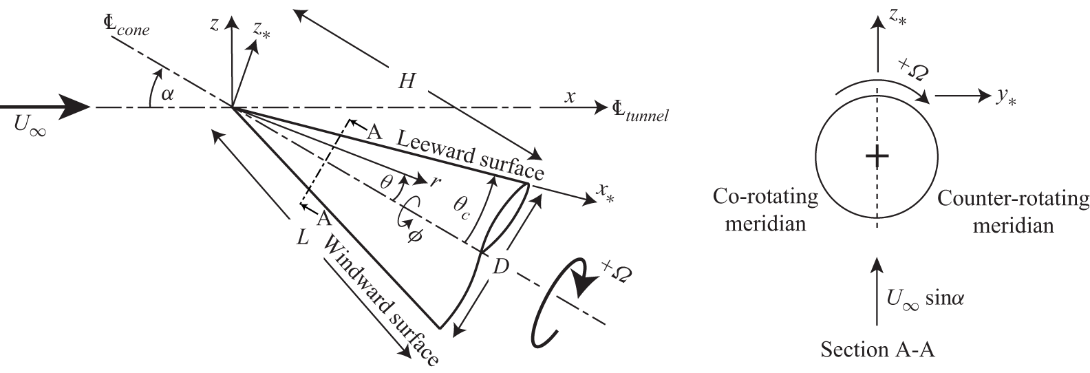


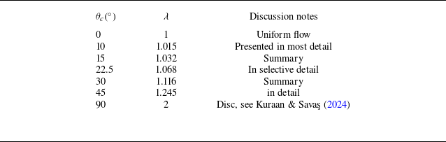


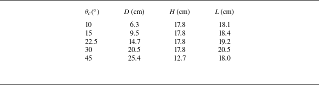


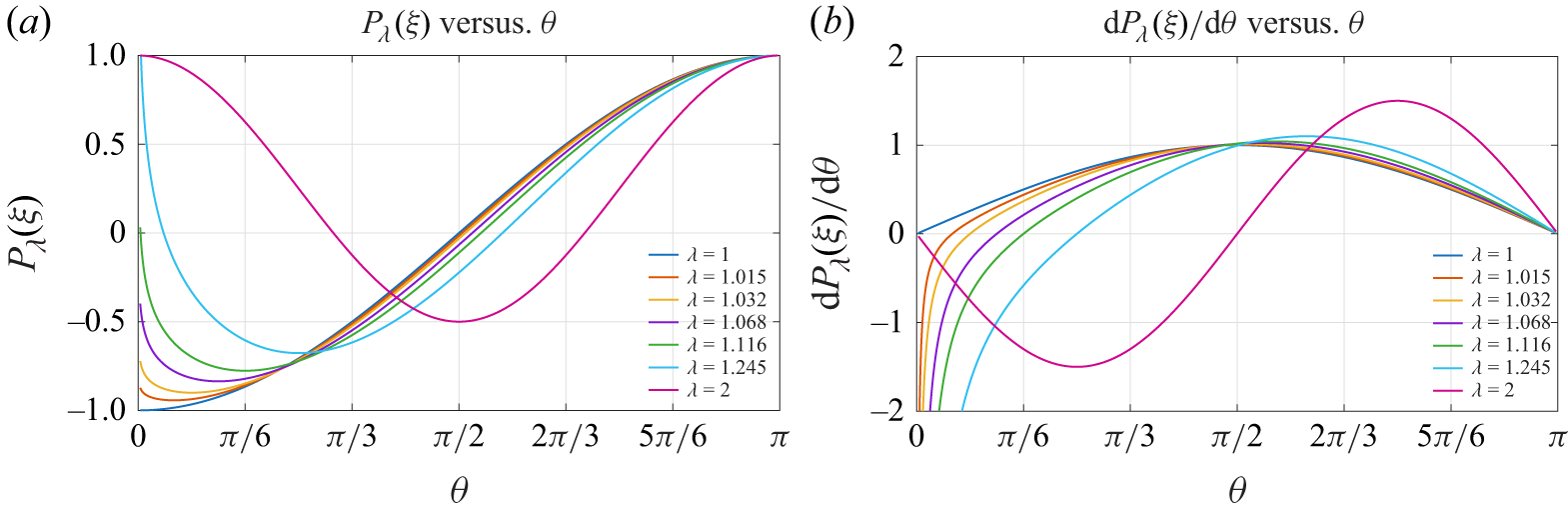


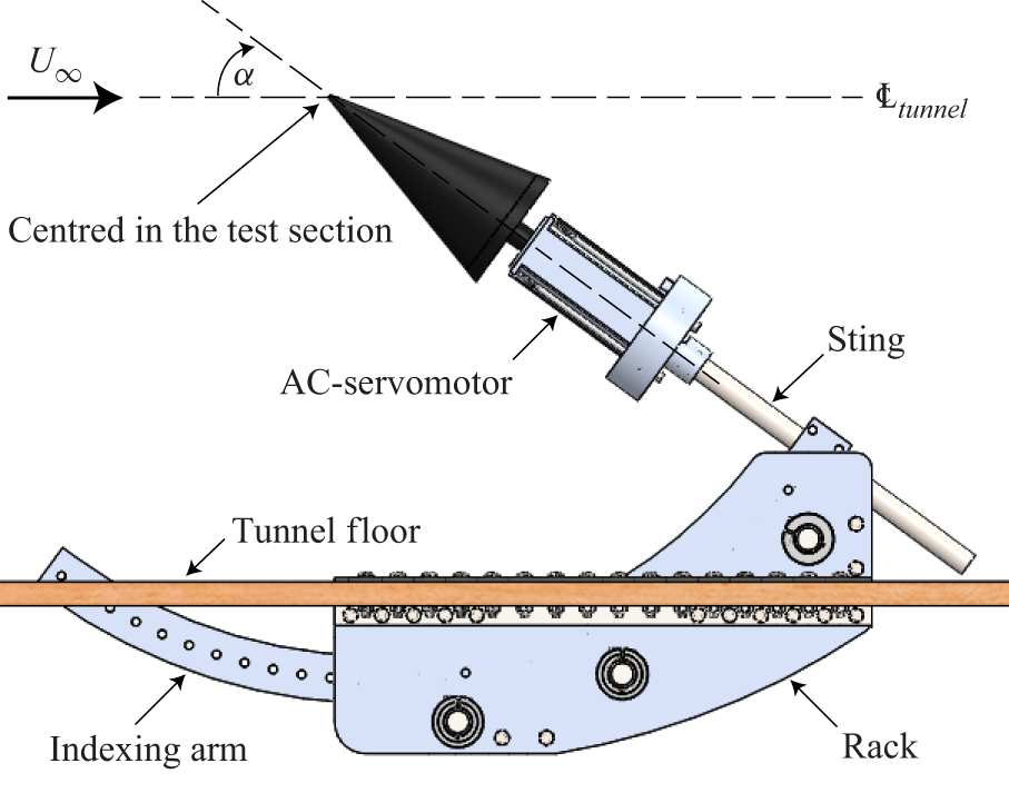

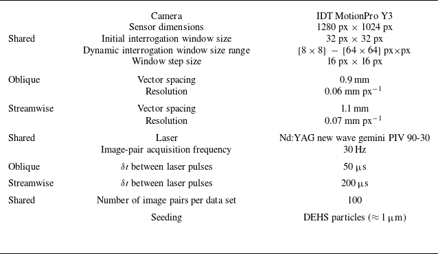
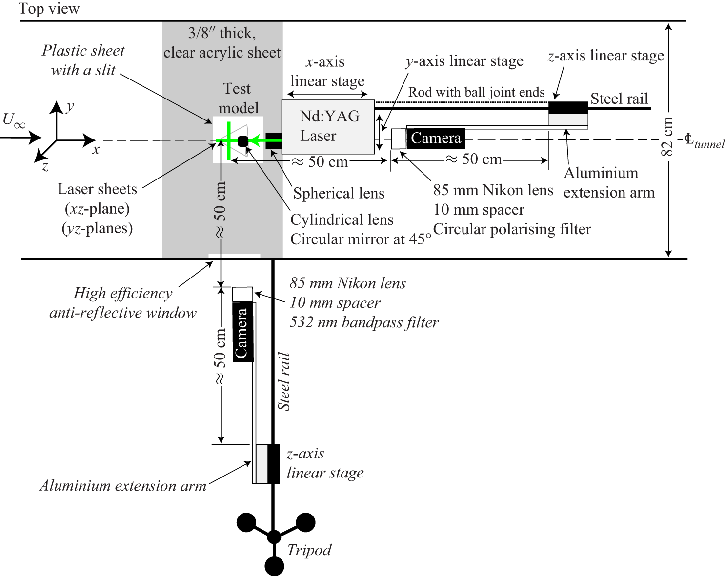
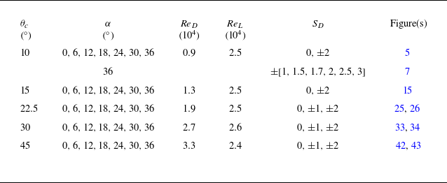
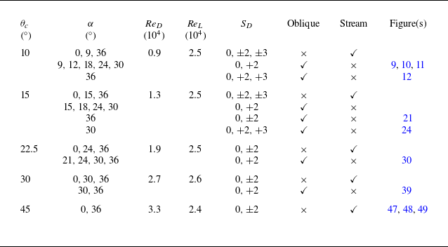
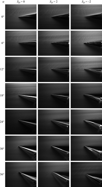


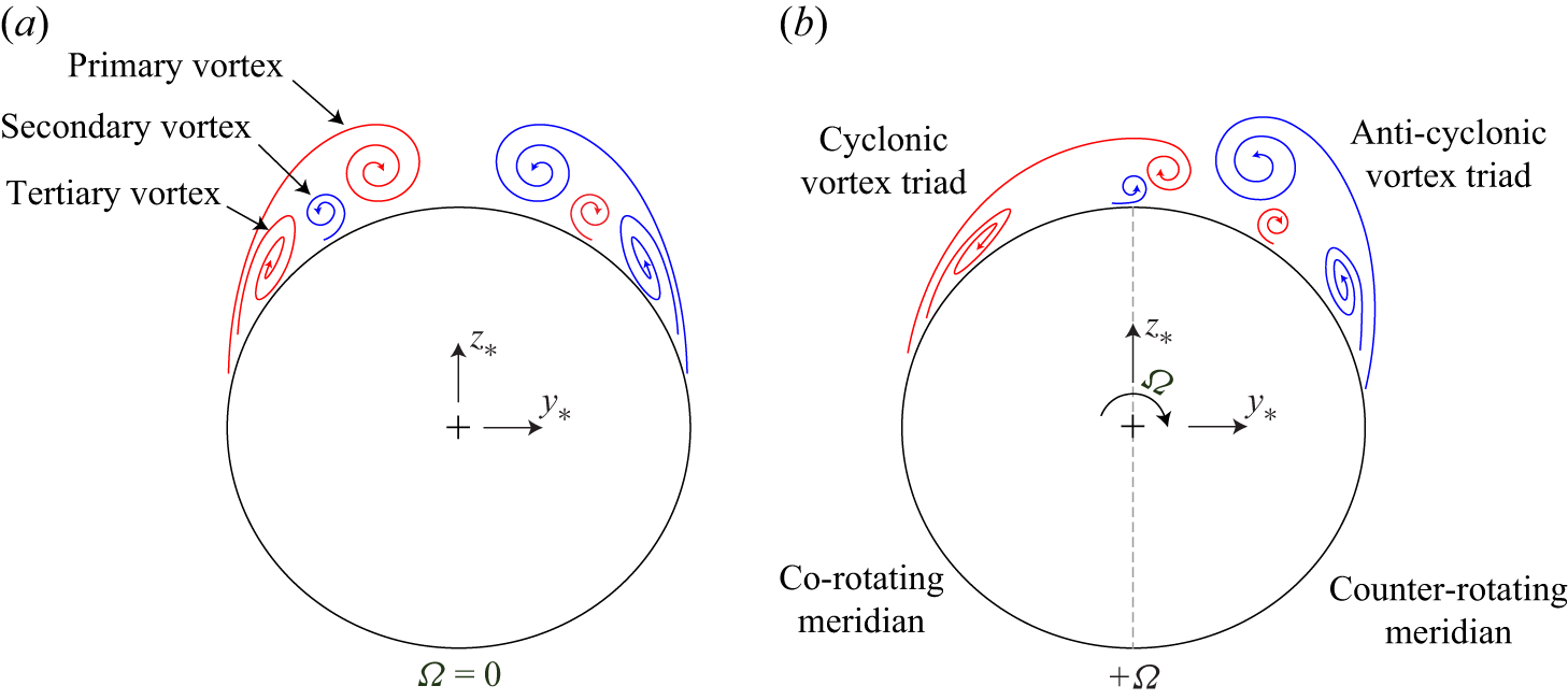


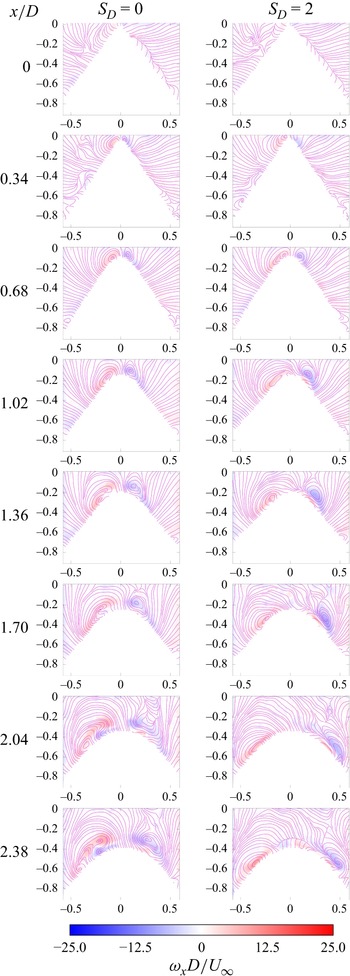


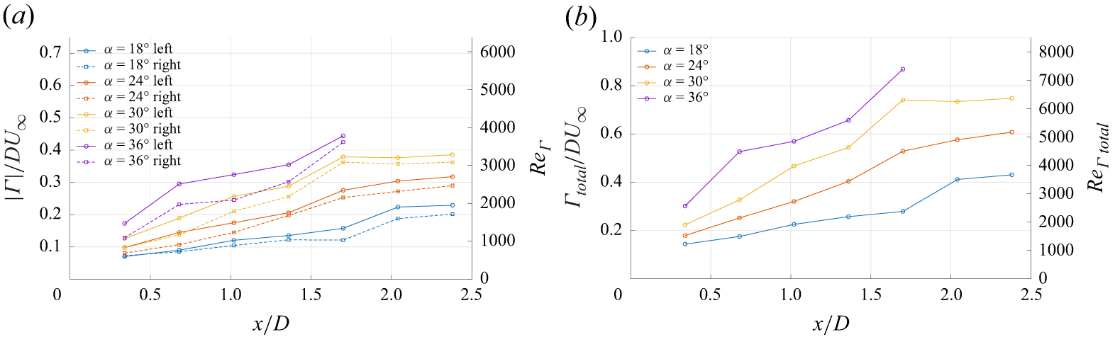


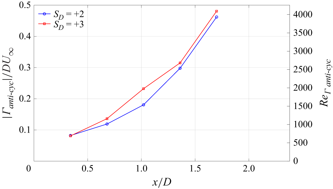


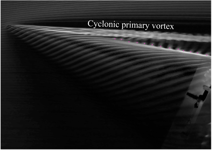


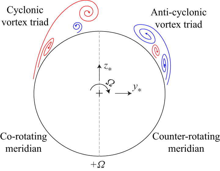


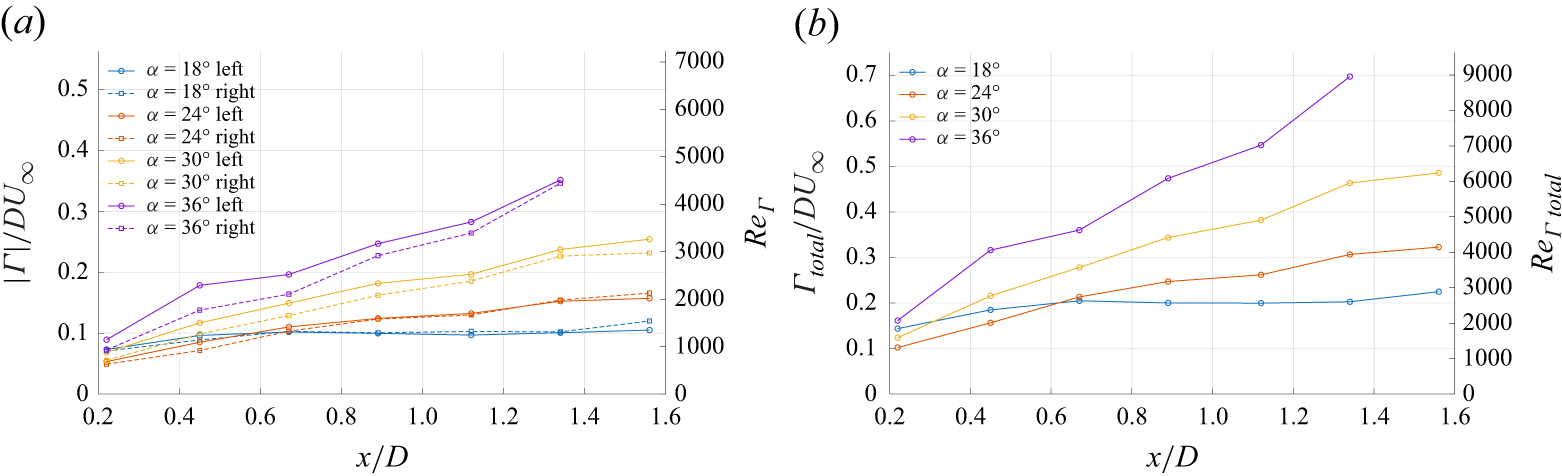


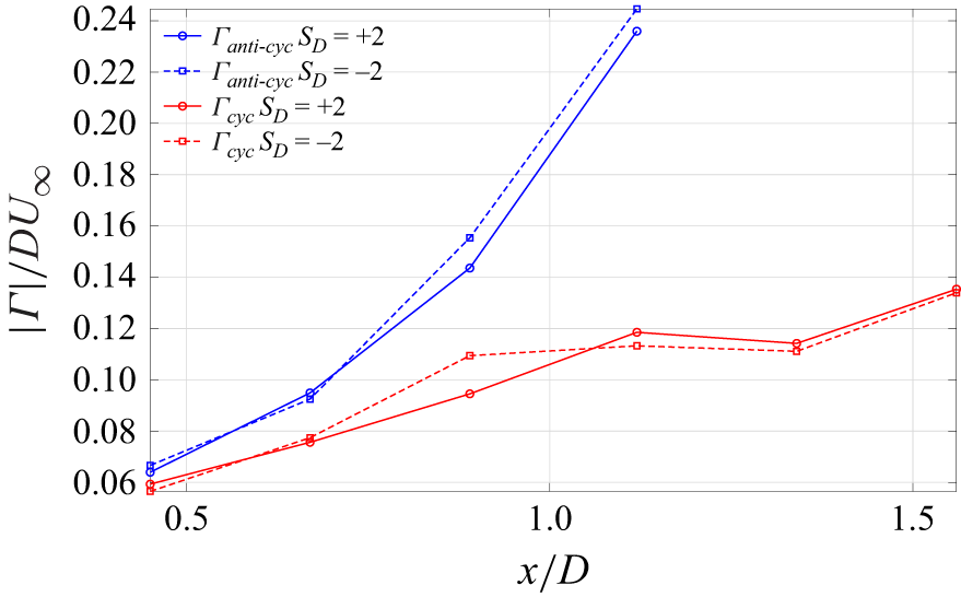


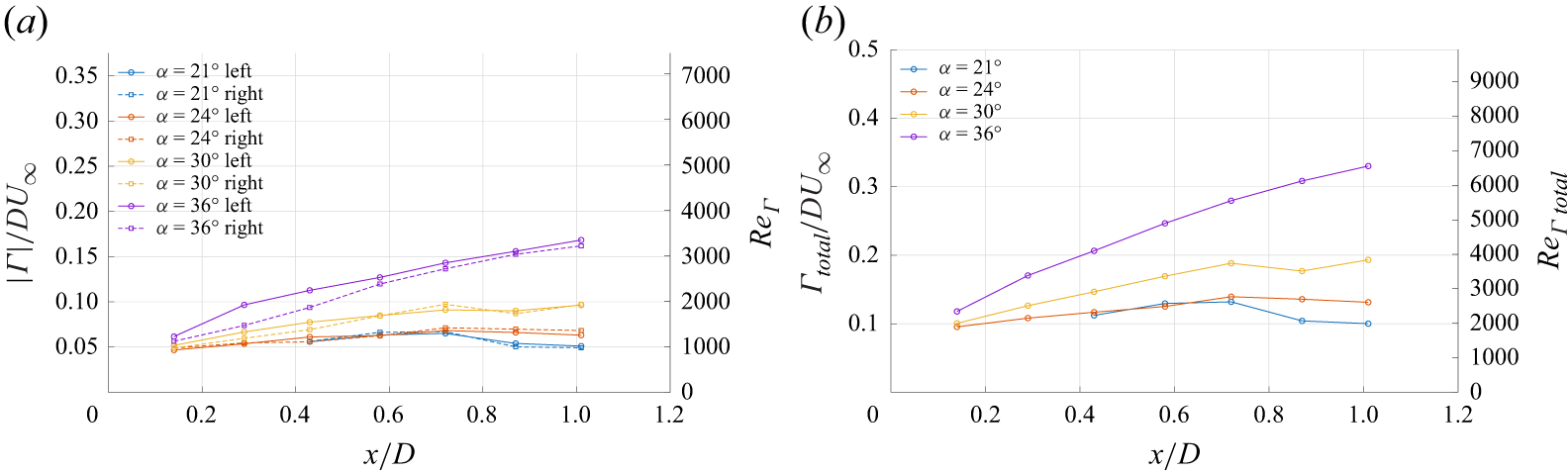


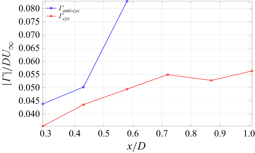


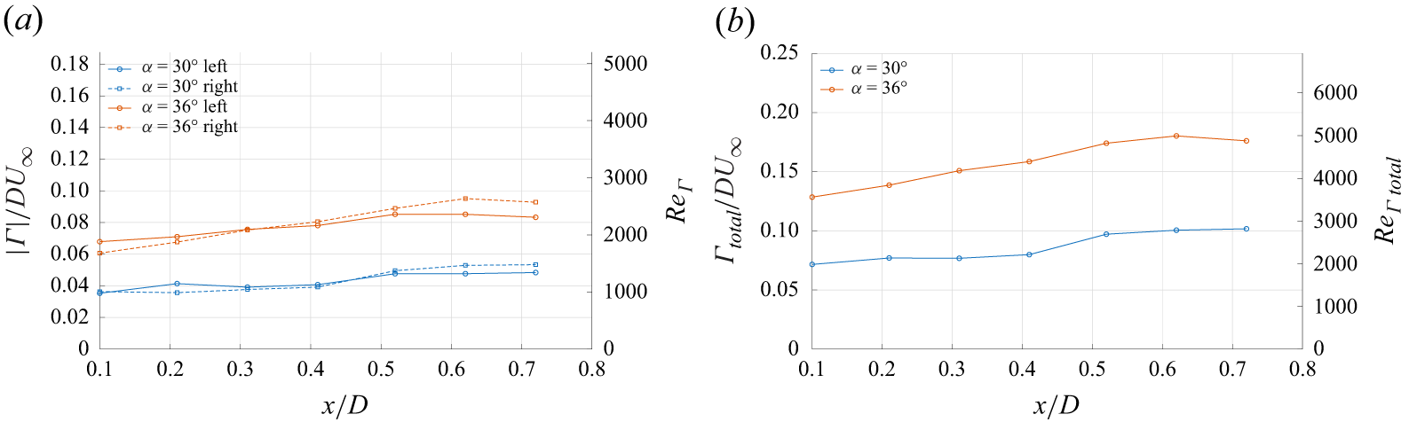


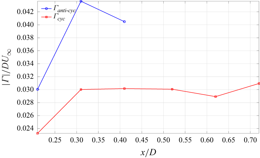


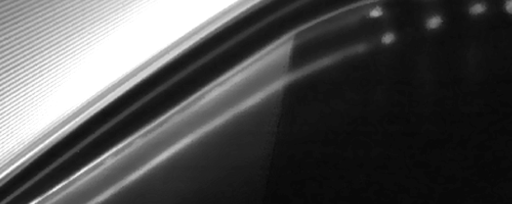


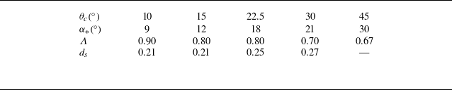


 Open access