


1. Introduction
Natural water bodies absorb and release large amounts of nutrients and greenhouse gases. The empirical parametrisations used to estimate these fluxes on a broad scale are based on relatively easily measured parameters, such as wind speed, in the case of oceans and lakes (e.g. Liss & Merlivat Reference Liss and Merlivat1986; Wanninkhof Reference Wanninkhof1992; Wanninkhof & McGillis Reference Wanninkhof and McGillis1999), and flow velocity, depth and slope, in the case of rivers and streams (e.g. Moog & Jirka Reference Moog and Jirka1999; Raymond et al. Reference Raymond, Zappa, Butman, Bott, Potter, Mulholland, Laursen, McDowell and Newbold2012; Turney & Banerjee Reference Turney and Banerjee2013). For example, based on such parametrisations for gas transfer rate, it has been estimated that lakes emit between 40 teragrams (Tg) and 200 Tg of methane per year (Sieczko et al. Reference Sieczko, Duc, Schenk, Pajala, Rudberg, Sawakuchi and Bastviken2020), rivers emit 72.8 gigagrams (Gg) of nitrogen as nitrous oxide (Marzadri et al. Reference Marzadri, Amatulli, Tonina, Bellin, Shen, Allen and Raymond2021) and 16.7–39.7 Tg of methane per year (Rocher-Ros et al. Reference Rocher-Ros, Stanley, Loken, Casson, Raymond, Liu, Amatulli and Sponseller2023), and oceans absorbed 3.0
 $\pm$
0.6 petagrams (Pg) of carbon as carbon dioxide in 2010 (Woolf et al. Reference Woolf2019). The estimated uncertainty in gas transfer velocity ranges from 5 % to 24 %, depending on the parametrisation and wind conditions, making gas transfer velocity the largest source of uncertainty in the estimated ocean–atmosphere carbon flux (Ho et al. Reference Ho, Wanninkhof, Schlosser, Ullman, Hebert and Sullivan2011; Woolf et al. Reference Woolf2019). In rivers, the scaling laws and empirical formulas that relate bulk parameters to small-scale mixing mechanisms are based on simplified, generalised channel boundary conditions, assuming lateral homogeneity, leading to greater uncertainty in conditions with macro-roughness (Ulseth et al. Reference Ulseth, Hall, Canadell, Marta, Hilary, Niayifar and Battin2019).
$\pm$
0.6 petagrams (Pg) of carbon as carbon dioxide in 2010 (Woolf et al. Reference Woolf2019). The estimated uncertainty in gas transfer velocity ranges from 5 % to 24 %, depending on the parametrisation and wind conditions, making gas transfer velocity the largest source of uncertainty in the estimated ocean–atmosphere carbon flux (Ho et al. Reference Ho, Wanninkhof, Schlosser, Ullman, Hebert and Sullivan2011; Woolf et al. Reference Woolf2019). In rivers, the scaling laws and empirical formulas that relate bulk parameters to small-scale mixing mechanisms are based on simplified, generalised channel boundary conditions, assuming lateral homogeneity, leading to greater uncertainty in conditions with macro-roughness (Ulseth et al. Reference Ulseth, Hall, Canadell, Marta, Hilary, Niayifar and Battin2019).
To produce more accurate gas transfer velocity estimates in conditions where the current simplifying assumptions do not hold, new models must be developed to relate bulk hydraulic parameters in more complex flow regimes to the order-one drivers of interfacial transfer, such as near-surface turbulent motions and coherent structures. For instance, current models do not capture the influence of counter-rotating streamwise vortices (CRSV), which are ubiquitous in rivers (Nezu, Nakagawa & Tominaga Reference Nezu, Nakagawa and Tominaga1985) and open water bodies, such as lakes and the ocean (Langmuir Reference Langmuir1938), and are associated with enhanced near-surface turbulence on multiple scales. These CRSV are considered secondary flows because they are perpendicular to and weaker than the primary streamwise flow. Langmuir cells, as one example, are CRSV driven by the wind stress interacting with waves (Langmuir Reference Langmuir1938; Craik & Leibovich Reference Craik and Leibovich1976). Takagaki et al. (Reference Takagaki, Kurose, Tsujimoto, Komori and Takahashi2015) suggested, based on their direct numerical simulations (DNS), that Langmuir cells modulate the distribution of small-scale turbulence, leading to greater interfacial scalar flux in the upwelling regions than in the downwelling regions. According to the DNS performed by Hafsi, Tejada-Martínez & Veron (Reference Hafsi, Tejada-Martínez and Veron2017), centimetre-scale Langmuir cells generated by capillary-gravity waves, with streamwise surface velocity 5–10 cm s−1, were found to increase air–sea gas transfer velocity by an order of magnitude compared to the case with only shear-driven turbulence and a flat air–water interface. Hafsi et al. (Reference Hafsi, Tejada-Martínez and Veron2017) theorised that Langmuir cells increase interfacial gas flux by promoting vertical mixing and thinning the concentration boundary layer (CBL), and their results highlight a need for temporally and spatially resolved parametrisations for gas transfer velocity. However, to our knowledge, gas transfer enhancement via Langmuir-circulation-induced surface turbulence has not been measured directly in the laboratory or field. Furthermore, the impact of similar CRSV, which form in gravity-driven open channel flows due to laterally heterogeneous boundary conditions, on gas transfer velocity has not been studied thoroughly. The interactions with the shear layer at the bed, rather than at the mixed layer to deeper water (pycnocline) interface, in the channel flow case may produce even stronger surface turbulence enhancement.
The laboratory experiments described herein and in Citerone (Reference Citerone2016) involved direct measurement of the air–water gas transfer velocity of oxygen in open channel flows with and without longitudinal bed bars intended to strengthen CRSV (see figure 1) at three bulk flow velocities. In situ and remote velocity measurements were collected during re-aeration to assess, based on turbulence metrics, lateral variation in and physical mechanisms behind said impact. In § 2, we describe the physical mechanisms and properties of the CRSV and the concepts and theory that relate turbulence to air–water gas flux rate. In § 3, we describe the experimental procedures and methods used to calculate gas transfer velocity and the flow velocity field. In § 4, we describe the impact of the bed bars on the distribution of turbulent mixing quantities, based on remote and in situ velocity measurements, and bulk gas transfer velocity.
A schematic of the secondary flows that form in open channel flow due to longitudinal bed bars, where
 $h$
is the flow depth.
$h$
is the flow depth.

2. Background
The secondary flow of interest was first described based on flow in straight, non-circular pipes and channels. In turbulent channel flow, a non-circular cross-section geometry leads iso-velocity contours (isotachs or isovels) in the cross-section to be sharply curved. Turbulent velocity fluctuations that move fluid along these contours, perpendicular to the mean flow, generate a force, proportional to the curvature of the contour, towards the corner; the kinematic boundary condition results in a pressure-gradient-driven flow along the walls away from the corner that brings anisotropic turbulence into the centre region, a process that has become known as a Prandtl secondary flow of the second kind (Prandtl Reference Prandtl1927; Nikuradse Reference Nikuradse1930; Hinze Reference Hinze1973; Nikitin, Popelenskaya & Stroh Reference Nikitin, Popelenskaya and Stroh2021). The velocity of the secondary flow depends on lateral variation in normal Reynolds stresses due to the turbulent boundary layers:
 $\overline {w} \sim \overline {u}({\partial \overline {u'v'}}/{\partial y})$
, where
$\overline {w} \sim \overline {u}({\partial \overline {u'v'}}/{\partial y})$
, where
 $u$
,
$u$
,
 $v$
and
$v$
and
 $w$
$w$
 $[\textit{LT}^{-1}]$
are velocity components in the streamwise, lateral and vertical directions, respectively (where
$[\textit{LT}^{-1}]$
are velocity components in the streamwise, lateral and vertical directions, respectively (where
 $[L]$
indicates dimensions of length, and
$[L]$
indicates dimensions of length, and
 $[T]$
indicates dimensions of time), that are separated into averaged, coherent and randomly fluctuating components through Reynolds decomposition, as follows (Reynolds & Hussain Reference Reynolds and Hussain1972; Nezu & Nakagawa Reference Nezu and Nakagawa1984):
$[T]$
indicates dimensions of time), that are separated into averaged, coherent and randomly fluctuating components through Reynolds decomposition, as follows (Reynolds & Hussain Reference Reynolds and Hussain1972; Nezu & Nakagawa Reference Nezu and Nakagawa1984):
 \begin{align} u(x,y,t) &= \overline {\langle u\rangle _{x,y}}+\tilde {u}(x,y)+u'(x,y,t), \\[-10pt] \nonumber \end{align}
 \begin{align} \tilde {u}(x,y) &= \overline {u(x,y,t)-\langle u\rangle _{x,y}(t)}=\overline {u}(x,y)-\overline {\langle u\rangle _{x,y}}, \\[-10pt] \nonumber \end{align}
 \begin{align} u'(x,y,t) &= u(x,y,t)-\overline {u}(x,y), \\[9pt] \nonumber \end{align}
where
 $\overline {X}$
denotes temporal averaging of
$\overline {X}$
denotes temporal averaging of
 $X$
, and
$X$
, and
 $\langle X\rangle _{x/y}$
denotes spatial averaging of
$\langle X\rangle _{x/y}$
denotes spatial averaging of
 $X$
in the
$X$
in the
 $x$
or
$x$
or
 $y$
directions, respectively. Note that this description applies to
$y$
directions, respectively. Note that this description applies to
 $v$
and
$v$
and
 $w$
as well, and temporal averaging could be exchanged with averaging in a homogeneous direction, such as
$w$
as well, and temporal averaging could be exchanged with averaging in a homogeneous direction, such as
 $x$
, for use in spatial turbulence spectra calculations (e.g.
$x$
, for use in spatial turbulence spectra calculations (e.g.
 $u'=u-\langle u\rangle _x$
). We associate relative secondary flow strength with the value of
$u'=u-\langle u\rangle _x$
). We associate relative secondary flow strength with the value of
 $\max( |\langle \tilde {u_s}\rangle _x|)/\langle \overline {u_s}\rangle _{x,y}$
, where
$\max( |\langle \tilde {u_s}\rangle _x|)/\langle \overline {u_s}\rangle _{x,y}$
, where
 $u_s$
is the surface streamwise velocity (Soldati, Orlandi & Pirozzoli Reference Soldati, Orlandi and Pirozzoli2025).
$u_s$
is the surface streamwise velocity (Soldati, Orlandi & Pirozzoli Reference Soldati, Orlandi and Pirozzoli2025).
Prandtl secondary flows of the second kind also arise more generally in turbulent boundary layer flow over surfaces (e.g. Anderson et al. Reference Anderson, Barros, Christensen and Awasthi2015; Vanderwel & Ganapathisubramani Reference Vanderwel and Ganapathisubramani2015; Medjnoun, Vanderwel & Ganapathisubramani Reference Medjnoun, Vanderwel and Ganapathisubramani2018; Wangsawijaya et al. Reference Wangsawijaya, Baidya, Chung, Marusic and Hutchins2020), ducts (e.g. Goldstein & Tuan Reference Goldstein and Tuan1998) and wide open channels (e.g. Culbertson Reference Culbertson1967; Kinoshita Reference Kinoshita1967; Karez Reference Karez1973; Nezu & Nakagawa Reference Nezu and Nakagawa1984) with spanwise heterogeneity. In wide channels, the diameter of these secondary flows is equal to the channel depth (Culbertson Reference Culbertson1967; Kinoshita Reference Kinoshita1967; Karez Reference Karez1973). It follows that the most effective spacing of longitudinal bed elements to support these cells is twice the cells’ diameter. In previous work, it was found that placing longitudinal bars (e.g. Nezu & Nakagawa Reference Nezu and Nakagawa1984; Wang & Cheng Reference Wang and Cheng2006) or roughness strips (e.g. Wang & Cheng Reference Wang and Cheng2006; Willingham et al. Reference Willingham, Anderson, Christensen and Barros2014; Stoesser, McSherry & Fraga Reference Stoesser, McSherry and Fraga2015) along the bed, with lateral spacing of twice the flow depth in channel flow, or 90 % of the boundary layer thickness in a turbulent boundary layer (Vanderwel & Ganapathisubramani Reference Vanderwel and Ganapathisubramani2015), stabilises and enhances CRSV, due to the steeper cross-stream isotach curvature imposed by the bed features. These secondary flows can also be thought of as redistributing momentum due to local imbalances between turbulent kinetic energy (TKE) production and dissipation, with maximal Reynolds stress, excess TKE production, and downwelling in the ‘high momentum pathways’ between bars or over roughness strips (e.g. Anderson et al. Reference Anderson, Barros, Christensen and Awasthi2015; Vanderwel & Ganapathisubramani Reference Vanderwel and Ganapathisubramani2015). Further, macro-roughness, such as submerged vegetation canopies, in open channel flow is associated with a ‘spectral shortcut’ phenomenon whereby turbulent structures are generated at multiple scales, interacting with each other, and fine-scale shear boundary layers form, leading to greater total dissipation rates (Finnigan Reference Finnigan2000; Nepf & Vivoni Reference Nepf and Vivoni2000; Nezu & Sanjou Reference Nezu and Sanjou2008; King, Tinoco & Cowen Reference King, Tinoco and Cowen2012). This process is exhibited in the TKE spectral distribution as dual inertial subranges (Zhao et al. Reference Zhao, Tang, Yan, Liang and Zheng2020). Katul et al. (Reference Katul, Manes, Porporato, Bou-Zeid and Chamecki2015) also described a similar phenomenon that they refer to as an energy ‘bottleneck’ observed at wavenumber values near
 $0.1/\eta$
. Johnson & Cowen (Reference Johnson and Cowen2017) also observed something like a dual inertial subrange, as well as anisotropy at large and small turbulence length scales, in the spectral signature on the surface above laterally heterogeneous bed roughness. The multi-scale, near-surface turbulent motions associated with these currents impact mixing and interfacial gas transport.
$0.1/\eta$
. Johnson & Cowen (Reference Johnson and Cowen2017) also observed something like a dual inertial subrange, as well as anisotropy at large and small turbulence length scales, in the spectral signature on the surface above laterally heterogeneous bed roughness. The multi-scale, near-surface turbulent motions associated with these currents impact mixing and interfacial gas transport.
Air–water interfacial transport of weakly soluble gases, such as oxygen, carbon dioxide, methane and nitrous oxide, is limited by molecular diffusive flux rate through the aqueous-side, molecular diffusive sublayer (DSL), also known as the Batchelor sublayer, where turbulent mixing is inhibited by viscosity, and flux depends on the molecular diffusivity
 $D_m\ [L^2T^{-1}]$
of the dissolved gas and the concentration gradient as described by Fick’s law (Fick Reference Fick1855; Nernst Reference Nernst1904; Lewis & Whitman Reference Lewis and Whitman1924; Liss Reference Liss1973; Cussler Reference Cussler1984; Variano & Cowen Reference Variano and Cowen2013). The concentration gradient in the DSL relates inversely to the DSL’s thickness
$D_m\ [L^2T^{-1}]$
of the dissolved gas and the concentration gradient as described by Fick’s law (Fick Reference Fick1855; Nernst Reference Nernst1904; Lewis & Whitman Reference Lewis and Whitman1924; Liss Reference Liss1973; Cussler Reference Cussler1984; Variano & Cowen Reference Variano and Cowen2013). The concentration gradient in the DSL relates inversely to the DSL’s thickness
 $\delta _d$
, which is related to that of the viscous sublayer,
$\delta _d$
, which is related to that of the viscous sublayer,
 $\delta _v$
, by the Schmidt number
$\delta _v$
, by the Schmidt number
 $ \textit{Sc} $
(i.e.
$ \textit{Sc} $
(i.e.
 $\delta _c=\delta _vSc^{-n}$
, where
$\delta _c=\delta _vSc^{-n}$
, where
 $Sc=\nu /D_m$
, and
$Sc=\nu /D_m$
, and
 $\nu$
is the kinematic viscosity of the liquid
$\nu$
is the kinematic viscosity of the liquid
 $[L^2T^{-1}]$
) and is generally less than 1–2 mm thick (e.g. McKenna & McGillis Reference McKenna and McGillis2004). The concentration difference across the DSL depends on turbulent stirring in the rest of the CBL, which is typically 0.5 mm to 1 cm thick in these contexts (e.g. Shankaran & Hearst Reference Shankaran and Hearst2025). The interfacial mass flux
$[L^2T^{-1}]$
) and is generally less than 1–2 mm thick (e.g. McKenna & McGillis Reference McKenna and McGillis2004). The concentration difference across the DSL depends on turbulent stirring in the rest of the CBL, which is typically 0.5 mm to 1 cm thick in these contexts (e.g. Shankaran & Hearst Reference Shankaran and Hearst2025). The interfacial mass flux
 $F\ [\textit{ML}^{-2}T^{-1}]$
(where
$F\ [\textit{ML}^{-2}T^{-1}]$
(where
 $[M]$
indicates units of mass) is described as a function of the difference between equilibrated liquid concentration
$[M]$
indicates units of mass) is described as a function of the difference between equilibrated liquid concentration
 $C_s\ [\textit{ML}^{-3}]$
and the concentration of gas in the bulk liquid,
$C_s\ [\textit{ML}^{-3}]$
and the concentration of gas in the bulk liquid,
 $C_b\ [ \textit{ML}^{-3}]$
, and a gas transfer velocity parameter
$C_b\ [ \textit{ML}^{-3}]$
, and a gas transfer velocity parameter
 $K\ [\textit{LT}^{-1}]$
that captures the physical properties of the CBL:
$K\ [\textit{LT}^{-1}]$
that captures the physical properties of the CBL:
 \begin{align} F = K\,\Delta C=K(C_s-C_b). \end{align}
Near-surface turbulent motions impact
 $K$
by generating steep concentration gradients near the water surface as they bring fluid with concentrations similar to
$K$
by generating steep concentration gradients near the water surface as they bring fluid with concentrations similar to
 $C_b$
towards the air–water interface, where the concentration is
$C_b$
towards the air–water interface, where the concentration is
 $C_s$
. These motions are referred to as renewal events, and their characteristic duration is referred to as the renewal time scale
$C_s$
. These motions are referred to as renewal events, and their characteristic duration is referred to as the renewal time scale
 $\tau \ [T]$
, representing the average time a parcel of water from below the DSL is in contact with the DSL. The surface renewal model relates
$\tau \ [T]$
, representing the average time a parcel of water from below the DSL is in contact with the DSL. The surface renewal model relates
 $K$
to
$K$
to
 $\tau$
through scaling principles (Higbie Reference Higbie1935; Danckwerts Reference Danckwerts1951):
$\tau$
through scaling principles (Higbie Reference Higbie1935; Danckwerts Reference Danckwerts1951):
 \begin{align} K \sim \sqrt {\frac {D_m}{\tau }}. \end{align}
When considering which time scale best represents this average renewal time, one can consider the following three metrics: the shortest time scale of concentration fluctuations, the Batchelor scale (
 $\tau _{\textit{SC}}$
 $[T]$
; Batchelor Reference Batchelor1959); the time scale of large energy-containing eddies or ‘outer scale’ of turbulence (
$[T]$
; Batchelor Reference Batchelor1959); the time scale of large energy-containing eddies or ‘outer scale’ of turbulence (
 $\tau _{\textit{LE}}$
 $[T]$
); and the time scale of small momentum-dissipating eddies, the Kolmogorov scale or the ‘inner scale’ of turbulence (
$[T]$
); and the time scale of small momentum-dissipating eddies, the Kolmogorov scale or the ‘inner scale’ of turbulence (
 $\tau _{\textit{SE}}$
, also known as
$\tau _{\textit{SE}}$
, also known as
 $\eta _{\tau }$
 $[T]$
; Kolmogorov et al. Reference Kolmogorov1941). These scales are defined as
$[T]$
; Kolmogorov et al. Reference Kolmogorov1941). These scales are defined as
 \begin{align} \tau _{\textit{SC}} &= \sqrt {\frac {D_m}{\varepsilon }}, \\[-10pt] \nonumber \end{align}
 \begin{align} \tau _{\textit{LE}} &= \frac {L_{33}}{\sqrt {\overline {w'^2}}} , \\[-10pt] \nonumber \end{align}
 \begin{align} \tau _{\textit{SE}} &= \sqrt {\frac {\nu }{\varepsilon }}, \\[9pt] \nonumber \end{align}
where
 $\varepsilon$
is the TKE dissipation rate
$\varepsilon$
is the TKE dissipation rate
 $[L^2T^{-3}]$
,
$[L^2T^{-3}]$
,
 $L_{33}$
is the characteristic length scale of large eddies (i.e. the vertical turbulence integral length scale)
$L_{33}$
is the characteristic length scale of large eddies (i.e. the vertical turbulence integral length scale)
 $[L]$
, and
$[L]$
, and
 $\sqrt {\overline {w^{\prime 2}}}$
is the characteristic velocity scale of large eddies (i.e. the temporal root mean square of the vertical velocity fluctuation
$\sqrt {\overline {w^{\prime 2}}}$
is the characteristic velocity scale of large eddies (i.e. the temporal root mean square of the vertical velocity fluctuation
 $w^{\prime}$
)
$w^{\prime}$
)
 $[\textit{LT}^{-1}]$
. Note that by scaling principles,
$[\textit{LT}^{-1}]$
. Note that by scaling principles,
 $\varepsilon \sim \overline {w^{\prime 2}}/\tau _{\textit{LE}}$
. The ratios of the above time scales are the Schmidt number to the power
$\varepsilon \sim \overline {w^{\prime 2}}/\tau _{\textit{LE}}$
. The ratios of the above time scales are the Schmidt number to the power
 $-1/2$
(2.9); the turbulent Reynolds number (
$-1/2$
(2.9); the turbulent Reynolds number (
 $ \textit{Re}_{t,1},\ Re_{t,2},\ Re_{t,3}$
, describing turbulence in the streamwise, transverse and vertical directions, respectively) to the power
$ \textit{Re}_{t,1},\ Re_{t,2},\ Re_{t,3}$
, describing turbulence in the streamwise, transverse and vertical directions, respectively) to the power
 $1/2$
(2.10); and the ratio of the two (2.11):
$1/2$
(2.10); and the ratio of the two (2.11):
 \begin{align} Sc^{-1/2} &= \tau _{\textit{SC}}/\tau _{\textit{SE}}=\sqrt {D_m/\nu }, \\[-10pt] \nonumber \end{align}
 \begin{align} Re_{t,3}^{1/2} &= \tau _{\textit{LE}}/\tau _{\textit{SE}} = \left (L_{33}\sqrt {\overline {w'^2}}/\nu \right )^{1/2} \!, \\[-10pt] \nonumber \end{align}
 \begin{align} (Sc\,Re_{t,3})^{-1/2} &= \tau _{\textit{SC}}/\tau _{\textit{LE}} = \left (D_m\Big/\left [L_{33}\sqrt {\overline {w'^2}}\right ]\right )^{1/2} \!. \\[9pt] \nonumber \end{align}
The ratios given by (2.9)–(2.11) indicate which time scales have a dominant effect on gas transfer velocity (Theofanous, Houze & Brumfield Reference Theofanous, Houze and Brumfield1976; Herlina & Jirka Reference Herlina and Jirka2008). For example, if
 $ \textit{Sc} $
and
$ \textit{Sc} $
and
 $ \textit{Re}_{t,3}$
are large, then velocity fluctuations are much slower than possible concentration fluctuations, and large eddies are much slower than small eddies. Thus small eddies would contribute more turbulent mass flux,
$ \textit{Re}_{t,3}$
are large, then velocity fluctuations are much slower than possible concentration fluctuations, and large eddies are much slower than small eddies. Thus small eddies would contribute more turbulent mass flux,
 $c'w'$
, and perform the most mixing of the gas, while the large eddies would more likely stir patches of dissolved gas. Furthermore,
$c'w'$
, and perform the most mixing of the gas, while the large eddies would more likely stir patches of dissolved gas. Furthermore,
 $ \textit{Re}_t$
controls the energy flux behaviour of free-surface turbulence, where at low
$ \textit{Re}_t$
controls the energy flux behaviour of free-surface turbulence, where at low
 $ \textit{Re}_t$
, energy transfers from large to small scales at all scales, but at high
$ \textit{Re}_t$
, energy transfers from large to small scales at all scales, but at high
 $ \textit{Re}_t$
, energy can partially transfer from smaller to larger scales in an inverse cascade (Lovecchio, Zonta & Soldati Reference Lovecchio, Zonta and Soldati2015). Therefore, parametrisations relating gas transfer velocity to turbulence metrics are typically based on either the large eddy model (LEM) (Fortescue & Pearson Reference Fortescue and Pearson1967), which sets the renewal time scale
$ \textit{Re}_t$
, energy can partially transfer from smaller to larger scales in an inverse cascade (Lovecchio, Zonta & Soldati Reference Lovecchio, Zonta and Soldati2015). Therefore, parametrisations relating gas transfer velocity to turbulence metrics are typically based on either the large eddy model (LEM) (Fortescue & Pearson Reference Fortescue and Pearson1967), which sets the renewal time scale
 $\tau$
equal to the large eddy time scale
$\tau$
equal to the large eddy time scale
 $\tau _{\textit{LE}}$
, or the small eddy model (SEM), which uses the Kolmogorov time scale
$\tau _{\textit{LE}}$
, or the small eddy model (SEM), which uses the Kolmogorov time scale
 $\tau _{\textit{SE}}$
to represent the renewal time scale (Banerjee, Scott & Rhodes Reference Banerjee, Scott and Rhodes1968; Lamont & Scott Reference Lamont and Scott1970; Turney & Banerjee Reference Turney and Banerjee2013), as in the equations
$\tau _{\textit{SE}}$
to represent the renewal time scale (Banerjee, Scott & Rhodes Reference Banerjee, Scott and Rhodes1968; Lamont & Scott Reference Lamont and Scott1970; Turney & Banerjee Reference Turney and Banerjee2013), as in the equations
 \begin{align} (\text{LEM})\quad K &\sim \sqrt {\frac {D_m}{\tau _{\textit{LE}}}} = \sqrt {\frac {D_m\sqrt {\overline {w'^2}}}{L_{33}}} = Sc^{-1/2}\,Re_{t,3}^{-1/2}\sqrt {\overline {w'^2}}\rightarrow \frac {KSc^{1/2}}{\sqrt {\overline {w'^2}}}\propto Re_{t,3}^{-1/2}, \\[-10pt] \nonumber \end{align}
 \begin{align} \nonumber (\text{SEM})\quad K &\sim \sqrt {\frac {D_m}{\tau _{\textit{SE}}}} = \sqrt {D_m}\left (\frac {\varepsilon }{\nu }\right )^{1/4} = Sc^{-1/2}(\varepsilon \nu )^{1/4} \rightarrow \frac {KSc^{1/2}}{\sqrt {\overline {w'^2}}}\propto Re_{t,3}^{-1/4}\\& \rightarrow \hat {K}_{\textit{SEM}} = C_{\textit{SE}} Sc^{-n}(\varepsilon\nu )^{1/4}, \\[9pt] \nonumber \end{align}
where
 $\hat {X}$
indicates the modelled or estimated value of
$\hat {X}$
indicates the modelled or estimated value of
 $X$
,
$X$
,
 $C_{\textit{SE}}$
is an empirical constant, and
$C_{\textit{SE}}$
is an empirical constant, and
 $n=1/2$
for the interfaces of interest, which are rough and mobile, as opposed to flat surfaces where
$n=1/2$
for the interfaces of interest, which are rough and mobile, as opposed to flat surfaces where
 $n=2/3$
(Lamont & Scott Reference Lamont and Scott1970; Holmén & Liss Reference Holmén and Liss1984; Jähne et al. Reference Jähne, Fischer, Ilmberger, Libner, Weiss, Imboden, Lemnin and Jaquet1984; Coantic Reference Coantic1986; Calderbank & Moo-Young Reference Calderbank and Moo-Young1995). Theofanous et al. (Reference Theofanous, Houze and Brumfield1976) and Herlina & Wissink (Reference Herlina and Wissink2019) suggest that the LEM should be applied at low turbulent Reynolds numbers (i.e.
$n=2/3$
(Lamont & Scott Reference Lamont and Scott1970; Holmén & Liss Reference Holmén and Liss1984; Jähne et al. Reference Jähne, Fischer, Ilmberger, Libner, Weiss, Imboden, Lemnin and Jaquet1984; Coantic Reference Coantic1986; Calderbank & Moo-Young Reference Calderbank and Moo-Young1995). Theofanous et al. (Reference Theofanous, Houze and Brumfield1976) and Herlina & Wissink (Reference Herlina and Wissink2019) suggest that the LEM should be applied at low turbulent Reynolds numbers (i.e.
 $ \textit{Re}_{t,1}\ \lt \ 500$
), when there is less separation between large eddy and small eddy time scales, and that the SEM is valid for cases with higher turbulent Reynolds numbers (i.e.
$ \textit{Re}_{t,1}\ \lt \ 500$
), when there is less separation between large eddy and small eddy time scales, and that the SEM is valid for cases with higher turbulent Reynolds numbers (i.e.
 $ \textit{Re}_{t,1}\ \gt \ 500$
), in which there is greater separation between large and small eddy time scales. This
$ \textit{Re}_{t,1}\ \gt \ 500$
), in which there is greater separation between large and small eddy time scales. This
 $ \textit{Re}_t$
threshold approach is reasonably consistent with other previous studies, such as Chu & Jirka (Reference Chu and Jirka1992). The SEM is expected to be more accurate in the experiments described herein, which represent natural and industrial flows of interest.
$ \textit{Re}_t$
threshold approach is reasonably consistent with other previous studies, such as Chu & Jirka (Reference Chu and Jirka1992). The SEM is expected to be more accurate in the experiments described herein, which represent natural and industrial flows of interest.
Note that
 $Sc^{-1/2}$
, the ratio between the Batchelor time scale and the Kolmogorov time scale, arises in both (2.12) and (2.13). Therefore,
$Sc^{-1/2}$
, the ratio between the Batchelor time scale and the Kolmogorov time scale, arises in both (2.12) and (2.13). Therefore,
 $K$
can be compared across different liquids, temperatures and gases based on their relative Schmidt numbers, using the relation
$K$
can be compared across different liquids, temperatures and gases based on their relative Schmidt numbers, using the relation
 \begin{align} K _2 = K _1\left (\frac {Sc_2}{Sc_1}\right )^{-1/2} \!. \end{align}
The empirical constant
 $C_{\textit{SE}}$
in (2.13) is inconsistent across observational data. Values range from 0.17 to 0.62 (Tokoro et al. Reference Tokoro, Kayanne, Watanabe, Nadaoka, Tamura, Nozaki, Kato and Negishi2008; Vachon, Prairie & Cole Reference Vachon, Prairie and Cole2010). Katul et al. (Reference Katul, Mammarella, Grönholm and Vesala2018) analytically derived a constant
$C_{\textit{SE}}$
in (2.13) is inconsistent across observational data. Values range from 0.17 to 0.62 (Tokoro et al. Reference Tokoro, Kayanne, Watanabe, Nadaoka, Tamura, Nozaki, Kato and Negishi2008; Vachon, Prairie & Cole Reference Vachon, Prairie and Cole2010). Katul et al. (Reference Katul, Mammarella, Grönholm and Vesala2018) analytically derived a constant
 $C_{\textit{SE}}=\sqrt {2/15}=0.36$
by scaling
$C_{\textit{SE}}=\sqrt {2/15}=0.36$
by scaling
 $\varepsilon$
with the second-order structure function of the velocity using the von Kármán–Howarth equation, the Dawson function, and K41 theory (Kolmogorov Reference Kolmogorov1941; Katul et al. Reference Katul, Manes, Porporato, Bou-Zeid and Chamecki2015). Others have found empirically that
$\varepsilon$
with the second-order structure function of the velocity using the von Kármán–Howarth equation, the Dawson function, and K41 theory (Kolmogorov Reference Kolmogorov1941; Katul et al. Reference Katul, Manes, Porporato, Bou-Zeid and Chamecki2015). Others have found empirically that
 $C_{\textit{SE}}$
is consistently in the range 0.40–0.42 (e.g. Lamont & Scott Reference Lamont and Scott1970; Zappa et al. Reference Zappa, McGillis, Raymond, Edson, Hintsa, Zemmelink, Dacey and Ho2007). Still others suggest that
$C_{\textit{SE}}$
is consistently in the range 0.40–0.42 (e.g. Lamont & Scott Reference Lamont and Scott1970; Zappa et al. Reference Zappa, McGillis, Raymond, Edson, Hintsa, Zemmelink, Dacey and Ho2007). Still others suggest that
 $C_{\textit{SE}}$
is a function of the TKE dissipation rate, such as
$C_{\textit{SE}}$
is a function of the TKE dissipation rate, such as
 $C_{\textit{SE}}=0.17\log\varepsilon + 1.11$
for cases with
$C_{\textit{SE}}=0.17\log\varepsilon + 1.11$
for cases with
 $\varepsilon \lt 10^6\,\rm m^2\,s^{-3}$
and surfactants present (Wang et al. Reference Wang, Liao, Fillingham and Bootsma2015).
$\varepsilon \lt 10^6\,\rm m^2\,s^{-3}$
and surfactants present (Wang et al. Reference Wang, Liao, Fillingham and Bootsma2015).
Along with the SEM, we consider the surface divergence model (SDM) to quantify the impact of CRSV on gas transfer velocity because the mean square surface velocity divergence
 $\overline {\beta^{\prime 2}}\ [T^{-2}]$
is proportional to the normal TKE dissipation rate divided by kinematic viscosity; thus
$\overline {\beta^{\prime 2}}\ [T^{-2}]$
is proportional to the normal TKE dissipation rate divided by kinematic viscosity; thus
 $\sqrt {\overline {\beta^{\prime 2}}}$
represents the reciprocal of the time scale (
$\sqrt {\overline {\beta^{\prime 2}}}$
represents the reciprocal of the time scale (
 $1/\tau _{\textit{SE}}$
) of turbulent motions that are near and normal to the air–water interface (e.g. Teixeira & Belcher Reference Teixeira and Belcher2000). The SDM represents the renewal time scale in (2.5) as the reciprocal of
$1/\tau _{\textit{SE}}$
) of turbulent motions that are near and normal to the air–water interface (e.g. Teixeira & Belcher Reference Teixeira and Belcher2000). The SDM represents the renewal time scale in (2.5) as the reciprocal of
 $\sqrt {\overline {\beta^{\prime 2}}}$
takes the form (Chan & Scriven Reference Chan and Scriven1970; McCready, Vassiliadou & Hanratty Reference McCready, Vassiliadou and Hanratty1986)
$\sqrt {\overline {\beta^{\prime 2}}}$
takes the form (Chan & Scriven Reference Chan and Scriven1970; McCready, Vassiliadou & Hanratty Reference McCready, Vassiliadou and Hanratty1986)
 \begin{align} K &=c\sqrt {D_m\sqrt {\overline {\beta '^2}}}, \end{align}
where
 $c$
is an empirical coefficient that varies (0.2–0.71) across studies (McCready et al. Reference McCready, Vassiliadou and Hanratty1986; Xu, Khoo & Carpenter Reference Xu, Khoo and Carpenter2006; Turney & Banerjee Reference Turney and Banerjee2013). Hafsi et al. (Reference Hafsi, Tejada-Martínez and Veron2017) found both the SEM (
$c$
is an empirical coefficient that varies (0.2–0.71) across studies (McCready et al. Reference McCready, Vassiliadou and Hanratty1986; Xu, Khoo & Carpenter Reference Xu, Khoo and Carpenter2006; Turney & Banerjee Reference Turney and Banerjee2013). Hafsi et al. (Reference Hafsi, Tejada-Martínez and Veron2017) found both the SEM (
 $C_{\textit{SE}}=0.419$
) and SDM (
$C_{\textit{SE}}=0.419$
) and SDM (
 $c = 0.71$
) to be reasonable predictors of
$c = 0.71$
) to be reasonable predictors of
 $K$
in their DNS of scalar transport in the presence of Langmuir cells. Wang et al. (Reference Wang, Liao, Fillingham and Bootsma2015) concluded that both the SEM and SDM empirical coefficients (
$K$
in their DNS of scalar transport in the presence of Langmuir cells. Wang et al. (Reference Wang, Liao, Fillingham and Bootsma2015) concluded that both the SEM and SDM empirical coefficients (
 $C_{\textit{SE}}$
and
$C_{\textit{SE}}$
and
 $c$
) scale linearly with turbulent Reynolds number. Herein,
$c$
) scale linearly with turbulent Reynolds number. Herein,
 $C_{\textit{SE}}$
and
$C_{\textit{SE}}$
and
 $c$
were determined empirically from bulk gas transfer velocity measurements.
$c$
were determined empirically from bulk gas transfer velocity measurements.
3. Methods
Data were collected in a 2.00 m wide, 0.60 m deep, 15.0 m long open channel recirculating flume in the DeFrees Hydraulics Laboratory, Cornell University, Ithaca, NY (Liao & Cowen Reference Liao and Cowen2010; Johnson & Cowen Reference Johnson and Cowen2016). Two pumps circulated tap water that passed through two layers of mesh at the inlet to break down large turbulent structures generated by the pumps and return flow piping. The flume includes a 4 mm diameter ‘trip bar’ mounted laterally across the bed at the channel’s leading edge to trigger a turbulent boundary layer. Plastic sheet material covered the free surface over the inlet and outlet sections to reduce the amount of gas transfer due to turbulence in these regions that was not representative of the straight channel flow or secondary flows of interest. The flow depth
 $h$
$h$
 $[L]$
in all cases was 10.0 cm, so the width to depth ratio of the flow was 20. In the cases with stabilised CRSV, two-inch inner diameter polyvinyl chloride (PVC) pipe half-sections (nominal outer diameter 60.3 mm) were mounted along the entire length of the glass bed at 20 cm (
$[L]$
in all cases was 10.0 cm, so the width to depth ratio of the flow was 20. In the cases with stabilised CRSV, two-inch inner diameter polyvinyl chloride (PVC) pipe half-sections (nominal outer diameter 60.3 mm) were mounted along the entire length of the glass bed at 20 cm (
 $2h$
) lateral intervals, as shown in figure 2.
$2h$
) lateral intervals, as shown in figure 2.
Two-inch diameter PVC pipe half-sections spaced
 $2h$
(20 cm) apart.
$2h$
(20 cm) apart.

Surface particle image velocimetry (SPIV) measurements were collected during all six flow cases, which are listed in table 1. An Imperx IGV-B2020 12-bit CCD camera with a 50 mm lens set at aperture of
 $f/1.4$
was mounted on a beam above the flume, allowing for a field of view (FOV) that is
$f/1.4$
was mounted on a beam above the flume, allowing for a field of view (FOV) that is
 $80\ \text{cm} \times 80\ \text{cm}$
. The water was dyed red, and seeding particles with low Stokes number (
$80\ \text{cm} \times 80\ \text{cm}$
. The water was dyed red, and seeding particles with low Stokes number (
 $Stk = {\tau _R}/{\tau _{\textit{SE}}}\leqslant0.006$
, where
$Stk = {\tau _R}/{\tau _{\textit{SE}}}\leqslant0.006$
, where
 $\tau _R=(S_G-1)d_p^2/(18\nu )$
,
$\tau _R=(S_G-1)d_p^2/(18\nu )$
,
 $S_G$
is the specific gravity of the particles (1.03), and
$S_G$
is the specific gravity of the particles (1.03), and
 $d_p$
is the largest particles’ diameter (600
$d_p$
is the largest particles’ diameter (600
 ${\unicode{x03BC}}$
m)) in the FOV were illuminated by two strobe lights diffused by shoot-through umbrellas (Citerone Reference Citerone2016). For each sample, two images were taken in rapid succession such that the particles moved approximately 10 pixels between the two images. Specifically, the lags between images were 10 ms, 15 ms and 25 ms for the cases with mean surface velocities 16.4–17.6, 29.7–31.6 and 53.9–56.3 cm s−1, respectively. Image pairs were sampled at 1 Hz frequency for 15 min, resulting in 899 pairs per flow case.
${\unicode{x03BC}}$
m)) in the FOV were illuminated by two strobe lights diffused by shoot-through umbrellas (Citerone Reference Citerone2016). For each sample, two images were taken in rapid succession such that the particles moved approximately 10 pixels between the two images. Specifically, the lags between images were 10 ms, 15 ms and 25 ms for the cases with mean surface velocities 16.4–17.6, 29.7–31.6 and 53.9–56.3 cm s−1, respectively. Image pairs were sampled at 1 Hz frequency for 15 min, resulting in 899 pairs per flow case.
Images were pre-processed to remove low-frequency variation in pixel intensity, such as by glare on surface waves, using the approach described by Honkanen & Nobach (Reference Honkanen and Nobach2005) wherein the second image in each pair is subtracted from the first, positive values become the first image, and the absolute values of the negative values become the second image. Image pairs were processed using version 20.7 of the Cowen–Monismith PIV algorithm (Cowen & Monismith Reference Cowen and Monismith1997; Liao & Cowen Reference Liao and Cowen2005). Sub-pixel displacement was determined by a Gaussian estimator with verified accuracy and robustness (Cowen & Monismith Reference Cowen and Monismith1997; Sveen & Cowen Reference Sveen and Cowen2004). A subset of data was processed with a subwindow size of
 $64\times64$
pixels (low resolution) with no overlap between subwindows to determine initial mean streamwise displacement estimates (i.e. 11, 12 and 14 pixels in cases with bars, and 12, 13 and 15 pixels in cases without bars) that were used to improve the correlation optimisation and to allow the initial primary analysis to begin at higher spatial resolutions. For most analysis, the process was repeated with subwindow size
$64\times64$
pixels (low resolution) with no overlap between subwindows to determine initial mean streamwise displacement estimates (i.e. 11, 12 and 14 pixels in cases with bars, and 12, 13 and 15 pixels in cases without bars) that were used to improve the correlation optimisation and to allow the initial primary analysis to begin at higher spatial resolutions. For most analysis, the process was repeated with subwindow size
 $32\times32$
pixels and overlap 75 %, resulting in a
$32\times32$
pixels and overlap 75 %, resulting in a
 $250\times250$
grid of velocity vectors at each time step. For the surface divergence and mean velocity
$250\times250$
grid of velocity vectors at each time step. For the surface divergence and mean velocity
 $U_s$
calculation, a subwindow width of 16 pixels, with 50 % overlap, was used in the lateral direction to improve the fidelity of the lateral gradient. Based on an assumption of longitudinal homogeneity and stationarity, for each flow case, the matrices of streamwise pixel displacements were concatenated along the time domain. The flow was assumed to be longitudinally homogeneous, and an adaptive Gaussian window (AGW) filter was applied to SPIV displacement values across the temporal and longitudinal spatial domain for each lateral position. The AGW filter uses an iterative approach and Gaussian statistics to remove extreme events that likely result from noise (Cowen & Monismith Reference Cowen and Monismith1997). On average, 6 % of data were filtered. In the most extreme case, 12 % of the vectors were removed. When uniform spacing between data points was required for analysis, the removed value was interpolated using the Matlab function regionfill.m.
$U_s$
calculation, a subwindow width of 16 pixels, with 50 % overlap, was used in the lateral direction to improve the fidelity of the lateral gradient. Based on an assumption of longitudinal homogeneity and stationarity, for each flow case, the matrices of streamwise pixel displacements were concatenated along the time domain. The flow was assumed to be longitudinally homogeneous, and an adaptive Gaussian window (AGW) filter was applied to SPIV displacement values across the temporal and longitudinal spatial domain for each lateral position. The AGW filter uses an iterative approach and Gaussian statistics to remove extreme events that likely result from noise (Cowen & Monismith Reference Cowen and Monismith1997). On average, 6 % of data were filtered. In the most extreme case, 12 % of the vectors were removed. When uniform spacing between data points was required for analysis, the removed value was interpolated using the Matlab function regionfill.m.
During the three flow cases with bed bars, a Nortek Vectrino acoustic Doppler velocimeter (ADV) was used to sample velocity at 50 Hz frequency for 10 min at 42 in situ locations in the lateral region of the fourth and fifth bars from the side wall, 9.4 m downstream of the turbulence trip bar, as shown in figure 3. The locations in the
 $y{-}z$
plane are plotted in figure 4.
$y{-}z$
plane are plotted in figure 4.
Experimental conditions and relevant parameters:
 $ \textit{Re}_h$
values were determined from the mean surface velocity
$ \textit{Re}_h$
values were determined from the mean surface velocity
 $U_s$
;
$U_s$
;
 $D_m$
values were based on linear interpolation from Davidson & Cullen (Reference Davidson and Cullen1957); and
$D_m$
values were based on linear interpolation from Davidson & Cullen (Reference Davidson and Cullen1957); and
 $\nu$
values are from IAPWS (2008).
$\nu$
values are from IAPWS (2008).

The ADV measurement region and PIV FOV.

The ADV measurement and bar locations in the
 $y{-}z$
plane. Marker colour indicates ADV orientation.
$y{-}z$
plane. Marker colour indicates ADV orientation.

In 12 sample records from the fastest flow case, phase wrapping was corrected (see Appendix B for details). The AGW filter was used to remove spurious data from all of the ADV sample records (Cowen & Monismith Reference Cowen and Monismith1997; Cowen Reference Cowen2016). The maximum removal rate for the records near the surface (
 $z/h= 0.57$
or 0.67) was 0.3 %. For auto-correlation and spectra calculations, a one-dimensional interpolation function was used to replace data removed by the AGW filter in order to maintain a constant sampling frequency.
$z/h= 0.57$
or 0.67) was 0.3 %. For auto-correlation and spectra calculations, a one-dimensional interpolation function was used to replace data removed by the AGW filter in order to maintain a constant sampling frequency.
Dissolved oxygen (DO) was used as a representative weakly soluble tracer gas. To determine the gas transfer rate
 $K$
, DO was chemically scavenged from the water system and then restored through air–water exchange with the ambient air (see Appendix A for more details). A YSI DO electrochemical sensor directly measured DO concentration at rate 1 Hz during re-aeration, while a HOBO thermistor probe measured temperature (with accuracy
$K$
, DO was chemically scavenged from the water system and then restored through air–water exchange with the ambient air (see Appendix A for more details). A YSI DO electrochemical sensor directly measured DO concentration at rate 1 Hz during re-aeration, while a HOBO thermistor probe measured temperature (with accuracy
 $\pm0.21\,^\circ{\rm C}$
) at rate 1/60 Hz. Gas transfer velocity was calculated from concentration measurements over time during re-aeration based on the solution of the first-order, linear, differential, conservation of mass equation:
$\pm0.21\,^\circ{\rm C}$
) at rate 1/60 Hz. Gas transfer velocity was calculated from concentration measurements over time during re-aeration based on the solution of the first-order, linear, differential, conservation of mass equation:
 \begin{align} F&=\frac {V}{A}\frac {{\rm d}C}{{\rm d}t}=K \Delta C, \\[-11pt] \nonumber \end{align}
 \begin{align} 0 &= \frac {{\rm d}C}{{\rm d}t}+\frac {A}{V}K(C(t)-C_s), \\[-13pt] \nonumber \end{align}
 \begin{align} C(t) &= c_1\,{\rm e}^{-\frac{A}{V}Kt}+C_s, \\[-11pt] \nonumber \end{align}
 \begin{align} \ln \left (\frac {C(t)-C_s}{c_1}\right ) &= -\frac {A}{V}Kt, \\[9pt] \nonumber \end{align}
where
 $C$
is the bulk DO concentration
$C$
is the bulk DO concentration
 $[ \textit{ML}^{-3}]$
,
$[ \textit{ML}^{-3}]$
,
 $t$
is time since oxygen re-aeration was initiated
$t$
is time since oxygen re-aeration was initiated
 $[T]$
,
$[T]$
,
 $C_s$
is the saturation concentration of oxygen at that time
$C_s$
is the saturation concentration of oxygen at that time
 $[ \textit{ML}^{-3}]$
,
$[ \textit{ML}^{-3}]$
,
 $A$
is the surface area of the air–water interface (30.0 m2),
$A$
is the surface area of the air–water interface (30.0 m2),
 $V$
is the volume of water (15.73 m
$V$
is the volume of water (15.73 m
 $^3$
), and
$^3$
), and
 $c_1$
is a constant determined by initial conditions (i.e.
$c_1$
is a constant determined by initial conditions (i.e.
 $c_1=-C_s$
if
$c_1=-C_s$
if
 $C(0)=0$
). See Appendix A for more details on the determination of the saturation concentration.
$C(0)=0$
). See Appendix A for more details on the determination of the saturation concentration.
4. Results
4.1. Surface secondary flow metrics
As described in § 3, SPIV was used to remotely measure velocity vectors along the water surface to characterise the impact of the secondary flows on surface turbulence. The coherent structure of the CRSV can be observed in the lateral periodicity of the surface velocity components, as shown in figure 5, and in the
 $\langle \tilde {v},\tilde {u}\rangle$
vector field streamlines (figure 6). The relative strength of the coherent structure, which was previously defined as
$\langle \tilde {v},\tilde {u}\rangle$
vector field streamlines (figure 6). The relative strength of the coherent structure, which was previously defined as
 $\max(|\langle \tilde {u_s} \rangle _x|)/\langle \overline {u_s}\rangle _{x,y}$
, in cases with bars tends to increase with decreasing flow speed from 0.058 to 0.093 (see table 2). The greatest enhancement in relative coherent structure strength due to the addition of the bars was in the medium-flow-speed case, in which it increased by factor 2.8. Figure 6 also demonstrates the enhancement in transverse surface turbulence (
$\max(|\langle \tilde {u_s} \rangle _x|)/\langle \overline {u_s}\rangle _{x,y}$
, in cases with bars tends to increase with decreasing flow speed from 0.058 to 0.093 (see table 2). The greatest enhancement in relative coherent structure strength due to the addition of the bars was in the medium-flow-speed case, in which it increased by factor 2.8. Figure 6 also demonstrates the enhancement in transverse surface turbulence (
 $\sqrt {\overline {(v_s-\overline {v_s})^2}}$
), especially above the bars, due to the coherent CRSV. The additional turbulence over the bars is likely due to additional turbulence generation by the increased shear and the transport of bed-generated turbulence to the surface. The mean surface TKE measured in time (
$\sqrt {\overline {(v_s-\overline {v_s})^2}}$
), especially above the bars, due to the coherent CRSV. The additional turbulence over the bars is likely due to additional turbulence generation by the increased shear and the transport of bed-generated turbulence to the surface. The mean surface TKE measured in time (
 $\langle ({1}/{2})(\overline {(u_s-\overline {u_s})^2}+\overline {(v_s-\overline {v_s})^2})\rangle _{x,y}$
) increased by 45 %, 17 % and 22 % from cases without bars to with bars in the slow-, medium- and fast-flow-speed cases, respectively. And surface TKE measured in the longitudinal direction (
$\langle ({1}/{2})(\overline {(u_s-\overline {u_s})^2}+\overline {(v_s-\overline {v_s})^2})\rangle _{x,y}$
) increased by 45 %, 17 % and 22 % from cases without bars to with bars in the slow-, medium- and fast-flow-speed cases, respectively. And surface TKE measured in the longitudinal direction (
 $\overline {\langle (1/2)(\langle (u_s-\langle u_s \rangle _x)^2\rangle _x+\langle (v_s-\langle v_s \rangle _x)^2\rangle _x)\rangle _y}$
) increases by 100 %, 46 % and 42 % in the slow-, medium- and fast-flow-speed cases, respectively.
$\overline {\langle (1/2)(\langle (u_s-\langle u_s \rangle _x)^2\rangle _x+\langle (v_s-\langle v_s \rangle _x)^2\rangle _x)\rangle _y}$
) increases by 100 %, 46 % and 42 % in the slow-, medium- and fast-flow-speed cases, respectively.
Longitudinally averaged, normalised (a)
 $\tilde {v}$
and (b)
$\tilde {v}$
and (b)
 $\tilde {u}$
velocities as functions of non-dimensional lateral position
$\tilde {u}$
velocities as functions of non-dimensional lateral position
 $y/h$
in each flow case. The solid black lines and right-hand vertical axis indicate the bed elevation in cases with bars.
$y/h$
in each flow case. The solid black lines and right-hand vertical axis indicate the bed elevation in cases with bars.

Two-dimensional view of the coherent structure and turbulence intensity at the water surface in (a,d) slow, (b,e) medium and (c,f) fast flow cases, (a–c) without and (d–f) with bed bars. The black arrows are streamlines of the
 $\langle \tilde {v_s},\tilde {u_s}\rangle$
vector field generated by Matlab’s Streamslice function. The vertical dashed white lines indicate the edges of the bed bars. The colour map indicates the normalised lateral turbulence intensity.
$\langle \tilde {v_s},\tilde {u_s}\rangle$
vector field generated by Matlab’s Streamslice function. The vertical dashed white lines indicate the edges of the bed bars. The colour map indicates the normalised lateral turbulence intensity.

To estimate the impact of the secondary flows on vertical near-surface turbulence, which facilitates faster air–water gas flux, the surface divergence
 $\beta$
was calculated using the formula
$\beta$
was calculated using the formula
 \begin{align} \beta &=\frac {\partial w}{\partial z}=-\left (\frac {\partial u}{\partial x}+\frac {\partial v}{\partial y}\right ) \!, \\[-10pt] \nonumber \end{align}
 \begin{align} \beta '&=\beta -\overline {\beta }. \\[9pt] \nonumber \end{align}
When bed bars were present, surface convergence zones were apparent in the SPIV data between bars, and divergence zones were apparent above bars (see figure 7
a). The maximum, temporally and longitudinally averaged, absolute value of the surface divergence (
 $\max(|\overline {\langle \beta \rangle _x}|)$
) was a factor 1.9, 2.3 and 1.8 higher in cases with bars than without bars, in the slow-, medium- and fast-flow-speed cases, respectively, due to the consistent convergence and divergence zones. The spatial mean of the temporal standard deviation of the surface divergence,
$\max(|\overline {\langle \beta \rangle _x}|)$
) was a factor 1.9, 2.3 and 1.8 higher in cases with bars than without bars, in the slow-, medium- and fast-flow-speed cases, respectively, due to the consistent convergence and divergence zones. The spatial mean of the temporal standard deviation of the surface divergence,
 $\langle \sqrt {\overline {\beta^{\prime 2}}}\rangle _{x,y}$
, was enhanced by factor 1.6–1.8 due to the presence of the bars, ranging from 1.8 to 5.2 s
$\langle \sqrt {\overline {\beta^{\prime 2}}}\rangle _{x,y}$
, was enhanced by factor 1.6–1.8 due to the presence of the bars, ranging from 1.8 to 5.2 s
 $^{-1}$
in cases with bars, and 1.1–2.6 s
$^{-1}$
in cases with bars, and 1.1–2.6 s
 $^{-1}$
in cases without bars.
$^{-1}$
in cases without bars.
The longitudinally averaged (a) mean and (b) temporal standard deviation of the surface divergence (
 $\overline {\beta }$
and
$\overline {\beta }$
and
 $\sqrt {\overline {\beta^{\prime 2}}}$
, respectively), normalised by the average flow depth (
$\sqrt {\overline {\beta^{\prime 2}}}$
, respectively), normalised by the average flow depth (
 $h$
) and spatially and temporally averaged surface streamwise velocity (
$h$
) and spatially and temporally averaged surface streamwise velocity (
 $U_s$
), are plotted against spanwise position (
$U_s$
), are plotted against spanwise position (
 $y$
) for each of the three flow cases.
$y$
) for each of the three flow cases.

The correlation length scales
 $L_{11,1}$
and
$L_{11,1}$
and
 $L_{22,1}$
, and auto-spectral densities (power spectra)
$L_{22,1}$
, and auto-spectral densities (power spectra)
 $S_{11,1}$
and
$S_{11,1}$
and
 $S_{22,1}\ [L^3\ \text{rad}^{-1}\ T^{-2}]$
were calculated from
$S_{22,1}\ [L^3\ \text{rad}^{-1}\ T^{-2}]$
were calculated from
 $u_s(x)$
and
$u_s(x)$
and
 $v_s(x)$
, respectively, for each lateral position (
$v_s(x)$
, respectively, for each lateral position (
 $y$
) and each time step (
$y$
) and each time step (
 $t$
) using the relationships
$t$
) using the relationships
 \begin{align} u_s' &= u_s-\langle u_s \rangle _x,\quad v_s' = v_s-\langle v_s \rangle _x, \\[-10pt] \nonumber \end{align}
 \begin{align} f_{11,1}(r) &= \frac {{\mathcal F}^{-1}\{{\mathcal F} \{u_s'\}\, {\mathcal F} \{u_s'\}^*\}}{\langle {u_s'^2}\rangle _x},\quad f_{22,1}(r) = \frac {{\mathcal F}^{-1}\{{\mathcal F} \{v_s'\}\, {\mathcal F} \{v_s'\}^*\}}{\langle {v_s'^2}\rangle _x}, \\[-10pt] \nonumber \end{align}
 \begin{align} L_{11,1} &= \sum _{r={\rm d}x}^{x_0}{f_{11,1}}\,{\rm d}x,\quad L_{22,1} = \sum _{r={\rm d}x}^{x_0}{f_{22,1}}\,{\rm d}x, \\[-10pt] \nonumber \end{align}
 \begin{align} S_{11,1}(k) &= \frac {{\mathcal F} \{u_s'\}\,{\mathcal F} \{u_s'\}^*\, {\rm d}x}{2\pi N},\quad S_{22,1}(k) = \frac {{\mathcal F} \{v_s'\}\,{\mathcal F} \{v_s'\}^*\, {\rm d}x}{2\pi N}, \\[9pt] \nonumber \end{align}
where
 $\mathcal F\{X\}$
indicates the discrete fast Fourier transform (fft function in Matlab) of
$\mathcal F\{X\}$
indicates the discrete fast Fourier transform (fft function in Matlab) of
 $X$
,
$X$
,
 $\mathcal F^{-1}\{X\}$
indicates the discrete inverse Fourier transform (ifft function in Matlab) of
$\mathcal F^{-1}\{X\}$
indicates the discrete inverse Fourier transform (ifft function in Matlab) of
 $X$
,
$X$
,
 $^*$
indicates complex conjugate,
$^*$
indicates complex conjugate,
 $N$
is the number of data points in the domain (250),
$N$
is the number of data points in the domain (250),
 ${\rm d}x$
is the longitudinal spatial step (3.1 mm), and
${\rm d}x$
is the longitudinal spatial step (3.1 mm), and
 $x_0$
is the
$x_0$
is the
 $r$
value at which
$r$
value at which
 $f$
first goes below 0. The ratios between the transverse integral length scale
$f$
first goes below 0. The ratios between the transverse integral length scale
 $L_{22,1}$
and other relevant length scales (depth
$L_{22,1}$
and other relevant length scales (depth
 $h$
, smallest eddy scale
$h$
, smallest eddy scale
 $\eta$
, longitudinal integral length scale
$\eta$
, longitudinal integral length scale
 $L_{11,1}$
, and
$L_{11,1}$
, and
 $ \textit{Re}_{t,2}/L_{22,1}$
) are plotted as a function of lateral position in figure 8. In general, cases with faster flow have a larger separation between large and small turbulent motions, while
$ \textit{Re}_{t,2}/L_{22,1}$
) are plotted as a function of lateral position in figure 8. In general, cases with faster flow have a larger separation between large and small turbulent motions, while
 $L_{22,1}$
is consistently smaller in cases with bars, suggesting that the additional shear and vertical transport induced by the bed bars shifts energy to smaller length scales. In the regions above bars, both scale separation and
$L_{22,1}$
is consistently smaller in cases with bars, suggesting that the additional shear and vertical transport induced by the bed bars shifts energy to smaller length scales. In the regions above bars, both scale separation and
 $L_{22,1}$
tend to be larger, suggesting that the inertia from turbulent upwelling overcomes viscosity, allowing the formation of smaller eddies that should contribute to mixing and thus gas transfer. Figure 8(c) demonstrates anisotropy in large-scale turbulence, and the anisotropy tends to be greater at high flow speeds and specific locations, namely directly above or directly between the bed bars.
$L_{22,1}$
tend to be larger, suggesting that the inertia from turbulent upwelling overcomes viscosity, allowing the formation of smaller eddies that should contribute to mixing and thus gas transfer. Figure 8(c) demonstrates anisotropy in large-scale turbulence, and the anisotropy tends to be greater at high flow speeds and specific locations, namely directly above or directly between the bed bars.
The temporally averaged ratio of the longitudinal integral length scale of the transverse velocity,
 $L_{22,1}$
, to (a) maximum flow depth
$L_{22,1}$
, to (a) maximum flow depth
 $h$
, (b) the integral length scale of streamwise velocity
$h$
, (b) the integral length scale of streamwise velocity
 $L_{11,1}$
, and (c) the Kolmogorov length scale based on
$L_{11,1}$
, and (c) the Kolmogorov length scale based on
 $S_{22,1}$
, as well as (d)
$S_{22,1}$
, as well as (d)
 $ \textit{Re}_{t,2}$
, plotted as a function of transverse position
$ \textit{Re}_{t,2}$
, plotted as a function of transverse position
 $y/h$
for each flow case. The solid black lines and right-hand vertical axis indicate the bed elevation in cases with bars.
$y/h$
for each flow case. The solid black lines and right-hand vertical axis indicate the bed elevation in cases with bars.

The spectra and wavenumber were non-dimensionalised using the mean of the velocity variance (which is also the integral of the spectrum over the entire wavenumber range) and flow depth. The temporally and laterally averaged power spectra (
 $\overline {\langle S_{11,1}\rangle _y}$
and
$\overline {\langle S_{11,1}\rangle _y}$
and
 $\overline {\langle S_{22,1}\rangle _y}$
) are plotted in figure 9 for each flow case. To capture the spectral signature of the transverse component of the secondary flows, the transverse spectra of
$\overline {\langle S_{22,1}\rangle _y}$
) are plotted in figure 9 for each flow case. To capture the spectral signature of the transverse component of the secondary flows, the transverse spectra of
 $v_s$
,
$v_s$
,
 $S_{22,2}$
, were calculated similarly to the approach in (4.6), except exchanging
$S_{22,2}$
, were calculated similarly to the approach in (4.6), except exchanging
 $\langle \rangle _x$
and
$\langle \rangle _x$
and
 $\langle \rangle _y$
(
$\langle \rangle _y$
(
 $N$
is the same, and
$N$
is the same, and
 ${\rm d}x={\rm d}y$
). These spectra are plotted in figure 10 for each flow case. An energy spike is observed at approximately
${\rm d}x={\rm d}y$
). These spectra are plotted in figure 10 for each flow case. An energy spike is observed at approximately
 $\lambda /h=2$
, corresponding to the wavelength of the periodic velocity field induced by the bars (see figure 5) that are spaced
$\lambda /h=2$
, corresponding to the wavelength of the periodic velocity field induced by the bars (see figure 5) that are spaced
 $2h$
apart.
$2h$
apart.
Normalised temporally and laterally averaged streamwise
 $u_s$
and
$u_s$
and
 $v_s$
power spectra from SPIV measurements in (a,d) slow, (b,e) medium and (c,f) fast flow cases, (a–c) without and (d–f) with bed bars.
$v_s$
power spectra from SPIV measurements in (a,d) slow, (b,e) medium and (c,f) fast flow cases, (a–c) without and (d–f) with bed bars.

Normalised time-averaged lateral
 $v_s$
power spectra from SPIV measurements for each flow case.
$v_s$
power spectra from SPIV measurements for each flow case.

For use in the SEM, we estimated the TKE dissipation rate
 $\varepsilon$
from
$\varepsilon$
from
 $S_{22,1}$
according to the equation (Pope Reference Pope2000; Variano & Cowen Reference Variano and Cowen2008)
$S_{22,1}$
according to the equation (Pope Reference Pope2000; Variano & Cowen Reference Variano and Cowen2008)
 \begin{align} S_{22,1}(k_1)=\frac {4}{3}\frac {9}{55}\alpha \varepsilon ^{2/3} k_1^{-5/3}, \end{align}
where
 $\alpha = 1.5$
is an empirical constant, and
$\alpha = 1.5$
is an empirical constant, and
 $k_1$
is the wavenumber in the inertial subrange
$k_1$
is the wavenumber in the inertial subrange
 $[\text{rad}\ L^{-1}]$
.
$[\text{rad}\ L^{-1}]$
.
The spectra do not exhibit a single distinct inertial subrange region with a consistent
 $-5/3$
slope. There appears to be additional turbulent energy at scales in the range
$-5/3$
slope. There appears to be additional turbulent energy at scales in the range
 $\lambda /h = 0.15{-}0.6$
. It occurs in all flow cases, with and without bed bars; however, it is more pronounced in cases with bars, suggesting that it is a signature of the surface turbulence enhanced by the secondary flows. Note that the Prandtl mixing length (
$\lambda /h = 0.15{-}0.6$
. It occurs in all flow cases, with and without bed bars; however, it is more pronounced in cases with bars, suggesting that it is a signature of the surface turbulence enhanced by the secondary flows. Note that the Prandtl mixing length (
 $\kappa h$
) would be approximately
$\kappa h$
) would be approximately
 $0.4h$
in flat-bed open channel flow. As mentioned previously, Katul et al. (Reference Katul, Manes, Porporato, Bou-Zeid and Chamecki2015) described a similar phenomenon that occurs due to an energy ‘bottleneck’ and is typically observed at wavelength values near
$0.4h$
in flat-bed open channel flow. As mentioned previously, Katul et al. (Reference Katul, Manes, Porporato, Bou-Zeid and Chamecki2015) described a similar phenomenon that occurs due to an energy ‘bottleneck’ and is typically observed at wavelength values near
 $20\pi\eta$
. On average,
$20\pi\eta$
. On average,
 $20\pi\eta$
ranges from
$20\pi\eta$
ranges from
 $\lambda/h= 0.14$
in the fast case with bars, to
$\lambda/h= 0.14$
in the fast case with bars, to
 $\lambda /h = 0.43$
in the slow case without bars. According to the relationship described in Johnson & Cowen (Reference Johnson and Cowen2016), the transverse integral length scale at the water surface in a 10 cm deep open channel should be approximately
$\lambda /h = 0.43$
in the slow case without bars. According to the relationship described in Johnson & Cowen (Reference Johnson and Cowen2016), the transverse integral length scale at the water surface in a 10 cm deep open channel should be approximately
 $\lambda /h = 0.37$
under rough bed conditions, and
$\lambda /h = 0.37$
under rough bed conditions, and
 $\lambda /h = 0.45$
under smooth bed conditions.
$\lambda /h = 0.45$
under smooth bed conditions.
The bump observed in the velocity spectra
 $S_{11,1}$
and
$S_{11,1}$
and
 $S_{22,1}$
is also observed in the compensated spectra
$S_{22,1}$
is also observed in the compensated spectra
 $k^{5/3}S_{11,1}$
and
$k^{5/3}S_{11,1}$
and
 $k^{5/3}S_{22,1}$
, making identifying a region representative of the inertial subrange more challenging. The inertial subrange region was identified by finding a range of seven points within the first plateau region whose linear regression (
$k^{5/3}S_{22,1}$
, making identifying a region representative of the inertial subrange more challenging. The inertial subrange region was identified by finding a range of seven points within the first plateau region whose linear regression (
 $k^{5/3}S_{22,1}(k)$
) has slope
$k^{5/3}S_{22,1}(k)$
) has slope
 $3\times 10^{-7}\pm 6\times 10^{-7}\,\rm rad^{-1/3}m^{5/3}s^{-2}$
. The inertial subrange bounds selected in each flow case are shown in figure 11. The laterally and temporally averaged dissipation rate estimates calculated using these subranges of the compensated spectra are given in table 2.
$3\times 10^{-7}\pm 6\times 10^{-7}\,\rm rad^{-1/3}m^{5/3}s^{-2}$
. The inertial subrange bounds selected in each flow case are shown in figure 11. The laterally and temporally averaged dissipation rate estimates calculated using these subranges of the compensated spectra are given in table 2.
Time-averaged normalised compensated
 $v$
power spectra, located at
$v$
power spectra, located at
 $y/h = 3$
, 3.5 and 4 or laterally averaged, calculated from SPIV measurements in (a,d) slow, (b,e) medium and (c,f) fast flow cases, (a–c) without and (d–f) with bed bars.
$y/h = 3$
, 3.5 and 4 or laterally averaged, calculated from SPIV measurements in (a,d) slow, (b,e) medium and (c,f) fast flow cases, (a–c) without and (d–f) with bed bars.

4.2. Subsurface secondary flow metrics
The temporally averaged velocity values from 126 10 min sample records, 42 during each of the three flow cases with bars, are shown in the colour maps (
 $\overline {u}$
) and vectors (
$\overline {u}$
) and vectors (
 $\overline {v}$
and
$\overline {v}$
and
 $\overline {w}$
) in figure 12. The flow is slower over the bars due to drag, and depth-scale CRSV that transport bed-drag-induced low momentum fluid upwards with turbulent upwelling over the bars can be observed. Figure 13 shows the spatial distribution of vertical turbulence intensity between two bars, demonstrating more intense vertical velocity fluctuations over the bed bars.
$\overline {w}$
) in figure 12. The flow is slower over the bars due to drag, and depth-scale CRSV that transport bed-drag-induced low momentum fluid upwards with turbulent upwelling over the bars can be observed. Figure 13 shows the spatial distribution of vertical turbulence intensity between two bars, demonstrating more intense vertical velocity fluctuations over the bed bars.
(a–c) Time-averaged streamwise velocity contours and cross-sectional velocity vectors and (d–f) normalised turbulent Reynolds stress due to streamwise and lateral turbulent motions from 42 ADV sample records collected between two bars at (a,d) slow, (b,e) medium and (c,f) fast flow speed cases with bars. The semicircles represent the locations of the bed bars (PVC pipe half-sections).

Normalised vertical turbulence intensity calculated from in situ velocity measurements in (a) slow, (b) medium, and (c) fast flow cases with bed bars. The semicircles represent the locations of the bed bars (PVC pipe half-sections).

The time scale of large, energy-containing eddies (
 $\tau _{\textit{LE}}=L_{33}/\sqrt {\overline {w^{\prime 2}}}$
) can be estimated in situ from ADV sample records of the three velocity components. The integral time scale (
$\tau _{\textit{LE}}=L_{33}/\sqrt {\overline {w^{\prime 2}}}$
) can be estimated in situ from ADV sample records of the three velocity components. The integral time scale (
 $T_{11,1}$
and
$T_{11,1}$
and
 $T_{33,1}$
) was calculated using a similar approach to that of (4.6), but in the time domain, where the time step is 0.02 s. From the 36 sample records closest to the surface,
$T_{33,1}$
) was calculated using a similar approach to that of (4.6), but in the time domain, where the time step is 0.02 s. From the 36 sample records closest to the surface,
 $T_{11,1}$
values were 1.2, 0.7 and 0.4 s for the slow-, medium- and fast-flow-speed cases, respectively, and
$T_{11,1}$
values were 1.2, 0.7 and 0.4 s for the slow-, medium- and fast-flow-speed cases, respectively, and
 $T_{33,1}$
values were 96, 64 and 56 ms for the slow-, medium- and fast-flow-speed cases, respectively.
$T_{33,1}$
values were 96, 64 and 56 ms for the slow-, medium- and fast-flow-speed cases, respectively.
Taylor’s frozen turbulence hypothesis was invoked to convert the time scales
 $T_{11,1}$
and
$T_{11,1}$
and
 $T_{33,1}$
to the longitudinal integral length scales,
$T_{33,1}$
to the longitudinal integral length scales,
 $L_{11,1}$
and
$L_{11,1}$
and
 $L_{33,1}$
, respectively, by multiplying by the mean streamwise velocity of the sample record (Taylor Reference Taylor1938). Taylor’s frozen turbulence hypothesis is applicable to the velocity data from these experiments because the root mean square velocity fluctuations, or turbulence intensities (of which
$L_{33,1}$
, respectively, by multiplying by the mean streamwise velocity of the sample record (Taylor Reference Taylor1938). Taylor’s frozen turbulence hypothesis is applicable to the velocity data from these experiments because the root mean square velocity fluctuations, or turbulence intensities (of which
 $\sqrt {\overline {u^{\prime 2}}}$
is the largest) are much less than the mean streamwise velocity
$\sqrt {\overline {u^{\prime 2}}}$
is the largest) are much less than the mean streamwise velocity
 $\overline {u}$
at the same location, in all sample records from the sampling locations closest to the surface, where turbulence would more likely impact air–water gas transfer. The maximum
$\overline {u}$
at the same location, in all sample records from the sampling locations closest to the surface, where turbulence would more likely impact air–water gas transfer. The maximum
 $\sqrt {\overline {u^{\prime 2}}}/\overline {u}$
ratio among those sample records was 0.082. If the turbulence were isotropic in nature, then the longitudinal integral length scale would be twice the vertical integral length scale:
$\sqrt {\overline {u^{\prime 2}}}/\overline {u}$
ratio among those sample records was 0.082. If the turbulence were isotropic in nature, then the longitudinal integral length scale would be twice the vertical integral length scale:
 $L_{33,1}=1/2L_{11,1}$
(Pope Reference Pope2000). The mean value of
$L_{33,1}=1/2L_{11,1}$
(Pope Reference Pope2000). The mean value of
 $1/2L_{11,1}$
across all flow cases at the 12 locations near the surface (
$1/2L_{11,1}$
across all flow cases at the 12 locations near the surface (
 $z/h=0.57$
and
$z/h=0.57$
and
 $z/h=0.67$
) was
$z/h=0.67$
) was
 $10\pm 1\,\rm cm$
, equal to the flow depth. The mean value of
$10\pm 1\,\rm cm$
, equal to the flow depth. The mean value of
 $L_{33,1}=T_{33}\overline {u}$
across those samples was
$L_{33,1}=T_{33}\overline {u}$
across those samples was
 $2\pm 0.2\,\rm cm$
, and varied more significantly with flow speed from
$2\pm 0.2\,\rm cm$
, and varied more significantly with flow speed from
 $1.4\pm 0.2\,\rm cm$
in the slow case to
$1.4\pm 0.2\,\rm cm$
in the slow case to
 $2.8\pm 0.3\,\rm cm$
in the fast case. The turbulence intensities also vary by orientation, suggesting anisotropy. The ratios between longitudinal and vertical turbulence intensity averaged across samples within 4.25 cm of the surface were
$2.8\pm 0.3\,\rm cm$
in the fast case. The turbulence intensities also vary by orientation, suggesting anisotropy. The ratios between longitudinal and vertical turbulence intensity averaged across samples within 4.25 cm of the surface were
 $1.28\pm 0.05,\ 1.36\pm 0.05,\ 1.48\pm 0.03$
, and the ratios of longitudinal to transverse turbulence intensity were
$1.28\pm 0.05,\ 1.36\pm 0.05,\ 1.48\pm 0.03$
, and the ratios of longitudinal to transverse turbulence intensity were
 $1.28\pm 0.05,\ 1.49\pm 0.03,\ 1.54\pm 0.02$
, in the slow-, medium- and fast-flow-speed cases, respectively. Note that these samples were collected above the bars, within 4 cm, laterally, of bar centrelines.
$1.28\pm 0.05,\ 1.49\pm 0.03,\ 1.54\pm 0.02$
, in the slow-, medium- and fast-flow-speed cases, respectively. Note that these samples were collected above the bars, within 4 cm, laterally, of bar centrelines.
The in situ turbulent Reynolds number was also calculated in cases with bars to further demonstrate the impact of the CRSV on turbulence throughout the water column. The turbulent Reynolds numbers for the cases with bars at slow, medium and fast flow speed, averaged across near-surface (
 $z/h = 0.67$
) sample records, are
$z/h = 0.67$
) sample records, are
 $ \textit{Re}_{t,3} = \sqrt {\overline {w^{\prime 2}}}\,L_{33,1}/\nu = 160$
, 293 and 707, respectively, and
$ \textit{Re}_{t,3} = \sqrt {\overline {w^{\prime 2}}}\,L_{33,1}/\nu = 160$
, 293 and 707, respectively, and
 $1/2Re_{t,1}={1.56}\times 10^3$
,
$1/2Re_{t,1}={1.56}\times 10^3$
,
 ${2.63}\times 10^3$
and
${2.63}\times 10^3$
and
 ${3.79}\times 10^3$
, respectively (see Appendix C for values associated with each lateral location). The value of
${3.79}\times 10^3$
, respectively (see Appendix C for values associated with each lateral location). The value of
 $ \textit{Re}_{t,1}$
was greater than 500, suggesting that the SEM (and
$ \textit{Re}_{t,1}$
was greater than 500, suggesting that the SEM (and
 $ \textit{Re}_t^{-1/4}$
scaling) should be more accurate than the LEM (
$ \textit{Re}_t^{-1/4}$
scaling) should be more accurate than the LEM (
 $ \textit{Re}_t^{-1/2}$
scaling) (Theofanous et al. Reference Theofanous, Houze and Brumfield1976; Wang et al. Reference Wang, Liao, Fillingham and Bootsma2015).
$ \textit{Re}_t^{-1/2}$
scaling) (Theofanous et al. Reference Theofanous, Houze and Brumfield1976; Wang et al. Reference Wang, Liao, Fillingham and Bootsma2015).
Spatial variation in turbulence, and thus gas transfer rate, enhancement was also assessed via the subsurface energy spectra. The time series were converted to their longitudinal spatial equivalents by multiplying the time domain by the mean streamwise velocity
 $\overline {u}$
. The longitudinal spatial auto-spectral density function
$\overline {u}$
. The longitudinal spatial auto-spectral density function
 $S_{11,1}(k)$
was calculated discretely using
$S_{11,1}(k)$
was calculated discretely using
 \begin{align} u' &= u-\overline {u}, \\[-10pt] \nonumber \end{align}
 \begin{align} S_{11,1}(k) &= {\mathcal F}\{u'\}{\mathcal F}\{u'\}^*\frac { \overline {u}}{2\pi f_sN}, \\[9pt] \nonumber \end{align}
where
 $f_s$
is the sampling frequency (50 Hz). To reduce noise, an ensemble average, denoted as
$f_s$
is the sampling frequency (50 Hz). To reduce noise, an ensemble average, denoted as
 $\langle S_{11,1} \rangle$
, was calculated from each sample record by averaging across 10 segments of the sample record (Bartlett Reference Bartlett1948, Reference Bartlett1950).
$\langle S_{11,1} \rangle$
, was calculated from each sample record by averaging across 10 segments of the sample record (Bartlett Reference Bartlett1948, Reference Bartlett1950).
Equation (4.7) was used to estimate the dissipation rate from the energy spectrum. To help to identify the inertial subrange of the wavenumber domain, the compensated spectrum
 $k^{5/3}S_{11,1}(k)$
was plotted in the wavenumber
$k^{5/3}S_{11,1}(k)$
was plotted in the wavenumber
 $k$
domain (e.g. figure 14), and a flat region was identified by minimising the slope of a linear fit in the plateau region. The lengths of these regions were 300
$k$
domain (e.g. figure 14), and a flat region was identified by minimising the slope of a linear fit in the plateau region. The lengths of these regions were 300
 $\pm$
30 data points. The best-fit slopes of those regions were on average
$\pm$
30 data points. The best-fit slopes of those regions were on average
 $-2\times 10^{-8}$
(m
$-2\times 10^{-8}$
(m
 $^{7/3}$
rad−
$^{7/3}$
rad−
 $^{1/3}$
s−
$^{1/3}$
s−
 $^2$
) with standard error (
$^2$
) with standard error (
 $1.96 \sigma /\sqrt {n}$
, where
$1.96 \sigma /\sqrt {n}$
, where
 $n = 36$
)
$n = 36$
)
 $1\times 10^{-8}$
. The slope of the regression line shown in figure 14 is
$1\times 10^{-8}$
. The slope of the regression line shown in figure 14 is
 $1\times 10^{-8}$
(m
$1\times 10^{-8}$
(m
 $^{7/3}$
rad−
$^{7/3}$
rad−
 $^{1/3}$
s−
$^{1/3}$
s−
 $^2$
).
$^2$
).
The normalised compensated spectrum (
 $k^{5/3}\langle S_{11}\rangle (2\pi /\eta )^{8/3}1/\overline {u^{\prime 2}}$
) from the velocity sample record sampled at
$k^{5/3}\langle S_{11}\rangle (2\pi /\eta )^{8/3}1/\overline {u^{\prime 2}}$
) from the velocity sample record sampled at
 $y/h = -0.20$
and
$y/h = -0.20$
and
 $z/h = 0.67$
, while
$z/h = 0.67$
, while
 $U_s = 29.7$
cm s−1 (
$U_s = 29.7$
cm s−1 (
 $\overline {u^{\prime 2}} = 4.8$
cm
$\overline {u^{\prime 2}} = 4.8$
cm
 $^2$
s−
$^2$
s−
 $^2$
). Other subsurface compensated spectra can be found plotted in the supplementary material that are available at https://doi.org/10.1017/jfm.2026.11247.
$^2$
). Other subsurface compensated spectra can be found plotted in the supplementary material that are available at https://doi.org/10.1017/jfm.2026.11247.

Surface turbulence and bulk gas transfer results, where
 $nb$
indicates a case with no bars,
$nb$
indicates a case with no bars,
 $b$
indicates a case with bars, ‘med’ refers to the medium-flow-speed case,
$b$
indicates a case with bars, ‘med’ refers to the medium-flow-speed case,
 $u_{\textit{rms},1}=\overline {\langle (u_s-\langle u_s \rangle _x)^2 \rangle _{x,y}},\ v_{\textit{rms},1}=\overline {\langle (v_s-\langle v_s \rangle _x )^2\rangle _{x,y}},\ v_{rms,2}=\overline {\langle (v_s-\langle v_s \rangle _y)^2 \rangle _{y,x}}$
, and
$u_{\textit{rms},1}=\overline {\langle (u_s-\langle u_s \rangle _x)^2 \rangle _{x,y}},\ v_{\textit{rms},1}=\overline {\langle (v_s-\langle v_s \rangle _x )^2\rangle _{x,y}},\ v_{rms,2}=\overline {\langle (v_s-\langle v_s \rangle _y)^2 \rangle _{y,x}}$
, and
 $ \varepsilon =\overline {\langle \varepsilon (S_{22,1})\rangle _{x,y}}$
.
$ \varepsilon =\overline {\langle \varepsilon (S_{22,1})\rangle _{x,y}}$
.
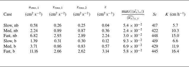
This approach leads to a dissipation estimate
 $8.8\times 10^{-5}$
m
$8.8\times 10^{-5}$
m
 $^2$
s−
$^2$
s−
 $^3$
and
$^3$
and
 $\tau _{\textit{SE}}$
estimate 0.10 s. The values of
$\tau _{\textit{SE}}$
estimate 0.10 s. The values of
 $\varepsilon$
calculated from sample records collected closest (
$\varepsilon$
calculated from sample records collected closest (
 $z/h=0.67$
) to the air–water interface are given in Appendix C.
$z/h=0.67$
) to the air–water interface are given in Appendix C.
4.3. Bulk gas transfer enhancement
The gas transfer velocity
 $K$
was enhanced by 15 %, 15 % and 9 % in the slow-, medium- and fast-flow-speed cases, respectively (see table 1 and figure 15). The gas transfer enhancement was greatest at the medium flow speed (
$K$
was enhanced by 15 %, 15 % and 9 % in the slow-, medium- and fast-flow-speed cases, respectively (see table 1 and figure 15). The gas transfer enhancement was greatest at the medium flow speed (
 $ \textit{Re}_h\approx 3\times 10^4$
). The
$ \textit{Re}_h\approx 3\times 10^4$
). The
 $K$
estimates based on DO measurements or calculated from SPIV images are presented in figure 15.
$K$
estimates based on DO measurements or calculated from SPIV images are presented in figure 15.
Gas transfer velocity
 $K$
estimates for cases with and without bars. The multiplicative constants used in the models were
$K$
estimates for cases with and without bars. The multiplicative constants used in the models were
 $C_{\textit{SE}}=0.25$
,
$C_{\textit{SE}}=0.25$
,
 $c=0.47$
and
$c=0.47$
and
 $c=0.40$
, for the SEM, the SDM without bars, and the SDM with bars, respectively. The error bars are based on 95 % confidence intervals from bias errors, such as in water depth and volume measurement in the case of directly measured
$c=0.40$
, for the SEM, the SDM without bars, and the SDM with bars, respectively. The error bars are based on 95 % confidence intervals from bias errors, such as in water depth and volume measurement in the case of directly measured
 $K$
, and velocity measurement via SPIV in the modelled
$K$
, and velocity measurement via SPIV in the modelled
 $K$
values.
$K$
values.

The root mean square error (RMSE) between the average gas transfer estimates (
 $\overline {\langle \hat {K}_{\textit{SEM}} \rangle _y }$
) based on the SEM, using TKE dissipation values calculated from the surface energy spectra, and directly measured values of bulk
$\overline {\langle \hat {K}_{\textit{SEM}} \rangle _y }$
) based on the SEM, using TKE dissipation values calculated from the surface energy spectra, and directly measured values of bulk
 $K$
, was 0.31 cm h−1 for cases without bars and 0.79 cm h−1 for cases with bars. For comparison, a similar approach was taken for the LEM (i.e.
$K$
, was 0.31 cm h−1 for cases without bars and 0.79 cm h−1 for cases with bars. For comparison, a similar approach was taken for the LEM (i.e.
 $K=C_{\textit{LE}}\sqrt {D_m\sqrt {\langle (v_s-\langle v_S\rangle _x)^2\rangle _x}/L_{22,1}}$
), where the multiplicative constant and error of this model were
$K=C_{\textit{LE}}\sqrt {D_m\sqrt {\langle (v_s-\langle v_S\rangle _x)^2\rangle _x}/L_{22,1}}$
), where the multiplicative constant and error of this model were
 $C_{\textit{LE}} = 1.05$
and
$C_{\textit{LE}} = 1.05$
and
 $ \textit{RMSE} = 1.2$
cm h−1 for cases without bars, and
$ \textit{RMSE} = 1.2$
cm h−1 for cases without bars, and
 $C_{\textit{LE}} = 0.96$
and
$C_{\textit{LE}} = 0.96$
and
 $ \textit{RMSE} = 1.7$
cm h−1 for cases with bars. This supports the theory that at high
$ \textit{RMSE} = 1.7$
cm h−1 for cases with bars. This supports the theory that at high
 $ \textit{Re}_t$
(i.e.
$ \textit{Re}_t$
(i.e.
 $\gt500$
), small eddy time scales are more representative of the renewal interval that impacts gas transfer rate than large eddy time scales are. Uncertainty in the directly measured
$\gt500$
), small eddy time scales are more representative of the renewal interval that impacts gas transfer rate than large eddy time scales are. Uncertainty in the directly measured
 $K$
values was 2 %, so 0.1–0.4 cm h−1, due to factors such as variation over the duration of an experiment, and uncertainty in the system’s interfacial area and volume (see (3.4)). The uncertainty in the SPIV-based gas transfer velocity
$K$
values was 2 %, so 0.1–0.4 cm h−1, due to factors such as variation over the duration of an experiment, and uncertainty in the system’s interfacial area and volume (see (3.4)). The uncertainty in the SPIV-based gas transfer velocity
 $\hat {K}_{\textit{SEM}}$
estimates was up to 3 %, largely due to the selection of
$\hat {K}_{\textit{SEM}}$
estimates was up to 3 %, largely due to the selection of
 $k$
bounds of the inertial subrange. Therefore, RMSE between the directly measured
$k$
bounds of the inertial subrange. Therefore, RMSE between the directly measured
 $K$
and
$K$
and
 $\hat {K}$
modelled from the SEM is less than the errors in the individual measurements only in the fast-flow-speed cases. The residual (
$\hat {K}$
modelled from the SEM is less than the errors in the individual measurements only in the fast-flow-speed cases. The residual (
 $|\hat {K}-K|$
) is greater than uncertainty in only 2 of the 6 cases, the slow- and medium-speed cases with bars. The error was less than if we used empirical constants from the literature, so more work to parametrise the empirical terms could further reduce error.
$|\hat {K}-K|$
) is greater than uncertainty in only 2 of the 6 cases, the slow- and medium-speed cases with bars. The error was less than if we used empirical constants from the literature, so more work to parametrise the empirical terms could further reduce error.
The multiplicative constant
 $C_{\textit{SE}}$
used in (2.13) to estimate
$C_{\textit{SE}}$
used in (2.13) to estimate
 $K$
from
$K$
from
 $S_{22,1}$
was set to 0.25 for cases with and without bars to minimise residuals from the directly measured values of
$S_{22,1}$
was set to 0.25 for cases with and without bars to minimise residuals from the directly measured values of
 $K$
. These values are lower than that proposed by Katul & Liu (Reference Katul and Liu2017) (
$K$
. These values are lower than that proposed by Katul & Liu (Reference Katul and Liu2017) (
 $\sqrt {2/15}$
) or those previously found empirically (e.g. 0.4). This is likely due to the complex influence of the channel secondary flows, such as anisotropy, lateral inhomogeneity, and other changes in TKE spectra due to production and transport of turbulence on scales different from those of standard open channel flow. For instance,
$\sqrt {2/15}$
) or those previously found empirically (e.g. 0.4). This is likely due to the complex influence of the channel secondary flows, such as anisotropy, lateral inhomogeneity, and other changes in TKE spectra due to production and transport of turbulence on scales different from those of standard open channel flow. For instance,
 $\varepsilon$
was estimated based on
$\varepsilon$
was estimated based on
 $S_{22,1}$
to help to account for anisotropy.
$S_{22,1}$
to help to account for anisotropy.
Another explanation for a discrepancy in
 $C_{\textit{SE}}$
across studies could be that certain assumptions that apply in the classical three-dimensional turbulence model may not hold in quasi-flat free-surface turbulence. For instance, Qi, Li & Coletti (Reference Qi, Li and Coletti2025) found that while the structure function scales similarly to dissipation rate in surface and subsurface turbulence (
$C_{\textit{SE}}$
across studies could be that certain assumptions that apply in the classical three-dimensional turbulence model may not hold in quasi-flat free-surface turbulence. For instance, Qi, Li & Coletti (Reference Qi, Li and Coletti2025) found that while the structure function scales similarly to dissipation rate in surface and subsurface turbulence (
 $D_{11}=C_{2s}(\varepsilon _sr)^{2/3}$
), the multiplicative constant
$D_{11}=C_{2s}(\varepsilon _sr)^{2/3}$
), the multiplicative constant
 $C_{2s}$
, analogous to
$C_{2s}$
, analogous to
 $\alpha$
in (4.7), was higher in free-surface turbulence than in three-dimensional turbulence. However, as long as
$\alpha$
in (4.7), was higher in free-surface turbulence than in three-dimensional turbulence. However, as long as
 $\alpha$
is constant over flow conditions, this should not reduce the accuracy of this SEM approach for estimating
$\alpha$
is constant over flow conditions, this should not reduce the accuracy of this SEM approach for estimating
 $K$
, as long as
$K$
, as long as
 $C_{\textit{SE}}$
could be adjusted to account for the change in
$C_{\textit{SE}}$
could be adjusted to account for the change in
 $\alpha$
.
$\alpha$
.
When applying the SEM, the multiplicative constant
 $C_{\textit{SE}}$
was not significantly different between cases with bars and without bars (
$C_{\textit{SE}}$
was not significantly different between cases with bars and without bars (
 $C_{\textit{SE}}=0.25$
,
$C_{\textit{SE}}=0.25$
,
 $R^2=0.978$
). When applying the SDM, the multiplicative constant
$R^2=0.978$
). When applying the SDM, the multiplicative constant
 $c$
was found to be higher when bars were not present (
$c$
was found to be higher when bars were not present (
 $c=0.5$
,
$c=0.5$
,
 $R^2=0.70$
) than when bars were present (
$R^2=0.70$
) than when bars were present (
 $c=0.4$
,
$c=0.4$
,
 $R^2=0.84$
); however, the difference was not statistically significant, due to the small sample size. The consistency, across cases with and without bars, of these multiplicative constants (
$R^2=0.84$
); however, the difference was not statistically significant, due to the small sample size. The consistency, across cases with and without bars, of these multiplicative constants (
 $c$
and
$c$
and
 $C_{\textit{SE}}$
) for models based on small-scale turbulence metrics suggests that the parameters that control gas transfer rate are consistent between cases with and without bars. The accuracy of the SEM suggests that CRSV enhance air–water gas transfer via small-scale turbulence; i.e. more small, fast eddies are produced in or transported upwards to the CBL, increasing the concentration gradient across the DSL.
$C_{\textit{SE}}$
) for models based on small-scale turbulence metrics suggests that the parameters that control gas transfer rate are consistent between cases with and without bars. The accuracy of the SEM suggests that CRSV enhance air–water gas transfer via small-scale turbulence; i.e. more small, fast eddies are produced in or transported upwards to the CBL, increasing the concentration gradient across the DSL.
4.4. Estimated spatial variability in gas transfer
In the cases with bars, the
 $C_{\textit{SE}}$
value is likely partially controlled by the proportion of high and low momentum pathway zones in the SPIV FOV. The normalised lateral fluctuations in gas transfer velocity estimates based on the SEM as a function of lateral position,
$C_{\textit{SE}}$
value is likely partially controlled by the proportion of high and low momentum pathway zones in the SPIV FOV. The normalised lateral fluctuations in gas transfer velocity estimates based on the SEM as a function of lateral position,
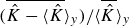 $(\overline {\hat {K}-\langle \hat {K}}\rangle _y)/\langle \overline {\hat {K}}\rangle _y$
, at the given flow speed, are shown in figure 16. For instance, in cases with bars,
$(\overline {\hat {K}-\langle \hat {K}}\rangle _y)/\langle \overline {\hat {K}}\rangle _y$
, at the given flow speed, are shown in figure 16. For instance, in cases with bars,
 $\overline {\hat {K}_{\textit{SEM}}}$
fluctuates around the spatial mean with amplitude approximately 10 % of the mean, and
$\overline {\hat {K}_{\textit{SEM}}}$
fluctuates around the spatial mean with amplitude approximately 10 % of the mean, and
 $\overline {\hat {K}_{\textit{SEM}}}$
has a much greater lateral variance in cases with bars: 0.20, 0.23 and 0.45 cm
$\overline {\hat {K}_{\textit{SEM}}}$
has a much greater lateral variance in cases with bars: 0.20, 0.23 and 0.45 cm
 $^2$
h−
$^2$
h−
 $^2$
in cases without bars, and 0.15, 0.44 and 0.83 cm
$^2$
in cases without bars, and 0.15, 0.44 and 0.83 cm
 $^2$
h−
$^2$
h−
 $^2$
in cases with bars and slow, medium and fast flow speeds, respectively. The lateral heterogeneity suggests that there are periodic fluctuations in gas transfer velocity, so the bounds of the FOV have a strong impact on the accuracy of
$^2$
in cases with bars and slow, medium and fast flow speeds, respectively. The lateral heterogeneity suggests that there are periodic fluctuations in gas transfer velocity, so the bounds of the FOV have a strong impact on the accuracy of
 $\hat {K}$
estimates based on surface renewal models. In these experiments, the SPIV FOV extends from the centreline of one bar to that of another (covering four bed bars), so the average
$\hat {K}$
estimates based on surface renewal models. In these experiments, the SPIV FOV extends from the centreline of one bar to that of another (covering four bed bars), so the average
 $\hat {K}$
estimate should represent the overall average.
$\hat {K}$
estimate should represent the overall average.
Normalised time-averaged
 $\hat {K}$
estimated using the SEM (using
$\hat {K}$
estimated using the SEM (using
 $S_{22,1}$
to estimate
$S_{22,1}$
to estimate
 $\varepsilon$
) as a function of lateral position, from SPIV measurement.The multiplicative constant used in the model was
$\varepsilon$
) as a function of lateral position, from SPIV measurement.The multiplicative constant used in the model was
 $C_{\textit{SE}}=0.25$
. The solid black line and right-hand axis indicate the bed elevation in cases with bars.
$C_{\textit{SE}}=0.25$
. The solid black line and right-hand axis indicate the bed elevation in cases with bars.

5. Conclusion
Laboratory experiments were conducted to measure gas transfer velocity in an open channel with and without longitudinal bed bars intended to stabilise CRSV. We found that the bed bars generated strong, stationary, depth-scale CRSV, as evidenced by the cross-stream (e.g. figure 4) and surface (e.g. figures 5 and 6) velocity fields. Analysis of the remote and in situ measurements within a pair of CRSV captures the lateral variation in Reynolds stresses (figure 12) and turbulent upwelling (figure 13) over the bars described by previous works (e.g. Nezu & Nakagawa Reference Nezu and Nakagawa1984; Anderson et al. Reference Anderson, Barros, Christensen and Awasthi2015; Vanderwel & Ganapathisubramani Reference Vanderwel and Ganapathisubramani2015). The in situ measurements also demonstrated the lateral gradient in normal Reynolds stress,
 $\partial \overline {u\prime v\prime }/\partial y$
, characteristic of these flows (Nezu & Nakagawa Reference Nezu and Nakagawa1984). Both in situ and remote velocity measurements indicate that turbulence anisotropy (e.g.
$\partial \overline {u\prime v\prime }/\partial y$
, characteristic of these flows (Nezu & Nakagawa Reference Nezu and Nakagawa1984). Both in situ and remote velocity measurements indicate that turbulence anisotropy (e.g.
 $\sqrt {\overline {v^{\prime 2}}}/\sqrt {\overline {u^{\prime 2}}}$
,
$\sqrt {\overline {v^{\prime 2}}}/\sqrt {\overline {u^{\prime 2}}}$
,
 $v_{\textit{rms},1}/u_{\textit{rms},1}$
and
$v_{\textit{rms},1}/u_{\textit{rms},1}$
and
 $L_{22,1}/L_{11,1}$
) tends to increase with flow speed and the presence of the bed bars. This anisotropy can make gas transfer prediction challenging because surface renewal models rely on quantification of near-surface vertical turbulent motions that are challenging to measure directly.
$L_{22,1}/L_{11,1}$
) tends to increase with flow speed and the presence of the bed bars. This anisotropy can make gas transfer prediction challenging because surface renewal models rely on quantification of near-surface vertical turbulent motions that are challenging to measure directly.
Remote measurements of the surface velocity demonstrated that these secondary flows increased the spatially averaged magnitude of the surface divergence by a factor 1.8–2.3, with peak divergence near the centreline of the bars, and peak convergence near the halfway point between bars. The spatial average of the temporal standard deviation of the surface divergence, which is representative of vertical turbulence intensity, increased by a factor 1.6–1.8 (figure 7). The percentage enhancement in surface divergence and other turbulence metrics tended to be highest in the medium- or fast-flow-speed cases, in which gas transfer enhancement was also strongest, suggesting that turbulence was enhanced by the mean flow energy more efficiently in cases with the established secondary flows than in the flat-bed case.
The auto-spectral density,
 $S_{11,1}$
,
$S_{11,1}$
,
 $S_{22,1}$
and
$S_{22,1}$
and
 $S_{22,2}$
, of the surface velocity also exhibits a shift in energy towards smaller scales and a bump in energy at scales close to the theoretical mixing length (e.g. Johnson & Cowen Reference Johnson and Cowen2016) that is larger than that detected in cases with a flat bed. This suggests that while the spanwise periodic velocity component is not included when calculating these energy spectra, the bed bars increase the intensity of bed-generated turbulent bursts with surface signature length scales near the Prandtl mixing length.
$S_{22,2}$
, of the surface velocity also exhibits a shift in energy towards smaller scales and a bump in energy at scales close to the theoretical mixing length (e.g. Johnson & Cowen Reference Johnson and Cowen2016) that is larger than that detected in cases with a flat bed. This suggests that while the spanwise periodic velocity component is not included when calculating these energy spectra, the bed bars increase the intensity of bed-generated turbulent bursts with surface signature length scales near the Prandtl mixing length.
Direct measurements of the dissolved tracer gas over time revealed that the presence of the bars increased the mean gas transfer velocity by 9–15 %. When using the power density spectra
 $S_{22,1}$
to calculate the TKE dissipation rate, the multiplicative constant used in the SEM,
$S_{22,1}$
to calculate the TKE dissipation rate, the multiplicative constant used in the SEM,
 $C_{\textit{SE}}$
, was found to be 0.25, compared to the empirical value 0.4 (ranging from 0.2 to 0.71) commonly found in previous studies. When applying the SDM, the multiplicative constant
$C_{\textit{SE}}$
, was found to be 0.25, compared to the empirical value 0.4 (ranging from 0.2 to 0.71) commonly found in previous studies. When applying the SDM, the multiplicative constant
 $c$
was less consistent across cases with and without bars than
$c$
was less consistent across cases with and without bars than
 $C_{\textit{SE}}$
, varying from 0.5 in cases without bars, to 0.4 in cases with bars. This suggests that the SDM may not capture all mechanisms by which the bed bars enhance gas transfer. For instance, the SDM considers turbulent fluctuations at all scales so would not capture the changes in the distribution of TKE across different scales (i.e. the shape of
$C_{\textit{SE}}$
, varying from 0.5 in cases without bars, to 0.4 in cases with bars. This suggests that the SDM may not capture all mechanisms by which the bed bars enhance gas transfer. For instance, the SDM considers turbulent fluctuations at all scales so would not capture the changes in the distribution of TKE across different scales (i.e. the shape of
 $S_{11,1}$
or
$S_{11,1}$
or
 $S_{22,1}$
). The SEM and the SDM consistently overestimated
$S_{22,1}$
). The SEM and the SDM consistently overestimated
 $K$
corresponding to the slowest flow case with bars, suggesting that the presence of the secondary flows may necessitate the use of a variable, rather than constant,
$K$
corresponding to the slowest flow case with bars, suggesting that the presence of the secondary flows may necessitate the use of a variable, rather than constant,
 $C_{\textit{SE}}$
that captures the impact of the bed forms on near-surface turbulence mixing across different Reynolds numbers.
$C_{\textit{SE}}$
that captures the impact of the bed forms on near-surface turbulence mixing across different Reynolds numbers.
Both measurement techniques highlight a need for careful instrument positioning, especially in the presence of CRSV that cause lateral inhomogeneity. As mentioned previously, the velocity field measurements suggest that there is stronger surface turbulence and TKE dissipation in the upwelling region over the bars, which theoretically leads to lateral variation in gas transfer velocity. The FOV of the remote sensing system was carefully positioned to extend from the centreline of one bar to that of another; however, such positioning may be more difficult in the field, when measuring gas transfer in the presence of CRSV. In the presence of CRSV, surface velocity measurements collected at the inflection point of the lateral velocity profile, or the centreline of a roller cell, were similar to the lateral average, as one might expect.
Overall, these results allow us to better understand and interpret single-point field measurements, which clearly depend on sampling location, especially in the cross-stream or cross-wind direction. The impact of these bed bars on turbulence and scalar transfer is also promising because it poses a potential passive low-energy method to strongly enhance stirring and interfacial exchange in flows.
Supplementary materials
Supplementary materials are available at https://doi.org/10.1017/jfm.2026.11247.
Acknowledgements
K.E.A. appreciates and acknowledges support from the American Association of University Women Dissertation Fellowship.
Funding
This research received no specific grant from any funding agency, commercial or not-for-profit sectors.
Declaration of interests
The authors report no conflict of interest.
Author contributions
K.E.A. performed formal analysis and wrote the original draft. E.A.C. contributed to the conceptualisation and methodology, and provided PIV analysis software, supervision, revision and editing. V.S. contributed to the conceptualisation and methodology, and performed experimental investigation.
Data availability statement
The data that support the findings of this study are available from the corresponding author, K.E.A., upon reasonable request.
Appendix A. Determination of gas transfer velocity
Dissolved oxygen was scavenged using cobalt (Co[II]) and sodium sulfite (Na
 $_2$
SO
$_2$
SO
 $_3$
) as prescribed by ASCE (2007). The system contains 15.73 m
$_3$
) as prescribed by ASCE (2007). The system contains 15.73 m
 $^3$
of water. We added 12.8 g of cobalt chloride hexahydrate (CoCl
$^3$
of water. We added 12.8 g of cobalt chloride hexahydrate (CoCl
 ${}_2{\cdot}$
6H
${}_2{\cdot}$
6H
 $_2$
O) once per water replacement to catalyse deoxygenation, and 1.456 kg of Na
$_2$
O) once per water replacement to catalyse deoxygenation, and 1.456 kg of Na
 $_2$
SO
$_2$
SO
 $_3$
before each re-aeration experiment to scavenge the DO (Citerone Reference Citerone2016).
$_3$
before each re-aeration experiment to scavenge the DO (Citerone Reference Citerone2016).
The saturation concentration was calculated according to the Benson & Krause (Reference Benson and Krause1984) parametrisation and the temperature values given in table 1):
 \begin{align} C_s(T) &= \exp\left [-a+\frac {b}{T}-\frac {c}{T^2}+\frac {d}{T^3}-\frac {e}{T^4}\right ] \!, \\[-10pt] \nonumber \end{align}
 \begin{align} a &= 139.34411, \\[-10pt] \nonumber \end{align}
 \begin{align} b &= 1.575701\times 10^5, \\[-10pt] \nonumber \end{align}
 \begin{align} c &= 6.642308\times 10^7, \\[-10pt] \nonumber \end{align}
 \begin{align} d &= 1.243800\times 10^{10}, \\[-10pt] \nonumber \end{align}
 \begin{align} e &= 8.621949\times 10^{11}. \\[9pt] \nonumber \end{align}
Here, we assumed a standard pressure of 1 atm. To confirm the validity of this assumption, barometric pressure measurements were collected (see table 3). Based on the Benson & Krause (Reference Benson and Krause1984) empirical pressure correction factor, deviations in barometric pressure from 1 atm led to relative error up to 1 % in
 $C_s$
(Citerone Reference Citerone2016). This error is accounted for in the overall error of the
$C_s$
(Citerone Reference Citerone2016). This error is accounted for in the overall error of the
 $K$
measurement, which is 2 %.
$K$
measurement, which is 2 %.
Mean barometric pressure during each flow case. Measurements were collected once per hour from the National Weather Service weather station at the Ithaca Tompkins Regional Airport (KITH - 42
 $^\circ$
29′27′′N, 76
$^\circ$
29′27′′N, 76
 $^\circ$
27′30′′W), 4 miles from, and 300 feet higher in elevation than, the laboratory location.
$^\circ$
27′30′′W), 4 miles from, and 300 feet higher in elevation than, the laboratory location.

Appendix B. Phase wrapping correction
See Rusello (Reference Rusello2009) for a description of phase wrapping. Nortek guidelines were used to correct the phase velocity by transforming the velocity vectors into beam coordinates, identifying the wrapped values, and adding a multiple of the ambiguity velocity to those wrapped values:
 \begin{align} u_{\textit{corrected}} = u_{w\textit{rapped}}+\frac {c_s}{f \Delta t}, \end{align}
where
 $c_s$
is the speed of sound in water (1483.3 m s−1),
$c_s$
is the speed of sound in water (1483.3 m s−1),
 $f$
is the acoustic frequency (
$f$
is the acoustic frequency (
 $10^7$
Hz), and
$10^7$
Hz), and
 $\Delta t$
is the lag time (
$\Delta t$
is the lag time (
 $1.6\times 10^{-4}$
s).
$1.6\times 10^{-4}$
s).
Appendix C. Local turbulence metrics from in situ measurements
For reference, local turbulence statistics from six subsurface sample locations around a pair of bed bars (centred at
 $y/h= 0$
and 2) and three flow speeds are shown in table 4. The main source of error in this
$y/h= 0$
and 2) and three flow speeds are shown in table 4. The main source of error in this
 $\varepsilon$
estimate is due to selection of the flat region. Reasonable variation in the selected bounds of the inertial subrange contributes
$\varepsilon$
estimate is due to selection of the flat region. Reasonable variation in the selected bounds of the inertial subrange contributes
 $\pm$
0.2 cm h−1 error (95 % confidence interval, unless otherwise stated) in the
$\pm$
0.2 cm h−1 error (95 % confidence interval, unless otherwise stated) in the
 $K$
estimate. The turbulent Reynolds number is greater than 500, so we would expect small eddies to dominantly control
$K$
estimate. The turbulent Reynolds number is greater than 500, so we would expect small eddies to dominantly control
 $K$
.
$K$
.
Local turbulence statistics from six sample locations at
 $z/h= 0.67$
around a pair of bed bars (centred at
$z/h= 0.67$
around a pair of bed bars (centred at
 $y/h = 0$
and 2) and three flow speeds (
$y/h = 0$
and 2) and three flow speeds (
 $U_s = 16.4$
, 29.7 and 53.9 cm s−1). Here,
$U_s = 16.4$
, 29.7 and 53.9 cm s−1). Here,
 $y/h$
is measured from the centreline of the fourth bar (
$y/h$
is measured from the centreline of the fourth bar (
 $9h$
from the nearest side wall).
$9h$
from the nearest side wall).


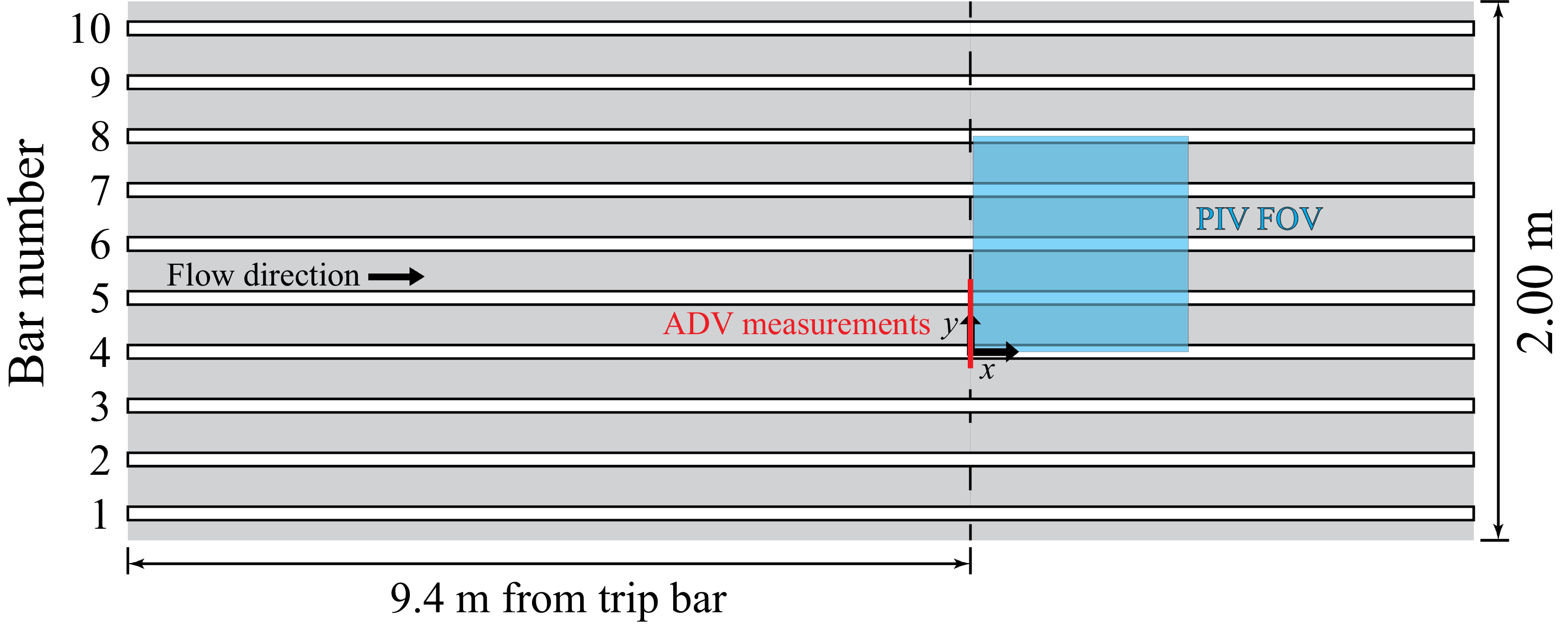
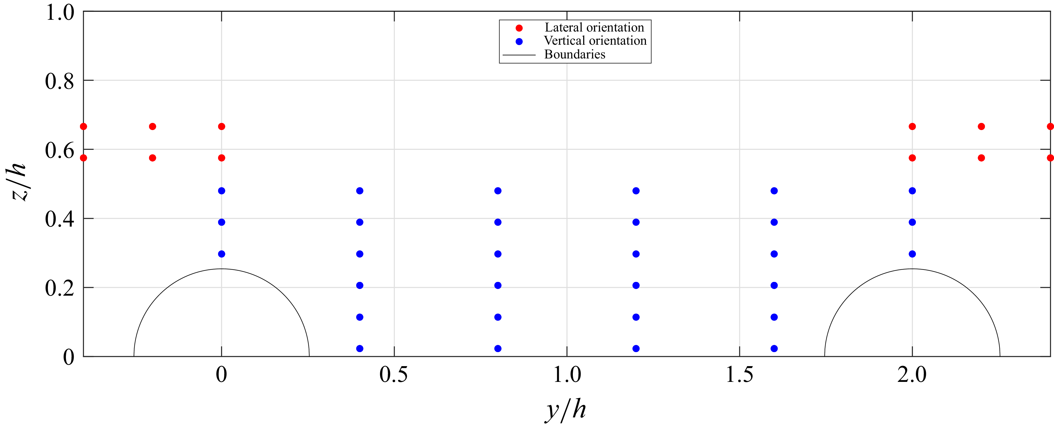


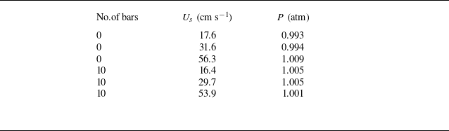


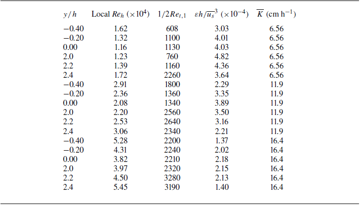


 Open access