

Introduction
Broad-scale studies of the North American megafaunal extinction have historically relied on geographic binning according to modern human or biotic boundaries. Current common practices for evaluating radiocarbon dates of extinction events use two-dimensional graphs and plots divided by modern boundary lines—states, countries, or regions—that do not reflect Pleistocene biomes (i.e., Barnosky et al. Reference Barnosky, Koch, Feranec, Wing and Shabel2004; Johnson et al. Reference Johnson, Bradshaw, Cooper, Gillespie and Brook2013; Lima-Ribeiro and Felizola Diniz-Filho Reference Lima-Ribeiro and Felizola Diniz-Filho2013; Boulanger and Lyman Reference Boulanger and Lyman2014). Binning is practical, as humans and megafauna rarely died in the same place, and so testing whether they did or did not coexist requires some geographic flexibility. However, bin size and shape greatly affect interpretation of a distribution, as can be seen when interpreting continuous data using histograms. Hence it should be of little surprise that research on the interactions between humans and megafauna across the North American continent is often contradictory, with some concluding general overlap (Barnosky et al. Reference Barnosky, Koch, Feranec, Wing and Shabel2004; Surovell et al. Reference Surovell, Waguespack and Brantingham2005; Johnson et al. Reference Johnson, Bradshaw, Cooper, Gillespie and Brook2013) and others concluding that humans and megafauna never temporally overlapped (Lima-Ribeiro and Felizola Diniz-Filho Reference Lima-Ribeiro and Felizola Diniz-Filho2013).
These divergent views limit the scientific work evaluating extinction drivers. In North America in particular, human immigration occurs during the same 5000-year window as rapid climate change. Sorting out the particular effects of each on megafaunal populations could yield important information regarding the fate of large mammals in the ongoing Anthropocene extinctions (Diamond Reference Diamond1989; Faith and Surovell Reference Faith and Surovell2009). The many hypotheses explaining the cause of this megafaunal extinction primarily revolve around human and/or climate drivers. Human-driven extinction scenarios include illness introduced by humans and their commensals (Fiedel Reference Fiedel2005), environmental perturbation by human-induced change in the trophic cycle (sitzkrieg) (Diamond Reference Diamond1989), cascading trophic interactions by humans placing slow strain on megafaunal populations (Jones et al. Reference Jones, Beck, Nials, Neudorfer, Brownholtz and Gilbert1996; Ripple and Van Valkenburgh Reference Ripple and Van Valkenburgh2010), and rapid overhunting as humans reached carrying capacity (blitzkrieg) (Martin Reference Martin1984). Climatically driven extinction scenarios relate to environmental disruption in the wake of the abrupt cooling and subsequent warming of the Younger Dryas (Alley Reference Alley2000; Fiedel Reference Fiedel2011). Previous workers have invoked the coincidence between Younger Dryas cooling and initial human colonization, suggesting that it is possible that both climate and human pressures played a role in forcing the extinction, but the latest evidence (e.g., Braje and Erlandson Reference Braje and Erlandson2013) suggests that human pressures can take longer to cause extinction than previously anticipated. As radiocarbon dating has become more precise and more prevalent, tests of these various hypotheses have become more refined (Barnosky et al. Reference Barnosky, Koch, Feranec, Wing and Shabel2004; Johnson et al. Reference Johnson, Bradshaw, Cooper, Gillespie and Brook2013; Lima-Ribeiro and Felizola Diniz-Filho Reference Lima-Ribeiro and Felizola Diniz-Filho2013; Mann et al. Reference Mann, Groves, Kunz, Reanier and Gaglioti2013) yet have still been hindered by a traditional reliance on geographic binning.
Here we use a geospatially explicit approach incorporating published radiocarbon dates to interpolate two surfaces: a last-appearance datum (LAD) surface for megafauna and a first-appearance datum (FAD) surface for humans. Creating surfaces rather than creating artificial geographic bins allows us to simultaneously evaluate geographic and temporal trends and better test the full suite of Pleistocene extinction hypotheses. If blitzkrieg were the dominant trend, then FADs and LADs should follow each other extremely closely, producing fewer than 1200 years between first FAD and final LAD as predicted for an overhunting scenario by Alroy (Reference Alroy2001). Sitzkrieg and intensification scenarios would show greater lag time (in some cases up to 50,000 years, as discussed by Prowse et al. [Reference Prowse, Johnson, Bradshaw and Brook2014]), and if influenced equally by biases in preservation, identification, and collecting effort, the FAD and LAD maps should broadly resemble one another. Disease would either appear as a geologically instantaneous LAD surface or as a spreading wave of LAD surface from the point of initial human occupation. As humans would only need to be an initial disease vector, and megafauna themselves could continue to spread the disease on their own, disease would appear as an instantaneous interpolated surface without regard to younger FAD surfaces. Finally, under the simple model that climate cooling from the onset of the Younger Dryas (12,900 calibrated years before present [cal yr BP]) or warming from the end of the Older Dryas (14,600 cal yr BP) was the single cause of megafaunal extinction, the results should show LAD surfaces that fall into the Younger Dryas period. These surfaces should also show a rough latitudinal gradient, with northern latitudes experiencing an earlier influence of climate change (Shuman et al. Reference Shuman, Webb, Bartlein and Williams2002; Strong and Hills Reference Strong and Hills2005; Shakun et al. Reference Shakun, Clark, He, Marcott, Mix, Liu, Otto-Bliesner, Schmittner and Bard2012).
Materials and Methods
Radiocarbon Data
We used radiocarbon dates of Pleistocene bones and associated organic material from recent literature (Barnosky et al. Reference Barnosky, Barnosky, Nickmann, Ashworth, Schwert and Lantz1988; Jones et al. Reference Jones, Beck, Nials, Neudorfer, Brownholtz and Gilbert1996; Robinson et al. Reference Robinson, Pigott Burney and Burney2005; Steadman et al. Reference Steadman, Martin, MacPhee, Jull, McDonald, Woods, Iturralde-Vinent and Hodgins2005; Surovell et al. Reference Surovell, Waguespack and Brantingham2005; Arroyo-Cabrales et al. Reference Arroyo-Cabrales, Polaco and Johnson2006; Guthrie Reference Guthrie2006; Robinson et al. Reference Robinson, Ort, Eldridge, Burke and Pelletier2009; Schubert Reference Schubert2010; Waters et al. Reference Waters, Stafford, McDonald, Gustafson, Rasmussen, Cappellini, Olsen, Szklarczyk, Jensen and Gilbert2011; Lima-Ribeiro and Felizola Diniz-Filho Reference Lima-Ribeiro and Felizola Diniz-Filho2013; Boulanger and Lyman Reference Boulanger and Lyman2014) and the Paleoindian Database (Anderson et al. Reference Anderson, Miller, Yerka, Gillam, Johanson, Anderson, Goodyear and Smallwood2010) and Canadian Archeological Radiocarbon Database (Gajewski et al. Reference Gajewski, Munoz, Peros, Viau, Morlan and Betts2011). We used several criteria to discard potentially unreliable dates. First, we discarded radiocarbon dates that used apatite, as these are frequently inaccurate (Hassan and Ortner Reference Hassan and Ortner1977); dates that relied on radiometric dates stratigraphically removed from megafaunal or confirmed human occurrences; and dates that had high measurement uncertainty (>6%). We also discarded dates for Bison species, as there is evidence that extinct Bison taxa evolved into modern taxa or only went extinct recently (Guthrie Reference Guthrie1970). We included Rangifer dates only in areas that are not part of their modern historical range. We preferentially used carbon accelerator mass spectrometry or XAD (industrial designation for filter material) dates (Kirner et al. Reference Kirner, Burky, Taylor and Southon1997). For specimens with multiple dates, we averaged the dates before calibration, then calculated a summary uncertainty for the average by taking the square root of the sum of the squares of the standard errors (called summing in quadrature, or error propagation) and dividing by the number of dates, a procedure derived from the rules for propagating error for subtraction and addition in Taylor (Reference Taylor1997). We calibrated the 1 sigma calendar age of the dates using the IntCal13 calibration curve (Reimer et al. Reference Reimer, Bard, Bayliss, Beck, Blackwell, Bronk Ramsey, Buck, Cheng, Edwards, Friedrich, Grootes, Guilderson, Haflidason, Hajda, Hatte, Heaton, Hoffman, Hogg, Hughen, Kaiser, Kromer, Manning, Niu, Reimer, Richards, Scott, Southon, Staff, Turney and van der Plicht2013) in the OxCal program created by the Oxford Radiocarbon Accelerator Unit (Bronk Ramsey and Lee Reference Bronk Ramsey and Lee2013). Following established procedures (Bronk Ramsey Reference Bronk Ramsey1995, Reference Bronk Ramsey2001), we calculated a mean calibrated age for each date by averaging the upper and lower 95% confidence limits derived from the OxCal calibration.
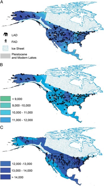
We then culled dates to remove local temporal outliers that were clearly not first appearances of humans or last appearances of megafauna, discarding dates within 1.5 decimal degrees of a reliable older FAD or younger LAD (Supplementary Table S1). We also removed LAD data from underneath the approximate extent of the Laurentide and Cordilleran ice sheets at the onset of the study interval, 15,000 cal yr BP (Barnosky et al. Reference Barnosky, Holmes, Kirchholtes, Lindsey, Maguire, Poust, Stegner, Sunseri, Swartz, Swift, Villavicencio and Wogan2014), as the temporal disparity and poor sampling of these last-appearance data created high uncertainty throughout the map. No FAD data points were present underneath the extent of the ice sheet. The initial data set consisted of 243 published possible LADs and 221 published possible FADs. After the data were pruned, the final data set included 95 LADs (12,980 to 7,917 cal yr BP) and 75 FADs (15,739 to 8,730 cal yr BP) (Supplementary Tables S2 and S3) and covered the continent exposed during the Last Glacial Maximum (Fig. 1).
Kriged event surfaces for human first appearance and megafaunal last appearance. A, Bayesian kriging LAD surface with LAD localities. B, Ordinary kriging LAD surface with LAD localities. C, Ordinary kriging FAD surface with FAD localities.
The complete data set uses radiocarbon dates from the remains of several orders of mammals, each of which may have been affected differently during the extinction. To see whether trends differed among these orders, we subsampled the original LAD data set at the finest taxonomic level possible. Many taxa were rare, so we divided the data into groupings of Mammuthus, Mammut, Equus, and Artiodactyla to maximize the data subsets. We then pruned the data set for each of these orders using the radiocarbon standards described earlier.
Kriging Methodology
Kriging is an interpolation algorithm that creates an estimated surface of the mean value of point data, using the spatial autocorrelation of the point data to adjust for trends (Zimmerman and Zimmerman Reference Zimmerman and Zimmerman1991). We used kriging to create interpolation surfaces of human FADs and megafaunal LADs, and from these produced a map of human–megafaunal overlap duration. We created models in ArcGIS using four variants of kriging: simple, ordinary, universal, and empirical Bayesian kriging. Each model type interpolates with its own assumptions: simple kriging interpolates without assuming that any additional trends in the data are present; ordinary kriging assumes that regional trends overwhelm local variation; universal assumes that an overarching trend (i.e., a north to south wave or radiating bands from a single region) is present throughout the whole map; and empirical Bayesian kriging finds the most likely model to predict a given data set, which could incorporate any or all of the trend aspects of simple, ordinary, or universal kriging (Kleijnen Reference Kleijnen2009). Because each kriging technique best fits a different local, regional, or continent-wide pattern, the type of model that best fits the data also reveals the nature of the data. Following standard model-selection procedures (as per Johnston et al. Reference Johnston, Ver Hoef, Krivoruchko and Lucas2001), we selected models that had the smallest root-mean-squared (RMS) prediction error, an average standard error nearest the RMS prediction error, a standardized mean nearest to zero, a standardized RMS prediction error near 1, and low uncertainty across the study area. Models frequently were not superior in all five criteria; we chose the models that had best performance in as many criteria as possible (Supplementary Table S4). ArcGIS provides prediction estimation uncertainties for all kriged surfaces, but both the LAD and the FAD uncertainties needed to be accounted for in the overlap map. Because the underlying math of the overlap surface was simple subtraction (FAD−LAD), we could combine (or propagate) the certainty by taking the square root of the sum of the variances of the two surfaces: ${\rm SE}\left( {{\rm FAD}\,{\minus}\,{\rm LAD}} \right){\equals}<$> <$>\sqrt {{\rm Var}\left( {{\rm FAD}} \right){\plus}{\rm Var}\left( {{\rm LAD}} \right)} $
. This calculation (also called summing in quadrature) provides a 68% confidence interval on the overlap surface (FAD−LAD), which we multiplied by 1.96 to create a 95% confidence interval (Taylor Reference Taylor1997).
${\rm SE}\left( {{\rm FAD}\,{\minus}\,{\rm LAD}} \right){\equals}<$> <$>\sqrt {{\rm Var}\left( {{\rm FAD}} \right){\plus}{\rm Var}\left( {{\rm LAD}} \right)} $
. This calculation (also called summing in quadrature) provides a 68% confidence interval on the overlap surface (FAD−LAD), which we multiplied by 1.96 to create a 95% confidence interval (Taylor Reference Taylor1997).
Calibrated radiocarbon dates are a complex probability distribution that we summarized using the mean and standard deviation of the distribution, though this is a simplification of the statistical reality (Telford et al. Reference Telford, Heegaard and Birks2004). For the purposes of this analysis, we specified a uniform date uncertainty of 10% in the kriging models. This value is larger than the actual uncertainty of included dates (because we used a 6% cutoff for observed date uncertainty) but gives the model more flexibility in adjusting around radiocarbon means to find a robust surface.
Our method does not account for the uncertainty in extinction events that arises from sampling bias. Current methods to incorporate sampling bias calculate uncertainty in FAD/LAD values using sampling distributions through time and therefore require multiple dates at a single locality (Marshall Reference Marshall1994, Reference Marshall1997); such data were not available at most of the localities, and so we could not directly incorporate the sampling uncertainty in this study. Other studies suggest that actual extinctions trail LADs by 700 to 1000 years (Barnosky et al. Reference Barnosky, Lindsey, Villavicencio, Bostelmann, Hadly, Wanket and Marshall2015) but can range up to 2400 years (Bradshaw et al. Reference Bradshaw, Cooper, Turney and Brook2012). Because we did not have the data to calculate site-specific extinction sampling bias, we relied on these previously published estimates. The surfaces should therefore not be interpreted as representing the precise time of an extinction or arrival but only as an interpolated surface of the last or first appearance in the fossil record. The propagated uncertainty can be perceived as a two-tailed distribution, but the additional underlying sampling uncertainty is only right-tailed for LADs and left-tailed for FADs: that is, extinctions likely occurred later than the LAD surface, and arrivals likely occurred earlier than the FAD surface. Because the core of our question is about overlap between humans and megafauna, comparison of LAD and FAD surfaces gives us a conservative test. That is, if we find evidence of an overlap in appearance data, we can have confidence that the actual time of overlap was larger. Similarly, areas with apparent disjunction of less than 2000 years may not be true areas of nonoverlap between humans and megafauna.
Results
First- and Last-Appearance Surfaces
Both the FAD and LAD surfaces (Fig. 1A–C) produced predictions with uncertainty in interpolation that were approximately equivalent to the measured uncertainty in the original radiocarbon dates (Supplementary Fig. S1).
The LAD surface was best modeled by two of the kriging models, neither of which was objectively better than the other. Ordinary kriging with a second-order trend removal and a Box-Cox transformation of two more accurately fit the young data but had higher uncertainty (Fig. 1B). Bayesian kriging with an empirical log function to correct for nonnormality in the data did not accurately predict the young dates but had much lower uncertainty and better overall fit (Fig. 1C). Regardless of kriging model, the differences in regional trends were greater than 1 SE in surface prediction (Supplementary Fig. S1). LADs were generally older at higher latitudes, but LADs were considerably more recent in Mexico and southern Texas, Tennessee, and the Great Lakes region (Fig. 1B). When subdivided by taxa, the last-appearance surface shows that the more recent LADs are primarily occurrences of Mammuthus (Supplementary Fig. S2). The predominance of late-occurrence Mammuthus may result from sampling bias, as even midsection chunks of bone can be identified as proboscidean. Late LADs of Mammuthus abundance may also reflect extinction resistance, which has been predicted for proboscideans by Alroy (Reference Alroy2001). Regardless, our LAD surface is likely more accurate for proboscideans than for less-sampled megafauna. Though Mammuthus were present across the continent during the end of the Pleistocene, the most recent dates for Mammut were highly clustered in the northeastern United States. The Mammut diet had a high proportion of leaves, bark, and twigs (Green et al. Reference Green, Semprebon and Solounias2005) and was more browsing dependent than the mixed-feeding to grazing diet of Mammuthus (Rivals et al. Reference Rivals, Semprebon and Lister2012). Vegetation reconstructions of the shrinking eastern expanse of the cool mixed forest biome from 16,000 cal yr BP to about 5000 cal yr BP (Williams et al. Reference Williams, Shuman, Webb, Bartlein and Leduc2004) correspond to the limited range of Mammut during the extinction event, and so diet and habitat requirements may explain Mammut’s restricted range at the end of the Pleistocene.
The most accurate FAD surface employed ordinary kriging with a second-order trend (Zimmerman and Zimmerman Reference Zimmerman and Zimmerman1991). Because ordinary kriging works best when trends are regional rather than continent-wide, the success of ordinary kriging implies a highly regional aspect to initial human appearances (Fig. 1C). The difference between the older regions of first appearance and the remainder of the continent was larger than the 95% uncertainty interval in surface prediction (Supplementary Fig. S1) and therefore unlikely to be a statistical artifact. The two older FAD areas were (1) from the Great Lakes region to the southeastern United States and (2) the Pacific Northwest, adjacent to both presumed pathways from Beringia (Steele et al. Reference Steele, Adams and Sluckin1998; Anderson and Gillam Reference Anderson and Gillam2000; Bradley and Stanford Reference Bradley and Stanford2004).
Overlap Surface
The length of co-occupation indicated by the overlap surface (FAD − LAD) was highly regional in nature (Fig. 2 A,B). In Alaska, megafauna had disappeared from the fossil record 1000 to 4000 years before human occupation, while in the Great Lakes region, humans and megafauna coexisted for at least 7000 years (according to the less conservative ordinary kriging model) or 3000 years (according to the more conservative Bayesian model). The propagated 95% uncertainty interval in regions of the overlap surface was larger than the predicted overlap between megafauna and humans regardless of which model was used, but the tight correlation between megafaunal extinction and human arrival was likely distorted by sampling bias, which causes a lag between LAD and extinction and between human arrival and first appearance (Marshall Reference Marshall1994). To examine this, we also interpreted the results by incorporating a 700-year buffer before FADs and after LADs to match the estimated mean interval between LAD and extinction reported by Barnosky et al. (Reference Barnosky, Lindsey, Villavicencio, Bostelmann, Hadly, Wanket and Marshall2015) (Supplementary Fig. S4). With these very broad confidence intervals incorporated, everywhere on the continent showed some overlap, except Alaska.
Overlap between human first appearance and megafaunal last appearance using (A) ordinary kriging for the LAD map and (B) Bayesian kriging for the LAD map. The small maps are the same as the larger maps but are overlaid with a translucent gray shading to indicate where the 68% and 95% confidence intervals (1 SE and 2 SE) have uncertainty greater than the overlap trend.

Discussion
Model Choice
An advantage of kriging over other interpolation methods is its weighting scheme, which counterbalances unusually young or old dates by pulling the predicted surface according to trends dictated by neighboring data points. Because of this weighting scheme, the method was robust to pull by erroneously young dates. However, the Bayesian model resisted young dates to the point of being inflexible, overpredicting the age of young LAD dates by several thousand years. Ordinary kriging fit the younger data better yet had high prediction uncertainty because of the heterogeneity of the surface, while the prediction homogeneity of the Bayesian model had lower uncertainty (Fig. 1A,B). We included both models for comparison. Though the predicted surfaces differ in numerical value, they do not differ in overall trend and differ only minimally in predicted overlap between last megafaunal appearance and first human appearance (Fig. 2).
Human Arrival and Dispersal
Recent research shows that human migration onto the continent occurred in multiple waves, with the most accepted early-dispersal pathway being along the Pacific Coast (Goebel et al. Reference Goebel, Waters and O’Rourke2008; Reich et al. Reference Reich, Patterson, Campbell, Tandon, Mazieres, Ray, Parra, Rojas, Duque and Mesa2012; Anderson et al. Reference Anderson, Bissett, Yerka, Graf, Ketron and Waters2013). Our model hindcasts the oldest signs of human appearance as a swath stretching from Florida to the Great Lakes. The minimal support for the older Pacific Coast surface in our model may be in part a preservation bias, as Holocene sea-level rise may have obscured older coastal sites (Anderson and Gillam Reference Anderson and Gillam2000; Lambeck and Chappell Reference Lambeck and Chappell2001; Anderson et al. Reference Anderson, Bissett, Yerka, Graf, Ketron and Waters2013). The older surface from the Great Lakes to Florida is supported by significantly more data, but matches no known postulated dispersal route—indeed, even the disputed North Atlantic ice-edge corridor (or Solutrean) hypothesis (Bradley and Stanford Reference Bradley and Stanford2004; Eren et al. Reference Eren, Patten, O’Brien and Meltzer2013) does not match our predicted surface, as the northeastern states lack any signs of older occupation. Our model indicates that hypothetical Solutrean immigrants would not have moved inland until reaching North Carolina, despite passing significant sections of habitable land farther north. Even if, as in the Pacific, older sites have been obscured on the Atlantic coastline by Holocene sea-level rise, there should have been a connection between the northern coast and the older inland surface. The older swath of data found between Florida and the Great Lakes cannot be explained by the North Atlantic ice-edge corridor hypothesis in its current form, but it also cannot be explained by the Bering land-bridge hypothesis; instead, our model predicts a secondary time period of initial occupation of about 12,000calyrBP through the ice-free corridor, which matches closely with when the ice-free corridor became habitable (Pedersen et al. Reference Pedersen, Ruter, Schweger, Friebe, Staff, Kjeldsen, Mendoza, Beaudoin, Zutter and Larsen2016).
Though the overall FAD surface showed humans spread across the continent over 3000 years, almost 50% of the appearance surface was concentrated between 13,500 and 13,000 cal yr BP. The distribution of dates (Figs. 1C, 3) indicates that human movement across the continent began slowly, with the oldest 25% of dates stretching across almost 1500 years but dramatically accelerating after 13,500 cal yr BP. This pattern of rapid population dispersal is consistent with Alroy’s (Reference Alroy2001) numerical model of human settlement of the continent.
Histograms of dates reconstructed for FAD and LAD surfaces, above Greenland ice-core temperature reconstructions for this interval (Alley Reference Alley2000). Solid vertical lines highlight the Younger Dryas cooling interval (12,900 to 11,650 cal yr BP).

Testing Previous Hypotheses
Our adoption of an explicit spatial framework produced a regionally and temporally explicit view of the North American megafaunal last appearances for the reevaluation of hypothesized causes of the extinction.
A blitzkrieg model of overhunting has been predicted to take between 800 and 1600 years after human arrival (Alroy Reference Alroy2001), but our overlap results took place over 3000–5000 years, inconsistent with a continental-scale blitzkrieg. Several areas of our model had reconstructed overlap of 3000 years or more, inconsistent with a localized blitzkrieg. Furthermore, many areas with low or no overlap were also areas with poor sampling, particularly the West Coast, where sea-level rise likely obscured older coastal sites. Additionally, the quantitative model of human-mediated extinction (Alroy Reference Alroy2001) predicted that extinctions should only follow in the wake of human population reaching carrying capacity, but we found no large-scale correlation between human arrival time and date of last local appearance (Fig. 2A,B). The extinction of megafauna may have taken place over a time span similar to that of human occupation, but human first appearance and megafaunal last appearance did not follow one another in a correlated fashion across the landscape. Consequently, we cannot support the blitzkrieg hypothesis that human settlement directly caused a rapid megafaunal extinction process across the continent. However, much of the western United States did show between 800 and 1600 years of overlap in appearance surfaces, so localized blitzkrieg effects may have occurred in some areas (but see the “Materials and Methods” discussion of extinction lag behind LADs and arrival before FADs).
The pattern of last appearance was also inconsistent with commensally introduced disease (Fiedel Reference Fiedel2005), which would have produced either a monotonic wave of LADs spreading from an origination point or an extinction surface uniform at the resolution of these radiocarbon dates. Similarly, the results were inconsistent with extinction driven by technological advancement. Previous studies have shown that the spread of Clovis technology was nearly instantaneous at 12,800calyrBP (Hamilton and Buchanan Reference Hamilton and Buchanan2007; Waters and Stafford Reference Waters and Stafford2007), but the reconstructed last-appearance surface is not instantaneous at or after this date (Figs. 1, 3). It is unlikely that the rapid spread of Clovis technology was a key driver continent-wide, although it could have had a large impact in some areas (Jenkins et al. Reference Jenkins, Davis, Stafford, Campos, Hockett, Jones, Cummings, Yost, Connolly, Yohe and Gibbons2012).
A slower style of human-caused extinction has been hypothesized as a result of cascading changes in trophic levels (Fisher Reference Fisher1996, Reference Fisher2009; Fox and Fisher Reference Fox and Fisher2001; Ripple and Van Valkenburgh Reference Ripple and Van Valkenburgh2010): humans were a predator introduced into the system that caused a restructuring of predator–prey relations, destabilizing vulnerable species into eventual extinction. This slower human influence, called the sitzkrieg hypothesis, would have been geographically amorphous, save that it would have required considerable overlap between humans and megafauna. Recent work has demonstrated that human populations may have had an even slower detrimental influence on animal populations than previously estimated: in Australia, humans arrived 50,000yearsBP, and their slow population growth caused multiple species to go extinct as late as the Holocene (Prowse et al. Reference Prowse, Johnson, Bradshaw and Brook2014). Similarly, hunting over the course of 8000 years led to the eventual extinction of the flightless sea duck from California coastlines (Jones et al. Reference Jones, Porcasi, Erlandson, Dallas, Wake and Schwaderer2008). Our predicted surfaces do not reject the possibility of a local increase in human population leading to an eventual extinction or the cascading trophic changes that human introduction may have caused; several areas of the maps show thousands of years of overlap, consistent with intensification or sitzkrieg as an eventual extinction driver.
The Younger Dryas cooling event (12,900–11,650 cal yr BP) (Alley Reference Alley2000) captures 67–79% (ordinary vs. Bayesian) of last-appearance surface values (Figs. 1, 3, and Supplementary Fig. S3). However, the LAD surface was highly regional and therefore inconsistent with cooling as a sole extinction driver. Were climatic cooling the predominant cause of the megafaunal last appearances, the LAD map would have been either best modeled by a universal kriging function (Kleijnen Reference Kleijnen2009), creating a surface dominated by an overarching trend from north to south according to a thermal gradient, or the surface would have occurred within the time span of the Younger Dryas. There was no universal trend in either LAD surface: though the colder northern areas had older extinctions, the middle of the continent had high regional variation despite thorough data sampling. While climate cooling likely had an effect, particularly in northern latitudes (where megafauna went extinct before humans arrived), other processes mediated the extinctions in lower latitudes. Both kriged models predict last appearances during the period of abrupt warming after the Younger Dryas—in some areas heating as well as cooling may have been detrimental (Fig. 3, and Supplementary Fig. S3).
Our last-occurrence surfaces broadly correspond to previous research on regional changes in biomes and precipitation. As the climate continued warming toward the beginning of the Holocene, Pleistocene biomes migrated northward (Shuman et al. Reference Shuman, Webb, Bartlein and Williams2002; Williams et al. Reference Williams, Shuman, Webb, Bartlein and Leduc2004; Strong and Hills Reference Strong and Hills2005). In the Great Lakes, biome response seems to have trailed climatic events by a 400-year lag (Gonzales and Grimm Reference Gonzales and Grimm2009). Though this estimate falls within an uncertainty interval normal for radiocarbon dates and is smaller than the predicted pollen accuracy interval of 500 years (Blois et al. Reference Blois, Williams, Grimm, Jackson and Graham2011), it is still likely that biomes did not immediately and uniformly respond to the temperature change recorded in Greenland. Temperature and precipitation changes varied by latitude and ocean proximity, so climate did not uniformly change across North America (Shuman et al. Reference Shuman, Webb, Bartlein and Williams2002; Strong and Hills Reference Strong and Hills2005; Shakun et al. Reference Shakun, Clark, He, Marcott, Mix, Liu, Otto-Bliesner, Schmittner and Bard2012). The Younger Dryas cold period itself was only discernible in the Northern Hemisphere and was more pronounced at higher latitudes (Shakun et al. Reference Shakun, Clark, He, Marcott, Mix, Liu, Otto-Bliesner, Schmittner and Bard2012).
Our last-appearance model surfaces were heterogeneous in nature, following larger regional patterns but not conforming to a single latitudinal gradient. In the Great Basin region, our models predict extinctions that match large changes in the local hydrological cycle, occurring concurrently with regression of regional lake systems, such as Lake Gilbert (Benson et al. Reference Benson, Currey, Dorn, Lajoie, Oviatt, Robinson, Smith and Stine1990; Oviatt Reference Oviatt2014). Most of the Alaskan extinction surface corresponds to the Younger Dryas, which in turn was marked by an increase in local precipitation and turnover from a dry mammoth steppe to a wetter taiga–tundra ecosystem (Guthrie Reference Guthrie2006). Of greatest interest are the areas with unusually recent last appearances, as they may represent refugia, areas insulated against the more extreme climate changes of northern latitudes. These surfaces, too, match with unique precipitation and biotic changes: from 11,000 to 10,000 cal yr BP, an influx of tropical storms from the eastern Pacific Ocean led to higher precipitation in Mexico and southern Texas, with a no-analogue Pleistocene biome most comparable to modern southern Idaho (Metcalfe et al. Reference Metcalfe, O’Hara, Caballero and Davies2000; Hall and Goble Reference Hall and Goble2012; Lyle et al. Reference Lyle, Heusser, Ravelo, Yamamoto, Barron, Diffenbaugh, Herbert and Andreasen2012; Albert Reference Albert2015). The higher precipitation and lower temperature of this region changed and became more comparable to modern climate ca. 9000 cal yr BP (Metcalfe et al. Reference Metcalfe, O’Hara, Caballero and Davies2000; Lyle et al. Reference Lyle, Heusser, Ravelo, Yamamoto, Barron, Diffenbaugh, Herbert and Andreasen2012), matching the timing of the megafaunal extinction predicted in that area by our ordinary kriging model. In the Great Lakes region, the predominant biome from 14,000 to 10,000 cal yr BP was cool mixed forest, a no-analogue biome composed of conifers (Pinus, Picea, Tsuga) and the broadleaved Quercus and Betula (Williams et al. Reference Williams, Shuman, Webb, Bartlein and Leduc2004; Gill et al. Reference Gill, Williams, Jackson, Lininger and Robinson2009; Gonzales and Grimm Reference Gonzales and Grimm2009; Blois et al. Reference Blois, Williams, Grimm, Jackson and Graham2011). The local extirpation of this biome in Indiana and Michigan at 9000 cal yr BP (Williams et al. Reference Williams, Shuman, Webb, Bartlein and Leduc2004; Blois et al. Reference Blois, Williams, Grimm, Jackson and Graham2011) corresponds with the extinction surface predicted by ordinary kriging. The young surface in Tennessee may represent an extension of this refugium, as this area saw a similar shift from cool mixed forest to temperate deciduous forest at the same time (Williams et al. Reference Williams, Shuman, Webb, Bartlein and Leduc2004). In the Great Lakes region, the extirpation of the cool mixed forest was preceded by a decrease in megafaunal density, as measured by the dung fungus Spormoriella (Gill et al. Reference Gill, Williams, Jackson, Lininger and Robinson2009). No-analogue biomes that existed during the Pleistocene may have formed in part because of the grazing and browsing habits of now-extinct megafauna (Danell et al. Reference Danell, Bergström, Duncan and Pastor2006). Though other research found that megafaunal density declined prior to extirpation of the biome (Gill et al. Reference Gill, Williams, Jackson, Lininger and Robinson2009), our last-appearance dates have stronger correlation with the disappearance of no-analogue biomes than was measured previously.
Despite close timing with the disappearance of no-analogue biomes, our predicted refugial surfaces represent only a sample of the full expanse of their particular penultimate biome. This could reflect undersampling in radiocarbon dates, or undersampling and overgeneralizing in vegetation reconstructions. Current pollen studies approach vegetation changes either at an entirely local or broadly generalized scale (e.g., Williams et al. Reference Williams, Shuman and Webb2001, Reference Williams, Shuman, Webb, Bartlein and Leduc2004; Shuman et al. Reference Shuman, Webb, Bartlein and Williams2002, Reference Shuman, Bartlein and Webb2005; Gonzales and Grimm Reference Gonzales and Grimm2009) and so may not accurately depict biome boundaries. It is also possible that both radiocarbon and pollen sampling are highly accurate and megafauna failed to take advantage of all suitable biomes available to them. Understanding why megafauna did not use the full range of predicted habitable biome is an interesting question for future research projects but outside the scope of this paper.
The refugia were also separated from each other, with no apparent vegetation corridor between the Great Lakes and Mexico–southern Texas LAD surfaces (see Williams et al. Reference Williams, Shuman, Webb, Bartlein and Leduc2004). Large conserved regions with connecting corridors have been shown to improve modern megafaunal diversity in Africa (Di Minin et al. Reference Di Minin, Hunter, Balme, Smith, Goodman and Slotow2013), as they provide the space and dispersal potential to resist genetic bottlenecking and local environmental disasters. If these connections did not exist on a continental scale, then these final refugia may have provided a temporary respite but not a long-term solution for supporting Pleistocene megafauna.
The highly regional nature of the last appearances of megafauna is not consistent with a single systemic cause for the Pleistocene extinctions in North America. We propose an alternate hypothesis: climatic cooling was an initial primary driver, but its effects were ameliorated by local climate patterns and environmental buffers. The final extinction may then have been mediated by sitzkrieg or intensification-style human-induced environmental change, with the overall extinction event driven by a combination of forces. Further work on regional-scale vegetation reconstructions will be needed to determine the presence or absence of migration corridors.
Conclusion
This spatially explicit approach allow us to reject several hypotheses of the causes of North American Pleistocene megafaunal extinction, as our surface models are geographically incompatible with the expected patterns of continent-wide extinction caused by blitzkrieg, disease, Clovis technology, and uniform climate change. We cannot reject the sitzkrieg or intensification hypotheses, a combination of climate and human influences, or a climatically driven extinction with large-scale refugia and environmental buffers that delayed extinction in several areas.
One of the clearest outcomes of the kriged models is that the last appearances of megafauna in North America and their overlap with human populations were highly regional in nature. The regional trends of these results do not conform to the regions used in any of the geographic bins used in recent studies (Faith and Surovell Reference Faith and Surovell2009; Lima-Ribeiro and Felizola Diniz-Filho Reference Lima-Ribeiro and Felizola Diniz-Filho2013; Mann et al. Reference Mann, Groves, Kunz, Reanier and Gaglioti2013; Boulanger and Lyman Reference Boulanger and Lyman2014). Future research should combine geospatial studies and local stratigraphic confidence intervals to give a better measure of uncertainty across the continent.
The maps of first- and last-appearance surfaces (Fig. 1, and Supplementary Fig. S2) also show which data-poor areas should be more intensively studied for additional dates or new fossil and archaeological sites to add confidence to this picture. The abundance of proboscidean fossils in our last-appearance surface may either be an artifact of their easy identification or possibly reflect the predicted staying power (Alroy Reference Alroy2001) of proboscideans against overhunting. Further emphasis on dating bone other than proboscidean will be helpful in discerning whether sampling bias or extinction resistance drives the overrepresentation of proboscidean material.
The regional variation of the results is particularly important in light of the ongoing climatic change of the Anthropocene, which threatens megafauna worldwide (Braje and Erlandson Reference Braje and Erlandson2013). Understanding how megafauna did or did not adapt to climatic change in the Pleistocene and Holocene can provide insight for mitigating ongoing extinction events today. Why did the Great Lakes regions and Mexico have such delayed last-appearance events, yet fail to insulate populations against eventual extinction? The answers to this and other questions we have raised in our discussion could inform whether megafauna of today would be more strongly buffered against Anthropocene climate change by regional or continental-scale conservation practices, but to answer them we must have more thorough radiocarbon sampling and more precise vegetation reconstructions.
Ongoing conservation efforts of the twenty-first century rely upon principles of biological triage to determine priorities for limited funding, and these should be informed by what we know of extinctions in the past (Dietl and Flessa Reference Dietl and Flessa2011; Louys Reference Louys2012a,Reference Louysb; McGuire and Davis Reference McGuire and Davis2014). An essential question for conservation paleobiology is to understand why some species and ecosystems seem to be extinction resistant, and how to apply that knowledge to tough modern conservation choices. Taking a spatially explicit approach to investigating paleobiological events, such as the Pleistocene extinction, will provide essential information for building models to predict responses to ongoing environmental change.
Acknowledgments
Our thanks to P. Groves (University of Alaska–Fairbanks) for coordinates; G. Hinding (University of Pittsburgh); N. Famoso (U.S. National Park Service); D., I., B., and L. Houts; A. Atwater (University of Texas–Austin); A. Nelson (University of Oregon); G. McDonald (U.S. National Park Service); and S. Hopkins (University of Oregon) and the rest of the University of Oregon 4th Dimensional Biology group for critical discussion; J. Erlandson (University of Oregon), C. Badgley (University of Michigan), D. Fisher (University of Michigan), and two anonymous reviewers for critical reviews; and P. O’Grady (University of Oregon) for locality coordinate assistance. B.K.M. was supported by a National Science Foundation graduate research fellowship during the completion of this study.
Supplementary Material
Data available from the Dryad Digital Repository: http://dx.doi.org/10.5061/dryad.5s3b1


