





Introduction
The Little Ice Age (LIA) is a relatively short climate anomaly (∼1400–1850 CE, with variable onset timing depending on the region) characterized by abrupt cooling and glacial expansion, following the warming in the Medieval Climate Anomaly (MCA) (Brönnimann et al., Reference Brönnimann, Franke, Nussbaumer, Zumbühl, Steiner, Trachsel and Hegerl2019; Wanner et al., Reference Wanner, Pfister and Neukom2022). The LIA is the coldest period in the last 8000 years, being 0.7°C to 1°C cooler in the Northern Hemisphere than in 2000 CE (Lean and Rind, Reference Lean and Rind1999). It is also associated with a higher frequency of extreme weather and more extreme seasonal temperatures. Due to the higher land coverage, the Northern Hemisphere was suggested to be more affected than the Southern Hemisphere (Wanner et al., Reference Wanner, Pfister and Neukom2022). The socioeconomic impacts of the LIA have been relatively well documented (e.g., Behringer, Reference Behringer1999; Putnam et al., Reference Putnam, Putnam, Andreu-Hayles, Cook, Palmer, Clark and Wang2016; Fan, Reference Fan2023), making it a valuable period for understanding how abrupt climate change may affect our livelihoods. It also provides valuable insights into ocean–climate interactions, as its late occurrence provided us with relatively high resolution in the sedimentary records. While the dominating factors causing the onset of LIA are still not fully resolved, previous studies suggest that sea ice–ocean and atmosphere–ocean feedbacks may have played a significant role (e.g., Moffa-Sánchez et al., Reference Moffa-Sánchez, Moreno-Chamarro, Reynolds, Ortega, Cunningham, Swingedouw and Amrhein2019).
One key part of the ocean–climate feedback is the Atlantic Meridional Overturning Circulation (AMOC), which is a branch of the thermohaline circulation in the North Atlantic Ocean (Stommel, Reference Stommel1961; Broecker et al., Reference Broecker, Peteet and Rind1985). The Gulf Stream and the Labrador Current are two major ocean currents that play key roles in the AMOC and in shaping the dynamics of the North Atlantic subtropical and subpolar gyres (Fig. 1). The Gulf Stream is a northeastward-flowing warm surface current originating in the Gulf of Mexico, bringing heat up the meridians, while the Labrador Current is a cold surface current flowing southward along the North Atlantic coast under the Coriolis force. Their respective strengths have been used to assess changes in the AMOC strength across different intervals, such as the Holocene and modern times (Ezer, Reference Ezer2015; Rashid et al., Reference Rashid, Piper, Lazar, McDonald and Saint-Ange2017; Thibodeau et al., Reference Thibodeau, de Vernal, Hillaire-Marcel and Mucci2010, Reference Thornalley, Oppo, Ortega, Robson, Brierley, Davis and Hall2018). While the strength of the AMOC has experienced large-amplitude variations during Earth’s history, slight variations, which may be as informative about the potential consequences of global warming for the AMOC, are often overlooked (Galaasen et al., Reference Galaasen, Ninnemann, Kessler, Irvalı, Rosenthal, Tjiputra, Bouttes, Roche, Kleiven and Hodell2020; Thibodeau et al., Reference Thibodeau, Doherty, Alonso-García, Band, González-Lanchas, Not and Ren2025).
Map of the North Atlantic, ocean currents, and locations of study cores listed in Supplementary Table S1. Red dots refer to studies indicating a warming during the Little Ice Age (LIA), blue dots refer to studies indicating a cooling during LIA, and grey dots refer to studies using non-temperature-related proxies. Abbreviations on the map are: ATSW, Atlantic Temperate Slope Water; EIC, East Iceland Current; EGC, East Greenland Current; IC, Irminger Current; LC, Labrador Current; LSSW, Labrador Subarctic Slope Water; NAC, North Atlantic Current; NIIC, North Iceland Irminger Current; SPG, subpolar gyre; The two white circles indicate convection; the upper one refers to Labrador Sea Convection, while the lower one refers to Northern Recirculation Gyre. Figure made with Ocean Data View (Schlitzer, Reference Schlitzer2018).

Figure 1 Long description
The map of the North Atlantic displays various ocean currents and study locations. Key currents include the Gulf Stream, Labrador Current (LC), North Atlantic Current (NAC), East Greenland Current (EGC), Irminger Current (IC) and others. Red arrows indicate warm currents, while blue arrows indicate cold currents. Study locations are marked with dots: red for warming studies, blue for cooling studies and grey for non-temperature proxies. Notable studies are labeled with author names and years, such as Thibodeau et al., 2018 and Sicre et al., 2014. The map also highlights regions like the subpolar gyre (SPG) and Labrador Subarctic Slope Water (LSSW). Two white circles indicate convection areas: Labrador Sea Convection and Northern Recirculation Gyre. The map provides a detailed view of oceanic and climatic interactions in the region.
During the LIA, changes in the subpolar gyre and/or AMOC may have impacted meridional heat transport to higher latitudes, thereby influencing the climate of the North Atlantic and subpolar regions (e.g., Moffa-Sánchez et al., Reference Moffa-Sánchez, Hall, Barker, Thornalley and Yashayaev2014). Multiple studies have attempted to characterize changes in AMOC and identify its drivers during this period (Supplementary Table S1); two different mechanisms have been proposed to explain changes in AMOC: wind forcing and freshwater forcing. In the wind forcing scenario, it was suggested that the negative North Atlantic Oscillation caused weaker northwestern wind and more frequent southern wind, leading to a weaker Labrador Current and associated northward shift in the Gulf Stream (Sicre et al., Reference Sicre, Weckström, Seidenkrantz, Kuijpers, Benetti, Masse and Ezat2014; Jutras et al., Reference Jutras, Dufour, Mucci and Talbot2023), thus resulting in a weaker AMOC. On the other hand, in the freshwater forcing scenario, the increase in storminess (Dawson et al., Reference Dawson, Hickey, Mayewski and Nesje2007) during LIA led to more sea ice formation, break off, and rafting, which eventually melted and contributed to the Labrador Current. The large quantity of freshwater decreased the salinity, lowering the density gradient and thus weakening Labrador Sea convection and the subpolar gyre convection, resulting in a decrease in AMOC (Moffa-Sánchez et al., Reference Moffa-Sánchez, Hall, Barker, Thornalley and Yashayaev2014; Alonso-Garcia et al., Reference Alonso-Garcia, Kleiven, McManus, Moffa-Sanchez, Broecker and Flower2017; Moffa-Sánchez and Hall, Reference Moffa-Sánchez and Hall2017; Thibodeau et al., Reference Thibodeau, de Vernal, Hillaire-Marcel and Mucci2010, Reference Thornalley, Oppo, Ortega, Robson, Brierley, Davis and Hall2018; Thornalley et al., Reference Thornalley, Oppo, Ortega, Robson, Brierley, Davis and Hall2018; Holliday et al., Reference Holliday, Bersch, Berx, Chafik, Cunningham, Florindo-López and Hátún2020; Rashid et al., Reference Rashid, Zhang, Piper, Patro and Xu2023).
Previous reconstructions of northwestern Atlantic oceanography have described a sharp cooling from the MCA to the LIA (Keigwin, Reference Keigwin1996) and a progressive increase in the relative contribution of Atlantic-derived water in the Laurentian Channel toward the end of the LIA, as evidenced by oxygen isotope records from benthic foraminifera (Thibodeau et al., Reference Thibodeau, Not, Zhu, Schmittner, Noone, Tabor, Zhang and Liu2018). More recent work also suggested a gradual replacement of Labrador-derived water throughout the LIA, based again on δ18Ocalcite measurements and endmember mixing calculations (Keigwin et al., Reference Keigwin, Petrie and Boyle2025). However, disentangling the temperature and δ18Oseawater solely from the δ18Ocalcite is complex and relies on a set of assumptions, notably the consistency of the endmembers over time. One way to elucidate the δ18Oseawater from the δ18Ocalcite is to reconstruct temperature, which is possible from measurements of magnesium-to-calcium ratio (Mg/Ca).
The Mg/Ca ratio in perforate foraminiferal tests is governed by both biological processes (Erez, Reference Erez2003; Bentov and Erez, Reference Bentov and Erez2006) and the physicochemical properties of ambient seawater (Katz, Reference Katz1973; Mucci, Reference Mucci1987; Rosenthal et al., Reference Rosenthal, Boyle and Slowey1997; Alkhatib et al., Reference Alkhatib, Qutob, Alkhatib and Eisenhauer2022). Because both are strongly temperature dependent, Mg/Ca serves as a widely used paleothermometer (e.g., Elderfield and Ganssen, Reference Elderfield and Ganssen2000). The solubility of calcite decreases with increasing temperature (Segnit et al., Reference Segnit, Holland and Biscardi1962), and more Mg2+ is incorporated into inorganically precipitated calcite with increasing temperature. Temperature also enhances ATP hydrolysis, the chemical process that converts ATP to ADP and releases energy. Because ATP molecules can bind free Mg2+ ions, enhanced ATP hydrolysis results in less ATP available and thus fewer Mg2+ ions to be bound by ATP. This process increases the concentration of free Mg2+ ions in the cellular environment, thus increasing the Mg/Ca ratio (Romani and Maguire, Reference Romani and Maguire2002; Bentov and Erez, Reference Bentov and Erez2006). Another factor governing the Mg/Ca ratio in calcite is the diffusion constant of Mg2+ ions, which increases with temperature, facilitating diffusion between ambient seawater and the vacuole of the foraminifer (Bentov and Erez, Reference Bentov and Erez2006).
The Laurentian Channel serves as a recorder of NW Atlantic subsurface conditions due to its depth of about 350 m (Thibodeau et al., Reference Thibodeau, de Vernal, Hillaire-Marcel and Mucci2010). The proportion of Labrador Subarctic Slope Water (LSSW) versus Atlantic Temperate Slope Water (ATSW) entering the Laurentian Channel is primarily controlled by the strength of the northern recirculation gyre (Hogg et al., Reference Hogg, Pickart, Hendry and Smethie1986), which itself depends on the intensity of deep-water formation in the Labrador Sea and the associated deep western boundary current (Zhang and Vallis, Reference Zhang and Vallis2007). When Labrador Sea convection is vigorous and the AMOC is strong, the recirculation gyre keeps the Gulf Stream path well separated from the coast, allowing greater southward penetration of cold, oxygen-rich LSSW along the continental shelf edge and into the Laurentian Channel (Thibodeau et al., Reference Thibodeau, Not, Zhu, Schmittner, Noone, Tabor, Zhang and Liu2018). Conversely, during periods of weak convection—characteristic of modern conditions—the recirculation gyre weakens, the Gulf Stream shifts northward, and a larger proportion of warm, oxygen-poor ATSW enters the channel. This mechanism explains why the proportion of LSSW in the Laurentian Channel bottom water decreased from approximately 72% to 53% over the twentieth century, driving a bottom-water warming of about 1.7°C that is ultimately linked to the ongoing weakening of the AMOC (Thibodeau et al., Reference Thibodeau, Not, Zhu, Schmittner, Noone, Tabor, Zhang and Liu2018; Thornalley et al., Reference Thornalley, Oppo, Ortega, Robson, Brierley, Davis and Hall2018).
In this paper, we used in-solution inductively coupled plasma mass spectrometry (ICP-MS) measurements from individual foraminifer tests to establish a Mg/Ca–temperature calibration curve for Globobulimina auriculata in the lower St. Lawrence Estuary. By extracting the temperature signal from published oxygen isotopic data, we then reconstructed the relative proportions of Labrador Current and Atlantic water entering the Laurentian Channel to better understand the dynamics of these water masses during the LIA. We thus aim to provide new insights into oceanographic changes in the NW Atlantic during the LIA and contribute to a better understanding of the relationship between AMOC, the subpolar gyre, and climate.
Methodology
Sediment core and subsampling
Two sediment cores obtained from the St. Lawrence Estuary were used for this study (Supplementary Fig. S1). Core CR02-23 is 0.12 m2 × 0.5 m long and was collected at 48°42.008′N, 68°38.894′W at 345 m, during an expedition of the R/V Coriolis II in 2002 CE. The age–depth model of the core was previously established using Pb-210 (Thibodeau et al., Reference Thibodeau, de Vernal and Mucci2006, Reference Thibodeau, de Vernal, Hillaire-Marcel and Mucci2010, Reference Thornalley, Oppo, Ortega, Robson, Brierley, Davis and Hall2018,). A 1.8 yr age uncertainty was calculated in the age model (Supplementary Fig. S2). Five cubic centimeters of wet sediment was taken at 1 cm intervals from 0 to 30 cm, with an additional sampling at 0.5 cm depth. The depth corresponded to 1933–2001 CE. The average sediment rate was 0.42 cm/yr. Analyses of this CR02-23 core were used to establish a Mg/Ca–temperature calibration equation.
Core MD99-2220 is 51.6 m long and was collected at 48°38.32′N, 68°37.93′W, at 320 m of water depth during an expedition of the R/V Marion Dufresne in 1999. The upper 14 cm of the core was missing due to handling disturbances (St-Onge et al., Reference St-Onge, Stoner and Hillaire-Marcel2003). The lithostratigraphy of the core had been divided into two units: Unit 1 from the base of the core to 1497 cm, and Unit 2 from 1497 cm to the surface. Unit 1 consists of grey to dark grey laminated to massive clays, while Unit 2 consists of postglacial bioturbated silty clay (St-Onge et al., Reference St-Onge, Stoner and Hillaire-Marcel2003). The age–depth model was established using radiocarbon dating (St-Onge et al., Reference St-Onge, Stoner and Hillaire-Marcel2003), with a 2σ uncertainty of ±100 yr. For our study of the LIA interval, 5 cm3 of wet sediment was taken from the core at 1 cm intervals from 0 cm to 75.5 cm, with an additional sample at 0.5 cm depth. The study interval spans from 1396 to 1975 CE, which covers the LIA (Supplementary Fig. S2). According to the age model of St-Onge et al. (Reference St-Onge, Stoner and Hillaire-Marcel2003), sedimentation rates are approximately 0.74 cm/yr for the upper 20 cm, 0.28cm/yr from 20 to 30 cm, and 0.15 cm/yr from 30 to 75 cm (Supplementary Fig. S2).
For all samples, wet sediment was sieved through a 63 μm mesh sieve to remove silt and clay. In the coarse fraction (>125 µm), foraminifera were examined under the Leica EZ4W Stereomicroscope, and adult specimens of Globobulimina auriculata were identified and hand-picked. In most samples, four intact foraminifer shells were selected from each depth as replicates (Trejos et al., Reference Trejos, Montero and Almirall2003).
Cleaning
The tests were cleaned according to the protocol of Barker et al. (Reference Barker, Greaves and Elderfield2003), but without the reductive cleaning step to remove the Mn-oxide coatings (Martin and Lea, Reference Martin and Lea2002). Previous studies observed a 10–15% Mg/Ca ratio decrease after reductive cleaning (Martin and Lea, Reference Martin and Lea2002; Barker et al., Reference Barker, Greaves and Elderfield2003). However, only a 0.03 mmol/mol (i.e., ∼1%) decrease in Mg/Ca is expected if all Mn-Fe oxide coating is removed (Barker et al., Reference Barker, Greaves and Elderfield2003). Given that the Mg/Ca ratio in this foraminifer species is low, averaging 3.65 mmol/mol, we did not perform a reductive cleaning step to avoid excessive Mg/Ca loss.
Single-foraminifer ICP-MS analysis
All measurements were performed using an Agilent 7900 ICP-MS at the Chinese University of Hong Kong. We used JCp-1, a certified coral reference material developed by the Geological Survey of Japan commonly used for other foraminiferal studies (e.g., Yoshimura et al., Reference Yoshimura, Tanimizu, Inoue, Suzuki, Iwasaki and Kawahata2011; Zhou et al., Reference Zhou, Hess, Bu, Sagawa and Rosenthal2022), as an internal standard. A self-made multi-element solution (MeRC) served as a reference material, comprising a mixture of pure Ca, Mg, Sr, Mn, and Fe solutions and 2% nitric acid. The accuracy and precision of JCp-1 and MeRC were measured multiple times every run with ICP-MS and were consistently within 5% of expected values; if not, the samples were run again if possible. Each run of the ICP-MS analysis was composed of 2% nitric acid blank acquisition at the start and end of the run. Every five foraminiferal sample acquisitions were accompanied by a set of reference material and 2% nitric acid blank for recalibration and brief cleaning of the machine. Details of the ICP-MS setup are reported in the Supplementary Material.
Raw data were obtained from the ICP-MS Data Analysis window software (Agilent Technologies, 2014). Because ICP-MS can be relatively unstable, frequent recalibration of the instrument against reference materials is required (Jackson and Sylvester, Reference Jackson and Sylvester2008). Recalibration was done with MeRC correction, in which the counts per second (cps) of each elemental isotope in the first MeRC acquisition of each run was used as the baseline. These baseline cps values were then compared with the subsequent MeRC acquisitions within the same run. Variations between MeRC acquisition and the baseline were computed to define the linear slope. The samples in between acquisitions were corrected with the respective slope. To mitigate the effects of omitting a reductive cleaning step, data exceeding the elimination thresholds determined from our location data were considered contaminated and removed (see Supplementary Table S2).
CR02-23 calibration curve and temperature reconstruction comparison
The down-core comparison of MeRC-corrected 24Mg/48Ca data and instrumental temperature compiled by Thibodeau et al. (Reference Thibodeau, de Vernal, Hillaire-Marcel and Mucci2010) led to the establishment of our calibration curves, which were tested with both linear fit and exponential fit. The 24Mg/48Ca data led to the reconstruction of the bottom-water temperature (T in Celsius) and were compared using the following calibration equations:
Equation 1 (Lear et al., Reference Lear, Rosenthal and Slowey2002), which used benthic foraminifera belonging to Cibicidoides from core tops:
 \begin{equation}{\text{Mg/Ca(mmol/mol)}} = (0.867\,{\text{ \pm }}\,0.049)\,{e^{^{\left( {\left( {0.109{\text{ \pm }}0.007} \right)T} \right)}}}\end{equation}
Equation 2 (Weldeab et al., Reference Weldeab, Arce and Kasten2016), which used the genus Globobulimina:
 \begin{equation}{\text{Mg}}/{\text{Ca }}\left( {{\text{mmol}}/{\text{mol}}} \right) = \left( {0.36 \pm 0.02} \right)T + 2.22 \pm 0.19\end{equation}
Salinity Effect
The salinity impact on the Mg/Ca ratio in foraminifera is under debate, especially for benthic foraminifera (e.g. Mathien-Blard and Bassinot Reference Mathien-Blard and Bassinot2009; Weldeab et al., Reference Weldeab, Arce and Kasten2016). To investigate the effect of salinity on our Mg/Ca data, two approaches were used. (1) Mg/Ca data were analysed against the instrumental salinity data at 300 m depth in the study area (Galbraith et al., Reference Galbraith, Chassé, Caverhill, Nicot, Gilbert, Lefaivre and Lafleur2018); and (2) differences between our Mg/Ca data and back-calculated Mg/Ca from the Weldeab et al. (Reference Weldeab, Arce and Kasten2016) equation in Globobulimina (Eq. 2) were compared against instrumental salinity.
MD99-2220 parent water mass reconstruction
The calibration curve from the core CR02-23 Mg/Ca data was applied to reconstruct bottom-water temperature from core MD99-2220. Using the δ18Ocalcite data previously obtained for MD99-2220 (Thibodeau et al., Reference Thibodeau, Not, Zhu, Schmittner, Noone, Tabor, Zhang and Liu2018), we could calculate the δ18Oseawater signal from the equation of Marchitto et al. (Reference Marchitto, Curry, Lynch-Stieglitz, Bryan, Cobb and Lund2014), which assumes a 0.9‰ offset for vital effect as measured for Globobulimina affinis (Hoogakker et al., Reference Hoogakker, Elderfield, Oliver and Crowhurst2010):
 \begin{equation}
T\left(^{\circ}\mathrm{C}\right)=\frac{0.245-\sqrt{0.045461+0.0044\left(\delta^{18}\mathrm{O}_{\mathrm{calcite}}-\delta^{18}\mathrm{O}_{\mathrm{seawater}}
\right)}}{0.0022}\end{equation}
\begin{equation}
T\left(^{\circ}\mathrm{C}\right)=\frac{0.245-\sqrt{0.045461+0.0044\left(\delta^{18}\mathrm{O}_{\mathrm{calcite}}-\delta^{18}\mathrm{O}_{\mathrm{seawater}}
\right)}}{0.0022}\end{equation}Given that the ATSW and LSSW have distinct δ18O signals, we can track the change of contribution from δ18Oseawater changes (Thibodeau et al., Reference Thibodeau, de Vernal, Hillaire-Marcel and Mucci2010, Reference Thornalley, Oppo, Ortega, Robson, Brierley, Davis and Hall2018). In the δ18Oseawater reconstruction, a positive signature represents a dominant ATSW (proxy for Gulf Stream), and a negative signature represents a dominant LSSW (proxy for Labrador Current). A 95% confidence interval was applied for all statistical analyses, and all results were corrected to two decimal places, apart from cps, R-squares, and equations. All analyses and graphs were produced in GraphPad Prism 9.0 and Excel, while maps were produced via the use of Ocean Data View.
Results
CR02-23
In core CR02-23, measurements were made in a total of 75 samples of foraminifera. All elemental isotopes measured exceeded the limits of detection (LOD) and quantification (LOQ), indicating quantifiable concentrations.
Mg/Ca ratio
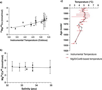
After the elimination threshold was applied (Supplementary Table S2), 43 measurements remained for analysis. The 24Mg/48Ca ranges from 1.72 to 9.01 mmol/mol (Supplementary Table S3). The P value for the linear regression model of isotope ratios was <0.05, representing a significant relationship between bottom-water temperature and Mg/Ca ratio (Fig. 2a). For both linear and nonlinear (exponential) models, the R-squared values were >0.7, indicating a significant correlation between temperature and the Mg/Ca ratio (Supplementary Table S4). The exponential equation was chosen, because it yielded a higher R-squared (R 2 = 0.76) than that of the linear model (R 2 = 0.74).
Best-fit curve for the multi-element solution (MeRC)-corrected 24Mg/48Ca data against (a) instrumental temperature and (b) instrumental salinity, respectively. Error bars represent the standard deviation of replicate measurements. In c, we plot instrumental temperature and reconstructed temperature from core CR02-23 based on MeRC-corrected 24Mg/48Ca data best fit. Error bars represent standard deviation from replication measurement (temperature, x-axis) and error from 210Pb CRS-model (year, y-axis).

Figure 2 Long description
The image A showing a scatter plot with error bars and a fitted curve. Vertical axis label: 24Mg/48Ca (mmol/mol). Range: 0 to 8. Horizontal axis label: Instrumental Temperature (Celcius). Range: 3.0 to 5.5. Horizontal axis tick labels: 3.0, 3.5, 4.0, 4.5, 5.0, 5.5. Vertical axis tick labels: 0, 2, 4, 6, 8. Plotted points appear between about 3.1 and 5.2 on the horizontal axis and about 1.8 and 5.0 on the vertical axis. Error bars are shown on multiple points. The fitted curve rises from lower values near the 3.0 to 3.5 temperature range to higher values near the 5.0 to 5.5 temperature range. The image B showing a scatter plot with error bars. Vertical axis label: Mg/Ca48 (mmol/mol). Range: 0 to 8. Horizontal axis label: Salinity (psu). Range: 32 to 35. Horizontal axis tick labels: 32, 33, 34, 35. Vertical axis tick labels: 0, 2, 4, 6, 8. Plotted points appear near 32.2 to 35.0 on the horizontal axis and near 3.0 to 4.2 on the vertical axis. Error bars are shown on the points. The points form a near-horizontal band across the salinity range, with similar Mg/Ca48 values at salinity 32, 33, 34 and 35. The image C showing a line plot with markers and horizontal error bars, with two series and a legend. Top axis label: Temperature (C). Range: 2 to 8. Top axis tick labels: 2, 3, 4, 5, 6, 7, 8. Vertical axis label: Age model. Range: 1920 to 2000. Vertical axis tick labels: 1920, 1930, 1940, 1950, 1960, 1970, 1980, 1990, 2000. Legend text: Instrumental temperature; 24Mg/48Ca-based temperature. One series is drawn as a connected line with markers, with points spanning from about 1930 to about 1995 and temperatures around 3.5 to 5.5. A second series is shown with markers and horizontal error bars across multiple ages, with temperatures around 3.5 to 6.0. The two series overlap closely at several ages around the mid-range temperatures and show wider separation at some ages where one series is nearer about 5.5 to 6.0 while the other is nearer about 4.0 to 4.5.
Salinity effect and contamination
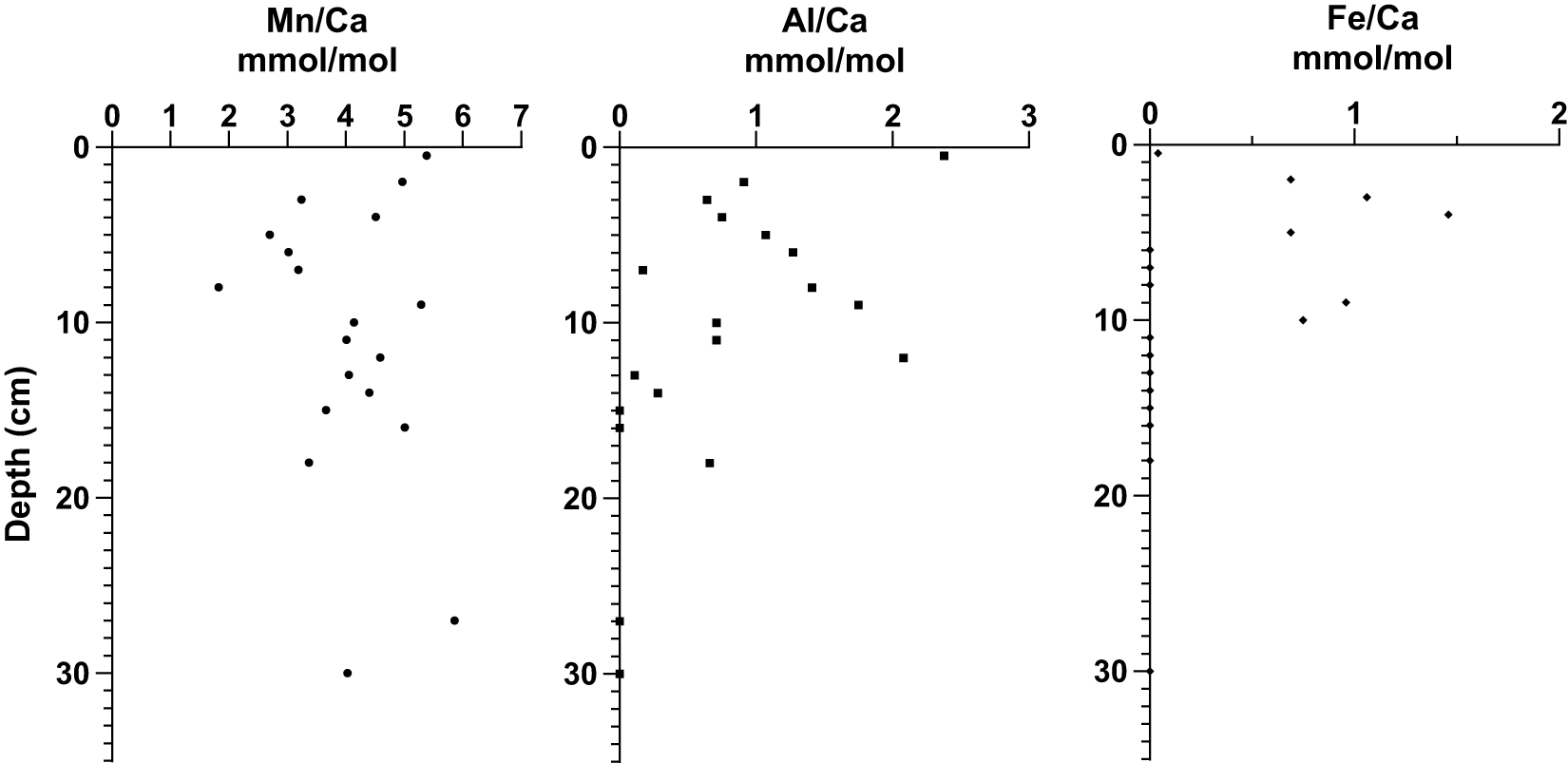
No statistically significant relationship was observed between salinity and Mg/Ca (P value > 0.05, R 2 < 0.02; Fig. 2b; Supplementary Table S5). However, the lack of correlation could result from the small sample size (n = 8) and the narrow salinity range (32.34 to 34.94 psu). No significant correlation was observed between Mn/Ca or Fe/Ca with Mg/Ca (Fig. 3). A low but significant correlation was observed between Al/Ca and Mg/Ca, suggesting minimal contamination.
Ratio of contaminant (Mn, Al, and Fe) on Ca down-core of CR02-23.

Figure 3 Long description
Three scatter plots are arranged left to right. Left scatter plot title: Mn slash Ca. Unit: millimole over mole. The horizontal axis shows Mn slash Ca from 0 to 7. The vertical axis label is Depth (centimeter), with labeled ticks at 0, 10, 20 and 30. Points appear across depths from near 0 to about 30. Mn slash Ca values appear mostly between about 2 and 6, with one point near depth about 30 at around 4 and one point near depth about 27 at around 6. Middle scatter plot title: Al slash Ca. Unit: millimole over mole. The horizontal axis shows Al slash Ca from 0 to 3. The vertical axis uses the same Depth (centimeter) scale with labeled ticks at 0, 10, 20 and 30. Points appear across depths from near 0 to about 30. Al slash Ca values appear mostly between about 0 and 2, with one point near the top close to 3 and several points near 0 at depths around the mid to lower part of the axis. Right scatter plot title: Fe slash Ca. Unit: millimole over mole. The horizontal axis shows Fe slash Ca from 0 to 2. The vertical axis uses the same Depth (centimeter) scale with labeled ticks at 0, 10, 20 and 30. Points are concentrated in the upper part of the depth range, mostly above 15. Fe slash Ca values appear mostly between about 0.5 and 1.5, with one point close to 0 near the top of the axis.
MD99-2220
A total of 286 foraminiferal samples were analysed. After the elimination threshold was applied, 100 measurements remained for data analysis.
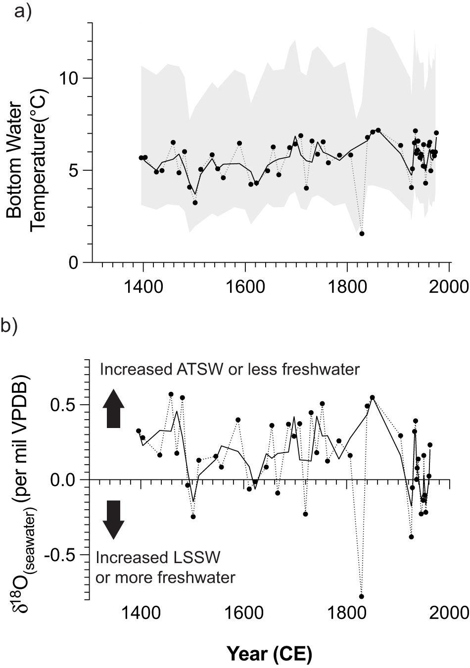
The average Mg/Ca ratio in MD99-2220 across depths 0 cm to 76 cm ranged from 1.14 to 9.16 mmol/mol. Reconstruction yielded bottom-water temperatures of 1.58–7.18°C (Fig. 4a). We observed a stepwise increase in temperature from ∼1396 to 1905 CE, followed by a decrease from ∼1905 CE onwards with large fluctuations in the twentieth century. The seawater isotope signal declined from the base of the record until ∼1500 CE, then increased stepwise until ∼1800 CE, after which a sharp decrease was recorded (Fig. 4b). Because of the relatively high standard deviation of our measurements, we remained cautious when discussing small-amplitude variations in our record.
(a) Bottom-water temperature reconstruction and (b) seawater oxygen isotope reconstruction of the St. Lawrence Estuary from 1396 to 1975 CE. The thick lines correspond to a three-point moving average. Temperature uncertainty was set at 95% of the confidence interval of the equation fit of the three-point moving average, excluding the outlier at 1829 CE. ATSW, Atlantic Temperate Slope Water; LSSW: Labrador Subarctic Slope Water.

Figure 4 Long description
The image A showing a line graph. Vertical axis label: Bottom Water Temperature left parenthesis degree C right parenthesis. Vertical axis range: 0 to 10. Horizontal axis tick labels: 1400, 1600, 1800, 2000. A series of circular markers connected by a dotted line spans from near 1400 to near 2000. A second line runs through the markers. Visible marker values include points near: 1400 about 5.5; mid 1400s about 6.5; around 1500 about 3.5; around 1600 about 4.5 to 5.5; around 1700 about 6.0 to 6.5; around 1800 about 5.5 to 6.5; one low point near the early 1800s about 1.5; mid to late 1800s about 6.5 to 7.0; early 1900s about 6.0; mid 1900s about 4.5; late 1900s multiple points about 5.0 to 7.0. The image B showing a line graph. Text above the plot: Increased ATSW or less freshwater. Text below the plot: Increased LSSW or more freshwater. Vertical axis label: delta 18 O left parenthesis seawater right parenthesis left parenthesis per mil VPDB right parenthesis. Vertical axis range: negative 0.5 to positive 0.5. Horizontal axis label: Year left parenthesis CE right parenthesis. Horizontal axis tick labels: 1400, 1600, 1800, 2000. A horizontal reference line is drawn at 0.0. A series of circular markers connected by a dotted line spans from near 1400 to near 2000. A second line runs through the markers. Visible marker values include points near: early 1400s about 0.3; mid 1400s about 0.2; late 1400s about 0.6; around 1500 about negative 0.2; around 1600 about 0.1 to 0.3; around 1700 about 0.2 to 0.5; one low point near the early 1800s about negative 0.7; mid 1800s about 0.5 to 0.6; early 1900s about 0.3; mid 1900s about negative 0.4; late 1900s multiple points about negative 0.2 to 0.3.
Discussion
Calibration of Mg/Ca versus temperature in the St. Lawrence Estuary
Comparisons of calibrations
We compared the CR02-23 Mg/Ca ratio with previously established calibrations for temperature estimates from Mg/Ca, thereby testing the applicability of published equations (Lear et al., Reference Lear, Rosenthal and Slowey2002; Weldeab et al., Reference Weldeab, Arce and Kasten2016) for G. auriculata at our study location. The temperature reconstructions using published equations yield a wide range of values (−1°C to 28°C), well outside the study environment’s range (3°C to 6°C). This highlights the need for a regional calibration curve using Globobulimina auriculata.
Calibration equation for Globobulimina auriculata in the lower St. Lawrence Estuary
The calibration equation was established as the best-fit exponential equation from 24Mg/48Ca data after MeRC correction and instrumental temperature from the St. Lawrence bottom water (Thibodeau et al., Reference Thibodeau, Not, Zhu, Schmittner, Noone, Tabor, Zhang and Liu2018):
 \begin{equation}{\text{Mg}}/{\text{Ca }}\left( {{\text{mmol}}/{\text{mol}}} \right) = 0.6341{e^{\left( {0.3740T} \right)}}\end{equation}
where T represents water temperature in Celsius.
This equation yielded a range of bottom-water temperatures of 3.0°C to 5.5°C, with an R-square of 0.76 between instrumental and estimated values. It is important to note that this calibration used Mg/Ca values from the sediment core and instrumental temperature records on a calendar-year scale. Therefore, the correlation may be affected by uncertainty in the core chronology. Moreover, because we used the local temperature gradient over time, the calibration covers only a 3°C temperature range. While this calibration can provide a fine-scale reconstruction, the narrow temperature range may have amplified uncertainty in the relationship between the actual and reconstructed data, resulting in a relatively low coefficient of correlation. Finally, assuming that carbonate ion concentration mainly affects the Mg/Ca ratio at bottom-water temperatures <3°C (Elderfield et al., Reference Elderfield, Yu, Anand, Kiefer and Nyland2006), we did not account for the effect of carbonate ion, which may be an additional caveat. Regardless of these potential limitations, the calibration equation tailored to G. auriculata in the lower St. Lawrence Estuary appears robust for regional reconstructions of temperature through time. However, it is important to note that the most recent part of the record includes data that are outside our calibration range, which may explain the higher variability observed, notably in the most recent part of the cores where temperatures are expected to be warmer.
LIA temperature reconstruction
Changes in bottom-water temperature reconstructed from our Mg/Ca data followed a pattern similar to our expectation based on literature, namely a cooling at the beginning of the LIA following by a gradual warming throughout the LIA (e.g., Keigwin, Reference Keigwin1996; Thibodeau et al., Reference Thibodeau, Not, Zhu, Schmittner, Noone, Tabor, Zhang and Liu2018; Forman et al., Reference Forman, Baldini, Jamieson, Lechleitner, Walczak, Nita and Smith2025; Keigwin et al., Reference Keigwin, Petrie and Boyle2025; Fig. 4a). Our calculated δ18Oseawater was characterized by a pattern similar to that of the temperature (Fig. 4b), supporting previous interpretation suggesting that the dominant factor controlling temperature changes is likely related to the mixing proportions of parent water masses in the bottom water of the lower St. Lawrence Estuary.
A nonparametric Mann-Kendall trend test was applied to identify significant trends. A positive trend characterized the ∼1490 to ∼1850 CE interval for both δ18Oseawater and temperature (Supplementary Table S6). Transitions were thus identified at 1490 and 1850 CE, yielding three time intervals in the study sequence (Fig. 5), which are discussed hereafter with reference to potential drivers of change in the dynamics of western North Atlantic circulation during the LIA. This segmentation is aligned with previous studies suggesting the onset of the LIA in this region to be around 1500 CE (e.g., Keigwin et al., Reference Keigwin, Petrie and Boyle2025).
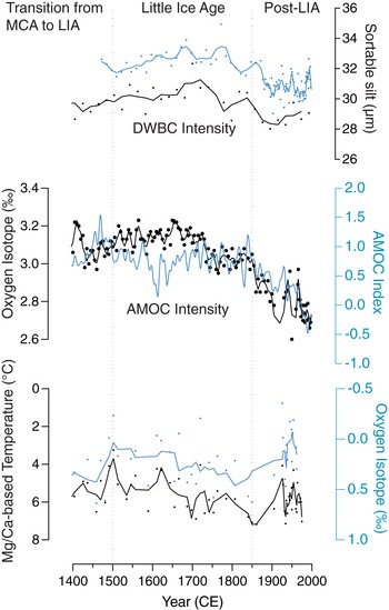
Comparison of selected Little Ice Age (LIA) records with our result. Top, Sortable silt in core KNR-178-48JPC (in blue) and KNR-178-56JPC (in black), which is used as a proxy of flow speed of the deep western boundary current (DWBC) (Thornalley et al., Reference Thornalley, Oppo, Ortega, Robson, Brierley, Davis and Hall2018). Middle, Atlantic Meridional Overturning Circulation (AMOC) index in blue (Rahmstorf et al., Reference Rahmstorf, Box, Feulner, Mann, Robinson, Rutherford and Schaffernicht2015) and δ18O of Globobulimina auriculata in core MD99-2220 (Thibodeau et al., Reference Thibodeau, de Vernal, Hillaire-Marcel and Mucci2010, Reference Thornalley, Oppo, Ortega, Robson, Brierley, Davis and Hall2018). Bottom, Bottom-water reconstruction for Mg/Ca of G. auriculata from core MD99-2220 (this study) in black and reconstructed seawater δ18O (this study) in blue. The black vertical dashed lines indicate the suggested separation between different time intervals. MCA.

Figure 5 Long description
Transition from MCA to LIA Little Ice Age Post-LIA Three stacked line graphs share the x-axis label Year (CE), with tick labels at 1400, 1500, 1600, 1700, 1800, 1900 and 2000. Two vertical dashed lines align with 1500 and 1850. Top graph: The right y-axis is labeled Sortable silt (micrometer), with tick labels 26, 28, 30, 32, 34 and 36. Two plotted series are shown as a blue line with blue dots and a black line with black dots. The blue series is near 32 around 1400, rises to about 33 to 34 between about 1600 and 1750, then drops to about 30 to 31 after about 1850, with dense fluctuations between about 1900 and 2000. The black series is near 29 around 1400, rises to about 31 by about 1700, then declines to about 28 to 29 after about 1850 and ends near about 29 to 30 by about 2000. Middle graph: The left y-axis is labeled Oxygen Isotope (per mil), with tick labels 2.6, 2.8, 3.0, 3.2 and 3.4. The right y-axis is labeled AMOC Index, with tick labels minus 1.0, minus 0.5, 0.0, 0.5, 1.0, 1.5 and 2.0. A black line with black dots varies around 3.0 to 3.2 from about 1400 to about 1750, then trends downward after about 1800, reaching about 2.7 to 2.9 between about 1900 and 2000, with a low dot near about 2.6 in the late part of the record. A blue line varies around about 0.5 to 1.2 before about 1800, then declines after about 1850, reaching near 0.0 and below, with values near about minus 0.5 close to the end. Bottom graph: The left y-axis is labeled Mg/Ca-based Temperature (degree C), with tick labels 0, 2, 4, 6 and 8. The right y-axis is labeled Oxygen Isotope (per mil), with tick labels minus 1.0, minus 0.5, 0.0 and 0.5. A black line with black dots is mostly between about 5 and 7 from about 1400 to about 1850, with a dip toward about 7 near the 1800s, then shows clustered points and short segments between about 5 and 7 after about 1900. A blue line with blue dots is around about 0.3 to 0.5 from about 1400 to about 1700, shifts toward about 0.2 to 0.3 by about 1800, then rises after about 1850 toward about 0.0 near the late 1900s, with a short upward spike near the end.
Transition from MCA to LIA (pre-1500 CE)
This time interval was characterized by a relatively constant signal, followed by a relatively sharp decrease in both temperature and seawater δ18O in the latter half of the fifteenth century, suggesting increased influence of Labrador-derived water at our site. This cooling is synchronous with an increase in the size of sortable silt from the southeast Grand Banks, suggesting an increase in Labrador Current flow speed since ∼1450 CE (Rashid et al., Reference Rashid, Zhang, Piper, Patro and Xu2023), before the rise in the contribution of LSSW as reconstructed herein. This may have been caused by an increase in freshwater transport into the Labrador Sea slope waters as suggested by modern observational data (Lazier and Wright, Reference Lazier and Wright1993). Increased freshwater release in the Labrador Sea has been reconstructed for the LIA, which may originate from meltwater produced during the warm MCA (Moffa-Sánchez et al., Reference Moffa-Sánchez, Hall, Barker, Thornalley and Yashayaev2014; Alonso-Garcia et al., Reference Alonso-Garcia, Kleiven, McManus, Moffa-Sanchez, Broecker and Flower2017; Lapointe and Bradley, Reference Lapointe and Bradley2021). This freshwater discharge has been observed from TEX86-T and higher presence of polar waters at Eirik Drift (Rashid et al., Reference Rashid, Zhang, Piper, Patro and Xu2023). These pieces of evidence also aligns with relatively cool condition in the Sargasso Sea (Keigwin, Reference Keigwin1996) and relatively low δ18O, indicating fresh and cold conditions in the Jordan Basin (Keigwin et al., Reference Keigwin, Petrie and Boyle2025). This explains the cooling observed from ∼1470 CE in our core (Fig. 4a) and the higher presence of stronger Labrador Sea current–derived waters (Fig. 4b). This is also consistent with a weakened Gulf Stream (Rahmstorf et al., Reference Rahmstorf, Box, Feulner, Mann, Robinson, Rutherford and Schaffernicht2015; Caesar et al., Reference Caesar, Rahmstorf, Robinson, Feulner and Saba2018), and reduced northward heat transport (Lund et al., Reference Lund, Lynch-Stieglitz and Curry2006) lessening the relative contribution of the ATSW as estimated from our record (Fig. 4).
The LIA (∼1500 to 1850 CE)
In the study region, the LIA was characterized by a significant increasing trend of oxygen isotope signature and bottom-water temperature (Supplementary Table S6). The coldest and freshest subsurface water in the Labrador Sea was recorded right at the beginning of the sixteenth century, as indicated by our Mg/Ca ratios, which is consistent with δ18O values in Neogloboquadrina pachyderma (Moffa-Sánchez et al., Reference Moffa-Sánchez, Hall, Barker, Thornalley and Yashayaev2014). Gradually during the LIA, more saline waters were observed until around 1800 CE (Lund et al., Reference Lund, Lynch-Stieglitz and Curry2006) and can be attributed to drier conditions in the West Atlantic (Saenger et al., Reference Saenger, Came, Oppo, Keigwin and Cohen2011). The increased salinity of the Gulf Stream, resulting in a higher oxygen isotope composition of the ATSW, might have contributed to the rise in δ18Oseawater in our reconstruction (Fig. 4b).
The end of LIA (∼1810–1850 CE) coincides with the early stage of the industrial era (∼1830 CE onward), during which air temperature and sea-surface temperature recorded <0.2°C and <0.5°C increases, respectively (Abram et al., Reference Abram, McGregor, Tierney, Evans, McKay and Kaufman2016). However, climate-related warming cannot account for the ∼2°C increase observed in bottom-water temperature (Fig. 5). Therefore, we hypothesize that the regional warming was mainly caused by the enhanced contribution of ATSW relative to LSSW. The timing of the peak matched the end of the large-scale ice-rafting events in ∼1800 CE (Alonso-Garcia et al., Reference Alonso-Garcia, Kleiven, McManus, Moffa-Sanchez, Broecker and Flower2017) and the end of the series of volcanic eruptions (∼1835 CE) (Brönnimann et al., Reference Brönnimann, Franke, Nussbaumer, Zumbühl, Steiner, Trachsel and Hegerl2019). A decrease in the deep western boundary current (DWBC) was also inferred from sortable silt (Thornalley et al., Reference Thornalley, Oppo, Ortega, Robson, Brierley, Davis and Hall2018), which may reduce the amount of δ18O-depleted water reaching this site and thus explains the maximum oxygen isotopic signal observed during this interval. This is also consistent with other studies suggesting a gradual northward displacement of the Gulf Stream in the later stage of the LIA (Forman et al., Reference Forman, Baldini, Jamieson, Lechleitner, Walczak, Nita and Smith2025).
Post-LIA (post-1850 CE)
This beginning of this interval has lower resolution, mostly due to contaminated samples, and thus the comparison with other records is not straightforward. Moreover, we observed very high variability, especially in the twentieth century. The start of this interval was marked by an important cooling of approximately 3°C of bottom-water temperature between ∼1850 CE and ∼1925 CE. While this cooling seems to align with a resurgence of LSSW at our site and a strengthening of the AMOC (Fig. 5), it is only recorded in two samples and thus should be interpreted with caution. Moreover, this cooling is immediately followed by a 3°C warming between ∼1925 CE and ∼1934 CE. The following two decades are then characterised by a cooling of about 2.5°C, followed by a similar warming of >2°C in the second half of the twentieth century (∼1954 CE to the end of our record). Interestingly, the observed cooling at the beginning of this period coincides with a short-lived peak in hematite-stained grain abundance in the Labrador Sea, indicating a sudden and significant increase in Arctic sea-ice export through the Eastern Greenland Current (Alonso-Garcia et al., Reference Alonso-Garcia, Kleiven, McManus, Moffa-Sanchez, Broecker and Flower2017). Therefore, the drop in δ18Oseawater may be caused by an increase in Labrador-derived water, but also by the freshening of this endmember. The latter could also explain why this cooling seems at odds with other interpretations of regional δ18O records that suggested a warming from the beginning of the twentieth century (Thibodeau et al., Reference Thibodeau, Not, Zhu, Schmittner, Noone, Tabor, Zhang and Liu2018; Keigwin et al., Reference Keigwin, Petrie and Boyle2025). However, a transient cooling of about 2°C was also observed in the Jordan Basin deep water, with coldest conditions around 1920 CE (Keigwin et al., Reference Keigwin, Petrie and Boyle2025). Moreover, while the Gulf Stream was strengthening as well after the end of the LIA, its δ18Oseawater also dropped by ∼0.3‰ (Lund et al., Reference Lund, Lynch-Stieglitz and Curry2006). Therefore, evidence of lower δ18Oseawater values in both endmembers composing the Laurentian bottom water suggests that the isotopic signal may have been primarily controlled by changes in the isotopic composition of these water masses due to freshwater input following the LIA rather than temperature as suggested by previous studies. In the second half of the twentieth century, we reconstructed a 2°C warming, consistent with multiple observations in the region, and that was attributed to an increased influence of Atlantic-derived water over the Canadian shelf, which is also present in our reconstruction of seawater δ18O (Keigwin et al., Reference Keigwin, Sachs and Rosenthal2003, Reference Keigwin, Petrie and Boyle2025; Gilbert et al., Reference Gilbert, Sundby, Gobeil, Mucci and Tremblay2005; Thibodeau et al., Reference Thibodeau, de Vernal and Mucci2006, Reference Thibodeau, de Vernal, Hillaire-Marcel and Mucci2010, Reference Thibodeau, de Vernal and Limoges2013, Reference Thornalley, Oppo, Ortega, Robson, Brierley, Davis and Hall2018; Genovesi et al., Reference Genovesi, de Vernal, Thibodeau, Hillaire-Marcel, Mucci and Gilbert2011).
Conclusion
In this paper, we used single foraminifer ICP-MS to establish an exponential Mg/Ca–temperature calibration curve for Globobulimina auriculata at the lower St. Lawrence Estuary:  ${\text{Mg}}/{\text{Ca }}\left( {{\text{mmol}}/{\text{mol}}} \right) = 0.6341{e^{\left( {0.3740T} \right)}}$. This bottom-water temperature reconstruction curve applies to a temperature range of 3.0–5.5°C. Despite its narrow temperature range, it provides a species- and region-specific curve for relatively accurate temperature reconstruction in future studies. Using the newly established calibration curve and Mg/Ca data from the MD99-2220 core, we reconstructed the bottom-water temperature in the lower St. Lawrence Estuary during the LIA. Constrained by δ18Ocalcite data, we calculated the change in δ18Oseawater and used it as a proxy for the change in the contribution of the parent water mass. Our results, taken together with previous evidence, indicate that the transition from MCA to LIA was characterized by a sharp decrease in temperature and oxygen isotope values, likely due to increased Labrador Sea–derived water. During the LIA, there was an increasing trend in oxygen isotope signal and bottom-water temperature, with a shift from LSSW to ATSW dominance. The post-LIA period began with a sharp decrease in bottom-water temperature, followed by a significant warming trend in the late twentieth century, attributed to an increased influence of Atlantic-derived water masses over the Canadian continental shelf.
Supplementary material
The supplementary material for this article can be found at https://doi.org/10.1017/qua.2026.10100
Acknowledgments
The authors are grateful for the technical support provided by Cho On Thomas Tang from the Chinese University of Hong Kong for his help troubleshooting the Agilent 7900 ICP-MS.
Data Availability Statement
Data produced for this paper are available at https://doi.org/10.48668/HLKYYR.
Funding
This study was funded through the General Research Fund from the Research Grant Council of Hong Kong (#17301320) awarded to Benoit Thibodeau. The sampling and study of marine sediment cores MD99-2220 and CR02-23 were enabled thanks to the support of the Natural Science and Engineering Research Council (NSERC) of Canada and the Fonds de Recherche du Québec–Nature et Technologie (FRQNT).
Author Contributions
WCRC: Methodology, formal analysis, investigation, data curation, writing—original draft, review, and editing, visualization. AdV: Resources, writing—review and editing. TA: Resources, writing—review and editing. BT: Conceptualization, resources, data curation, visualization, supervision, project administration, funding acquisition, writing—review and editing.
Declaration of competing interests
The authors declare that they have no known competing financial interests or personal relationships that could have appeared to influence the work reported in this paper.



 Open access

