


1. Introduction
Shock tubes are devices used to generate shockwaves in a safe and reproducible manner in laboratory confinement. A simple shock tube has a high-pressure chamber (known as the driver section) and a low-pressure chamber (known as the driven section) separated by a diaphragm. The diaphragm rupture leads to a shockwave formation, which propagates down the driven section of the shock tube (Bradley Reference Bradley1962; Gaydon & Hurle Reference Gaydon and Hurle1963). Shock tubes are commonplace in research laboratories to facilitate chemical kinetic studies, supersonic and hypersonic investigations. Although seemingly simple devices, shock tubes are a subject of intense scrutiny with several unanswered questions. Shock formation and attenuation in shock tubes have been areas of long-standing research. Over the years, there have been reports that address these aspects, albeit at low initial pressures in the driven section and using limited experiments. Emerging transdisciplinary applications of shockwaves have been demonstrated at initial ambient conditions at miniature scales. Shockwave-assisted applications using miniature shock tubes in needleless drug delivery (Janardhanraj et al. Reference Janardhanraj, Akshay, Jagadeesh and Dipshikha2017), bacterial transformation (Akshay et al. Reference Akshay, Janardhanraj, Jagadeesh and Dipshikha2017) and suppression of cavity noise (Ramachandran et al. Reference Ramachandran, Raman, Janardhanraj and Jagadeesh2010) typifies the growing interest in this area. Miniature shock tubes driven by lasers have been reported for use in hydrodynamic studies and spectroscopy studies (Zvorykin & Lebo Reference Zvorykin and Lebo2000; Busquet et al. Reference Busquet, Barroso, Melse and Bauduin2010). High repetition miniature shock tubes have been developed using high-speed pneumatic valves for high-pressure and high-temperature reacting systems (Tranter & Lynch Reference Tranter and Lynch2013; Lynch et al. Reference Lynch, Troy, Ahmed and Tranter2015). Extensive experiments and exhaustive analysis are essential to provide insights into the shockwave formation, propagation and attenuation dynamics in miniature shock tubes operated at initial ambient conditions for further development of shockwave-based applications.
A brief review of the studies on the shockwave formation and attenuation is useful. Glass & Martin (Reference Glass and Martin1955) were among the first to report that there are two main reasons for attenuation in a shock tube, namely, the shock formation process and the effects due to the shock tube walls. But there was a lack of experimental data to validate this model for different operating conditions in shock tubes. White (Reference White1958) proposed a model to account for the finite time taken by the diaphragm to rupture in large diameter shock tubes operated at high diaphragm pressure ratios. He experimentally showed that the shockwave velocity could be higher than the values predicted by the one-dimensional inviscid shock tube theory. Emrich & Curtis (Reference Emrich and Curtis1953) predicted that stronger shockwaves attenuate faster than weaker shockwaves, and the attenuation per unit length is almost independent of distance. Mirels (Reference Mirels1963, Reference Mirels1964) and Emrich & Wheeler Jr (Reference Emrich and Wheeler1958) helped understand the wall effects in shock tube flow by accounting for the boundary layer development behind the moving shock front. Ikui, Matsuo & Nagai (Reference Ikui, Matsuo and Nagai1969) provided an improved multistage approach to White's model for the shock formation process. They also proposed a relation between shock formation distance( $x_f$) and hydraulic diameter ( $D$) of the shock tube as $x_f \propto D^{0.88}$ (Ikui & Matsuo Reference Ikui and Matsuo1969). Rothkopf & Low (Reference Rothkopf and Low1974) described the diaphragm opening process for different materials used as diaphragms. They also clearly defined the shock formation distance as the distance from the diaphragm location where the shock speed reaches its maximum value. Rothkopf & Low (Reference Rothkopf and Low1976) presented a qualitative description of the diaphragm opening process in shock tubes, which is an important parameter that decides the shock formation distance. Their experimental results showed good agreement with the relation present by Drewry & Walenta (Reference Drewry and Walenta1965) for the diaphragm opening time ( $t_{op}$) given by
 \begin{equation} t_{op} = K\sqrt{\frac{\rho\cdot b\cdot th}{P_4}}, \end{equation}
where  $\rho$ is the density of the material, $b$ is the length of the petal base, $th$ is the petal thickness, $P_4$ is the bursting pressure and $K$ is taken as 0.93. Simpson, Chandler & Bridgman (Reference Simpson, Chandler and Bridgman1967) represented the shock formation distance as $x_f=K_1\cdot V_{Smax}\cdot t_{op}$, where $V_{Smax}$ is the maximum shock velocity, $t_{op}$ is the opening time of the diaphragm and $K_1$ is the constant of proportionality. Rothkopf & Low (Reference Rothkopf and Low1976) reported that the value of $K_1$ mostly lies between 1 and 3, and sometimes greater than 3. Ikui, Matsuo & Yamamoto (Reference Ikui, Matsuo and Yamamoto1979) observed that the shockwave becomes planar at a distance, which is approximately a fifth of the shock formation distance.
Studies in a microchannel with a hydraulic diameter of 34  $\mathrm {\mu }$m revealed that shockwave propagation at micro-scales exhibits a behaviour similar to that observed in larger-scale facilities operated at low initial pressures (Mirshekari & Brouillette Reference Mirshekari and Brouillette2012). Mirshekari & Brouillette (Reference Mirshekari and Brouillette2009) performed experiments in a 5.3 mm diameter shock tube at low initial driven section pressures (typically $P_1 < 100$ mbar) and showed good qualitative agreement with a flow model based on a scaling parameter $Scl=Re'D/4L$, where $Re'$ is the characteristic Reynolds number based on the driven gas, $D$ is the hydraulic diameter of the tube and $L$ is the characteristic length. Arun & Kim (Reference Arun and Kim2012), Arun, Kim & Setoguchi (Reference Arun, Kim and Setoguchi2012), Arun & Kim (Reference Arun and Kim2013) and Arun, Kim & Setoguchi (Reference Arun, Kim and Setoguchi2013, Reference Arun, Kim and Setoguchi2014) presented a series of numerical reports on the shock formation process in micro-shock tubes due to the gradual rupture of the diaphragm when operated at very low initial pressures in the driven section. They reported that the shockwave attenuation is significantly higher in micro-shock tubes as compared to macro-scale shock tubes. Sun, Ogawa & Takayama (Reference Sun, Ogawa and Takayama2001) reported that viscous effects in channels the height of which is below 4 mm become noticeable even at atmospheric pressure. Park, Kim & Kim (Reference Park, Kim and Kim2012) reported that at the same initial conditions, the shockwave attenuation in a 3 mm shock tube is more significant than in a 6 mm shock tube. Zeitoun & Burtschell (Reference Zeitoun and Burtschell2006) used two-dimensional (2-D) Navier–Stokes computations with slip velocity and temperature jump boundary conditions to predict flow in micro-scales. Numerical studies by Ngomo et al. (Reference Ngomo, Chaudhuri, Chinnayya and Hadjadj2010) show that the flow in microchannels shows a transition from an adiabatic regime to an isothermal regime. A one-dimensional numerical model to predict micro-scale shock tube flow was presented by Mirshekari & Brouillette (Reference Mirshekari and Brouillette2009) by integrating the three-dimensional diffusion effects as sources of mass, momentum and energy in the axial conservation equations. Giordano et al. (Reference Giordano, Parisse, Biamino, Devesvre and Perrier2010) studied the transmission of weak shock waves through 1.02 and 0.48 mm miniature channels. Mirshekari et al. (Reference Mirshekari, Brouillette, Giordano, Hebert, Parisse and Perrier2013) later complemented their experimental results with a Navier–Stokes model, which assumes a no-slip isothermal wall boundary condition. Recently, pressure measurements and particle tracking velocimetry were made in a 1 mm square shock tube operating at diaphragm pressure ratios of 5 and 10 (Zhang et al. Reference Zhang, Lee, Hashimoto, Setoguchi and Kim2016).
The present study highlights the shock attenuation phenomena in miniature shock tubes for operating conditions similar to the practical scenario used in the shockwave-based applications. The most commonly used diameters of shock tubes for transdisciplinary applications are in the range of 10 mm or lower. Also, the driven section of the shock tube is generally kept at ambient conditions. Therefore, experiments are performed in a 2, 6 and 10 mm shock tube with a square cross-section in a unique table-top shock tube facility in the present work. A square cross-section is chosen to facilitate visualization studies of the driven section of the shock tube. For the first time, the shock tube's entire driven section is visualized to study the shockwave formation and attenuation. Nitrogen and helium are used as driver gases, and the diaphragm pressure ratio is also varied. The obtained results from the experiments are compared with analytical and computational models reported in the literature. The wave phenomena that occur immediately after the diaphragm rupture in the driven section of the shock tube are discussed in detail. The formation of the Mach stem and triple point due to the diaphragm's finite opening time and the evolution of a planar shock front are presented. Correlations are developed based on the experimental and numerical findings to predict the shock Mach number's variation along the entire length of the driven section. These correlations perform satisfactorily for the present experimental findings and data reported in the open literature.
2. Experimental methodology
2.1. Shock tube facility
The present study uses a unique table-top shock tube designed and built in-house at the Laboratory for Hypersonic and Shockwave Research, Indian Institute of Science, Bengaluru, India. This particular experimental set-up, which has a quick-changing diaphragm mechanism, is used for pressure measurements and visualization studies in miniature shock tubes. The experimental set-up is similar to the one described in a previous study (Janardhanraj & Jagadeesh Reference Janardhanraj and Jagadeesh2016) with additional features. The shock tube's internal dimension can be changed to either a 2, 6 or 10 mm square cross-section. The length of the driver section is 100 mm, while the driven section has a length of 339 mm. Three separate driver sections of 2, 6 and 10 mm square internal cross-section of length 100 mm are fabricated (see figure 1a). There is also a diaphragm puncture mechanism incorporated in the shock tube (see figure 1b). A long needle is connected to the driver section's rear end to puncture the diaphragm (see figure 1c). A knob moves the needle in the forward direction (a total distance of about 5 mm) when rotated. This mechanism can be used interchangeably in the three different driver sections. Two optical quality BK-7 glass slabs form the walls of the driven section of the shock tube (see figure 1d). Metal channels restrict the motion of the BK-7 glass in the lateral direction. The driven section arrangement encloses either a 2 mm × 2 mm, 6 mm × 6 mm or 10 mm × 10 mm cross-section (see figure 1f). A separate fixture houses the entire assembly of the driven section. Adjusting screws on top of the fixture holds the driven section in place firmly (see figure 1e). The fixture's metal frame obstructs a small region covering a distance of 4 mm immediately after the diaphragm location and another region covering a distance of 35 mm towards the end of the driven section. The total unobstructed length of the driven section that can be viewed from a direction perpendicular to the shock tube axis is 300 mm. During pressure measurements, the BK-7 glasses are replaced by a composite plate that houses the pressure sensors, the details of which are given in the subsequent section. All components are made of stainless steel (SS-304 grade). The tolerance of the machined components is  ${\pm }0.02$ mm.
(a) Computer-aided design models showing the driver sections of the three shock tubes. (b) Diaphragm puncture mechanism used in the driver section. (c) Assembly of the diaphragm puncture mechanism in the driver section. (d) Exploded view showing the assembly of the BK-7 glass slabs. (e) Assembly of the driven section of the shock tube. (f) Cross-section showing the driven section of the three shock tubes.

2.2. Measurement of pressure
The pressure of the shock tube's driver gas is measured using a digital pressure gauge (SW2000 series, Barksdale Control Products, Germany) with an operating range of 0–50.0 bar and a least count of 0.1 bar. The pressure histories inside the driven section of the shock tube are obtained using the ultra-miniature pressure transducers (LQ-062 series, Kulite Semiconductor Products Inc., USA). The sensor's natural frequency is 300 kHz, and the rise time is typically 1.3  $\mathrm {\mu }$s. The sensing region of the transducer has a diameter of 1.6 mm. These sensors are mounted on a composite plate arrangement that ensures that the sensing surface is flush with the shock tube walls. The sensors were installed according to the manufacturer's instructions. Figure 2 shows the top view and the cross-sectional view of the composite plate. An acrylic plate and a stainless-steel plate are sandwiched together. The acrylic plate is used near the sensor to avoid any electrically conducting material. The inside of the acrylic plate is modified to expose only the sensing surface of the pressure sensor. The leads of the sensor are drawn out through a small hole made in the stainless-steel plate. Suitable backing is given to the sensor to ensure the sensing surface remains flush to the plate surface. A screw fastens the acrylic and the stainless-steel plate together. Two miniature pressure sensors are mounted in the shock tube's driven section at a distance of 291 mm (sensor 1) and 331 mm (sensor 2) from the diaphragm location. A signal conditioning rack (DEWETRON GmbH, Germany) is used for data acquisition from the miniature transducers. The signals are obtained without any amplification from the signal conditioner. A 300 kHz filter is used to cut off the unwanted frequencies embedded in the signal.
A 2-D drawing showing the top view and cross-sectional view of the composite plate that accommodates the ultra-thin miniature pressure transducers.

2.3. Shadowgraphy
The shockwave propagation in the driven section of the shock tube is captured using a high-speed shadowgraphy technique (Settles Reference Settles2001). The set-up comprises of a high-speed camera (Phantom V310, Vision Research, USA) with a maximum acquisition rate of 500 000 frames per second at lowest resolution and a minimum exposure time of 1  $\mathrm {\mu }$s, concave mirrors of diameter 300 mm and focal length 3 m, a 5 W single LED light source and a digital signal generator (Stanford Research, USA). Since the spanwise length of the shock tube (i.e. 2, 6 or 10 mm) is small compared to the axial length of the driven tube (300 mm in length), the aspect ratio (the proportion between the width and the height) of the observation window is very high. Hence, the driven section is divided into two parts, and the portions are visualized separately. Two thin threads are tied around the driven section assembly at distances of 140 and 160 mm from the diaphragm location. Part 1 is the region from the diaphragm location to a distance of 160 mm along the driven section. Part 2 is the region from the 140 mm mark to a distance of 300 mm along the driven section.
2.4. Operating conditions
The driven section of the shock tube for all the experiments is left open to the atmosphere. For all the calculations,  $P_1$, $T_1$ and $\rho _1$ are taken as 1 bar, 298 K and 1.2 kg m $^{-3}$ respectively. The parameters $P_1$, $T_1$ and $\rho _1$ indicate the initial pressure, temperature and density of the driven gas, respectively. Cellophane of 40 $\mathrm {\mu }$m thickness is used as the diaphragm for all experiments. Nitrogen and helium are used as driver gas. The diaphragm rupture pressure ratio ( $P_{41} = P_{4}/P_{1}$) is varied between 4.9 and 26.2 for nitrogen as driver gas while it is between 5.1 and 25.8 for helium as driver gas. The range of diaphragm rupture pressures was chosen to avoid potential side effects like a very slow opening or improper opening of the diaphragm. The characteristic Reynolds number for the present conditions is in the range of 45 557–227 783. The characteristic Reynolds number is given by $Re'=(\rho _1 a_1 D)/\mu _1$, where $a_1=346$ m s $^{-1}$ and $\mu _1=1.8\times 10^{-5}$ kg m $^{-1}$ s $^{-1}$) are the speed of sound and dynamic viscosity of driven gas, respectively. While performing the visualization experiments, the driver gas is nitrogen, the driven gas is air at atmospheric conditions and $P_{41}$ is 15.
2.5. Uncertainty
During experiments, care is taken to ensure that the measurements are made carefully to ensure a high degree of confidence. The uncertainty in the measured quantities is calculated from the different sources of errors and their propagation (Taylor Reference Taylor1982). The uncertainty in the measured values of pressure using the ultra-thin miniature pressure transducers is  ${\pm }4\,\%$. The rise time of the complete system used to acquire the pressure signals is 1.5 $\mathrm {\mu }$s, which is much lower than the rise time of the shockwave. The shockwave rise time is evaluated by measuring the time elapsed as the initial ambient pressure rises to the peak pressure represented by $P_{21}$. In the present experiments, the shockwave's rise time is approximately 50 $\mathrm {\mu }$s, as seen in the plots shown in figure 4. The uncertainty in the measured shock speed using the time-of-flight method from the signals obtained using the ultra-miniature pressure transducers is ${\pm }1\,\%$. The uncertainty in tracking the location of the shockwave from the high-speed shadowgraphs is ${\pm }0.2\,\%$.
3. Experimental results
3.1. Pressure measurements
The repeatability of the pressure signals is ensured by performing experiments at  $P_{41}=15$ in all the three shock tubes. Figure 3 shows the wave diagram using 1-D inviscid shock tube theory for $P_{41} = 15$ and driver gas as nitrogen. The 1-D inviscid shock tube theory is routinely used for calculating the various output shockwave parameters in a shock tube. This theory does not account for the shock tube's shape and the diameter. It assumes inviscid–adiabatic flow with ideal gas behaviour, instantaneous diaphragm rupture and thermal equilibrium. It also assumes the shockwave formation at the diaphragm station, hence neglecting the diaphragm opening time and the shock formation process. It also neglects the surface roughness of the shock tube walls and mass diffusion to these walls. However, the 1-D inviscid shock tube theory forms a good reference for the calibration of shock tubes. Figure 3 shows that the reflected expansion waves from the driver end wall do not interact with the contact surface or the shock front. Therefore, there is no disturbance in the flow behind the shock front due to the wave interactions. Figures 4(a), 4(b) and 4(c) show the plots of the pressure signals for $P_{41} = 15$ obtained in three separate runs for the 10, 6 and 2 mm square cross-section shock tubes, respectively. Nitrogen is used as the driver gas in all these experiments. The shock Mach number and pressure behind the shock front obtained from the 1-D inviscid shock tube theory are 1.73 and 3.34 bar, respectively. The pressure signals at the two different sensor locations are also plotted in the figures. The ultra-miniature pressure sensors give the gauge pressure as the output. Therefore, the atmospheric pressure value has to be added to these pressure values. Figure 4(d) shows the comparison between the pressure behind the shock front for the three shock tubes. After the initial shock front, the constant-pressure region is followed by a drop in pressure (after approximately 500 ${\rm \mu} {\rm s}$ from the initial shock front) in the 6 and 10 mm shock tubes. A similar pressure drop is not observed in the case of the 2 mm shock tube. The aspect ratio (ratio of length and diameter) of the driver section is a reason for this observation as the 2 mm driver (aspect ratio is 50) is very well supported compared to the 6 mm driver (aspect ratio is 16.67) and 10 mm driver (aspect ratio is 10). Since the present study focuses on the shock formation and propagation in the shock tube's driven section, the pressure drop (occurring after 500 $\mathrm {\mu }$s) does not affect the subsequent sections’ results.
A wave diagram for the shock tube conditions used in the experiments showing the shockwave (SW), contact surface (CS) and rarefaction waves (thin lines).

Plots showing the repeatability of the pressure signals for  $P_{41}=15$ in the (a) 10 mm shock tube, (b) 6 mm shock tube and (c) 2 mm shock tube. (d) A plot showing the comparison of the pressure signals in the three shock tubes.

The pressure behind the shockwave ( $P_{21}$) is estimated with the condition that there is a maximum of ${\pm }5\,\%$ variation about obtained value. The obtained values of shock Mach number and $P_{21}$ are tabulated in terms of the standard error in table 1. The shock Mach number, $M_S(e)$, is calculated by the time-of-flight method by dividing the distance between the two pressure transducers by the difference in arrival time of the shock front. The variation in the obtained values is represented as the standard error of the mean. In general, the Rankine–Hugoniot jump relation gives the relationship between $M_S$ and $P_{21}$ as follows:
 \begin{equation} P_{21} = 1+\frac{2\gamma}{\gamma+1}({M_S}^2-1), \end{equation}
where  $\gamma$ is the specific heat ratio of the gas. Using (3.1), the shock Mach numbers, $M_{S1}$ and $M_{S2}$, are estimated from the $P_{21}$ at sensor 1 and sensor 2 locations respectively; $M_S(e)$ and $P_{21}$ are lower than the values obtained using 1-D inviscid shock tube theory. The attenuation in the shock Mach number and pressure behind the shock front is more as the shock tube's internal dimension decreases. Also, $M_{S1}$ and $M_{S2}$ are lower than $M_{S}(e)$ in table 1 except in the 2 mm shock tube case. The shock tube conditions are repeatable in all the cases (the maximum standard deviation is 0.04 for the 6 mm square shock tube case). Further, experiments are carried out over a range of diaphragm rupture pressures and for different driver gases. Tables 4 and 5 show the experimental results for different initial pressure in the driver for the 2, 6 and 10 mm square cross-section shock tubes for driver gas nitrogen and helium, respectively. These experiments show the influence of the driver gas. There is a significant drop in the pressure behind the shock front as it travels from sensor 1 location to sensor 2 location. These results are compared to the one-dimensional inviscid shock tube theory and the model proposed by Brouillette (Reference Brouillette2003) in § 5.
Values of  $P_{21}$ and $M_S(e)$ measured from the pressure signals shown in figure 4; $M_{S1}$ and $M_{S2}$ are the shock Mach numbers calculated from the normal shock relations using $P_{21}$ at sensor 1 and sensor 2 location, respectively.

3.2. Visualization studies
Figure 5 shows the sequential images of the 10 mm shock tube's Part 1 portion of the driven section for  $P_{41}=15$ and nitrogen as driver gas. The images are captured with a frame rate of 97 074 f.p.s. at a screen resolution of 560 × 48 pixels. The trigger to the camera is the signal obtained from the pressure sensor at the shock tube's end. The position of the shockwave and the contact surface is indicated for each of the shadowgraphs. Immediately after the diaphragm burst, the curved shock front becomes planar as it travels down the shock tube's driven section. There are also oblique structures visible behind the shock front during the initial frames, which later catch up with the shock front. These compression waves undergo multiple reflections from the walls of the shock tube. The contact surface behind the moving shock front has turbulent structures visible in the images. These turbulent structures can be attributed to the driver gas flow past a partially open diaphragm that leads to a formation of a complex wave system. Figure 6 shows the sequential images of Part 2 of the 10 mm shock tube for the same experimental condition. The images are captured with the same frame rate of 97 074 f.p.s. at a screen resolution of 560 × 48 pixels. The time stamps shown in figure 5 are independent of those in figure 6. The first image in which the shockwave is seen is given the time stamp $t=0\ \mathrm {\mu }$s. The figure 7 shows the sequential images of Part 1 of the driven section of the 6 mm shock tube. These images are also captured at a frame rate of 97 074 f.p.s. at a screen resolution of 560 × 48 pixels. The shock front is almost planar, while a turbulent contact surface region similar to the 10 mm shock tube case is seen. Similar to the 10 mm shock tube's shadowgraphs, there are oblique wave structures that later catch up with the shock front. The propagation of the shockwave in Part 2 of the driven section of the 6 mm shock tube is shown in figure 8. The images are captured at a frame rate of 110 236 f.p.s. and resolution of 560 × 40 pixels. Figures 9 and 10 show the sequential images of Part 1 and Part 2 of the driven section of the 2 mm shock tube respectively. Unlike the 10 and 6 mm shock tube cases, there are many limitations in acquiring good quality shadowgraphs for the 2 mm shock tube. The aspect ratio of the driven section of the 2 mm square shock tube is very high, and therefore, in the present camera configuration, there are very few pixels that cover the shock tube in the lateral direction. Moreover, the shockwave cannot be tracked towards the end of the shock tube as the wave structures are not distinct. The integration thickness for the shadowgraph is reduced, decreasing the signal-to-noise ratio of the images. The 2 mm shock tube images are captured at 110 236 f.p.s. and a resolution of 560 × 40 pixels.
Sequential shadowgraphs captured of the driven section (Part 1) of the 10 mm shock tube. Shockwave location indicated by the red dot. Contact surface location indicated by green dot;  $P_{41}=15$ and driver gas is nitrogen.

Sequential shadowgraphs captured of the driven section (Part 2) of the 10 mm shock tube. Shockwave location indicated by the red dot. Contact surface location indicated by green dot;  $P_{41}=15$ and driver gas is nitrogen.

Sequential shadowgraphs captured of the driven section (Part 1) of the 6 mm shock tube. Shockwave location indicated by the red dot. Contact surface location indicated by green dot;  $P_{41}=15$ and driver gas is nitrogen.

Sequential shadowgraphs captured of the driven section (Part 2) of the 6 mm shock tube. Shockwave location indicated by the red dot. Contact surface location indicated by green dot;  $P_{41}=15$ and driver gas is nitrogen.

Sequential shadowgraphs captured of the driven section (Part 1) of the 2 mm shock tube. Shockwave location indicated by the red dot. Contact surface location indicated by green dot;  $P_{41}=15$ and driver gas is nitrogen.

Sequential shadowgraphs captured of the driven section (Part 2) of the 2 mm shock tube. Shockwave location indicated by the red dot. Contact surface location indicated by green dot;  $P_{41}=15$ and driver gas is nitrogen.

Using the images acquired by the shadowgraph technique in figures 5–10, the location of the shockwave as a function of time is obtained. An image cleaning algorithm programmed in MATLAB is used to remove the unwanted noise in the acquired images. A canny edge detection algorithm is used to identify the location of the shock front. An intensity scan is performed along the central axis of the driven tube. With the shock front location at different time instants, the velocity of the shock front is estimated. Figure 11 shows the variation of the shock Mach number along the driven section of the three shock tubes when  $P_{41}=15$ and driver gas is nitrogen. The prediction of the 1-D inviscid shock tube theory is also indicated as a dotted line in the graphs. The shock Mach number is computed using backward finite-difference of the shock front location at different time instants in the images. Since the region between the two threads (at a distance of 140 and 160 mm from the diaphragm station) is common for Part 1 and Part 2, there are overlapping data points in this region. The shock Mach number increases to a peak value and then gradually decreases. The distance along the shock tube where the shock velocity reaches a peak value is called the shock formation distance and is represented by $x_f$ (Rothkopf & Low Reference Rothkopf and Low1976). The velocity and Mach number of the shockwave are represented by $V_S$ and $M_S$, respectively. The peak values of the velocity and Mach number are represented by $V_{Smax}$ and $M_{Smax}$. The variation of the shock Mach number is similar to that reported by Glass & Martin (Reference Glass and Martin1955). The shockwave accelerates until the shock formation distance and then gradually loses strength. From the plots in figure 11, $M_{Smax}$ for the 10 mm shock tube is 1.71 at a distance of 93 mm from the diaphragm location ( $x/D=9.3$). In the 6 mm shock tube, $M_{Smax}$ is 1.62 at a distance of 44 mm ( $x/D=7.3$) and for the 2 mm shock tube, $M_{Smax}$ is 1.42 at 18 mm ( $x/D=9$). A strong conclusion that can be made is that, to obtain the same Mach number with decreasing shock tube diameters, the diaphragm pressure ratio, $P_{41}$, must be increased. The time stamp, $t$, is represented as a dimensionless parameter, $t^*$, defined as
 \begin{equation} t^* = \frac{t\cdot a_1}{D}. \end{equation}
Plots showing the variation of the shock Mach number along the driven section of the (a) 10 mm shock tube, (b) 6 mm shock tube and (c) 2 mm shock tube. (d) A plot showing the variation of  $t^*$ and $x/D$ in the 10, 6 and 2 mm shock tubes. ( $P_{41}=15$ and nitrogen is the driver gas.)

Figure 11(d) shows the plot between the dimensionless parameters,  $t^*$ and $x/D$, for the three shock tubes. The variation of the dimensionless quantities plotted in figure 11(d) is similar for the three shock tubes. Since the exact time of the diaphragm rupture is not known in the Part 2 visualizations, the arrival time of the shockwave cannot be correlated with the Part 1 visualizations. The shock tube's driven section is divided into two regions based on the variation of the shock Mach number. The region associated with the shockwave acceleration is called the shock formation region, and the region beyond the shock formation distance is referred to as the shock propagation region. The experimental results are explained in the subsequent sections by closely investigating the flow phenomena due to the finite diaphragm rupture process and viscous effects due to the shock tube walls.
4. Shock formation region in the shock tube
Various flow models have been reported in the literature that incorporate the diaphragm opening process, the shock formation distance and the diaphragm opening time. In this section, a model has been developed to validate the experimental findings. The flow phenomena are explained as a result of the finite rupture time of the diaphragm.
4.1. Modelling the shock formation process
As observed in the experiments, the shock formation region is dominated by the wave reflections and interactions due to the finite rupture time of the diaphragm. Therefore, a two-dimensional inviscid simulation is performed to model the region around the diaphragm location in the miniature shock tubes. Since the 2 mm shock tube's shadowgraphs reveal very little in terms of the wave interactions behind the shock front, simulations are performed for the 6 and 10 mm shock tubes. Two-dimensional axisymmetric models are used to simulate the 6 and 10 mm shock tubes numerically. The details of the models are shown in figure 12. An inviscid flow is considered. The simulations are run in a commercial solver, ANSYS FLUENT 13.0. The driver and driven gases are considered to obey the ideal gas law. The flux component of the governing equation was discretized using the Roe flux-difference splitting scheme. A first-order implicit scheme was used for the temporal discretization. To simulate the diaphragm's gradual opening in the shock tube, the model proposed by Arun et al. (Reference Arun, Kim and Setoguchi2013) is used. The diaphragm rupture process is assumed to follow a quadratic mathematical function (Matsuo et al. Reference Matsuo, Mohammad, Nakano and Kim2007). The following equation represents the quadratic mathematical function:
 \begin{equation} t_o = \{ (r/R)^2T \}, \end{equation}
where  $r$ represents the opening radius at some arbitrary time $t_o$, $R$ represents the initial radius of the diaphragm and $T$ represents the total diaphragm opening time. For the 6 mm shock tube simulation, the diaphragm is divided into 30 parts of 0.1 mm each. The diaphragm is divided into 50 parts of 0.1 mm each in the 10 mm shock tube. The total diaphragm opening time is divided into discrete time steps based on (4.1), and the diaphragm opening radius at each time step is found. Portions of the diaphragm are removed in the simulation to match the opening radius at any time instant. To estimate the total opening time of the diaphragm for the shock tubes, (1.1) is used. The thickness of the diaphragm is considered to be 40 $\mathrm {\mu }$m. The density of the cellophane diaphragm is taken as 1500 kg m $^{-3}$. The calculated values of the diaphragm opening time for the 10 mm shock tube and 6 mm shock tube are 37 and 28 $\mathrm {\mu }$s, respectively.
A schematic diagram of the computational domain for the 6 mm shock tube (a) and the 10 mm shock tube (b) used for the simulations.

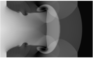
Figures 13(a) and 13(b) show the comparison between the experimental shadowgraph and the density contours obtained using simulations for the 6 and 10 mm shock tubes, respectively. From the observed contours, useful observations are made in the flow phenomena immediately after the diaphragm rupture is initiated. These figures closely explain the shock formation in practical scenarios where the shockwave forms at a finite distance from the diaphragm station due to the diaphragm's non-instantaneous rupture. The positions of the shock front and contact surface are captured with reasonable accuracy in the computations. It is seen that the initial shape of the shock front is spherical. The reflection of the spherical shock front from the walls leads to the formation of a Mach stem. Vortices are formed at the contact surface region that lead to mixing between the driver and driven gases. There are oblique structures between the shock front and the contact surface immediately after the diaphragm ruptures, catching up with the initial shock front. The shock front becomes planar at 63  $\mathrm {\mu }$s (corresponds to $t^*=3.6$) for the 6 mm shock tube and at 108 $\mathrm {\mu }$s (corresponds to $t^*=3.7$) for the 10 mm shock tube. Therefore, the shockwave in the two shock tubes becomes planar at the same dimensionless time. The shape of the shock front observed in the 10 mm shock tube case is captured well in the computations. Figure 13(c) shows the comparison of 6 and 10 mm shock tube simulations at the same $t^*$ after the simulation start. The wave phenomena behind the shock front are similar for both 6 and 10 mm shock tube cases at the same $t^*$ values. The similarity highlights that analogous flow features are observed at the same dimensionless time stamps. Figure 14(a) shows a snapshot of the density contour obtained in the simulation for the 10 mm shock tube. The formation of the triple point and the Mach stem is evident in the figure. The height of the Mach stem ( $h_m$) is also indicated. The trajectory of the triple point and the height of the Mach stem are measured in the simulations. The scaled Mach stem height, $h_m/D$, increases proportionally with the dimensionless parameter, $x/D$, for both the 6 and 10 mm shock tube cases (see figure 14b). Therefore, the shock formation process for the different diameters can be correlated based on the scaled parameters. The derivation of the correlation is elaborated in the following section. Figure 15 shows the variation of the shock Mach number along the driven section of the shock tube in the experimental and computational results. The shockwave location is tracked in the computational results based on the pressure jump at the shock front. The shock Mach number is computed from the location of the shockwave at different time instants. The shock Mach numbers at the shock formation distance predicted by the numerical simulations are similar to those observed in the experiments. These numerical simulations show that the wave interactions dominate the shock formation process resulting from the shock tube wall reflections.
Comparison of the experiments and simulations for the (a) 6 mm shock tube and (b) 10 mm shock tube. (c) Comparison between the computational fluid dynamics (CFD) results for the 6 and 10 mm shock tubes;  $P_{41} = 15$ and nitrogen is driver gas.

(a) Density contour of the 10 mm shock tube showing the Mach stem and triple point. The Mach stem height,  $h_m$, is indicated in the figure. (b) Plot comparing the growth of the Mach stem in the 6 and 10 mm shock tubes.

Comparison between the shock Mach number obtained from experiment and CFD simulations for (a) the 10 mm shock tube and (b) the 6 mm shock tube.

Figure 16 shows the flow features very close to the diaphragm based on the experimental and computational observations. As soon as the diaphragm opens/tears from the centre, the high-pressure driver gas gushes into the low pressure-driven gas, preceded by a shock wave that expands spherically in the space bounded by the walls of the shock tube (see figure 16a). The spherical nature of the shock front is attributed to a small portion of the diaphragm being opened. The spherical shock front expands in all directions inside the tube and reflects off the shock tube wall (see figure 16b). The flow of high-pressure driver gas past the partially opened diaphragm into an initially stationary low-pressure gas leads to the formation of counter-rotating vortex rings. The reflected shock moves towards the axis and interacts with the curved contact surface, vortex rings and the shocked gas region. The regular reflection of the reflected wave transforms into a Mach reflection as it catches up with the initial curved shock front, as shown in figure 16(c). Such a reflection leads to the formation of a Mach stem and a triple point. This phenomenon is similar to flow features observed when spherical shockwave reflections occur on interaction with a flat surface (Ben-Dor Reference Ben-Dor2007). A typical example is when explosions occur at a specific height from the ground, and the blast wave interacts with the surface (Needham Reference Needham2010). The vortex rings formed at the contact surface become larger and move towards the shock tube wall. This phenomenon leads to mixing the driver and the driven gases as more low-pressure gas gets trapped behind the enlarging vortex. As the diaphragm opens up completely, trailing vortices are formed at the contact discontinuity (see figure 16d). As time progresses, the Mach stem increases in height, the triple point moves closer to the centre of the shock tube, and the shock front becomes planar. When the triple points from opposite sides of the flow meet, the reflected waves interact and form a wave system of weak compression waves that eventually catch up with the moving shock front. The shock front accelerates in the shock formation phase until the transverse wave reflections die down, and vortices at the contact discontinuity are shed. Quantitative velocity measurements and robust simulations planned in the future will help in validating these findings.
Schematic diagrams showing the flow evolution and formation of the shockwave in the driven section as the diaphragm progressively opens from the centre of the shock tube.

4.2. Correlation to predict shock Mach number in shock formation region
The comparison between the experimental results and computations shows that the shock formation process is dominated by wave interactions due to the finite time for diaphragm rupture. The effect of the diaphragm's finite rupture time is that there are many reflected waves as a result of the initial compression wave from the diaphragm location that coalesces to form a single shock front. The first compression wave originating from the diaphragm location travels at the sound speed in the driven gas, i.e.  $a_1$. The shock front keeps gaining speed as it propagates down the tube as compression waves catch up. Therefore, the velocity of the shock front very close to the diaphragm location is $a_1$. Therefore, the minimum value of the shock front in the shock formation region is $a_1$. The increment in the shockwave velocity is dependent on initial conditions of the gases present on either side of the diaphragm, physical length scales and the mechanical properties of the diaphragm. The dependent quantities are:
(i) diameter of the shock tube ( $D$);
$D$);(ii) pressure in the driver and driven section (
$P_4$ and $P_1$);(iii) speed of sound in the driver gas (
$a_4$) and driven gas ($a_1$);(iv) diaphragm opening time (
$t_{op}$); and(v) shock formation distance (
$x_f$).


The diaphragm opening time is dependent on the material properties of the diaphragm and the initial pressure difference across the diameter. To understand the variation of the shockwave velocity with these parameters, experimental data reported by Rothkopf & Low (Reference Rothkopf and Low1976), Ikui et al. (Reference Ikui, Matsuo and Yamamoto1979) and Ikui & Matsuo (Reference Ikui and Matsuo1969) are considered along with the present experimental findings in the 2, 6 and 10 mm shock tubes. Table 2 shows the consolidated data for all the experimental conditions. The parameter  $a_{41}$ is the ratio of $a_4$ and $a_1$. The increase in shockwave velocity may be represented in terms of the dependent quantities in the following manner:
 \begin{equation} V_{Smax}-a_1 = f(x_f,D,P_{41},a_1t_{op},a_{41}). \end{equation}
Comparison between values predicted by correlation and experimentally obtained values in shock formation region.

The term  $a_1t_{op}$ represents the distance travelled by a compression wave with a velocity equal to the speed of sound in the driven gas. This characteristic distance helps represent the diaphragm opening time in terms of a length scale. The experimental results of Rothkopf & Low (Reference Rothkopf and Low1976) help in finding the variation of the quantities $a_1t_{op}$ and $a_{41}$ with $V_{Smax}$ while other parameters are kept constant. Similarly, Ikui et al. (Reference Ikui, Matsuo and Yamamoto1979) gives the variation of $P_{41}$ with $V_{Smax}$ when the other parameters are kept constant. Once these relationships are determined, the variation of $x_f$ with $V_{Smax}$ can also be found. It is seen that $V_{Smax}$ is directly proportional to $x_f$
$x_f$  $P_{41}$ $a_{41}$ but inversely proportional to $a_1t_{op}$. As a result of this analysis and combining the terms, the relationship between the quantities can be written as
 \begin{equation} \frac{V_{Smax}-a_1}{a_1} = f\left(\frac{x_f}{D},P_{41},\frac{D}{a_1t_{op}},a_{41}\right). \end{equation}
From figure 11, the variation of the shockwave velocity with distance is observed to follow a parabolic trend in the shock formation region. The quantities in the previous equation may be considered to follow a power relationship and the relation can be written as
 \begin{equation} \frac{V_{Smax}-a_1}{a_1} = A\cdot \left(\frac{x_f}{D}\right)^{C1}\cdot (P_{41})^{C2}\cdot \left(\frac{D}{a_1t_{op}}\right)^{C3}\cdot (a_{41})^{C4}, \end{equation}
where  $A$ is constant of proportionality and $C1$,
$C1$,  $C2$,
$C2$,  $C3$,
$C3$,  $C4$ are power constants. The values of the power constants are determined by substituting the values of the quantities given in table 2. After determining the values of the constants, (4.4) is given by
 \begin{equation} M_{Smax}-1 = A\cdot \left(\frac{x_f}{D}\right)^{0.5}\cdot (P_{41})^{0.1}\cdot \left(\frac{D}{a_1t_{op}}\right)^{0.4}\cdot a_{41}, \end{equation}
where the value of the constant  $A$ lies in the range 0.08–0.37. The performance of (4.5) with previously reported results is shown in table 2. The scatter in the value of the constant $A$ is reasonable, considering the wide range of supplementary variables shown in the table. The performance of this correlation with experimentally observed shock Mach number at different locations in the driven section of the shock tubes is reported in § 6.
5. Shock propagation region in the shock tube
5.1. Attenuation due to wall effects
The one-dimensional inviscid shock tube theory is routinely used for calculating the various output shockwave parameters when the underlying assumptions are valid, for example, in large shock tubes. However, this theory does not predict the fluid properties accurately in miniature shock tubes. Nonetheless, the values of the shockwave parameters obtained from experiments in the present work are compared with those obtained from the one-dimensional inviscid shock tube theory to observe the trends. Figure 17 shows the experimental results plotted against the prediction of the one-dimensional inviscid shock tube theory for all the three shock tube and driver gas configurations. The data points for the 2 mm shock tube are farther away from the ideal shock relations as compared to the 6 mm and the 10 mm cases (see figure 17a). Therefore, as the internal cross-section is reduced from 10 to 2 mm, a higher diaphragm pressure ratio is required to achieve the same particular shock Mach number. From figure 17(c), it is also evident that as the internal cross-section is reduced, a higher diaphragm pressure ratio is required to achieve the same pressure behind the shockwave. Figure 17(e) shows that in the 6 and 10 mm shock tubes, the ratio  $P_{21}$ increases with the shock Mach number. Similar observations are made when helium is used as the driver (see figures 17b, 17d and 17f). The relation between $P_{21}$ and $M_S$ matches the predictions of ideal theory (except for higher $M_S$ in the 10 mm case). These observations show that the experimental findings match the expected trends in miniature shock tubes.
Variation of the measured shockwave parameters. (a,c,e) Results for nitrogen driver. (b,d,f) Results for helium driver. The predictions of the 1-D inviscid shock tube theory are also indicated by the solid lines in the graphs.

The attenuation of shockwaves due to boundary layer development is well known and has been researched for many decades. The development of a scaling parameter has been explored numerically and experimentally for shockwave propagation through microchannels (Brouillette Reference Brouillette2003). This model accounts for the effect of length scales through molecular diffusion phenomena by parameterizing the shear stress and heat flux at the shock tube wall. As proposed by Brouillette (Reference Brouillette2003), the scaling parameter is defined as  $Re'\cdot D/4L$ where $Re'$ is the characteristic Reynolds number, and $L$ is the characteristic length. The characteristic length is defined as the distance between the shockwave and the contact surface. The 1-D shock relations are used to find the distance between the contact surface and the shockwave for the present experiments’ initial conditions. The scaling parameter values lie in the range of $175 < Scl < 5879$ for the present experimental conditions. Figure 18(a) compares the predictions for different values of the scaling parameter. It is clear that, for $Scl > 100$, the model is the same as the one-dimensional inviscid shock tube theory. Figures 18(b), 18(c) and 18(d) show the experimentally obtained variation of $P_{21}$ with $M_S$ as compared to the predictions using Brouillette's model for the 2, 6 and 10 mm shock tubes, respectively. In reality, the distance between the contact surface and the shock front is less than the value given by one-dimensional shock relations. Therefore, the scaling parameter is higher than the values taken for the present analysis. It is observed that Brouillette's model is closer to the ideal theory for large values of the scaling parameter. Therefore, the shockwave attenuation cannot be predicted by the model proposed by Brouillette (Reference Brouillette2003) when the scaling parameter is greater than 100, and the shock formation region is present in the shock tube.
Plots showing the relation between  $P_{21}$ and $M_S$. (a) Comparison of Brouillette's model for different values of scaling parameter. (b) Results for the 2 mm shock tube. (c) Results for the 6 mm shock tube. (d) Results for the 10 mm shock tube.

Using the scaling parameter, Zeitoun (Reference Zeitoun2015) presented a power law correlation to predict of attenuation in the shock Mach number in laminar and turbulent flows in a shock tube. The relation is given by
 \begin{equation} -\left(\frac{M_S-M_S^i}{M_S^i}\right)= C_a(Scx)^B, \end{equation}
where  $M_S^i$ corresponds to the initial shock Mach number, $C_a$ is the attenuation parameter, $Scx$ is the local scaling ratio and $B$ is $-$1/7 for the turbulent flow regime. The local scaling ratio is a function of the local position of the shockwave $x$ given by $Scx=(Re'D)/4x$. It was reported that the attenuation parameter gradually increases from zero to a value of 0.6, where maximum attenuation occurs. The maximum attenuation occurs at a distance that corresponds to 200 diameters. For the present scenario, it is observed that the shockwave velocity increases until the shock formation distance and subsequently decreases. Therefore, if the shock propagation region is defined as the region where the wall effects dominate the attenuation, then the shockwave's initial velocity can be taken equal to the maximum shock velocity reached during the end of the shock formation region. The correlation in (5.1) can be modified appropriately to support this assumption. The derivation and performance of the modified correlation are presented in the subsequent section.
5.2. Correlation to predict shock Mach number in propagation region
As mentioned in the previous section, the maximum Mach number attained by the shockwave at the end of the shock formation region is considered as the starting point for the correlation that is developed for the shock propagation region. Therefore, (5.1) is modified as follows:
 \begin{equation} M_S=M_{Smax}(1-C_a\cdot (Scx)^B),\end{equation}
where  $M_S$ represents the Mach number of the shockwave in the propagation region, $M_Smax$ is the peak Mach number reached by the shockwave at the end of the shock formation region, $C_a$ is the attenuation parameter and $B$ is $-$1/7; $Scx$ in (5.2) is the scaling parameter at the local position of the shockwave represented by $Scx=(Re'D)/(4(x-x_f))$, where $x_f$ is the shock formation distance. The local scaling parameter is changed because the shockwave's effective distance in the propagation region is $(x - x_f)$. The correlation between the velocity and the shockwave's local position, as represented in (5.2), is used to compare with the experimental data. The experimental data presented by Shtemenko and reported in Ikui & Matsuo (Reference Ikui and Matsuo1969) are also used for comparison. Table 3 shows the values of the Mach number obtained using the experimentally measured pressure signals and compares them with those computed using the correlation. The value of $x$ that corresponds to the first pressure transducer's location in the driven section is used. It is observed that the attenuation parameter takes values in the range of 0.30–0.37 for the experimental data. It was reported that the value of the attenuation parameter increases from zero to a value of 0.6 within about 300 times the tube diameter for a turbulent flow regime. It can be seen in the table that $(x - x_f)/D$ lies within 300. Therefore, the values of 0.30–0.37 are reasonable. Another important point is that the value of the attenuation parameter increases with the scaled distance. Therefore, the correlation between shock Mach number and local position of the shockwave represented in (5.2) works well for the propagation region.
Comparison between values predicted by correlation and shock Mach number obtained experimentally using pressure transducers.

6. Discussion
The relations represented in (4.5) and (5.2) are used to predict the shock Mach number at different locations in the driven section plotted in figure 11. Equation (4.5) can be represented in terms of the local position of the shockwave  $x$ as follows:
 \begin{equation} M_{S}-1 = A\cdot \left(\frac{x}{D}\right)^{0.5}\cdot (P_{41})^{0.1}\cdot \left(\frac{D}{a_1t_{op}}\right)^{0.4}\cdot a_{41}.\end{equation}
 Figures 19(a), 19(b) and 19(c) show the total attenuation in shock Mach number as predicted by the correlations developed for the shock formation and the shock propagation regions for the 10, 6 and 2 mm shock tubes. The correlation curves are obtained using the particular value of  $C_a$ for each shock tube (shown in table 3) and substituting the value of $x$ along the length of the driven tube. The shock formation distance is also indicated in the plots. The correlations predict the trend in the shock Mach number variation for all the shock tubes very well. Figure 19(d) shows the comparison of the variation of the shock Mach number along the driven section for the three shock tubes. An important observation is that the acceleration of the shock front is highest in the 2 mm shock tube and lowest in the case of the 10 mm shock tube during the shock formation process. The results are consistent with those obtained in the simulations in § 4, which showed that the shock front travels faster in the 6 mm shock tube as compared to the 10 mm shock tube. Since the shock formation distance is small in the 2 mm shock tube as compared to the other two hydraulic diameters, the peak Mach number of the shockwave is less for the 2 mm shock tube than the other shock tubes. This observation shows the decrement in the shock Mach number in the shock formation region compared to the value predicted by the one-dimensional inviscid shock relations. The value of the shock Mach number predicted by the one-dimensional inviscid theory is 1.73. There is a steep drop in the velocity initially in the shock propagation region, as a gradual change in the attenuation parameter is not considered while plotting the correlation. But overall, the prediction of the shock Mach number in experiments using the developed correlations is satisfactory. The predictions using the correlations are mainly limited because the shock formation distance is not known a priori, but is determined experimentally. A theoretical or empirical relationship to determine the shock formation distance accurately improves the predictions using the correlations. Thus, the flow in the miniature shock tubes can be divided into two regions: the shock formation region and the shock propagation region. The shock formation region is dominated by the wave reflections from the walls of the shock tube. The viscous effects are minimal in this region. The main parameters influencing the flow in this region are the hydraulic diameter of the shock tube ( $D$), diaphragm pressure ratio ( $P_{41}$), the speed of sound in the driver and driven gases ( $a_4$ and $a_1$), the diaphragm opening time ( $t_{op}$) and the shock formation distance ( $x_f)$. The shock propagation region is dominated by the viscous effects and the boundary layer's development behind the shock front.
Plots showing the comparison of the correlation with the experimental data points in the driven section of the (a) 10 mm shock tube, (b) 6 mm shock tube and (c) 2 mm shock tube. (d) A plot showing the distance–time graph of the shockwave trajectory obtained from correlations in the 10, 6 and 2 mm shock tubes;  $P_{41}=15$ and nitrogen is used as the driver gas.

7. Conclusions
A new table-top miniature shock tube system has been developed to understand the shock tube flow in 2, 6 and 10 mm square cross-section shock tubes. This study gives more in-depth insights into the shockwave attenuation due to the shock formation and the shock propagation processes. The shock tubes are run at pressure ratios in the range 5–25 and driven section at initial ambient conditions so that the operating conditions are similar to those used in shockwave-assisted applications. Nitrogen and helium are used as driver gases to calibrate the shock tubes. The results from the experiments are compared with various numerical, empirical and analytical models. The best agreement is obtained for an improved model suggested by Glass and Martin where the shockwave attenuation occurs in the two independent regions in the shock tube. (i) The formation of the shockwave is dominated by waves generated due to the finite rupture time of the diaphragm and their reflections from the walls of the shock tube. The wave interactions happen in the smaller diameter shock tube earlier than in larger diameter shock tubes. The scaled Mach stem height increases proportionally with the scaled distance along the shock tube length for different diameter shock tubes. (ii) After reaching the peak Mach number during the formation process, the propagation of the shockwave undergoes attenuation due to the formation of a turbulent boundary layer. The experimental findings indicate that the wave interactions and shock formation occur at the same dimensionless time in the shock tubes. Also, the maximum shock Mach number, which is reached at the shock formation distance, is higher for the 10 mm shock tube case than the 2 mm shock tube. New correlations have been developed to predict the shock Mach number in the shock formation and shock propagation region. Future experiments using the particle image velocimetry technique are planned to give valuable quantitative data close to the diaphragm station in the driver and driven sections. Also, large eddy simulation and direct numerical simulation studies of the shock tube flow due to the diaphragm's finite opening time will help validate the observations and experiments.
Acknowledgements
The authors would like to acknowledge the research grants from Defense Research and Development Organization, India, towards this study. The authors are also grateful to the members of the Laboratory for Hypersonic and Shockwave Research (LHSR), Department of Aerospace Engineering, Indian Institute of Science, for their support and help during this study.
Declaration of interests
The authors report no conflict of interest.
Supplementary movies
Supplementary movies are available at https://doi.org/10.1017/jfm.2020.914.
Appendix
Table 4 shows the experimental results for different initial driver pressures for the 2, 6 and 10 mm square cross-section shock tubes when the driver gas is nitrogen. Table 5 shows the experimental results for different initial driver pressures for the 2, 6 and 10 mm square cross-section shock tubes when the driver gas is helium.
Experimental results for different pressure ratios ( $P_{41}$) and nitrogen driver.

Experimental results for different pressure ratios ( $P_{41}$) and helium driver.


 Open access