2. Entropy in non-equilibrium open systems with flows

The standard definitions of entropy in statistical mechanics, such as $\ln \varGamma$ in an isolated system, where $\varGamma$ is the number of available microscopic states, or as the sum over all available microscopic states $-\sum _a p_a\ln p_a$ , where $p_a$ is the probability of the microscopic state $a$ , are applicable in the standard static statistical ensembles (Reichl Reference Reichl2009). The extension of the definition of entropy in non-equilibrium open systems with flows should be consistent with the standard definitions. For completeness, we briefly outline here the procedure of such an extension. Consider an ideal gas in a thermodynamic equilibrium. The entropy per particle is (Reichl Reference Reichl2009)

(2.1) \begin{align} \sigma &=\frac {5}{2}-\ln \!\left(n\lambda _T^3\right)\! , \\[-10pt] \nonumber \end{align}

(2.2) \begin{align} n&=\frac {N}{V,} \quad \lambda _T=\frac {h}{\sqrt {2\pi mT}} ,\\[8pt] \nonumber \end{align}

where $N$ is the number of particle, $V$ is the volume,  $h$ is the Planck constant, $m$ is the particle mass, $T$ is the temperature and $n$ is the number density. Let

(2.3) \begin{align} &\mathcal{P}=\frac {N\exp {(-{p^2}/{2mT})}}{\int \exp (-{p^2}/{2mT})\text{d}^3\boldsymbol{r}\text{d}^3\boldsymbol{p}/h^3}=n\lambda _T^3\exp \left(-\frac{p^2}{2mT}\right)\! , \end{align}

where we used $\int \text{d}^3\boldsymbol{r}=N$ . Note that

(2.4) \begin{align} &\int \mathcal{P}\text{d}^3\boldsymbol{p}=nh^3.\end{align}

Consider now the expression

(2.5) \begin{align} s &=-\int \mathcal{P}(\ln \mathcal{P}-1)\frac {\text{d}^3\boldsymbol{p}}{h^3} \\[-10pt] \nonumber \end{align}

(2.6) \begin{align} &=-\int \mathcal{P} \left (-\frac {p^2}{2mT}+\ln \big(n\lambda _T^3\big) -1\right )\frac {\text{d}^3\boldsymbol{p}}{h^3}\\[-10pt] \nonumber \end{align}

(2.7) \begin{align} &=\frac {5}{2}n-n \ln \big(n\lambda _T^3\big)=n\sigma , \\[8pt] \nonumber \end{align}

which is the entropy density and $w=-\mathcal{P}(\ln \mathcal{P}-1)/h^3$ is the phase-space entropy density.

Let now $f(\boldsymbol{r},\boldsymbol{p},t)$ be a single-particle distribution function such that

(2.8) \begin{align} &\int f(\boldsymbol{r},\boldsymbol{p},t)\text{d}^3\boldsymbol{p}=n(\boldsymbol{r},t). \end{align}

The distribution function $f(\boldsymbol{r},\boldsymbol{p},t)$ is the generalisation of the equilibrium $\mathcal{P}(\boldsymbol{p})$ .

Then the phase-space entropy density $w$ and the entropy density $s$ in a non-equilibrium system, described by a single-particle distribution function $f$ , can be defined as follows:

(2.9) \begin{align} w = -f(\ln (h^3f)-1) , \end{align}

(2.10) \begin{align} s(\boldsymbol{r},t) = -\int f(\ln (h^3f)-1)\text{d}^3\boldsymbol{p}=-\int f\ln (h^3f)\text{d}^3\boldsymbol{p}+n(\boldsymbol{r},t) .\end{align}

Accordingly, the entropy per particle would be

(2.11) \begin{align} &\sigma (\boldsymbol{r},t)= 1 - \frac {1}{n} \int f \ln (h^3f) \text{d}^3 \boldsymbol{p} .\end{align}

These expressions are more precise definitions of the usually used Boltzmann entropy (Parks et al. Reference Parks2012; Liang et al. Reference Liang2019; Du et al. Reference Du, Zank, Li and Guo2020; Agapitov et al. Reference Agapitov, Krasnoselskikh, Balikhin, Bonnell, Mozer and Avanov2023). The total entropy within a certain volume is

(2.12) \begin{align} &S=\int s\text{d}^3\boldsymbol{r}=\int n\sigma \text{d}^3\boldsymbol{r} .\end{align}

3. Conservation of Boltzmann entropy

The collisionless Vlasov equation is

(3.1) \begin{align} \frac {\partial f}{\partial t}+\boldsymbol{v}\boldsymbol{\cdot }\frac {\partial f}{\partial \boldsymbol{r}}+q\left (\boldsymbol{E}+\frac {1}{c}\boldsymbol{v}\times \boldsymbol{B}\right )\boldsymbol{\cdot }\frac {\partial f}{\partial \boldsymbol{p}} = 0 , \end{align}

which alternatively reads

(3.2) \begin{align} &\frac {\text{d}f}{\text{d}t}=0 \end{align}

along the trajectory $\dot {\boldsymbol{r}}=\boldsymbol{v}$ , $\dot {p}=q(\boldsymbol{E}+({1}/{c})\boldsymbol{v}\times \boldsymbol{B})$ . For each function $F(f)$ such that $F(f=0)=0$ we get

(3.3) \begin{align} &\frac {\text{d}F}{\text{d}t}=\left (\frac {\text{d}F}{\text{d}f}\right )\left (\frac {\text{d}f}{\text{d}t}\right )=0 , \end{align}

that is

(3.4) \begin{align} &\frac {\partial F}{\partial t}+\boldsymbol{v}\boldsymbol{\cdot }\frac {\partial F}{\partial \boldsymbol{r}}+\frac {q}{m}\left (\boldsymbol{E}+\frac {1}{c}\boldsymbol{v}\times \boldsymbol{B}\right )\boldsymbol{\cdot }\frac {\partial F}{\partial \boldsymbol{v}}=0 .\end{align}

Taking the lowest moment one has

(3.5) \begin{align} &\frac {\partial }{\partial t} \left (\int F(f(\boldsymbol{p},\boldsymbol{r},t))\text{d}^3\boldsymbol{p}\right )+ \frac {\partial }{\partial \boldsymbol{r}}\boldsymbol{\cdot }\left (\int \boldsymbol{v} F(f(\boldsymbol{p},\boldsymbol{r},t))\text{d}^3\boldsymbol{p}\right )=0 .\end{align}

In the stationary one-dimensional case, where everything depends only on the $x$ -coordinate, one has

(3.6) \begin{align} &\int v_x F(f(\boldsymbol{p},x))\text{d}^3\boldsymbol{p}=\text{const} .\end{align}

In particular, if $F=-f(\ln (h^3f)-1)$ , the corresponding moment

(3.7) \begin{align} &s=-\int f(\ln (h^3f)-1) \text{d}^3\boldsymbol{p} \end{align}

is the entropy density and

(3.8) \begin{align} &\boldsymbol{j}_s=-\int \boldsymbol{v} f(\ln (h^3f)-1) \text{d}^3\boldsymbol{p} \end{align}

is the entropy flux density. Conservation of entropy means

(3.9) \begin{align} &\frac {\partial s}{\partial t}+\boldsymbol{\nabla } \boldsymbol{\cdot }\boldsymbol{j}=0 .\end{align}

Entropy production would mean the appearance of a positive source term on the right-hand side of (3.9)

(3.10) \begin{align} &\frac {\partial s}{\partial t}+\boldsymbol{\nabla } \boldsymbol{\cdot }\boldsymbol{j}=\left (\frac {\text{d}s}{\text{d}t}\right )_{source} \end{align}

with $(\text{d}s/\text{d}t)_{source}\gt 0$ , as required by the second law of thermodynamics. If the shock is one-dimensional and stationary, $(\partial /\partial t)=0$ and $ (\partial /\partial y)=(\partial /\partial z)=0$ , then (3.9) means $j_{s,x}=\text{const}$ , in the absence of entropy production. The entropy flux density is constant throughout.

Let $(\boldsymbol{r},\boldsymbol{p},t)$ be a solution of the equations of motion

(3.11) \begin{align} &\frac {\text{d}\boldsymbol{r}}{\text{d}t}=\boldsymbol{v}, \qquad \frac {\text{d}\boldsymbol{p}}{\text{d}t}=q\left (\boldsymbol{E}+\frac {1}{c}\boldsymbol{v}\times \boldsymbol{B}\right ) \end{align}

with the initial conditions $(\boldsymbol{r}_0,\boldsymbol{p}_0,t_0)$ . For a one-dimensional time-independent shock $f(\boldsymbol{p},x)=f_0(\boldsymbol{p}_0,x_0)$ .

Consider a thin tube of particles starting at $x_0$ with the velocities in the infinitesimal momentum volume $\text{d}\boldsymbol{p}_0$ around $\boldsymbol{p}_0$ , corresponding to $\boldsymbol{v}_0$ . Let this infinitesimal region be Liouville mapped to $\text{d}\boldsymbol{p}$ around $\boldsymbol{p}$ , corresponding to $\boldsymbol{v}$ , at $x$ . The infinitesimal incident flux at $x_0$ is

(3.12) \begin{align} &\text{d}j=v_{0x}f_0(\boldsymbol{p}_0,x_0)\text{d}^3\boldsymbol{p}_0 .\end{align}

The flux conservation means that the same flux crosses $x$

(3.13) \begin{align} &v_{x}f(\boldsymbol{p},x)\text{d}^3\boldsymbol{p}=\text{d}j , \end{align}

which gives

(3.14) \begin{align} &\text{d}^3\boldsymbol{p}=\left |\frac {v_{0x}}{v_x}\right |\text{d}^3\boldsymbol{p}_0 \end{align}

and therefore, for each function $F(f)$ one has $F(f(\boldsymbol{p},x))=F(f_0(\boldsymbol{p}_0,x_0))$ and

(3.15) \begin{align} &\int F(f(\boldsymbol{p},x)) \text{d}^3\boldsymbol{p}=\int F(f_0(\boldsymbol{p}_0,x_0))\left |\frac {v_{0x}}{v_x}\right |\text{d}^3\boldsymbol{p}_0\ne \int F(f_0(\boldsymbol{p}_0,x_0))\text{d}^3\boldsymbol{p}_0 .\end{align}

The entropy conservation requires $j_x=\text{const}$ throughout In general,

(3.16) \begin{align} s/n & =-\left [\int f_0\ln f_0\left |\frac {v_{0x}}{v_x}\right |\text{d}^3\boldsymbol{p}_0\right ]\bigg/\left [\int f_0\left |\frac {v_{0x}}{v_x}\right |\text{d}^3\boldsymbol{p}_0\right ] \\[-10pt] \nonumber \end{align}

(3.17) \begin{align} & \ne -\left [\int f_0\ln f_0 \text{d}^3\boldsymbol{p}_0\right ]\bigg/\left [\int f_0\text{d}^3\boldsymbol{p}_0\right ]=s_0/n_{0} \\[8pt] \nonumber\end{align}

and, therefore, $s_d/n_d\ne s_u/n_u$ . In the above integrals $\boldsymbol{p}$ and $\boldsymbol{v}$ are functions of $\boldsymbol{p}_0$ .

Often, analysis is done in dimensionless variables. The distribution function is also dimensionless then. Let the number density be normalised with $n_0$ , and the velocity with $v_0$ , that is,

(3.18) \begin{align} & n=Nn_0, \boldsymbol{v}=\boldsymbol{V}V_0 , \\[-10pt] \nonumber\end{align}

(3.19) \begin{align} &N=\int F \text{d}^3\boldsymbol{V} , \\[-10pt] \nonumber\end{align}

(3.20) \begin{align} &F=f\frac {m^3V_0^3}{n_0}. \\[8pt] \nonumber \end{align}

Then the entropy density is

(3.21) \begin{align} S = n_0 s & =-\int F \left (\ln \left( \frac {n_0h^3}{m^3V_0^2}F\right)\boldsymbol{V}-1\right )\text{d}^3\boldsymbol{V} \\[-10pt] \nonumber \end{align}

(3.22) \begin{align} & = - \int F\ln F \text{d}^3\boldsymbol{V} -N\ln \frac {n_0h^3}{em^3V_0^2} . \\[8pt] \nonumber \end{align}

The difference of the entropy densities $S_d-S_u$ may appear positive or negative depending on the normalisation. Therefore, it is less informative than the entropy per particle

(3.23) \begin{align} &\frac {S}{N}=-\frac {1}{N} \int F\ln F \text{d}^3\boldsymbol{V} -\ln \frac {n_0h^3}{em^3V_0^2} .\end{align}

The second term is constant and can be safely omitted when the variations of the entropy per particle are analysed. Similarly, the entropy flux is

(3.24) \begin{align} n_{0} \boldsymbol{j}_{s} & =-V_0 \int \boldsymbol{V} F \left (\ln \left ( \frac {n_0h^3}{m^3V_0^2}F\right )\boldsymbol{V}-1\right )\text{d}^3\boldsymbol{V} \\[-10pt] \nonumber\end{align}

(3.25) \begin{align} & = - V_{0}\int F\ln F \text{d}^3\boldsymbol{V}-\left (\ln \frac {n_{0}h^3}{em^3V_{0}^2}\right )N\boldsymbol{V} .\end{align}

Thus, the normalisation adds a constant term to the entropy per particle and a term proportional to the particle flux density to the entropy flux. Note that, in a local thermodynamic equilibrium, described by the shifted Maxwellian

(3.26) \begin{align} &f_M=n\left (\frac {m}{2\pi T}\right )^{3/2} \exp \left (-\frac {m(\boldsymbol{v}-\boldsymbol{V})^2}{2T}\right )\! , \end{align}

where $n$ , $\boldsymbol{V}$ and $T$ depend on $\boldsymbol{r}$ and $t$ , the entropy density and the entropy flux density are related by $\boldsymbol{j}_{s}=s\boldsymbol{V}$ . In the general case, however, $\boldsymbol{j}_{s}\ne s\boldsymbol{V}$ .

In the one-dimensional stationary case, the particle flux density is constant. Since we are interested in the changes across the shock front, in the subsequent numerical analysis, we address only the variable parts, that is,

(3.27) \begin{align} &\frac {s}{n}=-\frac {\int f\ln f \text{d}^3\boldsymbol{v}}{\int f \text{d}^3\boldsymbol{v}}=-\frac {\int f_0\ln f_0\left |({v_{0x}}/{v_x})\right |\text{d}^3\boldsymbol{v}_0}{\int f_0\left |({v_{0x}}/{v_x})\right |\text{d}^3\boldsymbol{v}_0} , \\[-10pt] \nonumber \end{align}

(3.28) \begin{align} &j_{sx}=-\int v_xf\ln f \text{d}^3\boldsymbol{v}=-\int v_xf_0\ln f_0\left |\frac {v_{0x}}{v_x}\right |\text{d}^3\boldsymbol{v}_0 , \\[8pt] \nonumber \end{align}

where we reversed the notation to the more convenient lower case. The normalisation here is arbitrary. Only the difference $s_d/n_d-s_u/n_u$ is meaningful. A non-zero difference $j_{sxd}-j_{sxu}$ would mean entropy production. In a collisionless shock $j_{sx}=\text{const}$ throughout the shock, so that $j_{sxd}=j_{sxu}$ . The standard Rankine–Hugoniot relations assume that the upstream and downstream plasmas are in local thermodynamic equilibrium and require $s_d/n_d\gt s_u/n_u$ (Landau, Lifshitz & Pitaevskiĭ Reference Landau, Lifshitz and Pitaevskiĭ1984; Landau & Lifshitz Reference Landau and Lifshitz1987).

4. An analytic example: electrostatic shock

An electrostatic shock is a one-dimensional jump in the potential, through which a plasma flows. If the potential is $\phi (x)$ , the energy of a particle $\epsilon ={mv^2}/{2}+q\phi$ is conserved in the collisionless regime. For each species $f=f(\epsilon )$ . Let the upstream distribution be a one-dimensional shifted Maxwellian

(4.1) \begin{align} &f_0(v_0)=\exp \left (-\frac {(v_0-V_u)^2}{2v_T^2}\right )\! .\end{align}

We use the freedom in normalisation to avoid keeping unnecessary constants. The energy conservation is

(4.2) \begin{align} &v_0=\sqrt {v^2 +2q\phi /m} , \end{align}

therefore

(4.3) \begin{align} &f(x,v)=\exp \left (-\frac {(\sqrt {v^2 +2q\phi /m}-V_u)^2}{2v_T^2}\right ) \end{align}

and

(4.4) \begin{align} &\sigma =\frac {1}{N} \int \left (\frac {(\sqrt {v^2 +2q\phi /m}-V_u)^2}{2v_T^2}\right )\exp \left (-\frac {(\sqrt {v^2 +2q\phi /m}-V_u)^2}{2v_T^2}\right ) \text{d}v \end{align}

(4.5) \begin{align} =\frac {1}{N} \int \left (\frac {((v_{0}-V_{u})^2}{2v_{T}^2}\right ) \exp \left (-\frac {(v_{0}-V_{u})^2}{2v_{T}^2}\right ) \frac {v_{0}}{v} \text{d} v_{0} , \\[-28pt] \nonumber \end{align}

(4.6) \begin{align} N =\frac {n}{n_0}=\int \exp \left (-\frac {(\sqrt {v^2 +2q\phi /m}-V_u)^2}{2v_T^2}\right ) \text{d}v \\[-28pt] \nonumber \end{align}

(4.7) \begin{align} =\int \exp \left (-\frac {(v_{0} -V_{u})^2}{2v_{T}^2}\right ) \frac {v_{0}}{v}\text{d}v_0 . \\[-15pt] \nonumber \end{align}

If $v_T\ll V_u$ then

(4.8) \begin{align} &\frac {n}{n_0}\approx \frac {V_u}{\sqrt {V_u^2-2q\phi /m}} , \\[-10pt] \nonumber\end{align}

(4.9) \begin{align} &\frac {\sigma }{\sigma _0}\approx \frac {V_u}{\sqrt {V_u^2-2q\phi /m}} . \\[8pt] \nonumber \end{align}

For $q\phi \lt 0$ one would have $\sigma \lt \sigma _0$ .

5. Test particle analysis

The equations of motion inside the shock transition are not integrable analytically, and there is no closed analytical expression, neither for $f(\boldsymbol{p},x)$ nor for $v_x(x,v_{0x,}x_0)$ . Instead, we trace ions across a model shock front by numerically solving the ion equations of motion in prescribed stationary electric and magnetic fields. The fields depend only on the coordinate $x$ along the shock normal. The Maxwellian distributed incident ions are traced across the shock front. There is a set of layers $x_i\lt x\lt x_i+\Delta x$ , $x_i=x_l+(i-1)\Delta x$ , $i=1,\ldots , N$ , for the numerical derivation of the moments of the distribution function. Each ion contributes to the moment in a layer as many times as it is found in the layer, which is $\Delta x/|v_x|$ for sufficiently narrow layers (the staying time method). Multiplying by the weight $|v_{0x}|$ accounts for the Jacobian $|v_{0x}|/|v_{x}|$ . In the numerical calculation of the moments, the staying time method accounts for the denominator $1/|v_x|$ , since each ion contributes $\Delta x/ |v_x|$ times, provided $\Delta x$ is sufficiently small. The incident flux is taken into account by the weight $|v_{0x}|$ assigned to each particle. The additional factor is simply

(5.1) \begin{align} &\ln f_0=-\left (\frac {(v_{0x}-1)^2+v_{0y}^2+v_{0z}^2}{2v_T^2}\right )\! .\end{align}

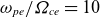
The focus of the study is the effect of the macroscopic stationary fields on the entropy, so that the shock model does not have to be self-consistent. We chose the model fields as follows:

(5.2) \begin{align} &B_{z} = \sin \theta _{Bn}\left (\frac {R+1}{2}+\frac {R-1}{2}{\tan}\textrm{h} \frac {3x}{D}\right )\! , \\[-10pt] \nonumber \end{align}

(5.3) \begin{align} &B_y=\frac {\cos \theta _{Bn}}{M_A}\frac {\text{d}B_z}{\text{d}x} ,\\[-10pt] \nonumber\end{align}

(5.4) \begin{align} &B_x=\cos \theta _{Bn} , \\[-10pt] \nonumber\end{align}

(5.5) \begin{align} &E_y=\sin \theta _{Bn} , \\[-10pt] \nonumber \end{align}

(5.6) \begin{align} &E_x=-l_E\frac {\text{d}B_z}{\text{d}z} , \\[-10pt] \nonumber\end{align}

(5.7) \begin{align} &E_z=0 . \\[8pt] \nonumber \end{align}

Here, the magnetic field $\boldsymbol{B}$ is normalised with the upstream magnetic field $B_u$ , the electric field $\boldsymbol{E}$ is normalised with $V_uB_u/c$ and the coordinate is normalised with the upstream convective gyroradius $V_u/\varOmega _u$ , $\varOmega _u=eB_u/m_pc$ . The coefficient $l_E$ is obtained from the condition $-\int E_x\,\text{d}x=\phi$ , where $\phi$ is the cross-shock potential normalised with $m_pV_u^2/2$ . The parameter $R$ is related to the magnetic compression ratio as follows:

(5.8) \begin{align} &\frac {B_d}{B_u}=\sqrt {R^2\sin ^2\theta _{Bn}+\cos ^2\theta _{Bn}} .\end{align}

Figure 1.

The magnitude of the model magnetic field.

Figure 2.

Left: the entropy flux density. Right: the entropy per particle.

The Alfvénic Mach number $M_A=V_u/v_A$ , where $v_A=B_u/\sqrt {4\pi n_um_p}$ is the Alfvén speed, the ramp width $D$ , the magnetic compression ratio $B_d/B_u$ , the shock angle $\theta _{Bn}$ and the cross-shock potential $\phi$ are the variable parameters of the model. In the following analysis $M_A=2$ , $B_d/B_u=1.9$ , $\theta _{Bn}=60^\circ$ and $D=1/M_A$ . The cross-shock potential $\phi$ and the incident ion $\beta _i=8\pi n_uT_u/B_u^2$ are varied. Figure 1 shows the magnitude of the model magnetic field. Figure 2 shows the entropy flux density $j_{sx}$ and the entropy per particle $s/n$ as a function of the coordinate along the shock normal, for $\beta _i=0.1$ and the normalised cross-shock potential $\phi =0.45$ . The flux is conserved, as expected. The entropy per particle also remains constant, $s_d/n_d=s_u/n_u$ . This may make an impression that the heating is adiabatic, in the sense that $n/T^{3/2}=\text{const}$ . However, adiabaticity implies thermodynamic equilibrium, while the downstream distribution is not Maxwellian. The amount of ion heating is roughly determined by $|\sqrt {1-\phi }-V_d|$ . The conservation of $s/n$ in this case is coincidental and due to the choice of the parameters.

Figure 3 shows the entropy flux density $j_{sx}$ and the entropy density $s$ as a function of the coordinate along the shock normal, for $\beta _i=0.1$ and the normalised cross-shock potential $\phi =0.65$ . The entropy flux is conserved. However, $s_d/n_d\gt s_u/n_u$ , although the difference is small. The larger cross-shock potential increases the dispersion of $|v_x|$ in the denominator of (3.27). Since the ions are decelerated at the shock crossing, this increase of the velocity dispersion causes the weak increase in $s/n$ .

Figure 3.

Left: the entropy flux density. Right: the entropy per particle.

Figure 4 shows the entropy flux density $j_{sx}$ and the entropy density $s$ as a function of the coordinate along the shock normal, for $\beta _i=0.5$ and the normalised cross-shock potential $\phi =0.45$ . The entropy flux is conserved. In this case, $s_d/n_d\gt s_u/n_u$ noticeably. This change occurs due to the larger dispersion of $|v_x|$ in the denominator of (3.27) for the higher initial thermal speed of the ions.

Figure 4.

Left: the entropy flux density. Right: the entropy per particle.

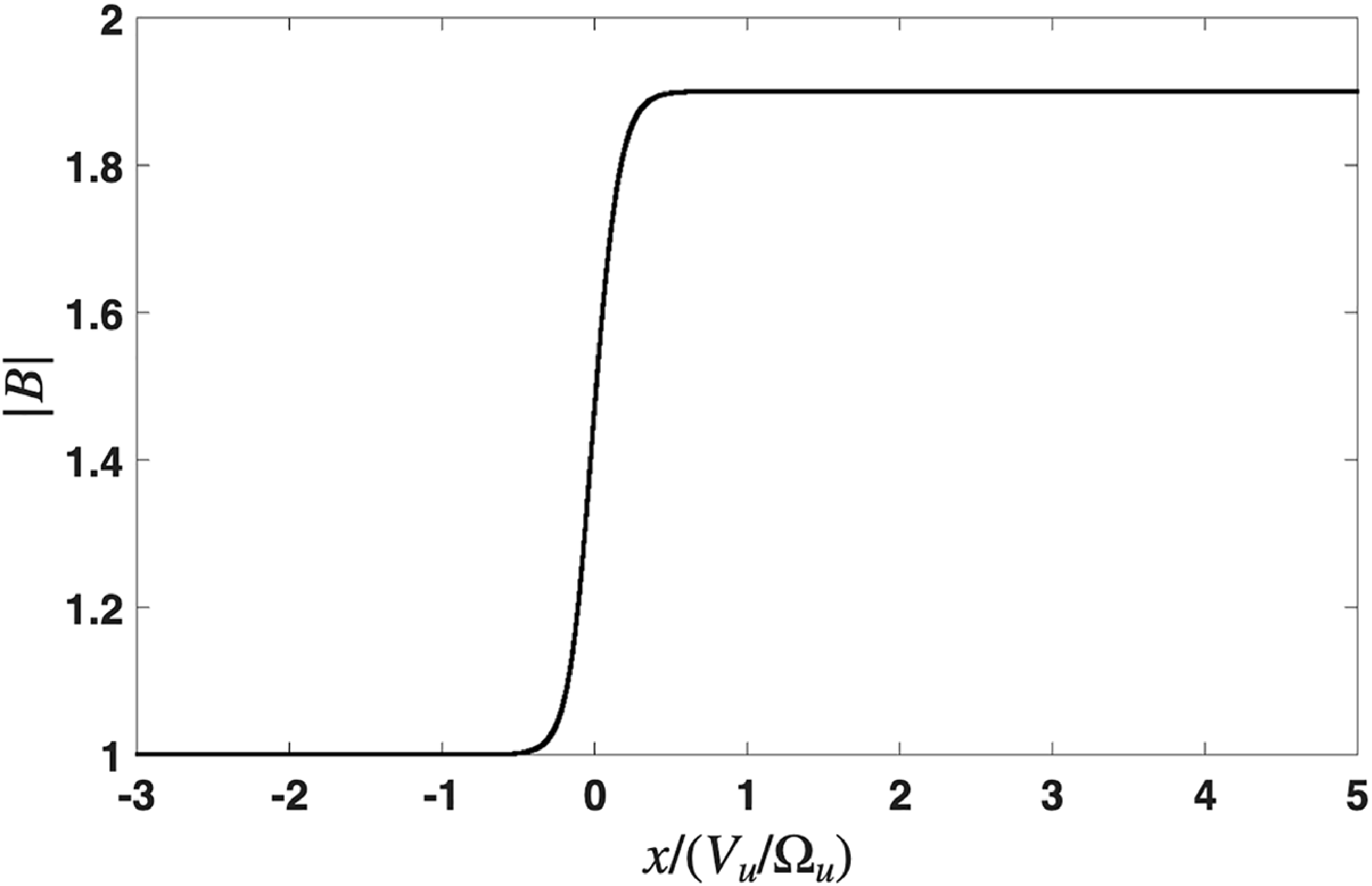
Figure 5 shows the results of a similar electron tracing across the same model shock. In contrast with ions, electrons are accelerated across the shock by the cross-shock potential. In addition, because of their small mass, the ratio of their upstream thermal speed to the shock speed $v_{Te}/V_u=\sqrt {m_i/m_e}\sqrt {\beta /2}/M_A$ is by the factor $\sqrt {m_i/m_e}$ larger than that of ions with the same $\beta$ . To reduce computational time, the mass ratio in the electron tracing was set to $m_e/m_i=1/100$ . In figure 5 the electron $\beta =0.05$ and $\phi =0.45$ . Figure 6 shows the results of another electron tracing across the same model shock. The electron $\beta =0.05$ and $\phi =0.65$ . Figure 7 shows the results of yet another electron tracing across the same model shock. This time the electron $\beta =0.025$ and $\phi =0.45$ . The entropy flux is conserved, while the entropy per particle decreases. The decrease in this case is related to the acceleration of the electrons across the shock front and small dispersion of $|v_x|$ in the denominator of (3.27).

Figure 5.

Left: the entropy flux density. Right: the entropy per particle.

Figure 6.

Left: the entropy flux density. Right: the entropy per particle.

Figure 7.

Left: the entropy flux density. Right: the entropy per particle.

Figure 8.

Top: the electron density and the magnetic field. Middle: the entropy per particle. Bottom: the entropy flux density. Left column: electrons. Right column: ions. Upstream is on the right, downstream is on the left.

6. Simulations

The above test particle analysis shows that entropy is strictly conserved in a time-independent planar shock. This conservation takes the form $\text{d}j_{s,x}/\text{d}x=0$ . On the other hand, the entropy per particle may increase or decrease, depending on the particle charge sign, cross-shock potential and the temperature of the upstream incident distribution. The test particle analysis does not take into account the field fluctuations, produced self-consistently by the charged particles. To understand the role of these fluctuations, we performed particle-in-cell (PIC) simulations.

The two-dimensional PIC simulation of a low-Mach-number shock presented here was performed using the VPIC code (Bowers et al. Reference Bowers, Albright, Yin, Bergen and Kwan2008). The shock is created by the reflection of plasma flowing in the negative $x$ direction from a rigid, perfectly conducting wall. The upstream distributions for both electrons and ions are Maxwellian, with density $n_0$ and temperatures $T_e$ and $T_i$ , respectively. The angle between the upstream magnetic field $B_0$ and the $x$ -axis is $\theta _{Bn} = 111^\circ$ . The upstream magnetic field is in the $xy$ plane. The plasma is injected from the right boundary of the domain at $x=L_x$ with the inflow speed $V_{in} = 1 V_A$ , where $V_A = B_0/\sqrt {4 \pi n_0 m_i}$ is the Alfvén speed. The shock moves in the positive $x$ direction with the average speed $V_{sh} = 1.42 V_A$ , such that the upstream flow in the shock frame $V_0$ is characterised by the Mach number $M_A = V_0/V_A = 2.42$ . The upstream $\beta _i = 0.3$ and $\beta _e=2.6$ , where $\beta _s = 8 \pi n_0 T_s/B_0^2$ and $s=e,i$ denotes plasma species. The simulation domain has dimensions $L_x \times L_y = (50 \times 5) d_i$ , where $d_s = c/\omega _{ps}$ , $c$ is the speed of light and $\omega _{ps} = ( 4 \pi n_0 e^2/m_s)^{1/2}$ . The domain is resolved by a uniform Cartesian grid with resolution $N_x \times N_y = 18\,816 \times 1984$ cells, such the cell size is approximately one Debye length in the upstream plasma. The mass ratio is $m_i/m_e=1836$ . The ratio between the electron plasma frequency $\omega _{pe}$ and the electron cyclotron frequency $\varOmega _{ce}$ is $\omega _{pe}/\varOmega _{ce}=10$ , where $\varOmega _{cs} = e B_0/(m_s c)$ . The simulation time step is $\delta t \omega _{pe} \approx 0.06$ .

To compute the entropy, $y$ -averaged distribution functions were accumulated on a three-dimensional velocity grid at regular intervals. The distributions were further averaged over a small interval $\delta x \approx 0.05 d_i$ . The velocity grid resolution was approximately $0.4V_A$ for electrons and $8.5\times 10^{-3} V_A$ for ions. The entropy density and the entropy flux were obtained by numerical integration of the reconstructed distribution over this grid. We have verified that the results are converged with respect to the resolution of the velocity-space grid. Figure 8 shows the results for the electrons (left column) and ions (right column) at time $t=19\varOmega _{ci}^{-1}$ . The top panel shows profiles of the density and magnetic field. The middle panel is the entropy density per particle, normalised to the upstream reference value $S_{0i} = n_0 [ 3/2 - \log n_0 + 3 \log (\sqrt \pi v_{ts}) ]$ , where $v_{ts}^2 = 2 T_s/m_s$ . Finally, the bottom panel shows the entropy flux for each species normalised to $V_0 S_{0s}$ . Multiple relatively small amplitude instabilities are present in the simulation, especially in the vicinity of the ramp. The influence of these fluctuations on the evolution of entropy per particle and entropy flux density is self-consistently accounted for. There is no substantial effect of the fluctuations on the entropy flux density, so that no significant entropy production is found.