


1. Introduction
A hydraulic jump occurs in the context of open-channel flow when a high-velocity, low-depth (supercritical) current transitions abruptly to a low-velocity, high-depth (subcritical) state. The transition is typically not smooth and is associated with energy dissipation. The main causes are: (i) a sudden increase in downstream depth; (ii) changes in channel geometry, such as an abrupt expansion in channel width, a drop in channel slope or an abrupt channel deviation; (iii) obstructions in the flow path induced by structures like weirs or sluice gates; (iv) abrupt decrease in bed slope; (v) a sudden increase in bed wall roughness; (vi) energy dissipation design, when a hydraulic jump is intentionally created in stilling basins to reduce flow energy; (vii) certain combinations of discharge, depth and channel shape leading to supercritical conditions that cannot be sustained, forcing a jump. An in-depth description of the hydraulic jump can be found in Bakhmeteff (Reference Bakhmeteff1932) and Chow (Reference Chow1959), while more recent reviews are Chanson (Reference Chanson2009) and De Padova & Mossa (Reference De Padova and Mossa2021).
Thus, a deflection of the channel axis, either abrupt or progressively curved, is a common cause of the hydraulic jump, especially in irrigation systems, such as the one considered in the pioneering study by Ippen (Reference Ippen1936). The sudden increase in water depth due to hydraulic jump in a sudden deflection or progressive superelevation on the concave side of a bent channel can lead to overspilling, thus representing the main technical obstacle. Other interesting applications concern the field of granular flow, as shown by Wieland, Gray & Hutter (Reference Wieland, Gray and Hutter1999) and Gray & Cui (Reference Gray and Cui2007); in particular, this type of flow can be applied to model snow avalanches, like in Cui, Gray & Johannesson (Reference Cui, Gray and Johannesson2007)’s case.
The earliest investigations into rapid flow within deflected channels were conducted by Prandtl (Reference Prandtl1931), Busemann (Reference Busemann1931), Riabouchinsky (Reference Riabouchinsky1932), Riabouchinsky (Reference Riabouchinsky1934) and Preiswerk (Reference Preiswerk1938) who emphasized the analogy between such flows and the supersonic gas dynamics, introducing a graphical solution method based on characteristic curves. Von Kármán (Reference Von Kármán1938) derived an expression for the increase in water depth along the concave side of a channel bend, assuming constant specific energy. In contrast, Ippen (Reference Ippen1936), Ippen & Knapp (Reference Ippen and Knapp1936) and Knapp & Ippen (Reference Knapp and Ippen1938) addressed the same problem under the assumption of constant velocity, leading to a different analytical solution. The specific case of an oblique hydraulic jump resulting from an abrupt channel deflection was first introduced by Rouse (Reference Rouse1938) and Ippen (Reference Ippen1943). A comprehensive review of earlier studies is provided by Citrini (Reference Citrini1940), Citrini (Reference Citrini1950), Rouse (Reference Rouse1959), Chow (Reference Chow1959), Levi (Reference Levi1965) and Press & Schröder (Reference Press and Schröder1966).
Ippen (Reference Ippen1936) conducted one of the most complete experimental investigations on supercritical flow in curved channels. His work was later complemented by Engelund & Munch-Petersen (Reference Engelund and Munch-Petersen1953), who analysed wave formation in converging and diverging channels. Poggi (Reference Poggi1956) performed a series of experiments in a curved channel to validate the analytical models proposed by Ippen (Reference Ippen1936) and von Kármán (Reference Von Kármán1938). The Poggi findings were subsequently referenced in the laboratory studies of Sananes & Acatay (Reference Sananes and Acatay1962) and Reinauer & Hager (Reference Reinauer and Hager1997). Finally, Marchi (Reference Marchi1988) presented experimental results for the limiting case of an abrupt $90^\circ$
channel bend, with further references to his work appearing in Solari & Dey (Reference Solari and Dey2016).
$90^\circ$
channel bend, with further references to his work appearing in Solari & Dey (Reference Solari and Dey2016).
More recently, Hager et al. (Reference Hager, Schwalt, Jimenez and Chaudhry1994) conducted a series of experimental tests, supported by numerical results based on a shallow-water framework. In a similar vein, Causon, Mingham & Ingram (Reference Causon, Mingham and Ingram1999) used shallow-water numerical simulations to evaluate the increase in depth of the water caused by an oblique shock wave. Beltrami, Repetto & Del Guzzo (Reference Beltrami, Repetto and Del Guzzo2007) conducted experiments with the practical aim of reducing superelevation near the channel wall and regularizing flow by installing water flaps along the wall.
The hydraulic jump in Newtonian fluids has been extensively studied, whereas research on non-Newtonian rheologies remains comparatively limited. A seminal study by Ng & Mei (Reference Ng and Mei1994) examined the properties and evolution of roll waves in power-law fluids, also theoretically analysed in Longo (Reference Longo2011).
Regarding fluid characterization, Haldenwang & Slatter (Reference Haldenwang and Slatter2006) and Burger, Haldenwang & Alderman (Reference Burger, Haldenwang and Alderman2010a ) compiled valuable experimental databases detailing the rheological behaviour of non-Newtonian fluids, specifically in straight channels with varying cross-sectional geometries.
In direct connection with hydraulic jumps, Shu & Zhou (Reference Shu and Zhou2006) and Zhou, Shu & Stansby (Reference Zhou, Shu and Stansby2007) investigated these phenomena in Bingham fluids flowing through straight channels. Unlike the classical Newtonian case, where analytical solutions for conjugate depths are readily available, their analysis led to systems of nonlinear algebraic equations, which required numerical methods for resolution. To address this, they proposed approximate formulae for estimating conjugate depths, thereby offering practical tools for engineering applications involving non-Newtonian flows. A similar methodology was adopted by Ugarelli & Di Federico (Reference Ugarelli and Di Federico2007) for Herschel–Bulkley fluids, including an example application based on experimental data from Haldenwang & Slatter (Reference Haldenwang and Slatter2006), regarding the flow of a $6\,\%$
kaolin suspension down an inclined rectangular flume.
$6\,\%$
kaolin suspension down an inclined rectangular flume.
More recently, Samanta et al. (Reference Samanta, Ray, Kaushal and Das2022, Reference Samanta, Kaushal, Das and Ray2023) presented analytical, numerical and experimental studies on hydraulic jumps in power-law fluids under planar conditions, using a shallow-water framework. Their approach was extended to Bingham plastics in Samanta et al. (Reference Samanta, Das, Ray and Kaushal2024a ) and to Herschel–Bulkley fluids in Samanta et al. (Reference Samanta, Kaushal, Das and Ray2024b ). Finally, Wang, Khayat & De Bruin (Reference Wang, Khayat and De Bruin2023) extended the analysis to Herschel–Bulkley fluids in circular geometries. However, to the authors’ knowledge, a comprehensive investigation of laminar hydraulic jumps in non-Newtonian fluids flowing through channels with abrupt deviations has yet to be undertaken. This gap is particularly notable given the relevance of such flows in environmental applications, such as modelling mud flows (Cui et al. Reference Cui, Gray and Johannesson2007), the conveyance or disposal of mine tailings in industrial waste management (Burger et al. Reference Burger, Haldenwang and Alderman2010b ), landslides, debris and lava flows. Furthermore, non-Newtonian fluids are prevalent in a wide range of industrial processes where deviations in free-surface channels may arise, including cooling and coating processes (Chimetta & Franklin Reference Chimetta and Franklin2023), foam cleaning (Dallagi et al. Reference Dallagi, Faille, Bouvier, Deleplace, Dubois, Aloui and Benezech2022) and food science in general (Mathijssen et al. Reference Mathijssen, Lisicki, Prakash and Mossige2023).
In this study, the laminar free-surface flow of a power-law (Ostwald–de Waele) fluid – the simplest and most widely used non-Newtonian rheological model – is examined in the presence of a geometric disturbance, namely an abrupt angular channel deflection, which can induce the formation of a hydraulic jump. Although idealized, the power-law model effectively captures the rheological behaviour of clay–water mixtures commonly found in natural settings such as landslides (Carotenuto et al. Reference Carotenuto, Merola, Álvarez-Romero, Coppola and Minale2015), estuarine muds (Zhang et al. Reference Zhang, Bai and Ng2020) and mine tailings (Borger Reference Borger2013). Field-scale applications of laminar flows adopting a power-law rheology have been reported by Haldenwang & Slatter (Reference Haldenwang and Slatter2006) for bentonite and kaolin suspensions and carboxymethylcellulose solutions, by Latkovic & Levy (Reference Latkovic and Levy1991) for fluidized magnetite powder, by Kozic et al. (Reference Kozic, Ristic, Linic, Hil and Stetic-Kozic2016) for soybean paste and by Kumbár et al. (Reference Kumbár, Kourilová, Dufková, Votava and Hrivna2021) for chocolate masses. Another example of laminar free-surface flow of a non-Newtonian fluid without yield-stress is provided by human and animal blood (Horner, Wagner & Beris Reference Horner, Wagner and Beris2021) or silicon-like material in injection moulding (Chiappini Reference Chiappini2020). Nevertheless, both assumptions of power-law rheology and laminar flow constitute limitations of the present work.
In the first case, many natural and industrial fluids, as well as contaminants, exhibit finite yield stress, with a rheological behaviour more accurately described by Bingham or Herschel–Bulkley constitutive models.
In the second case, it will be of considerable interest in future work to investigate the behaviour of non-Newtonian fluids in a transitional and fully turbulent regime. The evolution of their flow fields from laminar through transition to turbulence at high Reynolds numbers remains an open research problem. Significant differences are known to exist compared with Newtonian turbulence, and this area still requires fundamental investigation. For example, Guzel et al. (Reference Guzel, Burghelea, Frigaard and Martinez2009) reported pronounced asymmetries in turbulent puffs that were attributed to fluid rheology, although the mean flow was perfectly axisymmetric.
The overarching objective is to investigate the conditions leading to the formation and structure of hydraulic jumps in these flows, and more generally, to characterize the development of oblique shocks that include proper hydraulic jumps as a special case. To this end, three secondary objectives are pursued: (i) the development of a one-dimensional (1-D) analytical framework, based on the governing equations of mass conservation, momentum balance and power-law rheology, following the classical formulations by Ippen (Reference Ippen1936) and von Kármán (Reference Von Kármán1938); (ii) the design and execution of controlled laboratory experiments in inclined, laterally deflected channels aimed at observing the conditions for jump formation, the shock structures and the geometry of the Mach front (whether rectilinear or curved, detached or attached), preceded by rheological characterization of the fluid properties; (iii) extensive numerical simulations of diverse flow configurations, employing both a depth-averaged shallow-water model and a depth-resolved multiphase solver implemented in OpenFOAM.
The paper is organized as follows. Section 2 presents the geometrical set-up and simplified 1-D formulation of the problem, leading to the rheological equation and the uniform velocity profile. In § 3, a simplified flow analysis is conducted based on conservation principles, resulting in a nonlinear transcendental system of three algebraic equations with three unknowns. Section 4 details the laboratory experiments conducted in a tilted, laterally deflected channel. Numerical simulations are presented in § 5: a shallow-water formulation verifying experimental tests is presented first, then it is used to ascertain the validity of a 1-D formulation incorporating friction and bed slope. Section 6 illustrates the results of a depth-resolved solver implemented in OpenFOAM. A summary and comparative analysis of the results obtained from the analytical, experimental and numerical approaches is provided in § 7, which also includes conclusions and perspectives for future work.
2. One-dimensional formulation
A wide rectangular horizontal channel conveying an Ostwald–de Waele (hereafter power-law) fluid in a steady laminar regime undergoes an abrupt deflection of its axis by an angle $\theta$
, causing a perturbation of the flow conditions, as shown in figure 1. Variation in flow conditions occurs only downstream of a perturbation wave, originating at the vertex of the deflection and inclined by the Mach angle
$\theta$
, causing a perturbation of the flow conditions, as shown in figure 1. Variation in flow conditions occurs only downstream of a perturbation wave, originating at the vertex of the deflection and inclined by the Mach angle $\beta$
from the wall (Press & Schröder Reference Press and Schröder1966). The upstream and downstream conditions, indicated, respectively, with subscripts 1 and 2, are connected by this wavefront.
$\beta$
from the wall (Press & Schröder Reference Press and Schröder1966). The upstream and downstream conditions, indicated, respectively, with subscripts 1 and 2, are connected by this wavefront.
Geometry of the deflected channel and representation of the shock wave.

For a rectangular channel with depth $Y$
along the vertical
$Y$
along the vertical $z$
-direction (using the conventional hydraulic engineering notation
$z$
-direction (using the conventional hydraulic engineering notation $Y$
for depth, to ensure consistency with the literature and with the notation adopted in subsequent sections) where
$Y$
for depth, to ensure consistency with the literature and with the notation adopted in subsequent sections) where $Y\ll b$
(lubrication approximation) and
$Y\ll b$
(lubrication approximation) and $b$
is the channel width in the transverse
$b$
is the channel width in the transverse $y$
-direction, the transverse and vertical velocity components are negligible and the velocity vector is approximately
$y$
-direction, the transverse and vertical velocity components are negligible and the velocity vector is approximately $\boldsymbol {u}=(u,0,0)$
as
$\boldsymbol {u}=(u,0,0)$
as $\tau _{yx}\ll \tau _{zx}$
, where
$\tau _{yx}\ll \tau _{zx}$
, where $u$
is the velocity in the
$u$
is the velocity in the $x$
direction,
$x$
direction, $\tau _{yx}$
and
$\tau _{yx}$
and $\tau _{zx}$
are components of the shear stress tensor. The hydrostatic pressure distribution is also assumed, consistent with the lubrication approximation adopted earlier. Under these conditions, the rheological equation for a power-law fluid simplifies to the following 1-D form:
$\tau _{zx}$
are components of the shear stress tensor. The hydrostatic pressure distribution is also assumed, consistent with the lubrication approximation adopted earlier. Under these conditions, the rheological equation for a power-law fluid simplifies to the following 1-D form:
 \begin{equation} \tau _{zx}=-K\left |\frac {\partial u}{\partial z}\right |^{n-1}\frac {\partial u}{\partial z}, \end{equation}
where $K$
and
$K$
and $n$
are the consistency index and the fluid behaviour index, respectively. For
$n$
are the consistency index and the fluid behaviour index, respectively. For $n\lt 1$
, the fluid is shear-thinning (pseudoplastic); for
$n\lt 1$
, the fluid is shear-thinning (pseudoplastic); for $n=1$
, the fluid is Newtonian and
$n=1$
, the fluid is Newtonian and $K$
reduces to
$K$
reduces to $\mu$
, the dynamic viscosity; for
$\mu$
, the dynamic viscosity; for $n\gt 1$
, the fluid is shear-thickening (dilatant).
$n\gt 1$
, the fluid is shear-thickening (dilatant).
The channel is considered to have negligible wall and bottom effects; the velocity varies along the vertical, from a minimum at the bottom to a maximum at the free surface, with a distribution given by the following equation (Di Federico Reference Di Federico1998):
 \begin{equation} u(z)=u_{\textit{max}}\left [1-\left (1-\frac {z}{Y}\right )^{\frac {n+1}{n}}\right ]\!, \end{equation}
where $u_{\textit{max}}$
is the maximum velocity value at the free surface. The average velocity
$u_{\textit{max}}$
is the maximum velocity value at the free surface. The average velocity $V$
in the
$V$
in the $x$
direction is obtained by integrating the previous equation along the vertical direction
$x$
direction is obtained by integrating the previous equation along the vertical direction $z$
, resulting in
$z$
, resulting in
 \begin{equation} V=\frac {1}{Y}\int _0^Yu(z)\,\text{d}z=\left (\frac {n+1}{2n+1}\right )u_{\textit{max}}. \end{equation}
The Boussinesq coefficient $C_{\!M}$
, also termed the dimensionless momentum flux correction coefficient or shape factor, which accounts for the non-uniformity of the velocity profile in the vertical direction, can be calculated for a power-law fluid from (2.2) as (Ng & Mei Reference Ng and Mei1994)
$C_{\!M}$
, also termed the dimensionless momentum flux correction coefficient or shape factor, which accounts for the non-uniformity of the velocity profile in the vertical direction, can be calculated for a power-law fluid from (2.2) as (Ng & Mei Reference Ng and Mei1994)
 \begin{equation} C_{\!M}=\frac {\int _Au^2\,\text{d}A}{A\left (\frac {1}{A}\int _Au\,\text{d}A\right )^2}=\frac {2(2n + 1)}{3n + 2}, \end{equation}
where $A$
is the cross-sectional area.
$A$
is the cross-sectional area.
The problem studied here involves the determination of three unknowns: the depth of the downstream flow $Y_2$
, the angle of Mach
$Y_2$
, the angle of Mach $\beta$
and the average downstream velocity
$\beta$
and the average downstream velocity $V_2$
. The known quantities are the depth of the upstream flow
$V_2$
. The known quantities are the depth of the upstream flow $Y_1$
, the mean velocity
$Y_1$
, the mean velocity $V_1$
, the angle of deflection of the channel
$V_1$
, the angle of deflection of the channel $\theta$
and the rheological parameters
$\theta$
and the rheological parameters $K$
and
$K$
and $n$
. Flow conditions are conveniently characterized in terms of the Froude number
$n$
. Flow conditions are conveniently characterized in terms of the Froude number $\textit{Fr}$
:
$\textit{Fr}$
:
 \begin{equation} \textit{Fr}=\frac {V}{\sqrt {gY}}=\left (\frac {n+1}{2n+1}\right )\frac {u_{\textit{max}}}{\sqrt {gY}}, \end{equation}
where $g$
is the gravity. The Boussinesq coefficient
$g$
is the gravity. The Boussinesq coefficient $C_{\!M}$
defined in (2.4) is directly correlated to the critical Froude number
$C_{\!M}$
defined in (2.4) is directly correlated to the critical Froude number $\textit{Fr}_c$
for an Ostwald–de Waele fluid (Campomaggiore et al. Reference Campomaggiore, Di Cristo, Iervolino and Vacca2016), through the expression
$\textit{Fr}_c$
for an Ostwald–de Waele fluid (Campomaggiore et al. Reference Campomaggiore, Di Cristo, Iervolino and Vacca2016), through the expression
 \begin{equation} \textit{Fr}_C=1/\sqrt {C_{\!M}}. \end{equation}
For convenience in the subsequent analysis, we introduce the normalized Froude number $F_{*}=\textit{Fr}/\textit{Fr}_c=\textit{Fr}\sqrt {C_{\!M}}$
, i.e. the ratio of the Froude number to the critical Froude number.
$F_{*}=\textit{Fr}/\textit{Fr}_c=\textit{Fr}\sqrt {C_{\!M}}$
, i.e. the ratio of the Froude number to the critical Froude number.
It should be noted that in cases where the velocity profile in the vertical direction can be approximated as uniform, i.e. $C_{\!M} = 1$
, such as in turbulent clear water flows (Ippen Reference Ippen1936) or dense granular flows (Gray & Cui Reference Gray and Cui2007), the critical Froude number equals unity (
$C_{\!M} = 1$
, such as in turbulent clear water flows (Ippen Reference Ippen1936) or dense granular flows (Gray & Cui Reference Gray and Cui2007), the critical Froude number equals unity ( $\textit{Fr}_c = 1$
), and thus
$\textit{Fr}_c = 1$
), and thus $F_{*1}$
coincides with the Froude number
$F_{*1}$
coincides with the Froude number $\textit{Fr}_1$
. In contrast, for laminar flows of power-law fluids, the critical Froude number varies depending on the rheological properties of the fluid, specifically the power-law exponent
$\textit{Fr}_1$
. In contrast, for laminar flows of power-law fluids, the critical Froude number varies depending on the rheological properties of the fluid, specifically the power-law exponent $n$
.
$n$
.
2.1. Criterion for laminar flow
The criterion adopted here to verify the laminar flow follows the empirical method proposed by Darby (Reference Darby1986) and subsequently applied by Ng & Mei (Reference Ng and Mei1994). The flow is considered laminar if the wide-channel Reynolds number, defined as
 \begin{equation} \textit{Re} = \frac {\rho V^{2-n} Y^{n}}{K}, \end{equation}
where $\rho$
is the density of the fluid, remaining below the critical threshold
$\rho$
is the density of the fluid, remaining below the critical threshold
 \begin{equation} \textit{Re}_c = 0.125 \left (\frac {3n+1}{2n}\right )^n \left [2100 + 875 (1-n)\right ]. \end{equation}
3. Solution to the 1-D formulation
3.1. Analytical solution based on mass and momentum balance
In the geometry presented in § 2 where the channel axis undergoes an abrupt deflection, the flow dynamics can be described by a system of three governing equations (Levi Reference Levi1965). The first is the continuity equation, written per unit width and projected normal to the wavefront, reading as
 \begin{equation} \int _0^{Y_1}u_1(z)\sin (\beta )\,\text{d}z=\int _0^{Y_2}u_2(z)\sin (\beta -\theta )\,\text{d}z. \end{equation}
The second and third equations derive from the momentum balance expressed along normal and parallel directions to the wavefront, respectively, assuming a hydrostatic pressure distribution $p=\rho g (Y-z)$
; these two projections can be written as
$p=\rho g (Y-z)$
; these two projections can be written as
 \begin{equation} \int _0^{Y_2}\rho u_2^2(z)\sin ^2(\beta -\theta )\,\text{d}z-\int _0^{Y_1}\rho u_1^2(z)\sin ^2(\beta )\,\text{d}z=\int _0^{Y_1}p_1\,\text{d}z-\int _0^{Y_2}p_2\,\text{d}z, \end{equation}
 \begin{equation} \int _0^{Y_1}u_1(z)\frac {1}{Y_1}\cos (\beta )\,\text{d}z=\int _0^{Y_2}u_2(z)\frac {1}{Y_2}\cos (\beta -\theta )\,\text{d}z. \end{equation}
It is convenient to define the following dimensionless ratios: $\zeta =V_2/V_1$
and
$\zeta =V_2/V_1$
and $\eta =Y_2/Y_1$
. By integrating the velocity profile given (2.2) the system of (3.1)–(3.3) can be solved. This yields a transcendental system of three equations that determines the unknown set
$\eta =Y_2/Y_1$
. By integrating the velocity profile given (2.2) the system of (3.1)–(3.3) can be solved. This yields a transcendental system of three equations that determines the unknown set $(Y_2,V_2,\beta )$
, given the geometric and rheological parameters of the flow:
$(Y_2,V_2,\beta )$
, given the geometric and rheological parameters of the flow:
 \begin{equation} \left \{ \begin{array}{ll}\!\! \displaystyle \zeta \eta =\frac {\sin (\beta )}{\sin (\beta -\theta )},\\[12pt] \!\! \displaystyle \zeta =\frac {\cos (\beta )}{\cos (\beta -\theta )},\\[12pt] \!\! \displaystyle \frac {1-\eta ^2}{2\textit{Fr}_1^2C_{\!M}}=\zeta ^2 \eta \sin ^2(\beta -\theta )-\sin ^2(\beta ). \end{array} \right . \end{equation}
In Appendix A, the system (3.4) is derived following the standard approach used in gas dynamics for the analysis of oblique shock waves.
Mach angle $\beta$
as a function of depth ratio
$\beta$
as a function of depth ratio $\eta$
for various values of
$\eta$
for various values of $F_{*1}$
.
$F_{*1}$
.

From system (3.4) the following equation can be derived:
 \begin{equation} \sin ^2(\beta )=\frac {\eta ^2+\eta }{2\textit{Fr}_1^2C_{\!M}}=\frac {\eta ^2+\eta }{2F_{*1}^2}. \end{equation}
The plot of the relationship $\eta -\beta$
in figure 2 reveals that at high values of
$\eta -\beta$
in figure 2 reveals that at high values of $F_{*1}$
, the depth ratio
$F_{*1}$
, the depth ratio $\eta$
increases rapidly with the Mach angle
$\eta$
increases rapidly with the Mach angle $\beta$
. In contrast, for values of
$\beta$
. In contrast, for values of $F_{*1}$
closer to unity, the increase in
$F_{*1}$
closer to unity, the increase in $\eta$
with
$\eta$
with $\beta$
is more gradual.
$\beta$
is more gradual.
Equation (3.5) is a quadratic expression in $\eta$
, which is solved by considering only the positive root, since
$\eta$
, which is solved by considering only the positive root, since $\eta$
must be non-negative, i.e.
$\eta$
must be non-negative, i.e.
 \begin{equation} \eta =\frac {1}{2}\sqrt {1+8\textit{Fr}_1^2C_{\!M}\sin ^2(\beta )}-\frac {1}{2}. \end{equation}
Furthermore, (3.1) and (3.3) can be combined as follows:
 \begin{equation} \eta =\frac {\tan (\beta )}{\tan (\beta -\theta )}. \end{equation}
Mach angle $\beta$
as a function of deflection angle
$\beta$
as a function of deflection angle $\theta$
for various values of
$\theta$
for various values of $F_{*1}$
; the dashed line at
$F_{*1}$
; the dashed line at $F_{*2}=1$
delineates the boundary between tranquil (subcritical) and rapid (supercritical) flow downstream; the dot-dashed line connects the maxima
$F_{*2}=1$
delineates the boundary between tranquil (subcritical) and rapid (supercritical) flow downstream; the dot-dashed line connects the maxima $\theta _{\textit{max}}$
and identifies the point of detachment.
$\theta _{\textit{max}}$
and identifies the point of detachment.

Substituting (3.6) into (3.7) yields a valuable relationship between the Mach angle $\beta$
and the known flow conditions, channel geometry and fluid rheology:
$\beta$
and the known flow conditions, channel geometry and fluid rheology:
 \begin{equation} \tan (\theta )=\frac {\tan (\beta )\left (3-\sqrt {1+8\textit{Fr}_1^2C_{\!M}\sin ^2(\beta )}\right )}{1-2\tan ^2(\beta )-\sqrt {1+8\textit{Fr}_1^2C_{\!M}\sin ^2(\beta )}}. \end{equation}
Figure 3 illustrates the relationship between the deflection angle $\theta$
and the Mach angle
$\theta$
and the Mach angle $\beta$
for various values of
$\beta$
for various values of $F_{*1}$
upstream; the curve of
$F_{*1}$
upstream; the curve of $\beta$
versus
$\beta$
versus $\theta$
for given
$\theta$
for given $F_{*1}$
increases, reaches a maximum and decreases again; physically, this means that for known deflection angle
$F_{*1}$
increases, reaches a maximum and decreases again; physically, this means that for known deflection angle $\theta$
and Froude number upstream, there are two possible values of
$\theta$
and Froude number upstream, there are two possible values of $\beta$
, one corresponding to a weak shock, the other to a strong shock. Note that by combining the continuity equation with the momentum equation projected normal to the shock (i.e. the first and third equations in (3.4)), and rearranging the resulting relations, one can express them in terms of the downstream Froude number
$\beta$
, one corresponding to a weak shock, the other to a strong shock. Note that by combining the continuity equation with the momentum equation projected normal to the shock (i.e. the first and third equations in (3.4)), and rearranging the resulting relations, one can express them in terms of the downstream Froude number $\textit{Fr}_2$
as
$\textit{Fr}_2$
as
 \begin{equation} \sin ^2(\beta -\theta )=\frac {1+\eta }{2\eta ^2\textit{Fr}_2^2C_{\!M}}, \end{equation}
which provides a convenient framework for analysing the downstream flow regime and to plot the critical curve $\textit{Fr}_2 = \textit{Fr}_c$
in figure 3. As shown in the figure, for a given deflection angle
$\textit{Fr}_2 = \textit{Fr}_c$
in figure 3. As shown in the figure, for a given deflection angle $\theta$
there are generally two possible values of
$\theta$
there are generally two possible values of $\beta$
: one corresponds to a supercritical flow downstream and the other to a subcritical flow downstream; the coexistence of the latter with the supercritical flow upstream gives rise to a hydraulic jump.
$\beta$
: one corresponds to a supercritical flow downstream and the other to a subcritical flow downstream; the coexistence of the latter with the supercritical flow upstream gives rise to a hydraulic jump.
Another feature, already pointed out by Ippen (Reference Ippen1943) for inviscid flows and clearly illustrated in figure 3, is that for each value of $\textit{Fr}_1$
upstream the
$\textit{Fr}_1$
upstream the $\theta$
-curve possesses a maximum
$\theta$
-curve possesses a maximum $\theta _{\textit{max}}$
. When, for a given
$\theta _{\textit{max}}$
. When, for a given $\textit{Fr}_1$
, the deflection angle
$\textit{Fr}_1$
, the deflection angle $\theta$
exceeds this maximum, the shock is no longer attached to the point of wall deflection but propagates upstream, producing what is referred to as a detached shock. In this case, the disturbance takes the form of a curved perturbation wave. The location of these maxima can be determined by setting the derivative of
$\theta$
exceeds this maximum, the shock is no longer attached to the point of wall deflection but propagates upstream, producing what is referred to as a detached shock. In this case, the disturbance takes the form of a curved perturbation wave. The location of these maxima can be determined by setting the derivative of $\theta$
with respect to
$\theta$
with respect to $\beta$
to zero. To this end, (3.8) can be rewritten as
$\beta$
to zero. To this end, (3.8) can be rewritten as
 \begin{equation} \theta =\beta -\arctan \left [\frac {1+\sqrt {1+8\textit{Fr}_1^2C_{\!M}\sin ^2(\beta )}}{2\textit{Fr}_1^2C_{\!M}\sin (2\beta )}\right ]\!. \end{equation}
Differentiating this relation with respect to $\beta$
yields the value
$\beta$
yields the value $\beta _{\textit{max}}$
corresponding to the maximum deflection angle
$\beta _{\textit{max}}$
corresponding to the maximum deflection angle $\theta _{\textit{max}}$
for a given
$\theta _{\textit{max}}$
for a given $\textit{Fr}_1$
. When
$\textit{Fr}_1$
. When $\theta$
exceeds this value, shock detachment occurs. The resulting expression leads to a quartic equation in
$\theta$
exceeds this value, shock detachment occurs. The resulting expression leads to a quartic equation in $\sin ^2 (\beta _{\textit{max}} )$
:
$\sin ^2 (\beta _{\textit{max}} )$
:
 \begin{align} 16\textit{Fr}_1^6C_{\!M}^3\sin ^8(\beta _{\textit{max}})-&\big (32\textit{Fr}_1^6C_{\!M}^3+6\textit{Fr}_1^4C_{\!M}^2\big)\sin ^6(\beta _{\textit{max}})\nonumber \\ &\,+\big(16\textit{Fr}_1^6C_{\!M}^3-12\textit{Fr}_1^4C_{\!M}^2\big)\sin ^4(\beta _{\textit{max}}) \nonumber \\ &\,+\big (10\textit{Fr}_1^4C_{\!M}^2+5\textit{Fr}_1^2C_{\!M}\big )\sin ^2(\beta _{\textit{max}})+1+2\textit{Fr}_1^2C_{\!M}=0. \end{align}
The above equation allows us, for a given value of the upstream Froude number $\textit{Fr}_1$
, to implicitly calculate
$\textit{Fr}_1$
, to implicitly calculate $\beta _{\textit{max}}$
and determine whether the deflection is such as to induce the detachment. The curve connecting the maxima
$\beta _{\textit{max}}$
and determine whether the deflection is such as to induce the detachment. The curve connecting the maxima $\theta _{\textit{max}}$
, obtained by plotting
$\theta _{\textit{max}}$
, obtained by plotting $\theta _{\textit{max}}$
as a function of
$\theta _{\textit{max}}$
as a function of $\beta _{\textit{max}}$
according to (3.10), is depicted in figure 3, and can be considered as the criterion for the onset of detachment.
$\beta _{\textit{max}}$
according to (3.10), is depicted in figure 3, and can be considered as the criterion for the onset of detachment.
Furthermore, the momentum equation in the streamwise direction (3.7) can be rearranged to express it explicitly in terms of both Froude numbers as
 \begin{equation} \frac {\textit{Fr}_2^2}{\textit{Fr}_1^2}=\frac {\tan (\beta -\theta )}{\tan (\beta )} \left [\frac {1+\tan ^2(\beta -\theta )}{1+\tan ^2(\beta )}\right ]\!. \end{equation}
By imposing $\textit{Fr}_2 = \textit{Fr}_c = 1/\sqrt {C_{\!M}}$
and replacing
$\textit{Fr}_2 = \textit{Fr}_c = 1/\sqrt {C_{\!M}}$
and replacing $\theta$
using the (3.10), the resulting expression can be manipulated to yield following the cubic equation in
$\theta$
using the (3.10), the resulting expression can be manipulated to yield following the cubic equation in $\sin ^2(\beta _{\textit{crit}})$
:
$\sin ^2(\beta _{\textit{crit}})$
:
 \begin{align} 4\textit{Fr}_1^6C_{\!M}^3\sin ^6(\beta _{\textit{crit}})-\big (8\textit{Fr}_1^6C_{\!M}^3+16\textit{Fr}_1^4C_{\!M}^2\big)\sin ^4(\beta _{\textit{crit}})\nonumber \\ +\big (8\textit{Fr}_1^4C_{\!M}^2+6\textit{Fr}_1^2C_{\!M}+4\textit{Fr}_1^6C_{\!M}^3\big )\sin ^2(\beta _{\textit{crit}})+\textit{Fr}_1^2C_{\!M}+1=0. \end{align}
Solving this equation yields the value of $\beta _{\textit{crit}}$
associated with the critical flow condition. It is worth noting that, setting
$\beta _{\textit{crit}}$
associated with the critical flow condition. It is worth noting that, setting $C_{\!M}=1$
in (3.11) and (3.13), the expressions reduce to those derived by Gray & Cui (Reference Gray and Cui2007) for a granular stream. Substituting
$C_{\!M}=1$
in (3.11) and (3.13), the expressions reduce to those derived by Gray & Cui (Reference Gray and Cui2007) for a granular stream. Substituting $\beta _{\textit{crit}}$
into (3.8) directly yields the critical condition, indicating whether the flow passes from rapid to tranquil and produces a hydraulic jump.
$\beta _{\textit{crit}}$
into (3.8) directly yields the critical condition, indicating whether the flow passes from rapid to tranquil and produces a hydraulic jump.
In summary, the general validity of the system (3.4) enables the solution for a power-law fluid to be obtained by analogy with the classical case of a vertically uniform velocity profile (Ippen Reference Ippen1936), i.e. $C_{\!M}=1$
, provided that the Froude number is scaled by its corresponding critical value (the
$C_{\!M}=1$
, provided that the Froude number is scaled by its corresponding critical value (the $F_{*1}$
ratio).
$F_{*1}$
ratio).
Consequently, the analogy between oblique shocks in rapid free-surface flows, generated by an abrupt channel deflection, and those in gas dynamics, produced when a uniform gas stream encounters an inclined surface, extends naturally to power-law currents (Gray & Cui Reference Gray and Cui2007). Based on the preceding analysis, three types of shock may arise in a steady rapid current of a power-law fluid when the channel is suddenly deflected. For sufficiently large upstream Froude numbers and small deflection angles $\theta$
, two shock angles
$\theta$
, two shock angles $\beta$
are possible (see figure 3): the larger angle corresponds to a strong shock, in which the downstream flow becomes subcritical (
$\beta$
are possible (see figure 3): the larger angle corresponds to a strong shock, in which the downstream flow becomes subcritical ( $\textit{Fr}_2\lt \textit{Fr}_c$
) and a hydraulic jump forms, while the smaller angle corresponds to a weak shock, in which the downstream flow remains supercritical (
$\textit{Fr}_2\lt \textit{Fr}_c$
) and a hydraulic jump forms, while the smaller angle corresponds to a weak shock, in which the downstream flow remains supercritical ( $\textit{Fr}_2\gt \textit{Fr}_c$
) and only a wavefront connects two distinct rapid-flow states. The onset of the more energetically dissipative strong shock is determined by downstream boundary conditions, which force the flow to become subcritical.
$\textit{Fr}_2\gt \textit{Fr}_c$
) and only a wavefront connects two distinct rapid-flow states. The onset of the more energetically dissipative strong shock is determined by downstream boundary conditions, which force the flow to become subcritical.
Furthermore, when the deflection angle exceeds the maximum value $\theta _{\textit{max}}$
identified above, or when the upstream Froude number is not sufficiently large, an oblique shock solution to system (3.4) ceases to exist. Under these conditions, the shock detaches and takes a curved form (Ippen Reference Ippen1943). In turbulent flows of clear-water or granular free-surface flows, the occurrence of weak, strong and detached shocks depends solely on
$\theta _{\textit{max}}$
identified above, or when the upstream Froude number is not sufficiently large, an oblique shock solution to system (3.4) ceases to exist. Under these conditions, the shock detaches and takes a curved form (Ippen Reference Ippen1943). In turbulent flows of clear-water or granular free-surface flows, the occurrence of weak, strong and detached shocks depends solely on $\textit{Fr}_1$
and
$\textit{Fr}_1$
and $\theta$
. By contrast, for laminar power-law fluids, rheological properties also influence the type of shock, since the governing parameters are the pair
$\theta$
. By contrast, for laminar power-law fluids, rheological properties also influence the type of shock, since the governing parameters are the pair $(F_{*1}, \theta )$
, where
$(F_{*1}, \theta )$
, where $F_{*1}$
depends on the Boussinesq coefficient
$F_{*1}$
depends on the Boussinesq coefficient $C_{\!M}$
and, consequently, on the fluid behaviour index
$C_{\!M}$
and, consequently, on the fluid behaviour index $n$
.
$n$
.
3.2. Head loss
The specific head $(E)$
at any cross-section is defined as the sum of the flow depth
$(E)$
at any cross-section is defined as the sum of the flow depth $(Y)$
and a kinetic energy term corrected for the non-uniform velocity distribution by the Coriolis coefficient
$(Y)$
and a kinetic energy term corrected for the non-uniform velocity distribution by the Coriolis coefficient $\alpha$
, also known as the kinetic energy correction factor. For a power-law fluid,
$\alpha$
, also known as the kinetic energy correction factor. For a power-law fluid, $\alpha$
is given by
$\alpha$
is given by
 \begin{equation} \alpha = \frac {\displaystyle \int _A u^3 \, \mathrm{d}A}{A \left ( \frac {1}{A} \int _A u \, \mathrm{d}A \right )^3} = \frac {6(2n+1)^2}{(3n+2)(4n+3)}, \end{equation}
where $u$
is the velocity,
$u$
is the velocity, $A$
is the cross-sectional area and
$A$
is the cross-sectional area and $n$
is the flow behaviour index.
$n$
is the flow behaviour index.
Using this coefficient, the specific head is expressed as
 \begin{equation} E = Y + \alpha \frac {V^2}{2g}. \end{equation}
Hydraulic jump is a dissipative phenomenon characterized by localized energy loss, which can be quantified as the difference in the specific head between the upstream and downstream sections (Ugarelli & Di Federico Reference Ugarelli and Di Federico2007). The specific head loss $\Delta E$
(equal to the hydraulic head loss
$\Delta E$
(equal to the hydraulic head loss $\Delta H$
for a horizontal channel) is thus
$\Delta H$
for a horizontal channel) is thus
 \begin{equation} \Delta E = E_1 - E_2 = Y_1 - Y_2 + \alpha \frac {V_1^2}{2g} - \alpha \frac {V_2^2}{2g}, \end{equation}
where subscripts 1 and 2 denote the upstream and downstream conditions, respectively.
Substituting the downstream velocity $V_2$
from the continuity equation and using the relationship given in (3.5),
$V_2$
from the continuity equation and using the relationship given in (3.5), $\Delta E$
can be rewritten as
$\Delta E$
can be rewritten as
 \begin{equation} \Delta E = Y_1 (1 - \eta ) + \alpha Y_1 \textit{Fr}_1^2 \left [ 1 - \frac {\eta + 1}{2 \eta \textit{Fr}_1^2 C_{\!M}} \frac {1}{\sin ^2 \left ( \arcsin \sqrt {\frac {\eta ^2 + \eta }{2 \textit{Fr}_1^2 C_{\!M}}} - \theta \right )} \right ]\!. \end{equation}
After some algebraic manipulations, (3.17) can be reformulated in a different form by eliminating the arcsine function to yield
 \begin{equation} \Delta E=Y_1(1-\eta )+\alpha Y_1 \textit{Fr}_1^2 \left [ 1-\frac {\eta +1}{2\eta \textit{Fr}_1^2C_{\!M}}\left (\cos (\theta )\sqrt {\frac {\eta ^2+\eta }{2\textit{Fr}_1^2C_{\!M}}}-\sin (\theta ) \sqrt {1-\frac {\eta ^2+\eta }{2\textit{Fr}_1^2C_{\!M}}} \right )^{-2}\right ]\!. \end{equation}
Therefore, it is evident that head loss cannot be determined solely from upstream conditions; the downstream flow state also plays a role. Specifically, head loss $\Delta E$
depends on the upstream Froude number
$\Delta E$
depends on the upstream Froude number $\textit{Fr}_1$
and flow depth
$\textit{Fr}_1$
and flow depth $Y_1$
, the fluid rheology characterized by the Boussinesq and Coriolis coefficients
$Y_1$
, the fluid rheology characterized by the Boussinesq and Coriolis coefficients $C_{\!M}$
and
$C_{\!M}$
and $\alpha$
, as well as on the downstream flow condition expressed by the fluid depth ratio
$\alpha$
, as well as on the downstream flow condition expressed by the fluid depth ratio $\eta$
. Moreover, the geometry of the channel influences the loss of head through the deflection angle
$\eta$
. Moreover, the geometry of the channel influences the loss of head through the deflection angle $\theta$
.
$\theta$
.
In § 4, (3.18) will be used to calculate the head loss with experimental parameters. It will be evident that the case of a strong shock is more energetically dissipative than the weak one.
4. Experimental study
The following sections present and discuss the results of several experimental series conducted at the Hydraulic Laboratory of the University of Parma, preceded by a description of the experimental set-up. To the best of our knowledge, these experiments are novel, as no previous investigations have examined hydraulic jumps and oblique shocks induced by abrupt channel deflections in the viscous regime. By comparison, the most comprehensive earlier studies – those by Ippen (Reference Ippen1936) – address turbulent flows on smooth channel bends.
Experimental layout: (a) top view and (b) side view. A grid was projected onto the surface of the opaque shear-thickening fluid using an overhead projector. The channel bottom was inclined at $3.4^\circ$
, except in the case of the shear-thickening fluid, where a steeper slope of
$3.4^\circ$
, except in the case of the shear-thickening fluid, where a steeper slope of $15^\circ$
was required to achieve a sufficiently high Froude number for the incoming flow. Here LED denotes light-emitting diode.
$15^\circ$
was required to achieve a sufficiently high Froude number for the incoming flow. Here LED denotes light-emitting diode.

The experiments were carried out in a transparent polymethyl methacrylate channel of width 100 mm that leads to a larger polymethyl methacrylate chamber (see figure 4). The channel was equipped with an adjustable partition that allowed for variation of the lateral wall angle. The details of the experimental set-up are given in the Supplementary material available at https://doi.org/10.1017/jfm.2026.11509.
Figure 5 presents snapshots of six experiments conducted over a range of increasing Froude numbers. In all cases, both the inlet and the outlet flows remained within the laminar regime. As the Froude number increased, the hydraulic jump structure became progressively more defined. At low Froude numbers, the jump displayed an undular shape, featuring two crests downstream of the channel corner. At very high Froude numbers, the jump evolved into a distinct wall jet.
Snapshots from six experiments performed at a fixed sidewall deflection angle, showing the evolution of the hydraulic jump structure as the Froude number increases. The green lines represent the intersection between the bottom of the channel and the walls.

4.1. Results of the experiments
Table 1 provides an overview of the 44 experiments performed.
Parameters of the experimental tests. The symbols $n$
,
$n$
, $K$
and
$K$
and $\rho$
denote the rheological index, consistency index and density of the fluid;
$\rho$
denote the rheological index, consistency index and density of the fluid; $\theta$
is for the channel deflection angle;
$\theta$
is for the channel deflection angle; $\textit{Fr}_1$
and
$\textit{Fr}_1$
and $\textit{Re}_1$
are for the upstream Froude and Reynolds numbers;
$\textit{Re}_1$
are for the upstream Froude and Reynolds numbers; ${F}_{*1}$
and
${F}_{*1}$
and ${F}_{*2, th}$
are for the upstream and (theoretical) downstream normalized Froude number;
${F}_{*2, th}$
are for the upstream and (theoretical) downstream normalized Froude number; $\textit{Re}_{2,{th}}$
is for the theoretical downstream Reynolds number;
$\textit{Re}_{2,{th}}$
is for the theoretical downstream Reynolds number; $\beta _{{exp}}$
and
$\beta _{{exp}}$
and $\beta _{\textit{th}}$
are for the experimental and theoretical shock angles; and
$\beta _{\textit{th}}$
are for the experimental and theoretical shock angles; and $\eta _{{exp}}$
and
$\eta _{{exp}}$
and $\eta _{\textit{th}}$
are for the experimental and theoretical ratios between downstream and upstream flow depth. The critical Reynolds number is
$\eta _{\textit{th}}$
are for the experimental and theoretical ratios between downstream and upstream flow depth. The critical Reynolds number is $\textit{Re}_c=488$
for shear-thinning fluids,
$\textit{Re}_c=488$
for shear-thinning fluids, $525$
for Newtonian fluids and
$525$
for Newtonian fluids and $526$
for shear-thickening fluids. The channel bed slope was
$526$
for shear-thickening fluids. The channel bed slope was $3.4^\circ$
for shear-thinning and Newtonian fluids, and
$3.4^\circ$
for shear-thinning and Newtonian fluids, and $15^\circ$
for shear-thickening fluids. The gate opening height was
$15^\circ$
for shear-thickening fluids. The gate opening height was $h_G=5\,\mathrm{mm}$
for shear-thinning and Newtonian fluids, and
$h_G=5\,\mathrm{mm}$
for shear-thinning and Newtonian fluids, and $h_G=3\,\mathrm{mm}$
for shear-thickening fluids.
$h_G=3\,\mathrm{mm}$
for shear-thickening fluids.


Three types of fluids were considered: (i) a strongly shear-thinning fluid with flow behaviour index $n\lt 1$
; (ii) a Newtonian fluid with
$n\lt 1$
; (ii) a Newtonian fluid with $n=1$
; (iii) a shear-thickening fluid with
$n=1$
; (iii) a shear-thickening fluid with $n\gt 1$
. Preliminary rheological tests on the shear-thinning mixtures indicated that their parameters remained nearly constant over time, confirming the good repeatability of the experiments. For Newtonian and shear-thickening fluids, two channel-deflection angles,
$n\gt 1$
. Preliminary rheological tests on the shear-thinning mixtures indicated that their parameters remained nearly constant over time, confirming the good repeatability of the experiments. For Newtonian and shear-thickening fluids, two channel-deflection angles, $\theta =15^\circ$
and
$\theta =15^\circ$
and $25^\circ$
, were tested, while for shear-thinning fluids four angles were used, ranging from
$25^\circ$
, were tested, while for shear-thinning fluids four angles were used, ranging from $15^\circ$
to
$15^\circ$
to $34^\circ$
. Changing the flow rate
$34^\circ$
. Changing the flow rate $Q$
, the upstream Froude number
$Q$
, the upstream Froude number $\textit{Fr}_1$
was established between 1.72 and 9.15, corresponding to the upstream Reynolds numbers
$\textit{Fr}_1$
was established between 1.72 and 9.15, corresponding to the upstream Reynolds numbers $\textit{Re}_1$
(calculated from (2.8) in § 2.1) in the range of 12–374. Figure 6 shows, for each fluid and for the two angles
$\textit{Re}_1$
(calculated from (2.8) in § 2.1) in the range of 12–374. Figure 6 shows, for each fluid and for the two angles $\theta =15^\circ$
and
$\theta =15^\circ$
and $25^\circ$
, the experiment with the largest upstream Froude number.
$25^\circ$
, the experiment with the largest upstream Froude number.
An interesting application of (3.18) for the head loss is presented in table 2. For some selected experimental scenarios – only the weak shock case was experimentally obtained – the theoretical values of $\eta$
and
$\eta$
and $\beta$
for both weak and strong shock were calculated; obviously, the Mach angle and the downstream depth would have been higher in the latter case. As expected, the value of
$\beta$
for both weak and strong shock were calculated; obviously, the Mach angle and the downstream depth would have been higher in the latter case. As expected, the value of $\Delta E$
is much higher – almost an order of magnitude – for strong than for weak shocks; in fact, only in the latter case a proper hydraulic jump, a strongly dissipative phenomenon, takes place.
$\Delta E$
is much higher – almost an order of magnitude – for strong than for weak shocks; in fact, only in the latter case a proper hydraulic jump, a strongly dissipative phenomenon, takes place.
Snapshots from six representative experiments performed with three different fluids at wall deflection angles of $15^\circ$
and
$15^\circ$
and $25^\circ$
, illustrating the resulting hydraulic jump configurations. (a) Test 1, shear-thinning fluid,
$25^\circ$
, illustrating the resulting hydraulic jump configurations. (a) Test 1, shear-thinning fluid, $\textit{Fr}_1=6.50$
; (b) Test 12, shear-thinning fluid,
$\textit{Fr}_1=6.50$
; (b) Test 12, shear-thinning fluid, $\textit{Fr}_1=9.15$
; (c) Test 22, Newtonian fluid,
$\textit{Fr}_1=9.15$
; (c) Test 22, Newtonian fluid, $\textit{Fr}_1=6.29$
; (d) Test 28, Newtonian fluid,
$\textit{Fr}_1=6.29$
; (d) Test 28, Newtonian fluid, $\textit{Fr}_1=5.23$
; (e) Test 30, shear-thickening fluid,
$\textit{Fr}_1=5.23$
; (e) Test 30, shear-thickening fluid, $\textit{Fr}_1=5.14$
; ( f) Test 37, shear-thickening fluid,
$\textit{Fr}_1=5.14$
; ( f) Test 37, shear-thickening fluid, $\textit{Fr}_1=5.18$
. The dashed lines represent the intersection between the bottom of the channel and the walls.
$\textit{Fr}_1=5.18$
. The dashed lines represent the intersection between the bottom of the channel and the walls.

The uncertainty in the rheological parameters $ n$
and
$ n$
and $ K$
arises mainly from three sources: the non-viscometric character of the flow conditions during rheometric testing; the inherent approximation involved in fitting the fluid behaviour to a power-law model; fluctuations in temperature throughout the measurement process. These combined factors produce relative uncertainties estimated at
$ K$
arises mainly from three sources: the non-viscometric character of the flow conditions during rheometric testing; the inherent approximation involved in fitting the fluid behaviour to a power-law model; fluctuations in temperature throughout the measurement process. These combined factors produce relative uncertainties estimated at $\Delta n / n \leqslant 4\,\%$
and
$\Delta n / n \leqslant 4\,\%$
and $\Delta K / K \leqslant 8\,\%$
. Fluid density measurements were conducted with high precision; however, minor variations in temperature contribute to a conservative uncertainty estimate of
$\Delta K / K \leqslant 8\,\%$
. Fluid density measurements were conducted with high precision; however, minor variations in temperature contribute to a conservative uncertainty estimate of $\Delta \rho / \rho \leqslant 0.2\,\%$
.
$\Delta \rho / \rho \leqslant 0.2\,\%$
.
The free-surface depth measurements upstream ( $Y_1$
) and downstream (
$Y_1$
) and downstream ( $Y_2$
) of the hydraulic jump were subject to experimental errors arising from measurement resolution and surface disturbances, with relative uncertainties quantified as
$Y_2$
) of the hydraulic jump were subject to experimental errors arising from measurement resolution and surface disturbances, with relative uncertainties quantified as $\Delta Y_1 / Y_1 \leqslant 7\,\%$
and
$\Delta Y_1 / Y_1 \leqslant 7\,\%$
and $\Delta Y_2 / Y_2 \leqslant 3\,\%$
, respectively. These combine to yield an uncertainty on the experimentally determined depth ratio
$\Delta Y_2 / Y_2 \leqslant 3\,\%$
, respectively. These combine to yield an uncertainty on the experimentally determined depth ratio $\eta _{\textit{exp}} = Y_2 / Y_1$
of up to
$\eta _{\textit{exp}} = Y_2 / Y_1$
of up to $\Delta \eta _{\textit{exp}} / \eta _{\textit{exp}} \leqslant 10\,\%$
.
$\Delta \eta _{\textit{exp}} / \eta _{\textit{exp}} \leqslant 10\,\%$
.
Discharge $Q$
was measured using a calibrated flow meter, resulting in a relative uncertainty
$Q$
was measured using a calibrated flow meter, resulting in a relative uncertainty $\Delta Q / Q \leqslant 1\,\%$
. An additional systematic error is associated with the channel width
$\Delta Q / Q \leqslant 1\,\%$
. An additional systematic error is associated with the channel width $b$
, estimated to be within
$b$
, estimated to be within $\pm 1\, \mathrm{mm}$
(that is,
$\pm 1\, \mathrm{mm}$
(that is, $\Delta b / b \leqslant 1\,\%$
), which propagates into the calculation of the upstream Froude number
$\Delta b / b \leqslant 1\,\%$
), which propagates into the calculation of the upstream Froude number $\textit{Fr}_1$
, contributing to the uncertainty
$\textit{Fr}_1$
, contributing to the uncertainty $\Delta \textit{Fr}_1 / \textit{Fr}_1 \leqslant 13\,\%$
. The propagation of uncertainty for a function of several parameters and variables is obtained through a first-order Taylor series expansion, in which the variances of all independent arguments are linearly combined. Further details can be found in Longo et al. (Reference Longo, Di Federico, Archetti, Chiapponi, Ciriello and Ungarish2013).
$\Delta \textit{Fr}_1 / \textit{Fr}_1 \leqslant 13\,\%$
. The propagation of uncertainty for a function of several parameters and variables is obtained through a first-order Taylor series expansion, in which the variances of all independent arguments are linearly combined. Further details can be found in Longo et al. (Reference Longo, Di Federico, Archetti, Chiapponi, Ciriello and Ungarish2013).
To estimate the Mach angle $\beta _{\textit{exp}}$
, the images were processed to extract the pixels corresponding to the jump front using a colour-based thresholding approach. A straight line was then fitted to these pixels, and the procedure was repeated over several tens of frames, with the resulting angles subsequently averaged. This method yields a result comparable to drawing a best-fit line by eye. Altering the colour threshold modifies the detected front primarily through translation and, to a much lesser extent, rotation. The uncertainty derived from this procedure therefore reflects the intrinsic variability within the ensemble of measured shock angles. The estimated uncertainty of
$\beta _{\textit{exp}}$
, the images were processed to extract the pixels corresponding to the jump front using a colour-based thresholding approach. A straight line was then fitted to these pixels, and the procedure was repeated over several tens of frames, with the resulting angles subsequently averaged. This method yields a result comparable to drawing a best-fit line by eye. Altering the colour threshold modifies the detected front primarily through translation and, to a much lesser extent, rotation. The uncertainty derived from this procedure therefore reflects the intrinsic variability within the ensemble of measured shock angles. The estimated uncertainty of $\Delta \beta _{\textit{exp}} / \beta _{\textit{exp}} \leqslant 5\,\%$
, accounts for the uncertainty described previously and for the resolution limits of the images.
$\Delta \beta _{\textit{exp}} / \beta _{\textit{exp}} \leqslant 5\,\%$
, accounts for the uncertainty described previously and for the resolution limits of the images.
To estimate the uncertainty in the theoretical depth ratio $\eta _{\textit{th}}$
, a Monte Carlo simulation was performed. In this approach, the input parameters – namely the upstream Froude number
$\eta _{\textit{th}}$
, a Monte Carlo simulation was performed. In this approach, the input parameters – namely the upstream Froude number $\textit{Fr}_1$
, the power-law exponent
$\textit{Fr}_1$
, the power-law exponent $n$
and the channel deflection angle
$n$
and the channel deflection angle $\theta$
– were treated as independent random variables, each assumed to follow a normal distribution centred on its nominal value and with a standard deviation corresponding to its respective uncertainty. For the deflection angle, a standard deviation of
$\theta$
– were treated as independent random variables, each assumed to follow a normal distribution centred on its nominal value and with a standard deviation corresponding to its respective uncertainty. For the deflection angle, a standard deviation of $\Delta \theta = 0.1^{\circ }$
was assumed. By propagating these uncertainties through the governing equations, it was found that the resulting relative uncertainty in
$\Delta \theta = 0.1^{\circ }$
was assumed. By propagating these uncertainties through the governing equations, it was found that the resulting relative uncertainty in $\eta _{\textit{th}}$
is
$\eta _{\textit{th}}$
is $\Delta \eta _{\textit{th}} / \eta _{\textit{th}} \leqslant 11\,\%$
.
$\Delta \eta _{\textit{th}} / \eta _{\textit{th}} \leqslant 11\,\%$
.
In addition, the uncertainty in the Reynolds number $\textit{Re}_1$
was evaluated, which yielded a relative error estimate of
$\textit{Re}_1$
was evaluated, which yielded a relative error estimate of $\Delta \textit{Re}_1 / \textit{Re}_1 \leqslant 21\,\%$
.
$\Delta \textit{Re}_1 / \textit{Re}_1 \leqslant 21\,\%$
.
Figure 7 compares the theoretical and experimental Mach angles in varying Froude numbers for shear-thinning, Newtonian and shear-thickening fluids. The overall agreement is satisfactory, with the experimental error bars generally encompassing the theoretical predictions. Nevertheless, for Newtonian fluids – and, to a lesser degree, shear-thickening fluids – the theoretical Mach angles consistently overpredict the values observed experimentally.
Comparison of the experimental Mach angle. (a) Shear-thinning fluid, (b) Newtonian fluid and (c) Shear-thickening fluid. Symbols are the experiments, curves are the theoretical values. Error bars refer to $\pm 1$
standard deviation.
$\pm 1$
standard deviation.

Figure 8 presents a comparison between the experimental and theoretical values of $\eta$
for the cases where the downstream depth
$\eta$
for the cases where the downstream depth $Y_2$
was measurable. The agreement is particularly good at higher
$Y_2$
was measurable. The agreement is particularly good at higher $\eta$
values, corresponding to larger
$\eta$
values, corresponding to larger $\textit{Fr}_1$
. At lower
$\textit{Fr}_1$
. At lower $\textit{Fr}_1$
, accurate measurement of
$\textit{Fr}_1$
, accurate measurement of $Y_2$
is challenging due to the surface undulations associated with the hydraulic jump. Other techniques could be used to measure
$Y_2$
is challenging due to the surface undulations associated with the hydraulic jump. Other techniques could be used to measure $Y_2$
, which will form part of our future activities on this topic. Given that the experimental activity was planned with a balance of resources and objectives in mind, and with the measurement of angle
$Y_2$
, which will form part of our future activities on this topic. Given that the experimental activity was planned with a balance of resources and objectives in mind, and with the measurement of angle $\beta$
in view, our focus was on achieving this objective.
$\beta$
in view, our focus was on achieving this objective.
Discrepancies between the theoretical and experimental values of $\eta$
become pronounced again at very high Froude numbers, where the flow forms a jet impinging on the channel wall. This generates a highly curved flow structure that deviates significantly from the hydrostatic pressure distribution assumed in the theoretical model (see figure 9). Extending the length of the inclined wall and increasing the channel width may facilitate the development of a flow field that is more consistent with the theoretical assumptions, potentially improving the agreement between predictions and observations. The range of parameter combinations explored in the experiments listed in table 1 is considered adequate for validating the proposed models. Some limitations on the maximum attainable Froude number arise from the nature of the fluids used. In particular, shear-thinning fluids experience rapid degradation of the polymer chains responsible for their pseudoplastic behaviour when subjected to very high shear rates, which in our tests correspond to large Froude numbers. We acknowledge, however, that drawing more conclusive insights into the characteristics of the shocks would have benefited from a broader range of test conditions. Nevertheless, the selected experimental conditions span a sufficiently broad range of rheological behaviours and flow regimes – from subcritical to strongly supercritical – thus ensuring a meaningful validation of the models under diverse hydraulic conditions.
$\eta$
become pronounced again at very high Froude numbers, where the flow forms a jet impinging on the channel wall. This generates a highly curved flow structure that deviates significantly from the hydrostatic pressure distribution assumed in the theoretical model (see figure 9). Extending the length of the inclined wall and increasing the channel width may facilitate the development of a flow field that is more consistent with the theoretical assumptions, potentially improving the agreement between predictions and observations. The range of parameter combinations explored in the experiments listed in table 1 is considered adequate for validating the proposed models. Some limitations on the maximum attainable Froude number arise from the nature of the fluids used. In particular, shear-thinning fluids experience rapid degradation of the polymer chains responsible for their pseudoplastic behaviour when subjected to very high shear rates, which in our tests correspond to large Froude numbers. We acknowledge, however, that drawing more conclusive insights into the characteristics of the shocks would have benefited from a broader range of test conditions. Nevertheless, the selected experimental conditions span a sufficiently broad range of rheological behaviours and flow regimes – from subcritical to strongly supercritical – thus ensuring a meaningful validation of the models under diverse hydraulic conditions.
Comparison between experimental measurements and theoretical predictions of the depth ratio $\eta$
. Error bars refer to
$\eta$
. Error bars refer to $\pm 1$
standard deviation.
$\pm 1$
standard deviation.

The jump evolves in a jet-like manner at very high Froude numbers. Test 17, shear-thinning fluid with $\textit{Fr}_1=6.88$
. Panels (a) and (b) are taken 1/8 of a second apart.
$\textit{Fr}_1=6.88$
. Panels (a) and (b) are taken 1/8 of a second apart.

5. Two-dimensional shallow-water model
5.1. Governing equations and numerical set-up
We consider for generality the two-dimensional (2-D) depth-averaged mass and momentum conservation equations for a power-law fluid flowing over a gently inclined ( $x,y$
) plane, reading, respectively, as
$x,y$
) plane, reading, respectively, as
 \begin{equation} \frac {\partial Y}{\partial t}+ \frac {\partial \left (V_x Y\right ) }{\partial x}+ \frac {\partial \left (V_y Y\right ) }{\partial y} \;=\;0, \end{equation}
 \begin{equation} \frac {\partial \left (V_x Y\right )}{\partial t}+ \frac {\partial \left (C_{\!M}\;V_x V_x Y\right ) }{\partial x}+ \frac {\partial \left (C_{\!M}\;V_x V_y Y \right )}{\partial y}+ \frac {\partial }{\partial x}\left (\frac { g Y^2}{ 2}\right )\;=\; S_{x}, \end{equation}
 \begin{equation} \frac {\partial \left (V_y Y\right )}{\partial t}+ \frac {\partial \left (C_{\!M}\; V_x V_y Y\right ) }{\partial x}+ \frac {\partial \left (C_{\!M}\; V_y V_y Y\right ) }{\partial y}+ \frac {\partial }{\partial y}\left (\frac {g Y^2}{ 2}\right )=\; S_{y}, \end{equation}
where $t$
denotes time;
$t$
denotes time; $V_x$
and
$V_x$
and $V_y$
are the velocity components averaged by depth in the
$V_y$
are the velocity components averaged by depth in the $x$
and
$x$
and $y$
directions, respectively;
$y$
directions, respectively; $C_{\!M}$
is the Boussinesq coefficient defined in (2.4). The source terms
$C_{\!M}$
is the Boussinesq coefficient defined in (2.4). The source terms $S_x$
and
$S_x$
and $S_y$
incorporate the effects of the bottom slope and the basal shear stress, and are given by
$S_y$
incorporate the effects of the bottom slope and the basal shear stress, and are given by
 \begin{equation} S_{x}\;=g\;Y\; S_{0x} -\;\frac {K}{\rho }\left (\frac {2n+1}{n}\frac {1}{Y}\right )^n \left (V_x^2+V_y^2\right )^{\frac {n-1}{2}} V_x, \end{equation}
 \begin{equation} S_{y}\;= g\;Y\; S_{0y}-\frac {K}{\rho }\left (\frac {2n+1}{n}\frac {1}{Y}\right )^n \left (V_x^2+V_y^2\right )^{\frac {n-1}{2}} V_y, \end{equation}
with $S_{0x}$
and
$S_{0x}$
and $S_{0y}$
representing the bottom slopes along the
$S_{0y}$
representing the bottom slopes along the $x$
and
$x$
and $y$
directions, respectively.
$y$
directions, respectively.
Equations (5.1)–(5.3) extend the 1-D model of Ng & Mei (Reference Ng and Mei1994) to two dimensions (Greco et al. Reference Greco, Di Cristo, Iervolino and Vacca2019; Yu & Chu Reference Yu and Chu2022), assuming vertical accelerations to be negligible and adopting a hydrostatic distribution of the pressure (Hogg & Pritchard Reference Hogg and Pritchard2004).
The flow model (5.1)–(5.5) belongs to a class of models in the literature often referred to as the Saint–Venant approach, boundary-layer or lubrication approximation, and similar frameworks (Ancey Reference Ancey2007). The primary advantage of the Saint–Venant approach is that it enables the analysis of the flowing layer dynamics without requiring detailed knowledge of the internal flow structure. However, this simplification comes at the cost of losing some information about the finer flow dynamics (Forterre & Pouliquen Reference Forterre and Pouliquen2003). More rigorously derived models, though mathematically more complex, have been proposed particularly to better characterize the stability conditions of sheet flows. For example, focusing on the power-law model and applying the weighted-residual technique (Ruyer-Quil & Manneville Reference Ruyer-Quil and Manneville1998, Reference Ruyer-Quil and Manneville2000), Amaouche, Djema & Bourdache (Reference Amaouche, Djema and Bourdache2009) and Fernandez-Nieto, Noble & Vila (Reference Fernandez-Nieto, Noble and Vila2010) corrected the averaged momentum equation originally derived by Ng & Mei (Reference Ng and Mei1994) and formulated two-equation models consistent up to first order in the shallow-water parameter. Second-order models have been developed by Ruyer-Quil et al. (Reference Ruyer-Quil, Chakraborty and Dandapat2012) and Noble & Vila (Reference Noble and Vila2013). A comprehensive overview of existing models incorporating yield stress, such as those for Herschel–Bulkley fluids, can be found in Denisenko (Reference Denisenko2024) and Muchiri, Monnier & Sellier (Reference Muchiri, Monnier and Sellier2025).
Governing equations (5.1)–(5.3), together with (5.4)–(5.5), are solved numerically using a standard cell-centred finite-volume method. The scheme is first-order accurate in both space and time. Details of the numerical implementation are provided in the Supplementary material.
The experimental tests described in § 4 have been numerically reproduced using a simplified square computational domain. This domain extends from the first measurement point upstream of the jump to the second measurement point downstream, resulting in a length of $L_x = 0.16\,\mathrm{m}$
in the
$L_x = 0.16\,\mathrm{m}$
in the $x$
-direction. The channel deviation begins at
$x$
-direction. The channel deviation begins at $x_d = 0.034\,\mathrm{m}$
. A schematic representation of the computational domain for a deviation angle of
$x_d = 0.034\,\mathrm{m}$
. A schematic representation of the computational domain for a deviation angle of $\theta = 15^\circ$
is reported in the Supplementary material.
$\theta = 15^\circ$
is reported in the Supplementary material.
The bed channel slope values are set as follows: $S_{0x} = 0.06$
,
$S_{0x} = 0.06$
, $S_{0y} = 0$
for both shear-thinning and Newtonian fluids; and
$S_{0y} = 0$
for both shear-thinning and Newtonian fluids; and $S_{0x} = 0.26$
,
$S_{0x} = 0.26$
, $S_{0y} = 0$
for shear-thickening fluids.
$S_{0y} = 0$
for shear-thickening fluids.
The boundary conditions were designed to replicate the experimental set-up. At the left boundary of the computational domain, $x=0$
, the supercritical inflow conditions measured, namely the flow depth
$x=0$
, the supercritical inflow conditions measured, namely the flow depth $Y_0$
and the flow rate per unit width
$Y_0$
and the flow rate per unit width $q_x = q_0=Q/b$
, were uniformly prescribed for all
$q_x = q_0=Q/b$
, were uniformly prescribed for all $y$
. Consequently, the Froude number
$y$
. Consequently, the Froude number $\textit{Fr}_1$
, as reported in table 1, is imposed along the inflow boundary for all
$\textit{Fr}_1$
, as reported in table 1, is imposed along the inflow boundary for all $y$
.
$y$
.
An impermeability condition was applied along the sidewall and the wedge-shaped boundary corresponding to the channel deviation. At the right-hand and top boundaries, no explicit boundary conditions were enforced, assuming the flow remains supercritical as in the experiments in table 1. Therefore, only experimental cases that fulfilled this assumption were simulated.
The number of triangular cells varies with the deviation angle, ranging between 62 783 and 72 788. The time step was fixed at $10^{-4}$
s, which satisfies the Courant–Friedrichs–Lewy stability condition. To assess the quality of the numerical results, preliminary simulations neglecting the source terms were performed for all tests, and the numerical outcomes were compared with the theoretical predictions. The maximum relative differences were found to be 0.9 % and 0.6 % for
$10^{-4}$
s, which satisfies the Courant–Friedrichs–Lewy stability condition. To assess the quality of the numerical results, preliminary simulations neglecting the source terms were performed for all tests, and the numerical outcomes were compared with the theoretical predictions. The maximum relative differences were found to be 0.9 % and 0.6 % for $\beta$
and
$\beta$
and $\eta$
, respectively. When including the source terms, computations with a doubled mesh resolution demonstrated that the numerical results are mesh-independent.
$\eta$
, respectively. When including the source terms, computations with a doubled mesh resolution demonstrated that the numerical results are mesh-independent.
5.2. Two-dimensional simulation of selected experimental tests
In this section, we analyse the numerical predictions of the shallow-water model formulated in (5.1)–(5.3), which incorporates bed friction and channel slope – factors present in the experiments but neglected in the simplified 1-D analytical model.
Detailed findings are presented for representative tests from table 1, one for each fluid rheology: shear-thinning, Newtonian and shear-thickening.
The results are presented in dimensionless form using the gate opening height $h_G$
as reference length and
$h_G$
as reference length and $u_R=\sqrt {g h_G}$
as velocity scale, with
$u_R=\sqrt {g h_G}$
as velocity scale, with $h_G=5\,\mathrm{mm}$
for the shear-thinning and Newtonian cases and
$h_G=5\,\mathrm{mm}$
for the shear-thinning and Newtonian cases and $h_G=3\,\mathrm{mm}$
for the shear-thickening fluid. Dimensionless quantities are denoted with a superscript hat.
$h_G=3\,\mathrm{mm}$
for the shear-thickening fluid. Dimensionless quantities are denoted with a superscript hat.
Contour plots of the $F_*=\textit{Fr}/\textit{Fr}_c$
ratio with streamlines superimposed. Black dashed line, shock front
$F_*=\textit{Fr}/\textit{Fr}_c$
ratio with streamlines superimposed. Black dashed line, shock front $\hat {y}_{F}^{1-\text{D}}$
; red dashed line, shock front
$\hat {y}_{F}^{1-\text{D}}$
; red dashed line, shock front $\hat {y}_{F}^{1-\text{D}-S}$
. (a) Test 4: shear-thinning fluid (
$\hat {y}_{F}^{1-\text{D}-S}$
. (a) Test 4: shear-thinning fluid ( $\textit{Fr}_1=4.04$
); (b) Test 26: Newtonian fluid (
$\textit{Fr}_1=4.04$
); (b) Test 26: Newtonian fluid ( $\textit{Fr}_1=3.48$
); (c) Test 30: shear-thickening fluid (
$\textit{Fr}_1=3.48$
); (c) Test 30: shear-thickening fluid ( $\textit{Fr}_1=5.14$
).
$\textit{Fr}_1=5.14$
).

Figures 10(a), 10(b) and 10(c) show, in a colour map, the ratio $F_*$
of the local Froude number to its critical value with streamlines superimposed for Test 4 (
$F_*$
of the local Froude number to its critical value with streamlines superimposed for Test 4 ( $n=0.39$
,
$n=0.39$
, $\textit{Fr}_1=4.04$
), Test 26 (
$\textit{Fr}_1=4.04$
), Test 26 ( $n=1.00$
,
$n=1.00$
, $\textit{Fr}_1=4.21$
) and Test 30 (
$\textit{Fr}_1=4.21$
) and Test 30 ( $n=1.09$
,
$n=1.09$
, $\textit{Fr}_1=5.14$
) in table 1, respectively. For comparison, figure 10(a–c) include the straight shock front with slope
$\textit{Fr}_1=5.14$
) in table 1, respectively. For comparison, figure 10(a–c) include the straight shock front with slope $\beta _{th}$
(see table 1) predicted by the 1-D model, shown as
$\beta _{th}$
(see table 1) predicted by the 1-D model, shown as $\hat {y}_{F}^{1-\text{D}}$
(black straight dashed line).
$\hat {y}_{F}^{1-\text{D}}$
(black straight dashed line).
Regardless of the power-law exponent and consistent with the theoretical and experimental findings, figure 10(a–c) show that an oblique shock develops in all tests. Moreover, the flow remains supercritical ( $F_*\gt 1$
) downstream of the jump, i.e. a weak shock takes place.
$F_*\gt 1$
) downstream of the jump, i.e. a weak shock takes place.
However, the numerical shock front exhibits a slight concavity, with a local slope consistently greater than $\beta _{th}$
for all
$\beta _{th}$
for all $ x \geqslant x_d$
. Moreover, the streamline pattern downstream of the shock front indicates that the flow becomes approximately parallel to the deviated sidewall, particularly in the case of the shear-thinning fluid. A similar behaviour was reported by Gray & Cui (Reference Gray and Cui2007), who numerically investigated weak oblique shocks in granular flows on the free-surface generated by an abrupt channel deviation. Gray & Cui (Reference Gray and Cui2007) attributed the deformation of the shock front to the bottom friction and the slope of the channel, which determine the development of a gradually varied flow-depth profile along the channel and, consequently, the spatial variability of the Froude number upstream of the shock. This variability in the incoming Froude number along the shock front modifies the local Mach angle at the deviation edge, causing the shock to bend.
$ x \geqslant x_d$
. Moreover, the streamline pattern downstream of the shock front indicates that the flow becomes approximately parallel to the deviated sidewall, particularly in the case of the shear-thinning fluid. A similar behaviour was reported by Gray & Cui (Reference Gray and Cui2007), who numerically investigated weak oblique shocks in granular flows on the free-surface generated by an abrupt channel deviation. Gray & Cui (Reference Gray and Cui2007) attributed the deformation of the shock front to the bottom friction and the slope of the channel, which determine the development of a gradually varied flow-depth profile along the channel and, consequently, the spatial variability of the Froude number upstream of the shock. This variability in the incoming Froude number along the shock front modifies the local Mach angle at the deviation edge, causing the shock to bend.
Figure 10(a–c) show that, as in granular flows, the Froude number $\textit{Fr}$
decreases markedly in the streamwise (
$\textit{Fr}$
decreases markedly in the streamwise ( $x$
) direction upstream of the shock, indicating that a profile of depth of flow decelerated in the
$x$
) direction upstream of the shock, indicating that a profile of depth of flow decelerated in the $x$
direction occurs. In contrast,
$x$
direction occurs. In contrast, $\textit{Fr}$
remains essentially uniform in the transverse direction (
$\textit{Fr}$
remains essentially uniform in the transverse direction ( $y$
), as a consequence of the boundary conditions imposed at
$y$
), as a consequence of the boundary conditions imposed at $x=0$
(constant inflow) and at the sidewall
$x=0$
(constant inflow) and at the sidewall $y=0$
(impermeable boundary).
$y=0$
(impermeable boundary).
5.3. One-dimensional model with source terms and comparison with the 2-D model
This section introduces a 1-D model, derived from the 2-D formulation, which accounts for the influence of bed slope and friction. The analysis begins with an investigation of the mechanisms responsible for the curvature of the shock line observed in figure 10(a–c) and in some experimental tests. Following the approach of Gray & Cui (Reference Gray and Cui2007), it is assumed that the flow downstream of the shock remains aligned with the deviated sidewall. Furthermore, the source-term contributions (bed slope and friction) to the tangential and normal momentum equations across the shock are neglected. Under these assumptions, condition (3.8) is applied locally along the curved shock front $y_F = y_F(x)$
.
$y_F = y_F(x)$
.
Conversely, when the Froude number is defined approaching the shock front, the contributions of the source terms are retained. In other words, the present 1-D formulation partially accounts for the effects of bed slope and friction. The resulting problem to be solved can thus be written as
 \begin{equation} \frac {\textrm {d}y_F}{\textrm {d}x}=\tan {\beta (x)}, \end{equation}
with the local Mach angle $\beta (x )$
satisfying the following algebraic equation adapted from (3.8):
$\beta (x )$
satisfying the following algebraic equation adapted from (3.8):
 \begin{equation} \tan {\theta }=\frac {\tan (\beta \left (x\right ))\left (3-\sqrt {1+8\textit{Fr}_u^2\;C_{\!M}\sin ^2(\beta \left (x\right ))}\right )}{1-2\tan ^2(\beta \left (x\right ))-\sqrt {1+8\textit{Fr}_u^2\;C_{\!M}\sin ^2(\beta \left (x\right ))}}, \end{equation}
where $\textit{Fr}_u= \textit{Fr} (x,y_F )$
denotes the Froude number upstream of the shock at the point with coordinates
$\textit{Fr}_u= \textit{Fr} (x,y_F )$
denotes the Froude number upstream of the shock at the point with coordinates $ (x,y_F )$
.
$ (x,y_F )$
.
Being independent of the inflow boundary condition $y$
, the variation of the upstream Froude number in the
$y$
, the variation of the upstream Froude number in the $x$
direction is obtained by integrating the steady 1-D counterpart (along
$x$
direction is obtained by integrating the steady 1-D counterpart (along $x$
) of system (5.1)–(5.5), which can be expressed solely in terms of flow depth as follows:
$x$
) of system (5.1)–(5.5), which can be expressed solely in terms of flow depth as follows:
 \begin{equation} \frac {\textrm {d} Y}{\textrm {d}x}=\frac {S_{0x}}{Y^{2n-2}}\frac {Y^{2n+1}-Y_{\!N}^{2n+1}}{Y^3-C_{\!M} \textit{Fr}_{N}^2 Y_{\!N}^3}, \end{equation}
with the initial condition
 \begin{equation} Y\left (x=0\right )=Y_0. \end{equation}
In (5.8), $Y_{\!N}$
denotes the normal, i.e. uniform, flow depth,
$Y_{\!N}$
denotes the normal, i.e. uniform, flow depth,
 \begin{equation} Y_{\!N}=\left [\frac {k}{\rho }\frac {1}{g S_{0x}}\left (\frac {2n+1}{n} q_0\right )^n\right ]^{\frac {1}{2n+1}}\!, \end{equation}
and $\textit{Fr}_{N}$
is the normal Froude number, defined as
$\textit{Fr}_{N}$
is the normal Froude number, defined as $\textit{Fr}_{N}=q_0/ (g Y_{\!N}^3 )^{1/2}$
.
$\textit{Fr}_{N}=q_0/ (g Y_{\!N}^3 )^{1/2}$
.
Following the procedure suggested by Di Cristo, Iervolino & Vacca (Reference Di Cristo, Iervolino and Vacca2018), the analytical solution of the nonlinear ordinary differential (5.8), subject to the initial condition (5.9), has been derived (see Appendix B) and is given by
(for $n\neq 1/2$
)
$n\neq 1/2$
)
 \begin{align} \begin{aligned} \displaystyle x=& -\frac {Y_{\!N}} {S_{0x}} \left [\frac {1}{2n+2} \left (\frac {Y}{Y_{\!N}}\right )^{2n+2} {\mathcal F}\left (\frac {2n+2}{2n+1}, 1;\frac {4n+3}{2n+1};\left (\frac {Y}{Y_{\!N}}\right )^{2n+1} \right ) \right . \\ &\,-\displaystyle \left .C_{\!M} \textit{Fr}_{N}^{2 \frac {1}{2n-1}} \left (\frac {Y}{Y_{\!N}}\right )^{2n-1} {\mathcal F}\left (\frac {2n-1}{2n+1}, 1;\frac {4n}{2n+1};\left (\frac {Y}{Y_{\!N}}\right )^{2n+1} \right ) \right . \\ &\,-\displaystyle \left .\frac {1}{2n+2} \left (\frac {Y_0}{Y_{\!N}}\right )^{2n+2} {\mathcal F}\left (\frac {2n+2}{2n+1}, 1;\frac {4n+3}{2n+1};\left (\frac {Y_0}{Y_{\!N}}\right )^{2n+1} \right ) \right . \\ &\,+\displaystyle \left .C_{\!M} \textit{Fr}_{N}^{2 \frac {1}{2n-1}} \left (\frac {Y_0}{Y_{\!N}}\right )^{2n-1} {\mathcal F}\left (\frac {2n-1}{2n+1}, 1;\frac {4n}{2n+1};\left (\frac {Y_0}{Y_{\!N}}\right )^{2n+1} \right ) \right ]\!; \end{aligned} \end{align}
(for $n = 1/2$
)
$n = 1/2$
)
 \begin{align} \begin{aligned} \displaystyle x=& \frac {Y_{\!N}} {S_{0x}} \left [\frac {Y}{Y_{\!N}} +\frac {1}{2}\ln {\frac {Y-Y_{\!N}}{Y+Y_{\!N}}}-\frac {C_{\!M} \textit{Fr}_{N}^2}{2}\ln {\frac {Y^2-Y_{\!N}^2}{Y^2}} \right . \\ &\,-\displaystyle \left . \frac {Y_0}{Y_{\!N}} -\frac {1}{2}\ln {\frac {Y_0-Y_{\!N}}{Y_0+Y_{\!N}}}+\frac {C_{\!M} \textit{Fr}_{N}^2}{2}\ln {\frac {Y_0^2-Y_{\!N}^2}{Y_0^2}} \right ]\!. \end{aligned} \end{align}
In (5.11), ${\mathcal F} (a,b;c;z )$
denotes the Gauss hypergeometric function, often indicated as
${\mathcal F} (a,b;c;z )$
denotes the Gauss hypergeometric function, often indicated as $_2F_1 (a,b;c;z )$
.
$_2F_1 (a,b;c;z )$
.
The numerical solution of system (5.6)–(5.7) is obtained via a standard explicit fourth-order Runge–Kutta scheme, initiated at the point ( $x_d,0$
). At each
$x_d,0$
). At each $x\geqslant x_d$
and at every Runge–Kutta stage, the flow depth upstream of the shock front
$x\geqslant x_d$
and at every Runge–Kutta stage, the flow depth upstream of the shock front $Y_u=Y (x,y_F )$
is determined iteratively by solving (5.11) (or (5.12) when
$Y_u=Y (x,y_F )$
is determined iteratively by solving (5.11) (or (5.12) when $n=1/2$
). Consequently, the local Froude number is evaluated as
$n=1/2$
). Consequently, the local Froude number is evaluated as $\textit{Fr}_u=q_0/ (g Y_u^3 )^{1/2}$
. The local Mach angle
$\textit{Fr}_u=q_0/ (g Y_u^3 )^{1/2}$
. The local Mach angle $\beta (x )$
is then computed by iteratively solving (5.7).
$\beta (x )$
is then computed by iteratively solving (5.7).
The shock front computed with the 1-D formulation, which incorporates the source terms, is shown in figure 10(a–c) (denoted by $\hat {y}_{F}^{1-\text{D}-S}$
, red dashed line). The close agreement between the shock front locations predicted by the 1-D and 2-D models, as observed in figures 10(a) and 10(b), suggests that the local deceleration of the flow upstream of the front is the primary cause of the reduction of the Mach angle at the deviation edge and of the resultant curvature of the shock front. In contrast, figure 10(c) reveals a somewhat poorer correspondence between the predictions of the 2-D and 1-D models. Taking into account the relatively larger bottom slope in this test (
$\hat {y}_{F}^{1-\text{D}-S}$
, red dashed line). The close agreement between the shock front locations predicted by the 1-D and 2-D models, as observed in figures 10(a) and 10(b), suggests that the local deceleration of the flow upstream of the front is the primary cause of the reduction of the Mach angle at the deviation edge and of the resultant curvature of the shock front. In contrast, figure 10(c) reveals a somewhat poorer correspondence between the predictions of the 2-D and 1-D models. Taking into account the relatively larger bottom slope in this test ( $15^\circ$
), compared with the others (
$15^\circ$
), compared with the others ( $3.4^\circ$
), the observed discrepancy is attributed to this significant slope. Specifically, the bottom slope determines a non-negligible weight component in the momentum balance across the shock and additionally reduces the flow parallelism with the deviated sidewall downstream of the shock.
$3.4^\circ$
), the observed discrepancy is attributed to this significant slope. Specifically, the bottom slope determines a non-negligible weight component in the momentum balance across the shock and additionally reduces the flow parallelism with the deviated sidewall downstream of the shock.
Table 3 reports the value of the Froude number computed at the edge of the deviation $\textit{Fr}_{d}$
, obtained from (5.11), together with the inlet Froude number (
$\textit{Fr}_{d}$
, obtained from (5.11), together with the inlet Froude number ( $\textit{Fr}_{1}$
). In all cases, table 3 clearly shows a reduction in the Froude number at the edge of the deviation compared with the inlet value, the effect being particularly pronounced in tests involving shear-thickening fluids.
$\textit{Fr}_{1}$
). In all cases, table 3 clearly shows a reduction in the Froude number at the edge of the deviation compared with the inlet value, the effect being particularly pronounced in tests involving shear-thickening fluids.
Inlet Froude number $\textit{Fr}_{1}$
and Froude number
$\textit{Fr}_{1}$
and Froude number $\textit{Fr}_{d}$
at the deviation edge
$\textit{Fr}_{d}$
at the deviation edge $ x_d$
, for all simulated tests.
$ x_d$
, for all simulated tests.

Contour plots of the $F_*= \textit{Fr}/\textit{Fr}_c$
ratio with streamlines superimposed. Black dashed line, shock front
$F_*= \textit{Fr}/\textit{Fr}_c$
ratio with streamlines superimposed. Black dashed line, shock front $\hat {y}_{F}^{1-\text{D}}$
; red dashed line, shock front
$\hat {y}_{F}^{1-\text{D}}$
; red dashed line, shock front $\hat {y}_{F}^{1-\text{D}-S}$
. (a) Test 42, shear-thickening fluid (
$\hat {y}_{F}^{1-\text{D}-S}$
. (a) Test 42, shear-thickening fluid ( $\textit{Fr}_1=2.50$
); (b) Test 27, Newtonian fluid (
$\textit{Fr}_1=2.50$
); (b) Test 27, Newtonian fluid ( $\textit{Fr}_1=2.59$
).
$\textit{Fr}_1=2.59$
).

The reduced value of the Froude number at the deviation edge may lead to the formation of a detached shock. This phenomenon was observed in Tests 34–36 and 40–42, all involving shear-thickening fluids.
As a representative example of this condition, figure 11(a) depicts the colour map of the ratio $F_*$
with superimposed streamlines for Test 42 (
$F_*$
with superimposed streamlines for Test 42 ( $n=1.11$
,
$n=1.11$
, $\textit{Fr}_1=2.50$
). Figure 11(a) clearly illustrates that the shock is detached and curved. For this case, the maximum deviation angle, calculated from (3.11) and (3.10) using the Froude number value
$\textit{Fr}_1=2.50$
). Figure 11(a) clearly illustrates that the shock is detached and curved. For this case, the maximum deviation angle, calculated from (3.11) and (3.10) using the Froude number value $\textit{Fr}_d=1.40$
(see table 3), is
$\textit{Fr}_d=1.40$
(see table 3), is $\theta _{\textit{max}} \sim 11^\circ$
. Since the deviation angle in this test (
$\theta _{\textit{max}} \sim 11^\circ$
. Since the deviation angle in this test ( $\theta =25^\circ$
) exceeds
$\theta =25^\circ$
) exceeds $\theta _{\textit{max}}$
the shock must detach. At the detachment point, the shock is normal, i.e.
$\theta _{\textit{max}}$
the shock must detach. At the detachment point, the shock is normal, i.e. $\beta =90^\circ$
. Moreover, as in the case of detached oblique-shock waves in gas dynamics (see, e.g. Anderson Reference Anderson2019), figure 11(a) shows that subcritical conditions (
$\beta =90^\circ$
. Moreover, as in the case of detached oblique-shock waves in gas dynamics (see, e.g. Anderson Reference Anderson2019), figure 11(a) shows that subcritical conditions ( $F_*\lt 1$
) occur immediately downstream of the shock (strong shock). Farther downstream, however, supercritical conditions are re-established (
$F_*\lt 1$
) occur immediately downstream of the shock (strong shock). Farther downstream, however, supercritical conditions are re-established ( $F_*\gt 1$
), indicating that the shock is weak.
$F_*\gt 1$
), indicating that the shock is weak.
To investigate in depth the magnitude of the shock front curvature, the transversal coordinate of the front at the abscissa of the downstream measurement point ( $x_M$
) predicted by the 2-D model (
$x_M$
) predicted by the 2-D model ( $y_{F,x_M}^{2-\text{D}-S}$
) is compared with the corresponding predictions of the 1-D formulations, both with (
$y_{F,x_M}^{2-\text{D}-S}$
) is compared with the corresponding predictions of the 1-D formulations, both with ( $y_{F,x_M}^{1-\text{D}-S}$
) and without (
$y_{F,x_M}^{1-\text{D}-S}$
) and without ( $y_{F,x_M}^{1-\text{D}}$
) source terms. Tests exhibiting detached shock have been excluded from this comparison. Table 4 reports, in dimensionless form, the computed values of
$y_{F,x_M}^{1-\text{D}}$
) source terms. Tests exhibiting detached shock have been excluded from this comparison. Table 4 reports, in dimensionless form, the computed values of $y_{F,x_M}^{2-\text{D}-S}$
,
$y_{F,x_M}^{2-\text{D}-S}$
, $y_{F,x_M}^{1-\text{D}-S}$
and
$y_{F,x_M}^{1-\text{D}-S}$
and $y_{F,x_M}^{1-\text{D}}$
, together with the estimated uncertainty in determining
$y_{F,x_M}^{1-\text{D}}$
, together with the estimated uncertainty in determining $y_{F,x_M}^{2-\text{D}-S}$
.
$y_{F,x_M}^{2-\text{D}-S}$
.
Depth of the current at downstream measurement point $x_M$
: results from 2-D model
$x_M$
: results from 2-D model $(\hat {y}_{F,x_M}^{2-\text{D}-S})$
and from the 1-D formulation including
$(\hat {y}_{F,x_M}^{2-\text{D}-S})$
and from the 1-D formulation including $(\hat {y}_{F,x_M}^{1-\text{D}-S})$
and neglecting
$(\hat {y}_{F,x_M}^{1-\text{D}-S})$
and neglecting $(\hat {y}_{F,x_M}^{1-\text{D}})$
the source terms.
$(\hat {y}_{F,x_M}^{1-\text{D}})$
the source terms.

Depth of the current at downstream measurement point $x_M$
predicted by the 2-D model,
$x_M$
predicted by the 2-D model, $\hat {y}_{F,x_M}^{2-\text{D}-S}$
, compared with the results of the 1-D formulation (a) without the source terms,
$\hat {y}_{F,x_M}^{2-\text{D}-S}$
, compared with the results of the 1-D formulation (a) without the source terms, $\hat {y}_{F,x_M}^{1-\text{D}}$
, and (b) including the source terms,
$\hat {y}_{F,x_M}^{1-\text{D}}$
, and (b) including the source terms, $\hat {y}_{F,x_M}^{1-\text{D}-S}$
.
$\hat {y}_{F,x_M}^{1-\text{D}-S}$
.

Tests 21, 27 and 32–39 are not included in table 4, since, as in the cases with a detached shock, the reduction of $\textit{Fr}_u$
along the shock front becomes so pronounced that (5.7) no longer admits a solution. Consequently, the integration of (5.6)–(5.7) cannot be continued.
$\textit{Fr}_u$
along the shock front becomes so pronounced that (5.7) no longer admits a solution. Consequently, the integration of (5.6)–(5.7) cannot be continued.
As an illustration of these conditions, figure 11(b) shows the colour map of the ratio $F_*$
, together with the streamlines for Test 27 (
$F_*$
, together with the streamlines for Test 27 ( $n=1.0$
,
$n=1.0$
, $\textit{Fr}_1=2.59$
). Superimposed on the colour map are the shock fronts predicted by the 1-D formulation with source terms (red dashed line) and without source terms (black dashed line). Figure 11(b) highlights that the 1-D model with source terms reproduces the position of the shock front with reasonable accuracy only up to
$\textit{Fr}_1=2.59$
). Superimposed on the colour map are the shock fronts predicted by the 1-D formulation with source terms (red dashed line) and without source terms (black dashed line). Figure 11(b) highlights that the 1-D model with source terms reproduces the position of the shock front with reasonable accuracy only up to $\hat x^*=21.5$
; for
$\hat x^*=21.5$
; for $\hat x\gt \hat x^*$
, it does not capture the correct shock position.
$\hat x\gt \hat x^*$
, it does not capture the correct shock position.
To aid readability and interpretation of table 4, figure 12 compares the dimensionless transverse coordinates of the shock front from the 2-D model, $\hat {y}_{F,x_M}^{2-\text{D}-S}$
, with those predicted by the 1-D model without source terms,
$\hat {y}_{F,x_M}^{2-\text{D}-S}$
, with those predicted by the 1-D model without source terms, $\hat {y}_{F,x_M}^{1-\text{D}}$
(figure 12
a) and with source terms
$\hat {y}_{F,x_M}^{1-\text{D}}$
(figure 12
a) and with source terms $\hat {y}_{F,x_M}^{1-\text{D}-S}$
(figure 12
b).
$\hat {y}_{F,x_M}^{1-\text{D}-S}$
(figure 12
b).
Figure 12 shows that for all tests with shear-thinning and Newtonian fluids (bed slope $3.4^\circ$
) the reduction of the Froude number upstream of the shock, due to the bed slope and bottom friction, explains the difference observed between the predictions of the 1-D and 2-D models. This conclusion does not hold for tests 30 and 31 (shear-thickening fluid, bed slope
$3.4^\circ$
) the reduction of the Froude number upstream of the shock, due to the bed slope and bottom friction, explains the difference observed between the predictions of the 1-D and 2-D models. This conclusion does not hold for tests 30 and 31 (shear-thickening fluid, bed slope $15^\circ$
) in which the gravity-related source term plays a non-negligible role in the momentum balance and in determining the flow direction downstream the shock.
$15^\circ$
) in which the gravity-related source term plays a non-negligible role in the momentum balance and in determining the flow direction downstream the shock.
5.4. Effect of bottom stress in the 2-D shallow-water model
A careful inspection of the results of the 2-D shallow-water model shows that including shear stress leads to a concave deformation of the planar front predicted by the corresponding inviscid solution. This behaviour can be explained by noting that with increasing distance from the deflected sidewall, the length of the decelerated upstream flow profiles grows, causing a local reduction in the Froude number upstream of the jump. As illustrated in figure 3, a decrease in the upstream Froude number results in an increase of the Mach angle along the hypercritical branch of the curve. Consequently, the shock front shifts slightly farther away from the sidewall, in qualitative agreement with the larger Mach angles observed in some of the experiments (see figure 7).
6. Three-dimensional model
Previous 1-D analysis shows that the reduction in $F_*$
upstream of the front due to the bottom resistance determines a concave Mach front. This result is essentially confirmed by the 2-D shallow-water modelling. However, both 1-D and 2-D shallow-water models are limited by several assumptions, mainly concerning the hydrostatic pressure distribution, the free-slip sidewall condition and the lack of representation of secondary flows. To assess the role of these assumptions, three-dimensional (3-D) flow features were examined through numerical simulations of selected experiments using the Open FOAM computational fluid dynamics (CFD) package, allowing a direct comparison with shallow-water predictions. The governing equations were solved using interFoam with a shear-dependent, power-law viscosity; the liquid–air interface was captured using a volume-of-fluid (VOF) method. Details of the numerical solver are provided in the Supplementary material.
$F_*$
upstream of the front due to the bottom resistance determines a concave Mach front. This result is essentially confirmed by the 2-D shallow-water modelling. However, both 1-D and 2-D shallow-water models are limited by several assumptions, mainly concerning the hydrostatic pressure distribution, the free-slip sidewall condition and the lack of representation of secondary flows. To assess the role of these assumptions, three-dimensional (3-D) flow features were examined through numerical simulations of selected experiments using the Open FOAM computational fluid dynamics (CFD) package, allowing a direct comparison with shallow-water predictions. The governing equations were solved using interFoam with a shear-dependent, power-law viscosity; the liquid–air interface was captured using a volume-of-fluid (VOF) method. Details of the numerical solver are provided in the Supplementary material.
A special inlet boundary condition was prescribed, specifying the customized inlet condition with both the fluid fraction for the VOF method and the velocity profile given by (2.2), with flow depth and discharge equal to those determined experimentally at the upstream sluice gate. A no-slip condition was imposed on all the solid boundaries, while a standard inlet–outlet condition was applied at the downstream end of the channel. The computational domain, which matches the geometry of the experimental channel, was discretized with refined hexahedral elements near the bottom and sidewalls. The domain was divided into $100 \times 100$
cells in the
$100 \times 100$
cells in the $x$
and
$x$
and $y$
directions and 60 cells in the
$y$
directions and 60 cells in the $z$
direction, for a total of 491 940 cells. Mesh sensitivity was preliminarily assessed by repeating the simulation on a finer mesh obtained by increasing the number of cells along each direction by a factor of 1.5. Changes of the flow depth and of the depth-averaged velocity magnitude at the downstream measuring point,
$z$
direction, for a total of 491 940 cells. Mesh sensitivity was preliminarily assessed by repeating the simulation on a finer mesh obtained by increasing the number of cells along each direction by a factor of 1.5. Changes of the flow depth and of the depth-averaged velocity magnitude at the downstream measuring point, $Y_2$
and
$Y_2$
and $V_2$
, respectively, were used to assess the dependence of the computed flow variables on the discretization. Variations in the computed values of
$V_2$
, respectively, were used to assess the dependence of the computed flow variables on the discretization. Variations in the computed values of $Y_2$
and
$Y_2$
and $V_2$
were found to be approximately 1 %, therefore providing acceptable confidence in the results calculated with the coarser resolution, which has been used for the remaining of the analysis. The interested reader is referred to the Supplementary material for a further assessment of the mesh sensitivity of the computed flow field.
$V_2$
were found to be approximately 1 %, therefore providing acceptable confidence in the results calculated with the coarser resolution, which has been used for the remaining of the analysis. The interested reader is referred to the Supplementary material for a further assessment of the mesh sensitivity of the computed flow field.
For a more straightforward comparison with shallow-water models, the depth-averaged flow properties have been extracted from the computed 3-D flow field. Namely, the flow depth and the depth-averaged velocity components were computed as
 \begin{equation} \mathcal{Y} =\int ^H_0 \varphi \textrm {d}z, \end{equation}
 \begin{equation} \mathcal{V}_x=\frac {1}{\mathcal Y}\int ^H_0 \varphi u_x \textrm {d}z, \end{equation}
 \begin{equation} \mathcal{V}_y=\frac {1}{\mathcal Y}\int ^H_0 \varphi u_y \textrm {d}z, \end{equation}
in which $H$
denotes the height of the computational domain,
$H$
denotes the height of the computational domain, $\varphi$
is the volume fraction of water,
$\varphi$
is the volume fraction of water, $u_x$
,
$u_x$
, $u_y$
are the Cartesian velocity components along the
$u_y$
are the Cartesian velocity components along the $x$
and
$x$
and $y$
axes, respectively.
$y$
axes, respectively.
The corresponding depth-integrated Froude number has been evaluated as
 \begin{equation} \mathcal{F}r=\frac {|\boldsymbol{\mathcal{V}}|}{\sqrt {g\mathcal{Y}}}. \end{equation}
Finally, the following dimensionless parameter $\varPsi$
has been introduced to measure the effects of vertical inertia in terms of deviations from the hydrostatic pressure distribution:
$\varPsi$
has been introduced to measure the effects of vertical inertia in terms of deviations from the hydrostatic pressure distribution:
 \begin{equation} \varPsi =\sqrt {\frac {1}{\mathcal{Y}}\int ^H_0{\varphi \left [\frac {p(z)-p_h(z)}{p_{h,b}}\right ]^2 \; \textrm {d}z }}. \end{equation}
In (6.5), $p_h(z)$
and
$p_h(z)$
and $p_{h,b}$
denote the hydrostatic pressure value at elevation
$p_{h,b}$
denote the hydrostatic pressure value at elevation $z$
and at the bottom, respectively.
$z$
and at the bottom, respectively.
The sample results of the numerical simulations are shown, in dimensionless coordinates and variables, in figures 13 (Test $4$
, shear-thinning fluid) and 14 (Test
$4$
, shear-thinning fluid) and 14 (Test $30$
, shear-thickening fluid). Both figures 13(a) and 14(a) show the isolines of the
$30$
, shear-thickening fluid). Both figures 13(a) and 14(a) show the isolines of the $\varPsi$
parameter superposed to the colour map of
$\varPsi$
parameter superposed to the colour map of $\hat {z}_{\textit{fs}}$
, representing the dimensionless elevation of the
$\hat {z}_{\textit{fs}}$
, representing the dimensionless elevation of the $ \varphi =0.1$
surface. In the figure the front positions of the 1-D model with (
$ \varphi =0.1$
surface. In the figure the front positions of the 1-D model with ( $\hat {y}_{F}^{1-\text{D}-S}$
, red dashed-line) or without (
$\hat {y}_{F}^{1-\text{D}-S}$
, red dashed-line) or without ( $\hat {y}_{F}^{1-\text{D}}$
, white dashed-line) the source terms are also depicted. Figures 13(b) and 14(b) show the isolines of
$\hat {y}_{F}^{1-\text{D}}$
, white dashed-line) the source terms are also depicted. Figures 13(b) and 14(b) show the isolines of $F_*= \mathcal{F}r/\textit{Fr}_c$
superposed to the same colour map, along with the streamlines of the reconstructed depth-averaged flow field
$F_*= \mathcal{F}r/\textit{Fr}_c$
superposed to the same colour map, along with the streamlines of the reconstructed depth-averaged flow field $\mathcal{V}$
. Finally, figures 13(c) and 14(c) represent the dimensionless pressure field in the normal-to-the-sidewall direction,
$\mathcal{V}$
. Finally, figures 13(c) and 14(c) represent the dimensionless pressure field in the normal-to-the-sidewall direction, $\hat {\xi }$
, on three slices at increasing distance along the deviated sidewall, namely
$\hat {\xi }$
, on three slices at increasing distance along the deviated sidewall, namely $\hat {x}=15, 22.5$
and
$\hat {x}=15, 22.5$
and $30$
. The same figures also report the vorticity lines deduced from the computed flow field.
$30$
. The same figures also report the vorticity lines deduced from the computed flow field.
Test 4, shear-thinning fluid. (a) Colour map of the dimensionless elevation of the $\varphi =0.1$
surface with the isocontours of the
$\varphi =0.1$
surface with the isocontours of the $\varPsi$
parameter. White dashed-line,
$\varPsi$
parameter. White dashed-line, $\hat {y}_{F}^{1-\text{D}}$
; red dashed-line,
$\hat {y}_{F}^{1-\text{D}}$
; red dashed-line, $\hat {y}_{F}^{1-\text{D}-S}$
. (b) Colour map of the dimensionless elevation of the
$\hat {y}_{F}^{1-\text{D}-S}$
. (b) Colour map of the dimensionless elevation of the $\varphi =0.1$
surface with streamlines of the depth-averaged flow field and isocontours of the
$\varphi =0.1$
surface with streamlines of the depth-averaged flow field and isocontours of the $F_*$
ratio. (c) Pressure distribution in three normal-to-the deviated sidewalls cross-sections. Vortex lines are also shown.
$F_*$
ratio. (c) Pressure distribution in three normal-to-the deviated sidewalls cross-sections. Vortex lines are also shown.

Test 30, shear-thickening fluid. See figure 13 for caption.

Preliminarily we observe that the VOF does not provide an explicit representation of the free-surface, differently from the interface-capturing level-set method (Osher & Fedkiw Reference Osher and Fedkiw2001) or the surface-fitting method (Ramaswamy & Kawahara Reference Ramaswamy and Kawahara1987). Indeed, the absence of a clear indication of a discontinuous free surface hinders the possibility to define the shock front unambiguously. However, the representation of the free surface through the $\varphi =0.1$
value provides reasonable agreement with the shock location predicted by the depth-averaged models (figures 13
a and 14
a) confirming the concavity of the front especially for the shear-thinning case, and it is therefore considered in what follows.
$\varphi =0.1$
value provides reasonable agreement with the shock location predicted by the depth-averaged models (figures 13
a and 14
a) confirming the concavity of the front especially for the shear-thinning case, and it is therefore considered in what follows.
Figure 13(a) shows that the $\varPsi$
parameter is
$\varPsi$
parameter is $O(10^{-3})$
for Test 4, while in Test 30 it is
$O(10^{-3})$
for Test 4, while in Test 30 it is $O(10^{-2})$
(figure 14
a). Therefore, the shallow-water assumption of hydrostatic pressure distribution is largely fulfilled for the shear-thinning case, and still acceptable also for the shear-thickening one. This observation is further confirmed by the reconstructed depth-averaged streamlines, which closely resemble those computed in the 2-D shallow-water simulations (figures 10
a and 10
c), although their curvature is more gradual. Contour plot of dimensionless vertical velocity component reported in the Supplementary material confirms this conclusion.
$O(10^{-2})$
(figure 14
a). Therefore, the shallow-water assumption of hydrostatic pressure distribution is largely fulfilled for the shear-thinning case, and still acceptable also for the shear-thickening one. This observation is further confirmed by the reconstructed depth-averaged streamlines, which closely resemble those computed in the 2-D shallow-water simulations (figures 10
a and 10
c), although their curvature is more gradual. Contour plot of dimensionless vertical velocity component reported in the Supplementary material confirms this conclusion.
In the shear-thinning case, figure 13(c) shows that the vorticity lines are predominantly aligned with the streamwise direction, while the transverse pressure gradient exhibits a marked variation along the deviated sidewall. In terms of global quantities, this is reflected in the pronounced upstream variation of $F_*$
along the front, visible in figure 13(b). This behaviour indicates an enhancement of the mixing between the near-wall region and the outer flow, which promotes a stronger penetration of the front into the core of the incoming flow. By contrast, in the shear-thickening case (figure 14
c), the vorticity lines are essentially located on transverse planes and the transverse pressure gradient only varies weakly along the deviated sidewall. Consistently, the front displays a less pronounced concavity and approximately follows the
$F_*$
along the front, visible in figure 13(b). This behaviour indicates an enhancement of the mixing between the near-wall region and the outer flow, which promotes a stronger penetration of the front into the core of the incoming flow. By contrast, in the shear-thickening case (figure 14
c), the vorticity lines are essentially located on transverse planes and the transverse pressure gradient only varies weakly along the deviated sidewall. Consistently, the front displays a less pronounced concavity and approximately follows the $F_*=2.25$
contour, see figure 14(b).
$F_*=2.25$
contour, see figure 14(b).
With regard to the role of lateral friction, the thickness of the boundary-layer developing from the deviated sidewall contributes in defining whether the front penetrates into the outer region and, consequently, if it is influenced by the streamwise decay of $F_*$
occurring therein. The boundary-layer thickness depends explicitly on the power-law exponent
$F_*$
occurring therein. The boundary-layer thickness depends explicitly on the power-law exponent $n$
. Indeed, for a fixed value of the generalized Reynolds number based on the streamwise distance,
$n$
. Indeed, for a fixed value of the generalized Reynolds number based on the streamwise distance, $\textit{Re}_x$
, the boundary layer is expected to be thinner in a shear-thinning fluid than in a shear-thickening one (see, e.g. Kudenatti, Noor-E-Misbah & Bharathi Reference Kudenatti, Noor-E-Misbah and Bharathi2021). In the case of shear-thinning fluid, see figure 13(b), the front penetrates into the outer region, experiencing a marked upstream variation of
$\textit{Re}_x$
, the boundary layer is expected to be thinner in a shear-thinning fluid than in a shear-thickening one (see, e.g. Kudenatti, Noor-E-Misbah & Bharathi Reference Kudenatti, Noor-E-Misbah and Bharathi2021). In the case of shear-thinning fluid, see figure 13(b), the front penetrates into the outer region, experiencing a marked upstream variation of $F_*$
along its length and showing a fair agreement with the concave behaviour predicted by the 1-D formulation including source terms (1-D–S). Conversely, figure 14(b) shows that, in the shear-thickening case, where
$F_*$
along its length and showing a fair agreement with the concave behaviour predicted by the 1-D formulation including source terms (1-D–S). Conversely, figure 14(b) shows that, in the shear-thickening case, where $\textit{Re}_x$
is comparable to the one of Test 4, the front is located closer to the deviated sidewall and approximately follows the
$\textit{Re}_x$
is comparable to the one of Test 4, the front is located closer to the deviated sidewall and approximately follows the $F_*=2.25$
contour, resulting in a flatter shape than that predicted by the 1-D–S model. These results indirectly confirm the relevant role of the streamwise variation of the Froude number in driving the bending of the front, as predicted by the 1-D model.
$F_*=2.25$
contour, resulting in a flatter shape than that predicted by the 1-D–S model. These results indirectly confirm the relevant role of the streamwise variation of the Froude number in driving the bending of the front, as predicted by the 1-D model.
Overall, the comparison between depth-averaged and depth-resolved flow fields suggests a closer agreement of the simplified model for the shear-thinning fluid case, compared with the shear-thickening one.
7. Discussion and conclusions
This study examines the formation and structure of oblique shocks – both weak and strong (hydraulic jumps) – in shallow laminar flows of power-law fluids past abrupt channel deviations, using a combination of analytical developments, laboratory experiments and numerical modelling in both the 2-D averaged depth formulations and the 3-D formulations. The work provides a unified description of these flows and clarifies the respective roles of non-Newtonian rheology, flow regime and channel geometry in shaping shock morphology. The findings are relevant to the environmental management of mine tailings, such as those presented by Burger et al. (Reference Burger, Haldenwang and Alderman2010b ) for laminar flow, industrial wastes and slurries, debris and lava flows, and have further applications in the health and food industries, as well as in cooling, coating, cleaning and injection processes.
The first component of the study is the development of a simplified analytical framework extending classical oblique-jump theory to power-law fluids. By coupling the constitutive relation with the continuity and momentum balance equations in the two coordinate directions, under the assumption of a hydrostatic pressure distribution, we derive a system of three transcendental equations for three unknowns. For a specified rheology, the model predicts the onset conditions for oblique shocks and the Mach angle that governs the orientation of the shock front as a function of the upstream Froude number and the channel deflection angle. These predictions reduce to the inviscid solution in the limit of a Boussinesq coefficient equal to unity. Moreover, it has been shown that the inviscid solution to the problem for a power-law fluid coincides with that for turbulent clear water, provided that the Froude numbers are scaled by their critical value.
In a steady rapid current of a power-law fluid past an abrupt channel deflection, three flow responses are possible. For sufficiently large upstream Froude numbers and small deflection angles, there are two oblique shock solutions: a strong shock with a larger front angle, where the downstream flow becomes subcritical and a hydraulic jump develops, and a weak shock with a smaller angle, where the flow remains supercritical and the front simply connects two rapid-flow states. When the deflection angle exceeds a critical value $\theta _{\textit{max}}$
or the upstream Froude number is too small, attached oblique shocks no longer exist and the shock front detaches from the corner and curves downstream.
$\theta _{\textit{max}}$
or the upstream Froude number is too small, attached oblique shocks no longer exist and the shock front detaches from the corner and curves downstream.
Laboratory experiments in deflected channels documented the structure and evolution of oblique shocks over a wide range of rheologies, geometries, and flow conditions. To investigate rheological effects, three classes of working fluids were employed: (i) a shear-thinning mixture of water, glycerol and xanthan gum; (ii) a shear-thickening suspension of corn starch, formulated to prevent sedimentation and inhibit biodegradation; (iii) a viscous Newtonian water–glycerol mixture prepared to maintain laminar flow. These fluids covered a flow-behaviour index between 0.37 and 1.11. The channel deflection angles ranged from $15^\circ$
to
$15^\circ$
to $34^\circ$
. By adjusting the flow rate, the upstream Froude numbers
$34^\circ$
. By adjusting the flow rate, the upstream Froude numbers $\textit{Fr}_1$
between 1.72 and 9.15 were achieved, corresponding to the upstream Reynolds numbers
$\textit{Fr}_1$
between 1.72 and 9.15 were achieved, corresponding to the upstream Reynolds numbers $\textit{Re}_1$
in the range 12–374.
$\textit{Re}_1$
in the range 12–374.
The observations from high-resolution video recordings confirm that non-Newtonian flows develop oblique shocks and hydraulic jumps. At low $\textit{Fr}_1$
, the jump typically exhibited an undular form with two low crests downstream of the corner, whereas at high
$\textit{Fr}_1$
, the jump typically exhibited an undular form with two low crests downstream of the corner, whereas at high $\textit{Fr}_1$
it developed into a well-defined wall jet.
$\textit{Fr}_1$
it developed into a well-defined wall jet.
All experimental input and output variables were subjected to an uncertainty analysis, which yielded global relative errors of $11\,\%$
for the dimensionless depth ratio
$11\,\%$
for the dimensionless depth ratio $\eta$
,
$\eta$
, $5\,\%$
for the Mach angle
$5\,\%$
for the Mach angle $\beta$
and
$\beta$
and $21\,\%$
for the upstream Reynolds number
$21\,\%$
for the upstream Reynolds number $\textit{Re}_1$
. A comparison between the theoretical 1-D predictions and the experimental results showed generally good agreement, with the experimental error bars typically encompassing the theoretical curves. For the Mach angle
$\textit{Re}_1$
. A comparison between the theoretical 1-D predictions and the experimental results showed generally good agreement, with the experimental error bars typically encompassing the theoretical curves. For the Mach angle $\beta$
, the agreement is the closest for shear-thinning fluids, whereas shear-thickening and especially Newtonian fluids exhibit a systematic overprediction of
$\beta$
, the agreement is the closest for shear-thinning fluids, whereas shear-thickening and especially Newtonian fluids exhibit a systematic overprediction of $\beta$
by theory. For the depth ratio
$\beta$
by theory. For the depth ratio $\eta$
, the agreement is excellent at large
$\eta$
, the agreement is excellent at large $\textit{Fr}_1$
, less so at lower
$\textit{Fr}_1$
, less so at lower $\textit{Fr}_1$
due to measurement issues. At very high
$\textit{Fr}_1$
due to measurement issues. At very high $\textit{Fr}_1$
values, the discrepancies become noticeable again due to the jet-shaped structure of the jump in the area in contact with the inclined wall, particularly near the corner. Note that the 3-D structure of the flow field is also visible in figures 13 and 14, showing the results of the depth-resolved model.
$\textit{Fr}_1$
values, the discrepancies become noticeable again due to the jet-shaped structure of the jump in the area in contact with the inclined wall, particularly near the corner. Note that the 3-D structure of the flow field is also visible in figures 13 and 14, showing the results of the depth-resolved model.
Numerical simulations were developed at two levels of complexity, using a proprietary code that implements shallow-water theory for depth-averaged (2-D) simulations and the Open FOAM CFD package for depth-resolved (3-D) simulations.
The shallow-water model incorporates bed friction and the experimental slope of the channel, absent in the 1-D analytical scheme. Representative simulations for shear-thinning, Newtonian and shear-thickening fluids confirm that oblique shocks form in nearly all cases, with the downstream flow remaining supercritical, indicative of weak shocks. Compared with the straight theoretical front, the numerically predicted shock front exhibits a slight concavity and a larger local slope. Streamline patterns downstream of the shock show flow alignment with the deviated sidewall, most pronounced for shear-thinning fluids. This deformation of the front, also reported in granular flows, is attributed to bed friction and channel slope, which produce a streamwise decrease of the upstream Froude number and thus a bending of the shock. The observed shock curvature was interpreted using a simplified 1-D formulation that applies the oblique-shock condition pointwise along the front, while partially accounting for bed slope and friction effects through the local Froude number upstream of the front. This approach captures the gradual bending of the shock induced by the friction of the bed and the slope of the channel. The shock front predicted by the 1-D model that includes source terms closely matches the 2-D numerical results in most cases, indicating that local flow deceleration upstream of the shock is the primary cause of the reduced Mach angle and shock curvature. However, in the case with a higher bottom slope ( $15^\circ$
), the agreement deteriorates due to the significant impact of the slope on the momentum balance across the shock and the reduced flow alignment with the deviated sidewall downstream of the shock.
$15^\circ$
), the agreement deteriorates due to the significant impact of the slope on the momentum balance across the shock and the reduced flow alignment with the deviated sidewall downstream of the shock.
Shear-thickening fluids can lead to shock detachment when the channel deflection angle exceeds a critical value, as demonstrated in Test 43. In this case, the shock detaches at a normal angle, producing a strong subcritical region immediately downstream, followed farther downstream by a return to weak supercritical flow conditions. This behaviour is analogous to the detached oblique shocks observed in gas dynamics.
Three-dimensional flow characteristics were investigated using numerical simulations with the openFOAM CFD package, combining the interFoam solver, the VOF method and a shear-dependent viscosity. Simulated results show that shallow water hydrostatic pressure distribution assumption is largely fulfilled for shear-thinning and shear-thickening fluids. For shear-thinning fluids the flow shows a concave deformation near the shock, consistent with 1-D model predictions, while the shear-thickening case exhibits less alignment with the deviated sidewall and differs from the 2-D depth-averaged flow. In general, the depth-resolved simulations match the predictions of the shallow-water model more closely for shear-thinning and Newtonian fluids than for shear-thickening ones.
In general, the 1-D model captures the front location with reasonable accuracy, while the 2-D model provides an improved description of front curvature and flow redistribution. The 3-D simulations offer the most comprehensive representation of the velocity field and wall effects, without being constrained by the hydrostatic pressure assumption. These results highlight the importance of selecting an appropriate level of model complexity according to the fluid rheology and flow configuration.
Future work should focus on extending these analyses to more complex flow conditions, including a broader spectrum of non-Newtonian rheologies, such as the Carreau–Yasuda model and models accounting for yield stress, like the Herschel–Bulkley fluid, using rigorously derived approaches (e.g. Muchiri et al. Reference Muchiri, Monnier and Sellier2025). Additionally, investigations should consider irregular channel geometries, transition to turbulence and fully developed turbulence. In particular, the extension to more complex rheologies will significantly broaden the applicability of the theory, especially in environmental and industrial contexts.
High-resolution 3-D simulations could be used to investigate the influence of turbulence, secondary flows and free-surface instabilities, which are not fully captured by depth-averaged models. In parallel, experimental studies under controlled laboratory conditions would provide valuable datasets to refine the model calibration and validate predictions of shock curvature and detachment, also under strong shock conditions. Another promising direction lies in the development of hybrid modelling strategies in which simplified 1-D or 2-D formulations are dynamically coupled with local 3-D corrections, offering an effective compromise between computational efficiency and physical accuracy. Such efforts will help bridge the gap between idealized theoretical models and the complex dynamics observed in real-world flows.
Supplementary material
Supplementary material is available at https://doi.org/10.1017/jfm.2026.11509.
Acknowledgements
The authors thank Dr S. Hasheminejad for his support in the experiments.
Funding
S.L. acknowledges that this work was supported by a Project funded under the National Recovery and Resilience Plan (NRRP), Mission 4 Component 2 Investment 1.5 – Call for tender no. 3277 of 30/12/2021 of the Italian Ministry of University and Research funded by the European Union – NextGenerationEU. Project code ECS00000033, Concession Decree no. 1052 of 23/06/2022 adopted by the Italian Ministry of University and Research, CUP D93C22000460001, ‘Ecosystem for Sustainable Transition in Emilia-Romagna’ (Ecosister), Spoke 4. S.L. also acknowledges the funding from FIL Azione A, Bando 2021, University of Parma.
Declaration of interests
The authors report no conflict of interest. The numerical information provided in the figures is produced by solving the equations in the paper. The results of the experiments are available from the authors on request.
Appendix A
In this appendix, (3.1)–(3.3) are derived using an approach commonly employed in gas dynamics for the analysis of oblique shock waves (Anderson Reference Anderson2019).
Consider the flow over a horizontal plane while neglecting bottom friction. The hyperbolic nature of (5.1)–(5.3) implies that, under supercritical flow conditions, shock waves may develop, producing discontinuities in flow depth and velocity across a singular surface. To characterize these discontinuities, a limiting process is applied to derive the jump conditions for the mass and the momentum (both tangential and normal) across the shock. In steady state, these conditions take the form (Marsden & Hughes Reference Marsden and Hughes1994)
 \begin{align} &\def\lumina\hspace{3.0pc} \left [\left [ Y \boldsymbol{V} \boldsymbol{\cdot }\boldsymbol{n} \right ]\right ] = 0, \\[-12pt]\nonumber \end{align}
 \begin{align} &\left [\left [ C_{\!M} Y \boldsymbol{V} \left (\boldsymbol{V} \boldsymbol{\cdot }\boldsymbol{n} \right ) + g \frac {Y^2}{2} \boldsymbol{n} \right ]\right ] = 0, \end{align}
where $\boldsymbol{n}$
is the unit normal vector to the singular surface, and
$\boldsymbol{n}$
is the unit normal vector to the singular surface, and $[ [\boldsymbol{\ldots}] ]$
denotes the jump of a quantity across the shock.
$[ [\boldsymbol{\ldots}] ]$
denotes the jump of a quantity across the shock.
Specializing in the problem addressed here (see § 2), (A1)–(A2) can be expressed as
 \begin{align} &\def\lumina\hspace{4.0pc} Y_1 \left | \boldsymbol{V}_1 \right | \sin \beta = Y_2 \left | \boldsymbol{V}_2 \right | \sin (\beta - \theta ), \\[-12pt]\nonumber \end{align}
 \begin{align} &C_{\!M} Y_1 \left | \boldsymbol{V}_1 \right |^2 \sin \beta \cos \beta = C_{\!M} Y_2 \left | \boldsymbol{V}_2 \right |^2 \sin (\beta - \theta ) \cos (\beta - \theta ), \\[-12pt]\nonumber \end{align}
 \begin{align} &C_{\!M} Y_1 \left | \boldsymbol{V}_1 \right |^2 \sin ^2 \beta + g \frac {Y_1^2}{2} = C_{\!M} Y_2 \left | \boldsymbol{V}_2 \right |^2 \sin ^2 (\beta - \theta ) + g \frac {Y_2^2}{2}. \end{align}
It can be easily verified that (A3)–(A5), expressed as dimensionless variables, lead to (3.4).
Appendix B
This appendix provides further details on the derivation of the analytical solution (5.11)–(5.12) for the separable ordinary differential equation (5.8). Introducing the non-dimensional flow depth $\phi = Y/Y_{\!N}$
, separation of variables and subsequent integration of (5.8) yields
$\phi = Y/Y_{\!N}$
, separation of variables and subsequent integration of (5.8) yields
 \begin{equation} x+ \textit{const}= \frac {Y_{\!N}}{S_{0x}}\left [ \int {\frac {\phi ^{2n+1}}{\phi ^{2n+1}-1}\textrm {d}\phi }-C_{\!M} \textit{Fr}_N^2\int {\frac {\phi ^{2n-2}}{\phi ^{2n+1}-1}}\textrm {d}\phi \right ]\!. \end{equation}
By introducing the auxiliary variable $\psi = \phi ^{\alpha }$
, with
$\psi = \phi ^{\alpha }$
, with $\alpha = 1/(2n+1)$
, the (B1) can be recast in the form
$\alpha = 1/(2n+1)$
, the (B1) can be recast in the form
 \begin{equation} x+\textit{const}= -\alpha \frac {Y_{\!N}}{S_{0x}}\left [ \int {\psi ^{\alpha }(1-\psi )^{-1}\textrm {d}\psi }-C_{\!M} \textit{Fr}_N^2\int {\psi ^{2\alpha }(1-\psi )^{-1}}\textrm {d}\psi \right ]\!. \end{equation}
Both integrals on the right-hand side of (B2) are evaluated using the Chebyshev integral identity (Weisstein Reference Weisstein1998),
 \begin{equation} \int {\psi ^p \left (1-\psi \right )^q \textrm {d}\psi }= \frac {\psi ^{1+p}}{1+p} {\mathcal F}\left (1+p,-q;2+p;\psi \right )\!, \end{equation}
where ${\mathcal F} (a,b;c;z )$
denotes the Gauss hypergeometric function. Consequently, the solution of (5.8) for the flow depth
${\mathcal F} (a,b;c;z )$
denotes the Gauss hypergeometric function. Consequently, the solution of (5.8) for the flow depth $Y$
can be expressed as
$Y$
can be expressed as
 \begin{align} \begin{aligned} &\displaystyle x+\textit{const}= -\frac {Y_{\!N}} {S_{0x}} \left [\frac {1}{2n+2} \left (\frac {Y}{Y_{\!N}}\right )^{2n+2} {\mathcal F}\left (\frac {2n+2}{2n+1}, 1;\frac {4n+3}{2n+1};\left (\frac {Y}{Y_{\!N}}\right )^{2n+1} \right ) \right .\\ &\quad -\displaystyle \left .C_{\!M} \textit{Fr}_{N}^2 \frac {1}{2n-1} \left (\frac {Y}{Y_{\!N}}\right )^{2n-1} {\mathcal F}\left (\frac {2n-1}{2n+1}, 1;\frac {4n}{2n+1};\left (\frac {Y}{Y_{\!N}}\right )^{2n+1} \right ) \right ]\!. \end{aligned} \end{align}
It should be noted that (B4) becomes singular for $n = {1}/{2}$
. In this special case, (B2) reduces to
$n = {1}/{2}$
. In this special case, (B2) reduces to
 \begin{equation} x+\textit{const}= -\frac {Y_{\!N}}{S_{0x}}\left [ \int {\frac {\sqrt {\psi }} {1-\psi }\;\textrm {d}\psi } -C_{\!M} \textit{Fr}_N^2 \int {\frac {1}{\psi \left (1-\psi \right )}\textrm {d}\;\psi } \right ]\!, \end{equation}
and therefore the solution of (5.8) is
 \begin{equation} \begin{array}{ll} \displaystyle x+\textit{const}= \frac {Y_{\!N}} {S_{0x}} \left [\frac {Y}{Y_{\!N}} +\frac {1}{2}\ln {\frac {Y-Y_n}{Y+Y_{\!N}}}-\frac {C_{\!M} \textit{Fr}_{N}^2}{2}\ln {\frac {Y^2-Y_{\!N}^2}{Y^2}} \right ]\!. \end{array} \end{equation}
Applying the initial condition (5.9), (5.11) and (5.12) are obtained directly.


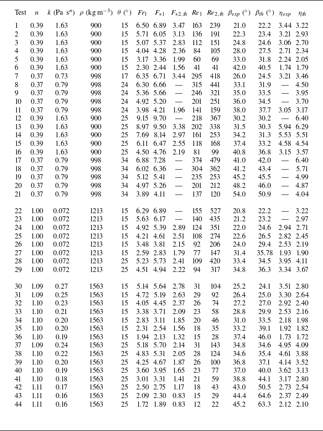


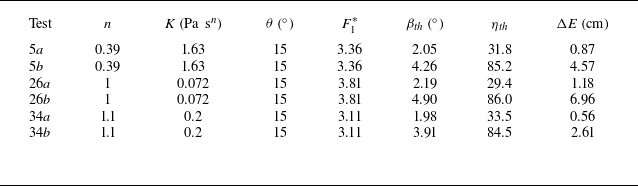


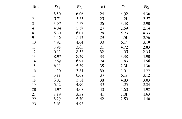


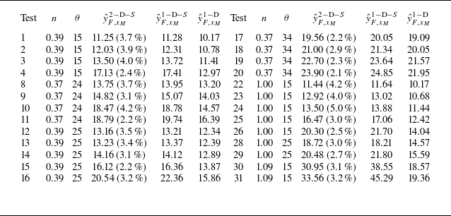


 Open access