





1. Introduction
Rotors and propellers are fundamental components in a broad array of modern engineering systems, from conventional aircraft propulsion units, wind turbines and, increasingly, unmanned aerial vehicles and electric vertical take-off and landing (eVTOL) vehicles for urban air mobility (UAM) (Ahuja et al. Reference Ahuja, Little, Majdalani and Hartfield2022; Pascioni et al. Reference Pascioni, Watts, Houston, Lind, Stephenson and Bain2022; Ko, German & Rauleder Reference Ko, German and Rauleder2023). The projected expansion of eVTOL operations holds promise for addressing urban congestion and facilitating sustainable aerial transport in densely populated cities, thereby accelerating research and certification activities. Yet community acceptance of these vehicles, which is tightly and critically coupled to noise, remains a concern (Torija & Clark Reference Torija and Clark2021; Rizzi & Rafaelof Reference Rizzi and Rafaelof2021; Yuan et al. Reference Yuan, Zachos, Langelaan, Greenwood and Brentner2024; Huang Reference Huang2025). Unlike high-altitude transport aircraft, UAM vehicles take off, land and hover near pedestrians, where both the absolute level and the qualitative character of the sound field govern perceived acceptability (Casagrande Hirono, Robertson & Torija Martinez Reference Casagrande Hirono, Robertson and Torija Martinez2024). This places renewed emphasis on physical understanding of propeller noise generation mechanisms, especially since the interaction between a propeller and turbulent inflow is often a dominant source of noise in eVTOL aircraft (Hall Reference Hall2017; Amargianitakis et al. Reference Amargianitakis, Self, Proenca, Torija Martinez and Synodinos2022; Little et al. Reference Little, Majdalani, Hartfield and Ahuja2022; Ahmed et al. Reference Ahmed, Zaman, Rezgui and Azarpeyvand2024). The environments in which these vehicles will operate feature a wide range of turbulent inflows generated by lifting or control surfaces, the fuselage, novel wing configurations and upstream or surrounding objects in urban landscapes, such as pylons, airframes, trees and even buildings (Casalino, van der Velden & Romani Reference Casalino, van der Velden and Romani2019). The present study aims to advance knowledge of turbulence ingestion noise mechanisms when turbulence with distinct characteristics (i.e. intensity, coherence and length scales) is ingested by the propeller, using numerical simulations.
This work primarily focuses on turbulence ingestion since it sets the structure of the unsteady loading that drives the sound field while operating in urban environments. Paterson & Amiet (Reference Paterson and Amiet1982) showed that turbulence ingestion is the dominant propeller noise mechanism at the moderate to high frequencies, which determine perceived noise levels. Amiet (Reference Amiet1975) framed this as a gust-response problem in which blades act as spatial samplers of convecting disturbances. In urban and installed contexts, these disturbances are rarely homogeneous or stationary; therefore, the ingestion pathway becomes central to prediction and control (Silva et al. Reference Silva, Johnson, Antcliff and Patterson2018). The practical importance is immediately evident for eVTOL operations, where wakes, shear layers and boundary layers are present near vertiports (Kellermann, Biehle & Fischer Reference Kellermann, Biehle and Fischer2020). Certification and community studies reinforce that the temporal regularity of the signature matters as much as the absolute level, which places ingestion at the centre of noise acceptability (Rizzi & Rafaelof Reference Rizzi and Rafaelof2021; Thai et al. Reference Thai, Bain, Josephson, Naru, Lympany and Page2025).
A number of aeroacoustic sources contribute to the propeller noise spectrum. Thickness and loading dipoles are primary in most regimes, with trailing-edge (TE) noise, tip–vortex interaction, turbulence interaction and installation effects shaping the tones at midfrequencies and the broadband components (Blake Reference Blake1986; Brooks, Pope & Marcolini Reference Brooks, Pope and Marcolini1989; Roger & Moreau Reference Roger and Moreau2010; Glegg & Devenport Reference Glegg and Devenport2024). At low altitude and in proximity to structures, the increment relative to isolated operations is frequently dominated by ingestion of turbulence (Casalino et al. Reference Casalino, van der Velden and Romani2019). As coherent or partially coherent structures convect through the propeller disk, they modulate sectional loading, and the far-field responds with distinctive patterns that depend on the scale and coherence of the ingested eddies (McAlpine, Powles & Tester Reference McAlpine, Powles and Tester2009; Schmitz Reference Schmitz2016; Grande et al. Reference Grande, Ragni, Avallone and Casalino2022; Shao, Chen & Huang Reference Shao, Chen and Huang2025). There are a number of classical models connecting surface sources (often in response to near-field turbulence) to far-field noise for both simple and complex geometries (Curle Reference Curle1955; Ffowcs Williams & Hawkings Reference Ffowcs Williams and Hawkings1969; Goldstein Reference Goldstein1976). Modern prediction strategies rely on acoustic analogies that map the unsteady surface loading to the far-field, and are widely applied in computational fluid dynamics flow solvers used to resolve unsteady loads in complex configurations (Ahuja et al. Reference Ahuja, Little, Majdalani and Hartfield2022; Lockard Reference Lockard2022; Zhang et al. Reference Zhang, Xiao, Liu and Chen2022).
A defining feature of turbulence ingestion noise is its sensitivity to the spatial and temporal characteristics of the incoming turbulence. Large-scale turbulence (LST), often generated by atmospheric disturbances, upstream obstacles or bluff-body wakes, contains coherent vortical structures with large integral scales. When ingested, these structures impose correlated unsteady loads across multiple blades, giving rise to the modulation of blade passing frequency (BPF) tones and the characteristic haystacking phenomenon in acoustic spectra (McAlpine et al. Reference McAlpine, Powles and Tester2009; Schmitz Reference Schmitz2016; Grande et al. Reference Grande, Ragni, Avallone and Casalino2022). In contrast, small-scale turbulence (SST), typically originating from shear-layer breakdown or wakes from smaller objects, generates relatively uncorrelated, high-frequency fluctuations. Small-scale turbulence ingestion is usually associated with broadband noise augmentation and suppression of tonal coherence (Rego et al. Reference Rego, Avallone, Ragni and Casalino2022; Zamponi et al. Reference Zamponi, Satcunanathan, Moreau, Meinke, Schröder and Schram2023; Jamaluddin et al. Reference Jamaluddin, Celik, Baskaran, Rezgui and Azarpeyvand2024). However, recent studies demonstrated that SST ingestion may also produce tonal features, particularly when the shed vortical structures retain coherence or interact strongly with the blade tip (Gonzalez-Martino et al. Reference Gonzalez-Martino, Romani, Wang and Casalino2018; Wu et al. Reference Wu, Jiang, Ma, Chen and Huang2022, Reference Wu, Li, Zhang, Zhong and Huang2024).
Several experimental and numerical studies have explored turbulence ingestion noise using controlled inflows. Paterson & Amiet (Reference Paterson and Amiet1982) used standard inflow models to correlate turbulence spectra of the inflow to rotor harmonic content and clarified how modulation at a secondary frequency appears as symmetric sidebands in the noise spectra. McAlpine et al. (Reference McAlpine, Powles and Tester2009) examined rotors exposed to turbulence with varied integral scales and reported a systematic broadening of the blade passing harmonics as the scale increased. They linked this trend to slowly varying envelopes of the carrier tones. Successive work by the same group introduced a weak-scattering framework that rationalises the observed humps around $\mathrm{BPF}$
and its harmonics and quantifies their sensitivity to inflow coherence (McAlpine & Tester Reference McAlpine and Tester2020). A particularly relevant contribution was provided by Wang, Wang & Wang (Reference Wang, Wang and Wang2021), who investigated the noise generated by a rotor ingesting the turbulent wake of a circular cylinder using LES coupled with Ffowcs Williams–Hawkings (FW-H). Their work revealed distinct spectral contributions associated with the cylinder vortex-shedding frequency and the blade-passing frequency. Importantly, they showed that the fluctuating wake is responsible for most of the rotor acoustic response, whereas the mean wake velocity deficit contributes strongly at the blade-passing frequency. They also reported relatively weak blade-to-blade correlations and source coherence, highlighting the importance of inflow organisation in determining the repeatability of the blade response. Cylinder wake ingestion by a propeller adds a distinct behaviour. Gonzalez-Martino et al. (Reference Gonzalez-Martino, Romani, Wang and Casalino2018) showed that periodic shedding can phase-lock to the rotor cadence and generate clean sidebands at
$\mathrm{BPF}$
and its harmonics and quantifies their sensitivity to inflow coherence (McAlpine & Tester Reference McAlpine and Tester2020). A particularly relevant contribution was provided by Wang, Wang & Wang (Reference Wang, Wang and Wang2021), who investigated the noise generated by a rotor ingesting the turbulent wake of a circular cylinder using LES coupled with Ffowcs Williams–Hawkings (FW-H). Their work revealed distinct spectral contributions associated with the cylinder vortex-shedding frequency and the blade-passing frequency. Importantly, they showed that the fluctuating wake is responsible for most of the rotor acoustic response, whereas the mean wake velocity deficit contributes strongly at the blade-passing frequency. They also reported relatively weak blade-to-blade correlations and source coherence, highlighting the importance of inflow organisation in determining the repeatability of the blade response. Cylinder wake ingestion by a propeller adds a distinct behaviour. Gonzalez-Martino et al. (Reference Gonzalez-Martino, Romani, Wang and Casalino2018) showed that periodic shedding can phase-lock to the rotor cadence and generate clean sidebands at $\mathrm{BPF}\pm f_0$
(where
$\mathrm{BPF}\pm f_0$
(where $f_0$
is the frequency of the periodic shedding), when coherence persists. This amplitude modulation has been previously described by Casalino, Jacob & Roger (Reference Casalino, Jacob and Roger2003), which was attributed to the spanwise modulation of the vortex shedding mechanism. Zhou, Wang & Wang (Reference Zhou, Wang and Wang2024) connected this dual response to neighbour-blade similarity and to the variability of the delay with which a structure is re-encountered across the span. Moreau et al. (Reference Moreau, Mendonca, Qazi, Prosser and Laurence2005) reviewed how these loading statistics propagate to sound and highlighted the role of compact sidebands in sustaining tonal prominence.
$f_0$
is the frequency of the periodic shedding), when coherence persists. This amplitude modulation has been previously described by Casalino, Jacob & Roger (Reference Casalino, Jacob and Roger2003), which was attributed to the spanwise modulation of the vortex shedding mechanism. Zhou, Wang & Wang (Reference Zhou, Wang and Wang2024) connected this dual response to neighbour-blade similarity and to the variability of the delay with which a structure is re-encountered across the span. Moreau et al. (Reference Moreau, Mendonca, Qazi, Prosser and Laurence2005) reviewed how these loading statistics propagate to sound and highlighted the role of compact sidebands in sustaining tonal prominence.
Wu et al. (Reference Wu, Jiang, Ma, Chen and Huang2022) confirmed with independent tests that small-scale wakes may still yield discrete modulation if phase memory is maintained over the blade-to-blade interval. Barbarino, Petrosino & Visingardi (Reference Barbarino, Petrosino and Visingardi2022) used high-fidelity numerical methods to show that upstream bodies modify the inflow coherence across the disk, which in turn modifies the tonal strength and directivity. Casalino et al. (Reference Casalino, Grande, Romani, Ragni and Avallone2021) used a lattice-Boltzmann approach to reproduce both broadband and tonal characteristics of installed propellers, providing insights into the installed propeller noise, which has also seen an increase in both components. Trascinelli et al. (Reference Trascinelli, Hanson, Romani, Casalino, Zhou, Zang and Azarpeyvand2024c ) computed SST ingestion on propellers and related sectional loading statistics to far-field spectra. Subsequently, they examined how changes to the ingested turbulence scale favour acoustic haystacking (Trascinelli et al. Reference Trascinelli, Hanson, Romani, Casalino, Zang, Zhou and Azarpeyvand2024a ).
The acoustic haystacking signature has been analysed from modelling and theory standpoints. Haystacking arises when energy contained in a tonal peak is spread to neighbouring frequencies when noise passes through a shear layer, resulting in spectral broadening of the tones (McAlpine & Tester Reference McAlpine and Tester2020). In the context of turbulence ingestion, it refers to the ‘hump’ grouping near the BPF tone and its harmonics resulting from the blade-to-blade correlation, where the same turbulent structure is cut multiple times by successive blades (Homicz & George Reference Homicz and George1974; Wisda et al. Reference Wisda, Alexander, Devenport and Glegg2014; Murray et al. Reference Murray, Devenport, Alexander, Glegg and Wisda2018; Hickling Reference Hickling2020). This produces a correlated unsteady blade loading and therefore broadband sound at the blade passage frequency and its harmonics (Molinaro et al. Reference Molinaro, Balantrapu, Hickling, Alexander, Devenport and Glegg2017). Sevik (Reference Sevik1974) observed this phenomenon, achieving good agreement between measurements and predictions except for haystacking humps at multiples of the BPF. Homicz & George (Reference Homicz and George1974) proposed a parameter to identify haystacking (i.e. tonal broadening), which related the time between blade passes to the convective time of a turbulent eddy through the rotor plane. It is given by $b\varOmega L/U_\infty \gg 1$
, where
$b\varOmega L/U_\infty \gg 1$
, where $b$
is the blade number,
$b$
is the blade number, $\varOmega$
is the angular velocity,
$\varOmega$
is the angular velocity, $L$
is the length scale and
$L$
is the length scale and $U_\infty$
is the free stream velocity. A value significantly larger than
$U_\infty$
is the free stream velocity. A value significantly larger than $1$
indicates an increased haystacking effect (Hickling et al. Reference Hickling, Balantrapu, Alexander, Millican, Devenport and Glegg2019). McAlpine et al. (Reference McAlpine, Powles and Tester2009) developed a weak-scattering concept in which broadband humps can arise from slow modulation of the carrier and showed how hump width scaled with envelope statistics. Raposo & Azarpeyvand (Reference Raposo and Azarpeyvand2024) extended this approach and demonstrated that inflow spectral shape, blade count and convective speed jointly determine whether sidebands remain compact or merge into a hump. Faria et al. (Reference Faria, Saab, Rodriguez and de Mattos Pimenta2020) proposed a practical methodology for installed propellers that quantifies amplitude modulation within a hybrid computational framework, enabling comparisons across inflow conditions. Huang (Reference Huang2023) provided an alternative interpretation through turbulence–cascade interactions and argued that haystacking reflects the spectral imprint of cascade response under inhomogeneous excitation. Zaman et al. (Reference Zaman, Falsi, Zang, Azarpeyvand and Camussi2024) performed a parametric experimental investigation on the far-field acoustic haystacking phenomenon for propeller boundary layer ingestion, characterising broadband hump appearance with the extent of boundary layer ‘emergence’, which showed good agreement with the parameter proposed by Homicz & George (Reference Homicz and George1974). Shao et al. (Reference Shao, Chen and Huang2025) formalised the idea that haystacking follows from the convolution of an inhomogeneous gust with a periodic sampling function representing blade cutting, and produced parametric predictions for hump amplitude and width that agree with high-fidelity simulations.
$1$
indicates an increased haystacking effect (Hickling et al. Reference Hickling, Balantrapu, Alexander, Millican, Devenport and Glegg2019). McAlpine et al. (Reference McAlpine, Powles and Tester2009) developed a weak-scattering concept in which broadband humps can arise from slow modulation of the carrier and showed how hump width scaled with envelope statistics. Raposo & Azarpeyvand (Reference Raposo and Azarpeyvand2024) extended this approach and demonstrated that inflow spectral shape, blade count and convective speed jointly determine whether sidebands remain compact or merge into a hump. Faria et al. (Reference Faria, Saab, Rodriguez and de Mattos Pimenta2020) proposed a practical methodology for installed propellers that quantifies amplitude modulation within a hybrid computational framework, enabling comparisons across inflow conditions. Huang (Reference Huang2023) provided an alternative interpretation through turbulence–cascade interactions and argued that haystacking reflects the spectral imprint of cascade response under inhomogeneous excitation. Zaman et al. (Reference Zaman, Falsi, Zang, Azarpeyvand and Camussi2024) performed a parametric experimental investigation on the far-field acoustic haystacking phenomenon for propeller boundary layer ingestion, characterising broadband hump appearance with the extent of boundary layer ‘emergence’, which showed good agreement with the parameter proposed by Homicz & George (Reference Homicz and George1974). Shao et al. (Reference Shao, Chen and Huang2025) formalised the idea that haystacking follows from the convolution of an inhomogeneous gust with a periodic sampling function representing blade cutting, and produced parametric predictions for hump amplitude and width that agree with high-fidelity simulations.
Global second-order tools, such as the spectral correlation-based modulation intensity distribution (MID) and its integrated form, remain informative to identify the extent of modulation in spectral content. Urbanek, Antoni & Barszcz (Reference Urbanek, Antoni and Barszcz2012) established the general framework of cyclostationary analysis for mechanical signals, and Grizewski et al. (Reference Grizewski, Behn, Funke and Siller2021) reviewed how integration bandwidth and frequency resolution can influence detection and bias. Bendat & Piersol (Reference Bendat and Piersol2010) formalised cross-correlation measures that can be adapted to blade-to-blade analysis, and subsequently Zhou et al. (Reference Zhou, Wang and Wang2024) linked amplitude similarity and spanwise delay to the collapse of carrier-conditioned coherence at the expected modulation frequency when large-scale ingestion dominates.
In addition, studies on shrouded propellers have shown how confinement alters both the turbulence entering the rotor and its acoustic signature (Go et al. Reference Go, Kingan, Bowen and Azarpeyvand2024). Studies of collective pitch effects (Quaroni et al. Reference Quaroni, Merino-Martinez, Monteiro and Kumar2024) and flow-control devices upstream of rotors (Teruna et al. Reference Teruna, Rego, Casalino, Ragni and Avallone2022) further suggest that careful management of inflow turbulence could serve as a viable noise mitigation strategy. These findings are particularly relevant for UAM applications, where propellers will often be mounted in proximity to lifting surfaces, ducts or fuselage components that shed unsteady wakes. Despite this body of work, controlled high-fidelity comparisons of propellers ingesting wake disturbances with distinct scale and coherence characteristics remain limited. Facility limitations constrain most experimental campaigns and rely on ambient or grid-generated turbulence, limiting reproducibility as well as the ability to control the turbulence energy spectra of the inflow (McAlpine et al. Reference McAlpine, Powles and Tester2009; Schmitz Reference Schmitz2016). As a result, predictive models for rotor acoustics in the context of UAM remain underdeveloped. Yet distinguishing the roles of turbulence scale and coherence is crucial, both for accurate noise prediction and for identifying strategies to reduce noise in urban operations.
The present study aims to address this gap by conducting numerical simulations using a lattice-Boltzmann-based solver to investigate the flow and noise characteristics arising from a two-bladed propeller ingesting two distinct turbulent wakes. The wake ‘inflows’ are generated from upstream cylinders of two distinct diameters: one generating coherent, LST (approximately of the order of the cylinder diameter), and the other producing smaller-scale turbulence. This arrangement allows a controlled comparison between two wake-ingestion cases generated by upstream cylinders of different diameters, thereby exposing the propeller to inflows with distinct scale, coherence, spatial extent and intensity under otherwise matched propeller operating conditions. This arrangement allows a controlled comparison between two wake-ingestion cases generated by upstream cylinders of different diameters, thereby exposing the propeller to inflows with distinct scale, coherence and spatial extent under otherwise identical operating conditions. Although the two cylinder wakes generate markedly different inflow conditions, several important parameters remain coupled, including turbulence intensity, spatial extent, wake coherence and the relative portion of the propeller disk exposed to the wake. In addition, other consequential quantities to propeller studies are not varied independently due to the limitations imposed and the extent of the analysis of numerical studies. The objective of the present paper is therefore to provide a high-fidelity mechanistic comparison between two canonical ingestion regimes, which can subsequently be used in predictive models. For clarity, throughout this work, SST and LST refer to ingested wake disturbances whose dominant spatial and temporal scales are, respectively, small and large relative to the blade chord and the blade-pass time. These labels, therefore, describe the characteristic organisation of the incoming unsteady wake, rather than homogeneous turbulence. In the present configuration, the SST ingestion case is associated with more compact and localised wake structures, whereas the LST ingestion case is associated with broader, more coherent wake disturbances that affect a larger portion of the propeller disk. Both conditions are representative of unique eVTOL configurations and operations, for example, wakes from slender upstream elements (e.g. struts or cables) that generate more compact high-frequency disturbances, or larger obstructions (e.g. pylons or fairings) that introduce lower-frequency, disk-wide inflow non-uniformity.
Using both time-averaged and phase-averaged analyses, the study examines how differences in inflow scale, coherence and spatial extent modify the sectional unsteady loading and the corresponding far-field noise. Furthermore, blade-level noise source decomposition and blade-to-blade correlation studies, coupled with modulation intensity analyses, help reveal two primary, yet distinct mechanisms in turbulence ingestion noise of a propeller in forward flight. The remainder of the paper is organised as follows. Section 2 describes the numerical framework and turbulence generation set-up. Section 3 is divided into § 3.1, which presents near-wake visualisation, cylinder wake characterisation, and blade loading analysis, and § 3.2, which presents far-field acoustic results, noise impact assessment, noise source decomposition and identification of haystacking noise. Finally, § 4 summarises the findings and outlines directions for future research.
2. Methodology
Given the low flow Mach number regime of interest in the present study, combining a flow solver based on the lattice-Boltzmann method (LBM) coupled with a very large-eddy simulation (VLES) turbulence model, with an acoustic analogy integral solver based on the impermeable surface integration of the FW-H equation (Ffowcs Williams & Hawkings Reference Ffowcs Williams and Hawkings1969) is well suited for the present study (Gonzalez-Martino et al. Reference Gonzalez-Martino, Romani, Wang and Casalino2018; Trascinelli et al. Reference Trascinelli, Hanson, Romani, Casalino, Zang, Zhou and Azarpeyvand2024a ). Therefore, surface data and near-field hydrodynamic solutions are computed via the inherently transient and scale-resolving LBM–VLES method, and then used to evaluate sound pressure signals in the far-field using the impermeable formulation of the FW-H analogy.
2.1. Numerical methods
This work utilises the numerical framework built using the LBM–VLES flow solver SIMULIA PowerFLOW to simulate the near- and far-field results of an isolated propeller, as well as SST and LST ingestion. The solver makes use of a computational mesh consisting of cubic lattices on a Cartesian grid, with each three-dimensional element referred to as a voxel. The LBM is inherently transient and provides dissipation/dispersion error characteristics similar to high-order finite difference computational aeroacoustic schemes (Marié et al. Reference Marié, Ricot and Sagaut2009). Therefore, this framework enables the resolution of unsteady flow fields and their acoustic emissions with high temporal and spatial fidelity, making it particularly well-suited for aeroacoustic studies involving rotor–turbulence interactions. The solver uses a discretised form of the Boltzmann equation on a uniform Cartesian mesh (Chen, Chen & Matthaeus Reference Chen, Chen and Matthaeus1992; Shan, Yuan & Chen Reference Shan, Yuan and Chen2006; Marié et al. Reference Marié, Ricot and Sagaut2009). The single-particle distribution function $f_i(\boldsymbol{x}, t)$
at location
$f_i(\boldsymbol{x}, t)$
at location $\boldsymbol{x}$
evolves according to the Bhatnagar–Gross–Krook approximation (Bhatnagar, Gross & Krook Reference Bhatnagar, Gross and Krook1954; Shan et al. Reference Shan, Yuan and Chen2006),
$\boldsymbol{x}$
evolves according to the Bhatnagar–Gross–Krook approximation (Bhatnagar, Gross & Krook Reference Bhatnagar, Gross and Krook1954; Shan et al. Reference Shan, Yuan and Chen2006),
 \begin{align} f_i(\boldsymbol{x} + \boldsymbol{c}_i \Delta t, t + \Delta t) = f_i(\boldsymbol{x}, t) - \frac {1}{\tau } \left ( f_i(\boldsymbol{x}, t) - f_i^{\textit{eq}}(\boldsymbol{x}, t) \right )\!, \end{align}
where $\boldsymbol{c}_i$
denotes the discrete lattice velocity in direction
$\boldsymbol{c}_i$
denotes the discrete lattice velocity in direction $i$
,
$i$
, $\tau$
is the relaxation time related to the kinematic viscosity
$\tau$
is the relaxation time related to the kinematic viscosity $\nu$
and
$\nu$
and $f_i^{\textit{eq}}$
is the equilibrium distribution function derived from the low-Mach expansion of the Maxwell–Boltzmann distribution,
$f_i^{\textit{eq}}$
is the equilibrium distribution function derived from the low-Mach expansion of the Maxwell–Boltzmann distribution,
 \begin{align} f_i^{\textit{eq}} = w_i \rho \left [ 1 + \frac {\boldsymbol{c}_i \boldsymbol{\cdot }\boldsymbol{u}}{c_s^2} + \frac {(\boldsymbol{c}_i \boldsymbol{\cdot }\boldsymbol{u})^2}{2 c_s^4} - \frac {\boldsymbol{u} \boldsymbol{\cdot }\boldsymbol{u}}{2 c_s^2} \right ], \end{align}
where $w_i$
are lattice-specific weights,
$w_i$
are lattice-specific weights, $\rho$
is the fluid density,
$\rho$
is the fluid density, $\boldsymbol{u}$
is the macroscopic velocity and
$\boldsymbol{u}$
is the macroscopic velocity and $c_s$
is the speed of sound on the lattice. Macroscopic flow variables, such as density and velocity, are recovered from the moments of the distribution function,
$c_s$
is the speed of sound on the lattice. Macroscopic flow variables, such as density and velocity, are recovered from the moments of the distribution function,
 \begin{align} \rho (\boldsymbol{x}, t) = \sum _i f_i(\boldsymbol{x}, t), \qquad \rho \boldsymbol{u}(\boldsymbol{x}, t) = \sum _i \boldsymbol{c}_i f_i(\boldsymbol{x}, t). \end{align}
Turbulence is modelled using a VLES approach, which consists of extending the Boussinesq approximation from a gas of particles to a gas of eddies. From a practical standpoint, this means calculating the relaxation time and the distribution function of the LBM collision operator by considering the turbulent kinetic energy and dissipation rate computed, at each voxel, by solving a $\mathrm{k}-\epsilon$
two-equation transport partial differential equation. A substantial difference between the LBM–VLES and RANS approaches consists in the fact that in LBM–VLES, Reynolds stresses are not directly modelled, but they are a consequence of the adaptation of the turbulent flow to a specific state of equilibrium. For the sake of the present study, the LBM–VLES hybrid approach ensures accurate resolution of both the ingestion of upstream turbulence and the associated propeller wake dynamics. As previously stated, the solver’s low dissipation and dispersion enable accurate solution of acoustic wave propagation (Hainaut et al. Reference Hainaut, Le Garrec, Polacsek, Mincu and Deck2018). Far-field acoustics are analysed through surface pressure data from all solid geometries using the impermeable formulation of the FW-H acoustic analogy (Ffowcs Williams & Hawkings Reference Ffowcs Williams and Hawkings1969) based on a forward-time solution of Farassat’s Formulation 1A (Farassat & Succi Reference Farassat and Succi1980; Casalino Reference Casalino2003). The formulation accounts for monopole and dipole noise associated with blade surface motion and pressure loading. Quadrupole sources have been taken into account using the permeable formulation of the FW-H analogy; however, they were considered negligible for propellers at low-tip Mach numbers (Casalino et al. Reference Casalino, Grande, Romani, Ragni and Avallone2021; Bu et al. Reference Bu, Wu, Bertin, Fang and Zhong2021).
$\mathrm{k}-\epsilon$
two-equation transport partial differential equation. A substantial difference between the LBM–VLES and RANS approaches consists in the fact that in LBM–VLES, Reynolds stresses are not directly modelled, but they are a consequence of the adaptation of the turbulent flow to a specific state of equilibrium. For the sake of the present study, the LBM–VLES hybrid approach ensures accurate resolution of both the ingestion of upstream turbulence and the associated propeller wake dynamics. As previously stated, the solver’s low dissipation and dispersion enable accurate solution of acoustic wave propagation (Hainaut et al. Reference Hainaut, Le Garrec, Polacsek, Mincu and Deck2018). Far-field acoustics are analysed through surface pressure data from all solid geometries using the impermeable formulation of the FW-H acoustic analogy (Ffowcs Williams & Hawkings Reference Ffowcs Williams and Hawkings1969) based on a forward-time solution of Farassat’s Formulation 1A (Farassat & Succi Reference Farassat and Succi1980; Casalino Reference Casalino2003). The formulation accounts for monopole and dipole noise associated with blade surface motion and pressure loading. Quadrupole sources have been taken into account using the permeable formulation of the FW-H analogy; however, they were considered negligible for propellers at low-tip Mach numbers (Casalino et al. Reference Casalino, Grande, Romani, Ragni and Avallone2021; Bu et al. Reference Bu, Wu, Bertin, Fang and Zhong2021).
The solver has been extensively validated for rotorcraft and propeller aeroacoustics, including configurations involving inflow turbulence, cylinder wake ingestion and installation effects (Gonzalez-Martino et al. Reference Gonzalez-Martino, Romani, Wang and Casalino2018; Teruna et al. Reference Teruna, Avallone, Casalino and Ragni2021; Romani et al. Reference Romani, Grande, Avallone, Ragni and Casalino2022; Salet, Casalino & Gonzalez-Martino Reference Salet, Casalino and Gonzalez-Martino2024; Trascinelli et al. Reference Trascinelli, Hanson, Lopes de Moraes Filho, Zang, Zhou and Azarpeyvand2024b ). Its suitability for low Mach number, unsteady aeroacoustics, with accurate near-field resolution, makes it appropriate for the present investigation, which focuses on scale-dependent turbulence ingestion noise mechanisms.
2.2. Numerical set-up
The study selected a Mejzlik 12ʹʹ × 12ʹʹ two-bladed ( $R={152.3}\,\mathrm{mm}$
) propeller, chosen due to its scalability for use in eVTOL vehicles (Cerny & Breitsamter Reference Cerny and Breitsamter2020), as well as being suitable for forward flight operations as tested by Hanson et al. (Reference Hanson, Baskaran, Pullin, Zhou, Zang and Azarpeyvand2022) in experimental campaigns. For all cases, the propeller was operated at a constant rotational speed of 8000 r.p.m. with an inflow velocity of
$R={152.3}\,\mathrm{mm}$
) propeller, chosen due to its scalability for use in eVTOL vehicles (Cerny & Breitsamter Reference Cerny and Breitsamter2020), as well as being suitable for forward flight operations as tested by Hanson et al. (Reference Hanson, Baskaran, Pullin, Zhou, Zang and Azarpeyvand2022) in experimental campaigns. For all cases, the propeller was operated at a constant rotational speed of 8000 r.p.m. with an inflow velocity of $U_{\infty }={14}\,\mathrm{ms^{-1}}$
. The blade operating parameters can be summarised by its maximum chord of
$U_{\infty }={14}\,\mathrm{ms^{-1}}$
. The blade operating parameters can be summarised by its maximum chord of $c_{\mathit{max}} = {22.13}\,\mathrm{mm}$
, the corresponding maximum chord Reynolds number is
$c_{\mathit{max}} = {22.13}\,\mathrm{mm}$
, the corresponding maximum chord Reynolds number is ${1.89 \times 10^5}{}$
, and the tip Mach number is
${1.89 \times 10^5}{}$
, and the tip Mach number is $M_{\mathit{tip}} =0.372$
, placing the present configuration in the low-Mach-number regime for propeller studies. For propellers operating in forward flight with free stream velocity
$M_{\mathit{tip}} =0.372$
, placing the present configuration in the low-Mach-number regime for propeller studies. For propellers operating in forward flight with free stream velocity $U_{\infty }$
, the advance ratio
$U_{\infty }$
, the advance ratio $J$
is defined by
$J$
is defined by
 \begin{align} J=\frac {U_{\infty }}{nD}, \end{align}
which gives a value $J = 0.35$
for the present cases. The simulation framework was developed using the multicopter aero and acoustic simulations (MAAS) workflow (Casalino et al. Reference Casalino, van der Velden and Romani2019; van der Velden, Romani & Casalino Reference van der Velden, Romani and Casalino2021) and subsequently adjusted to include the cylinders and necessary refinement regions. The side view for the ingestion cases is shown in figure 1(a). In realistic eVTOL configurations, wakes shed by nearby upstream elements may produce an asymmetric loading response. The cylinder is vertically offset by
$J = 0.35$
for the present cases. The simulation framework was developed using the multicopter aero and acoustic simulations (MAAS) workflow (Casalino et al. Reference Casalino, van der Velden and Romani2019; van der Velden, Romani & Casalino Reference van der Velden, Romani and Casalino2021) and subsequently adjusted to include the cylinders and necessary refinement regions. The side view for the ingestion cases is shown in figure 1(a). In realistic eVTOL configurations, wakes shed by nearby upstream elements may produce an asymmetric loading response. The cylinder is vertically offset by $y = 0.5R$
from the rotational axis of the propeller and placed at a distance
$y = 0.5R$
from the rotational axis of the propeller and placed at a distance $l$
upstream of the plane of rotation. This offset was selected to generate a representative partial-disk ingestion condition, consistent with experimentally investigated installed-propeller configurations relevant to eVTOL applications (Hanson Reference Hanson2025), which revealed this offset as having the most significant interaction noise. The present work, therefore, adopts this offset as a representative case rather than treating it as an independently varied design parameter. The small cylinder with a diameter of
$l$
upstream of the plane of rotation. This offset was selected to generate a representative partial-disk ingestion condition, consistent with experimentally investigated installed-propeller configurations relevant to eVTOL applications (Hanson Reference Hanson2025), which revealed this offset as having the most significant interaction noise. The present work, therefore, adopts this offset as a representative case rather than treating it as an independently varied design parameter. The small cylinder with a diameter of $d_{\mathit{S}}={22.25}\,\mathrm{mm}$
was placed at
$d_{\mathit{S}}={22.25}\,\mathrm{mm}$
was placed at $l = 5d_{\mathit{S}}$
to produce small-scale turbulent structures, while a larger cylinder with a diameter
$l = 5d_{\mathit{S}}$
to produce small-scale turbulent structures, while a larger cylinder with a diameter $d_{\mathit{L}}={101.6}\,\mathrm{mm}$
was placed at
$d_{\mathit{L}}={101.6}\,\mathrm{mm}$
was placed at $l = 5d_{\mathit{L}}$
to produce large-scale turbulent structures. The inflow seen by the propeller therefore contains both coherent wake organisation and stochastic fluctuations, with the coherent component being more dominant in the LST ingestion case. This distinction is important for interpreting the resulting loading and acoustic response. Figure 1(b) shows the front view of the turbulence ingestion case propeller disk with the relative position of the cylinder and the angular blade position denoted by
$l = 5d_{\mathit{L}}$
to produce large-scale turbulent structures. The inflow seen by the propeller therefore contains both coherent wake organisation and stochastic fluctuations, with the coherent component being more dominant in the LST ingestion case. This distinction is important for interpreting the resulting loading and acoustic response. Figure 1(b) shows the front view of the turbulence ingestion case propeller disk with the relative position of the cylinder and the angular blade position denoted by $\psi$
.
$\psi$
.
Schematic of the numerical set-up: (a) side view of the turbulence ingestion cases with far-field microphone array $\theta$
, and (b) front view of the turbulence ingestion case with azimuthal propeller rotation angle
$\theta$
, and (b) front view of the turbulence ingestion case with azimuthal propeller rotation angle $\psi$
and direction of rotation. Diagram not to scale.
$\psi$
and direction of rotation. Diagram not to scale.

Variable resolution regions for the ingestion case showing (a) boundary layer regions and (b–d) wake regions.

Variable resolution 15 (blue) showing the near-field resolution along the propeller blade.

Figure 2 shows the voxel distribution regions for the ingestion set-up. The isolated case retains the same near-field regions, excluding the cylinder wake regions. The spatial resolution is controlled using variable resolution (VR) regions defined in proximity to the propeller as geometry offsets, and as far-field flow regions. The minimum voxel size was selected to maintain approximately $200$
cells per mean blade chord in the near-blade region and is found in the highest VR region (VR 15). This value is indicative of the fine-resolution cases, resulting in
$200$
cells per mean blade chord in the near-blade region and is found in the highest VR region (VR 15). This value is indicative of the fine-resolution cases, resulting in $y^+\leqslant 5$
over the blade surface. The near-field resolution along the propeller blade is shown in figure 3. For the ingestion cases, the
$y^+\leqslant 5$
over the blade surface. The near-field resolution along the propeller blade is shown in figure 3. For the ingestion cases, the $y^+$
on the cylinder surface was kept at approximately
$y^+$
on the cylinder surface was kept at approximately $10$
to ensure the correct boundary-layer separation point. This was evaluated in previous studies which utilised a similar VR region distribution and set-up (Trascinelli et al. Reference Trascinelli, Hanson, Romani, Casalino, Zang, Zhou and Azarpeyvand2024a
,
Reference Trascinelli, Hanson, Romani, Casalino, Zhou, Zang and Azarpeyvandc
). The fine-equivalent voxel counts for the isolated, SST ingestion and LST ingestion cases are
$10$
to ensure the correct boundary-layer separation point. This was evaluated in previous studies which utilised a similar VR region distribution and set-up (Trascinelli et al. Reference Trascinelli, Hanson, Romani, Casalino, Zang, Zhou and Azarpeyvand2024a
,
Reference Trascinelli, Hanson, Romani, Casalino, Zhou, Zang and Azarpeyvandc
). The fine-equivalent voxel counts for the isolated, SST ingestion and LST ingestion cases are $25\times10^6$
,
$25\times10^6$
, $67\times10^6$
and
$67\times10^6$
and $47\times10^6$
, respectively. Whilst maintaining
$47\times10^6$
, respectively. Whilst maintaining $y^+\leqslant 30$
to ensure the correct activation of the wall model, the cylinder shedding and far-field results were again comparable to the fine-resolution case results presented here. The remainder of the VR regions are arranged as concentric spheres centred around the propeller’s origin. Far-field boundary conditions are prescribed as a pressure and velocity inlet at the surface of a sphere of
$y^+\leqslant 30$
to ensure the correct activation of the wall model, the cylinder shedding and far-field results were again comparable to the fine-resolution case results presented here. The remainder of the VR regions are arranged as concentric spheres centred around the propeller’s origin. Far-field boundary conditions are prescribed as a pressure and velocity inlet at the surface of a sphere of $800R$
, where
$800R$
, where $R$
is the propeller radius. To avoid reflections from the boundary condition surface, an acoustic sponge layer is introduced in the domain, which consists of a sphere of radius
$R$
is the propeller radius. To avoid reflections from the boundary condition surface, an acoustic sponge layer is introduced in the domain, which consists of a sphere of radius $400R$
centred on the propeller. This region acts as a damper for acoustic waves and reflections by progressively increasing the kinematic viscosity from its initial physical magnitude to an artificial value (Romani et al. Reference Romani, Grande, Avallone, Ragni and Casalino2022). The far-field analysis is conducted using surface pressure fluctuations extracted from the solid surfaces (cylinder included) of the simulation. These are sampled at a frequency of
$400R$
centred on the propeller. This region acts as a damper for acoustic waves and reflections by progressively increasing the kinematic viscosity from its initial physical magnitude to an artificial value (Romani et al. Reference Romani, Grande, Avallone, Ragni and Casalino2022). The far-field analysis is conducted using surface pressure fluctuations extracted from the solid surfaces (cylinder included) of the simulation. These are sampled at a frequency of ${2\times 10^5}\,\mathrm{Hz}$
at each surface element, or surfel, for all solid surfaces. The cylinders retain the side plates used in the experiments to ensure the correct development of the wake, without significant contribution from the finite-span effect of the cylinder. The simulation comprises
${2\times 10^5}\,\mathrm{Hz}$
at each surface element, or surfel, for all solid surfaces. The cylinders retain the side plates used in the experiments to ensure the correct development of the wake, without significant contribution from the finite-span effect of the cylinder. The simulation comprises ${0.3}\,\mathrm{s}$
of physical time, corresponding to 40 propeller revolutions. A sliding mesh, in combination with a rotating local reference frame, allows for the rotation of both the propeller and the spinner.
${0.3}\,\mathrm{s}$
of physical time, corresponding to 40 propeller revolutions. A sliding mesh, in combination with a rotating local reference frame, allows for the rotation of both the propeller and the spinner.
2.3. Validation study
Validation of both the isolated cylinders and the propeller simulations is presented in this section to provide confidence in the numerical solver used in this study, as well as the chosen mesh, resolution and set-up. The numerical results are compared with experimental results obtained from literature or from the Wind Tunnel facility at the University of Bristol.
2.3.1. Cylinder wake characterisation
Flow over a cylinder is one of the most well-documented cases, both numerically and experimentally, and has been summarised by Norberg (Reference Norberg2003). It is essential to validate the isolated cylinder simulation against experimental data to assess the solver’s ability to reproduce the cylinder’s shedding before using it to generate turbulence for ingestion cases. In order to simplify the non-dimensionalisation of values extracted from the numerical simulations, the cylinder diameter for both cylinders is denoted by $d=d_{\mathit{S}},\,d_{\mathit{L}}$
. As outlined in § 2.2, the two cylinders are immersed in a free stream velocity of
$d=d_{\mathit{S}},\,d_{\mathit{L}}$
. As outlined in § 2.2, the two cylinders are immersed in a free stream velocity of $U_\infty ={14}\,\mathrm{ms^{-1}}$
, to replicate the experimental campaign of an isolated cylinder by Hanson, Zang & Azarpeyvand (Reference Hanson, Zang and Azarpeyvand2024). The
$U_\infty ={14}\,\mathrm{ms^{-1}}$
, to replicate the experimental campaign of an isolated cylinder by Hanson, Zang & Azarpeyvand (Reference Hanson, Zang and Azarpeyvand2024). The $C_p$
distribution extracted from the isolated simulations indicates the solver predicts the correct surface pressure and transition point, consistent with the literature for similar Reynolds Numbers (Norberg Reference Norberg2003; Moussaed et al. Reference Moussaed, Wornom, Salvetti, Koobus and Dervieux2014; Chen, Zang & Azarpeyvand Reference Chen, Zang and Azarpeyvand2023) (see Appendix A).
$C_p$
distribution extracted from the isolated simulations indicates the solver predicts the correct surface pressure and transition point, consistent with the literature for similar Reynolds Numbers (Norberg Reference Norberg2003; Moussaed et al. Reference Moussaed, Wornom, Salvetti, Koobus and Dervieux2014; Chen, Zang & Azarpeyvand Reference Chen, Zang and Azarpeyvand2023) (see Appendix A).
The normalised mean streamwise velocity profiles in the wake of the isolated cylinders are shown in figure 4 and compared with the experimental measurements of Maryami et al. (Reference Maryami, Showkat Ali, Azarpeyvand and Afshari2020) at a similar Reynolds number. The profiles are extracted at four streamwise stations, (a) $x/d=0.5$
, (b) 1.5, (c) 3 and (d) 5, in order to assess the near-wake development up to the location of the ingestion plane. Overall, the numerical results reproduce the features of the wake evolution with good agreement. The strong velocity deficit close to the cylinder is captured, and the subsequent recovery and broadening of the wake with downstream distance are also predicted correctly. Small discrepancies are visible in the near wake, where the profile shape is particularly sensitive to the exact separation location; however, these differences progressively reduce downstream. Most importantly, at
$x/d=0.5$
, (b) 1.5, (c) 3 and (d) 5, in order to assess the near-wake development up to the location of the ingestion plane. Overall, the numerical results reproduce the features of the wake evolution with good agreement. The strong velocity deficit close to the cylinder is captured, and the subsequent recovery and broadening of the wake with downstream distance are also predicted correctly. Small discrepancies are visible in the near wake, where the profile shape is particularly sensitive to the exact separation location; however, these differences progressively reduce downstream. Most importantly, at $x/d=5$
, which is the relevant location for the ingestion cases studied in this paper, the numerical and experimental profiles are in satisfactory agreement, indicating that the solver captures the correct convection and diffusion of the cylinder wake before its interaction with the propeller. This provides confidence that the incoming velocity deficit and wake thickness imposed on the propeller in the turbulence-ingestion cases are physically representative.
$x/d=5$
, which is the relevant location for the ingestion cases studied in this paper, the numerical and experimental profiles are in satisfactory agreement, indicating that the solver captures the correct convection and diffusion of the cylinder wake before its interaction with the propeller. This provides confidence that the incoming velocity deficit and wake thickness imposed on the propeller in the turbulence-ingestion cases are physically representative.
Normalised streamwise velocity $u/U_\infty$
taken in the wake of the cylinder at four stations (
$u/U_\infty$
taken in the wake of the cylinder at four stations ( $x/d=0.5, \,1.5, \,3, \,5$
) with comparison with experimental results from Maryami et al. (Reference Maryami, Showkat Ali, Azarpeyvand and Afshari2020).
$x/d=0.5, \,1.5, \,3, \,5$
) with comparison with experimental results from Maryami et al. (Reference Maryami, Showkat Ali, Azarpeyvand and Afshari2020).

Figure 5 presents the normalised power spectral density of the three velocity fluctuation components extracted at $x/d=5$
downstream of the isolated cylinders. For both the SST and LST isolated cases, the spectra exhibit the expected broadband decay. The crosswise velocity component,
$x/d=5$
downstream of the isolated cylinders. For both the SST and LST isolated cases, the spectra exhibit the expected broadband decay. The crosswise velocity component, $\phi _{vv}$
, contains a narrowband peak at
$\phi _{vv}$
, contains a narrowband peak at $fd/U_\infty \approx 0.2$
, associated with the periodic shedding and consistent with the Strouhal number of the cylinders. This component exhibits the most pronounced peak because the cylinder wake is dominated by alternating cross-flow motion induced by the shedding process. The streamwise and spanwise components,
$fd/U_\infty \approx 0.2$
, associated with the periodic shedding and consistent with the Strouhal number of the cylinders. This component exhibits the most pronounced peak because the cylinder wake is dominated by alternating cross-flow motion induced by the shedding process. The streamwise and spanwise components, $\phi _{uu}$
and
$\phi _{uu}$
and $\phi _{ww}$
, display lower spectral levels but retain the same characteristic shedding signature, indicating that the unsteady wake dynamics are captured consistently across all three velocity components. The slope in the midfrequency range is also in reasonable agreement with the expected decay of turbulent wake spectra, comparable to the decay slope of
$\phi _{ww}$
, display lower spectral levels but retain the same characteristic shedding signature, indicating that the unsteady wake dynamics are captured consistently across all three velocity components. The slope in the midfrequency range is also in reasonable agreement with the expected decay of turbulent wake spectra, comparable to the decay slope of $f^{-5/3}$
, further supporting that the numerical resolution is sufficient to represent the energy scales of the cylinder wake relevant to the ingestion problem studied in the remainder of the paper. As a final verification, the fluctuating lift coefficient of the isolated cylinders was analysed to confirm that the shedding frequency is predicted correctly. Using the peak-to-peak spacing over multiple oscillation cycles, the corresponding Strouhal number was found to be
$f^{-5/3}$
, further supporting that the numerical resolution is sufficient to represent the energy scales of the cylinder wake relevant to the ingestion problem studied in the remainder of the paper. As a final verification, the fluctuating lift coefficient of the isolated cylinders was analysed to confirm that the shedding frequency is predicted correctly. Using the peak-to-peak spacing over multiple oscillation cycles, the corresponding Strouhal number was found to be $St = 0.196$
, which is in close agreement with the canonical value expected for subcritical circular-cylinder shedding. This is also consistent with the distinct spectral peak observed in figure 5(b), confirming that the mesh resolution is sufficient to capture the dominant wake unsteadiness.
$St = 0.196$
, which is in close agreement with the canonical value expected for subcritical circular-cylinder shedding. This is also consistent with the distinct spectral peak observed in figure 5(b), confirming that the mesh resolution is sufficient to capture the dominant wake unsteadiness.
Normalised power spectral density of the velocity fluctuations of the (a) streamwise, $\phi _{uu}$
, (b) crosswise,
$\phi _{uu}$
, (b) crosswise, $\phi _{vv}$
, and (c) spanwise,
$\phi _{vv}$
, and (c) spanwise, $\phi _{ww}$
, components for the isolated cylinders taken at
$\phi _{ww}$
, components for the isolated cylinders taken at $x/d=5$
.
$x/d=5$
.

Figure 5. Long description
Three line graphs depict the normalized power spectral density of velocity fluctuations for isolated cylinders. Panel A: The line graph shows the streamwise component. The x-axis is labeled fd/U infinity and ranges from 10^-1 to 10^1. The y-axis is labeled phi uu/(U infinity*d) and ranges from 10^0 to 10^-2. The red line represents the isolated SST cylinder, and the blue line represents the isolated LST cylinder. Both lines show a decreasing trend with some fluctuations. Panel B: The line graph shows the crosswise component. The x-axis is labeled fd/U infinity and ranges from 10^-1 to 10^1. The y-axis is labeled phi vv/(U infinity*d) and ranges from 10^0 to 10^-2. The red line represents the isolated SST cylinder, and the blue line represents the isolated LST cylinder. Both lines show a decreasing trend with some fluctuations. Panel C: The line graph shows the spanwise component. The x-axis is labeled fd/U infinity and ranges from 10^-1 to 10^1. The y-axis is labeled phi ww/(U infinity*d) and ranges from 10^0 to 10^-2. The red line represents the isolated SST cylinder, and the blue line represents the isolated LST cylinder. Both lines show a decreasing trend with some fluctuations. A dashed line with a slope of f^-5/3 is present in all panels.
2.3.2. Experimental propeller validation
Previous studies by Trascinelli et al. (Reference Trascinelli, Hanson, Romani, Casalino, Zhou, Zang and Azarpeyvand2024c
) presented results for cylinder-induced turbulence ingestion in forward-flight propellers, while Trascinelli et al. (Reference Trascinelli, Romani, Hanson, Casalino, Zang, Zhou and Azarpeyvand2025) focused on the large-scale ingestion case. The present manuscript extends beyond these earlier works by providing a comparative study of both SST and LST ingestion, together with additional validation, blade-level source decomposition and modulation-based analysis of the distinct aeroacoustic mechanisms. The isolated, SST and LST ingestion cases have been separately run, and the results validated against the experimental campaign, which mirrors this set-up. A mesh convergence study was performed to evaluate the accuracy of the solver in both performance and far-field noise. For brevity, only the LST ingestion case is presented, as it is the case with the larger physical cylinder–propeller gap and therefore more sensitive to grid refinement. A coarse, medium and fine mesh simulation was run, corresponding to a voxel count of $6.6 \times 10^7$
,
$6.6 \times 10^7$
, $1.22 \times 10^8$
and
$1.22 \times 10^8$
and $2.40 \times 10^8$
, with a
$2.40 \times 10^8$
, with a $y^+$
on the cylinder of
$y^+$
on the cylinder of ${\lt }\, 30$
,
${\lt }\, 30$
, ${\lt }\, 20$
and
${\lt }\, 20$
and ${\lt }\, 10$
, respectively. The non-dimensional thrust coefficient (
${\lt }\, 10$
, respectively. The non-dimensional thrust coefficient ( $C_T$
) and power coefficient (
$C_T$
) and power coefficient ( $C_P$
) are defined using the following equations:
$C_P$
) are defined using the following equations:
 \begin{align} C_{T} = \frac {T}{\rho n_r^{2} D^{4}},\qquad C_{P} = \frac {P}{\rho n_r^{3} D^{5}}, \end{align}
where $P = 2 \pi n_r Q$
. Here,
$P = 2 \pi n_r Q$
. Here, $T$
and
$T$
and $Q$
are the thrust force and torque produced by the propeller,
$Q$
are the thrust force and torque produced by the propeller, $\rho$
is the density of air and
$\rho$
is the density of air and $n_r$
is the propeller rotational rate measured in revolutions per second. The results presented in table 1 demonstrate convergence, with mesh independence achieved at the medium resolution. The slight increase in
$n_r$
is the propeller rotational rate measured in revolutions per second. The results presented in table 1 demonstrate convergence, with mesh independence achieved at the medium resolution. The slight increase in $C_P$
with mesh refinement is attributed to improved resolution along the propeller blades, enabling more accurate capture of turbulence impingement.
$C_P$
with mesh refinement is attributed to improved resolution along the propeller blades, enabling more accurate capture of turbulence impingement.
Comparison of thrust and power coefficients with experimental results and numerical mesh refinement campaign for the LST case.

Table 1. Long description
A table comparing thrust and power coefficients across different simulation resolutions and experimental results. The table has four rows and three columns. The columns are labeled ‘Case’, ‘C_T [-]’, and ‘C_P [-]’. The rows are labeled ‘Experiment’, ‘Simulation - coarse’, ‘Simulation - medium’, and ‘Simulation - fine’. Row 1: Experiment, C_T [-], 0.0939, C_P [-], 0.0703. Row 2: Simulation - coarse, C_T [-], 0.0930, C_P [-], 0.0642. Row 3: Simulation - medium, C_T [-], 0.0931, C_P [-], 0.0640. Row 4: Simulation - fine, C_T [-], 0.0932, C_P [-], 0.0640.
The computed thrust coefficient agreed with the experimental results within 1 %, whereas the power coefficient was underpredicted by approximately 9 %. This discrepancy is attributed to sensitivity to viscous and near-wall modelling, as well as to experimental uncertainties arising from blade surface imbalances and torque measurements. Nevertheless, the close match in force coefficients provides confidence in the numerical results for further analysis.
Comparison of numerical and experimental results extracted from the far-field microphone located at $\theta =60^\circ$
for (a,b) isolated propeller, (c,d) SST ingestion and (e,f) LST ingestion with zoomed-in view around the first BPF.
$\theta =60^\circ$
for (a,b) isolated propeller, (c,d) SST ingestion and (e,f) LST ingestion with zoomed-in view around the first BPF.

Figure 6. Long description
The image contains six line graphs comparing numerical and experimental results for different propeller conditions. Panel A and B show results for an isolated propeller, Panel C and D for SST ingestion, and Panel E and F for LST ingestion. Each pair includes a zoomed-in view around the first BPF. The x-axis represents the frequency ratio (f/BPF) ranging from 0 to 50, and the y-axis represents the sound pressure level (SPL) in decibels (dB) ranging from 30 to 75. The black lines represent measurements, while the gray lines represent PowerFLOW predictions. Panel A shows a peak around 1.0 on the x-axis with SPL values reaching around 75 dB. Panel B provides a zoomed-in view of this peak. Panel C shows a similar peak around 1.0 with SPL values also reaching around 75 dB, and Panel D provides a zoomed-in view. Panel E shows a broader peak around 1.0 with SPL values reaching around 70 dB, and Panel F provides a zoomed-in view. The graphs illustrate the comparison between numerical predictions and experimental measurements for different propeller conditions, highlighting the accuracy of the PowerFLOW model in predicting sound pressure levels.
Far-field noise analysis using the impermeable formulation of the FW-H analogy predicted the correct magnitude of blade-pass-frequency tones and broadband levels as shown in figure 6. A comparison with the permeable formulation of the FW-H analogy showed good overall spectral agreement with the impermeable formulation over the dominant BPF range; however, because the permeable control surface is sampled in a coarser VR region and is therefore subject to a lower Nyquist frequency, the impermeable formulation was retained for the remainder of the paper. The data were extracted and compared for all experimental microphone locations; however, only the microphone at $\theta =60^\circ$
is presented for brevity. In addition, the mesh refinement study discussed above has also demonstrated the correct cylinder shedding and convergence of far-field results towards the
$\theta =60^\circ$
is presented for brevity. In addition, the mesh refinement study discussed above has also demonstrated the correct cylinder shedding and convergence of far-field results towards the $y^+$
value used and presented in this study. The isolated case captures the tonal peaks at the BPF and its harmonics, typical for a propeller. Differences between the numerical and experimental results are most pronounced in the low-frequency range of the spectra (BPF
$y^+$
value used and presented in this study. The isolated case captures the tonal peaks at the BPF and its harmonics, typical for a propeller. Differences between the numerical and experimental results are most pronounced in the low-frequency range of the spectra (BPF ${\lt }\, 2$
for the isolated and the SST ingestion case and BPF
${\lt }\, 2$
for the isolated and the SST ingestion case and BPF ${\lt } \,1$
for the LST ingestion case), where the discrepancies can be substantial. These differences are largely attributed to background noise contamination in the experimental facility (see Appendix A), as well as to the absence of motor and shaft contributions in the numerical model (Trascinelli et al. Reference Trascinelli, Romani, Hanson, Casalino, Zang, Zhou and Azarpeyvand2025). Shaft tones at half-integers of the BPF and its harmonics are also observed in the experiments, but are not present in the numerical simulation since no motor and shaft were included.
${\lt } \,1$
for the LST ingestion case), where the discrepancies can be substantial. These differences are largely attributed to background noise contamination in the experimental facility (see Appendix A), as well as to the absence of motor and shaft contributions in the numerical model (Trascinelli et al. Reference Trascinelli, Romani, Hanson, Casalino, Zang, Zhou and Azarpeyvand2025). Shaft tones at half-integers of the BPF and its harmonics are also observed in the experiments, but are not present in the numerical simulation since no motor and shaft were included.
Similar to the isolated case, both the SST and LST ingestion cases are able to capture the tonal peaks at the BPF and its harmonics, with the amplitudes in good agreement with the experiments. In addition, the SST ingestion simulation shows a distinct vortex-shedding peak at $0.5\mathrm{BPF}$
, consistent with the literature, as well as the midfrequency range, which is dominated by the integer and half-integer multiples of the BPF harmonics. In contrast, the LST ingestion case displays distinct side-peaks around the tones (i.e. BPF and its harmonics), most visible at the BPF. Moreover, clear spectral broadening and some minor ‘blue-shifts’ can also be observed at the harmonics of the BPF, characteristics of the haystacking phenomenon (Murray et al. Reference Murray, Devenport, Alexander, Glegg and Wisda2018; McAlpine & Tester Reference McAlpine and Tester2020; Huang Reference Huang2023). Moreover, the broadband noise components are predicted correctly when compared with the experiments, keeping spectral and overall sound pressure level (OASPL) errors within
$0.5\mathrm{BPF}$
, consistent with the literature, as well as the midfrequency range, which is dominated by the integer and half-integer multiples of the BPF harmonics. In contrast, the LST ingestion case displays distinct side-peaks around the tones (i.e. BPF and its harmonics), most visible at the BPF. Moreover, clear spectral broadening and some minor ‘blue-shifts’ can also be observed at the harmonics of the BPF, characteristics of the haystacking phenomenon (Murray et al. Reference Murray, Devenport, Alexander, Glegg and Wisda2018; McAlpine & Tester Reference McAlpine and Tester2020; Huang Reference Huang2023). Moreover, the broadband noise components are predicted correctly when compared with the experiments, keeping spectral and overall sound pressure level (OASPL) errors within ${2}{-}{4}\,\mathrm{dB}$
. More importantly, it is useful to highlight that the acoustic spectra of both configurations appears to exhibit amplitude modulation between the propeller and the cylinder, which can be identified as
${2}{-}{4}\,\mathrm{dB}$
. More importantly, it is useful to highlight that the acoustic spectra of both configurations appears to exhibit amplitude modulation between the propeller and the cylinder, which can be identified as $m\text{BPF}\pm nf_0$
, where
$m\text{BPF}\pm nf_0$
, where $m,\,n = 1,\,2,\,3,\,\ldots$
and
$m,\,n = 1,\,2,\,3,\,\ldots$
and $f_0$
is the shedding frequency of the respective cylinder. Based on the numerical cylinder and experimental data validation study presented, LBM–VLES is deemed adequate for rotor–turbulence-ingestion noise studies. It should be carefully remarked that for the present simulations, the primary validation focuses on the noise spectra of the turbulence ingestion cases, accompanied by comparison of the aerodynamic forces from simulations with different voxel resolutions. Additional comparison on the wake velocity spectra of the cylinders from different voxel resolutions as well as with experimental measurements may shed further light on the differences in the acoustic spectra at low frequencies, which can further strengthen the validation. However, the comparison was not undertaken here due to resource constraints.
$f_0$
is the shedding frequency of the respective cylinder. Based on the numerical cylinder and experimental data validation study presented, LBM–VLES is deemed adequate for rotor–turbulence-ingestion noise studies. It should be carefully remarked that for the present simulations, the primary validation focuses on the noise spectra of the turbulence ingestion cases, accompanied by comparison of the aerodynamic forces from simulations with different voxel resolutions. Additional comparison on the wake velocity spectra of the cylinders from different voxel resolutions as well as with experimental measurements may shed further light on the differences in the acoustic spectra at low frequencies, which can further strengthen the validation. However, the comparison was not undertaken here due to resource constraints.
3. Results and discussion
3.1. Aerodynamic characteristics of turbulence ingestion
In order to understand the physical mechanisms of turbulence ingestion noise when a propeller is subjected to turbulent inflows of distinct characteristics, i.e. ingestion of SST and LST, a comprehensive examination of the near-field flow must be conducted and subsequently, correlating the flow features to the far-field acoustics. In this section, the flow and turbulence characteristics will first be presented.
Flow field visualisation of the (a–c) normalised mean root-mean-square (r.m.s.) of axial velocity component, $\bar {u}_{\mathit{rms}}/U_\infty$
, and (d–f) normalised mean spanwise vorticity,
$\bar {u}_{\mathit{rms}}/U_\infty$
, and (d–f) normalised mean spanwise vorticity, $\bar {\omega }_zR/U_\infty$
, for the isolated, SST ingestion and LST ingestion cases.
$\bar {\omega }_zR/U_\infty$
, for the isolated, SST ingestion and LST ingestion cases.

3.1.1. Overview of the propeller flow field
To begin, an overview of the flow development for all three configurations is presented. Figure 7 shows the r.m.s. of axial velocity normalised by the free stream velocity, $u_{\mathit{rms}}/U_\infty$
, for the isolated, SST ingestion and LST ingestion cases, respectively. In the isolated configuration, shown in figure 7(a), velocity fluctuations are minimal, confined primarily to the immediate blade-tip region and the downstream of the tip region, as a result of the tip vortices developing and being convected downstream. The wake structure is essentially symmetrical. The SST ingestion case, displayed in figure 7(b), introduces heightened axial velocity fluctuations directly upstream of the propeller, induced by small-scale vortices shed from the upstream cylinder. These fluctuations are limited to the region above the axis of rotation, resulting in localised blade–vortex interactions. The propeller wake region becomes asymmetric, with the top side (i.e. where the cylinder is located) having notably higher
$u_{\mathit{rms}}/U_\infty$
, for the isolated, SST ingestion and LST ingestion cases, respectively. In the isolated configuration, shown in figure 7(a), velocity fluctuations are minimal, confined primarily to the immediate blade-tip region and the downstream of the tip region, as a result of the tip vortices developing and being convected downstream. The wake structure is essentially symmetrical. The SST ingestion case, displayed in figure 7(b), introduces heightened axial velocity fluctuations directly upstream of the propeller, induced by small-scale vortices shed from the upstream cylinder. These fluctuations are limited to the region above the axis of rotation, resulting in localised blade–vortex interactions. The propeller wake region becomes asymmetric, with the top side (i.e. where the cylinder is located) having notably higher $u_{\mathit{rms}}/U_\infty$
magnitudes. The tip–vortex trajectory remains largely unaltered, although a visible increase in velocity fluctuation strength can be seen downstream of the propeller blades. Conversely, the LST ingestion case, shown in figure 7(c), exhibits substantial axial velocity fluctuations in the wake of the cylinder, which is extended into the propeller wake, covering a wide spatial extent. The magnitude of the fluctuations reaching the propeller plane is lower than that in the SST ingestion case, as the cylinder wake decays over a larger distance in LST ingestion; however, the much greater ‘extent’ of turbulence significantly enhances its interaction with the propeller. Here, the propeller wake region becomes highly fluctuating, with complete loss of a clearly defined tip–vortex trajectory above the rotation axis (i.e. top ‘half-plane’). Unlike the isolated and SST ingestion cases, this large-scale interaction also impacts the flow development at the bottom side, with elevated velocity fluctuations surrounding the blades and in the wake, when compared with the isolated and SST ingestion cases. In addition, despite the fact that it retains the development of the tip vortices, the trajectory is noticeably more widespread with corresponding elevated velocity fluctuations. To complement the r.m.s. contours, figure 7(d –f) shows the normalised mean spanwise vorticity,
$u_{\mathit{rms}}/U_\infty$
magnitudes. The tip–vortex trajectory remains largely unaltered, although a visible increase in velocity fluctuation strength can be seen downstream of the propeller blades. Conversely, the LST ingestion case, shown in figure 7(c), exhibits substantial axial velocity fluctuations in the wake of the cylinder, which is extended into the propeller wake, covering a wide spatial extent. The magnitude of the fluctuations reaching the propeller plane is lower than that in the SST ingestion case, as the cylinder wake decays over a larger distance in LST ingestion; however, the much greater ‘extent’ of turbulence significantly enhances its interaction with the propeller. Here, the propeller wake region becomes highly fluctuating, with complete loss of a clearly defined tip–vortex trajectory above the rotation axis (i.e. top ‘half-plane’). Unlike the isolated and SST ingestion cases, this large-scale interaction also impacts the flow development at the bottom side, with elevated velocity fluctuations surrounding the blades and in the wake, when compared with the isolated and SST ingestion cases. In addition, despite the fact that it retains the development of the tip vortices, the trajectory is noticeably more widespread with corresponding elevated velocity fluctuations. To complement the r.m.s. contours, figure 7(d –f) shows the normalised mean spanwise vorticity, $\bar {\omega }_z R/U_\infty$
, for the three configurations. The isolated case in figure 7(d) shows the vorticity with symmetric development of the propeller wake, with the tip vortices being well defined in terms of magnitude and shape. For the SST ingestion case in figure 7(e), the additional vorticity introduced by the cylinder wake is largely restricted to the upper-half of the propeller plane. The propeller tip–vortex structures remain relatively compact, with signs of lower magnitude and mixing in the upper part. The lower vortex trajectory and magnitude remain unchanged. In contrast, the LST ingestion case shown in figure 7(f) exhibits a much broader vorticity variation, with the wake encompassing the majority of the propeller plane. As a result, the interaction is no longer confined to the upper half-plane, but spreads across a substantial portion of the propeller disk, including the lower side. The resultant tip vortices show a significant decrease in magnitude for the whole wake, as well as a loss in structure for the positive y section of the propeller wake.
$\bar {\omega }_z R/U_\infty$
, for the three configurations. The isolated case in figure 7(d) shows the vorticity with symmetric development of the propeller wake, with the tip vortices being well defined in terms of magnitude and shape. For the SST ingestion case in figure 7(e), the additional vorticity introduced by the cylinder wake is largely restricted to the upper-half of the propeller plane. The propeller tip–vortex structures remain relatively compact, with signs of lower magnitude and mixing in the upper part. The lower vortex trajectory and magnitude remain unchanged. In contrast, the LST ingestion case shown in figure 7(f) exhibits a much broader vorticity variation, with the wake encompassing the majority of the propeller plane. As a result, the interaction is no longer confined to the upper half-plane, but spreads across a substantial portion of the propeller disk, including the lower side. The resultant tip vortices show a significant decrease in magnitude for the whole wake, as well as a loss in structure for the positive y section of the propeller wake.
Instantaneous radial vorticity, $\omega _rR/U_{\infty }$
, on two cylindrical surfaces: (a,c,e)
$\omega _rR/U_{\infty }$
, on two cylindrical surfaces: (a,c,e) $r/R=0.7$
, (b,d,f)
$r/R=0.7$
, (b,d,f) $r/R=0.99$
) for (a,b) the isolated propeller, (c,d) SST ingestion and (e,f) LST ingestion cases. Upstream cylinders are omitted for clarity.
$r/R=0.99$
) for (a,b) the isolated propeller, (c,d) SST ingestion and (e,f) LST ingestion cases. Upstream cylinders are omitted for clarity.

Figure 8. Long description
Panel A: A 3D rendering showing radial vorticity on a cylindrical surface for an isolated propeller. The propeller is depicted in the center with a color gradient indicating vorticity values. Panel B: A 3D rendering showing radial vorticity on a cylindrical surface for an isolated propeller from a different angle. The propeller is depicted in the center with a color gradient indicating vorticity values. Panel C: A 3D rendering showing radial vorticity on a cylindrical surface for the SST ingestion case. The propeller is depicted in the center with a color gradient indicating vorticity values. Panel D: A 3D rendering showing radial vorticity on a cylindrical surface for the SST ingestion case from a different angle. The propeller is depicted in the center with a color gradient indicating vorticity values. Panel E: A 3D rendering showing radial vorticity on a cylindrical surface for the LST ingestion case. The propeller is depicted in the center with a color gradient indicating vorticity values. Panel F: A 3D rendering showing radial vorticity on a cylindrical surface for the LST ingestion case from a different angle. The propeller is depicted in the center with a color gradient indicating vorticity values. The color gradient ranges from blue to red, representing different vorticity values.
Figure 8 illustrates the instantaneous radial vorticity ( $\omega _r R/U_{\infty }$
) on cylindrical surfaces with radii of
$\omega _r R/U_{\infty }$
) on cylindrical surfaces with radii of $r/R=0.7$
(figure 8
a,c,e) and
$r/R=0.7$
(figure 8
a,c,e) and $r/R=0.99$
(figure 8
b,d,f), for the isolated propeller (figure 8
a,b), SST ingestion (figure 8
c,d), and LST ingestion (figure 8
e,f) cases. The radius
$r/R=0.99$
(figure 8
b,d,f), for the isolated propeller (figure 8
a,b), SST ingestion (figure 8
c,d), and LST ingestion (figure 8
e,f) cases. The radius $r/R=0.7$
is selected as the location where the phase-averaged r.m.s. of blade surface pressure fluctuation mapsindicate the strongest turbulence–blade interaction (see § 3.1.4 on the blade-level analysis), while
$r/R=0.7$
is selected as the location where the phase-averaged r.m.s. of blade surface pressure fluctuation mapsindicate the strongest turbulence–blade interaction (see § 3.1.4 on the blade-level analysis), while $r/R=0.99$
allows the analysis of the effect of ingestion on the tip–vortex organisation for the instantaneous field. In the isolated case, coherent tip vortices dominate the vorticity field, clearly defined as organised helical structures being convected downstream from the blade, suggesting that these tip vortices are periodic with reference to the blade pass frequency, typical of propeller wake flow fields. For the SST ingestion case shown in figures 8(c) and 8(d), small vortical structures between the helical tip–vortex trajectory are visible, which interact directly with the blades and slightly alter the otherwise coherent wake. This interaction is only visible in the positive y-direction, which corresponds to the location of the cylinder. Larger fluctuations can be observed at
$r/R=0.99$
allows the analysis of the effect of ingestion on the tip–vortex organisation for the instantaneous field. In the isolated case, coherent tip vortices dominate the vorticity field, clearly defined as organised helical structures being convected downstream from the blade, suggesting that these tip vortices are periodic with reference to the blade pass frequency, typical of propeller wake flow fields. For the SST ingestion case shown in figures 8(c) and 8(d), small vortical structures between the helical tip–vortex trajectory are visible, which interact directly with the blades and slightly alter the otherwise coherent wake. This interaction is only visible in the positive y-direction, which corresponds to the location of the cylinder. Larger fluctuations can be observed at $r/R=0.99$
(see figure 8
d), where the cylinder wake can be discerned to disrupt the coherent organisation of the tip vortices, resulting in higher levels of vorticity, i.e. spanwise vorticity as seen in figure 7(e). Nonetheless, the tip vortices remain recognisable despite the heightened level of turbulence, indicating limited distortion by the small-scale turbulent structures. In the negative y-direction, the vortices appear less disturbed than for the direction exposed to the cylinder wake, although appearing weaker than in the isolated case. This reduction can be attributed to the global effect of the ingested wake on the propeller loading and the overall near-wake development. The radial vorticity for the LST ingestion case, as displayed in figures 8(e) and 8(f), is most disorganised, with a large area of the ‘surface’ having elevated vorticity. This level of enhanced interaction between the incoming turbulence and the propeller wake disrupts the coherent formation of the tip vortices as observed in the isolated and SST ingestion cases. At the inner radius (
$r/R=0.99$
(see figure 8
d), where the cylinder wake can be discerned to disrupt the coherent organisation of the tip vortices, resulting in higher levels of vorticity, i.e. spanwise vorticity as seen in figure 7(e). Nonetheless, the tip vortices remain recognisable despite the heightened level of turbulence, indicating limited distortion by the small-scale turbulent structures. In the negative y-direction, the vortices appear less disturbed than for the direction exposed to the cylinder wake, although appearing weaker than in the isolated case. This reduction can be attributed to the global effect of the ingested wake on the propeller loading and the overall near-wake development. The radial vorticity for the LST ingestion case, as displayed in figures 8(e) and 8(f), is most disorganised, with a large area of the ‘surface’ having elevated vorticity. This level of enhanced interaction between the incoming turbulence and the propeller wake disrupts the coherent formation of the tip vortices as observed in the isolated and SST ingestion cases. At the inner radius ( $r/R=0.7$
), large-scale turbulent eddies are evident, promoting spatial spread of turbulent structures, manifested as regions with greater vorticity. Moreover, the vorticity field is perturbed both at the top and bottom sides of the propeller, suggesting that the propeller–turbulence interaction can encompass the entire diameter of the propeller (this is verified by observing a series of consecutive instantaneous vorticity fields over several propeller revolutions). At the outer radius (
$r/R=0.7$
), large-scale turbulent eddies are evident, promoting spatial spread of turbulent structures, manifested as regions with greater vorticity. Moreover, the vorticity field is perturbed both at the top and bottom sides of the propeller, suggesting that the propeller–turbulence interaction can encompass the entire diameter of the propeller (this is verified by observing a series of consecutive instantaneous vorticity fields over several propeller revolutions). At the outer radius ( $r/R=0.99$
), the tip vortices become heavily distorted, and their clear helical shape is replaced by broad patches of disorganised and intense vorticity at the top side. This is consistent with the wider interaction footprint of the LST ingestion case and explains why stronger velocity fluctuations are observed despite the weaker apparent amplitude in the immediate wake as noted in figures 7(c) and 7(f).
$r/R=0.99$
), the tip vortices become heavily distorted, and their clear helical shape is replaced by broad patches of disorganised and intense vorticity at the top side. This is consistent with the wider interaction footprint of the LST ingestion case and explains why stronger velocity fluctuations are observed despite the weaker apparent amplitude in the immediate wake as noted in figures 7(c) and 7(f).
The direct flow field results indicate that the interactions between the propeller and the two cylinder wakes are distinct for the current configuration. In the SST ingestion case, the wake reaches the propeller as a relatively compact disturbance, confined largely to the upper side of the disk, and the resulting perturbation remains correspondingly localised. In contrast, although the local fluctuation amplitude in the immediate upstream wake of the LST ingestion case is lower than in the SST ingestion case because of the greater decay distance, the incoming vortical structures are distributed over a much larger spatial extent when they reach the propeller plane. The sectional vorticity fields show that these structures perturb the upper and lower half-plane of the propeller through the wider redistribution of the wake-induced vorticity. This elucidates why the LST ingestion case produces more elevated velocity fluctuations over a larger portion of the disk, despite appearing weaker than the SST ingestion case in the immediate wake core. The present comparison, therefore, highlights that the propeller response is governed not only by the local amplitude of the incoming wake but by the combined effect of wake scale and spatial footprint at the interaction plane. This interaction is likely to promote significant unsteady loading on the blade, which can lead to an increase in both tonal and broadband components of the propeller noise, which will be further illustrated in the discussion below.
Profiles of (a,b) normalised mean axial velocity $u/U_{\infty }$
; (c,d) normalised mean upwash velocity
$u/U_{\infty }$
; (c,d) normalised mean upwash velocity $v/U_{\infty }$
; (e,f) r.m.s. of axial velocity
$v/U_{\infty }$
; (e,f) r.m.s. of axial velocity $u'/U_{\infty }$
; (g,h) r.m.s. of upwash velocity
$u'/U_{\infty }$
; (g,h) r.m.s. of upwash velocity $v'/U_{\infty }$
in the cylinder wake at (a,c,e,g)
$v'/U_{\infty }$
in the cylinder wake at (a,c,e,g) $0.5R$
and (b,d,f,g)
$0.5R$
and (b,d,f,g) $0.1R$
upstream of the propeller.
$0.1R$
upstream of the propeller.

3.1.2. Propeller–cylinder wake characterisation
The introduction of a propeller in the wake of the turbulent von Kármán street is representative of a realistic eVTOL design and operation, given the vastly different configurations and inflow conditions these vehicles will experience. It is therefore essential to characterise the effect the cylinders have on the propeller and vice versa. Figure 9 presents the profiles of mean and r.m.s. velocity at two axial stations upstream of the propeller: $x/R=0.5$
(figure 9
a,c,e,g) and
$x/R=0.5$
(figure 9
a,c,e,g) and $x/R=0.1$
(figure 9
b,d,f,h). The normalised mean axial and upwash velocities are plotted in figure 9(a–d), whilst the r.m.s. of the axial and upwash velocity fluctuations are plotted in figure 9
(e–h). For the isolated case,
$x/R=0.1$
(figure 9
b,d,f,h). The normalised mean axial and upwash velocities are plotted in figure 9(a–d), whilst the r.m.s. of the axial and upwash velocity fluctuations are plotted in figure 9
(e–h). For the isolated case, $u/U_\infty$
is nearly uniform and close to unity, with a symmetric velocity increase due to flow acceleration by the propeller visible at the second station. Upstream turbulence modifies these mean profiles in a way consistent with the characteristics of the cylinder wake. At
$u/U_\infty$
is nearly uniform and close to unity, with a symmetric velocity increase due to flow acceleration by the propeller visible at the second station. Upstream turbulence modifies these mean profiles in a way consistent with the characteristics of the cylinder wake. At $x/R=0.5$
, the LST ingestion case exhibits a broader axial deficit
$x/R=0.5$
, the LST ingestion case exhibits a broader axial deficit $u/U_\infty \lt 1$
centred about the midspan, together with a weak upwash profile
$u/U_\infty \lt 1$
centred about the midspan, together with a weak upwash profile $v/U_\infty$
, indicating the presence of cross-stream momentum associated with large-scale wake structures. The SST ingestion case exhibits a stronger axial distortion with a more localised impact location, with positive and negative values of
$v/U_\infty$
, indicating the presence of cross-stream momentum associated with large-scale wake structures. The SST ingestion case exhibits a stronger axial distortion with a more localised impact location, with positive and negative values of $v/U_\infty$
, consistent with well-defined ‘gust’ eddies. At
$v/U_\infty$
, consistent with well-defined ‘gust’ eddies. At $x/R=0.1$
, the suction effect of the propeller increases
$x/R=0.1$
, the suction effect of the propeller increases $u/U_\infty$
near the hub and flattens the mean velocity profile, but a residual skewness remains for the LST ingestion case, while SST is nearly recovered to the profile shape of the isolated case, with only a small velocity deficit at
$u/U_\infty$
near the hub and flattens the mean velocity profile, but a residual skewness remains for the LST ingestion case, while SST is nearly recovered to the profile shape of the isolated case, with only a small velocity deficit at $y/R=0.5$
. The
$y/R=0.5$
. The $v/U_\infty$
profile shows minor differences between the cases, with only the LST ingestion case exhibiting a lower upwash velocity in the top-half of the propeller disk.
$v/U_\infty$
profile shows minor differences between the cases, with only the LST ingestion case exhibiting a lower upwash velocity in the top-half of the propeller disk.
The results from the velocity r.m.s. show a consistent trend with those observed in the mean profile. In the isolated case, $u_{\textit{rms}}/U_\infty$
and
$u_{\textit{rms}}/U_\infty$
and $v_{\textit{rms}}/U_\infty$
do not show any fluctuation upstream of the propeller as expected; however, at
$v_{\textit{rms}}/U_\infty$
do not show any fluctuation upstream of the propeller as expected; however, at $x/R=0.1$
the shape closely follows the velocity profiles. With SST ingestion,
$x/R=0.1$
the shape closely follows the velocity profiles. With SST ingestion, $u_{\textit{rms}}/U_\infty$
and
$u_{\textit{rms}}/U_\infty$
and $v_{\textit{rms}}/U_\infty$
develop distinct peaks that are confined to a narrow band about the wake centre line. These peaks diminish close to the propeller at
$v_{\textit{rms}}/U_\infty$
develop distinct peaks that are confined to a narrow band about the wake centre line. These peaks diminish close to the propeller at $x/R=0.1$
, caused by the increase in local velocity due to the propeller, largely alleviating the extent of velocity deficit of the cylinder wake. In the LST ingestion case, the fluctuation profiles are of similar magnitude but broader in
$x/R=0.1$
, caused by the increase in local velocity due to the propeller, largely alleviating the extent of velocity deficit of the cylinder wake. In the LST ingestion case, the fluctuation profiles are of similar magnitude but broader in $y/R$
. It is observed that
$y/R$
. It is observed that $u_{\textit{rms}}/U_\infty$
increases across the top side of the disk, whilst
$u_{\textit{rms}}/U_\infty$
increases across the top side of the disk, whilst $v_{\textit{rms}}/U_\infty$
appears to have a larger effect on
$v_{\textit{rms}}/U_\infty$
appears to have a larger effect on $y/R$
, past the hub location, which implies strong cross-stream unsteadiness carried into the propeller.
$y/R$
, past the hub location, which implies strong cross-stream unsteadiness carried into the propeller.
Normalised phase averaged turbulent kinetic energy, $\mathrm{TKE}/U_{\infty }^2$
, along the streamwise coordinate
$\mathrm{TKE}/U_{\infty }^2$
, along the streamwise coordinate $x/R$
for the isolated (a,b), SST (c,d) and LST (e,f) ingestion cases along the top shear layer of the cylinder,
$x/R$
for the isolated (a,b), SST (c,d) and LST (e,f) ingestion cases along the top shear layer of the cylinder, $y/R = 0.5+(d_{\mathit{SST}}, d_{\mathit{LST}})$
, and along the centre line of the cylinder,
$y/R = 0.5+(d_{\mathit{SST}}, d_{\mathit{LST}})$
, and along the centre line of the cylinder, $x/R=0.5$
. Dashed lines mark the periodic shedding.
$x/R=0.5$
. Dashed lines mark the periodic shedding.

Figure 10. Long description
Panel A: A heat map showing turbulent kinetic energy distribution along the top shear layer of the cylinder for the isolated case. The x-axis represents the streamwise coordinate x/R, and the y-axis represents the angle ψ. The color scale ranges from blue to red, indicating increasing turbulent kinetic energy. Panel B: A heat map showing turbulent kinetic energy distribution along the center line of the cylinder for the isolated case. The x-axis represents the streamwise coordinate x/R, and the y-axis represents the angle ψ. The color scale ranges from blue to red, indicating increasing turbulent kinetic energy. Panel C: A heat map showing turbulent kinetic energy distribution along the top shear layer of the cylinder for the SST ingestion case. The x-axis represents the streamwise coordinate x/R, and the y-axis represents the angle ψ. The color scale ranges from blue to red, indicating increasing turbulent kinetic energy. Dashed lines mark the periodic shedding. Panel D: A heat map showing turbulent kinetic energy distribution along the center line of the cylinder for the SST ingestion case. The x-axis represents the streamwise coordinate x/R, and the y-axis represents the angle ψ. The color scale ranges from blue to red, indicating increasing turbulent kinetic energy. Dashed lines mark the periodic shedding. Panel E: A heat map showing turbulent kinetic energy distribution along the top shear layer of the cylinder for the LST ingestion case. The x-axis represents the streamwise coordinate x/R, and the y-axis represents the angle ψ. The color scale ranges from blue to red, indicating increasing turbulent kinetic energy. Panel F: A heat map showing turbulent kinetic energy distribution along the center line of the cylinder for the LST ingestion case. The x-axis represents the streamwise coordinate x/R, and the y-axis represents the angle ψ. The color scale ranges from blue to red, indicating increasing turbulent kinetic energy.
Phase-averaging is then performed with the time-series velocity data mapped to the phase angle of the propeller along the propeller azimuth, $\psi$
, with
$\psi$
, with $\psi = 0^\circ$
corresponding to the blades being horizontal, as previously in figure 1(b). Figure 10 shows the normalised phase-averaged turbulent kinetic energy,
$\psi = 0^\circ$
corresponding to the blades being horizontal, as previously in figure 1(b). Figure 10 shows the normalised phase-averaged turbulent kinetic energy, $\mathrm{TKE}/U_{\infty }^2$
, along the streamwise coordinate
$\mathrm{TKE}/U_{\infty }^2$
, along the streamwise coordinate $x/R$
for the isolated (figure 10
a,b), SST (figure 10
c,d) and LST (figure 10
e,f) ingestion cases, respectively. The results are presented at two radial locations: figure 10
(a,c,e) is along the top shear layer of the cylinder,
$x/R$
for the isolated (figure 10
a,b), SST (figure 10
c,d) and LST (figure 10
e,f) ingestion cases, respectively. The results are presented at two radial locations: figure 10
(a,c,e) is along the top shear layer of the cylinder, $y/R = 0.5+(d_{\mathit{SST}}, d_{\mathit{LST}})$
, respectively, whilst figure 10(b,d,f) is along the centre line of the cylinder,
$y/R = 0.5+(d_{\mathit{SST}}, d_{\mathit{LST}})$
, respectively, whilst figure 10(b,d,f) is along the centre line of the cylinder, $y/R = 0.5$
. Regardless of the vertical location (
$y/R = 0.5$
. Regardless of the vertical location ( $y/R$
), the isolated case exhibits a steady, low value of turbulent kinetic energy for essentially all phase angles and distances upstream of the propeller plane except the two hot spots at
$y/R$
), the isolated case exhibits a steady, low value of turbulent kinetic energy for essentially all phase angles and distances upstream of the propeller plane except the two hot spots at $\psi =90^\circ \text{ and } 270^\circ$
, which coincide with the blade passing across the probe lines. Figures 10(c) and 10(d) show that for the SST ingestion case, the same blade-pass features appear close to the propeller plane, and an additional pattern emerges from
$\psi =90^\circ \text{ and } 270^\circ$
, which coincide with the blade passing across the probe lines. Figures 10(c) and 10(d) show that for the SST ingestion case, the same blade-pass features appear close to the propeller plane, and an additional pattern emerges from $x/R \approx 0.5$
upstream. These bands of elevated turbulent kinetic energy slope with
$x/R \approx 0.5$
upstream. These bands of elevated turbulent kinetic energy slope with $\psi$
in a manner consistent with the vortex-shedding frequency of the small cylinder,
$\psi$
in a manner consistent with the vortex-shedding frequency of the small cylinder, $f_{0,\textit{ SST}}\approx {0.5}\,\mathrm{BPF}$
, confirming that the propeller is ingesting a coherent von Kármán vortex street, and more importantly, the turbulent wake is phase-locked to the propeller. Along the wake centre line, these ‘bands’ are broader, indicating greater turbulence intensity at the vortex cores. In contrast, along the shear layer, the energy is confined to the previously delineated markings. Figures 10(e) and 10(f) show a high turbulent kinetic energy region developing at
$f_{0,\textit{ SST}}\approx {0.5}\,\mathrm{BPF}$
, confirming that the propeller is ingesting a coherent von Kármán vortex street, and more importantly, the turbulent wake is phase-locked to the propeller. Along the wake centre line, these ‘bands’ are broader, indicating greater turbulence intensity at the vortex cores. In contrast, along the shear layer, the energy is confined to the previously delineated markings. Figures 10(e) and 10(f) show a high turbulent kinetic energy region developing at $x/R\approx 2.5$
, similar to the SST case; however, it is nearly ‘homogeneously’ increased across phase angle,
$x/R\approx 2.5$
, similar to the SST case; however, it is nearly ‘homogeneously’ increased across phase angle, $\psi$
, and gradually and monotonically decays monotonically with streamwise distance,
$\psi$
, and gradually and monotonically decays monotonically with streamwise distance, $x/R$
, albeit on average, remains significantly higher than those of the isolated and SST ingestion cases. This is a consequence of the lower vortex-shedding frequency
$x/R$
, albeit on average, remains significantly higher than those of the isolated and SST ingestion cases. This is a consequence of the lower vortex-shedding frequency $f_{0,\textit{ LST}}\approx {0.1}\,\mathrm{BPF}$
of the large cylinder. Since the propeller completes several revolutions during a single shedding cycle, the phase-averaging captures the ‘spread’ development due to the lack of synchronisation. The absence of blade-pass hot spots along the top shear layer is due to the vertical offset of the probes, which coincide with
$f_{0,\textit{ LST}}\approx {0.1}\,\mathrm{BPF}$
of the large cylinder. Since the propeller completes several revolutions during a single shedding cycle, the phase-averaging captures the ‘spread’ development due to the lack of synchronisation. The absence of blade-pass hot spots along the top shear layer is due to the vertical offset of the probes, which coincide with $y/R\approx 0.9$
, where the effect of the blade pass is significantly reduced. The observed behaviour depends on the coupling between the cylinder shedding frequency and the BPF, which is controlled by the propeller rotational speed, the cylinder diameter and the cylinder Reynolds number. Varying the propeller revolutions per minute at fixed cylinder geometry or varying the cylinder diameter and Reynolds number at fixed revolutions per minute would modify the ratio between the shedding frequency and the BPF, and hence the degree of phase-locking, the compactness of the side peaks and the likelihood of haystacking. These parameters are not varied independently in the present work and are identified as important directions for future investigation.
$y/R\approx 0.9$
, where the effect of the blade pass is significantly reduced. The observed behaviour depends on the coupling between the cylinder shedding frequency and the BPF, which is controlled by the propeller rotational speed, the cylinder diameter and the cylinder Reynolds number. Varying the propeller revolutions per minute at fixed cylinder geometry or varying the cylinder diameter and Reynolds number at fixed revolutions per minute would modify the ratio between the shedding frequency and the BPF, and hence the degree of phase-locking, the compactness of the side peaks and the likelihood of haystacking. These parameters are not varied independently in the present work and are identified as important directions for future investigation.
Figure 11 shows the power spectral density of $\phi _{uu}$
,
$\phi _{uu}$
, $\phi _{vv}$
and
$\phi _{vv}$
and $\phi _{ww}$
versus the streamwise coordinate
$\phi _{ww}$
versus the streamwise coordinate $x/R$
for the SST (figure 11
a–c) and LST (figure 11
d–f) ingestion cases along the cylinder wake centre line,
$x/R$
for the SST (figure 11
a–c) and LST (figure 11
d–f) ingestion cases along the cylinder wake centre line, $y/R = 0.5$
. For the SST ingestion case, each velocity component exhibits ‘tone-like’ narrow peaks at the BPF and its integer harmonics, with its principal maximum occurring at the closest measurement station to the propeller plane (
$y/R = 0.5$
. For the SST ingestion case, each velocity component exhibits ‘tone-like’ narrow peaks at the BPF and its integer harmonics, with its principal maximum occurring at the closest measurement station to the propeller plane ( $x/R=0.1$
). The tone remains discernible upstream to
$x/R=0.1$
). The tone remains discernible upstream to $x/R\approx 0.5$
, beyond which it decays as the wake region is characterised by recirculation. Along the centre line, the cylinder vortex shedding at
$x/R\approx 0.5$
, beyond which it decays as the wake region is characterised by recirculation. Along the centre line, the cylinder vortex shedding at $f_{0,\textit{ SST}}$
is not observed and is overwhelmed by the stronger blade-pass effect. Higher harmonics (
$f_{0,\textit{ SST}}$
is not observed and is overwhelmed by the stronger blade-pass effect. Higher harmonics ( $f/\text{BPF}=2,3,\ldots$
) are present, but weaken rapidly with both frequency and distance. The cross-stream spectra
$f/\text{BPF}=2,3,\ldots$
) are present, but weaken rapidly with both frequency and distance. The cross-stream spectra $\phi _{vv}$
exceed
$\phi _{vv}$
exceed $\phi _{uu}$
, reflecting the dominance of transverse fluctuations in the near wake and revealing a high level of turbulence, and potentially anisotropy in the flow. For the LST ingestion case shown in figure 11(d –f), a broad spectral hump at
$\phi _{uu}$
, reflecting the dominance of transverse fluctuations in the near wake and revealing a high level of turbulence, and potentially anisotropy in the flow. For the LST ingestion case shown in figure 11(d –f), a broad spectral hump at $f/\text{BPF}=0.1$
can be observed, which corresponds to the shedding frequency of the large cylinder. This low-frequency hump is most prominent in the
$f/\text{BPF}=0.1$
can be observed, which corresponds to the shedding frequency of the large cylinder. This low-frequency hump is most prominent in the $\phi _{vv}$
component and has the highest magnitude downstream of the cylinder, where the wake has fully developed. In contrast with the SST case, the ‘tone-like’ narrow peaks at the BPF and its harmonics are not quite visible. Moreover, the three velocity components exhibit comparable levels of fluctuation energy, signalling the transition towards isotropic turbulence in the wake of the larger cylinder. Both the phase-averaged velocity and the power spectral density of the velocity fluctuations upstream of the cylinder reveal that there exists a notable flow ‘phase-locking’ effect between the wake of the small cylinder and the propeller, which is mostly absent for the large cylinder. As a result, the hydrodynamic and acoustic behaviour of the propeller–turbulence interaction is likely to reflect this effect and exhibit distinct characteristics.
$\phi _{vv}$
component and has the highest magnitude downstream of the cylinder, where the wake has fully developed. In contrast with the SST case, the ‘tone-like’ narrow peaks at the BPF and its harmonics are not quite visible. Moreover, the three velocity components exhibit comparable levels of fluctuation energy, signalling the transition towards isotropic turbulence in the wake of the larger cylinder. Both the phase-averaged velocity and the power spectral density of the velocity fluctuations upstream of the cylinder reveal that there exists a notable flow ‘phase-locking’ effect between the wake of the small cylinder and the propeller, which is mostly absent for the large cylinder. As a result, the hydrodynamic and acoustic behaviour of the propeller–turbulence interaction is likely to reflect this effect and exhibit distinct characteristics.
Surface contours of $\phi _{uu}(f,\,x)$
,
$\phi _{uu}(f,\,x)$
, $\phi _{vv}(f,\,x)$
and
$\phi _{vv}(f,\,x)$
and $\phi _{ww}(f,x)$
versus
$\phi _{ww}(f,x)$
versus $x/R$
for the (a–c) SST and (d–f) LST ingestion cases along
$x/R$
for the (a–c) SST and (d–f) LST ingestion cases along $y/R = 0.5$
.
$y/R = 0.5$
.

Comparison of normalised length scales $L_{u,\,x}(x)$
,
$L_{u,\,x}(x)$
, $L_{v,\,x}(x)$
and
$L_{v,\,x}(x)$
and $L_{w,\,x}(x)$
between the isolated cylinder cases and (a–c) the SST ingestion and (d–f) the LST ingestion cases extracted at three spanwise locations,
$L_{w,\,x}(x)$
between the isolated cylinder cases and (a–c) the SST ingestion and (d–f) the LST ingestion cases extracted at three spanwise locations, $z/R=0,\, 0.5,\, 1$
.
$z/R=0,\, 0.5,\, 1$
.

Figure 12. Long description
The image contains six line graphs comparing normalized length scales for isolated cylinder cases and ingestion cases at different spanwise locations. Panel A: A line graph shows the normalized length scale Lu,x/R against x/R for the isolated cylinder and SST ingestion cases. The x-axis ranges from 0.15 to 0.60, and the y-axis ranges from 0 to 0.15. The legend indicates different spanwise locations with solid, dashed, and dotted lines. Panel B: A line graph shows the normalized length scale Lv,x/R against x/R for the isolated cylinder and SST ingestion cases. The x-axis ranges from 0.15 to 0.60, and the y-axis ranges from 0 to 0.15. The legend indicates different spanwise locations with solid, dashed, and dotted lines. Panel C: A line graph shows the normalized length scale Lw,x/R against x/R for the isolated cylinder and SST ingestion cases. The x-axis ranges from 0.15 to 0.60, and the y-axis ranges from 0 to 0.15. The legend indicates different spanwise locations with solid, dashed, and dotted lines. Panel D: A line graph shows the normalized length scale Lu,x/R against x/R for the isolated cylinder and LST ingestion cases. The x-axis ranges from 0.50 to 2.75, and the y-axis ranges from 0 to 0.15. The legend indicates different spanwise locations with solid, dashed, and dotted lines. Panel E: A line graph shows the normalized length scale Lv,x/R against x/R for the isolated cylinder and LST ingestion cases. The x-axis ranges from 0.50 to 2.75, and the y-axis ranges from 0 to 0.15. The legend indicates different spanwise locations with solid, dashed, and dotted lines. Panel F: A line graph shows the normalized length scale Lw,x/R against x/R for the isolated cylinder and LST ingestion cases. The x-axis ranges from 0.50 to 2.75, and the y-axis ranges from 0 to 0.15. The legend indicates different spanwise locations with solid, dashed, and dotted lines.
3.1.3. Length scale and convection of the inflow turbulence
To estimate the size of the turbulent eddies ingested by the propeller and determine the average distance over which velocity fluctuations are correlated, the integral length scales for each component of velocity evaluated along the streamwise direction, $L_{i,\,x}=(L_{u,\,x},\,L_{v,\,x},\,L_{w,\,x})$
, are calculated based on the following equation (Nicolaides, Honnery & Soria Reference Nicolaides, Honnery and Soria2004):
$L_{i,\,x}=(L_{u,\,x},\,L_{v,\,x},\,L_{w,\,x})$
, are calculated based on the following equation (Nicolaides, Honnery & Soria Reference Nicolaides, Honnery and Soria2004):
 \begin{align} L_{i,\,x}=\overline {U}\int _{0}^{\tau _{0,\,i}}\rho _{ii}(\tau )\,\mathrm{d}\tau ,\qquad i\in \{u,v,w\}, \end{align}
where $\overline {U}$
is the local mean velocity magnitude,
$\overline {U}$
is the local mean velocity magnitude, $\rho _{ii}(\tau )$
is the normalised autocorrelation of the corresponding fluctuating velocity component and
$\rho _{ii}(\tau )$
is the normalised autocorrelation of the corresponding fluctuating velocity component and $\tau _{0,\,i}$
denotes the first zero-crossing of the autocorrelation. This provides a measure of the average streamwise distance over which each velocity component remains correlated. Figure 12 traces the streamwise evolution of the length scales
$\tau _{0,\,i}$
denotes the first zero-crossing of the autocorrelation. This provides a measure of the average streamwise distance over which each velocity component remains correlated. Figure 12 traces the streamwise evolution of the length scales $L_{u,\,x}$
,
$L_{u,\,x}$
, $L_{v,\,x}$
, and
$L_{v,\,x}$
, and $L_{w,\,x}$
normalised by the propeller radius
$L_{w,\,x}$
normalised by the propeller radius $R$
for three spanwise locations (
$R$
for three spanwise locations ( $z/R=0,\,0.5,\,1$
) of both the SST (figure 12
a–c) and LST (figure 12
d–f) ingestion cases upstream of the plane of rotation. The results for the isolated cylinder cases are overlaid on the installed cases for comparison, extracted as a mean over five spanwise locations in the wake of the cylinders. For the SST case (figure 12
a,c,e), the length scales of all three velocity components remain small and exhibit an overall increasing trend as the turbulent eddies are convected downstream, with values
$z/R=0,\,0.5,\,1$
) of both the SST (figure 12
a–c) and LST (figure 12
d–f) ingestion cases upstream of the plane of rotation. The results for the isolated cylinder cases are overlaid on the installed cases for comparison, extracted as a mean over five spanwise locations in the wake of the cylinders. For the SST case (figure 12
a,c,e), the length scales of all three velocity components remain small and exhibit an overall increasing trend as the turbulent eddies are convected downstream, with values $L_{i,\,x}\lt 0.02R$
in the wake. A small rise in
$L_{i,\,x}\lt 0.02R$
in the wake. A small rise in $L_{u,\,x}$
to
$L_{u,\,x}$
to $\approx 0.05R$
between
$\approx 0.05R$
between $x/R=0.3$
and the propeller plane is observed towards the blade tip (
$x/R=0.3$
and the propeller plane is observed towards the blade tip ( $z/R=1$
), where the blades largely distort the flow. The transverse and spanwise length scales,
$z/R=1$
), where the blades largely distort the flow. The transverse and spanwise length scales, $L_{v,\,x}$
and
$L_{v,\,x}$
and $L_{w,\,x}$
, exhibit only minor variations along the span. Comparison with the isolated-cylinder case shows that the SST integral length scales remain similar in magnitude, indicating that the propeller does not substantially alter the characteristic correlation scale of the compact structures before ingestion. Rather, the primary effect appears to be local distortion of small-scale eddies, largely distorted by the blade tip, which produce predominantly tonal noise through periodic tip–vortex interactions (Gonzalez-Martino et al. Reference Gonzalez-Martino, Romani, Wang and Casalino2018). This observation aligns closely with the far-field spectra presented in figure 6(b), where a number of distinct tones in the midfrequency range were observed for the SST ingestion case. In fact, the sizes of the turbulent eddies are generally less than 3 % of the blade radius, and their interaction with the propeller is primarily coupled through ‘locked’ temporal coherence rather than size, as seen in figures 10 and 11. In contrast, the LST ingestion case (figure 12
b,d,f) contains much larger structures as well as a wider spread of length scales between the different spanwise locations. Here
$L_{w,\,x}$
, exhibit only minor variations along the span. Comparison with the isolated-cylinder case shows that the SST integral length scales remain similar in magnitude, indicating that the propeller does not substantially alter the characteristic correlation scale of the compact structures before ingestion. Rather, the primary effect appears to be local distortion of small-scale eddies, largely distorted by the blade tip, which produce predominantly tonal noise through periodic tip–vortex interactions (Gonzalez-Martino et al. Reference Gonzalez-Martino, Romani, Wang and Casalino2018). This observation aligns closely with the far-field spectra presented in figure 6(b), where a number of distinct tones in the midfrequency range were observed for the SST ingestion case. In fact, the sizes of the turbulent eddies are generally less than 3 % of the blade radius, and their interaction with the propeller is primarily coupled through ‘locked’ temporal coherence rather than size, as seen in figures 10 and 11. In contrast, the LST ingestion case (figure 12
b,d,f) contains much larger structures as well as a wider spread of length scales between the different spanwise locations. Here $L_{u,\,x}$
shows a constant growth up to very close to the propeller plane, reaching
$L_{u,\,x}$
shows a constant growth up to very close to the propeller plane, reaching $0.12R$
. In this case, comparison with the isolated cylinder shows a more pronounced deviation, indicating that the presence of the propeller alters the correlation scale of the incoming large structures more substantially than in the SST case. This suggests that the propeller actively stretches the incoming coherent structures as they approach the blades, as it has been observed in figure 8. Interestingly, The spanwise variations of
$0.12R$
. In this case, comparison with the isolated cylinder shows a more pronounced deviation, indicating that the presence of the propeller alters the correlation scale of the incoming large structures more substantially than in the SST case. This suggests that the propeller actively stretches the incoming coherent structures as they approach the blades, as it has been observed in figure 8. Interestingly, The spanwise variations of $L_{u,\,x}$
reveal an interesting development: the trend is opposite to that of the SST case (e.g. compare figures 12
a and 12
d), which the length scale is the smallest at the blade tip location (
$L_{u,\,x}$
reveal an interesting development: the trend is opposite to that of the SST case (e.g. compare figures 12
a and 12
d), which the length scale is the smallest at the blade tip location ( $z/R=1$
), suggesting that interacting with the blade tip results in a breakdown of the turbulent eddies, rather than a growth of the length scale possibly through vortex-stretching. The same trend is observed in
$z/R=1$
), suggesting that interacting with the blade tip results in a breakdown of the turbulent eddies, rather than a growth of the length scale possibly through vortex-stretching. The same trend is observed in $L_{v,\,x}$
and
$L_{v,\,x}$
and $L_{w,\,x}$
, though the length scales are slightly smaller and diverge less along the spanwise direction. For the LST ingestion, the sizes of the eddies are generally less than 12 % of the blade radius at the ingestion plane, approximately four times that of the SST ingestion case. The presence of large turbulent structures, the spatial extent and nature of their interaction (e.g. stretching and breakdown at different locations of the blade) could yield significant aerodynamic loading fluctuations on the blades of more broadband nature, consistent with the broadband increase as well as the presence of clear haystacking hump observed in far-field spectra as shown in figure 6(c). These results are in agreement with previous work by Molinaro et al. (Reference Molinaro, Balantrapu, Hickling, Alexander, Devenport and Glegg2017) and Kankanwadi & Buxton (Reference Kankanwadi and Buxton2023), and highlight a fundamental shift in the turbulence–blade interaction mechanism governed by the spatial scales of the incoming turbulence.
$L_{w,\,x}$
, though the length scales are slightly smaller and diverge less along the spanwise direction. For the LST ingestion, the sizes of the eddies are generally less than 12 % of the blade radius at the ingestion plane, approximately four times that of the SST ingestion case. The presence of large turbulent structures, the spatial extent and nature of their interaction (e.g. stretching and breakdown at different locations of the blade) could yield significant aerodynamic loading fluctuations on the blades of more broadband nature, consistent with the broadband increase as well as the presence of clear haystacking hump observed in far-field spectra as shown in figure 6(c). These results are in agreement with previous work by Molinaro et al. (Reference Molinaro, Balantrapu, Hickling, Alexander, Devenport and Glegg2017) and Kankanwadi & Buxton (Reference Kankanwadi and Buxton2023), and highlight a fundamental shift in the turbulence–blade interaction mechanism governed by the spatial scales of the incoming turbulence.
To relate the measured turbulence length scales of the inflow to the unsteady loading of the propeller, the local convection velocity at the ingestion plane, $U_{c}$
, was estimated using the probes in the wake of the cylinder aligned with the free stream. For each pair of consecutive probe locations, denoted by subscripts
$U_{c}$
, was estimated using the probes in the wake of the cylinder aligned with the free stream. For each pair of consecutive probe locations, denoted by subscripts $j$
and
$j$
and $j+1$
, the time-series data were bandpass filtered around the cylinder shedding frequency, and the time lag,
$j+1$
, the time-series data were bandpass filtered around the cylinder shedding frequency, and the time lag, $\tau ^*_{j,\,j+1}$
, was obtained from a band-limited generalised cross-correlation with phase transform weighting (Romano Reference Romano1995; Wallace Reference Wallace2014). The weighting used normalises the cross-spectrum by its magnitude, emphasising phase agreement rather than signal amplitude. This results in the delay estimate being more robust to differences in fluctuation level between probes and to broadband contamination unrelated to the dominant convecting wake structures. Since the computation is restricted to a narrow band around the cylinder shedding frequency, the resulting delay is associated primarily with the convection of the shedding-related wake structures. The baseline estimate is then given by
$\tau ^*_{j,\,j+1}$
, was obtained from a band-limited generalised cross-correlation with phase transform weighting (Romano Reference Romano1995; Wallace Reference Wallace2014). The weighting used normalises the cross-spectrum by its magnitude, emphasising phase agreement rather than signal amplitude. This results in the delay estimate being more robust to differences in fluctuation level between probes and to broadband contamination unrelated to the dominant convecting wake structures. Since the computation is restricted to a narrow band around the cylinder shedding frequency, the resulting delay is associated primarily with the convection of the shedding-related wake structures. The baseline estimate is then given by
 \begin{align} U_{c,\, j} \;=\; \frac {\Delta x_j}{\tau ^*_{j,\,j+1}}. \end{align}
The convection velocity at the ingestion plane is then calculated as $U_{c} = \mathrm{median}\{U_{c,\, j}\}$
, giving a value which is robust to spurious delays and heavy-tailed scatter (Knapp & Carter Reference Knapp and Carter1976). When applied to the SST and LST ingestion cases, this procedure yields
$U_{c} = \mathrm{median}\{U_{c,\, j}\}$
, giving a value which is robust to spurious delays and heavy-tailed scatter (Knapp & Carter Reference Knapp and Carter1976). When applied to the SST and LST ingestion cases, this procedure yields $U_c/U_\infty$
values of
$U_c/U_\infty$
values of $1.15$
and
$1.15$
and $1.04$
, respectively, consistent with axial acceleration into the propeller disk. For the SST ingestion case, taking a maximum of
$1.04$
, respectively, consistent with axial acceleration into the propeller disk. For the SST ingestion case, taking a maximum of $L_{u,\,x}/R = 0.05$
, the time taken for the eddy to be convected past the blade is approximately
$L_{u,\,x}/R = 0.05$
, the time taken for the eddy to be convected past the blade is approximately ${0.5}\,\mathrm{ms}$
, which is notably shorter than the time for the two blades to consecutively cut through a given azimuthal location, approximately
${0.5}\,\mathrm{ms}$
, which is notably shorter than the time for the two blades to consecutively cut through a given azimuthal location, approximately ${3.7}\,\mathrm{ms}$
.
${3.7}\,\mathrm{ms}$
.
A further flow analysis follows the classical gust-response approach (Amiet Reference Amiet1975) through evaluating the convective Strouhal number, $St_c$
, which is given by
$St_c$
, which is given by
 \begin{align} St_c=\frac {U_c/L_{u,\,x}}{\mathrm{BPF}}, \end{align}
where $U_c$
is the convective velocity and
$U_c$
is the convective velocity and $L_{u,\,x}$
is the streamwise turbulent length scale at the ingestion plane obtained from (3.1). The convective Strouhal number,
$L_{u,\,x}$
is the streamwise turbulent length scale at the ingestion plane obtained from (3.1). The convective Strouhal number, $St_c$
, compares the convective rate of the turbulence,
$St_c$
, compares the convective rate of the turbulence, $U_c$
, with the blade-passing rate,
$U_c$
, with the blade-passing rate, $L_{u,\,x}$
. Large
$L_{u,\,x}$
. Large $St_c$
indicates that the turbulence seen by a blade section varies rapidly within a blade-pass interval, favouring ‘tone-like’ response, whilst a small value of
$St_c$
indicates that the turbulence seen by a blade section varies rapidly within a blade-pass interval, favouring ‘tone-like’ response, whilst a small value of $St_c$
indicates slowly varying eddies over a blade passage and is associated with tone broadening (Homicz & George Reference Homicz and George1974). In the present work, the SST ingestion case yields
$St_c$
indicates slowly varying eddies over a blade passage and is associated with tone broadening (Homicz & George Reference Homicz and George1974). In the present work, the SST ingestion case yields $St_c\simeq 7.9$
(taking
$St_c\simeq 7.9$
(taking $L_{u,\,x} = 0.05R$
), consistent with interactions with relatively small eddies; the LST ingestion case gives
$L_{u,\,x} = 0.05R$
), consistent with interactions with relatively small eddies; the LST ingestion case gives $St_c\simeq 1.64$
(taking
$St_c\simeq 1.64$
(taking $L_{u,\,x} = 0.15R$
), consistent with the blade response to slowly varying eddies.
$L_{u,\,x} = 0.15R$
), consistent with the blade response to slowly varying eddies.
Following this analysis, it can be concluded that for the SST ingestion case, the majority of the incoming turbulent eddies pass through the propeller plane without interacting multiple times with the blades, resulting clearly in a ‘phase-locked’ behaviour, modulating the periodic motion of blade passes. In contrast, in the LST ingestion case, the much larger turbulent eddies can potentially interact multiple times with the blades, giving rise to more complex and stochastic processes, centred around the periodic blade motion.
3.1.4. Blade-level analysis – unsteady sectional forces
To shed further light on the turbulence interaction and understand the mechanism for noise generation, it is essential to conduct a blade-level analysis. This includes the unsteady lift experienced by the blades as well as identifying the noise sources from blade-level information, such as pressure fluctuations and blade-to-blade correlation.
Figure 13 shows the phase-dependent thrust coefficient, $C_T(\psi )$
, calculated from a single propeller blade for the isolated, SST and LST ingestion cases, extracted over all 40 revolutions. Plotting the time-varying
$C_T(\psi )$
, calculated from a single propeller blade for the isolated, SST and LST ingestion cases, extracted over all 40 revolutions. Plotting the time-varying $C_T$
as a function of phase angle,
$C_T$
as a function of phase angle, $\psi$
, allows for the visualisation of the turbulence interaction and the extent to which it affects the thrust. For the isolated case shown in figure 13(a), the thrust coefficient appears to be steady with a level around 0.045 for all phase angles. A similar level is observed in the SST ingestion case in figure 13(b), with narrow fluctuations observed as the blade passes through the turbulent wake region. This effect can be observed in the shaded region between the angles of
$\psi$
, allows for the visualisation of the turbulence interaction and the extent to which it affects the thrust. For the isolated case shown in figure 13(a), the thrust coefficient appears to be steady with a level around 0.045 for all phase angles. A similar level is observed in the SST ingestion case in figure 13(b), with narrow fluctuations observed as the blade passes through the turbulent wake region. This effect can be observed in the shaded region between the angles of $\psi = {15}^\circ$
and
$\psi = {15}^\circ$
and $\psi = {175}^\circ$
, with a trough at
$\psi = {175}^\circ$
, with a trough at $\psi = {90}^\circ$
. This aligns with the confined region of interaction observed in figure 8. The thrust coefficient measured for these angles is within
$\psi = {90}^\circ$
. This aligns with the confined region of interaction observed in figure 8. The thrust coefficient measured for these angles is within $\pm 10\,\%$
of the average
$\pm 10\,\%$
of the average $C_T$
. However, the LST ingestion case shown in figure 13(c) reveals much stronger variations with reference to blade phase, exhibiting large fluctuations of
$C_T$
. However, the LST ingestion case shown in figure 13(c) reveals much stronger variations with reference to blade phase, exhibiting large fluctuations of $\pm 30\,\%$
of the mean
$\pm 30\,\%$
of the mean $C_T$
, and thus
$C_T$
, and thus $C_T$
becomes highly phase-dependent. The shaded region is extended to encompass the angles between
$C_T$
becomes highly phase-dependent. The shaded region is extended to encompass the angles between $\psi = {300}^\circ$
and
$\psi = {300}^\circ$
and $\psi = {240}^\circ$
as shown in the figure. This region reflects the constant interaction between the blade and the large-scale turbulent structures present in the inflow, as identified in figures 8 and 7. Unlike the SST ingestion case, the LST ingestion case produces thrust perturbations that are distributed over a larger portion of the blade’s rotation. The unsteady loading variations of 10 % and 30 % are approximately proportional to the differences in the upwash velocity r.m.s. and turbulent length scales between the two cases at the propeller planes, providing a direct link between the nature of the incoming turbulence, the unsteady aerodynamic loading on the blades, and later the spectral characteristics of the radiated noise.
$\psi = {240}^\circ$
as shown in the figure. This region reflects the constant interaction between the blade and the large-scale turbulent structures present in the inflow, as identified in figures 8 and 7. Unlike the SST ingestion case, the LST ingestion case produces thrust perturbations that are distributed over a larger portion of the blade’s rotation. The unsteady loading variations of 10 % and 30 % are approximately proportional to the differences in the upwash velocity r.m.s. and turbulent length scales between the two cases at the propeller planes, providing a direct link between the nature of the incoming turbulence, the unsteady aerodynamic loading on the blades, and later the spectral characteristics of the radiated noise.
Phase-dependent thrust coefficient $C_T(\psi )$
of a singular blade for (a) isolated, (b) SST ingestion and (c) LST ingestion cases. The shaded area signifies the turbulence interaction region.
$C_T(\psi )$
of a singular blade for (a) isolated, (b) SST ingestion and (c) LST ingestion cases. The shaded area signifies the turbulence interaction region.

Figure 14 presents the power spectral density of the total propeller thrust for the isolated, SST ingestion and LST ingestion cases with marked $f=\text{BPF}- nf_{0}$
(dashed line) and
$f=\text{BPF}- nf_{0}$
(dashed line) and $f= \text{BPF}+ nf_{0}$
(solid line) for
$f= \text{BPF}+ nf_{0}$
(solid line) for $n=1,\,2,\,3$
. In the isolated propeller configuration, the spectrum exhibits no discernible tone at the BPF, with levels at
$n=1,\,2,\,3$
. In the isolated propeller configuration, the spectrum exhibits no discernible tone at the BPF, with levels at $f/\text{BPF}=1$
lying below the neighbouring harmonics. This is due to the ‘total’ thrust being fundamentally steady with respect to the blade-passing frequency. The SST ingestion case shows a similar lack of BPF energy, despite the presence of inflow turbulence and imbalance in the blade loading. However, the length scales were observed to remain below 5 % of the blade radius (see figure 12), resulting in the induced unsteady loading remaining largely blade-local between opposed azimuthal positions. In addition, clear tones appearing at
$f/\text{BPF}=1$
lying below the neighbouring harmonics. This is due to the ‘total’ thrust being fundamentally steady with respect to the blade-passing frequency. The SST ingestion case shows a similar lack of BPF energy, despite the presence of inflow turbulence and imbalance in the blade loading. However, the length scales were observed to remain below 5 % of the blade radius (see figure 12), resulting in the induced unsteady loading remaining largely blade-local between opposed azimuthal positions. In addition, clear tones appearing at $f\approx \text{BPF}+ nf_{0,\textit{ SST}}$
can be observed as marked in the figure, with subsequent harmonics at multiples of these frequencies (
$f\approx \text{BPF}+ nf_{0,\textit{ SST}}$
can be observed as marked in the figure, with subsequent harmonics at multiples of these frequencies ( $m\mathrm{BPF}\pm nf_0$
). The combination of
$m\mathrm{BPF}\pm nf_0$
). The combination of $m$
and
$m$
and $n$
creates several overlapping tones, resulting in the comb-like structure in the midfrequency range observed in the SST ingestion case. Since
$n$
creates several overlapping tones, resulting in the comb-like structure in the midfrequency range observed in the SST ingestion case. Since $f_{0,\textit{ SST}}/\mathrm{BPF}\approx 0.5$
, these modulation tones fall at integer and half-integer multiples of the BPF, which results in the appearance of multipeak tones at 2, 2.5, 3, 3.5 and higher frequencies. In contrast, the LST ingestion spectrum contains side peaks at
$f_{0,\textit{ SST}}/\mathrm{BPF}\approx 0.5$
, these modulation tones fall at integer and half-integer multiples of the BPF, which results in the appearance of multipeak tones at 2, 2.5, 3, 3.5 and higher frequencies. In contrast, the LST ingestion spectrum contains side peaks at $f\approx \text{BPF}\pm nf_{0,\textit{ LST}}$
, which fall within the broad hump centred on the BPF, consistent with the haystacking-like broadening observed in the far-field spectra. It can be noted that each of the marked
$f\approx \text{BPF}\pm nf_{0,\textit{ LST}}$
, which fall within the broad hump centred on the BPF, consistent with the haystacking-like broadening observed in the far-field spectra. It can be noted that each of the marked $\mathrm{BPF}\pm nf_{0,\textit{ LST}}$
frequencies is coincident with a narrow tone within the hump. These arise when LST wake flow structures, with a large integral length scale, impose simultaneous loading variations across the two blades. As the blades cut through spatially and temporally correlated structures, it allows energy at these specific frequencies to show in the spectrum. Further harmonics are displayed as humps around the multiples of the BPF. This correlated interaction between blades and large turbulent structures is a known mechanism for enhancing broadband noise generation (Brooks et al. Reference Brooks, Pope and Marcolini1989; Jamaluddin et al. Reference Jamaluddin, Celik, Baskaran, Rezgui and Azarpeyvand2023; Raposo & Azarpeyvand Reference Raposo and Azarpeyvand2024), as observed beyond
$\mathrm{BPF}\pm nf_{0,\textit{ LST}}$
frequencies is coincident with a narrow tone within the hump. These arise when LST wake flow structures, with a large integral length scale, impose simultaneous loading variations across the two blades. As the blades cut through spatially and temporally correlated structures, it allows energy at these specific frequencies to show in the spectrum. Further harmonics are displayed as humps around the multiples of the BPF. This correlated interaction between blades and large turbulent structures is a known mechanism for enhancing broadband noise generation (Brooks et al. Reference Brooks, Pope and Marcolini1989; Jamaluddin et al. Reference Jamaluddin, Celik, Baskaran, Rezgui and Azarpeyvand2023; Raposo & Azarpeyvand Reference Raposo and Azarpeyvand2024), as observed beyond $f/\text{BPF}\gt 1.5$
.
$f/\text{BPF}\gt 1.5$
.
Comparison of power spectral density of thrust, $\phi _{TT}(f)$
, between isolated, SST ingestion and LST ingestion cases with
$\phi _{TT}(f)$
, between isolated, SST ingestion and LST ingestion cases with $\text{BPF}- nf_{0}$
(
$\text{BPF}- nf_{0}$
( ), and $\text{BPF}+ nf_{0}$
(
$\text{BPF}+ nf_{0}$
( ) marked for $n=1\,\mathrm{to}\,3$
.
$n=1\,\mathrm{to}\,3$
.

Figure 15 maps the phase-averaged r.m.s. of blade surface pressure fluctuation, $p_{\mathit{rms}}(\psi ,\,r/R)$
, normalised by the tip dynamic pressure
$p_{\mathit{rms}}(\psi ,\,r/R)$
, normalised by the tip dynamic pressure $p_{\mathit{rms}}^*=p_{\mathit{rms}}/(\rho U_{\mathit{tip}}^2)$
for the isolated, SST and LST ingestion cases. As there is no disturbance introduced for the isolated case, the
$p_{\mathit{rms}}^*=p_{\mathit{rms}}/(\rho U_{\mathit{tip}}^2)$
for the isolated, SST and LST ingestion cases. As there is no disturbance introduced for the isolated case, the $p_{\mathit{rms}}^*$
contour map is essentially identical at each azimuthal position, with narrow footprints appearing in the midspan of the blade. With SST ingestion, shown in figure 15(b), the result shows a significant difference in
$p_{\mathit{rms}}^*$
contour map is essentially identical at each azimuthal position, with narrow footprints appearing in the midspan of the blade. With SST ingestion, shown in figure 15(b), the result shows a significant difference in $p_{\mathit{rms}}$
, with the leading edge (LE) of the blade experiencing larger pressure fluctuations as it moves from
$p_{\mathit{rms}}$
, with the leading edge (LE) of the blade experiencing larger pressure fluctuations as it moves from $\psi =30^\circ$
to
$\psi =30^\circ$
to $\psi =150^\circ$
. The radial location of the effect of turbulence ingestion migrates, producing alternating hot spots that are not locked to a single sector and result in a larger area of the blade having high fluctuations. The azimuthal effect is, however, restricted to the region directly in the wake of the cylinder. For LST ingestion, shown in figure 15(c), the azimuthal angles affected increase as also observed previously in figure 13. The fluctuations appear to involve most of the blade area, with the most significant fluctuations located towards the LE, TE and the blade tip, while the root region remains relatively undisturbed. Zooming into the
$\psi =150^\circ$
. The radial location of the effect of turbulence ingestion migrates, producing alternating hot spots that are not locked to a single sector and result in a larger area of the blade having high fluctuations. The azimuthal effect is, however, restricted to the region directly in the wake of the cylinder. For LST ingestion, shown in figure 15(c), the azimuthal angles affected increase as also observed previously in figure 13. The fluctuations appear to involve most of the blade area, with the most significant fluctuations located towards the LE, TE and the blade tip, while the root region remains relatively undisturbed. Zooming into the $p_{\mathit{rms}}^*$
at
$p_{\mathit{rms}}^*$
at $\psi =10^\circ$
and
$\psi =10^\circ$
and $180^\circ$
, which represent one revolution of the ‘two-bladed’ propeller, both the isolated and SST ingestion cases show similar behaviour with no significant fluctuations at the LE. On the contrary, the LST ingestion case exhibits an intense level of fluctuations at the LE with comparable patterns, suggesting that the interaction between the two ‘consecutive’ blades is likely to remain correlated, reaffirming the fact that the turbulent structures in the LST ingestion case can potentially interact multiple times with blades as it is convected downstream.
$180^\circ$
, which represent one revolution of the ‘two-bladed’ propeller, both the isolated and SST ingestion cases show similar behaviour with no significant fluctuations at the LE. On the contrary, the LST ingestion case exhibits an intense level of fluctuations at the LE with comparable patterns, suggesting that the interaction between the two ‘consecutive’ blades is likely to remain correlated, reaffirming the fact that the turbulent structures in the LST ingestion case can potentially interact multiple times with blades as it is convected downstream.
To quantify the footprint of the turbulence–blade interaction, a turbulence-interaction area $A_{TI}$
fraction is defined as
$A_{TI}$
fraction is defined as
 \begin{align} A_{TI}=\frac {1}{A_b}\int ^{2\pi }_0\int ^R_0H(p^*_{\mathit{rms}}-p^*)r\,\mathrm{d}r\,\mathrm{d}\psi , \end{align}
where $A_b$
is the blade disk area,
$A_b$
is the blade disk area, $H(\boldsymbol{\cdot })$
is the Heaviside function and
$H(\boldsymbol{\cdot })$
is the Heaviside function and $p^*$
is a reference threshold chosen as
$p^*$
is a reference threshold chosen as $0.9p_{\mathit{rms}}^*$
. Consistent with the results displayed in figure 15, the results show
$0.9p_{\mathit{rms}}^*$
. Consistent with the results displayed in figure 15, the results show $A_{TI,\mathit{\,LST}}\,(0.6)\gt A_{TI,\mathit{\,SST}}\,(0.4)\gg A_{TI,\mathit{\,isol}}\,(0.05)$
, with the largest increase from SST ingestion to LST ingestion arising from the large wake size as shown in figure 7(c).
$A_{TI,\mathit{\,LST}}\,(0.6)\gt A_{TI,\mathit{\,SST}}\,(0.4)\gg A_{TI,\mathit{\,isol}}\,(0.05)$
, with the largest increase from SST ingestion to LST ingestion arising from the large wake size as shown in figure 7(c).
Phase-averaged r.m.s. of pressure fluctuation $p_{\mathit{rms}}^*=p_{\mathit{rms}}/(\rho U_{\mathit{tip}}^2)$
for (a) the isolated, (b) SST ingestion and (c) LST ingestion cases. The shaded area represents the cylinder with respect to the propeller disk.
$p_{\mathit{rms}}^*=p_{\mathit{rms}}/(\rho U_{\mathit{tip}}^2)$
for (a) the isolated, (b) SST ingestion and (c) LST ingestion cases. The shaded area represents the cylinder with respect to the propeller disk.

Taken together, the $C_T(\psi )$
,
$C_T(\psi )$
, $\phi _{TT}(f)$
,
$\phi _{TT}(f)$
, $C_T(r,\,\psi )$
and the
$C_T(r,\,\psi )$
and the $p^*_{\mathit{rms}}(\psi ,\, R)$
results provide a direct link between inflow turbulence structure and unsteady blade loading. The SST ingestion case highlights a regime where discrete inflow disturbances lead to phase-dependent load fluctuations that may contribute to tonal noise. In contrast, the LST ingestion case illustrates a regime dominated by random inflow turbulence, which disrupts coherent loading patterns and is likely to lead to an increase in broadband noise emission. These distinctions align with theoretical models of propeller inflow-noise generation (Gutin Reference Gutin1948; Amiet Reference Amiet1975) and reinforce the need for turbulence characterisation when predicting propeller noise in complex inflow environments.
$p^*_{\mathit{rms}}(\psi ,\, R)$
results provide a direct link between inflow turbulence structure and unsteady blade loading. The SST ingestion case highlights a regime where discrete inflow disturbances lead to phase-dependent load fluctuations that may contribute to tonal noise. In contrast, the LST ingestion case illustrates a regime dominated by random inflow turbulence, which disrupts coherent loading patterns and is likely to lead to an increase in broadband noise emission. These distinctions align with theoretical models of propeller inflow-noise generation (Gutin Reference Gutin1948; Amiet Reference Amiet1975) and reinforce the need for turbulence characterisation when predicting propeller noise in complex inflow environments.
3.2. Acoustic characteristics of turbulence ingestion
Numerical simulations allow for a more comprehensive study, and performing noise source identification and decomposition will shed light on the turbulence interaction noise generation mechanisms. The far-field analysis is carried out using the acoustic modules in PowerFLOW, based on the impermeable surface formulation of the FW-H acoustic analogy Ffowcs Williams & Hawkings (Reference Ffowcs Williams and Hawkings1969) and a forward-time solution of Farassat’s Formulation 1A (Farassat & Succi Reference Farassat and Succi1982; Casalino Reference Casalino2003). The solid surfaces included for the FW-H include both the cylinder and the propeller (hub included).
3.2.1. Far-field noise directivity and power spectrum density
The power spectral density of the pressure signals at each microphone was computed with a frequency resolution of $\Delta f={8}\,\mathrm{Hz}$
using Welch’s estimate with a 50 % overlap. The sound pressure level (SPL) is then calculated using
$\Delta f={8}\,\mathrm{Hz}$
using Welch’s estimate with a 50 % overlap. The sound pressure level (SPL) is then calculated using
 \begin{align} \text{SPL}(f,\,\theta ) = 10\,\text{log}_{10}\left (\frac {\phi _{p}(f)\Delta f}{p^2_{\textit{ref}}}\right ), \end{align}
where $\phi _{p}(f)$
is the power spectral density based on the unsteady pressure fluctuations
$\phi _{p}(f)$
is the power spectral density based on the unsteady pressure fluctuations $p'(t)$
(where
$p'(t)$
(where $p'(t) = p(t) - p_{\textit{atm}}$
) and
$p'(t) = p(t) - p_{\textit{atm}}$
) and $p_{\textit{ref}}={20}\,{\unicode{x03BC}}\mathrm{ Pa}$
is the reference pressure. The OASPL at different angles
$p_{\textit{ref}}={20}\,{\unicode{x03BC}}\mathrm{ Pa}$
is the reference pressure. The OASPL at different angles $\theta$
can be evaluated by integrating over the range of frequency of interest,
$\theta$
can be evaluated by integrating over the range of frequency of interest,
 \begin{align} \text{OASPL}(\theta ) = 10\log _{10}\left (\frac {\displaystyle \int {\phi _{pp}(f)\,\mathrm{d}f}}{p^2_{\textit{ref}}}\right ), \end{align}
which is calculated over the range of $160{-}{10\,000}\,\mathrm{Hz}$
. This range is chosen to eliminate the contribution from the lift harmonic of the cylinder to the OASPL results. The directivity of the first and second BPF is calculated by taking the value of the SPL spectra at
$160{-}{10\,000}\,\mathrm{Hz}$
. This range is chosen to eliminate the contribution from the lift harmonic of the cylinder to the OASPL results. The directivity of the first and second BPF is calculated by taking the value of the SPL spectra at $f/\text{BPF}=1,2$
.
$f/\text{BPF}=1,2$
.
Figure 16 compares far-field acoustic power spectral density at $\theta =90^\circ$
and
$\theta =90^\circ$
and $180^\circ$
, respectively (recall figure 1 for the
$180^\circ$
, respectively (recall figure 1 for the $\theta$
angle definition). Figure 16(a) shows the loading-dominated radiation as the observer location is aligned with the plane of rotation. The isolated propeller exhibits a sharp tonal peak at the BPF and its harmonic, as expected for steady-loading dominant acoustic spectra (i.e.
$\theta$
angle definition). Figure 16(a) shows the loading-dominated radiation as the observer location is aligned with the plane of rotation. The isolated propeller exhibits a sharp tonal peak at the BPF and its harmonic, as expected for steady-loading dominant acoustic spectra (i.e. $m=1$
, where
$m=1$
, where $m = 1,\, 2,\, \ldots$
represents integer multiples of BPF) (Scharpf & Mueller Reference Scharpf and Mueller1995). For the SST ingestion case, a noticeable number of discrete tonal peaks appear in the midfrequency range. Their spacing is set by the cylinder shedding frequency
$m = 1,\, 2,\, \ldots$
represents integer multiples of BPF) (Scharpf & Mueller Reference Scharpf and Mueller1995). For the SST ingestion case, a noticeable number of discrete tonal peaks appear in the midfrequency range. Their spacing is set by the cylinder shedding frequency $f_0$
, resulting in a comb structure with tones at
$f_0$
, resulting in a comb structure with tones at $m\mathrm{BPF}\pm nf_0$
(where
$m\mathrm{BPF}\pm nf_0$
(where $n=1,\,2,\,\ldots$
denotes the integer multiples of fundamental vortex shedding frequency of a given cylinder), consistent with amplitude modulation characteristics observed in the literature (Marte & Kurtz Reference Marte and Kurtz1970; Robison & Peake Reference Robison and Peake2014; Yao et al. Reference Yao, Huang, Davidson, Niu and Chen2022; Dróżdż et al. Reference Dróżdż, Niegodajew, Romańczyk and Elsner2023). This results in a spectral signature that is dominated by coherent cylinder shedding at
$n=1,\,2,\,\ldots$
denotes the integer multiples of fundamental vortex shedding frequency of a given cylinder), consistent with amplitude modulation characteristics observed in the literature (Marte & Kurtz Reference Marte and Kurtz1970; Robison & Peake Reference Robison and Peake2014; Yao et al. Reference Yao, Huang, Davidson, Niu and Chen2022; Dróżdż et al. Reference Dróżdż, Niegodajew, Romańczyk and Elsner2023). This results in a spectral signature that is dominated by coherent cylinder shedding at $f_0$
, producing rotation-locked modulation of the blade-pass harmonics and tones. The broadband level increases only modestly relative to the isolated case since the stochastic part of the ingested turbulence is weaker than the coherent shedding component at the interaction region. In contrast, the LST ingestion case displays broad humps centred around the BPF and its harmonics rather than distinct ‘pairs of side-peaks’. The energy spreads around the BPF and its harmonics, showing signs of haystacking. This broadening is consistent with a slowly varying envelope imposed by large structures (see figure 26
b). The polar angle for figure 16(b) was chosen to minimise the steady loading contribution and allow a better focus on the interaction noise. The spectrum presented for the isolated case does not display any tones at the BPF or its harmonics. For the SST ingestion case, a series of tonal peaks remains visible at
$f_0$
, producing rotation-locked modulation of the blade-pass harmonics and tones. The broadband level increases only modestly relative to the isolated case since the stochastic part of the ingested turbulence is weaker than the coherent shedding component at the interaction region. In contrast, the LST ingestion case displays broad humps centred around the BPF and its harmonics rather than distinct ‘pairs of side-peaks’. The energy spreads around the BPF and its harmonics, showing signs of haystacking. This broadening is consistent with a slowly varying envelope imposed by large structures (see figure 26
b). The polar angle for figure 16(b) was chosen to minimise the steady loading contribution and allow a better focus on the interaction noise. The spectrum presented for the isolated case does not display any tones at the BPF or its harmonics. For the SST ingestion case, a series of tonal peaks remains visible at $m\,\mathrm{BPF}\pm n f_0$
with no distinct tone at the BPF. The BPF and its harmonics show reduced contributions at this microphone position, confirming that the tones are a product of the blade–turbulence interaction rather than a direct loading contribution. For ease of discussion, these
$m\,\mathrm{BPF}\pm n f_0$
with no distinct tone at the BPF. The BPF and its harmonics show reduced contributions at this microphone position, confirming that the tones are a product of the blade–turbulence interaction rather than a direct loading contribution. For ease of discussion, these $m\mathrm{BPF}\pm nf_0$
tonal peaks are referred to as sidebands. For the LST ingestion case, the BPF and its harmonics are surrounded by ‘broadband-like’ humps, reaffirming the presence of haystacking. At
$m\mathrm{BPF}\pm nf_0$
tonal peaks are referred to as sidebands. For the LST ingestion case, the BPF and its harmonics are surrounded by ‘broadband-like’ humps, reaffirming the presence of haystacking. At $f/\mathrm{BPF}\gtrsim 10$
, all three cases converge towards similar decay rates, indicating that ingestion primarily reorganises energy around the BPF and harmonics, while at high frequencies, the TE noise becomes essentially dominant.
$f/\mathrm{BPF}\gtrsim 10$
, all three cases converge towards similar decay rates, indicating that ingestion primarily reorganises energy around the BPF and harmonics, while at high frequencies, the TE noise becomes essentially dominant.
Comparison of SPL spectra between isolated, SST ingestion and LST ingestion cases for the polar microphones corresponding to (a) $\theta =90^\circ$
and (b)
$\theta =90^\circ$
and (b) $\theta =180^\circ$
.
$\theta =180^\circ$
.

Figure 17 shows the spectral density spectra of each of the observer locations probed as a function of the polar position $\theta$
versus normalised frequency
$\theta$
versus normalised frequency $f/\text{BPF}$
for the isolated, SST and LST ingestion cases. In all cases, a narrow ridge at
$f/\text{BPF}$
for the isolated, SST and LST ingestion cases. In all cases, a narrow ridge at $ f/\text{BPF}=1$
exhibits two pronounced ‘hotspots’ centred at
$ f/\text{BPF}=1$
exhibits two pronounced ‘hotspots’ centred at $\theta = 90^\circ\text{ and }{270}^\circ$
with relative minima upstream and downstream, consistent with compact-dipole radiation due to disk-wide periodic loading. The isolated case displays weak higher harmonics with a similar directivity pattern, while the rest of the broadband levels appear to remain between
$\theta = 90^\circ\text{ and }{270}^\circ$
with relative minima upstream and downstream, consistent with compact-dipole radiation due to disk-wide periodic loading. The isolated case displays weak higher harmonics with a similar directivity pattern, while the rest of the broadband levels appear to remain between $40\text{ and }{50}\,\textrm{dB}$
. For the SST ingestion case, displayed in figure 17(b), an ordered set of additional narrow bands appears at
$40\text{ and }{50}\,\textrm{dB}$
. For the SST ingestion case, displayed in figure 17(b), an ordered set of additional narrow bands appears at $f/\text{BPF}=m\pm 0.5$
, which are produced by modulation at the cylinder shedding frequency
$f/\text{BPF}=m\pm 0.5$
, which are produced by modulation at the cylinder shedding frequency $f_{0,\textit{ SST}}\approx 0.5\text{ BPF}$
. The visible peak at
$f_{0,\textit{ SST}}\approx 0.5\text{ BPF}$
. The visible peak at $f/\text{BPF}=0.5$
is characteristic of the cylinder vortex shedding lift harmonic and mirrors the propeller directivity (Jacob et al. Reference Jacob, Boudet, Casalino and Michard2005; Giret et al. Reference Giret, Sengissen, Moreau, Sanjosé and Jouhaud2015). Nonlinear harmonic loading excites higher-order harmonics to appear in the spectra, with increased spanwise phase variation, resulting in less compact source radiation. These tones do not exhibit the same angular pattern as the tonal peaks at
$f/\text{BPF}=0.5$
is characteristic of the cylinder vortex shedding lift harmonic and mirrors the propeller directivity (Jacob et al. Reference Jacob, Boudet, Casalino and Michard2005; Giret et al. Reference Giret, Sengissen, Moreau, Sanjosé and Jouhaud2015). Nonlinear harmonic loading excites higher-order harmonics to appear in the spectra, with increased spanwise phase variation, resulting in less compact source radiation. These tones do not exhibit the same angular pattern as the tonal peaks at $f/\text{BPF}= 0.5$
and 1, indicating that the harmonics and the extra tones produced by turbulence ingestion have different directivities. The partial spanwise and interblade decorrelation render these tones to have a more uniform directivity. The broadband content, however, remains similar to the isolated case. The LST ingestion case shows a mechanism that redistributes energy from discrete tones into a ‘broadband-like’ spread around the BPF and its harmonics, as shown in figure 17(c). These broadband components are azimuthally diffuse and do not display the same directivity as the BPF, and are attributed to the diagonal track taken by the blades as they cut through the convecting turbulence structures, as recognised in the literature by Martinez (Reference Martinez1996) and Murray et al. (Reference Murray, Devenport, Alexander, Glegg and Wisda2018). Moreover, their amplitudes are more elevated, with values between
$f/\text{BPF}= 0.5$
and 1, indicating that the harmonics and the extra tones produced by turbulence ingestion have different directivities. The partial spanwise and interblade decorrelation render these tones to have a more uniform directivity. The broadband content, however, remains similar to the isolated case. The LST ingestion case shows a mechanism that redistributes energy from discrete tones into a ‘broadband-like’ spread around the BPF and its harmonics, as shown in figure 17(c). These broadband components are azimuthally diffuse and do not display the same directivity as the BPF, and are attributed to the diagonal track taken by the blades as they cut through the convecting turbulence structures, as recognised in the literature by Martinez (Reference Martinez1996) and Murray et al. (Reference Murray, Devenport, Alexander, Glegg and Wisda2018). Moreover, their amplitudes are more elevated, with values between $50\text{ and } {60}\,\mathrm{dB}$
, and hence are manifested as broadening of the tones. Additional sidebands can be observed mainly around the BPF, suggesting that acoustic modulation due to the cylinder shedding frequency occurs to some extent at this fundamental blade-passing frequency. Overall, the SST ingestion case retains the classical loading-dipole character at the first BPF, with minima along the propeller axis at
$50\text{ and } {60}\,\mathrm{dB}$
, and hence are manifested as broadening of the tones. Additional sidebands can be observed mainly around the BPF, suggesting that acoustic modulation due to the cylinder shedding frequency occurs to some extent at this fundamental blade-passing frequency. Overall, the SST ingestion case retains the classical loading-dipole character at the first BPF, with minima along the propeller axis at $\theta = 0^\circ\text{ and } {180}^\circ$
due to the localised low-order loading fluctuations (see figure 13
b). In contrast, the LST ingestion case is subject to a broader inflow distortion across the disk, producing an azimuthal asymmetry in the blade loading that alters the classic dipole pattern at the first BPF. Turbulence ingestion additionally results in spectral broadening around
$\theta = 0^\circ\text{ and } {180}^\circ$
due to the localised low-order loading fluctuations (see figure 13
b). In contrast, the LST ingestion case is subject to a broader inflow distortion across the disk, producing an azimuthal asymmetry in the blade loading that alters the classic dipole pattern at the first BPF. Turbulence ingestion additionally results in spectral broadening around $m\mathrm{BPF}\pm nf_{0,\textit{ LST}}$
, which accentuates the region around the first BPF. As a result, a finite first BPF component becomes visible for the majority of the directivity angles.
$m\mathrm{BPF}\pm nf_{0,\textit{ LST}}$
, which accentuates the region around the first BPF. As a result, a finite first BPF component becomes visible for the majority of the directivity angles.
Spectral density contour plots as a function of far-field microphone position $\theta$
at all angles examined in this study.
$\theta$
at all angles examined in this study.

Figure 18 shows the directivities of the propeller noise for the three cases in terms of the OASPL in decibels and the directivity of the first and second BPFs, denoted by $\mathrm{SPL}_{m}$
, (
$\mathrm{SPL}_{m}$
, ( $m=1,\,2$
). The OASPL curves are essentially axisymmetric about the horizontal plane for all cases. However, the ingestion cases show an increase in noise levels compared with the isolated propeller for both the upstream and downstream microphone locations. The LST case exhibits the largest increase, with a gain between
$m=1,\,2$
). The OASPL curves are essentially axisymmetric about the horizontal plane for all cases. However, the ingestion cases show an increase in noise levels compared with the isolated propeller for both the upstream and downstream microphone locations. The LST case exhibits the largest increase, with a gain between $5\text{ and } {10}\,\mathrm{dB}$
, while the SST case shows an increase below
$5\text{ and } {10}\,\mathrm{dB}$
, while the SST case shows an increase below ${5}\,\mathrm{dB}$
. This indicates that the principal OASPL increase is broadband in nature, consistent with the additional harmonics in figure 17(b) and the haystacking effect observed in figure 17(c). At the first BPF (
${5}\,\mathrm{dB}$
. This indicates that the principal OASPL increase is broadband in nature, consistent with the additional harmonics in figure 17(b) and the haystacking effect observed in figure 17(c). At the first BPF ( $\mathrm{SPL}_{m=1}$
), the directivity patterns are almost identical for the isolated and the SST ingestion cases. These display a typical dipole-like pattern with two broad side-lobes having minima at
$\mathrm{SPL}_{m=1}$
), the directivity patterns are almost identical for the isolated and the SST ingestion cases. These display a typical dipole-like pattern with two broad side-lobes having minima at $\theta = 0^\circ\ \text{and}\ {180}^\circ$
, which suggests that the radiation is governed by the disk-wide periodic loading and is only weakly sensitive to the incoming SST. This is expected as the asymmetry in the loading remains small (Gutin Reference Gutin1948). The LST ingestion case exhibits an increase in levels on both the upstream and downstream angles, indicating that the large-scale inflow non-uniformity introduces an azimuthal contribution to the low-order BPF tone that ‘contaminates’ the reference dipole. Similar behaviour has been observed for propellers with an angle of attack, where the blade loading acquires an azimuthal dependence resulting in a tilt in directivity (Goyal et al. Reference Goyal, Sinnige, Ferreira and Avallone2025). Figure 18(c) shows that the second BPF tone (
$\theta = 0^\circ\ \text{and}\ {180}^\circ$
, which suggests that the radiation is governed by the disk-wide periodic loading and is only weakly sensitive to the incoming SST. This is expected as the asymmetry in the loading remains small (Gutin Reference Gutin1948). The LST ingestion case exhibits an increase in levels on both the upstream and downstream angles, indicating that the large-scale inflow non-uniformity introduces an azimuthal contribution to the low-order BPF tone that ‘contaminates’ the reference dipole. Similar behaviour has been observed for propellers with an angle of attack, where the blade loading acquires an azimuthal dependence resulting in a tilt in directivity (Goyal et al. Reference Goyal, Sinnige, Ferreira and Avallone2025). Figure 18(c) shows that the second BPF tone ( $\mathrm{SPL}_{m=2}$
) has a greater sensitivity to turbulence for both ingestion cases. The SST ingestion case shows a consistent rise towards the upstream and downstream angles, reminiscent of the first BPF directivity of the LST ingestion case. This is expected as higher-order BPFs receive increasing contribution from the unsteady loading components, and thus the directivity of the SST ingestion case resembles more that of the LST ingestion case (Moreau et al. Reference Moreau, Mendonca, Qazi, Prosser and Laurence2005). Moreover, the LST ingestion case shows a more uniform increase in second BPF amplitude for all polar angles. As will be shown later, the second BPFs of both the SST and LST ingestion cases are further subjected to amplitude modulations, and hence, take a more ‘omnidirectional’ pattern.
$\mathrm{SPL}_{m=2}$
) has a greater sensitivity to turbulence for both ingestion cases. The SST ingestion case shows a consistent rise towards the upstream and downstream angles, reminiscent of the first BPF directivity of the LST ingestion case. This is expected as higher-order BPFs receive increasing contribution from the unsteady loading components, and thus the directivity of the SST ingestion case resembles more that of the LST ingestion case (Moreau et al. Reference Moreau, Mendonca, Qazi, Prosser and Laurence2005). Moreover, the LST ingestion case shows a more uniform increase in second BPF amplitude for all polar angles. As will be shown later, the second BPFs of both the SST and LST ingestion cases are further subjected to amplitude modulations, and hence, take a more ‘omnidirectional’ pattern.
Directivities of propeller noise in terms of (a) OASPL ( ${160}\,\mathrm{Hz}$
-
${160}\,\mathrm{Hz}$
- ${10}\,\mathrm{kHz}$
), (b) first BPF (
${10}\,\mathrm{kHz}$
), (b) first BPF ( $\text{SPL}_{m=1}$
) and (c) second BPF (
$\text{SPL}_{m=1}$
) and (c) second BPF ( $\text{SPL}_{m=2}$
) for isolated, SST ingestion and LST ingestion cases.
$\text{SPL}_{m=2}$
) for isolated, SST ingestion and LST ingestion cases.

Figure 18. Long description
Panel A: A polar plot displays the Overall Sound Pressure Level (OASPL) in decibels (dB) for isolated, SST ingestion, and LST ingestion cases. The radial axis represents the sound pressure level in dB, ranging from 45 to 90 dB. The angular axis represents the angle theta (θ) in degrees, ranging from 0 to 360 degrees. The black line represents the isolated case, the red line represents the SST ingestion case, and the blue line represents the LST ingestion case. Panel B: A polar plot displays the Sound Pressure Level (SPL) at the first Blade Passing Frequency (BPF) in decibels (dB) for isolated, SST ingestion, and LST ingestion cases. The radial axis represents the sound pressure level in dB, ranging from 45 to 75 dB. The angular axis represents the angle theta (θ) in degrees, ranging from 0 to 360 degrees. The black line represents the isolated case, the red line represents the SST ingestion case, and the blue line represents the LST ingestion case. Panel C: A polar plot displays the Sound Pressure Level (SPL) at the second Blade Passing Frequency (BPF) in decibels (dB) for isolated, SST ingestion, and LST ingestion cases. The radial axis represents the sound pressure level in dB, ranging from 45 to 75 dB. The angular axis represents the angle theta (θ) in degrees, ranging from 0 to 360 degrees. The black line represents the isolated case, the red line represents the SST ingestion case, and the blue line represents the LST ingestion case.
Figure 19 shows the near-field dilatation field, $\partial p/\partial t$
, for the (figure 19
a) isolated, (figure 19
b) SST ingestion and (figure 19
c) LST ingestion cases, bad passed at the first BPF. In all three configurations, as observed in figure 18(b), the first-BPF radiation is characterised by two dominant lobes located above and below the rotor plane, consistent with a loading-dominated dipole-type source distribution. For the isolated case, these lobes are compact and symmetric, which agrees with the directivity pattern discussed previously. The SST ingestion case retains the same global structure, although local perturbations appear in the vicinity of the wake-interaction region. In contrast, the LST ingestion case shows a more distorted dilatation field, indicating that the larger turbulent structures modify the spatial distribution of the loading fluctuations and the tip–vortex shedding of the propeller blades, while preserving the general dipole-like organisation of the radiated field.
$\partial p/\partial t$
, for the (figure 19
a) isolated, (figure 19
b) SST ingestion and (figure 19
c) LST ingestion cases, bad passed at the first BPF. In all three configurations, as observed in figure 18(b), the first-BPF radiation is characterised by two dominant lobes located above and below the rotor plane, consistent with a loading-dominated dipole-type source distribution. For the isolated case, these lobes are compact and symmetric, which agrees with the directivity pattern discussed previously. The SST ingestion case retains the same global structure, although local perturbations appear in the vicinity of the wake-interaction region. In contrast, the LST ingestion case shows a more distorted dilatation field, indicating that the larger turbulent structures modify the spatial distribution of the loading fluctuations and the tip–vortex shedding of the propeller blades, while preserving the general dipole-like organisation of the radiated field.
Dilatation field, $\partial p/\partial t$
, for the (a) isolated, (b) SST ingestion and (c) LST ingestion cases.
$\partial p/\partial t$
, for the (a) isolated, (b) SST ingestion and (c) LST ingestion cases.

3.2.2. Noise impact assessment
In the present work, a total of 256 far-field observer locations (16 parallels and 16 meridians) are arranged in a spherical pattern aligned with the rotational axis. For clarity, the lower hemisphere of microphone locations is presented in figure 20 and used in figure 21.
Lower hemisphere of the spherical far-field microphone array used for the noise-impact assessment and patchwise sound power level (PWL) calculation. The reference microphone used for the coherent output power (COP) analysis is marked by $\boldsymbol{\times }$
(propeller not to scale).
$\boldsymbol{\times }$
(propeller not to scale).

Figure 21 illustrates the change in OASPL, $\Delta \mathrm{OASPL}=\mathrm{OASPL}_{\mathit{ingestion}}-\mathrm{OASPL}_{\mathit{isolated}}$
, on a hemispherical surface placed at a radius of
$\Delta \mathrm{OASPL}=\mathrm{OASPL}_{\mathit{ingestion}}-\mathrm{OASPL}_{\mathit{isolated}}$
, on a hemispherical surface placed at a radius of ${1.5}\,\mathrm{m}$
beneath the assembly, shown from a meridional cut and a three-dimensional view for the SST case (figure 21
a,b) and the LST case (figure 21
c,d). In both configurations, the increase concentrates along the rotation axis both upstream and downstream, while a band of near-zero change appears aligned with the plane of rotation. This result is expected since there is tonal and broadband unsteady loading noise generation due to ingestion. The SST ingestion produces a compact, axis-centred hotspot with
${1.5}\,\mathrm{m}$
beneath the assembly, shown from a meridional cut and a three-dimensional view for the SST case (figure 21
a,b) and the LST case (figure 21
c,d). In both configurations, the increase concentrates along the rotation axis both upstream and downstream, while a band of near-zero change appears aligned with the plane of rotation. This result is expected since there is tonal and broadband unsteady loading noise generation due to ingestion. The SST ingestion produces a compact, axis-centred hotspot with $\Delta \mathrm{OASPL}\approx 2$
–
$\Delta \mathrm{OASPL}\approx 2$
– ${4}\,\mathrm{dB}$
over a relatively narrow angular sector. In contrast, the LST ingestion yields a broader region with noise level increases of
${4}\,\mathrm{dB}$
over a relatively narrow angular sector. In contrast, the LST ingestion yields a broader region with noise level increases of $\Delta \mathrm{OASPL}\approx 4$
–
$\Delta \mathrm{OASPL}\approx 4$
– ${6}\,\mathrm{dB}$
that spreads omnidirectionally. This pattern is consistent with the source changes observed earlier. As previously seen in figure 16, SST ingestion results in multiple narrow tones that affect the midfrequency region of the spectra, whereas LST ingestion generates broadband humps near the BPF and its harmonics (i.e. over low frequencies to midfrequencies that more significantly raise the OASPL). The weak response in the propeller plane reflects partial cancellation of blade-section dipoles across azimuth and the fact that ingestion primarily amplifies the axial (thrust-aligned) component of the unsteady loading rather than the in-plane component. These results are crucial to establishing flight paths and regions of high noise for pedestrian zone planning.
${6}\,\mathrm{dB}$
that spreads omnidirectionally. This pattern is consistent with the source changes observed earlier. As previously seen in figure 16, SST ingestion results in multiple narrow tones that affect the midfrequency region of the spectra, whereas LST ingestion generates broadband humps near the BPF and its harmonics (i.e. over low frequencies to midfrequencies that more significantly raise the OASPL). The weak response in the propeller plane reflects partial cancellation of blade-section dipoles across azimuth and the fact that ingestion primarily amplifies the axial (thrust-aligned) component of the unsteady loading rather than the in-plane component. These results are crucial to establishing flight paths and regions of high noise for pedestrian zone planning.
Two- and three-dimensional views of the change in OASPL ( $\Delta$
OASPL) over the noise hemisphere placed underneath the propeller–cylinder assembly for the (a,b) SST ingestion and (c,d) LST ingestion cases.
$\Delta$
OASPL) over the noise hemisphere placed underneath the propeller–cylinder assembly for the (a,b) SST ingestion and (c,d) LST ingestion cases.

Figure 21. Long description
Panel A: A heat map showing the change in OASPL for the SST ingestion case. The heat map is a two-dimensional view with the x and y axes representing spatial coordinates. The color scale ranges from blue to red, indicating the magnitude of the change in OASPL, with blue representing lower values and red representing higher values. The heat map shows a gradient from blue to red, indicating varying levels of OASPL change across the hemisphere. Panel B: A three-dimensional view of the heat map for the SST ingestion case. The x, y, and z axes represent spatial coordinates. The color scale is the same as in Panel A, with a gradient from blue to red. The three-dimensional view provides a more detailed perspective of the OASPL change distribution. Panel C: A heat map showing the change in OASPL for the LST ingestion case. The heat map is a two-dimensional view with the x and y axes representing spatial coordinates. The color scale ranges from blue to red, indicating the magnitude of the change in OASPL, with blue representing lower values and red representing higher values. The heat map shows a gradient from blue to red, indicating varying levels of OASPL change across the hemisphere. Panel D: A three-dimensional view of the heat map for the LST ingestion case. The x, y, and z axes represent spatial coordinates. The color scale is the same as in Panel C, with a gradient from blue to red. The three-dimensional view provides a more detailed perspective of the OASPL change distribution.
3.2.3. Noise source decomposition and identification
Noise source identification is based on the time-domain FW-H analogy Ffowcs Williams & Hawkings (Reference Ffowcs Williams and Hawkings1969), and is performed using the Opty $\partial$
B toolkit embedded in the MAAS workflow. The surface distribution of SPL over representative frequency bands is first shown in figure 22 to support the blade partition used in the subsequent analysis. The three representative frequency bands include the first BPF, a broadband band centred on
$\partial$
B toolkit embedded in the MAAS workflow. The surface distribution of SPL over representative frequency bands is first shown in figure 22 to support the blade partition used in the subsequent analysis. The three representative frequency bands include the first BPF, a broadband band centred on ${2000}\,\mathrm{Hz}$
and a higher-frequency band between 3000 to 10 000 Hz. At the BPF, most of the blade surface displays elevated SPL levels; however, the LE and tip regions show a significantly higher magnitude. In the broadband, the elevated levels remain distributed over much of the blade surface, but with a clearer concentration over the aft section of the midchord region. The high-frequency band contains the prescribed range, showing the transition of the high-SPL region from the midchord towards the trailing edge. These distributions indicate that different parts of the blade dominate different spectral regions. The blade surface, therefore, is partitioned into several physically meaningful regions, namely the midchord blade region (blade), LE, tip, TE and root, together with the full propeller surface, in order to isolate blade areas with distinct surface-pressure-fluctuation behaviour for the subsequent patchwise PWL analysis. For each of these predefined surface patches, Opty
${2000}\,\mathrm{Hz}$
and a higher-frequency band between 3000 to 10 000 Hz. At the BPF, most of the blade surface displays elevated SPL levels; however, the LE and tip regions show a significantly higher magnitude. In the broadband, the elevated levels remain distributed over much of the blade surface, but with a clearer concentration over the aft section of the midchord region. The high-frequency band contains the prescribed range, showing the transition of the high-SPL region from the midchord towards the trailing edge. These distributions indicate that different parts of the blade dominate different spectral regions. The blade surface, therefore, is partitioned into several physically meaningful regions, namely the midchord blade region (blade), LE, tip, TE and root, together with the full propeller surface, in order to isolate blade areas with distinct surface-pressure-fluctuation behaviour for the subsequent patchwise PWL analysis. For each of these predefined surface patches, Opty $\partial$
B evaluates the corresponding acoustic contribution to the far-field observers distributed over a spherical surface centred on the propeller.
$\partial$
B evaluates the corresponding acoustic contribution to the far-field observers distributed over a spherical surface centred on the propeller.
Sound pressure level of surface-pressure fluctuations for three frequencies of interest: (a) the BPF, (b) broadband, (c) high-frequency band showing the surface partitioning for contribution analysis.

The PWL calculated using the microphone sphere for (a) all the propeller surfaces, and (b–f) blade, LE, tip, TE and root, respectively) contributions from each surface as outlined in (g).

Figure 23. Long description
The image contains six line graphs labeled Panel A to Panel F, each depicting the power spectral density (PWL in dB) against the frequency ratio (f/BPF). Panel A shows data for the propeller, Panel B for the blade, Panel C for the leading edge, Panel D for the tip, Panel E for the trailing edge, and Panel F for the root. Each graph includes three lines representing different conditions: Isolated (black), SST ingestion (red), and LST ingestion (blue). The x-axis represents the frequency ratio (f/BPF) ranging from 0.5 to 50, and the y-axis represents the power spectral density (PWL in dB) ranging from 25 to 75. The graphs illustrate the acoustic power spectral density for different propeller surfaces under various conditions. The isolated propeller exhibits sharp tonal peaks at the BPF and its harmonics. The SST ingestion case shows discrete tonal peaks in the midfrequency range with a comb structure. The LST ingestion case displays broad humps centered around the BPF and its harmonics, indicating haystacking. The right side of the image includes a labeled diagram of a propeller blade, indicating the locations of the tip, leading edge, trailing edge, and root.
Following the definition adopted by Yunus et al. (Reference Yunus, Casalino, Romani and Snellen2025), the sound power level represents the acoustic energy generated by the propeller independently of observer distance and directivity, and is obtained by integrating the far-field acoustic power spectral density over the surrounding observer sphere. Accordingly, the total propeller sound power level may be written as
 \begin{align} \mathrm{PWL}_{\mathit{PROP}}(f)= \int _{0}^{\pi }\int _{0}^{2\pi } \frac {R_s^2 \sin \theta }{2\rho _0 c_0} \, \mathrm{PSD}(f,\eta ,\theta )\, \mathrm{d}\eta \,\mathrm{d}\theta , \end{align}
where $R_s$
is the radius of the observer sphere,
$R_s$
is the radius of the observer sphere, $\theta$
and
$\theta$
and $\eta$
are the polar and azimuthal angles, respectively,
$\eta$
are the polar and azimuthal angles, respectively, $\rho _0$
is the ambient density,
$\rho _0$
is the ambient density, $c_0$
is the speed of sound and
$c_0$
is the speed of sound and $\mathrm{PSD}(f,\eta ,\theta )$
is the far-field acoustic power spectral density. In the present study, the PWL is evaluated not only for the complete propeller surface but also for the predefined blade patches, allowing the acoustic contribution of each blade region to be assessed over the frequency range of interest. By assessing the time-domain unsteady pressure fluctuations, it can attribute the noise contribution emitted towards the far-field observers to the designated surfaces on the blade. A Fourier transform of the resulting unsteady pressure fluctuations allows for visualisation of the contribution to far-field noise (in decibels) of the different regions on the blade at different integrated frequency bands (Casalino et al. Reference Casalino, Grande, Romani, Ragni and Avallone2021). Since the blade patches have different surface areas, a direct comparison of their sound power levels would bias the interpretation towards the largest regions. To remove this geometric effect, the PWL is normalised by the ratio of the patch area (
$\mathrm{PSD}(f,\eta ,\theta )$
is the far-field acoustic power spectral density. In the present study, the PWL is evaluated not only for the complete propeller surface but also for the predefined blade patches, allowing the acoustic contribution of each blade region to be assessed over the frequency range of interest. By assessing the time-domain unsteady pressure fluctuations, it can attribute the noise contribution emitted towards the far-field observers to the designated surfaces on the blade. A Fourier transform of the resulting unsteady pressure fluctuations allows for visualisation of the contribution to far-field noise (in decibels) of the different regions on the blade at different integrated frequency bands (Casalino et al. Reference Casalino, Grande, Romani, Ragni and Avallone2021). Since the blade patches have different surface areas, a direct comparison of their sound power levels would bias the interpretation towards the largest regions. To remove this geometric effect, the PWL is normalised by the ratio of the patch area ( $A_{\mathit{patch}}$
) to the total propeller area (
$A_{\mathit{patch}}$
) to the total propeller area ( $A_{\mathit{PROP}}$
) such that
$A_{\mathit{PROP}}$
) such that
 \begin{align} \mathrm{PWL} = \mathrm{PWL}_{\mathit{patch}}(f) - 10\log _{10}(A_{\mathit{patch}}/A_{\mathit{PROP}}). \end{align}
This quantity therefore represents a per-unit-area measure of the acoustic contribution of each blade region, allowing a direct comparison of the acoustic efficiency of the different surface patches. The results are shown in figure 23 for the total propeller surface (figure 23
a) and then decomposed into five blade patches: midchord blade region (figure 23
b), LE (figure 23
c), tip (figure 23
d), TE (figure 23
e) and root (figure 23
f). The total propeller PWL in figure 23(a) confirms the trends seen in the far-field spectra. The SST ingestion case adds narrow BPF- and harmonics-centred sidebands, whereas the LST ingestion results in broader humps around the BPF and its harmonics, as well as a broadband rise, with a level increase of approximately 8– ${10}\,\mathrm{dB}$
relative to the isolated case at low frequencies to midfrequencies. It should be noted that in essentially all patches, these same features emerge. Above
${10}\,\mathrm{dB}$
relative to the isolated case at low frequencies to midfrequencies. It should be noted that in essentially all patches, these same features emerge. Above $f/\text{BPF}=10$
, the spectra largely collapse, indicating that ingestion primarily affects the low frequencies to midfrequencies. It should be noted that the tone at
$f/\text{BPF}=10$
, the spectra largely collapse, indicating that ingestion primarily affects the low frequencies to midfrequencies. It should be noted that the tone at $f= f_{0,\,\textit{SST}}$
is absent in the SST ingestion case, as it corresponds to the lift harmonic of the cylinder. The surface breakdown helps identify where the ingestion signature is generated. The blade patch shown in figure 23(b) exhibits a substantial ingestion sensitivity in the low to midfrequency range. Compared with figure 23(a), this patch significantly contributes to the total increase in PWL around the harmonics. The LE displayed in figure 23(c) is the most direct patch affected by the incoming wake, and contributes primarily to the noise increase due to turbulence ingestion. For both SST and LST ingestion, the spectra are significantly higher than in the isolated case across the entire frequency range. The tip contribution shown in figure 23(d) also exhibits a pronounced increase similar to the one observed in the blade and LE patches previously displayed in figure 23(b), however, with a reduced amplitude of increase and a more extended frequency range. Together with the TE contribution shown in figure 23(e), they contribute primarily to the noise at high frequencies (e.g.
$f= f_{0,\,\textit{SST}}$
is absent in the SST ingestion case, as it corresponds to the lift harmonic of the cylinder. The surface breakdown helps identify where the ingestion signature is generated. The blade patch shown in figure 23(b) exhibits a substantial ingestion sensitivity in the low to midfrequency range. Compared with figure 23(a), this patch significantly contributes to the total increase in PWL around the harmonics. The LE displayed in figure 23(c) is the most direct patch affected by the incoming wake, and contributes primarily to the noise increase due to turbulence ingestion. For both SST and LST ingestion, the spectra are significantly higher than in the isolated case across the entire frequency range. The tip contribution shown in figure 23(d) also exhibits a pronounced increase similar to the one observed in the blade and LE patches previously displayed in figure 23(b), however, with a reduced amplitude of increase and a more extended frequency range. Together with the TE contribution shown in figure 23(e), they contribute primarily to the noise at high frequencies (e.g. $ f\geqslant {8000}\,\mathrm{Hz}$
), corroborating the fact that TE noise is likely to become dominant at higher frequencies. Lastly, the root patch displayed in figure 23(f) is consistently the weakest contributor, except for a few sidebands as a result of the acoustic modulation. This reflects both the lower local radiation efficiency near the root and the limited exposure of the root region in the SST ingestion case.
$ f\geqslant {8000}\,\mathrm{Hz}$
), corroborating the fact that TE noise is likely to become dominant at higher frequencies. Lastly, the root patch displayed in figure 23(f) is consistently the weakest contributor, except for a few sidebands as a result of the acoustic modulation. This reflects both the lower local radiation efficiency near the root and the limited exposure of the root region in the SST ingestion case.
Following the blade-level PWL contribution analysis, the COP per unit surface for the three cases is computed as a means to identify far-field noise source locations. Unlike a conventional coherence function, the COP retains amplitude information and therefore reflects both correlation with the observer signal and the associated acoustic weighted contribution, making it useful as a source-localisation metric. In the present work, the COP is evaluated for a single prescribed far-field observer location outlined in figure 20 by $\boldsymbol{\times }$
, to identify the blade regions contributing most coherently to the selected frequency band. A prescribed bandwidth
$\boldsymbol{\times }$
, to identify the blade regions contributing most coherently to the selected frequency band. A prescribed bandwidth $\Delta f_{\textit{COP}}$
is used for the source analysis, and the Fourier transform of the total far-field noise signal
$\Delta f_{\textit{COP}}$
is used for the source analysis, and the Fourier transform of the total far-field noise signal $\hat {p}_t(f)$
and of each
$\hat {p}_t(f)$
and of each $n_s$
surface element contribution
$n_s$
surface element contribution $\hat {p}_{n_s}(f)$
to the far-field noise signal are computed, giving the coherent acoustic pressure spectral density as
$\hat {p}_{n_s}(f)$
to the far-field noise signal are computed, giving the coherent acoustic pressure spectral density as
 \begin{align} \hat {P}_{n_s}(f)=\frac {\hat {p}_{n_s}(f)\hat {p}_t^{*}(f)}{\Delta f_{\textit{COP}}|\hat {p}_t(f)|}, \end{align}
where ‘ $^*$
’ denotes the complex conjugate and the Welch-averaged
$^*$
’ denotes the complex conjugate and the Welch-averaged $\hat {P}_{n_s}(f)$
of this complex quantity is computed for the full transient simulation of 40 revolutions. This is a novel FW-H-based noise source identification technique previously introduced by Casalino et al. (Reference Casalino, Romani, Pii and Colombo2023). Since the formulation is based on the complex far-field acoustic contribution of each surface element relative to the total observer pressure, the COP should be interpreted as a coherence-based acoustic source-localisation metric over the prescribed frequency interval. It is computed directly from the corresponding FW-H-based acoustic contribution of each surface element to the selected observer location. In the present study, the selected observer is the upstream microphone at
$\hat {P}_{n_s}(f)$
of this complex quantity is computed for the full transient simulation of 40 revolutions. This is a novel FW-H-based noise source identification technique previously introduced by Casalino et al. (Reference Casalino, Romani, Pii and Colombo2023). Since the formulation is based on the complex far-field acoustic contribution of each surface element relative to the total observer pressure, the COP should be interpreted as a coherence-based acoustic source-localisation metric over the prescribed frequency interval. It is computed directly from the corresponding FW-H-based acoustic contribution of each surface element to the selected observer location. In the present study, the selected observer is the upstream microphone at $\theta = 180^\circ$
, where the steady-loading contribution is minimal, and the turbulence-interaction noise is most clearly exposed. Due to the low tip Mach number in this study, quadrupole contributions are considered negligible, and therefore the impermeable formulation of the FW-H is utilised.
$\theta = 180^\circ$
, where the steady-loading contribution is minimal, and the turbulence-interaction noise is most clearly exposed. Due to the low tip Mach number in this study, quadrupole contributions are considered negligible, and therefore the impermeable formulation of the FW-H is utilised.
The COP contribution per unit of area (dB) at the upstream microphone for the pressure side at the first (a–c) and second (d–f) BPF and three broadband frequencies (g–o) for the isolated propeller (a,d,g,j,m), SST ingestion (b,e,h,k,n), LST ingestion (c,f,i,l,o).

The COP contribution per unit of area (dB) at the upstream microphone for the pressure side for $\text{BPF}\pm f_{0,\textit{ LST}}$
.
$\text{BPF}\pm f_{0,\textit{ LST}}$
.

Figure 24 shows the noise source maps in terms of COP contribution per unit area for the pressure side of the blade. All three configurations are analysed and the frequencies are divided into five distinct and acoustically important intervals, covering the first and second BPF (figure 24
a–f) as well as two midfrequencies ( $1000 \text{ and }{2000}\,\mathrm{Hz}$
) (figure 24
g–l) and a high-frequency (
$1000 \text{ and }{2000}\,\mathrm{Hz}$
) (figure 24
g–l) and a high-frequency ( ${8000}\,\mathrm{Hz}$
) (figure 24
m–o). The COP has been computed using the surface data extracted from a singular blade and projected towards the upstream observer location of
${8000}\,\mathrm{Hz}$
) (figure 24
m–o). The COP has been computed using the surface data extracted from a singular blade and projected towards the upstream observer location of $\theta = {180}^\circ$
. This observer location was selected given the mean-loading BPF contribution is weakest in the isolated case, allowing the ingestion-induced acoustic response to be examined with reduced steady-loading contamination, as shown in figure 17. The minima observed in figure 18(b) are aligned with the rotational axis, resulting in an equivalence between
$\theta = {180}^\circ$
. This observer location was selected given the mean-loading BPF contribution is weakest in the isolated case, allowing the ingestion-induced acoustic response to be examined with reduced steady-loading contamination, as shown in figure 17. The minima observed in figure 18(b) are aligned with the rotational axis, resulting in an equivalence between $\theta = {0}^\circ$
and
$\theta = {0}^\circ$
and $\theta = {180}^\circ$
. In the ingestion cases, however, the cylinder placement introduces a fore–aft asymmetry, and therefore the observer locations at
$\theta = {180}^\circ$
. In the ingestion cases, however, the cylinder placement introduces a fore–aft asymmetry, and therefore the observer locations at $\theta =0^\circ$
and
$\theta =0^\circ$
and $180^\circ$
can no longer be assumed as equivalent. At the first BPF (figure 24
a–c), the isolated case exhibits a compact source at the midspan along the TE of the blade, consistent with a coherent disk loading pattern. With the SST ingestion, this footprint migrates to the LE and extends to
$180^\circ$
can no longer be assumed as equivalent. At the first BPF (figure 24
a–c), the isolated case exhibits a compact source at the midspan along the TE of the blade, consistent with a coherent disk loading pattern. With the SST ingestion, this footprint migrates to the LE and extends to $r/R\geqslant 0.6$
, caused by interaction with the wake vortices. The LST ingestion produces the largest change, with the BPF source extending over most of the outer two-thirds of the span and showing distinct hotspots at the LE and TE. The contribution appears mostly around the LE area, as that is the region of the blade which first encounters the large-scale turbulent structures. The second BPF (figure 24
d–f) displays changes in the noise-contributing regions. The isolated case shows a region of dominant noise source encompassing most of the outboard section of the TE. However, a significant change can be observed for SST ingestion, where the TE becomes a more significant contributor compared with the LE, with a larger region of the blade displaying higher COP levels. In contrast, for LST ingestion, there is a reduction in the overall noise-contributing area as the hotspots previously observed shift closer together towards the tip region of the blade. The midfrequencies at
$r/R\geqslant 0.6$
, caused by interaction with the wake vortices. The LST ingestion produces the largest change, with the BPF source extending over most of the outer two-thirds of the span and showing distinct hotspots at the LE and TE. The contribution appears mostly around the LE area, as that is the region of the blade which first encounters the large-scale turbulent structures. The second BPF (figure 24
d–f) displays changes in the noise-contributing regions. The isolated case shows a region of dominant noise source encompassing most of the outboard section of the TE. However, a significant change can be observed for SST ingestion, where the TE becomes a more significant contributor compared with the LE, with a larger region of the blade displaying higher COP levels. In contrast, for LST ingestion, there is a reduction in the overall noise-contributing area as the hotspots previously observed shift closer together towards the tip region of the blade. The midfrequencies at ${1000}\,\mathrm{Hz}$
and
${1000}\,\mathrm{Hz}$
and ${2000}\,\mathrm{Hz}$
(figure 24
g–l) show that turbulence ingestion increases COP levels over the outer span not only at the LE but also across midchord towards the TE. This is likely a result of the pressure fluctuations originating at both LE and TE in response to the turbulence. For the SST ingestion case, the contribution becomes diffuse spanwise and covers a larger planform area, whereas for the LST ingestion case, it retains a degree of organisation and shows a clear shift from LE- to TE-dominated noise sources. These trends are consistent with the patchwise PWL decomposition shown in figure 23.
${2000}\,\mathrm{Hz}$
(figure 24
g–l) show that turbulence ingestion increases COP levels over the outer span not only at the LE but also across midchord towards the TE. This is likely a result of the pressure fluctuations originating at both LE and TE in response to the turbulence. For the SST ingestion case, the contribution becomes diffuse spanwise and covers a larger planform area, whereas for the LST ingestion case, it retains a degree of organisation and shows a clear shift from LE- to TE-dominated noise sources. These trends are consistent with the patchwise PWL decomposition shown in figure 23.
The LE dominates the low frequencies to midfrequencies, whilst the tip and TE become more influential at higher frequencies. At ${8000}\,\mathrm{Hz}$
the COP localises sharply at the TE and tip for all configurations. The isolated and LST ingestion cases display modest differences, matching the expected rise of TE scattering of the turbulent boundary layer at high frequencies, whilst the SST ingestion case retains comparatively higher COP levels over the rest of the blade surface. In order to assess the modulation behaviour of the LST ingestion case previously observed in figure 17, the sidebands centred around
${8000}\,\mathrm{Hz}$
the COP localises sharply at the TE and tip for all configurations. The isolated and LST ingestion cases display modest differences, matching the expected rise of TE scattering of the turbulent boundary layer at high frequencies, whilst the SST ingestion case retains comparatively higher COP levels over the rest of the blade surface. In order to assess the modulation behaviour of the LST ingestion case previously observed in figure 17, the sidebands centred around $\text{BPF}\pm f_{0,\,\textit{LST}}$
are shown in figure 25. The COP contour maps retain the same pattern but lower overall levels than the BPF map in figure 24(c), which implies amplitude modulation of the existing loading source by a slowly varying inflow. The modulation redistributes energy around the BPF without creating a distinct source family since there are no new contribution regions in the COP maps.
$\text{BPF}\pm f_{0,\,\textit{LST}}$
are shown in figure 25. The COP contour maps retain the same pattern but lower overall levels than the BPF map in figure 24(c), which implies amplitude modulation of the existing loading source by a slowly varying inflow. The modulation redistributes energy around the BPF without creating a distinct source family since there are no new contribution regions in the COP maps.
Time history of cylinder lift coefficient for the (a) SST ingestion, and (b) LST ingestion cases showing the modulation envelope. Shedding amplitude is noted.

3.2.4. Acoustic haystacking and modulation mechanisms
Figure 26 shows the time histories of the cylinder lift coefficient for the two ingestion cases, plotted against the propeller revolution. In the SST ingestion case, shown in figure 26(a), the lift coefficient exhibits a nearly periodic waveform with varying amplitude whose envelope is traced by the dashed curves Gonzalez-Martino et al. (Reference Gonzalez-Martino, Romani, Wang and Casalino2018). This behaviour reflects persistent vortex shedding over many propeller revolutions, which is convected towards the disk at frequency $f_{0,\,\mathit{SST}}$
. The spanwise modulation of the shedding is a known feature of cylinder wakes (Casalino Reference Casalino2003). Because this modulation rate is in the same order of magnitude as the BPF, it results in phase-locked sidebands at
$f_{0,\,\mathit{SST}}$
. The spanwise modulation of the shedding is a known feature of cylinder wakes (Casalino Reference Casalino2003). Because this modulation rate is in the same order of magnitude as the BPF, it results in phase-locked sidebands at $m\mathrm{BPF}\pm n f_0$
in the spectra as observed previously in figures 14 and 16 (Schlinker & Amiet Reference Schlinker and Amiet1981; Paterson & Amiet Reference Paterson and Amiet1982). The LST ingestion case displayed in figure 26(b) shows a much slower, nearly sinusoidal change in the lift coefficient with only very minor low-frequency modulation traced by the envelope. The dominant structures are not phase-locked to the propeller, resulting in a blade–turbulence interaction that varies across revolutions and along the blade span. With large-scale ingestion, the BPF and its harmonics are expected to display low-frequency humps, i.e. haystacking around the BPF tone and its harmonics (McAlpine et al. Reference McAlpine, Powles and Tester2009; Huang Reference Huang2023; Raposo & Azarpeyvand Reference Raposo and Azarpeyvand2024). The lift coefficient behaviour supports that if amplitude modulation occurs in the turbulence ingestion cases, it is likely to be notably stronger in the SST ingestion case, which is likely to promote the ‘carrier-wave-led’ variations.
$m\mathrm{BPF}\pm n f_0$
in the spectra as observed previously in figures 14 and 16 (Schlinker & Amiet Reference Schlinker and Amiet1981; Paterson & Amiet Reference Paterson and Amiet1982). The LST ingestion case displayed in figure 26(b) shows a much slower, nearly sinusoidal change in the lift coefficient with only very minor low-frequency modulation traced by the envelope. The dominant structures are not phase-locked to the propeller, resulting in a blade–turbulence interaction that varies across revolutions and along the blade span. With large-scale ingestion, the BPF and its harmonics are expected to display low-frequency humps, i.e. haystacking around the BPF tone and its harmonics (McAlpine et al. Reference McAlpine, Powles and Tester2009; Huang Reference Huang2023; Raposo & Azarpeyvand Reference Raposo and Azarpeyvand2024). The lift coefficient behaviour supports that if amplitude modulation occurs in the turbulence ingestion cases, it is likely to be notably stronger in the SST ingestion case, which is likely to promote the ‘carrier-wave-led’ variations.
Since radiated acoustic fields depend not only on the source location and strength but also on the phase relationship between blades, it is essential to evaluate space–time correlations and modulation of the blade sectional thrust coefficient. Blade-to-blade correlations are relevant to determining the presence of the haystacking phenomenon observed for the turbulence ingestion case (Wang et al. Reference Wang, Wang and Wang2021; Zhou et al. Reference Zhou, Wang and Wang2024). The normalised blade-to-blade cross-correlation of sectional thrust coefficient along the LE of the blades is computed using
 \begin{align} C_{12}(\Delta t;r)=\frac {\langle C'_1(r,t)\,C'_2(r,t+\Delta t)\rangle } {\sqrt {\langle C_1^{^{\prime }2}(r,t)\rangle \,\langle C_2^{^{\prime }2}(r,t)\rangle }}, \end{align}
with $C'_1(r,t)$
and
$C'_1(r,t)$
and $C'_2(r,t)$
being the sectional thrust coefficient fluctuations taken for segments along the span
$C'_2(r,t)$
being the sectional thrust coefficient fluctuations taken for segments along the span $r$
on blade 1 and blade 2, respectively. The contour maps are plotted in figure 27 as a function of the correlation time-lag normalised by the BPF, i.e.
$r$
on blade 1 and blade 2, respectively. The contour maps are plotted in figure 27 as a function of the correlation time-lag normalised by the BPF, i.e. $\Delta t\,{\mathrm{BPF}}$
. Expectedly, the isolated case in figure 27(a) shows no clear correlation between the blades, with levels remaining close to zero for all time-lags, consistent with the absence of any strong inflow imprint on consecutive blades. The SST ingestion case in figure 27(b) exhibits correlation peaks predominantly at odd integer lags, most notably at
$\Delta t\,{\mathrm{BPF}}$
. Expectedly, the isolated case in figure 27(a) shows no clear correlation between the blades, with levels remaining close to zero for all time-lags, consistent with the absence of any strong inflow imprint on consecutive blades. The SST ingestion case in figure 27(b) exhibits correlation peaks predominantly at odd integer lags, most notably at $\Delta t\mathrm{BPF} \approx \pm 1$
and weaker
$\Delta t\mathrm{BPF} \approx \pm 1$
and weaker $\pm 3$
, with the strongest levels concentrated over the inboard portion of the blade. This behaviour arises from the spatial phase of the ingested turbulence with shedding frequency
$\pm 3$
, with the strongest levels concentrated over the inboard portion of the blade. This behaviour arises from the spatial phase of the ingested turbulence with shedding frequency $f_{0,\mathit{SST}}/\mathrm{BPF} \approx 0.5$
. Since the blades are separated by
$f_{0,\mathit{SST}}/\mathrm{BPF} \approx 0.5$
. Since the blades are separated by $\psi =180^\circ$
, the blade response samples the turbulent wake with an approximate half-period shift, which produces an alternating blade-to-blade similarity pattern at successive integer lags. The correlation is strongest for
$\psi =180^\circ$
, the blade response samples the turbulent wake with an approximate half-period shift, which produces an alternating blade-to-blade similarity pattern at successive integer lags. The correlation is strongest for $r/R \lesssim 0.5$
, where the ingestion imprint is larger, and the local convective velocity is lower, thereby reducing the extent of dephasing between the two blades. As
$r/R \lesssim 0.5$
, where the ingestion imprint is larger, and the local convective velocity is lower, thereby reducing the extent of dephasing between the two blades. As $r/R$
increases towards the tip, the correlated region becomes thinner and weaker, indicating that the blade response becomes less repeatable across consecutive blades. This pattern in correlation is consistent with the multiple tones observed earlier at the distinct frequencies in the spectrum for the SST case.
$r/R$
increases towards the tip, the correlated region becomes thinner and weaker, indicating that the blade response becomes less repeatable across consecutive blades. This pattern in correlation is consistent with the multiple tones observed earlier at the distinct frequencies in the spectrum for the SST case.
The most distinct difference between the SST and LST ingestion cases, as shown in figure 27(c), is the strong and broad positive correlation centred around $\Delta \,t{\mathrm{BPF}}\approx \pm 1$
across a large fraction of the blade span. This indicates that consecutive blades respond to the same incoming turbulent structures at the blade-passing delay, which is consistent with the haystacking behaviour observed in the spectra. This is also confirmed by the large spread in frequency bins (
$\Delta \,t{\mathrm{BPF}}\approx \pm 1$
across a large fraction of the blade span. This indicates that consecutive blades respond to the same incoming turbulent structures at the blade-passing delay, which is consistent with the haystacking behaviour observed in the spectra. This is also confirmed by the large spread in frequency bins ( $\Delta \,t{\mathrm{BPF}}\approx \pm 0.2$
around the BPF). In comparison with the SST case, the LST ingestion case exhibits a more spatially extended and more intense blade-to-blade similarity, particularly over the midspan and inboard regions. At larger integer lags, alternating regions of correlation and anticorrelation appear towards the root and tip, reflecting the progressive loss of phase coherence as the turbulent structures are convected and deform between successive blade encounters. Whilst one radial region of the blade appears correlated, the opposite radial region is anticorrelated. This can partly be attributed to the phase shift of the vortex shedding being ingested by the different parts of the blades. Overall, the correlation maps confirm that the SST case is characterised by a more compact and phase-structured blade response, whereas the LST ingestion case exhibits repeated blade interaction with coherent large-scale structures that underpin the haystacking mechanism.
$\Delta \,t{\mathrm{BPF}}\approx \pm 0.2$
around the BPF). In comparison with the SST case, the LST ingestion case exhibits a more spatially extended and more intense blade-to-blade similarity, particularly over the midspan and inboard regions. At larger integer lags, alternating regions of correlation and anticorrelation appear towards the root and tip, reflecting the progressive loss of phase coherence as the turbulent structures are convected and deform between successive blade encounters. Whilst one radial region of the blade appears correlated, the opposite radial region is anticorrelated. This can partly be attributed to the phase shift of the vortex shedding being ingested by the different parts of the blades. Overall, the correlation maps confirm that the SST case is characterised by a more compact and phase-structured blade response, whereas the LST ingestion case exhibits repeated blade interaction with coherent large-scale structures that underpin the haystacking mechanism.
Space–time correlation coefficient, $C_{12}(\Delta t \mathrm{BPF},\, r/R)$
, of blade-to-blade sectional thrust coefficient for the (a) isolated, (b) SST ingestion and (c) LST ingestion cases.
$C_{12}(\Delta t \mathrm{BPF},\, r/R)$
, of blade-to-blade sectional thrust coefficient for the (a) isolated, (b) SST ingestion and (c) LST ingestion cases.

Figure 27. Long description
Panel A: A heat map showing the spacetime correlation coefficient of blade-to-blade sectional thrust coefficient for the isolated case. The x-axis represents the delta t BPF ranging from -4 to 4, and the y-axis represents the r/R ratio ranging from 0 to 0.75. The color scale on the right indicates the correlation coefficient values, with blue representing lower values and red representing higher values. The heat map shows a relatively uniform distribution with minor variations. Panel B: A heat map showing the spacetime correlation coefficient of blade-to-blade sectional thrust coefficient for the SST ingestion case. The x-axis represents the delta t BPF ranging from -4 to 4, and the y-axis represents the r/R ratio ranging from 0 to 0.75. The color scale on the right indicates the correlation coefficient values, with blue representing lower values and red representing higher values. The heat map shows distinct patterns with higher values concentrated around specific regions. Panel C: A heat map showing the spacetime correlation coefficient of blade-to-blade sectional thrust coefficient for the LST ingestion case. The x-axis represents the delta t BPF ranging from -4 to 4, and the y-axis represents the r/R ratio ranging from 0 to 0.75. The color scale on the right indicates the correlation coefficient values, with blue representing lower values and red representing higher values. The heat map shows distinct patterns with higher values concentrated around specific regions.
To assess how turbulence ingestion modulates the radiated spectrum, the MID is evaluated as a cyclostationary metric. For a selected carrier-frequency range $[f_1,\,f_2]$
, the integrated MID (IMD) is
$[f_1,\,f_2]$
, the integrated MID (IMD) is
 \begin{align} \mathrm{IMD}^{f_2}_{f_1}(\alpha ,\,\Delta f) = \int _{f_1}^{f_2} \mathrm{MID}_{\Delta f}(f,\,\alpha )\,\text{d}f, \end{align}
where MID is the spectral correlation statistical value calculated in the carrier frequency range from $f_1$
to
$f_1$
to $f_2$
, and
$f_2$
, and $\alpha$
is the cyclic frequency. For brevity, the derivation of the spectral correlation density as input to the MID is not included in this work but was presented by Urbanek et al. (Reference Urbanek, Antoni and Barszcz2012). The
$\alpha$
is the cyclic frequency. For brevity, the derivation of the spectral correlation density as input to the MID is not included in this work but was presented by Urbanek et al. (Reference Urbanek, Antoni and Barszcz2012). The $\mathrm{IMD}$
is normalised by its casewise maximum
$\mathrm{IMD}$
is normalised by its casewise maximum $\mathrm{IMD}^*$
, and plotted in figure 28. Peaks in
$\mathrm{IMD}^*$
, and plotted in figure 28. Peaks in $\mathrm{IMD}(\alpha )$
, therefore, indicate periodicity in the second-order statistics at cyclic frequency
$\mathrm{IMD}(\alpha )$
, therefore, indicate periodicity in the second-order statistics at cyclic frequency $\alpha$
. Integrating MID over all carriers emphasises periodic modulations of the turbulence ingestion case, e.g. pairs of ingestion-induced sidebands at
$\alpha$
. Integrating MID over all carriers emphasises periodic modulations of the turbulence ingestion case, e.g. pairs of ingestion-induced sidebands at $f=m\mathrm{BPF}\pm nf_0$
contribute at
$f=m\mathrm{BPF}\pm nf_0$
contribute at $\alpha /\mathrm{BPF} = 1,\,2,\,3,\,\ldots$
. The isolated propeller produces values close to zero and no peaks across
$\alpha /\mathrm{BPF} = 1,\,2,\,3,\,\ldots$
. The isolated propeller produces values close to zero and no peaks across $\alpha$
, consistent with an unmodulated signal. Under SST ingestion,
$\alpha$
, consistent with an unmodulated signal. Under SST ingestion, $\mathrm{IMD}(\alpha )$
exhibits sharp peaks at
$\mathrm{IMD}(\alpha )$
exhibits sharp peaks at $\alpha /\mathrm{BPF} = 1,\,2,\,3$
, indicating rotation-locked modulation of the blade-pass harmonics. This is consistent with periodic vortex shedding from the upstream cylinder imposing a strong envelope on the tones (Keefe Reference Keefe1962). The absence of a visible
$\alpha /\mathrm{BPF} = 1,\,2,\,3$
, indicating rotation-locked modulation of the blade-pass harmonics. This is consistent with periodic vortex shedding from the upstream cylinder imposing a strong envelope on the tones (Keefe Reference Keefe1962). The absence of a visible $\alpha /\mathrm{BPF} = 4$
peak is consistent with the rapid decay of higher harmonics and the reduced number of harmonic pairs inside the integration band. The LST ingestion case exhibits only low-level, broadband humps centred near
$\alpha /\mathrm{BPF} = 4$
peak is consistent with the rapid decay of higher harmonics and the reduced number of harmonic pairs inside the integration band. The LST ingestion case exhibits only low-level, broadband humps centred near $m\mathrm{BPF}$
generated when large, slowly convecting structures spread the modulation over a wider band (Martinez Reference Martinez1997; Yangzhou et al. Reference Yangzhou, Wu, Ma, Huang, Yangzhou, Wu, Ma and Huang2023). A small feature at
$m\mathrm{BPF}$
generated when large, slowly convecting structures spread the modulation over a wider band (Martinez Reference Martinez1997; Yangzhou et al. Reference Yangzhou, Wu, Ma, Huang, Yangzhou, Wu, Ma and Huang2023). A small feature at $\alpha = 2f_{0,\,\mathit{LST}}$
is noted, representing a moderate correlation between the two sidebands.
$\alpha = 2f_{0,\,\mathit{LST}}$
is noted, representing a moderate correlation between the two sidebands.
Normalised MID integrated over carrier frequencies for the isolated, SST ingestion and LST ingestion cases.

Following from the $\mathrm{IMD}(\alpha )$
in figure 28, the distinction between amplitude-modulated sidebands and turbulence-induced haystacking can be further drawn using several indicators and spectral organisation. In particular, the SST case is characterised by compact modulation and limited blade-to-blade correlation at the blade-passing delay, whereas the LST case exhibits stronger repeated blade interaction with coherent inflow structures, leading to broader humps around the BPF harmonics. The first acoustic metric quantifies the sharpness of the sidebands at
$\mathrm{IMD}(\alpha )$
in figure 28, the distinction between amplitude-modulated sidebands and turbulence-induced haystacking can be further drawn using several indicators and spectral organisation. In particular, the SST case is characterised by compact modulation and limited blade-to-blade correlation at the blade-passing delay, whereas the LST case exhibits stronger repeated blade interaction with coherent inflow structures, leading to broader humps around the BPF harmonics. The first acoustic metric quantifies the sharpness of the sidebands at $\mathrm{BPF}\pm f_0$
using the
$\mathrm{BPF}\pm f_0$
using the ${3}\,\mathrm{dB}$
bandwidths
${3}\,\mathrm{dB}$
bandwidths $B_{-{3}\,\mathrm{dB}}$
and
$B_{-{3}\,\mathrm{dB}}$
and $B_{+{3}\,\mathrm{dB}}$
. The averaged width is computed as
$B_{+{3}\,\mathrm{dB}}$
. The averaged width is computed as $B_{{\pm 3}\,\mathrm{dB}}=(1/2)\! (B_{-{3}\,\mathrm{dB}}+B_{+{3}\,\mathrm{dB}} )$
and the sideband compactness index is defined as
$B_{{\pm 3}\,\mathrm{dB}}=(1/2)\! (B_{-{3}\,\mathrm{dB}}+B_{+{3}\,\mathrm{dB}} )$
and the sideband compactness index is defined as $S_{sb}={f_0}/{B_{{\pm 3}\,\mathrm{dB}}}$
. A large value of
$S_{sb}={f_0}/{B_{{\pm 3}\,\mathrm{dB}}}$
. A large value of $S_{sb}$
indicates narrow sidebands, while haystacking produces broader humps, and is indicated by a low
$S_{sb}$
indicates narrow sidebands, while haystacking produces broader humps, and is indicated by a low $S_{sb}$
value (Yangzhou et al. Reference Yangzhou, Wu, Ma, Huang, Yangzhou, Wu, Ma and Huang2023). The second acoustic metric compares the sidebands (
$S_{sb}$
value (Yangzhou et al. Reference Yangzhou, Wu, Ma, Huang, Yangzhou, Wu, Ma and Huang2023). The second acoustic metric compares the sidebands ( $f_{\pm sb}=\mathrm{BPF}\pm f_0$
) and tone power using the same symmetric integration over half-bandwidth
$f_{\pm sb}=\mathrm{BPF}\pm f_0$
) and tone power using the same symmetric integration over half-bandwidth $W$
(full bandwidth
$W$
(full bandwidth $B=2W$
),
$B=2W$
),
 \begin{align} R_{\mathit{sp}}(W)= \frac {\displaystyle \int _{f_{\textit{-}sb}-W}^{f_{\textit{-}sb}+W}\!\phi _{pp}(f)\,\mathrm{d}f +\int _{f_{+sb}-W}^{f_{+sb}+W}\!\phi _{pp}(f)\,\mathrm{d}f} {\displaystyle \int _{\mathit{BPF}-W}^{\mathit{BPF}+W}\!\phi _{pp}(f)\,\mathrm{d}f}, \end{align}
where $\phi _{pp}(f)$
is the far-field pressure spectral density at the
$\phi _{pp}(f)$
is the far-field pressure spectral density at the $\theta =90^\circ$
observer. For compact peaks,
$\theta =90^\circ$
observer. For compact peaks, $R_{\mathit{sp}}(W)$
saturates quickly as
$R_{\mathit{sp}}(W)$
saturates quickly as $W$
is increased, since most of the sideband energy is confined to the tone. Conversely, a smooth trend indicates that additional bandwidth continues to capture distributed broadband energy and is therefore characteristic of a hump of a broadband nature (Beckenbauer, Stemplinger & Selter Reference Beckenbauer, Stemplinger and Selter1996). In the SST ingestion case the sideband sharpness has a value of
$W$
is increased, since most of the sideband energy is confined to the tone. Conversely, a smooth trend indicates that additional bandwidth continues to capture distributed broadband energy and is therefore characteristic of a hump of a broadband nature (Beckenbauer, Stemplinger & Selter Reference Beckenbauer, Stemplinger and Selter1996). In the SST ingestion case the sideband sharpness has a value of $S_{sb}=8.6$
, analogous of narrow peaks, and
$S_{sb}=8.6$
, analogous of narrow peaks, and $R_{\mathit{sp}}(W)$
changes by
$R_{\mathit{sp}}(W)$
changes by $\approx 5\,\%$
between
$\approx 5\,\%$
between $W=40$
and
$W=40$
and $200\,\mathrm{Hz}$
, whereas in the LST ingestion case, the sidebands are broad with an
$200\,\mathrm{Hz}$
, whereas in the LST ingestion case, the sidebands are broad with an $S_{sb}\approx 2.1$
and
$S_{sb}\approx 2.1$
and $R_{\mathit{sp}}(W)$
decreases over the same range by
$R_{\mathit{sp}}(W)$
decreases over the same range by $\approx 40\,\%$
.
$\approx 40\,\%$
.
The cyclostationary metric probes coherence at the modulation scale directly. The cyclic coherence $\gamma _c(f,\,\alpha )$
, evaluated at the cyclic frequency
$\gamma _c(f,\,\alpha )$
, evaluated at the cyclic frequency $\alpha$
, is summarised by a carrier-centred band average with frequency resolution
$\alpha$
, is summarised by a carrier-centred band average with frequency resolution $\Delta f={4}\,\mathrm{Hz}$
and given by
$\Delta f={4}\,\mathrm{Hz}$
and given by
 \begin{align} \langle \gamma _c\rangle _f(\alpha )=\frac {1}{\Delta f}\int _{\mathit{BPF}-\Delta f/2}^{\mathit{BPF}+\Delta f/2}\gamma _c(f,\,\alpha )\,\mathrm{d}f, \end{align}
so that a clear peak near $\alpha \simeq f_0$
indicates coherent amplitude modulation (Grizewski et al. Reference Grizewski, Behn, Funke and Siller2021). The SST ingestion case shows a pronounced peak of
$\alpha \simeq f_0$
indicates coherent amplitude modulation (Grizewski et al. Reference Grizewski, Behn, Funke and Siller2021). The SST ingestion case shows a pronounced peak of $\langle \gamma _c\rangle _f=0.45$
at
$\langle \gamma _c\rangle _f=0.45$
at $\alpha \simeq f_{0,\,\mathit{SST}}$
, consistent with the compact sidebands, the results shown in figure 28 and the large
$\alpha \simeq f_{0,\,\mathit{SST}}$
, consistent with the compact sidebands, the results shown in figure 28 and the large $St_c$
noted above. The LST ingestion case shows a broad maximum of
$St_c$
noted above. The LST ingestion case shows a broad maximum of $\langle \gamma _c\rangle _f=0.40$
at
$\langle \gamma _c\rangle _f=0.40$
at $\alpha \simeq f_{0,\,\mathit{LST}}$
, consistent with broad sidebands and the lower
$\alpha \simeq f_{0,\,\mathit{LST}}$
, consistent with broad sidebands and the lower $St_c$
. Taken together, these metrics convey a consistent picture that aligns with previous results and reinforces that the SST ingestion case aligns with compact amplitude modulation, while the LST ingestion case exhibits haystacking, agreeing with the
$St_c$
. Taken together, these metrics convey a consistent picture that aligns with previous results and reinforces that the SST ingestion case aligns with compact amplitude modulation, while the LST ingestion case exhibits haystacking, agreeing with the $\mathrm{IMD}(\alpha )$
and with the spectra shown earlier. These flow and acoustic indicators have provided further evidence that the far-field acoustic characteristics of the propeller in response to turbulence inflows with different turbulence intensity, length scales and the extent of interaction are governed by distinct mechanisms with the SST ingestion case having significant acoustic modulations at the BPF and higher harmonics and the LST ingestion case experiencing more broadband increase with haystacking and a coexisting, yet weaker modulation at the BPF.
$\mathrm{IMD}(\alpha )$
and with the spectra shown earlier. These flow and acoustic indicators have provided further evidence that the far-field acoustic characteristics of the propeller in response to turbulence inflows with different turbulence intensity, length scales and the extent of interaction are governed by distinct mechanisms with the SST ingestion case having significant acoustic modulations at the BPF and higher harmonics and the LST ingestion case experiencing more broadband increase with haystacking and a coexisting, yet weaker modulation at the BPF.
The present study generates inflow by two physical upstream cylinders of different diameters, representative of eVTOL configurations; the resulting wakes differ not only in characteristic scale but also in spatial extent, coherence and intensity at the propeller plane. In addition, other key parameters, such as the wake offset relative to the propeller axis, the cylinder Reynolds number and the ratio between the wake-shedding and propeller revolutions per minute, are not varied independently in this study. These quantities are all expected to influence the resulting blade loading and radiated sound through changes in the interaction area, persistence of blade-to-blade correlation and the extent to which the spectral response remains harmonic-dominated versus forming haystacking-like humps. Moreover, a continuous transition is expected between these two responses as the length scale and coherence are varied, such that intermediate inflow conditions would be anticipated to exhibit a combination of compact sideband modulation and haystacking spreading (see Appendix B for the noise spectra from ingesting the turbulent wakes of an intermediate-sized cylinder). These results can inform predictive noise models as they further the understanding of the underlying mechanisms of noise generation for turbulence ingestion configurations of forward flight propellers.
4. Conclusion
This study investigated how the scale, spatial extent and coherence of incoming turbulence organise the aerodynamic loading and aeroacoustic radiation of a two-bladed propeller in forward flight. The aim was to distinguish the effects of SST versus LST ingestion on noise generation and directivity. These were produced by placing a small and a large cylinder upstream of the propeller ingestion plane, respectively. Experimental results were used to validate the numerical framework, which couples an LBM–VLES flow solver with an impermeable FW-H acoustic analogy to predict far-field noise and surface-source distributions. Near-field analysis allowed the evaluation of changes in ingestion imprint and vortex topology for the two ingestion cases. With SST ingestion, the interaction is localised in the upper section of the propeller disk, and the tip–vortex path remains undisturbed. With LST ingestion, the wake becomes highly disorganised, the tip–vortex path is disrupted over a large sector and axial-velocity fluctuations spread broadly across the disk. Further flow analysis revealed the integral length scale being 5 % and 15 % of the propeller radius for the SST and LST ingestion cases, respectively. The solver captured the observed rise in broadband trends and sidepeak structures for both cases. The SST ingestion case showed narrow sidebands in the midfrequency range, which coincides with $f=m\mathrm{BPF}\pm nf_{0,\,\mathit{SST}}$
. The LST ingestion case exhibited tone broadening, or haystacking, near the BPF and its harmonics, with smaller sidepeaks showing at
$f=m\mathrm{BPF}\pm nf_{0,\,\mathit{SST}}$
. The LST ingestion case exhibited tone broadening, or haystacking, near the BPF and its harmonics, with smaller sidepeaks showing at $f=m\mathrm{BPF}\pm f_{0,\,\mathit{LST}}$
. Flow diagnostics and noise-source maps consistently identified LE impingement as the dominant contributor to BPF tones, with broadband noise sources migrated towards the TE and tip. A hemispherical assessment shows that the increase in OASPL is more noticeable along the axis of rotation for both ingestion cases. The LST ingestion yields a broader region with larger increases that spreads azimuthally and polarwise. Patchwise sound-power decomposition and COP maps clarify source localisation across frequencies. At the first BPF, ingestion shifts activity towards the LE and midspan, while at higher harmonics and midfrequencies to high-frequencies, TE and tip contributions grow and eventually dominate.
$f=m\mathrm{BPF}\pm f_{0,\,\mathit{LST}}$
. Flow diagnostics and noise-source maps consistently identified LE impingement as the dominant contributor to BPF tones, with broadband noise sources migrated towards the TE and tip. A hemispherical assessment shows that the increase in OASPL is more noticeable along the axis of rotation for both ingestion cases. The LST ingestion yields a broader region with larger increases that spreads azimuthally and polarwise. Patchwise sound-power decomposition and COP maps clarify source localisation across frequencies. At the first BPF, ingestion shifts activity towards the LE and midspan, while at higher harmonics and midfrequencies to high-frequencies, TE and tip contributions grow and eventually dominate.
The results reveal two ingestion regimes that directly answer the paper’s aim. Under SST ingestion, eddies remain compact at the disk and preserve carrier-phase organisation, producing narrow, well-separated sidebands around BPF harmonics with modest increases in OASPL and directivity. With LST ingestion, slowly convecting structures broaden and redistribute carrier energy into humps around the harmonics, increasing broadband levels and diffusing directivity with a stronger rotational axis-aligned rise. A statistical study was performed, which showed that compact modulation in SST ingestion is evidenced by sharp sidebands and a nearly flat sideband-to-carrier power ratio. Additional supporting evidence is observed from a clear BPF-centred cyclic-coherence peak. On the contrary, LST ingestion shows broader sidebands, a marked reduction in modulation index with bandwidth, and weakened coherence near the BPF carrier, consistent with the haystacking phenomenon. Blade-to-blade space–time correlations showed that with SST ingestion, an alternating odd-lag hotspot appears, which is linked to the subharmonic of the BPF. Whereas LST ingestion produces distinct peaks at approximately one BPF lag, indicating repeated cutting of large coherent structures associated with spectral spreading. The study establishes a mapping which links the inflow scale and coherence to the acoustic signature. It provides further understanding of the interaction noise for operations of eVTOL vehicles in the vastly varied turbulent-scale urban environment. The present findings should be interpreted as a mechanistic basis for future predictive modelling, which can utilise the peak-to-peak separation as a factor for noise signature predictions of turbulence-ingesting propellers. Future work should extend the present methodology to controlled turbulent inflow conditions that can be varied independently, in order to establish broader predictive trends for propeller–turbulence-ingestion noise.
Acknowledgements
All authors would like to acknowledge the support of the High-Performance Computing (HPC) team at the University of Bristol and SIMULIA for the technical support.
Funding
L.T. and B.Z. would like to acknowledge the financial support of the Engineering and Physical Sciences Research Council doctoral training partnership (EPSRC DTP) via grant no. EP/Y020715/1 at the University of Bristol. The authors also acknowledge EU HORIZON Project INDIGO (grant no. 101096055) and InnovateUK project ADEPT (grant no. 10080119) for funding the computational resources.
Declaration of interests
The authors report no conflict of interest.
Data availability statement
The data that support the findings of this study are available from the authors upon reasonable request.
Appendix A. Further validation of the numerical simulation results
A.1 Discrepancies at low frequencies
To assess the possible influence of non-propeller sources on the experimental spectra, separate measurements of the facility background noise and of the unloaded motor noise were performed. Figure 29 compares the facility and motor spectra with the isolated-propeller spectrum. The isolated-propeller spectrum remains clearly above the unloaded motor contribution over most of the frequency range of interest, indicating that the measured tonal and broadband content is primarily associated with the propeller. In contrast, the facility background becomes comparatively elevated at the lowest frequencies and approaches the propeller spectrum around the first BPF. This suggests that the discrepancies between numerical and experimental results in the low-frequency region are influenced in part by background-noise contamination in the facility. Beyond this range, the propeller spectrum deviates from both the background and motor spectra, providing confidence that the comparison between numerical and experimental results is meaningful over the range presented in the study.
Experimental contamination comparison of SPL at the observer located at $\theta =60^\circ$
between the background wind tunnel, unloaded motor and isolated propeller noise for the facility used for experimental validation.
$\theta =60^\circ$
between the background wind tunnel, unloaded motor and isolated propeller noise for the facility used for experimental validation.

A.2 Pressure coefficient on isolated cylinders
The coefficient of pressure ( $C_p$
) has been evaluated on the surfaces of the small and large cylinders in both the isolated and installed cases. The Reynolds numbers based on the diameter of the cylinders are
$C_p$
) has been evaluated on the surfaces of the small and large cylinders in both the isolated and installed cases. The Reynolds numbers based on the diameter of the cylinders are $Re_{d_{\mathit{S}}} = 2.1\times 10^4$
and
$Re_{d_{\mathit{S}}} = 2.1\times 10^4$
and $Re_{d_{\mathit{L}}} = 9.4\times 10^4$
. For both
$Re_{d_{\mathit{L}}} = 9.4\times 10^4$
. For both $Re_d$
, the laminar boundary layer developed on the cylinder separates at approximately
$Re_d$
, the laminar boundary layer developed on the cylinder separates at approximately $\alpha =70^\circ$
downstream of the LE (Bloor Reference Bloor1964; Norberg Reference Norberg2003; You et al. Reference You, Yan, Zhong and Li2017), where
$\alpha =70^\circ$
downstream of the LE (Bloor Reference Bloor1964; Norberg Reference Norberg2003; You et al. Reference You, Yan, Zhong and Li2017), where $\alpha$
is the radial position measured from the stagnation point. Subsequently, the separated shear layers generate the well-known alternating von Kármán vortex street in the wake. The isolated cylinder simulations yielded values of the
$\alpha$
is the radial position measured from the stagnation point. Subsequently, the separated shear layers generate the well-known alternating von Kármán vortex street in the wake. The isolated cylinder simulations yielded values of the $C_p$
which are consistent with results extracted from the literature for Reynolds numbers similar to the SST case, extracted from Norberg (Reference Norberg2003), and the LST case, extracted from Fage & Falkner (Reference Fage and Falkner1931) and shown in figure 30. For the cylinder–propeller simulation, data are extracted from the cylinder surface at seven spanwise locations and are presented alongside the isolated cylinder result. The resulting
$C_p$
which are consistent with results extracted from the literature for Reynolds numbers similar to the SST case, extracted from Norberg (Reference Norberg2003), and the LST case, extracted from Fage & Falkner (Reference Fage and Falkner1931) and shown in figure 30. For the cylinder–propeller simulation, data are extracted from the cylinder surface at seven spanwise locations and are presented alongside the isolated cylinder result. The resulting $C_p$
shape and values are consistent with the isolated case, as the distance from the propeller plane is not enough to affect the pressure distribution on the cylinder significantly.
$C_p$
shape and values are consistent with the isolated case, as the distance from the propeller plane is not enough to affect the pressure distribution on the cylinder significantly.
Pressure coefficient ( $C_p$
) taken on the surface of the cylinder for the isolated cylinder case and at five spanwise stations between
$C_p$
) taken on the surface of the cylinder for the isolated cylinder case and at five spanwise stations between $z/R=-1.4$
and
$z/R=-1.4$
and $z/R=1.4$
for the installed case, with comparison with experimental data from Fage & Falkner (Reference Fage and Falkner1931) and Norberg (Reference Norberg2003).
$z/R=1.4$
for the installed case, with comparison with experimental data from Fage & Falkner (Reference Fage and Falkner1931) and Norberg (Reference Norberg2003).

Appendix B. Noise spectra from ingesting turbulent wakes of an intermediate-sized cylinder
In the present study, the selection of upstream cylinders for the SST and LST cases aims to produce physically distinct ingestion behaviour so that it gives rise to different aeroacoustic characteristics. As shown from the results, indeed, while the SST case exhibits a sideband-dominated acoustic response, the LST case yields a contrasting haystacking-dominated acoustic response. A transitional behaviour (i.e. from sideband-dominated to haystacking-dominated) is expected for the propeller ingesting the turbulent wake from an intermediate-sized cylinder. To confirm such transition can indeed occur when the length scale, spatial extent and intensity of the turbulent wakes are varied, an additional numerical simulation was carried out by placing a cylinder with a diameter of $d_M = 40$
mm (i.e.
$d_M = 40$
mm (i.e. $d_S = 22.5\,\textrm {mm}\lt d_M \lt d_L = 101.6\,\textrm {mm}$
) upstream of the propeller, similarly at
$d_S = 22.5\,\textrm {mm}\lt d_M \lt d_L = 101.6\,\textrm {mm}$
) upstream of the propeller, similarly at $5d_M$
. For ease of reference, this case will be referred to as the medium-scale turbulence (MST) ingestion case below.
$5d_M$
. For ease of reference, this case will be referred to as the medium-scale turbulence (MST) ingestion case below.
Figure 31 shows the comparison of noise spectra between the SST, MST and LST cases at $\theta = 90^{\circ }$
and
$\theta = 90^{\circ }$
and $\theta = 180^{\circ }$
, respectively. Note that for the MST case, the fundamental frequency of the vortex shedding is
$\theta = 180^{\circ }$
, respectively. Note that for the MST case, the fundamental frequency of the vortex shedding is $f_0={70}\,\mathrm{Hz}$
, which is approximately
$f_0={70}\,\mathrm{Hz}$
, which is approximately $0.263\textrm {BPF}$
. Hence, no significant rotation-locking is expected. The resulting noise spectra from the MST ingestion case exhibit behaviour ‘intermediate’ between the SST and LST ingestion cases. The acoustic response shows much less comb-like midfrequency tones as seen in the SST ingestion case, and it also shows a notably reduced degree of spectral spreading as in the LST case, yet more pronounced than in the SST case. For instance, some sideband peaks and clear haystacking are observed near the first and second BPFs. This supports the interpretation that the SST and LST cases discussed can be regarded somewhat as limiting wake-ingestion regimes, with a continuous transition expected as the wake length scale, spatial extent and coherence are varied between them. It is worth noting that the switch between modulation and haystacking is not a sudden change in mechanism, but rather a gradual transition with probably further mechanistic interactions to be analysed.
$0.263\textrm {BPF}$
. Hence, no significant rotation-locking is expected. The resulting noise spectra from the MST ingestion case exhibit behaviour ‘intermediate’ between the SST and LST ingestion cases. The acoustic response shows much less comb-like midfrequency tones as seen in the SST ingestion case, and it also shows a notably reduced degree of spectral spreading as in the LST case, yet more pronounced than in the SST case. For instance, some sideband peaks and clear haystacking are observed near the first and second BPFs. This supports the interpretation that the SST and LST cases discussed can be regarded somewhat as limiting wake-ingestion regimes, with a continuous transition expected as the wake length scale, spatial extent and coherence are varied between them. It is worth noting that the switch between modulation and haystacking is not a sudden change in mechanism, but rather a gradual transition with probably further mechanistic interactions to be analysed.
Comparison of SPL spectra between isolated, SST ingestion, MST ingestion and LST ingestion cases for the polar microphones corresponding to (a) $\theta = 90^{\circ }$
and (b)
$\theta = 90^{\circ }$
and (b) $\theta = 180^{\circ }$
.
$\theta = 180^{\circ }$
.

Figure 31. Long description
Panel A: A line graph shows sound pressure levels (SPL) in decibels (dB) on the vertical axis and frequency normalized by blade passing frequency (f/BPF) on the horizontal axis. The graph compares isolated, SST ingestion, MST ingestion, and LST ingestion cases for a microphone angle of 90 degrees. The lines are color-coded: black for isolated, red for SST ingestion, green for MST ingestion, and blue for LST ingestion. The SPL values vary across the frequency range, with notable peaks and fluctuations. Panel B: Another line graph displays SPL in decibels (dB) on the vertical axis and frequency normalized by blade passing frequency (f/BPF) on the horizontal axis. This graph compares the same cases for a microphone angle of 180 degrees, using the same color coding. The SPL values show different patterns and peaks compared to Panel A.

 θ
θ ψ
ψ

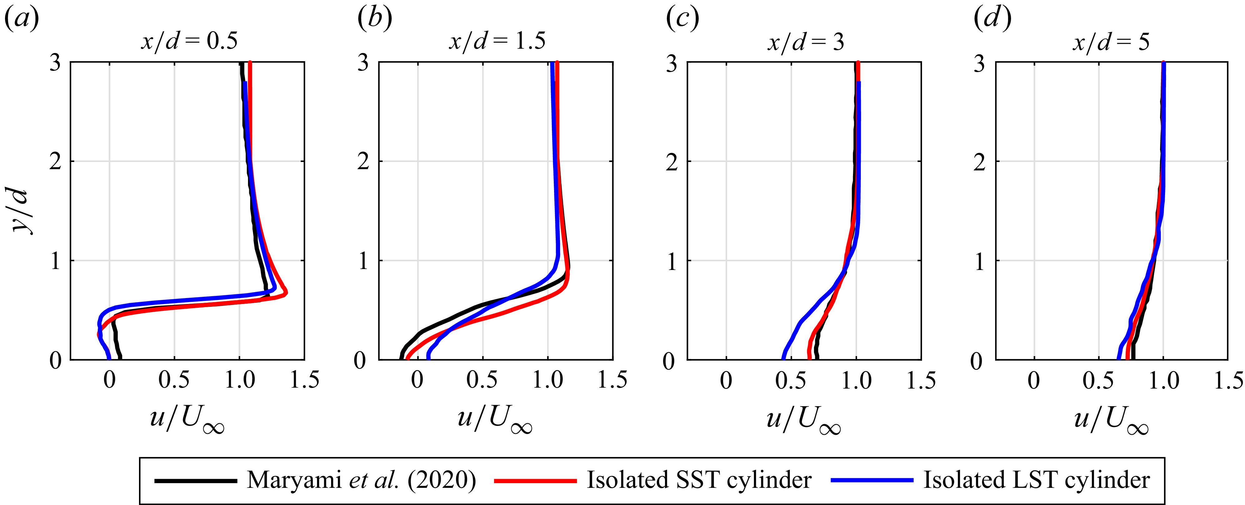
 u/U∞
u/U∞ x/d=0.5,1.5,3,5
 ϕuu
ϕuu ϕvv
ϕvv ϕww
ϕww x/d=5
x/d=5

 θ=60∘
θ=60∘
 u¯rms/U∞
 ω¯zR/U∞
 ωrR/U∞
 r/R=0.7
 r/R=0.99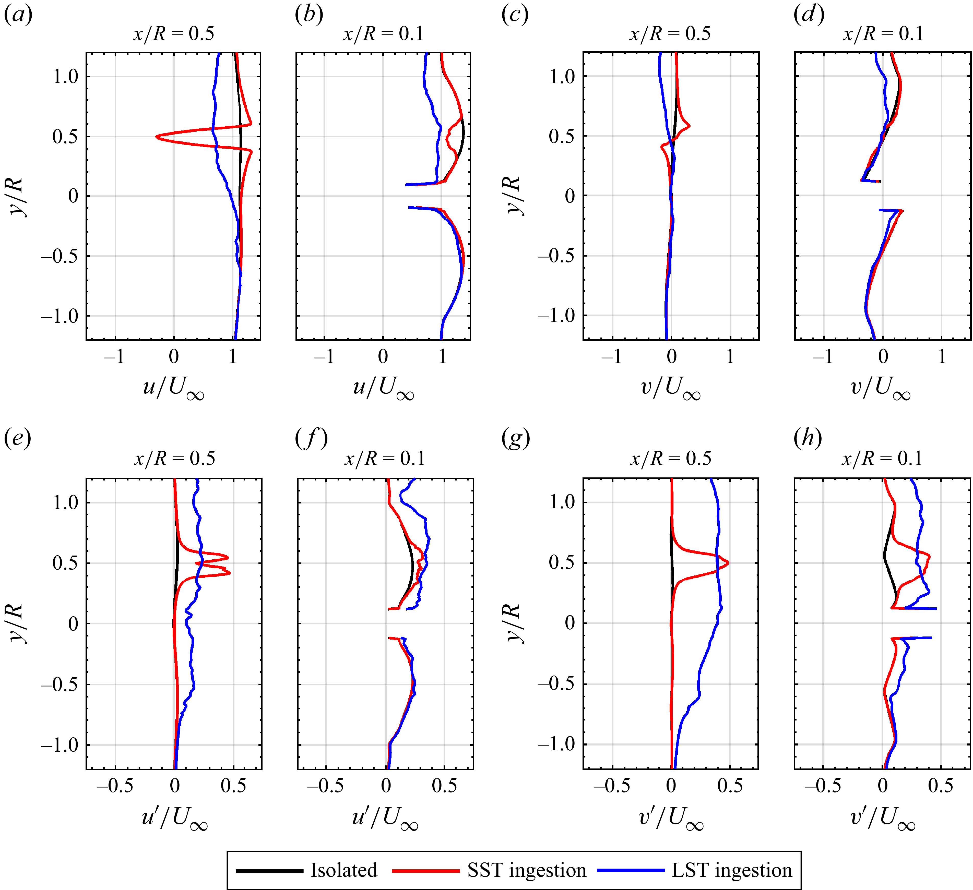
 u/U∞
u/U∞ v/U∞
v/U∞ u′/U∞
u′/U∞ v′/U∞
v′/U∞ 0.5R
0.5R 0.1R
0.1R
 TKE/U∞2
 x/R
x/R y/R=0.5+(dSST,dLST)
 x/R=0.5
 ϕuu(f,x)
 ϕvv(f,x)
 ϕww(f,x)
 x/R
x/R y/R=0.5
 Lu,x(x)
 Lv,x(x)
 Lw,x(x)
 z/R=0,0.5,1
 CT(ψ)
CT(ψ)
 ϕTT(f)
 BPF−nf0
 BPF+nf0
 n=1to3
 prms∗=prms/(ρUtip2)
 θ=90∘
θ=90∘ θ=180∘
 θ
θ
 160Hz
160Hz 10kHz
10kHz SPLm=1
 SPLm=2
 ∂p/∂t
∂p/∂t
 ×
×
 Δ
Δ


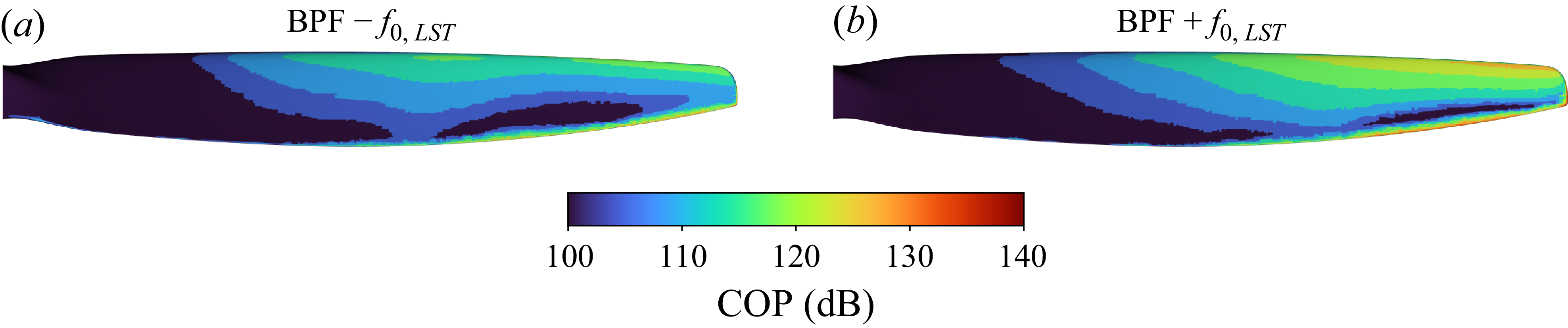
 BPF±f0, LST

 C12(ΔtBPF,r/R)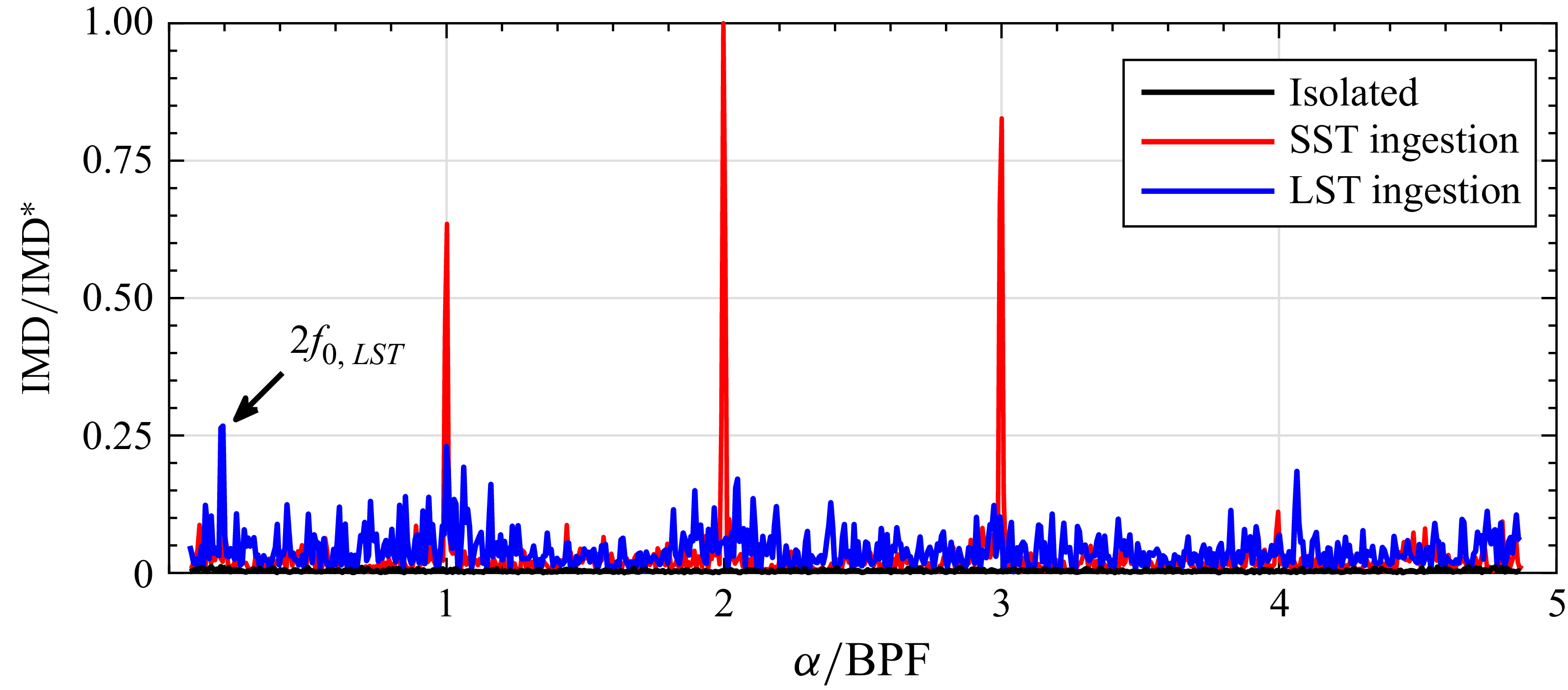

 θ=60∘
θ=60∘
 Cp
Cp z/R=−1.4
 z/R=1.4
 θ=90∘
θ=90∘ θ=180∘
 Open access

