


1. Introduction
The formulation of reliable and robust continuum models for the flow of granular materials has been an important endeavour, owing to the widespread occurrence of granular flows in industrial processes and natural phenomena. While particle cohesion and complex shape are complicating factors in many practical systems, the simpler case of cohesionless granular media composed of roughly isotropic particles is still sufficiently prevalent that modelling them is informative and, to a reasonable extent, generalisable. Early models have focused on two limiting regimes of slow and rapid flow; the flow regime is determined by the Savage number (Savage & Hutter Reference Savage and Hutter1989) or, equivalently, the inertia number  $I$,
$I$,
 \begin{equation} {\mathit{Sa}} \equiv \frac{\rho_p d_p^2 \dot{\gamma}^2}{N} = I^2, \end{equation}
which characterises the contribution of particle inertia to the stress. Here,  $\rho _p$ and $d_p$ are the density and mean diameter of the particles, $\dot {\gamma }$ is the nominal shear rate, and $N$ a stress scale (typically the confining stress). Slow flow corresponds to the limit $Sa \ll 1$, where particle inertia is of no consequence, and rapid flow to $Sa \sim 1$, where particle inertia is dominant. Models for slow flow are based on plasticity theories for soils (Rao & Nott Reference Rao and Nott2008), and models for rapid flows are based on the kinetic theory of dense gases extended to account for inelasticity of particle collisions (Lun et al. Reference Lun, Savage, Jeffrey and Chepurniy1984). The phenomenological $\mu (I)$ model (Jop, Forterre & Pouliquen Reference Jop, Forterre and Pouliquen2006), an extension of a simple plasticity model wherein the friction coefficient is assumed to depend on $I$, has been used to model the intermediate regime between slow and rapid flows. The recent paper of Berzi (Reference Berzi2024) shows that the $\mu (I)$ model can be derived from kinetic theory if spatial correlation of particle velocity fluctuations is accounted for.
In this paper, we restrict attention to the slow-flow regime. Classical plasticity models used for this regime suffer from two major deficiencies. The first is kinematic indeterminacy, meaning that the deformation rate (and therefore the velocity) cannot be uniquely determined if the stress field is specified. This is a consequence of the models being designed to incorporate rate-independence of the stress, an experimentally observed feature of slow flow. The second deficiency is their inability to incorporate shear dilatancy or volume deformation caused by shear deformation; this feature, first observed by Reynolds (Reference Reynolds1885), is peculiar to granular materials and has no analogue in fluids. Dilatancy alters the particle volume fraction field  $\phi$, which in turn affects the stress and therefore the velocity field. Determining the change in $\phi$ due to dilatancy is therefore important in practical problems such as determining the drag on an intruder (Schröter et al. Reference Schröter, Nägle, Radin and Swinney2007).
A few models have successfully resolved the kinematic indeterminacy of classical plasticity models. Mohan, Nott & Rao (Reference Mohan, Nott and Rao1999) and Mohan, Rao & Nott (Reference Mohan, Rao and Nott2002) treated granular media as Cosserat continua, in which stress symmetry is not presumed, thereby requiring that the angular momentum balance be enforced along with the balances of linear momentum and mass. However, asymmetry of the stress has thus far not been experimentally verified. Another class of models introduce a scalar order parameter that is governed by a diffusion equation (Aranson & Tsimring Reference Aranson and Tsimring2002; Bouzid et al. Reference Bouzid, Trulsson, Claudin, Clément and Andreotti2013; Henann & Kamrin Reference Henann and Kamrin2013) in the constitutive relation for the stress. These models are phenomenological, with the order parameter chosen by analogy with other physical systems; moreover, the boundary conditions for the order parameter are speculative. Despite their different physical origins, all the models mentioned above share the common feature of introducing a mesoscopic length scale  $\ell$, whose effect is to allow the material to deform to a distance O( $\ell$) from the point where the yield condition ceases to be satisfied. For this reason, they are called non-local models, though they are not non-local in the formal, mathematical sense (Eringen Reference Eringen1983). Although these models repair kinematic indeterminacy, and their predictions of the velocity profile have been found to be in good agreement with experimental data (Tang et al. Reference Tang, Brzinski, Shearer and Daniels2018; Fazelpour, Tang & Daniels Reference Fazelpour, Tang and Daniels2022; Fazelpour & Daniels Reference Fazelpour and Daniels2023), they all assume the material to be incompressible. As a result, they do not capture shear dilatancy and thereby its effect on the kinematics.
A coupling between the  $\phi$ and $\boldsymbol {u}$ fields was observed in the particle dynamics simulations of Krishnaraj & Nott (Reference Krishnaraj and Nott2016) and Dsouza & Nott (Reference Dsouza and Nott2021), who show that dilatancy in conjunction with gravity drives large-scale secondary flows in cylindrical Couette and split-bottom shear cells. However, very few experimental studies have measured the variation of $\phi$ in three-dimensional (3-D) sheared granular media in the slow-flow regime, as non-invasive imaging of opaque media requires relatively specialised and expensive facilities such as X-ray computed tomography (X-ray CT) and magnetic resonance imaging (MRI). The only study that we are aware of that measured the density field is that of Mueth et al. (Reference Mueth, Debregeas, Karczmar, Eng, Nagel and Jaeger2000), who imaged a cylindrical Couette shear cell using a specialised high-speed MRI facility. While they do find dilation in the shear layer, they report data only very close to the rotating inner cylinder.
Recently, Dsouza & Nott (Reference Dsouza and Nott2020) proposed a model that addresses both the shortcomings of classical plasticity, namely kinematic indeterminacy and absence of dilatancy, by a systematic non-local extension of the critical state plasticity theory. The model poses the flow rule, and the relation between volume fraction and the critical state pressure in a non-local sense without introducing additional variables or equations. Its predictions for plane shear flow were found to be in good agreement with 3-D discrete particle simulations. However, the model predictions have thus far not been validated by experiments.
In this paper, we provide the first experimental measurement of the coupling between the volume fraction and velocity fields in the slow-flow regime, and thereby a verification of the model of Dsouza & Nott (Reference Dsouza and Nott2020), by simultaneously measuring the area fraction and velocity fields in a two-dimensional (2-D) cylindrical Couette shear cell. By imaging a horizontal layer of circular disks sheared between two concentric cylinders, as developed by Tang et al. (Reference Tang, Brzinski, Shearer and Daniels2018), Fazelpour et al. (Reference Fazelpour, Tang and Daniels2022) and Fazelpour & Daniels (Reference Fazelpour and Daniels2023), we measure directly the variation of the azimuthal velocity  $u_\theta$ and $\phi$ with radial distance $r$. While measurements in a 2-D monolayer are not expected to correspond quantitatively with those in three dimensions, it has been shown in several studies that the qualitative features of the kinematics and even the statistics of particle velocity (Ananda, Moka & Nott Reference Ananda, Moka and Nott2008) in two and three dimensions are very similar. By determining the steady-state profiles $u_\theta (r)$ and $\phi (r)$ for different initial $\phi$ profiles (but having the same spatial average), we demonstrate the coupling between the two fields. We compare our experimental data with the predictions of the non-local model of Dsouza & Nott (Reference Dsouza and Nott2020) and find good agreement.
2. Experimental method
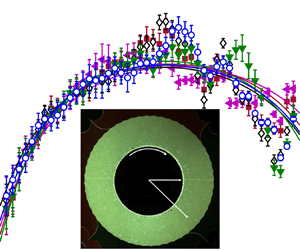
Our experiments are conducted in the 2-D cylindrical Couette rheometer shown in figure 1 described by Fazelpour & Daniels (Reference Fazelpour and Daniels2023). The granular material is confined between coaxial inner and outer cylinders of radii  $r_{i}=16$ cm and $r_o=27$ cm, respectively. The inner cylinder has semi-circular cavities of diameter $d_p$ so that disks settle into them and are carried by the cylinder; this generates sufficient traction to shear the assembly. The inner cylinder is rotated by a motor at a constant angular speed $\varOmega$ such that its azimuthal velocity of $u_{w} \equiv r_i \varOmega = 1.1\ {\rm cm}\ {\rm s}^{-1}$. Each experiment was conducted using an outer cylinder with a specified pattern of roughness (figure 1): two with cavities, two with convex bumps (protrusions) and one made of compliant leaf springs. The dimensions of the roughness features of all the outer cylinders are given in the caption of figure 1.
Top view of 2-D cylindrical Couette device. The inner cylinder of radius  $r_{i}=16$ cm is rotated at constant angular speed $\varOmega$ and the outer cylinder of radius $r_{o}=27$ cm is stationary. The inner cylinder is machined to have semi-circular cavities of diameter $d_p$. The outer cylinder is changeable, and five different roughness designs were used: semi-circular bumps of diameter $d_p$, hereafter called small bumps (SB); bumps of diameter $8 d_p$ and chord length $5.4 d_p$, hereafter called large bumps (LB); semi-circular cavities of diameter $d_p$, hereafter called small cavities (SC); cavities of diameter $8 d_p$ and chord length $5.4 d_p$, hereafter called large cavities (LC); constructed with leaf springs (LS) (see Fazelpour & Daniels Reference Fazelpour and Daniels2023) with the same roughness dimensions as the LB cylinder.

The granular material is composed of polyurethane disks (Vishay Precision Group, PhotoStress material PSM-4) of Young's modulus  $E=4$ MPa and density ${\rho =1.06\ {\rm g}\ {\rm m}^{-3}}$ (Fazelpour & Daniels Reference Fazelpour and Daniels2023). The disks are bidisperse in size, with equal numbers of disks of diameter $0.9d_p$ and $1.1d_p$, where the mean diameter $d_p = 1$ cm. The disks are of thickness 6.35 mm and rest on a flat acrylic base while being sheared between the cylinders. They are placed by hand randomly and distributed as uniformly as possible within the Couette gap. For the 2-D monolayer of disks, the dimensionless density is characterised by the area fraction; hereafter, we use $\phi$ to represent the area fraction of the disks. The roughness of a boundary typically determines the shear rate and velocity slip adjacent to it (Ananda et al. Reference Ananda, Moka and Nott2008; Dsouza & Nott Reference Dsouza and Nott2020). While they are small near the outer cylinder, due to the roughly exponentially decay of $u_{\theta }$ with distance from the inner cylinder, there is a measurable difference in their values for the different outer cylinders. The boundary roughness also plays a role in another way: the initial volume fraction profiles $\phi (r)$ are not identical for the different boundaries. We shall see below that these two effects yield measurably different steady-state profiles of $u_{\theta }$ and $\phi (r)$ in the shear layer near the inner cylinder.
Because the net area available for the disks varies slightly for the different outer cylinders, the number of particles is adjusted to maintain an average area fraction of  $\bar {\phi } = 0.76$. For the outer cylinder composed of LS, the area fraction cannot be held precisely constant due to their compliance; the number of disks used is equal to that for the outer cylinder with LB, which have the same shape.
We track the motion of all particles by imaging the Couette cell by a video camera mounted above the apparatus. The movies are taken at  $30\ {\rm frames}\ {\rm s}^{-1}$ for a duration of 10 min (7 revolutions of the inner cylinder). Each frame in a movie is processed to identify the circular disks and determine their centres $\boldsymbol {x}_i$. The velocities of the disks are computed from their displacement between two successive frames, $\boldsymbol {u}_i = \Delta \boldsymbol {x}_i/\Delta t$. As the flow is axisymmetric and steady, continuum estimates of $u_\theta$ and $\phi$ at radial position $r$ are determined by averaging the particle velocities and their areas within an annular bin of width $\Delta r = 1 d_p$ (centred at $r$) and azimuthal span $0 \leqslant \theta \leqslant {\rm \pi}/2$, and further averaging over a time interval of 200 s (6000 frames). The profiles of $u_\theta$ and $\phi$ are obtained by moving the annular bin by small radial increments to generate data at 48 radial positions. We note that such fine spatial resolution is achieved because we average over large intervals of time and $\theta$, which may not be possible when the flow is unsteady or not fully developed.
The stress field  $\boldsymbol {\sigma }(r)$ was measured for the same set-up and all the outer cylinders by Fazelpour & Daniels (Reference Fazelpour and Daniels2023). As discussed below, we use their measurements of the pressure to determine one of the parameters in the continuum model.
3. The non-local model of Dsouza & Nott
The model of Dsouza & Nott (Reference Dsouza and Nott2020) is based on the idea that the deformation rate  $\boldsymbol{\mathsf{D}}$ at a point depends on the stress $\boldsymbol {\sigma }$ not just at that point, but in a mesoscopic volume surrounding it, as a result of the stress and strain rate being correlated over a mesoscale (such as through force chains). Mathematically, this idea translates to a non-local flow rule (the relation between the strain rate and the stress) and similarly between the volume fraction and the critical state pressure. A mesoscopic length $\ell$, a material parameter, characterises the extent of non-locality. The constitutive relation for $\boldsymbol {\sigma }$ resulting from these arguments is
 $$\begin{gather} \boldsymbol{\sigma} ={-}p \boldsymbol{\delta} + \frac{2\mu}{\dot{\gamma}}(p_c \boldsymbol{\mathsf{D}}'-\ell^2 \varPi \nabla^2 \boldsymbol{\mathsf{D}}'), \end{gather}$$
 $$\begin{gather}p = p_c \left(1- \frac{\mu _b}{\dot{\gamma}} \boldsymbol{\nabla} \boldsymbol{\cdot} \boldsymbol{u}\right) + \ell^2 \varPi \frac{\mu _b}{\dot{\gamma}}\nabla ^2 \boldsymbol{\nabla} \boldsymbol{\cdot} \boldsymbol{u}, \end{gather}$$
 $$\begin{gather}p_c =\varPi - \ell^2 \frac{{\rm d}\varPi}{{\rm d}\phi}\nabla ^2 \phi, \end{gather}$$
where  $\boldsymbol{\mathsf{D}}' \equiv \boldsymbol{\mathsf{D}} - \frac {1}{3}\boldsymbol {\nabla } \boldsymbol {\cdot } \boldsymbol {u} \, \boldsymbol {\delta }$ is the deviatoric part of $\boldsymbol{\mathsf{D}}$ and $\dot {\gamma } \equiv (2\boldsymbol{\mathsf{D}}' : \boldsymbol{\mathsf{D}}')^{1/2}$ is its scalar invariant, $p$ is the pressure and $p_c$ the pressure at the critical state. The terms multiplied by $\ell ^2$ are the non-local contributions to the constitutive relation. The material properties are the friction coefficients $\mu$ and $\mu _b$ for shear and volume deformation, respectively, the mesoscopic length $\ell$ and the local form of the critical state pressure $\varPi (\phi )$.
We now apply the non-local model (3.1) to shear in a 2-D cylindrical Couette cell, for which the deviatoric deformation rate tensor is  $\boldsymbol{\mathsf{D}}' \equiv \boldsymbol{\mathsf{D}} - \frac {1}{2}\boldsymbol {\nabla } \boldsymbol {\cdot } \boldsymbol {u} \, \boldsymbol {\delta }$ and $\phi$ represents the area fraction. The governing equations are the balances of mass, and the $r$ and $\theta$ components of momentum. For steady axisymmetric flow, the mass balance is trivially satisfied, and the $r$ and $\theta$ momentum balances reduce to
 \begin{equation} \partial \sigma_{rr}/\partial r = 0, \quad (1/r^2) \partial/\partial r (r^2 \sigma_{r \theta}) +\mu_{base}\, \phi \rho_p g = 0. \end{equation}
The second term in (3.2b) is the frictional resistance offered by the base. On substituting the constitutive relation for  $\boldsymbol {\sigma }$ (3.1), the momentum balances (3.2) take the form
 $$\begin{gather} \frac{{\rm d}}{{\rm d}r} \left[ \varPi - l^2\, \frac{{\rm d}\varPi}{{\rm d} \phi} \left( \frac{{\rm d}^2 \phi}{{\rm d}r^2} + \frac{1}{r} \frac{{\rm d} \phi}{{\rm d} r} \right) \right] = 0, \end{gather}$$
 $$\begin{gather} \frac{1}{r^2} \frac{{\rm d}}{{\rm d} r} \left[ r^2 \frac{\mu p_c}{\dot{\gamma}} \left(\frac{{\rm d}u_{\theta}}{{\rm d}r} - \frac{u_{\theta}}{r} \right)- r^2 \ell^2 \, \frac{\mu \varPi}{\dot{\gamma}} \left(\frac{{\rm d}^3 u_{\theta}}{{\rm d}r^3} + \frac{1}{r^2} \frac{{\rm d}u_{\theta}}{{\rm d}r} - \frac{u_{\theta}}{r^3} \right) \right] - \mu_{base}\, \phi \rho_pg = 0, \end{gather}$$
where  $\dot {\gamma } = |{\rm d}u_{\theta }/{\rm d}r - u_{\theta }/r|$.
To close (3.3), four boundary conditions for  $u_{\theta }$ and three for $\phi$ are required. Unlike fluids, granular media usually slip at rigid boundaries (Natarajan, Hunt & Taylor Reference Natarajan, Hunt and Taylor1995; Ananda et al. Reference Ananda, Moka and Nott2008), and accounting for slip is often important. A boundary condition that accommodates slip was proposed by Mohan et al. (Reference Mohan, Rao and Nott2002) for their Cosserat continuum model in which the slip velocity is $K d_p \boldsymbol {n} \times \boldsymbol {\omega }$, where $K$ is the slip coefficient and $\boldsymbol {\omega }$ is the rate of material spin at the boundary of unit normal $\boldsymbol {n}$. For a classical continuum, $\boldsymbol {\omega }$ is equal to half the vorticity $\boldsymbol {w}$; the two fields can differ in Cosserat continua and the difference is proportional to the asymmetry of the Cauchy stress (Dahler Reference Dahler1959; Lun Reference Lun1991; Mohan et al. Reference Mohan, Rao and Nott2002). As there is little experimental evidence for asymmetry of the Cauchy stress in granular media, we proceed with the assumption that the granular medium is a classical continuum, and hence $\boldsymbol {\omega } = \boldsymbol {w}$. Using this condition and the wall friction boundary condition (Rao & Nott Reference Rao and Nott2008), we have
 \begin{equation} u_{\theta} - u_{w} = K d_p \left( \frac{{\rm d}u_{\theta}}{{\rm d} r} + \frac{u_{\theta}}{r} \right), \quad \frac{-\sigma_{r \theta}}{\sigma_{rr}} = \mu_w \quad \mbox{at}\ r = r_i, \end{equation}
where  $\mu _w$ is the friction coefficient between the inner wall and the granular material. At steady state, the shear stress $\sigma _{r\theta }$ decreases with $r$ while the normal stress $\sigma _{rr}$ is constant, whence $|\sigma _{r\theta }/\sigma _{rr}|$ decreases with $r$. For large enough Couette gap, non-local effects cannot transmit shear to the outer wall, whence the shear rate there must vanish (Mohan et al. Reference Mohan, Rao and Nott2002; Dsouza & Nott Reference Dsouza and Nott2020). Together with the slip condition (3.4a), we get the boundary conditions
 \begin{equation} u_{\theta}=0, \quad \frac{{\mathrm d} u_{\theta}}{{\mathrm d} r} = 0 \quad \mbox{at}\ r = r_o. \end{equation}
The value of the slip coefficient  $K$ in (3.4a) will depend on the nature of the boundary; in studies where the boundaries are topographically roughened, such as by gluing coarse sandpaper to the wall, the slip velocity has been found to be small, implying $K = 0$. For a given wall, $K$ must be determined by fitting with experimental data for the velocity. Jing et al. (Reference Jing, Kwok, Leung and Sobral2016) correlated the slip velocity in an inclined chute with the roughness parameters of the base using discrete element method simulations; generalising such a study to determine $K$ as a function of the wall roughness features and $\phi$ would be a useful exercise.
For the area fraction  $\phi$, one obvious condition is that the mean solids fraction $\bar {\phi }$, or alternatively the normal stress at one of the boundaries, must be specified. Apart from that, we do not have other well-established boundary conditions for $\phi$ at the walls. We follow Dsouza & Nott (Reference Dsouza and Nott2020) and assume that $\phi$ at the two boundaries are known; we discuss this choice in § 5. As a result, we have the following conditions for $\phi$:
 \begin{equation} \int_{r_i}^{r_o} \phi 2 {\rm \pi}r \,{\mathrm d} r = \bar{\phi} \, {\rm \pi}(r^2_o - r^2_i), \quad \phi (r_i) = \phi_i, \quad \phi (r_o) = \phi_o. \end{equation}
 Equations (3.3)–(3.6) constitute a well-posed boundary value problem. Note that the momentum balances (3.3a) and (3.3b) are uncoupled; solution of the former yields the area fraction profile  $\phi (r)$ and the latter then yields the velocity profile $u_\theta (r)$. The equations are solved by the finite difference method using second-order discretisation. The resulting nonlinear algebraic equations for $u_\theta$ and $\phi$ at the $N$ discretised values of $r$ are solved using the nonlinear equation solver fsolve in MATLAB. The results reported in § 4 are for $N = 100$; the solutions remain unchanged (to within a relative tolerance of $10^{-3}$) for larger $N$.
$N$.
4. Results and discussion
For numerical solution of the governing equations (3.3)–(3.6), the values of parameters that characterise the granular material and the boundaries are needed. To solve (3.4a), we need the form of the function  $\varPi (\phi )$ in the expression for the critical state pressure (3.1c); as done by Dsouza & Nott (Reference Dsouza and Nott2020), we assume the form proposed by Nott & Jackson (Reference Nott and Jackson1992),
 \begin{equation} \varPi(\phi) = \left\{ \begin{array}{@{}ll@{}} \alpha \dfrac{(\phi - \phi_{min})^{n_1}}{(\phi_{max} - \phi)^{n_2}}, & \phi \geqslant \phi_{min},\\ 0, & \phi < \phi_{min}, \end{array} \right. \end{equation}
where  $\phi _{min} = 0.65$ and $\phi _{max} = 0.82$ are the area fractions for loose and dense random packing, respectively. For a 2-D layer of particles, we expect the exponents $n_1$ and $n_2$ to differ from the values used for 3-D assemblies by Nott & Jackson (Reference Nott and Jackson1992) and Dsouza & Nott (Reference Dsouza and Nott2020). We determine them by minimising the error between the model predictions and the experimental data for $\phi (r)$ for the outer cylinder with LB (see figure 1). The constant $\alpha$ is estimated from the measurement by Fazelpour & Daniels (Reference Fazelpour and Daniels2023) of the pressure $p \approx 10^3$ Pa for $\bar {\phi } = 0.76$, which yields the value $\alpha = 30$ Pa. To solve (3.4b), we need values for the three friction coefficients, the slip coefficient $K$ and the mesoscopic length $\ell$. We retain the value $\ell = 10$ used in all our previous studies (Mohan et al. Reference Mohan, Rao and Nott2002; Ananda et al. Reference Ananda, Moka and Nott2008; Dsouza & Nott Reference Dsouza and Nott2020). By integrating (3.3b) once from $r_i$ to $r$ and using the boundary condition (3.4b), we see that the friction coefficients occur only as the ratios $\mu _w/\mu$ and $\mu _{base}/\mu$. These ratios and $K$ are determined by minimising the error between the model predictions and the experimental data for $u_\theta (r)$ for the LB outer cylinder. Details of parameter estimation by minimising the error are given in the Appendix. The best-fit set of model parameters are $n_1 = 2$, $n_2 = 1$, $\mu _w/\mu = 1$, $\mu _{base}/\mu = 3.76$ and $K = 0.63$. The parameters are now fixed at these values and used for comparison against all the other experimental data sets.
The experimental data for the LB outer cylinder are shown in figure 2, along with the model predictions using the best-fit parameter values. A notable feature of the experimental data is that the initial area fraction profile (i.e. before shearing has commenced) has significant spatial fluctuations about the mean  $\bar {\phi } = 0.76$. They arise because the disks are placed in the Couette gap by hand, whence some non-uniformity is unavoidable. Moreover, $\phi$ is lower near the inner and outer cylinders due to packing constraints near rigid boundaries. As the material is sheared, we observe the development of pronounced dilation (reduction of $\phi$) in the shear layer near the inner cylinder; concurrently, the fluctuations in $\phi$ become smoother and ultimately vanish at steady state. Conservation of mass leads to some compaction at larger radial positions, but the fluctuations in $\phi$ in the outer half of the Couette gap remain even after prolonged shear. This is because the velocity and shear rate decay roughly exponentially with distance from the inner cylinder (figure 2(b) and inset of figure 4b), thereby causing little rearrangement of the packing away from the inner cylinder.
Experimental data and model predictions for the outer cylinder with LB, see figure 1. ( $a$) Data for the area fraction $\phi (r)$ before shear is commenced and at steady state compared with the model prediction using the best-fit parameters values $n_1 = 2$ and $n_2 = 1$ and $\alpha = 30$ Pa. ( $b$) Data for the velocity $u_\theta (r)$ at steady state compared with the model predictions using the best-fit parameters values $\mu _w/\mu = 0.99$, $\mu _{base}/\mu = 3.76$ and $K = 0.63$. The best-fit parameters are obtained by minimising the error between the model predictions and the data (see the Appendix).

A brief discussion on how dilatancy arises in the model is pertinent. At the steady state, which in the present problem is the critical state, the momentum balance in the  $r$ direction (3.3a) requires the critical state pressure $p_c$ to be constant across the Couette gap. The non-local relation between $p_c$ and $\phi$ results in the spatial variation in $\phi$ across the Couette gap such that $\phi$ is lower in the shear layer, i.e. dilatancy. In the absence of the non-local contribution to $p_c$, namely the second term on the right-hand side of (3.1c), $\phi$ is constant and there is no dilatancy. The physical mechanism for the evolution of $\phi$ from the initial state, by depletion of particles from the shear layer and accumulation further away, becomes clear when we consider the unsteady development of the flow fields in § 4.1.
As described in § 2, experiments were conducted with outer cylinders of different roughness patterns. Figure 3 compares the area fraction and velocity profiles and the corresponding model predictions (solid lines) for all the cylinders. We observe that the profiles of  $\phi$ and $u_\theta$ in all the cases are quite similar: there is substantial dilation near the inner cylinder (figure 3a), where the velocity gradient is high (figure 3b), and the velocity profiles decay roughly exponentially.
Data for the five different outer cylinders (see figure 1) and the corresponding model predictions. ( $a$) Area fraction profiles, with the mean area fraction being $\bar {\phi } = 0.76$ in all the cases. ( $b$) Azimuthal velocity profiles scaled by the velocity of the inner cylinder. The solid lines are the model predictions and the symbols with error bars are experimental data.

Nevertheless, there are slight variations between the  $\phi (r)$ and $u_\theta (r)$ profiles for outer cylinders of different roughness, possibly due to the differences in the initial area fraction profile. Since the shear rate is very small ( ${\sim }10^{-5}\ {\rm s}^{-1}$) in the outer portion of the Couette gap, it is likely that the small differences in the mean area fraction within the shear layer remain even at steady state. Serendipitously, these differences turn out to be useful in demonstrating a key aspect of the model, namely the coupling between the packing fraction and velocity fields. Figure 4 compares the steady-state profiles for the outer cylinder with LS and LB. Despite the error bars, a small but systematic difference in the steady-state area fraction profiles is evident. For the cylinder with LS, $\phi$ is lower near the inner cylinder and higher at larger $r$. Figure 4( $b$) shows that this results in a measurable difference in the $u_\theta$ profiles, which are in agreement with the model predictions. To further establish the coupling, we have shown in figure 4( $b$) the velocity profile obtained by assuming the area fraction to be constant, i.e. $\phi (r) = \bar {\phi }$; it is clear the velocity profile differs substantially from those corresponding to the dilated steady states. Thus, the data show clearly the inter-dependence of the packing fraction and velocity profiles, which was demonstrated earlier in Dsouza & Nott (Reference Dsouza and Nott2020) using particle simulations.
Experimental data (symbols) for ( $a$) area fraction and ( $b$) azimuthal velocity $u_\theta$ for the outer cylinders with LS and LB compared with the model predictions (solid lines). The mean area fraction in both the cases is $\bar {\phi } = 0.76$. The blue dashed line in panel ( $b$) is the model prediction obtained by assuming the area fraction to be constant, i.e. $\phi (r) = \bar {\phi }$. The inset in panel ( $b$) shows the velocity on a logarithmic scale; data for $y > 0.5$ are not shown, as $u_\theta /u_w$ approaches the measurement resolution ( ${\approx }10^{-3}$).

4.1. Unsteady evolution of the packing fraction and velocity fields
Thus far, we have shown the predictions of the model for the steady state and compared them with the experimental data. As already noted, for the steady state, momentum balances in the  $r$ and $\theta$ directions are uncoupled, allowing the determination of $\phi$ first and then $u_\theta$. We now consider the unsteady evolution of the flow fields from the initial un-sheared state, where the packing fraction and velocity fields evolve together, and the mechanism in the model that captures dilatancy becomes much clearer.
We expect the presence of a radial velocity  $u_r$ and therefore a non-zero bulk deformation rate $\boldsymbol {\nabla } \boldsymbol {\cdot } \boldsymbol {u} = \partial u_r/\partial r + u_r/r$. Discarding the inertial terms in the unsteady momentum balances, as our interest is in the slow-flow regime, the equations of motion for axisymmetric unsteady flow are
 \begin{align} &\frac{\partial \phi}{\partial t} + \frac{1}{r} \frac{\partial}{\partial r} (r \phi u_r)=0, \end{align}
 \begin{align} &- \frac{\partial p}{\partial r} + \left(\frac{2}{r} + \frac{\partial}{\partial r} \right) \left[ \frac{\mu p_c}{\dot{\gamma}} \left(\frac{\partial u_r}{\partial r} - \frac{u_r}{r} \right) - \ell^2 \, \frac{\mu \varPi}{\dot{\gamma}} \left(\frac{\partial^3 u_r}{\partial r^3} + \frac{1}{r^2} \frac{\partial u_r}{\partial r} - \frac{u_r}{r^3} \right) \right] \nonumber\\ &\quad- \mu_{base}\, \phi \rho_pg \frac{u_r}{(u_r^2 + u_\theta^2)^{1/2}} = 0, \end{align}
 \begin{align} &\frac{1}{r^2} \frac{\partial}{\partial r} \left[ r^2 \frac{\mu p_c}{\dot{\gamma}} \left(\frac{\partial u_{\theta}}{\partial r} - \frac{u_{\theta}}{r} \right) - r^2 \ell^2 \, \frac{\mu \varPi}{\dot{\gamma}} \left(\frac{\partial^3 u_{\theta}}{\partial r^3} + \frac{1}{r^2} \frac{\partial u_{\theta}}{\partial r} - \frac{u_{\theta}}{r^3} \right) \right] \nonumber\\ &\quad - \mu_{base}\, \phi \rho_pg \frac{u_\theta}{(u_r^2 + u_\theta^2)^{1/2}} = 0, \end{align}
with the pressure  $p$ given by (3.1b) and $\dot {\gamma } = [ (\partial u_{\theta }/\partial r - u_{\theta }/r)^2 + (\partial u_r/\partial r - u_r/r)^2 ]^{1/2}$.
Since the momentum balances are quasistatic, solution of (4.2) requires an initial condition only for  $\phi$, for which we use the initial distribution $\phi _0(r)$,
 \begin{equation} \phi(0,r) = \phi_0(r). \end{equation}
Additionally, we require four boundary conditions for  $u_r$. Two obvious conditions are no penetration at the walls. For the two additional conditions, we propose that the ratio of dilation rate normal to a wall to the tangential shear rate is proportional to the departure from the critical state,
 \begin{equation} (\boldsymbol{\nabla} \boldsymbol{\cdot} \boldsymbol{u})_n /\dot{\gamma}_t = \beta (\phi - \phi_c), \end{equation}
where  $(\boldsymbol {\nabla } \boldsymbol {\cdot } \boldsymbol {u})_n \equiv \boldsymbol {n} \boldsymbol {\cdot } \boldsymbol{\mathsf{D}} \boldsymbol {\cdot } \boldsymbol {n}$ and $\dot {\gamma }_t \equiv |\boldsymbol {n} \boldsymbol {\cdot } \boldsymbol{\mathsf{D}}' \boldsymbol {\cdot } \boldsymbol {t}|$, $\boldsymbol {n}$ and $\boldsymbol {t}$ are the unit normal and unit tangent in the flow direction, $\phi _c$ is the packing fraction at the critical state (which here is the steady state), and $\beta$ is a constant. As $\dot {\gamma }_t$ vanishes at the outer cylinder (see (3.5)), (4.4) implies that the dilation rate also vanishes. The boundary conditions for $u_r$ then are
 $$\begin{gather} u_r = 0, \quad \frac{2}{|\partial u_{\theta}/\partial r - u_{\theta}/r|} \frac{\partial u_r}{\partial r} = \beta (\phi - \phi_i) \quad \mbox{at}\ r = r_i, \end{gather}$$
 $$\begin{gather} u_r = 0, \quad \frac{\partial u_r}{\partial r} = 0 \quad \mbox{at}\ r = r_o. \end{gather}$$
For the reasons mentioned at the end of this section, we do not attempt to determine  $\beta$ by fitting with experimental data; however, we find that $\beta = 1$ gives a reasonable match with experiments for the time scale to approach steady state.
Equations (4.2) with initial condition (4.3) and boundary conditions (3.4)–(3.6) and (4.5) form a well-posed problem. They are solved numerically in the same manner as in § 3. As an illustrative example, we determine the unsteady solution starting from an initial state corresponding to the data for the outer cylinder with large bumps, shown in figure 2( $a$). We take $\phi _0(r)$ to be a smoothed fit of the data, shown in the inset of figure 5( $a$). The model prediction of the unsteady evolution of the $\phi$ and velocity fields are shown in figure 5. The mechanism for dilatancy now becomes clear – we see that a radial velocity $u_r$ develops in the transient state (figure 5 $b$), which convects particles away from the region of high shear rate, thereby reducing $\phi$ near the inner cylinder (figure 5 $a$). The radial velocity decays with time, and at steady (critical) state, $\phi (r)$ is determined by the constraint of constant pressure (3.2a). Thus, the non-local contribution to $p_c$ in (3.1c) is essential for the non-uniform distribution of $\phi$. As dilatancy proceeds, we see in figure 5( $c$) that the sharpness in the decay of the primary velocity $u_\theta$ increases. Thus, the unsteady evolution illustrates the physical mechanism in the model that leads to dilatancy via convection of particles away from the shear layer, and how that couples with the velocity field.
Unsteady evolution of the packing fraction and velocity profiles with dimensionless time  $\hat {t} \equiv t u_w/(r_o - r_i)$. The flow is taken to be axisymmetric. ( $a$) Evolution of the $\phi$ profile. The inset shows the initial condition $\phi _0(r)$, which is a smoothed fit of initial state in the experiment for the LB outer cylinder (see figure 2 $a$). ( $b$) Evolution of the radial velocity $u_r$; note that $u_r$ is everywhere positive, largest near (but not at) the inner cylinder and decays to zero at large $\hat {t}$. ( $c$) Evolution of the azimuthal velocity $u_\theta$; the decay with distance from the inner cylinder becomes more rapid with time, due to depletion of particles near the inner cylinder.

We are unable to make a comparison of the transient profiles in figure 5 with experimental data, as the unsteady data are noisy. As explained in § 2, obtaining smooth profiles with reasonable spatial resolution requires averaging over a long period of time, which is not possible in the transient state.
5. Discussion and conclusion
We have presented experimental data for the profiles of the area fraction  $\phi$ and the azimuthal velocity $u_\theta$ for the shear of disks in a 2-D cylindrical Couette cell. At steady state, we find the velocity to decay roughly exponentially with radial distance from the rotating inner cylinder, in agreement with the findings of previous studies (Howell, Behringer & Veje Reference Howell, Behringer and Veje1999; Losert et al. Reference Losert, Bocquet, Lubensky and Gollub2000; Mueth et al. Reference Mueth, Debregeas, Karczmar, Eng, Nagel and Jaeger2000). Shear causes pronounced dilation, or reduction in $\phi$, in the shear layer, and mass conservation results in compaction at larger radial positions. The experimental data are in good agreement with the predictions of the non-local model of Dsouza & Nott (Reference Dsouza and Nott2020). To our knowledge, this is the first systematic experimental measurement of dilatancy at constant volume and the coupling between packing fraction and velocity fields for granular materials in the slow-flow regime.
As elaborated in § 1, classical plasticity models, which have been traditionally used for slow granular flow, suffer from two major inadequacies: kinematic indeterminacy and inability to capture shear dilatancy. The former is associated with the mathematical ill-posedness of the models (Barker et al. Reference Barker, Schaeer, Bohorquez and Gray2015). While a few models have been proposed to repair kinematic indeterminacy, they treat the medium as incompressible. The non-local model of Dsouza & Nott (Reference Dsouza and Nott2020) treats the medium as compressible and builds in dilatancy. The experimental validation of the model is therefore a useful advance, and highlights the importance of incorporating dilatancy in models for slow granular flow. It is pertinent to note that Andrade et al. (Reference Andrade, Chen, Le, Avila and Matthew Evans2012) proposed a model for the rate-dependent regime, where they introduced a phenomenological dilatancy function  $\beta \equiv \boldsymbol {\nabla } \boldsymbol {\cdot } \boldsymbol {u}/\dot {\gamma }$ which decays with increasing shear strain; to capture the effect of dilatancy, they solved the time-dependent problem. In the model of Dsouza & Nott (Reference Dsouza and Nott2020), dilatancy arises naturally from the momentum balances; no additional function needs to be introduced and the steady-state solution can be obtained directly.
Though the model of Dsouza & Nott (Reference Dsouza and Nott2020) is formulated for the (non-inertial) slow-flow regime, it can be extend to include the effects of particle inertia by using the ansatz of the  $\mu (I)$ model (GDR MiDi 2004; Jop et al. Reference Jop, Forterre and Pouliquen2006), i.e. by considering $\mu$ to be a function of the inertia number $I$. We hope that our study will spur other investigations to probe the effect of inertia on dilatancy and its coupling to kinematics. A shortcoming of the model prediction is that we have used the experimentally measured values of $\phi$ at the two cylinders as the boundary conditions for that variable. Ideally, one would like a boundary condition that specifies $\phi$ (or its gradient) as a function of the normal stress and the kinematic state of the material. Deriving such a boundary condition from a first principles approach is an important exercise and requires further investigation.
We were only able to study the effect of small variations in the  $\phi$ profile (keeping its average $\bar {\phi }$ constant) on the velocity profile. While our data do provide evidence of the inter-dependence of the two fields, it would nevertheless be useful to achieve larger variations in $\phi (r)$, such as by altering the roughness of the inner cylinder, in a future investigation. Finally, our study points to the need for precise non-invasive measurement of the volume fraction field in granular flow. Despite X-ray CT and MRI being expensive and not widely available, using them to study a few complex three-dimensional flows would be worthwhile to validate and refine models.
Acknowledgement
We are grateful to M. Louge for suggesting the collaboration between the groups of K.E.D. and P.R.N.
Funding
This work was partially supported by the Anusandhan National Research Foundation under grant CRG/2021/005775, the International Fine Particle Research Institute and the National Science Foundation under award nos NSF DMR-1206808 and DMR-2104986. K.E.D. acknowledges support from the Fulbright-Nehru fellowship program.
Declaration of interests
The authors report no conflict of interest.
Appendix. Estimation of the model parameters
We determine the values of parameters from the experimental data for the outer cylinder with LB (see figure 1). The 2-norm of the errors in the predicted area fraction and velocity are
 \begin{equation} E_\phi^2 \equiv \frac{1}{N}\sum_{n=1}^{N} (\Delta\phi(r_n))^2, \quad E_u^2 \equiv \frac{1}{N}\sum_{n=1}^{N} (\Delta u_{\theta}(r_n))^2 ,\end{equation}
where  $\Delta \phi (r_n)$ and $\Delta u_{\theta }(r_n)$ are the differences between the model prediction and experimental data for $\phi$ and $u_{\theta }$, respectively, at the finite difference nodes $r_n$. The parameters $n_1$ and $n_2$ are determined by minimising $E_\phi$, and the parameters $K$,
$K$,  $\mu _w/\mu$ and $\mu _{base}/\mu$ are estimated by minimising $E_{u}$. Figure 6( $a$) shows that $E_\phi$ is minimum at $n_1 = 2$, $n_2=1$. We only explore integer values of the indices $n_1$ and $n_2$, as data on the dependence of the pressure at critical state with $\phi$ are sparse; we were therefore content with a rough determination of the functional form of $\varPi (\phi )$. Solution of (3.3b) for $u_\theta (r)$ requires $\varPi (\phi )$ and the parameters $K$,
$K$,  $\mu _w/\mu$ and $\mu _{base}/\mu$. The model prediction and thereby $E_{u}$ are computed using the above-determined values of $n_1$ and $n_2=1$, and for a range of the other three parameters. Figures 6( $b$) and 6( $c$) show that $E_{u}$ is minimum for the values $K = 0.63$, $\mu _{base}/\mu = 3.76$ and $\mu _w/\mu = 0.99$. The parameter set thus obtained is used to make predictions for all the other outer cylinder designs described in § 2.
Parameter estimation for the LB outer cylinder. In each panel, the filled circle identifies the parameter values that minimise the error, and the colour bars indicate the magnitude of the error. ( $a$) Contours of constant $E_\phi$ in the $(n_1, n_2)$ plane. The difference is minimum at $n_1 = 2$, $n_2 = 1$. (b,c) Contours of constant $E_u$ in the $(K, \mu _{base}/\mu, \mu _w/\mu )$ space; the two panels show two orthogonal planes passing through the point $K = 0.63$, $\mu _{base}/\mu = 3.76$, $\mu _w/\mu = 0.99$ at which $E_u$ is minimum.


 Open access